Polarization Angle Orthogonal Jumps in Fast Radio Bursts

Abstract

Recently, polarization angle (PA) orthogonal jumps over millisecond timescale were discovered from three bursts of a repeating fast radio burst source FRB 20201124A by the FAST telescope. We investigate the physical implications of this phenomenon. In general, PA jumps can arise from the superposition of two electromagnetic waves, either coherently or incoherently, as the dominance of the two orthogonal modes switches. In the coherent case, PA jumps occur when linear polarization reaches a minimum and circular polarization peaks, with the total polarization degree conserved. However, incoherent superposition can lead to depolarization. The observations seem to be more consistent with incoherent superposition. The amplitudes of the two orthogonal modes are required to be comparable when jumps occur, placing constraints on the intrinsic radiation mechanisms. We provide general constraints on FRB emission and propagation mechanisms based on the data. Physically, it is difficult to produce PA jumps by generating two orthogonal modes within millisecond timescales, and a geometric effect due to sweeping line-of-sight is a more plausible reason. This requires the emission region to be within the magnetosphere of a spinning central engine, likely a magnetar. The two orthogonal modes may be produced by intrinsic radiation mechanisms or Alfvén-O-mode transition. Plasma birefringence is not easy to achieve when the plasma is moving relativistically. Curvature radiation predicts $|E_{\rm X}/E_{\rm O}|\gtrsim 1$, and is difficult to produce jumps; whereas inverse Compton scattering can achieve the transition amplitude ratio $|E_{\rm X}/E_{\rm O}|=1$ to allow jumps to occur under special geometric configurations.

1 Introduction

Fast radio bursts (FRBs) are bright millisecond-duration astronomical transients predominantly originating from cosmological distances (Lorimer et al., 2007; Thornton et al., 2013). The connection between FRBs and magnetar was confirmed with the detection of FRB 20200428 from one Galactic magnetar SGR 1935+2154 (Bochenek et al., 2020; CHIME/FRB Collaboration et al., 2020) implying that at least some FRBs can be produced by magnetars. However, the source origins of FRBs are still subject to debate. Additionally, the high brightness temperatures $\sim 10^{35}$ K require the radiation mechanisms must be coherent, which are also puzzling.

Growing observational results can provide essential clues on the radiation mechanisms and properties of emission regions (Zhang, 2023). One of the dominant feature of repeating FRBs is polarization information. Interestingly, current data from both repeating and non-repeating FRBs show interesting but puzzling features regarding diverse features of polarization angle (PA). Observationally, the PA as a function of time within individual bursts either shows a flat (non-evolution) or a varying behavior. Interesting observational facts can be summarized as follows:

• Flat PA temporal evolution has been detected in most active repeating FRBs (e.g. FRB 20121102A (Gajjar et al., 2018; Michilli et al., 2018), FRB 20180916B (CHIME/FRB Collaboration et al., 2019; Chawla et al., 2020; Nimmo et al., 2021), FRB 20190711A (Day et al., 2020; Kumar et al., 2021), FRB 20190303A and FRB 20190417A (Feng et al., 2022), FRB 20190604A (Fonseca et al., 2020), FRB 20201124A (Xu et al., 2022; Jiang et al., 2022)). In some of these sources, both flat and varying PA evolution have been observed. In most cases for both flat and varying PAs, high linear polarization with $\Pi_{L}\gtrsim 95\%$ is usually detected.

• The phenomena of varying PA include two general cases: PA swings (regular S-shaped or irregular swing) and PA jumps. Various regular and irregular PA swings have been observed in some individual bursts of FRB 20180301A (Luo et al., 2020; Feng et al., 2022) and FRB 20220912A (Zhang et al., 2023).

  For the regular S-shaped PA case, some bursts can be well described by the rotating vector model (RVM) (Radhakrishnan & Rankin, 1990) commonly invoked to study the evolution of pulsar PA. One example is a non-repeating FRB 20221022A detected by the Canadian Hydrogen Intensity Mapping Experiment (CHIME) (Mckinven et al., 2024), suggesting a natural connection between FRBs and magnetospheric emission similar to pulsar radio emission. However, for repeating sources such as FRB 20180301A (Luo et al., 2020), no unified RVM model works for all the bursts, suggesting a dynamically varying magnetosphere in FRB sources.

• Recently, the first polarization angle ninety-degree jump from FRB 20201124A was detected with Five-hundred-meter Aperture Spherical radio Telescope (FAST) (Niu et al., 2024; Jiang et al., 2024). The PA jumps were detected in three bursts with transition timescale of several milliseconds. The jumps occurr when the linear polarization degree becomes minimum and the total polarization degree is not conserved. Both temporal evolution and polarization properties can provide insightful information on intrinsic radiation mechanisms of FRBs. PA jumps have been widely observed (Manchester et al., 1975; Backer et al., 1976; Stinebring et al., 1984) in radio pulsars, and different orthogonal modes transition processes have been investigated within the framework of radio pulsars (McKinnon, 2024). The detection of such jumps suggests that FRB emission may share a similar radiation or propagation mechanism. Superposition of two orthogonal modes has been proposed to explain the PA jumps in both pulsar radio emission and FRBs (Stinebring et al., 1984; Niu et al., 2024).

In general, the temporal jump of PA within milliseconds can be attributed to either a physical change of the plasma condition within a millisecond timescale or a geometric effect due to the line of sight (LOS) sweeping different emission regions. For the latter possibility, emissions from two orthogonal modes should be directed in different directions. This can be achieved via either intrinsic mechanisms or geometric effects. In this paper, we will systematically go through these effects and identify the most plausible scenarios to produce PA jumps in FRBs.

This paper is organized as follows. In Section 2, we investigate the general physics of superposition of two waves both coherently and incoherently. In Section 3, we discuss the general constraints from observations and argue that the jumps should be induced by a geometrical effect as the LOS sweeps different emission regions inside the magnetosphere of the FRB central engine. In Section 4, we investigate three scenarios (intrinsic emission mechanisms, A-O-mode transition, and plasma birefringence) for PA jumps inside the magnetosphere. Conclusions and discussions are summarized in Section 5.

2 Physics of two waves superposition

Observationally, the frequency-time (or waterfall) plots of PA jump events clearly show the dominance of two different modes before and after the PA jumps (Niu et al., 2024). This suggests that there are intrinsically two emission modes whose PAs differ by 90^o, which are defined as orthogonal modes.

In this section, we discuss the general physics of the superposition of two electromagnetic waves with orthogonal PAs (e.g. magnetospheric X-mode and O-mode) through coherent and incoherent superposition. Consider two monochromatic waves whose electric fields are defined as

$$E_{1x}=\varepsilon_{1}\cos\theta_{1}e^{i\phi_{1x}},\ E_{1y}=\varepsilon_{1}\sin\theta_{1}e^{i\phi_{1y}},$$ (1)

and

$$E_{2x}=\varepsilon_{2}\cos\theta_{2}e^{i\phi_{2x}},\ E_{2y}=\varepsilon_{2}\sin\theta_{2}e^{i\phi_{2y}},$$ (2)

where $\varepsilon_{1}$ and $\varepsilon_{2}$ denote the amplitudes of the two waves, $\theta_{1}$ and $\theta_{2}$ denote the angle between the global electric field of each wave and $x$-axis, and $\phi_{ij}$ is the phase for each electric field component with $i=1,2$ and $j=x,y$. For each wave, the electric field vector is projected in two orthogonal axes that are perpendicular to each other. The superposition of the two waves can be calculated based on the principles for either coherent or incoherent superpositions.

In order to calculate the observed polarization properties, one should calculate the four Stokes parameters defined as (Rybicki & Lightman, 1979)

$$I=\frac{1}{2}(E_{1}^{*}E_{1}+E_{2}^{*}E_{2}),\ Q=\frac{1}{2}(E_{1}^{*}E_{1}-E_{2}^{*}E_{2}),$$ (3)

$$U={\rm Re}(E_{1}^{*}E_{2}),\ V={\rm Im}(E_{1}^{*}E_{2}).$$

where $E_{1}$ and $E_{2}$ denote two orthogonal electric fields on the plane which is perpendicular to the LOS. The linear, circular, and the total degree of polarization can be calculated as

$$\Pi_{L}=\frac{\sqrt{Q^{2}+U^{2}}}{I},\ \Pi_{V}=\frac{V}{I},\ \Pi_{p}=\sqrt{\Pi_{L}^{2}+\Pi_{V}^{2}}.$$ (4)

The PA is defined as

$${\rm PA}=\frac{1}{2}\arctan\frac{U}{Q}.$$ (5)

In the following, we discuss the two ways of superposition in detail.

2.1 Coherent superposition

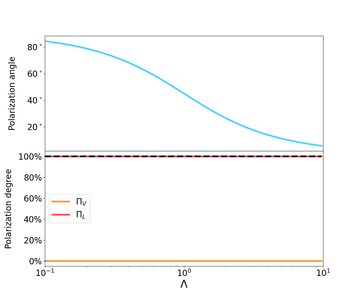
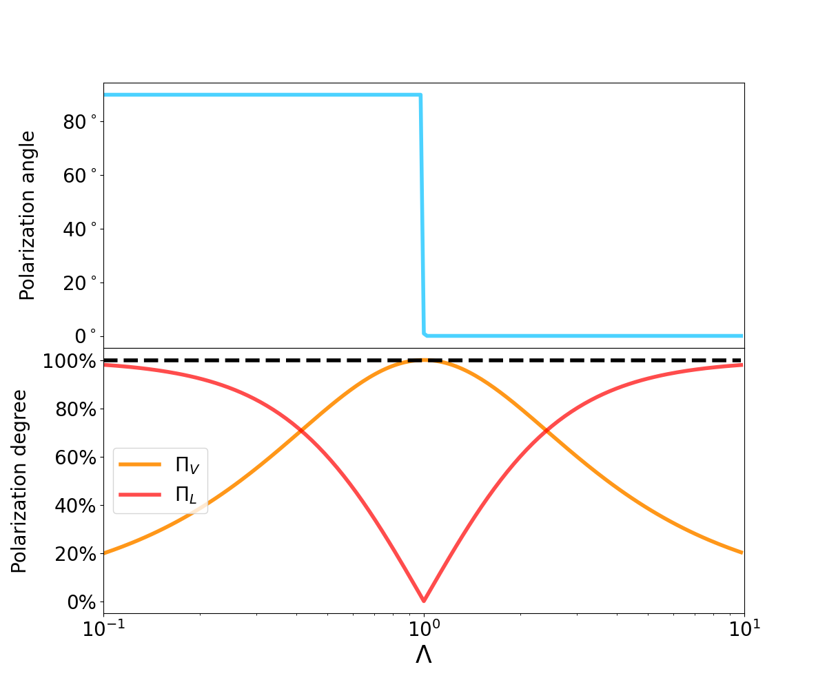
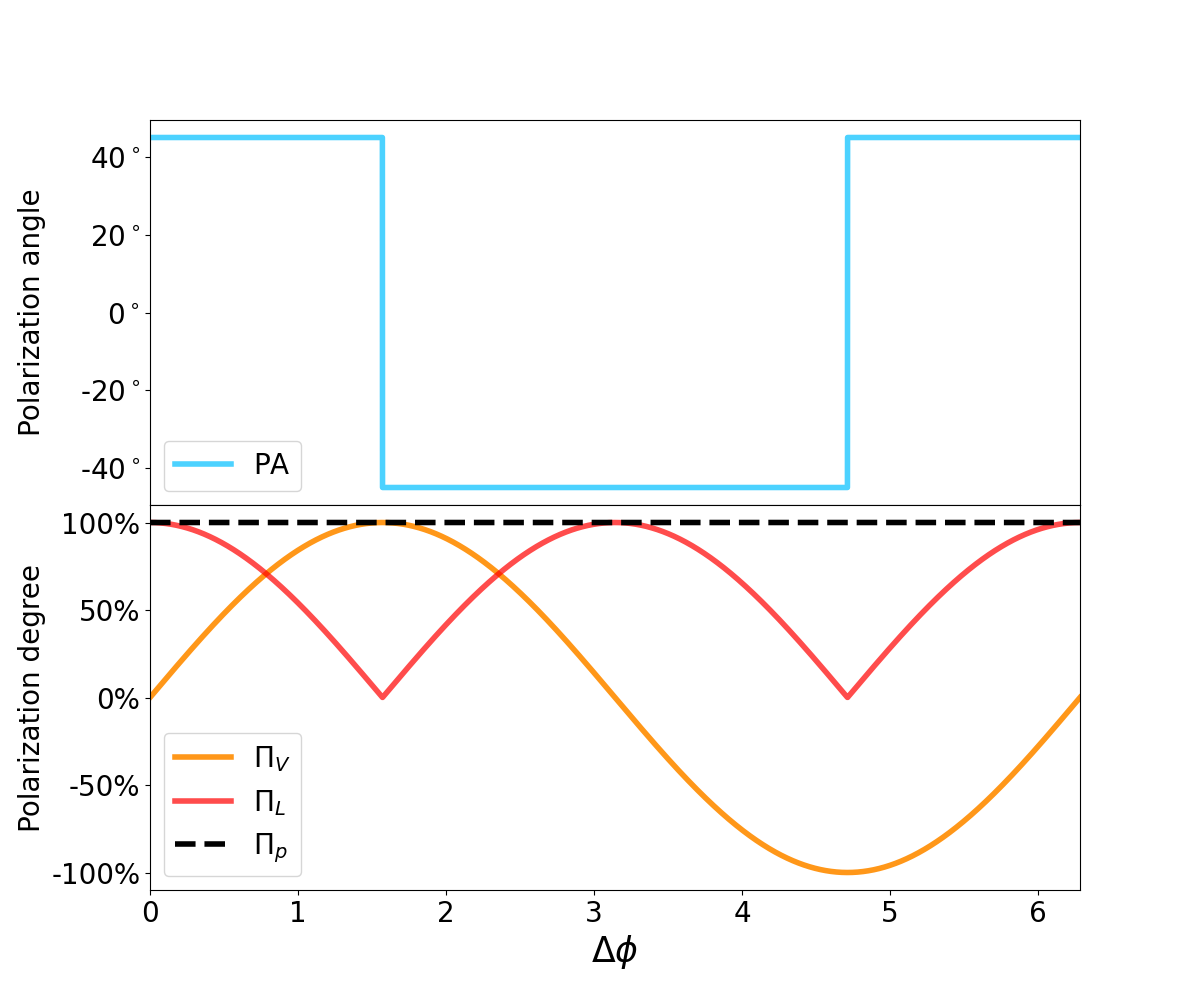
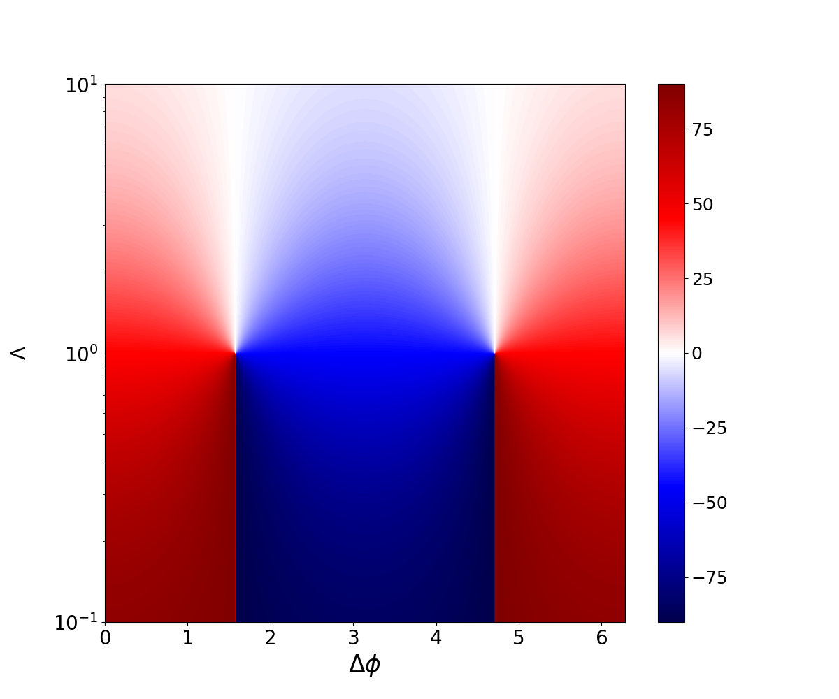
Figure 1: The polarization properties of the superposed waves after coherent superposition. Upper panel: PA and polarization degree as a function of amplitude ratio $\Lambda$ for $\Delta\phi=0$ (upper left) and $\Delta\phi=\pi/2$ (upper right). Two waves are initially 100% linear polarized. Lower left: PA and polarization degree as a function of relative phase $\Delta\phi$ with a fixed value of $\Lambda=1$. Lower right: The value of PA as a function of $\Lambda$ and $\Delta\phi$.

Coherent superposition means the wave trains are overlapped along the LOS, thus one can linearly add the electric fields and then calculate the Stokes parameters. Thus the total orthogonal electric fields along $x$-axis and $y$-axis can be written as

$$E_{1}=E_{1x}+E_{2x}=\varepsilon_{1}\cos\theta_{1}e^{i\phi_{1x}}+\varepsilon_{2}\cos\theta_{2}e^{i\phi_{2x}}.$$ (6)

$$E_{2}=E_{1y}+E_{2y}=\varepsilon_{1}\sin\theta_{1}e^{i\phi_{1y}}+\varepsilon_{2}\sin\theta_{2}e^{i\phi_{2y}}.$$ (7)

The general expression of four Stokes parameters can be calculated as

$$I=\frac{1}{2}(E_{1\rm Re}^{2}+E_{1\rm Im}^{2}+E_{2\rm Re}^{2}+E_{2\rm Im}^{2}),$$ (8)

$$Q=\frac{1}{2}[E_{1\rm Re}^{2}+E_{1\rm Im}^{2}-(E_{2\rm Re}^{2}+E_{2\rm Im}^{2})],$$ (9)

$$U=E_{\rm 1Re}E_{\rm 2Re}+E_{\rm 1Im}E_{\rm 2Im},$$ (10)

$$V=E_{\rm 1Re}E_{\rm 2Im}-E_{\rm 1Im}E_{\rm 2Re},$$ (11)

where

$$E_{1\rm Re}=\varepsilon_{1}\cos\theta_{1}\cos\phi_{1x}+\varepsilon_{2}\cos\theta_{2}\cos\phi_{2x},$$ (12)

$$E_{1\rm Im}=\varepsilon_{1}\cos\theta_{1}\sin\phi_{1x}+\varepsilon_{2}\cos\theta_{2}\sin\phi_{2x},$$ (13)

$$E_{2\rm Re}=\varepsilon_{1}\sin\theta_{1}\cos\phi_{1y}+\varepsilon_{2}\sin\theta_{2}\cos\phi_{2y},$$ (14)

$$E_{2\rm Im}=\varepsilon_{1}\sin\theta_{1}\sin\phi_{1y}+\varepsilon_{2}\sin\theta_{2}\sin\phi_{2y}.$$ (15)

For simplicity, we take $\theta_{1}=0$ and $\theta_{2}=\pi/2$ to consider two 100% linear polarized waves and the two electric fields are perpendicular to each other, i.e. they are orthogonal modes. The superposed wave polarization depends on the relative phase $\Delta\phi$ of the two waves. The corresponding Stokes parameters can be calculated as

$$I=\frac{1}{2}(\varepsilon_{1}^{2}+\varepsilon_{2}^{2}),\ Q=\frac{1}{2}(\varepsilon_{1}^{2}-\varepsilon_{2}^{2}),$$ (16)

$$U=\varepsilon_{1}\varepsilon_{2}\cos\Delta\phi,\ V=\varepsilon_{1}\varepsilon_{2}\sin\Delta\phi.$$

where $\Delta\phi=\phi_{2y}-\phi_{1x}$ is the phase difference between the two waves. The linear and circular polarization degrees can be calculated as

$$\Pi_{L} =\frac{1}{\Lambda^{2}+1}\sqrt{(\Lambda^{2}-1)^{2}+4\Lambda^{2}\cos^{2}\Delta\phi},$$ (17)

and

$$\Pi_{V}=\frac{2\Lambda}{\Lambda^{2}+1}\sin\Delta\phi,$$ (18)

where $\Lambda=\varepsilon_{1}/\varepsilon_{2}$ is the ratio of the two waves amplitude. It should be pointed out that the total polarization degree is always conserved for the coherent superposition case, i.e. $\Pi_{p}=\sqrt{\Pi_{L}^{2}+\Pi_{V}^{2}}=100\%$. The PA can be expressed as

$${\rm PA}=\frac{1}{2}\arctan\frac{2\Lambda\cos\Delta\phi}{\Lambda^{2}-1}.$$ (19)

One can see that when the two waves amplitude is comparable, i.e. $\Lambda=1$, and the relative phase is $\Delta\phi=\pi/2$, then the Stokes parameter $Q=0$ and the sign of $U/Q$ changes, i.e. PA 90-degree jump can occur. Most importantly, $\Pi_{L}=0$ and $\Pi_{V}=100\%$.

Figure 1 shows some results of coherent superposition. In the upper left panel, we consider two 100% linearly polarized waves superposed with the same phase ($\Delta\phi=0$) but different amplitude ratio $\Lambda$. As expected, since the two modes are not orthogonal, no PA jump occurs. PA swing can be observed with varying $\Lambda$ as the relative importance of the two modes varies. The PA can vary by $90^{\circ}$ but no abrupt jump is seen. In the upper right panel of Figure 1, we still consider two 100% linear polarized waves but with a phase difference of $\Delta\phi=\pi/2$. One can see that a $90^{\circ}$ PA jump is observed as $\Lambda=1$. Accompanied with the jump, $\Pi_{L}$ reaches minimum and $\Pi_{V}$ reaches maximum so that the total polarization degree $\Pi_{p}$ is conserved.

Fixing $\Lambda=1$, we present the PA and polarization degrees as a function of phase difference $\Delta\phi$ in the lower left panel of Figure 1. We obtain the same conclusion that the PA jump can occur when the two waves have same amplitude ($\Lambda=1$) but with phase difference $\Delta\phi=\pi/2$ or $3\pi/2$, at which the superposed waves have a nearly 100% circular polarization. It should be pointed out that when one wave amplitude is much greater or smaller than the other wave ($\Lambda\gg 1$ or $\Lambda\ll 1$), PA jumps cannot occur and the polarization mode is nearly $\sim 100\%$ linear. PA as a function of both $\Lambda$ and $\Delta\phi$ is presented in the lower right panel of Figure 1. Again, one can see that the superposed waves are 100% circular polarized at $\Delta\phi=\pi/2$ and $\Delta\phi=3\pi/2$ when $\Lambda=1$, accompanied by a $90^{\circ}$ PA jump. Our conclusions on PA jumps are also valid for other arbitrary values of $\theta_{1}$ and $\theta_{2}$.

2.2 Incoherent superposition

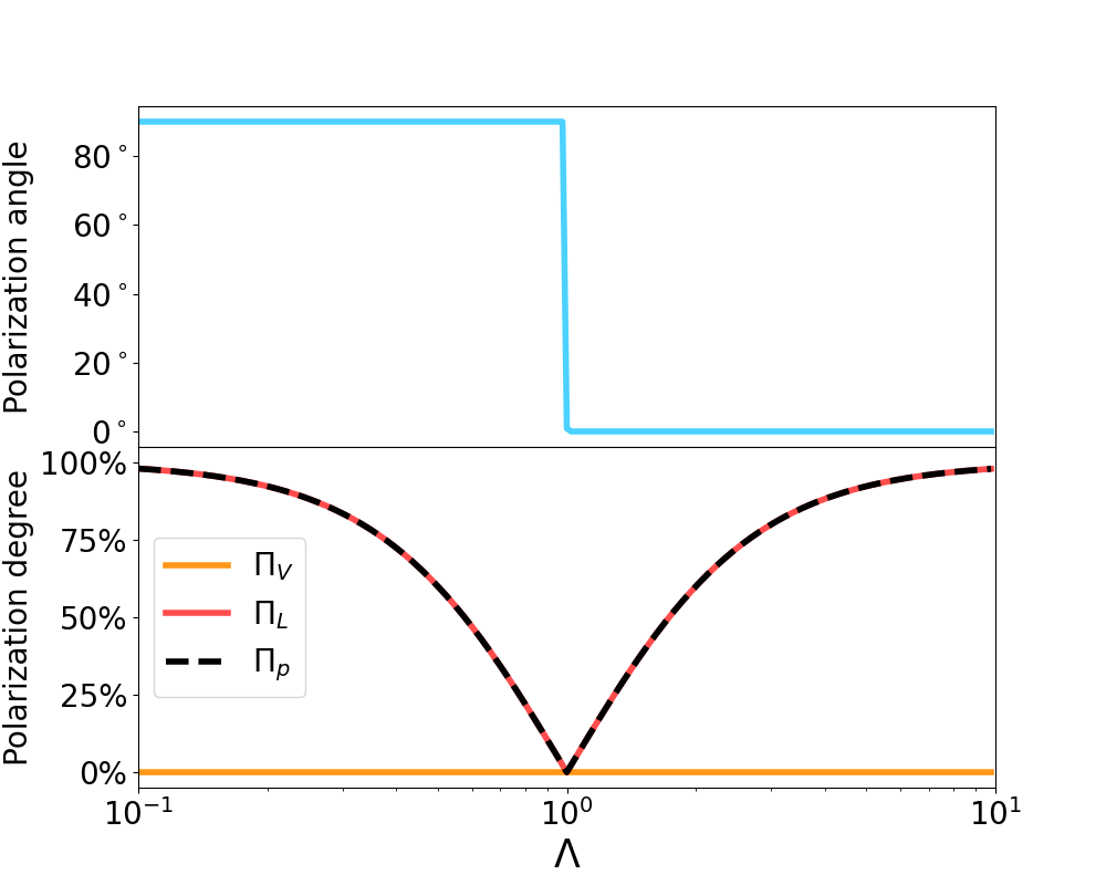
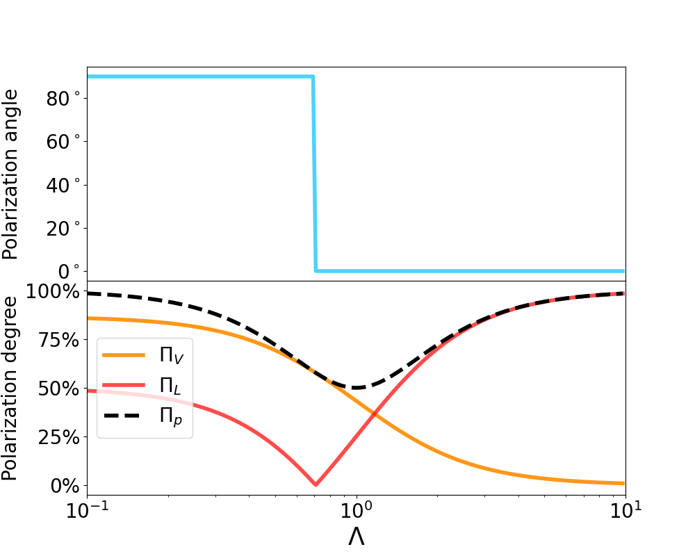
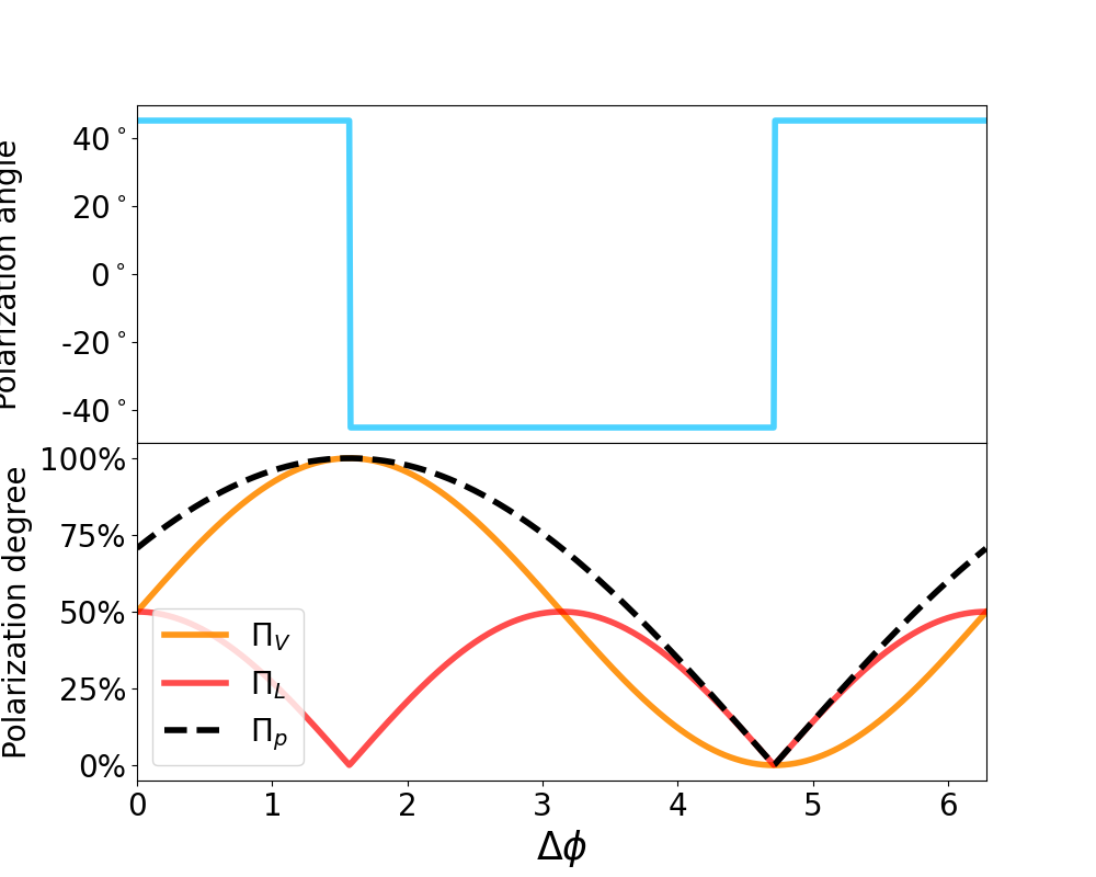
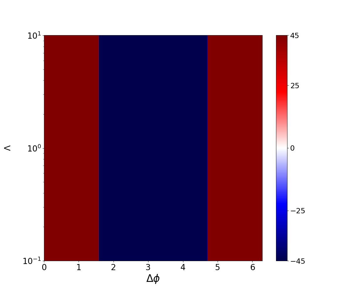
Figure 2: The polarization properties of the superposed waves after incoherent superposition. Upper panel: PA and polarization degree as a function of amplitude ratio $\Lambda$ for $\theta_{1}=0$, $\theta_{2}=\pi/2$ and $\Delta\phi_{1}=\Delta\phi_{2}=0$ (upper left). $\theta_{1}=0$, $\theta_{2}=\pi/3$, $\Delta\phi_{1}=0$ and $\Delta\phi_{2}=\pi/2$ (upper right). Lower left: PA and polarization degree as a function of relative phase $\Delta\phi$ with a fixed value of $\Lambda=1$, $\theta_{1}=\theta_{2}=\pi/4$ and $\Delta\phi_{1}=\pi/2$ (lower left). The value of PA as a function of $\Lambda$ and $\Delta\phi$ for $\theta_{1}=\theta_{2}=\pi/4$ and $\Delta\phi_{1}=\pi/2$ (lower right).

Incoherent superposition occurs when the radiations along different LOSs are produced from very different emission regions or separated due to propagation effects. The observer detects the two waves independently, so that the Stokes parameters rather than the electric fields are summed up linearly. For the first wave (Equation (1)), the Stokes parameters can be written as

$$I_{1}=\frac{1}{2}\varepsilon_{1}^{2}, Q_{1}=\frac{1}{2}\varepsilon_{1}^{2}(\cos^{2}\theta_{1}-\sin^{2}\theta_{1}),$$ (20)

$$U_{1}=\varepsilon_{1}^{2}\sin\theta_{1}\cos\theta_{1}\cos\Delta\phi_{1}, V_{1}=\varepsilon_{1}^{2}\sin\theta_{1}\cos\theta_{1}\sin\Delta\phi_{1},$$

where $\Delta\phi_{1}=\phi_{1y}-\phi_{1x}$. For the second wave (Equation (2)), the Stokes parameters can be written as

$$I_{2}=\frac{1}{2}\varepsilon_{2}^{2}, Q_{2}=\frac{1}{2}\varepsilon_{2}^{2}(\cos^{2}\theta_{2}-\sin^{2}\theta_{2}),$$ (21)

$$U_{2}=\varepsilon_{2}^{2}\sin\theta_{2}\cos\theta_{2}\cos\Delta\phi_{2}, V_{2}=\varepsilon_{2}^{2}\sin\theta_{2}\cos\theta_{2}\sin\Delta\phi_{2},$$

where $\Delta\phi_{2}=\phi_{2y}-\phi_{2x}$. Therefore, the Stokes parameters of the waves due to incoherent superposition can be calculated as

$$I=I_{1}+I_{2}=\frac{1}{2}\varepsilon_{1}^{2}+\frac{1}{2}\varepsilon_{2}^{2}.$$ (22)

$$Q=Q_{1}+Q_{2}=\frac{1}{2}\varepsilon_{1}^{2}(\cos^{2}\theta_{1}-\sin^{2}\theta_{1})+\frac{1}{2}\varepsilon_{2}^{2}(\cos^{2}\theta_{2}-\sin^{2}\theta_{2}).$$ (23)

$$U=U_{1}+U_{2}=\varepsilon_{1}^{2}\sin\theta_{1}\cos\theta_{1}\cos\Delta\phi_{1}+\varepsilon_{2}^{2}\sin\theta_{2}\cos\theta_{2}\cos\Delta\phi_{2}.$$ (24)

$$V=V_{1}+V_{2}=\varepsilon_{1}^{2}\sin\theta_{1}\cos\theta_{1}\sin\Delta\phi_{1}+\varepsilon_{2}^{2}\sin\theta_{2}\cos\theta_{2}\sin\Delta\phi_{2}.$$ (25)

The linear and circular polarization degree can be calculated as

$$\Pi_{L}=\frac{2}{\varepsilon_{1}^{2}+\varepsilon_{2}^{2}}\sqrt{Q^{2}+U^{2}},$$ (26)

and

$$\Pi_{V}=\frac{2}{\Lambda^{2}+1}[\Lambda^{2}\sin\theta_{1}\cos\theta_{1}\sin\Delta\phi_{1}+\sin\theta_{2}\cos\theta_{2}\sin\Delta\phi_{2}],$$ (27)

and the PA can be calculated as

$${\rm PA}=\frac{1}{2}\arctan\frac{2\Lambda^{2}\sin\theta_{1}\cos\theta_{1}\cos\Delta\phi_{1}+2\sin\theta_{2}\cos\theta_{2}\cos\Delta\phi_{2}}{\Lambda^{2}(\cos^{2}\theta_{1}-\sin^{2}\theta_{1})+\cos^{2}\theta_{2}-\sin^{2}\theta_{2}}.$$ (28)

We first consider the superposition of two 100% linearly polarized waves, i.e. $\Delta\phi_{1}=\Delta\phi_{2}=0$. When the two waves have the same polarization angle, i.e. $\theta_{1}=\theta_{2}=0$, the superposed wave is still 100% linearly polarized and there is no PA jump. In order to produce a PA jump, we assume that the two waves are orthogonal modes before superposition, i.e. $\theta_{1}=0$ and $\theta_{2}=\pi/2$, and two 100% linearly polarized waves are assumed with $\Delta\phi_{1}=\Delta\phi_{2}=0$. We present PA and polarization degrees as a function of $\Lambda$ in the upper left panel of Figure 2. One can see that the PA jump occurs when $\Lambda=1$ since the Stokes-$Q$ equals zero at the jump point and the sign also changes.

Next, we explore the superposition of two waves with different polarization properties. We assume that the first wave is 100% linearly polarized with $\theta_{1}=0$ and $\Delta\phi_{1}=0$, and that the second wave is elliptically polarized with $\theta_{2}=\pi/3$ and $\Delta\phi_{2}=\pi/2$. We present PA and polarization degrees as a function of $\Lambda$ in the upper right panel of Figure 2. One can see that the PA jump occurs not exactly at $\Lambda=1$ which is different from the coherent superposition case. The linear polarization degree reaches the minimum value and the total polarization degree is not conserved. In the lower left panel of Figure 2, one can see that PA jumps occur at $\Delta\phi=\pi/2$ and the linear polarization degree reaches the minimum value for $\Lambda=1$. In the lower right panel of Figure 2, we present PA as a function of both $\Lambda$ and $\Delta\phi$. One can see that the value of PA is constant for a constant $\Delta\phi$ regardless of $\Lambda$ and jumps can occur at $\Delta\phi=\pi/2$ or $\Delta\phi=3\pi/2$.

To summarize the main results of this section, we find that the polarization properties due to two waves superposition can potentially account for the observed PA jumps under certain conditions. Both coherent and incoherent superposition can generate PA jumps, with the linear polarization degree always reaching the minimum value. For the coherent superposition case, the total polarization degree is conserved, so that the circular polarization reaches the maximum value when a PA jump occurs. On the other hand, for the incoherent superposition case, the total polarization degree does not always conserve to maintain 100%. Thus, the maximum value of the circular polarization degree is not exactly at the PA jump time.

3 GENERIC OBSERVATIONAL CONSTRAINTS

So far, we have not discussed PA variation/jump as a function of time, as is observed in the three FRB bursts (and also in some radio pulsars). In order to account for the observed jumps within the milliseconds timescale, some very generic constraints on the models can be placed. This is the purpose of this section. Various possible mechanisms to produce PA orthogonal jumps and their plausibility are presented in Figure 3.

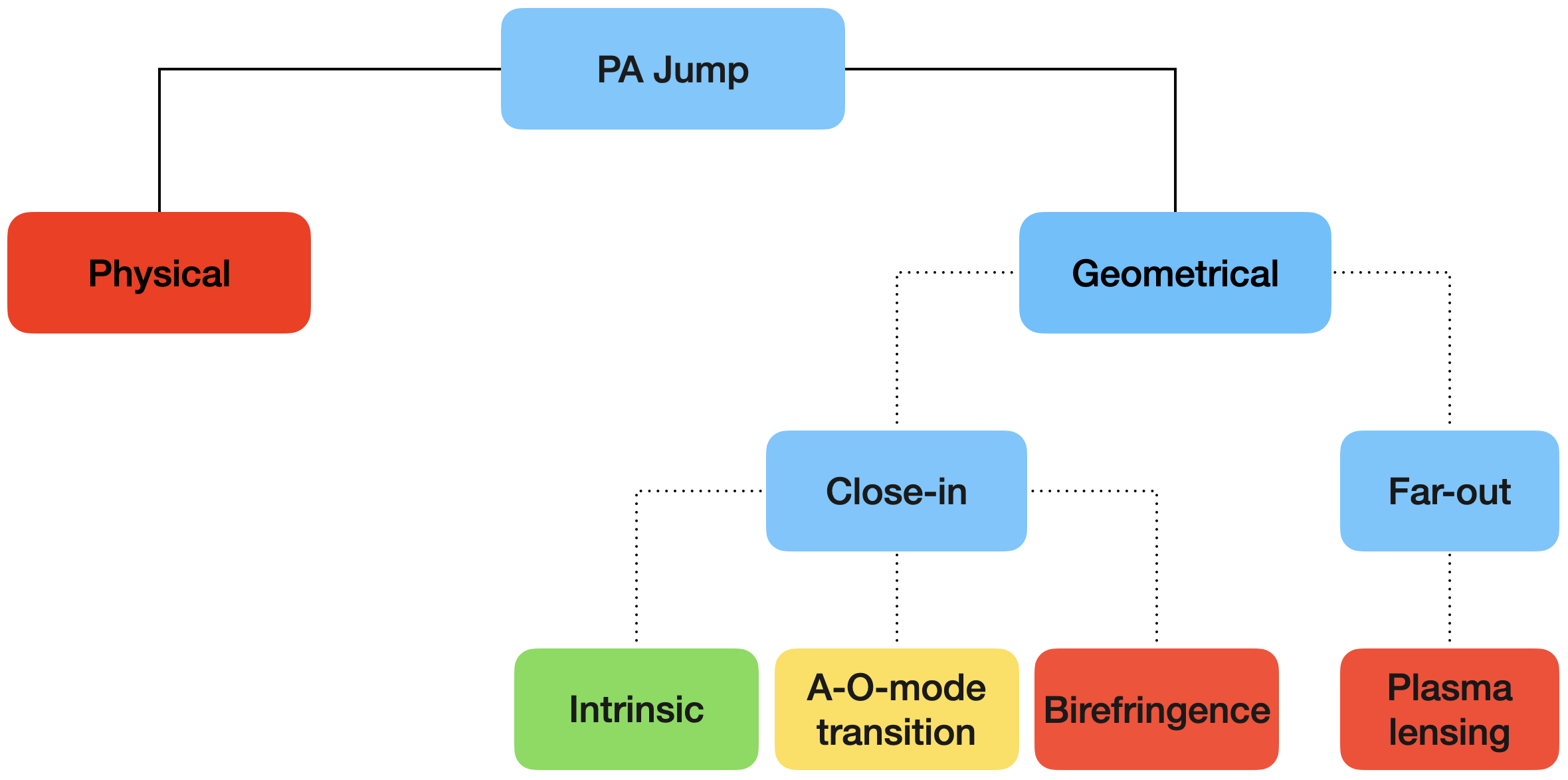
Figure 3: General physical and geometrical processes to generate polarization angle jumps of FRBs discussed in Section 3. For each process, close-in (inside the magnetosphere) and far-away (outside the magnetosphere) models are investigated. The favored processes are marked as green, possible process is marked as yellow and the disfavored processes are marked as red.

3.1 Physical vs. Geometrical Scenarios

To observe a sudden change of PA within the milliseconds timescale, one can envisage two distinct scenarios. The first scenario is that there is an intrinsic change of the physical properties of the emitter within such a short timescale, which we call the physical scenario. Another is to introduce a geometric effect, with the line of sight sweeping a rotating object, and the sudden jump in PA occurs as the LOS goes across a region where the physical conditions change. We call this second scenario the geometric scenario.

We argue that the physical scenario is extremely unlikely. In order for the PA of the emission mode to suddenly jump by $90^{\circ}$ within milliseconds, one requires that the magnetic configuration in the emission region undergo such an abrupt change during such a short period of time. Such a scenario has never been realized and even envisaged in any FRB emission models, invoking either magnetospheric emission or maser emission in relativistic shocks. The ms-duration also places a tight limit of the size of the emission region, which is

$$l_{\rm em}=c\delta t=(3\times 10^{7}\ {\rm cm})\ \delta t_{-3},$$ (29)

for a non-relativistic emitter, where $\delta t$ is the typical duration of the jump (which is normalized to millisecond). Furthermore, even if the magnetic field undergoes a global reconfiguration in such a short period of time, it is very contrived to allow the PA jump by $90^{\circ}$. One may also envisage a sudden change of the particle spatial distribution or radiation mechanism to account for the jump without a significant change of the magnetic configuration. However, the required change is also highly contrived and there is no known physics to trigger such a change.

We therefore conclude that the origin of the PA orthogonal jump very likely invokes a geometric scenario, with a rotating object viewed by a varying viewing angle and different emission modes dominating in different viewing directions.

3.2 Close-in vs. Far-out

Within the geometric scenario, one can generally discuss two general types models. The first type invokes magnetospheric emission from an FRB central engine, which is called close-in or pulsar-like models; the second type invokes relativistic shocks way outside of the light cylinder of the engine, which is called far-out or GRB-like models. We argue that the observational data strongly disfavors the far-out models.

First, within the far-out models, because the emission region is far from the central engine and well beyond the light cylinder, the emitter is not undergoing significant rotation. The LOS does not sweep across significantly different emission regions within milliseconds. More specifically, the synchrotron maser model (Plotnikov & Sironi, 2019; Metzger et al., 2019; Sironi et al., 2021) can produce both X-mode and O-mode emissions, but the wave amplitude ratio between the two modes is found in the 3D PIC simulation to be dominated by the X-mode, i.e. $|{E_{\rm X}}/{E_{\rm O}}|\sim 1.6\sqrt{\sigma}\gg 1$ (Sironi et al., 2021), where $\sigma\gg 1$ is the magnetization factor, which is required to be much greater than unity to allow the mechanism to produce the high brightness temperature as observed in FRBs. As a result, even if the LOS can sweep different emission regions, the emission is always dominated by the X-mode. without a contrived sudden spatial change of the magnetic configuration (which is never observed in numerical simulations), the sudden orthogonal jump is impossible.

Another possibility for producing an orthogonal jump from far away distances is through plasma lensing. In particular, it has been shown (Er et al., 2023) that with a proper setup, a plasma lens can produce distinct cusps across which a jump in the polarization mode can happen. However, the chance of having the LOS sweeping right into these cusps during FRB bursts is extremely low. Consider the proper motion velocity of a magnetar with $v_{\rm pro}=10^{7}\ \rm cm\ s^{-1}$. Within the typical time duration of PA jumps $\delta t\sim 1\ \rm ms$, the corresponding transverse length scale is $l_{\perp,\rm pro}\simeq v_{\rm pro}\delta t=(10^{4}\ {\rm cm})\ v_{\rm pro,7}\delta t_{-3}$. Notice that three PA jump events were observed in over 2000 bursts (1863 bursts in the first episode and more than 600 bursts in the second episode) from FRB 20201124A are reported during the time span of $\sim 2.5$ months (Niu et al., 2024). The total time duration of $\sim 2000$ FRBs may be estimated as $\Delta T\sim 2000\Delta t_{\rm frb}=(2\ {\rm s})\ \Delta t_{\rm frb,-3}$, which is related to the distance traveled by the proper motion of the FRB engine

$$l_{\perp,\rm obs}\simeq v_{\rm pro}\Delta T\simeq(2\times 10^{7}\ {\rm cm})\ v_{\rm pro,7}\Delta T_{0.3}.$$ (30)

One can then derive a number density of the plasma lens normal to the line of sight

$$n_{l}\simeq\frac{3}{l_{\perp,\rm obs}}\simeq(1.5\times 10^{-7}\ {\rm cm^{-1}})\ v_{\rm pro,7}^{-1}\Delta T_{0.3}^{-1}.$$ (31)

This density is way too high for plasma lenses. Even if one considers that these lenses are placed one by one without any spacing (which is realistically impossible because a special arrangement of the plasma properties is needed to make a lens), the linear density is still smaller than Equation (31). This can be proved by estimating the Fresnel angle ($\theta_{\rm F}$), which is defined as the angular position on the lens plane where the radio wave from the source propagating through this point would induce an additional geometric phase difference of $2\pi$ relative to a straight line trajectory from the source to the observer. It can be estimated as

$$d_{\rm F}=\left(\frac{2\lambda d_{\rm SL}d_{\rm LO}}{d_{\rm SO}}\right)^{1/2} \simeq\left({2\lambda d_{\rm SL}}\right)^{1/2}$$ (32)

$$\simeq(2.4\times 10^{7}\ {\rm cm})\ \nu_{9}^{1/2}d_{\rm SL,13}^{1/2},$$

where $d_{\rm LO}$ is from the lens to the observer, $d_{\rm SO}$ is from the FRB source to the observer, and $d_{\rm SL}$ is the distance from the FRB source to the lens, which is normalized to a typical distance of $10^{13}$ cm. This gives a maximum linear number density for lenses

$$n_{\rm l,max}\sim n_{\rm F}\sim 1/d_{\rm F}\simeq 4.2\times 10^{-8},$$ (33)

which is smaller than $n_{l}$ definde in Equation (31). We conclude that PA jumps cannot be produced through plasma lensing outside the magnetosphere of the central engine.

4 Physical scenarios for orthogonal jumps inside the magnetosphere

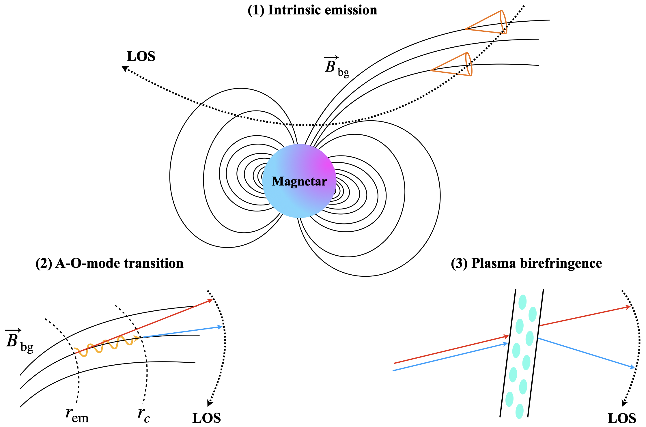
Figure 4: A cartoon figure for three scenarios to produce PA jumps of FRBs including (1) intrinsic emission (upper panel), (2) A-O-mode transition (lower left) and (3) Plasma birefringence (lower right) discussed in geometric effects. In all panels, the red line and blue line denote two different orthogonal modes of FRBs. The curved back dashed arrow represents the trajectory of the LOS, with its direction indicating how the LOS evolves over time. The solid black curves denote background magnetic field ($\vec{B}_{\rm bg}$) in both (1) and (2). In (1), the LOS in the azimuthal direction sweeps from an O-mode-dominated region to an X-mode dominated region. In (2), two dashed black lines denote the emission radius ($r_{\rm em}$) and critical transition radius ($r_{c}$), respectively. In (3), the cyan clumps represent plasma located ahead of the FRBs.

The generic constraints presented in the last section leave the geometric scenarios of the magnetospheric origin as the most plausible ones for orthogonal jumps. In this section, we investigate in detail the three most relevant magnetospheric processes, as indicated in Figure 4:

1. The two orthogonal modes (X-mode and O-mode) are intrinsically produced. The relative dominance of these two modes depends on the viewing angle and emission geometry. As the LOS sweeps across different emission regions, PA jumps occur naturally when the dominant mode switches between the X-mode and O-mode.

2. A-O mode transition: The emission is produced in the high-density plasma region, with the X-mode escaping freely in straight lines, while the orthogonal mode is the Alfvén mode that propagates along the magnetic field lines. As Alfvén waves finally escape in a low-density region as O-mode waves, they naturally beam toward a different region than the X-mode waves. As the LOS sweeps, it will first detect the X-mode and later the O-mode, or vice versa. A PA jump would be observed as the LOS sweeps across regions dominated by the two different modes.

3. Plasma birefringence: If a wave with mixed X- and O-mode reaches a plasma region with an incident angle different from $90^{\circ}$, the two modes will be refracted to different directions. A PA jump would happen if the LOS can sweep across regions dominated by the two different modes.

4.1 Intrinsic emission mechanisms

Some intrinsic radiation mechanisms can produce two orthogonal modes (e.g. X- and O- modes). In order to detect a sudden jump between the two modes, one requires two conditions: (1) the medium should be transparent to both modes; and (2) the two modes should have comparable amplitudes at the transition time.

Before discussing the detailed intrinsic mechanisms, we first consider the condition for the transparency of the two modes. When the wave frequency exceeds the plasma frequency, both for X-mode and O-mode, electromagnetic waves can propagate freely such as in vacuum. When the frequency is below the plasma frequency, the X-mode is in the form of fast magnetosonic waves, which can still propagate as long as they remain in the linear regime, where the MHD description remains valid. However, the O-mode cannot propagate, which can be only converted from the Alfvén mode at a critical radius $r_{c}$ radius defined by the condition $\omega^{\prime}=\omega_{p}^{\prime}$ in the comoving frame of the relativistic plasma. The transition radius for Alfvén waves (to O mode) and for fast magnetosonic waves (to X mode) can be calculated as

$$r_{c} =\left(\frac{\xi B_{\star}R_{\star}^{3}q{\cal D}^{2}}{cP\gamma m_{e}\pi\nu^{2}}\right)^{1/3}$$ (34)

$$\simeq\left\{\begin{array}[]{ll}&(1.3\times 10^{8}\ {\rm cm})\ \xi^{1/3}B_{\star,15}^{1/3}R_{\star,6}\gamma_{2}^{1/3}P^{-1/3}\nu_{9}^{-2/3},\\ &~~~~~~~~~~~~~~~~~~~~~~{\rm A~mode\rightarrow O~mode},\\ &(5.2\times 10^{7}\ {\rm cm})\ \xi^{1/3}B_{\star,15}^{1/3}R_{\star,6}\gamma_{2}^{-1/3}P^{-1/3}\nu_{9}^{-2/3}\left(\frac{{\cal D}}{50}\right)^{2/3},\\ &~~~~~~~~~~~~~~~~~~~~~~{\rm F~mode\rightarrow\ X~mode},\end{array}\right.$$

where $\xi$ is the multiplicity, $\nu=\omega/2\pi$ is the FRB frequency, $\gamma$ is the Lorentz factor of the relativistic plasma, ${\cal D}=1/[\gamma(1-\beta\cos\theta)]$ is the Doppler factor, which is adopted as ${\cal D}=2\gamma$ for Alfvén waves with $\theta=0$. For fast magnetosonic waves, $\cal D$ is normalized to 50, which corresponds to $\theta=1^{\circ}$ for $\gamma=100$.

The second condition, i.e. the X- and O-modes have comparable amplitudes, depends on the concrete radiation mechanisms. In the following, we discuss the two widely discussed radiation mechanisms, curvature radiation (CR) and inverse Compton scattering (ICS), in detail.

4.1.1 Coherent curvature radiation

A widely studied radiation mechanism for FRBs within the inner magnetar magnetosphere is the coherent curvature radiation emitted by charged bunches (Kumar et al., 2017; Lu et al., 2020; Kumar & Bošnjak, 2020). We consider one single charged bunch moving along the background magnetic field line, the amplitudes of orthogonal modes via curvature radiation are given by (Jackson, 1998)

$$E_{\rm X}(\omega)\simeq\frac{i2\rho}{\sqrt{3}c}\left(\frac{1}{\gamma^{2}}+\theta_{v}^{2}\right)K_{2/3}(\varsigma)$$ (35)

which describes the X-mode amplitude, and

$$E_{\rm O}(\omega)\simeq\frac{2\rho}{\sqrt{3}c}\theta_{v}\left(\frac{1}{\gamma^{2}}+\theta_{v}^{2}\right)^{1/2}K_{1/3}(\varsigma)$$ (36)

which describes the O-mode amplitude. Here, $\rho$ denotes the curvature radius, $\theta_{v}$ is the viewing angle between the LOS and the particle motion direction, $K_{\nu}(\varsigma)$ is the modified Bessel function and the parameter $\varsigma=\omega\rho(1/\gamma^{2}+\theta_{v}^{2})^{3/2}/3c$ is defined. The amplitude ratio of the two orthogonal modes can be calculated as

$$\left|\frac{E_{\rm X}}{E_{\rm O}}\right|=\frac{1}{\theta_{v}}\left(\frac{1}{\gamma^{2}}+\theta_{v}^{2}\right)^{1/2}\frac{K_{2/3}(\varsigma)}{K_{1/3}(\varsigma)}\simeq 1\ \ {\rm for}\ \ \gamma\theta_{v}\gg 1.$$ (37)

Notice that the values of $K_{2/3}(\varsigma)$ and $K_{1/3}(\varsigma)$ are nearly the same. We present the wave amplitude ratio of X-mode to O-mode in the left panel of Figure 5. When $\theta_{v}=0$ (on-axis case), the electron can only produce 100% linearly polarized X-mode waves since $E_{\rm O}(\omega)=0$. In order to produce non-negligible O-mode waves, one needs to observe the emitting bunch at an off-axis viewing angle ($\theta_{v}\neq 0$). We note that the ratio $E_{\rm X}/E_{\rm O}>1$ when $\theta_{v}<1/\gamma$ and approaches unity when $\theta_{v}>1/\gamma$, i.e. the amplitude ratio of X-mode to O-mode is always greater than unity.

In order to obtain the temporal evolution of PA, we need to find out the relation between the amplitude ratio and time. The viewing angle dependence on observation time as the magnetar spins can be written as

$$\theta_{v}(t)=\frac{v_{\rm rot}t}{r_{\rm em}}+\theta_{v,0}=\frac{2\pi t}{P},$$ (38)

where the initial viewing angle $\theta_{v,0}=0$ is chosen at $t=0$. The amplitude ratio of two modes depends on $\theta_{v}$, thus it also depends on time as magnetar spins. We present the temporal evolution of PA in the right panel of Figure 5. One can see that PA jumps do not occur solely via intrinsic wave superposition since $E_{\rm X}\gtrsim E_{\rm O}$ is always satisfied for a single charged bunch’s curvature radiation. Observations suggest an incoherent superposition, however, the LOS always observes the X-mode as dominant from all viewing angles, even if it sweeps different bunches at different locations. It is difficult to produce an orthogonal PA jump unless the magnetic configuration switches by $90^{\circ}$, which is difficult to achieve. Thus, additional propagation effects are needed to make the O-mode waves dominant.

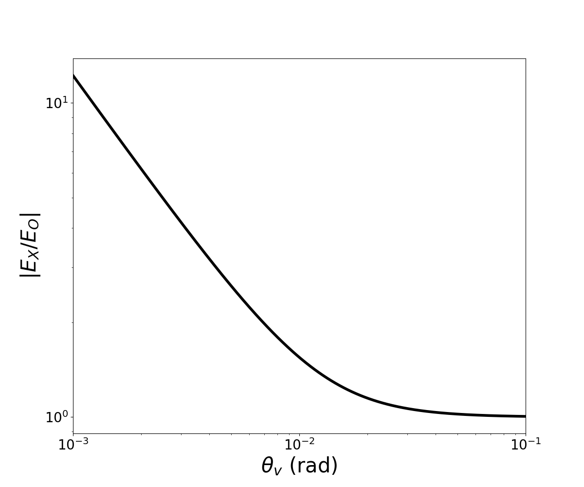
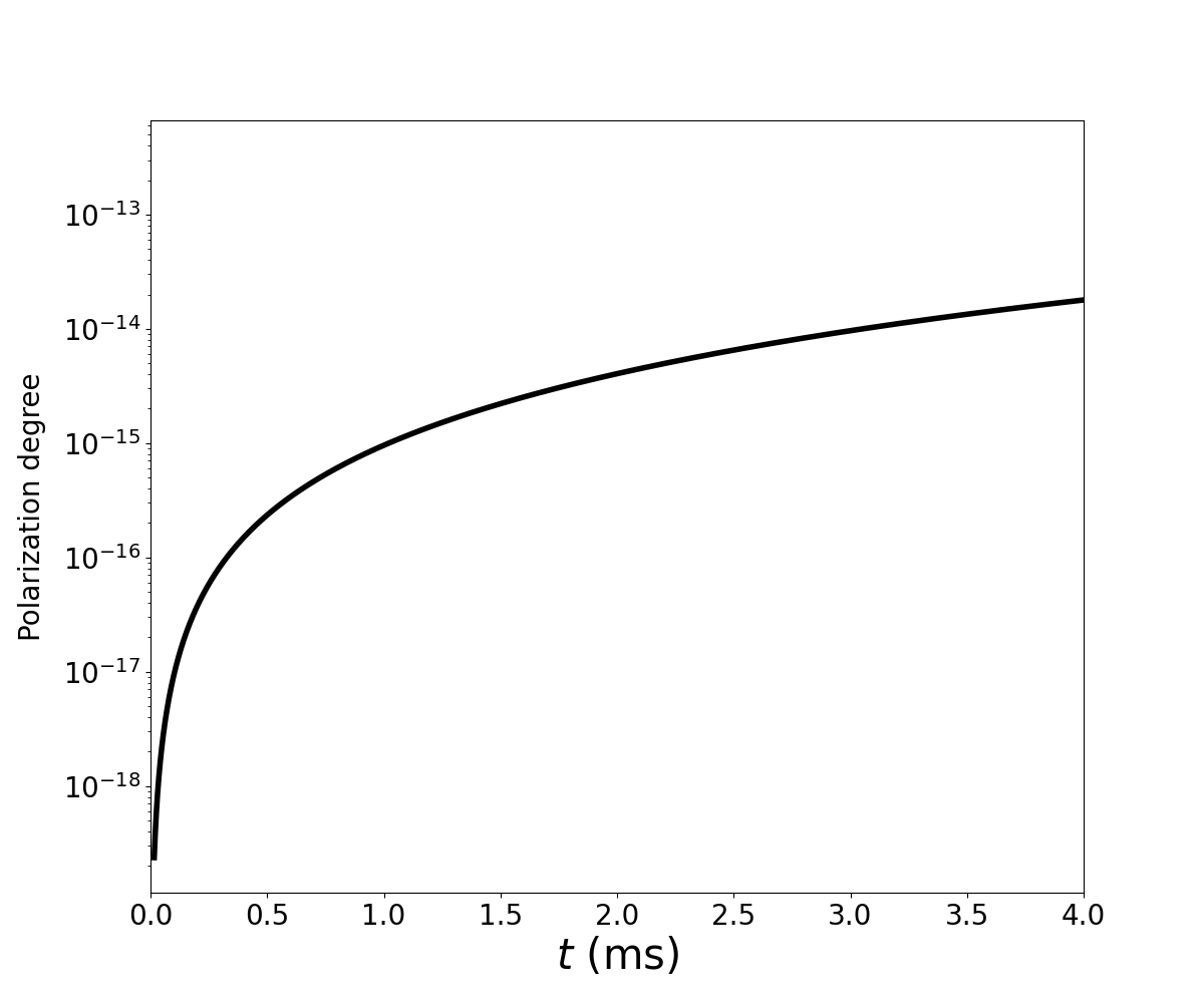
Figure 5: Left panel: The amplitude ratio of X-mode to O-mode as a function of viewing angle $\theta_{v}$ for a single charged bunch’s curvature radiation. Right panel: PA as a function of time via incoherent superposition. Following parameters are adopted: Curvature radius $\rho=10^{7}\ \rm cm$, emission frequency $\nu=1\ \rm GHz$, the Lorentz factor $\gamma=100$ and magnetar spin period $P=1\ \rm s$.

4.1.2 Coherent inverse Compton scattering

The coherent ICS process by charged bunches off $\sim{\rm kHz}$ frequency fast magnetosonic waves produced by the magnetar crust quake in the context of FRBs has been discussed by Zhang (2022) and Qu & Zhang (2024). We define the unit vector of the LOS as $\hat{n}^{\prime}=\sin\theta_{v}^{\prime}\cos\phi_{v}^{\prime}\hat{x}+\sin\theta_{v}^{\prime}\sin\phi_{v}^{\prime}\hat{y}+\cos\theta_{v}^{\prime}\hat{z}$ in the comoving frame of the relativistic charged bunch. The electric field of the scattered waves for one charged particle in the comoving frame is given by (Qu & Zhang, 2024)

$$\vec{E}_{\rm rad}^{\prime} =\frac{q^{2}E_{\rm fmw}^{\prime}\sin(\omega_{i}^{\prime}t^{\prime})}{m_{e}cR^{\prime}}\left(\frac{\omega_{i}^{\prime}}{\omega_{B}^{\prime}}\right)[\cos\phi_{v}^{\prime}\sin\phi_{v}^{\prime}\sin^{2}\theta_{v}^{\prime}\hat{x}$$ (39)

$$-(\cos^{2}\theta_{v}^{\prime}+\cos^{2}\phi_{v}^{\prime}\sin^{2}\theta_{v}^{\prime})\hat{y}+\cos\theta_{v}^{\prime}\sin\phi_{v}^{\prime}\sin\theta_{v}^{\prime}\hat{z}],$$

where $E_{\rm fmw}^{\prime}$ and $\omega_{i}^{\prime}$ are the electric field amplitude and angular frequency of the incident low frequency waves in the comoving frame, respectively. We perform a Lorentz transformation on the electric field, converting it from the comoving frame to the lab frame as

$$\vec{E}_{\rm rad}=\vec{E}_{\rm rad,\parallel}^{\prime}+\gamma(\vec{E}_{\rm rad,\perp}^{\prime}-\vec{\beta}\times\vec{B}^{\prime}),$$ (40)

where the subscripts “$\parallel$” and “$\perp$” denote the parallel and perpendicular components of the radiation electric fields with respect to background magnetic field $\vec{B}_{\rm bg}$. Then the electric fields of X-mode and O-mode in the lab frame can be generally expressed as

$$|\vec{E}_{\rm X}| =|\vec{E}_{\rm rad}\cdot(\hat{n}\times\hat{B}_{\rm bg})|$$ (41)

$$=|E_{x}\sin\phi_{v}\sin\theta_{v}-E_{y}\cos\phi_{v}\sin\theta_{v}|,$$

and

$$|\vec{E}_{\rm O}| =|\vec{E}_{\rm rad}\times(\hat{n}\times\hat{B}_{\rm bg})|$$ (42)

$$=|E_{z}\cos\phi_{v}\sin\theta_{v}\hat{i}+E_{z}\sin\phi_{v}\sin\theta_{v}\hat{j}$$

$$-(E_{x}\cos\phi_{v}\sin\theta_{v}+E_{y}\sin\phi_{v}\sin\theta_{v})\hat{k}|,$$

where the expressions of $E_{x}$, $E_{y}$ and $E_{z}$ are derived in Appendix A. We present the amplitude ratio of X-mode to O-mode waves as a function of the viewing angle ($\theta_{v}$) in the left panel of Figure 6 for different azimuthal angles ($\phi_{v}$). One can see that the X- and O-mode amplitudes could be equivalent at specific viewing angles.

Similarly to the case of curvature radiation, we present the temporal evolution of PA in the right panel of Figure 6 by considering $\phi_{v}=60^{\circ}$. We note that PA jumps occur within millisecond timescales at the transition of the two orthogonal modes. As the magnetar spins, the radiation properties will change in the azimuthal direction. Therefore, we conclude that the ICS mechanism provides a plausible explanation for generating PA jumps via incoherent wave superposition.

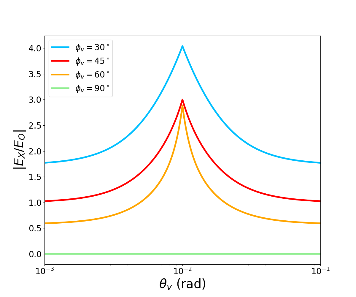
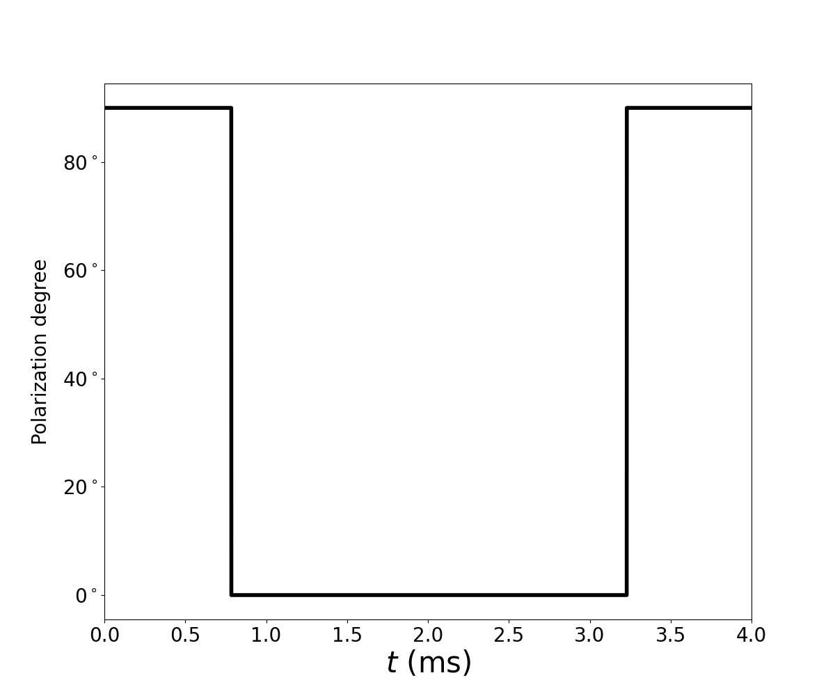
Figure 6: Left panel: The amplitude ratio of X-mode to O-mode as a function of viewing angle $\theta_{v}$ for ICS. Right panel: Polarization angle as a function of time via incoherent superposition. The Lorentz factor $\gamma=100$, magnetar spin period $P=1\ \rm s$ and $\phi_{v}=60^{\circ}$ are adopted for the right panel.

4.1.3 Monster shock

It has been proposed that fast magnetosonic waves entering the nonlinear region can power different types of high-energy transients, including FRBs, in the closed field line region of magnetars (Beloborodov, 2023). 1D PIC simulations of this physical process have shown that only X-mode waves are generated (Vanthieghem & Levinson, 2025). If this is the case, it is impossible to produce waves with comparable X- and O-modes, so orthogonal PA jumps would rule out such models.

4.2 A-O-mode transition

In the second scenario, we consider an emitter deeper in the magnetosphere where the wave frequency is below the plasma frequency in the comoving frame, i.e. $\omega^{\prime}<\omega_{p}^{\prime}$ (or $r_{\rm em}<r_{c}$). In this case, unlike the opposite case where both the O-mode and the X-mode waves can propagate freely (as discussed in Section 4.1), only one of the two orthogonal modes, i.e. the X-mode, or the fast magnetosonic mode (F-mode), can propagate freely. The other mode, i.e. the Alfvén mode polarized in the $\vec{k}-\vec{B}_{\rm bg}$ plane can only propagate along the background magnetic field line.

Suppose that an FRB emitter at an emission radius satisfies $r_{\rm em}<r_{c}$. Fast magnetosonic waves will propagate freely and convert into X-mode waves with the same emission direction at $r=r_{c}$, Alfvén waves, on the other hand, continue change direction and convert into O-mode waves at $r=r_{c}$ and propagate nearly tangentially to the local background magnetic field lines. Thus, the propagation directions of X-mode and O-mode are different when $r>r_{c}$ (see the lower left panel of Figure 4). A line of sight would see an abrupt change when it sweeps from an X-mode-dominated region to an O-mode-dominated region.

The conversion from the Alfvén mode to O-mode needs some justification. This is because if the plasma density drops with radius only mildly, $\omega^{\prime}/\omega_{p}^{\prime}$ would only increases slowly from below and only approaches unity when the wave becomes a plasma-oscillation Langmuir wave, which would be damped. In order to suddenly crossing the $\omega^{\prime}/\omega_{p}^{\prime}=1$ line and reaching the O-mode branch, $\omega^{\prime}_{p}$ needs to drop significantly in the distance scale of the wavelength $\lambda^{\prime}$. We argue that this is marginally possible because the typical size of the plasma bunches that emit FRBs is of the order of $\lambda^{\prime}$. We envisage that the plasma is composed of these clumps with the characteristic spatial scale of $\lambda^{\prime}$ in the comoving frame. At $r_{c}$, A-O-mode transition can occur due to the rapid variation of $\omega^{\prime}/\omega_{p}^{\prime}$ around unity within one wavelength scale.

4.3 Birefringence

When radio waves consisting of two orthogonal modes propagate into a plasma with a distinct refraction index $n>1$ with an oblique angle, the two modes would propagate in different directions after exiting the plasma, resulting the separation of the two orthogonal modes (see the lower right panel of Figure 4).

More generally, for an original FRB wave to undergo refraction, the background medium must exhibit spatial variations, and the $n$ gradient must not be parallel to the wave propagation direction (see the lower right panel of Figure 4).

However, the plasma clumps are moving relativistically along $\vec{B}_{\rm bg}$ and we must consider the $n$ variation in the lab frame. For relativistic motion, the refractive index in the lab frame can be calculated as (see Appendix B for a derivation)

$$n=\frac{\sqrt{\gamma^{2}\left(n^{\prime}\cos\theta^{\prime}+\beta\right)^{2}+n^{\prime 2}\sin^{2}\theta^{\prime}}}{\gamma\left(1+\beta n^{\prime}\cos\theta^{\prime}\right)},$$ (43)

which is $\simeq 1$ for $\gamma\gg 1$ and $\theta^{\prime}\neq 1/\gamma$, where $\theta^{\prime}$ denotes the angle between the wave group velocity and background magnetic field in the comoving frame of the plasma. In the strong magnetic fields of magnetars, both X-mode and O-mode waves propagate at speeds close to the speed of light, and their refractive indices are nearly unity. Thus, plasma birefringence is unlikely to be an important factor to produce PA orthogonal jumps.

5 Conclusions and Discussions

In this paper, we have studied the necessary physical conditions, investigated a variety of intrinsic radiation mechanisms, and propagation effects that may be responsible for the PA jumps observed in three bursts of FRB 20201124A. The main conclusions of our study are summarized as follows:

• In general, PA jumps can arise through the coherent or incoherent superposition of two electromagnetic waves. In the coherent superposition case, PA jumps occur when linear polarization reaches a minimum and circular polarization peaks, while conserving the total polarization degree. Depolarization can occur for incoherent superposition. Observationally, the three bursts with PA jumps from FRB 20201124A are observed to be depolarized with time, so incoherent superposition is favored.

• Physically, the millisecond timescales observed from PA jumps impose a stringent constraint on the emission region. The size of light crossing time $l_{\rm em}=(3\times 10^{7}\ {\rm cm})\ \delta t_{-3}$ for a non-relativistic emitter places a tight limit on the emission region size. The plasma properties and background magnetic field configuration are unlikely to change significantly within millisecond timescales. Thus, it is difficult for one emitter to produce one orthogonal mode first and then produce another orthogonal mode through a direct physical mechanism.

• Geometrically, the upper limit on the probability of PA jumps in FRB 20201124A places a severe constraint on plasma lensing outside the magnetosphere. If the observed PA jumps are induced through plasma lensing, the linear number density of the plasma lenses required by observations is $n_{l}\sim 1.5\times 10^{-7}\ \rm cm^{-1}$, which is slightly larger than $n_{\rm F}$, and it is unnatural for so many plasma lenses to be located outside the magnetosphere (see the discussion in Section 3). Thus, we rule out plasma lensing outside the magnetosphere as the geometric mechanism producing the PA jumps.

• Inside the magnetosphere, three intrinsic radiation mechanisms (curvature radiation, inverse Compton scattering, and monster shock model) are investigated. The monster shock model predominantly produces X-mode waves, and orthogonal PA jumps cannot be produced intrinsically.

• For curvature radiation from a single emitter we note that the amplitude ratio of the X-mode to O-mode is viewing angle dependent. However, the ratio of $|E_{\rm X}/E_{\rm O}|$ is always greater than unity (see Equation (37)). Thus, orthogonal PA jumps cannot occur from a single emitter alone and additional propagation effects are required.

• For the ICS mechanism, comparable amplitudes of both X-mode and O-mode waves can be produced at specific viewing angles and azimuthal directions (see Appendix A for a detailed calculation of both modes). Thus, one emitter can produce PA jumps when the LOS sweeps across different viewing angles and azimuthal directions as the magnetar spins. The amplitudes of the two orthogonal modes and the temporal evolution of PA are presented in Figure 6. Thus, we conclude that the ICS mechanism can produce orthogonal PA jumps.

• When FRBs are produced in the deep magnetosphere where the wave frequency is below the plasma frequency in the comoving frame, as the two MHD waves propagate outward, the background plasma density drops. At the critical radius $r=r_{c}$, fast magnetosonic waves converts into X-mode waves. Alfvén waves could be converted into O-mode waves if the background plasma density drops in the scale of wavelength, which may be realized for bunched plasmas. In this case, O-mode waves would propagate nearly in the magnetic field direction at $r=r_{c}$, which is different from the X-mode direction (see Section 4.2). Thus, a LOS would see an abrupt change when it sweeps from an X-mode-dominated region to an O-mode-dominated region.

• Inside the magnetosphere, plasma birefringence is less promising, as the relativistic motion of the plasma will make the refractive index become nearly unity and plasma birefringence cannot occur.

Appendix A Lorentz transformation of ICS radiation from comoving frame to lab frame

In this Appendix, we present the Lorentz transformation of the ICS radiation from comoving frame to lab frame. In the comoving frame of the relativistic particle, the radiation electric field $\vec{E}_{\rm rad}^{\prime}$ follows Equation (39). One can decompose $\vec{E}_{\rm rad}^{\prime}$ into the parallel and perpendicular components along the comoving frame as

$$\vec{E}_{\rm rad,\parallel}^{\prime}=\frac{q^{2}E_{\rm fmw}^{\prime}\sin(\omega_{i}^{\prime}t^{\prime})}{m_{e}cR^{\prime}}\left(\frac{\omega_{i}^{\prime}}{\omega_{B}^{\prime}}\right)\cos\theta_{v}^{\prime}\sin\phi_{v}^{\prime}\sin\theta_{v}^{\prime}\hat{z},$$ (A1)

and

$$\vec{E}_{\rm rad,\perp}^{\prime} =\frac{q^{2}E_{\rm fmw}^{\prime}\sin(\omega_{i}^{\prime}t^{\prime})}{m_{e}cR^{\prime}}\left(\frac{\omega_{i}^{\prime}}{\omega_{B}^{\prime}}\right)[\cos\phi_{v}^{\prime}\sin\phi_{v}^{\prime}\sin^{2}\theta_{v}^{\prime}\hat{x}$$ (A2)

$$-(\cos^{2}\theta_{v}^{\prime}+\cos^{2}\phi_{v}^{\prime}\sin^{2}\theta_{v}^{\prime})\hat{y}].$$

We perform Lorentz transformation on the two components to obtain the electric fields in the lab frame as

$$\vec{E}_{z}=\vec{E}_{\rm rad,\parallel}^{\prime}=\frac{q^{2}E_{\rm fmw}^{\prime}\sin(\omega_{i}^{\prime}t^{\prime})}{m_{e}cR^{\prime}}\left(\frac{\omega_{i}^{\prime}}{\omega_{B}^{\prime}}\right)\cos\theta_{v}^{\prime}\sin\phi_{v}^{\prime}\sin\theta_{v}^{\prime}\hat{z},$$ (A3)

which is the parallel component along $z$-axis, and

$$\vec{E}_{\rm rad,\perp} =\gamma(\vec{E}_{\rm rad,\perp}^{\prime}-\vec{\beta}\times\vec{B}^{\prime})=\gamma[\vec{E}_{\rm rad,\perp}^{\prime}-\vec{\beta}\times(\hat{n}^{\prime}\times\vec{E}_{\rm rad}^{\prime})],$$ (A4)

which is the perpendicular component. We decompose the perpendicular component of electric field $\vec{E}_{\rm rad,\perp}$ into $x$-axis and $y$-axis components as

$$E_{x}=\frac{q^{2}E_{\rm fmw}^{\prime}\sin(\omega_{i}^{\prime}t^{\prime})}{m_{e}cR^{\prime}}\left(\frac{\omega_{i}^{\prime}}{\omega_{B}^{\prime}}\right)\gamma\cos\phi_{v}^{\prime}\sin\phi_{v}^{\prime}\sin^{2}\theta_{v}^{\prime},$$ (A5)

and

$$E_{y} =-\frac{q^{2}E_{\rm fmw}^{\prime}\sin(\omega_{i}^{\prime}t^{\prime})}{m_{e}cR^{\prime}}\left(\frac{\omega_{i}^{\prime}}{\omega_{B}^{\prime}}\right)\gamma(\cos^{2}\theta_{v}^{\prime}+\beta\cos^{3}\theta_{v}^{\prime}$$ (A6)

$$+\cos^{2}\phi_{v}^{\prime}\sin^{2}\theta_{v}^{\prime}+\beta\cos\theta_{v}^{\prime}\sin^{2}\theta_{v}^{\prime}),$$

which can be submitted into Equations (41) & (42) to calculate the amplitudes of X-mode and O-mode. The angles can be transformed as $\phi_{v}^{\prime}=\phi_{v}$ and $\sin\theta_{v}^{\prime}={\cal D}\sin\theta_{v}$.

Appendix B Transformation of refractive index

In this appendix, we present a brief derivation of the transformation of refractive index in two inertial frames. The magnitude of the refractive index is defined as $n=|\vec{k}|c/\omega$. Thus, the components of the wave vector in the lab frame can be written as

$$k_{x}=\frac{n\,\omega}{c}\cos\theta,\ k_{y}=\frac{n\,\omega}{c}\sin\theta.$$ (B1)

The Lorentz transformations of wave vector and angular frequency from the lab frame to the comoving frame which is moving along the $x$-axis are given by

$$k^{\prime}_{x}=\gamma\left(k_{x}-\beta\,\frac{\omega}{c}\right),\quad k^{\prime}_{y}=k_{y},$$ (B2)

and

$$\omega^{\prime}=\gamma\left(\omega-\beta ck_{x}\right).$$ (B3)

The magnitude of the wave vector in the comoving frame of the relativistic medium can be calculated as

$$|\vec{k}^{\prime}|=\sqrt{(k^{\prime}_{x})^{2}+(k^{\prime}_{y})^{2}}=\frac{\omega}{c}\sqrt{\gamma^{2}\left(n\cos\theta-\beta\right)^{2}+n^{2}\sin^{2}\theta}.$$ (B4)

In the comoving frame of the medium, the refractive index $n^{\prime}$ can be calculated as

$$n^{\prime}=\frac{c|\vec{k}^{\prime}|}{\omega^{\prime}}=\frac{\sqrt{\gamma^{2}\left(n\cos\theta-\beta\right)^{2}+n^{2}\sin^{2}\theta}}{\gamma\left(1-\beta\,n\cos\theta\right)}.$$ (B5)

The inverse transformation rule can be written as

$$n=\frac{\sqrt{\gamma^{2}\left(n^{\prime}\cos\theta^{\prime}+\beta\right)^{2}+n^{\prime 2}\sin^{2}\theta^{\prime}}}{\gamma\left(1+\beta n^{\prime}\cos\theta^{\prime}\right)}.$$ (B6)

For a vacuum medium with $n=1$, it follows that $n^{\prime}=1$ always holds. When EM waves propagate parallel to the medium moving direction, i.e. $\theta=\theta^{\prime}=0$, we have

$$n=\frac{n^{\prime}+\beta}{1+n^{\prime}\beta}\simeq 1\ {\rm when}\ \beta\rightarrow 1.$$ (B7)

One can see that the relativistic motion of the medium makes the medium more transparent.

References

- Backer et al. (1976) Backer, D. C., Rankin, J. M., & Campbell, D. B. 1976, Nature, 263, 202, doi: 10.1038/263202a0
- Beloborodov (2023) Beloborodov, A. M. 2023, ApJ, 959, 34, doi: 10.3847/1538-4357/acf659
- Bochenek et al. (2020) Bochenek, C. D., Ravi, V., Belov, K. V., et al. 2020, Nature, 587, 59, doi: 10.1038/s41586-020-2872-x
- Chawla et al. (2020) Chawla, P., Andersen, B. C., Bhardwaj, M., et al. 2020, ApJ, 896, L41, doi: 10.3847/2041-8213/ab96bf
- CHIME/FRB Collaboration et al. (2019) CHIME/FRB Collaboration, Andersen, B. C., Bandura, K., et al. 2019, ApJ, 885, L24, doi: 10.3847/2041-8213/ab4a80
- CHIME/FRB Collaboration et al. (2020) CHIME/FRB Collaboration, Andersen, B. C., Bandura, K. M., et al. 2020, Nature, 587, 54, doi: 10.1038/s41586-020-2863-y
- Day et al. (2020) Day, C. K., Deller, A. T., Shannon, R. M., et al. 2020, MNRAS, 497, 3335, doi: 10.1093/mnras/staa2138
- Er et al. (2023) Er, X., Pen, U.-L., Sun, X., & Li, D. 2023, MNRAS, 522, 3965, doi: 10.1093/mnras/stad1282
- Feng et al. (2022) Feng, Y., Li, D., Yang, Y.-P., et al. 2022, Science, 375, 1266, doi: 10.1126/science.abl7759
- Fonseca et al. (2020) Fonseca, E., Andersen, B. C., Bhardwaj, M., et al. 2020, ApJ, 891, L6, doi: 10.3847/2041-8213/ab7208
- Gajjar et al. (2018) Gajjar, V., Siemion, A. P. V., Price, D. C., et al. 2018, ApJ, 863, 2, doi: 10.3847/1538-4357/aad005
- Jackson (1998) Jackson, J. D. 1998, Classical Electrodynamics, 3rd Edition
- Jiang et al. (2022) Jiang, J.-C., Wang, W.-Y., Xu, H., et al. 2022, Research in Astronomy and Astrophysics, 22, 124003, doi: 10.1088/1674-4527/ac98f6
- Jiang et al. (2024) Jiang, J. C., Xu, J. W., Niu, J. R., et al. 2024, National Science Review, 12, nwae293, doi: 10.1093/nsr/nwae293
- Kumar & Bošnjak (2020) Kumar, P., & Bošnjak, Ž. 2020, MNRAS, 494, 2385, doi: 10.1093/mnras/staa774
- Kumar et al. (2017) Kumar, P., Lu, W., & Bhattacharya, M. 2017, MNRAS, 468, 2726, doi: 10.1093/mnras/stx665
- Kumar et al. (2021) Kumar, P., Shannon, R. M., Flynn, C., et al. 2021, MNRAS, 500, 2525, doi: 10.1093/mnras/staa3436
- Lorimer et al. (2007) Lorimer, D. R., Bailes, M., McLaughlin, M. A., Narkevic, D. J., & Crawford, F. 2007, Science, 318, 777, doi: 10.1126/science.1147532
- Lu et al. (2020) Lu, W., Kumar, P., & Zhang, B. 2020, MNRAS, 498, 1397, doi: 10.1093/mnras/staa2450
- Luo et al. (2020) Luo, R., Wang, B. J., Men, Y. P., et al. 2020, Nature, 586, 693, doi: 10.1038/s41586-020-2827-2
- Manchester et al. (1975) Manchester, R. N., Taylor, J. H., & Huguenin, G. R. 1975, ApJ, 196, 83, doi: 10.1086/153395
- McKinnon (2024) McKinnon, M. M. 2024, arXiv e-prints, arXiv:2408.09609, doi: 10.48550/arXiv.2408.09609
- Mckinven et al. (2024) Mckinven, R., Bhardwaj, M., Eftekhari, T., et al. 2024, arXiv e-prints, arXiv:2402.09304, doi: 10.48550/arXiv.2402.09304
- Metzger et al. (2019) Metzger, B. D., Margalit, B., & Sironi, L. 2019, MNRAS, 485, 4091, doi: 10.1093/mnras/stz700
- Michilli et al. (2018) Michilli, D., Seymour, A., Hessels, J. W. T., et al. 2018, Nature, 553, 182, doi: 10.1038/nature25149
- Nimmo et al. (2021) Nimmo, K., Hessels, J. W. T., Keimpema, A., et al. 2021, Nature Astronomy, 5, 594, doi: 10.1038/s41550-021-01321-3
- Niu et al. (2024) Niu, J. R., Wang, W. Y., Jiang, J. C., et al. 2024, arXiv e-prints, arXiv:2407.10540, doi: 10.48550/arXiv.2407.10540
- Plotnikov & Sironi (2019) Plotnikov, I., & Sironi, L. 2019, MNRAS, 485, 3816, doi: 10.1093/mnras/stz640
- Qu et al. (2022) Qu, Y., Kumar, P., & Zhang, B. 2022, MNRAS, 515, 2020, doi: 10.1093/mnras/stac1910
- Qu & Zhang (2024) Qu, Y., & Zhang, B. 2024, ApJ, 972, 124, doi: 10.3847/1538-4357/ad5d5b
- Radhakrishnan & Rankin (1990) Radhakrishnan, V., & Rankin, J. M. 1990, ApJ, 352, 258, doi: 10.1086/168531
- Rybicki & Lightman (1979) Rybicki, G. B., & Lightman, A. P. 1979, Radiative processes in astrophysics
- Sironi et al. (2021) Sironi, L., Plotnikov, I., Nättilä, J., & Beloborodov, A. M. 2021, Phys. Rev. Lett., 127, 035101, doi: 10.1103/PhysRevLett.127.035101
- Stinebring et al. (1984) Stinebring, D. R., Cordes, J. M., Rankin, J. M., Weisberg, J. M., & Boriakoff, V. 1984, ApJS, 55, 247, doi: 10.1086/190954
- Thornton et al. (2013) Thornton, D., Stappers, B., Bailes, M., et al. 2013, Science, 341, 53, doi: 10.1126/science.1236789
- Vanthieghem & Levinson (2025) Vanthieghem, A., & Levinson, A. 2025, Phys. Rev. Lett., 134, 035201, doi: 10.1103/PhysRevLett.134.035201
- Xu et al. (2022) Xu, H., Niu, J. R., Chen, P., et al. 2022, Nature, 609, 685, doi: 10.1038/s41586-022-05071-8
- Zhang (2022) Zhang, B. 2022, ApJ, 925, 53, doi: 10.3847/1538-4357/ac3979
- Zhang (2023) —. 2023, Reviews of Modern Physics, 95, 035005, doi: 10.1103/RevModPhys.95.035005
- Zhang et al. (2023) Zhang, Y.-K., Li, D., Zhang, B., et al. 2023, ApJ, 955, 142, doi: 10.3847/1538-4357/aced0b