A model for cholera with infectiousness of deceased individuals and vaccination

Abstract

A cholera transmission model incorporating water-borne and horizontal transmissions as well as infectivity of deceased individuals is formulated and studied. The model also describes an imperfect and waning vaccination. Global stability of the disease-free equilibrium is proved when the basic reproduction number is less than one. It is also proved that there are bistable situations, where when the vaccination reproduction number is less than one, there are two endemic equilibria, although it is shown numerically that the region where this occurs is small. The computational analysis also considers the local asymptotic stability of endemic equilibria and the interplay between vaccination strategy, vaccine efficacy and waning.

Keywords : Cholera, vaccination, infectious bodies, backward bifurcation, sensitivity analysis.

1 Introduction

Cholera is an acute diarrhoeal infection that is a global public health threat causing devastating epidemics, particularly in regions where access to clean water and sanitation infrastructure is limited [55]. For instance, between 2010 and 2017, cholera triggered large-scale outbreaks, especially in Haiti and Yemen. It remains endemic in certain regions of sub-Saharan Africa and Asia, with more than 2.5 million cumulative cases reported in November 2021 [18]. It is estimated that approximately 1.3 billion people live in areas at risk of cholera [57]. Each year, these regions report around 2.9 million cases, with nearly 95,000 deaths [21, 57].

Cholera is caused by the bacterium Vibrio cholerae, primarily from serogroups O1 and less frequently O139 [29, 38, 56, 44]. It primarily inhabits aquatic environments such as estuaries, rivers and groundwater, particularly in areas contaminated by human waste [20]. Humans are the only known natural hosts of V. cholerae. Cholera is mostly transmitted through the fecal-oral route, i.e., the ingestion of water or food contaminated with the faeces of an infected person. Direct person-to-person transmission is rare but happens [38]. Clinical studies indicate that individuals who die from cholera remain infectious for some time and transmission has been shown to occur during the washing or transportation of bodies for funeral rites as well as during events peripherally to funerals when the deceased bodies are still present [27]. While this is a major issue in the event of natural disasters and in refugee camps [15, 37], it is also a problem during “more standard” epidemics [12, 27].

The prevention of cholera relies mainly on hygiene measures, including access to safe drinking water, adequate sanitation and strict personal hygiene practices, the so-called water, sanitation and hygiene (WASH) interventions [51]. However, this vaccine is not part of the standard immunization schedule. Nevertheless, it is recommended for individuals at higher risk of infection, including travellers to cholera-endemic areas, populations living in poor sanitary conditions, and refugees in camps where a cholera outbreak could occur.

Studies have shown that inactivated oral vaccines provide significant protection and long-lasting immunity. In contrast, live attenuated oral vaccines have demonstrated lower effectiveness, likely due to insufficient intestinal colonization by the attenuated strain [22]. The oral cholera vaccine (OCV) is given as two doses and is less effective in children under five years old than in those aged five years and older [34]. However, their effectiveness is time-limited, and they are generally used as a complementary measure to hygiene interventions, particularly during outbreaks or for high-risk populations [20].

Mathematical modelling is a valuable tool for studying cholera dynamics and exploring intervention strategies. Regarding cholera and other waterborne diseases, the earliest models we are aware of is [11], which assumes a loop between humans and an environmental reservoir where Vibrio cholerae can survive and proliferate. In [14], a more detailed description of the infection in humans was introduced. This was generalised in [41] by incorporating a fourth equation representing the volume of water in which pathogens develop. In [32], the dynamics of infectious diseases whose primary mode of transmission is indirect and mediated by contact with a contaminated reservoir was studied.

Modelling of vaccination has a richer history, dating back all the way to the epidemiological model of Daniel Benoulli [9], which included inoculation (instead of vaccination). Early considerations used the idea that vaccinations renders individuals immune, which makes them similar in essence to individuals having recovered from an immunity granting disease and hence moving individuals into the so-called $R$ compartment for recovered and immune individuals. As a first approximation, this mechanism is still appropriate and has been used for instance in cholera models by [52, 53].

However, because of the homogeneity of content assumption of compartmental models [31], this way of proceeding makes vaccinated individuals indistinguishable from recovered ones. While this is acceptable when vaccination is not a focus of the model, it becomes problematic when one wants to study vaccination in more detail. As a consequence, vaccination models started to introduce a specific compartment for vaccinated individuals. However, starting with the SIS model with vaccination of [33], there came the realisation that this manner of modelling vaccination could imply more complicated dynamics, namely, subcritical endemic equilibria, when vaccination is imperfect and waning. (In the context of vaccination, imperfection means that some vaccinated individuals acquire the infection, while waning refers to the loss of the protection provided by the vaccine over time.) This phenomenon, which is typically called a backward bifurcation, had already been characterised in models incorporating treatment; see, e.g., [17, 28, 30]. This was formalised in an SIRS model with vaccination by [7]. This phenomenon was also studied in multiple other papers; see, in particular, [25, 26] or [6] for its occurrence in more general models. When a backward bifurcation is present, the disease can persist endemically even when the reproduction number with vaccination is less than 1.

Now regarding cholera itself, models with vaccination have been considered for a while. Besides the already cited [52, 53], [23] studied the effect of seasonality in pathogen transmission on vaccination strategies under several disease scenarios, including an endemic case and a new outbreak case. Their model is an extension of the SIWR model in [52]. Other cholera models with vaccination include [3, 40, 49, 59]. Several cholera models with vaccination exhibit a backward bifurcation; see [1, 45] for models using a force of incidence of the form $\lambda B/(K+B)$, where $B$ is the bacterium population, or [46, 47, 48] for models with various treatment functions.

When discussing the epidemiology of cholera, we noted that one of the potential routes of transmission was through dead bodies. Modelling of this transmission route is not frequent. The few examples that we know of concern transmission of the Ebola virus; see, e.g., [2, 50]. To the best of our knowledge, this has never been studied in the context of a water-borne disease like cholera. The objective of our study is therefore to extend a classic cholera model by incorporating vaccination and considering deceased individuals as a potential source of contamination, in order to evaluate the extent to which such a contamination route is hazardous.

The remainder of this work is structured as follows. In Section 2, we derive the mathematical model, while the analytical study of the model is presented in Section 3, with some of the results proved in an appendix for legibility. Section 4 presents a computational analysis of the model; a Discussion concludes the work.

2 Model formulation

We start from a classic $SIRW$ model for water-borne transmission of cholera including human to human transmission and introduce an additional compartment, $D$, to account for individuals having died from cholera but whose body are still infectious. Furthermore, we consider an explicit compartment for vaccinated individuals, assuming that the vaccine is both imperfect and waning, as was studied for a classic SIRS model in [7]. In the sequel, we denote $N_{H}=S+I+R+V$ the total (live) human population. See Table 1 for state parameters and Figure 1 for the flow diagram of the model.

Variable	Description
$S$	Number of susceptible individuals
$I$	Number of infected and infectious individuals
$R$	Number of recovered immune individuals
$V$	Number of vaccinated individuals
$N_{H}$	Total number of (live) humans
$D$	Number of infectious dead individuals
$W$	Concentration of V. cholerae in water

Table 1: State variables of the SIRVDW model.

Cholera vaccination is typically not administered at birth, being generally used in the context of heightened risks. As a consequence, we assume that there no vaccination at birth and that all individuals are born susceptible at the rate $b$. Individuals in all compartments are subject to natural death at the per capita rate $d_{H}$. Susceptible individuals are subject to a force of infection $\lambda_{S}$, while those vaccinated are subject to a force of infection $\lambda_{V}$; see below for details. After becoming contaminated, individuals either recover at the per capita rate $\gamma$ or die at the per capita rate $\delta$. While they are infectious, individuals shed V. cholerae into the environment at the per capita rate $\zeta$. The recovery rate $\gamma$ incorporates both natural recovery and that induced by treatment, which is not explicitly modelled here. As a consequence, the disease-induced death rate $\delta$ incorporates both the high mortality of untreated individuals and the much lower one of treated ones. Upon recovery into the $R$ compartment, individuals are temporarily immune to reinfection by cholera. Finally, dead individuals are sanitized or properly buried at the per capita rate $e$.

Figure 1: Flow diagram of the SIRVDW model (2.1).

Susceptible individuals are vaccinated at the per capita rate $v$. When vaccinated, the force of infection they are subject to is reduced by a factor $\sigma\in[0,1]$, which we assume to be the same regardless of the source of the immunological challenge. Therefore, $\lambda_{V}=\sigma\lambda_{S}$ is the force of infection acting on vaccinated individuals. More conveniently, we typically refer to the effectiveness $1-\sigma$ of the vaccine; note that it is important to distinguish this from vaccine efficacy, which is typically defined as the reduction in disease severity (its attack rate) induced by a vaccine [36]. Vaccine protection is lost after some time because of so-called waning; the exponentially distributed average duration of protection by the vaccine is $1/\varepsilon$ time units.

Susceptible or vaccinated individuals acquire the infection through 3 pathways: from the water through the fecal-oral route, horizontally from person to person transmission or by contact with unsanitised dead bodies, with the transmission coefficients for these different pathways $\beta_{W}$, $\beta_{I}$ and $\beta_{D}$, respectively. Mass action incidence is used. As a consequence, the force of infection acting on susceptible individuals takes the form $\lambda_{S}=\beta_{W}W+\beta_{I}I+\beta_{D}D$. Since we assume that vaccine effectiveness is the same regardless of the source of the immunological challenge, the force of infection acting on vaccinated individuals is $\lambda_{V}=\sigma\lambda_{S}$.

Parameter	Description
Human-related parameters
$b$	Recruitment rate of human population
$d_{H}$	Natural death rate of humans
$\beta_{W}$	Infection by water
$\beta_{I}$	Infection by humans
$\beta_{D}$	Infection from unburied corpses
$\gamma$	Recovery rate
$\epsilon$	Rate of loss of natural immunity
$\delta$	Disease-induced death rate
$e$	Interment rate
Vaccination-related parameters
$v$	Rate of vaccination
$\theta$	Rate of vaccine protection waning
$\sigma$	Vaccine effectiveness
V. cholerae-related parameters
$\zeta$	Pathogen shedding rate by humans
$d_{C}$	Death rate of pathogens in water reservoir

Table 2: Parameters of the SIRVDW model.

Finally, regarding V. cholerae in the water, they are subject to a per capita death rate $d_{C}$. Contrary to some models on cholera (see, e.g., [3, 55]), we do not assume that there is a logistic bacterial population dynamics in the water. V. cholerae is a known inhabitant of brackish riverine, estuarine and coastal waters [4]. However, V. cholerae’s population dynamics in natural environments is very complex [35] and dependent on a whole host of factors in a way that is described well by neither our model nor a logistic dynamics. As a consequence, as a first approximation, we decided to use the simplest form. We expand on this choice in the Discussion.

Taking these assumptions into consideration, we obtain the following model,

$$\frac{d}{dt}S =b+\varepsilon R+\theta V-\lambda_{S}S-(v+d_{H})S$$ (2.1a)

$$\frac{d}{dt}I =\lambda_{S}S+\lambda_{V}V-(\gamma+\delta+d_{H})I$$ (2.1b)

$$\frac{d}{dt}R =\gamma I-(\varepsilon+d_{H})R$$ (2.1c)

$$\frac{d}{dt}V =vS-\theta V-\lambda_{V}V-d_{H}V$$ (2.1d)

$$\frac{d}{dt}D =\delta I-eD$$ (2.1e)

$$\frac{d}{dt}W =\zeta I-d_{C}W,$$ (2.1f)

where the forces of infection acting on susceptible and vaccinated individuals are

$$\lambda_{S}=\beta_{W}W+\beta_{I}I+\beta_{D}D\quad\text{and}\quad\lambda_{V}=\sigma\left(\beta_{W}W+\beta_{I}I+\beta_{D}D\right),$$ (2.1g)

respectively. The model is considered with the initial condition

$$S(0)>0,I(0)\geq 0,R(0)\geq 0,V(0)\geq 0,D(0),W(0)\geq 0.$$ (2.2)

3 Mathematical analysis of the model

To simplify the remainder of the analysis, we denote $\bm{X}=(S,I,R,V,D,W)$ the vector of state variables. Most proofs as well as some intermediate results are deferred to Appendix A.

First remark that it is clear that solutions to (2.1) exist and are unique. By Lemma A.1, the positive orthant is positively invariant under the flow of (2.1). This can actually be tightened as follows.

Lemma 3.1.

The region

$$\Omega:=\left\{\bm{X}\in\mathbb{R}_{+}^{6};\;N_{H}(t)\leq\frac{b}{d_{H}},W(t)\leq\frac{bd_{C}}{\zeta d_{H}},D(t)\leq\frac{eb}{\delta d_{H}}\right\}$$ (3.1)

is attractive and positively invariant under the flow of (2.1).

We now turn our attention to the disease-free equilibrium, which is obtained by solving (2.1) when $I=D=W=0$. It is easy to check that

$$\bm{E}_{0}=\left(\dfrac{\theta+d_{H}}{\theta+v+d_{H}}\;\dfrac{b}{d_{H}},0,0,\dfrac{v}{\theta+v+d_{H}}\;\dfrac{b}{d_{H}},0,0\right)$$ (3.2)

is the unique disease-free equilibrium (DFE) for (2.1). In the absence of vaccination, the DFE takes the form $\bm{E}_{0}=(b/d_{H},0,0,0,0,0)$.

From (3.2), we get that at the disease-free equilibrium, a fraction

$$\Psi_{0}^{v}=\dfrac{v}{v+\theta+d_{H}}$$ (3.3)

of individuals in the population is vaccinated, i.e., the vaccine coverage. This expression is useful when setting parameters, since this is a value that is typically known.

Characterising the stability of the disease-free equilibrium is then important, because it provides some understanding of the behaviour of the system in its ideal (disease-free) state as well as some useful relationships between parameters. To do this, we compute the reproduction numbers of (2.1) using the method of [54].

Consider the infected compartments $(I,D,W)$; let $\mathcal{F}$ be the vector representing new infections coming into and $\mathcal{U}$ other flows within or out of these compartments (with a negative sign), respectively, i.e.,

$$\mathcal{F}=\begin{pmatrix}\lambda_{S}S+\lambda_{V}V\\ 0\\ 0\end{pmatrix}\text{ and }\mathcal{U}=\begin{pmatrix}(\gamma+\delta+d_{H})I\\ -\delta I+eD\\ -\zeta I+d_{C}W\end{pmatrix}.$$

Let $F=\left.\partial\mathcal{F}/\partial(I,D,W)\right|_{\bm{E}_{0}}$ and $U=\left.\partial\mathcal{U}/\partial(I,D,W)\right|_{\bm{E}_{0}}$. Then

$$F=\begin{pmatrix}\beta_{I}S^{\star}+\sigma\beta_{I}V^{\star}&\beta_{D}S^{\star}+\sigma\beta_{D}V^{\star}&\beta_{W}S^{\star}+\sigma\beta_{W}V^{\star}\\ 0&0&0\\ 0&0&0\end{pmatrix},$$

and

$$U=\begin{pmatrix}\gamma+\delta+d_{H}&0&0\\ -\delta&e&0\\ -\zeta&0&d_{C}\end{pmatrix}.$$

The reproduction number in the presence of vaccination $\mathcal{R}_{v}$ is then the spectral radius of the next generation matrix $FU^{-1}$, i.e.,

$$\mathcal{R}_{v}=\frac{\left(ed_{C}\beta_{I}+\delta d_{C}\beta_{D}+e\zeta\beta_{W}\right)\left(\theta+\sigma v+d_{H}\right)}{ed_{C}(\gamma+\delta+d_{H})\left(\theta+v+d_{H}\right)}\;\frac{b}{d_{H}}.$$ (3.4)

In the absence of vaccination, the reproduction number takes the form

$$\mathcal{R}_{0}=\frac{ed_{C}\beta_{I}+\delta d_{C}\beta_{D}+e\zeta\beta_{W}}{ed_{C}\left(\gamma+\delta+d_{H}\right)}\;\frac{b}{d_{H}}.$$ (3.5)

Remark 3.2.

It follows from (3.4) and (3.5) that

$$\mathcal{R}_{v}=\mathcal{R}_{0}\left(\dfrac{\theta+\sigma v+d_{H}}{\theta+v+d_{H}}\right).$$ (3.6)

Since $\sigma\in[0,1]$, it follows that $\mathcal{R}_{v}\leq\mathcal{R}_{0}$, with the inequality being strict whenever the vaccine has any effectiveness ($\sigma<1$). So, in particular, $\mathcal{R}_{0}<1\implies\mathcal{R}_{v}<1$.

Concerning the disease-free equilibrium, we have the following result.

Theorem 3.3.

Consider the disease-free equilibrium $\bm{E}_{0}$ given by (3.2). $\bm{E}_{0}$ is globally asymptotically stable when $\mathcal{R}_{0}<1$, locally asymptotically stable if $\mathcal{R}_{v}<1<\mathcal{R}_{0}$ and unstable if $\mathcal{R}_{v}>1$.

Not unexpectedly because of the structural similarity of the human component of the model to systems such as the ones in [7, 8], (2.1) can exhibit a backward bifurcation. This phenomenon happens because of the situation described in the following result.

Proposition 3.4.

Define $a_{0}$, $a_{1}$ and $a_{2}$ as in (A.6) and, when $a_{2}\neq 0$, let $s=a_{1}/a_{2}$ and $p=a_{0}/a_{2}$. System (2.1) admits endemic equilibria as follows:

1. No positive endemic equilibrium if $\mathcal{R}_{v}<1$ and $a_{1}<0$.

2. A unique positive endemic equilibrium if $\mathcal{R}_{v}>1$, or if $\mathcal{R}_{v}<1$, $a_{1}>0$ and $s^{2}-4p=0$.

3. Two positive endemic equilibria if $\mathcal{R}_{v}<1$, $a_{1}>0$ and $s^{2}-4p>0$.

Remark 3.5.

The proportion of vaccinated individuals at the endemic equilibrium $\bm{E}^{\star}$ is given by

$$\Psi^{\star}=\dfrac{bv}{G(I)T(I)}+\dfrac{\left(b+\gamma\varepsilon I/(\varepsilon+d_{H})\right)v}{G(I)T(I)}$$ (3.7)

where

$$G(I)=(1+A_{2})I+\dfrac{\left(b+\gamma\varepsilon I/(\varepsilon+d_{H})\right)\left(\theta+\sigma kI+d_{H}+v\right)}{\left(\theta+\sigma kI+d_{H}\right)(kI+v+d_{H})-\theta v}$$

and

$$T(I)=\left(\theta+\sigma kI+d_{H}\right)(kI+v+d_{H})-\theta v$$

with $A_{2}=\gamma/(\varepsilon+d_{H})$. Just like (3.3), (3.7) is useful to estimate some model parameters, since vaccine coverage (often expressed in percentages) is typically a known quantity, whereas estimating vaccination rates is much harder.

Remark 3.6.

The case $\mathcal{R}_{v}<1$, $a_{1}>0$ and $s^{2}-4p=0$ in Proposition 3.4 defines the value $\mathcal{R}_{c}$ where the pitchfork bifurcation occurs.

We suspect that the following result holds.

Conjecture 3.7.

The endemic equilibrium $\bm{E}^{\star}$ is locally asymptotically stable when it is biologically relevant. The endemic equilibrium $\bm{E}_{\star}$ is unstable when it is biologically relevant.

However, we are as yet unable to prove it, since the dimensionality of the Jacobian matrix renders analytic computations intractable and there are no specific matrix patterns to exploit. It should be possible to use [54, Theorem ] to show that the lower equilibrium $\bm{E}_{\star}$ is unstable left of and close to $\mathcal{R}_{0}=1$ In the computational work of Section 4, we check the conjecture numerically for a large number of points in parameter space.

4 Computational considerations

Parameter	Plausible range	Default value	Unit	Source
Human-related parameters
$b$	–	–	people$\times$day-1	Computed
$1/d_{H}$	–	52.5 years	day	World Bank
$1/\theta$	[50,1825]	730	day	[58]
$1/e$	[1,10]	2	day	[58]
$1/v$	[10,730]	100	day	[58]
$1/\delta$	[1,50]	7	day	[24]
$1/\gamma$	[2,60]	10	day	[42]
$1/\varepsilon$	[50,1825]	700	day	[42]
1-$\sigma$	(0,1)	0.7	unit-less	[58]
V. cholerae-related parameters
$\zeta$	[1,10000]	1042.752	cell L-1	[24]
$1/d_{C}$	[0.5,30]	2	day	See text
Disease transmission-related parameters
$\mathcal{R}_{v}$	$[0.5,10]$	3	–	See text
$\beta_{I}$	[1e-08,1e-06]	1.101193e-07	day-1	[42]
$\beta_{D}$	[1e-08,1e-06]	3.167353e-07	day-1
$\beta_{W}$	[1e-08,1e-06]	1.215594e-07	day-1

Table 3: Values of the parameters used in numerical work; see Table 2 for meaning.

For parameters, we consider ranges given in Table 3. Let us first comment on some of the estimated parameters. First, we compute $b$ so that in the absence of disease, $b/d_{H}$ gives the population for the location under consideration. This is taken to be 10,000 individuals in the sensitivity analysis.

We make use of the value of the basic reproduction number $\mathcal{R}_{0}$ to determine the values of the transmission parameters $\beta_{W}$, $\beta_{I}$ and $\beta_{D}$. This value varies depending on several factors, notably the geographical context, environmental conditions, access to potable water and population density. In the literature, the mean estimate seems to be of $\mathcal{R}_{0}\in[1.1,4]$, but much higher values are observed in vulnerable populations such as those arising in refugee camps during humanitarian crises, when access to potable water is extremely limited [14, 21, 39, 53].

Note that our model does not incorporate treatment explicitly. As a consequence, the rate of recovery includes both natural recovery and treatment-induced recovery. This also means that, while untreated cholera kills from 25% to 50% of patients in 1-3 days, we consider a wider range for $\delta$ to encompass treated patients that die during treatment.

4.1 Existence of the backward bifurcation

From Proposition 3.4, we know that (2.1) can exhibit a backward bifurcation, i.e., a situation in which there are two endemic equilibria additionally to the disease-free one. We were not, however, able to find points in (realistic) parameter space where such a bistable situation occurs, despite a rather intensive search, which we explain briefly now.

First, we consider a hyper-rectangle in 12-dimensional parameter space corresponding to ranges given in Table 3 for parameters except $b$ and $d_{H}$ that are not varied and $\mathcal{R}_{v}$, which is computed.

We then use two sampling methods to pick points in the hyper-rectangle: latin hypersquare sampling (LHS) and Sobol sampling. Both methods give slightly different samples, although results are quite consistent. In both cases, we generate 500 million points. At each of these points, we compute $\mathcal{R}_{v}$ and discard all points for which $\mathcal{R}_{v}\not\in[0.95,1)$, since if a backward bifurcation is to occur, it will be detected for values of $\mathcal{R}_{v}$ smaller than and close to 1. This leaves 198,389 and 198,876 points with Sobol and LHS sampling, respectively.

After carrying out this pre-selection, the number of subthreshold endemic equilibria is computed by applying Proposition 3.4, with that number being 0 (no backward bifurcation) or 2 (backward bifurcation situation). The number could of course also be 1, but that would mean finding by chance exactly (within numerical precision) the location of the pitchfork bifurcation. None of the points considered showed anything else than no subthreshold equilibria.

This sampling method is extremely inefficient: we discard all but a tiny fraction of the points given by the sampling algorithms. In order to try more points, we narrow the ranges for the transmission coefficients $\beta_{W}$, $\beta_{I}$ and $\beta_{D}$, letting them take values in $[5e-8,1e-7]$. These tighter bounds lead to retaining 599,129 and 600,070 points when using Sobol and LHS sampling, respectively, in a sample (but typical) run of our code. Despite this focus, we still do not observe any point where a backward bifurcation occurs.

4.2 Effect of the parameters

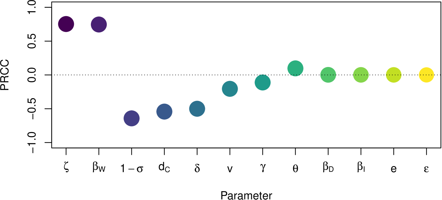
Figure 2: PRCC of $\mathcal{R}_{v}$.

We then proceed to a sensitivity analysis of $\mathcal{R}_{v}$ as a function of models parameters, using a global sensitivity analysis using partial rank correlation coefficients (PRCC). Results are shown in Figure 2. We observe that parameters having the most influence on $\mathcal{R}_{v}$ are the rate at which humans contaminate the water, vaccine effectiveness and the rate of contamination of humans by bacteria. The rate of disease-induced death of course greatly lowers the reproduction number, although this is not a control parameter of the disease. Besides vaccine effectiveness $1-\sigma$, other control parameters playing an important role in lowering $\mathcal{R}_{v}$ are the vaccination rate $v$ and the death rate $d_{C}$ of bacteria. Interestingly, parameters related to the route of transmission through infectious dead individuals ($e$ and $\beta_{D}$) have virtually no effect on the reproduction number $\mathcal{R}_{v}$.

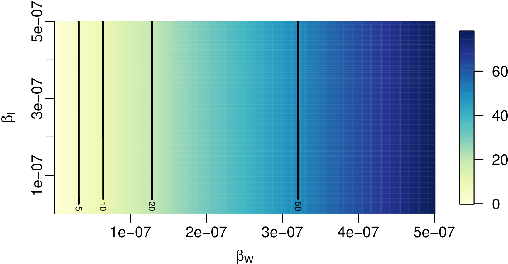
(a) $\beta_{W}$ and $\beta_{I}$

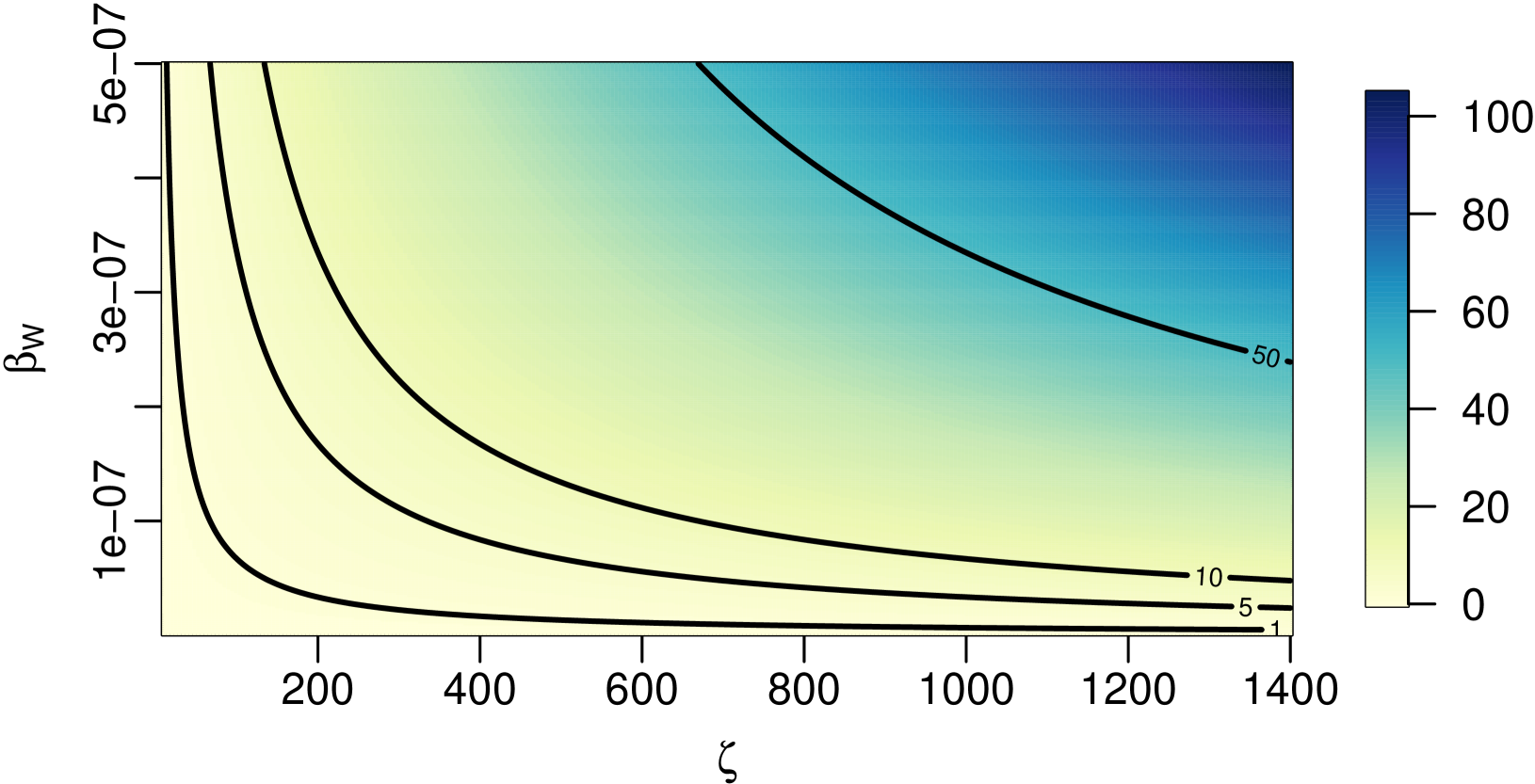
(b) $\zeta$ and $\beta_{W}$

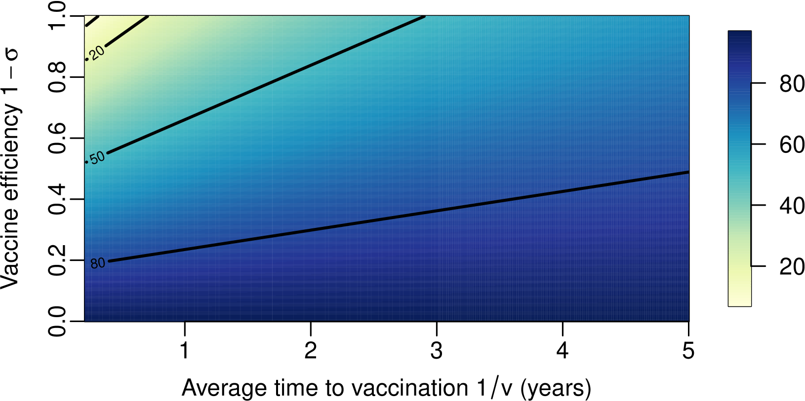
(c) $1/v$ and $1-\sigma$

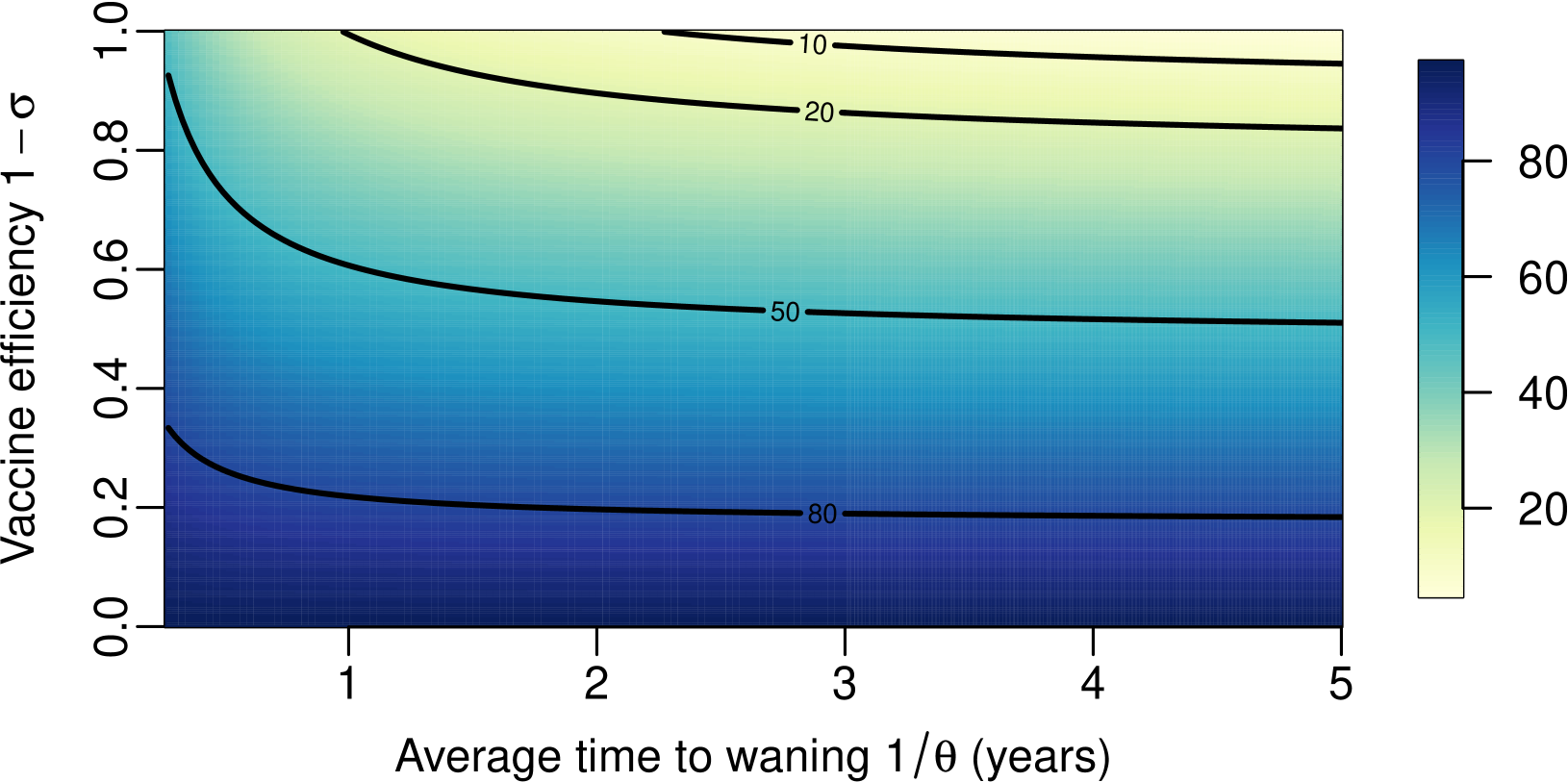
(d) $1/\theta$ and $1-\sigma$

Figure 3: Variation of $\mathcal{R}_{v}$ as a function of (a) water-to-human and human-to-human contamination coefficients, (b) shedding rate of the pathogen by infected humans and water-to-human contamination coefficient, (c) mean time to vaccination and vaccine efficiency and (d) mean time to vaccine waning and vaccine efficiency. Parameters taken as their default values in Table 3 except for those made to vary in a figure.

In the heatmaps of Figure 3, we explore in more detail how different parameters influence the vaccinated reproduction number $\mathcal{R}_{v}$. Note that the values of $\mathcal{R}_{v}$ shown are large but not inconsistent with values found in the literature [13, 43].

First, observe in Figure 3(a) that $\mathcal{R}_{v}$ depends much less on $\beta_{I}$ (human-to-human transmission) than it does on $\beta_{W}$ (water-to-human transmission), where both $\beta_{I}$ and $\beta_{W}$ vary in the same range. The situation is the same when plotting $\mathcal{R}_{v}$ as a function of $\beta_{W}$ and $\beta_{D}$ or, even, $\beta_{I}$ and $\beta_{D}$, although we do not show these plots for lack of space. Because of this observation and that in Figure 2, the remainder of the computational analysis now omits parameters related to transmission originating from infectious dead bodies.

Figure 3(b) then considers the effect of two parameters whose values can be changed by using the WASH strategy: the rate $\zeta$ at which humans contaminate water and the coefficient $\beta_{W}$ of water-to-human pathogen transmission. Here, the effect is similar: decreasing the rate of contamination of water by humans, e.g., by using proper sanitation methods, or that of contaminations of humans by contaminated water, e.g., using hand washing or filtration, have the effect of greatly reducing the vaccinated reproduction number $\mathcal{R}_{v}$.

We now turn to the effect of vaccination. In Figure 3(c), we consider the average time to vaccination in years and the vaccine efficiency. Note that in an epidemic situation, high waiting times for vaccination as shown towards the right of Figure 3(c) are unrealistic, but they may be used in a routine vaccination scenario. The ideal situation here is, unsurprisingly, with low waiting time to vaccination and high vaccine efficiency. The latter is a characteristic of the vaccine and hard to address in the short term, but the former is “easily” accessible through policy. Likewise, Figure 3(d) shows how $\mathcal{R}_{v}$ changes as a function of the mean time $1/\theta$ to loss of vaccine protection and vaccine efficiency $1-\sigma$. We see that vaccine efficiency is the main driver of $\mathcal{R}_{v}$ here, with however a marked turn for the worse when the mean time to waning is small.

Taken together, these results confirm that combined strategies aiming to reduce both direct and environmental transmission while increasing vaccination coverage are crucial for controlling the infection.

To conclude on computational considerations, as mentioned in Section 3, we postulate that Conjecture 3.7 holds, i.e., that the endemic equilibrium points $\bm{E}^{\star}$ and $\bm{E}_{\star}$ are, respectively, locally asymptotically stable and unstable when they are relevant. As we have been so far unable to prove this result analytically, we have considered the problem numerically: in all the numerical simulations in Section 4, equilibria were computed for any value in parameter space used, then we checked which of the situations in Proposition 3.4 held and computed all eigenvalues of the Jacobian matrix of (2.1) at $\bm{E}^{\star}$. As mentioned in Section 4.1, we never observed a situation where $\bm{E}_{\star}$ took a positive value so just checked that whenever $\bm{E}^{\star}$ occured (for $\mathcal{R}_{v}>1$), it was locally asymptotically stable.

5 Discussion

The most important takeaway from (2.1) is that for realistic parameter ranges, sensitivity analyses indicate that contamination from individuals having died from the disease plays very little role in the spread of the infection. This flies in the face of empirical evidence, with for instance [27] finding that during the 1994 cholera epidemic in Guinea-Bissau, eating at a funeral in the presence of non-disinfected corpses as well as washing and transportation of bodies was strongly associated with a rise in cholera cases. However, the cases reported there were at the start of the epidemic, emphasising that it would be useful to extend our present model to focus on the initial phase of the epidemic, e.g., by considering the continuous-time Markov chain associated to (2.1) or its branching process approximation.

Although our analysis shows that a backward bifurcation can take place in (2.1), we were unable find points in parameter space where it would be present: in all the cases we evaluated in Section 4.1, the coefficient $a_{1}$ given by (A.6b) was negative, meaning that since $a_{2}$ is always negative and $a_{0}<0$ when $\mathcal{R}_{v}<1$, there were no subthreshold endemic equilibria. This is not to say that a backward bifurcation can never be observed, since there is no reason a priori that would preclude $a_{1}$ being negative when $\mathcal{R}_{v}<1$, simply that with the somewhat realistic parameters we used, this does not happen. This is reassuring from an epidemiological point of view, as it implies that vaccination has a predictable and favourable effect on disease prevalence.

We finish with a discussion of our assumption that there is no intrinsic V. cholerae population dynamics in the environment. It would definitely be interesting to consider the dynamics of bacteria in the absence of infections in humans and we might do so in the future. However, the models cited with logistic bacteria dynamics are “philosophically equivalent” to our and similar models: bacteria are absent at the disease-free equilibrium and present at the endemic equilibrium(s). We actually expect that a backward bifurcation would still be present in a model with logistic dynamics for the bacteria, although this would have to be confirmed. Indeed, the backward bifurcation arises because vaccination introduces two pathways to infection for “susceptible” individuals (susceptible and vaccinated individuals) who can switch between both pathways because of vaccination and waning. One can intuition that it is the presence within the flow diagram of (2.1) of a subgraph isomorphic to the flow diagram of the SIRVS model in [8, Appendix B] (or possibly even the SIVS model of [33]) that leads to the possibility for a backward bifurcation and that additional compartments $D$ and $W$ in (2.1) do nothing to “break” this.

However, this discussion highlights a more general and fundamental limitation in the analysis of epidemiological models. Indeed, all the cholera models we are aware of (including the present one) assume that V. cholerae are absent at the disease-free equilibrium. While this is a convenient assumption to make in order to facilitate the mathematical analysis, it does not align with biological knowledge, since it “is now well accepted that Vibrio cholerae, the causative agent of the water-borne disease cholera, is acquired from environmental sources where it persists between outbreaks of the disease” [35]. Thus, one should consider models in which there is no disease-free equilibrium for bacteria, implying in turn absence of one for humans and leading to a situation similar in essence to a case with immigration of infectious individuals [5, 10, 16]. This underscores the need for more mathematical work to better understand models without disease-free equilibria.

Acknowledgements

JA is partially supported by the Natural Sciences and Engineering Research Council (NSERC) of Canada through the Discovery Grants program.

Appendix A Proofs

The following lemma is given without proof, as it is quite classic. It is however required in the text.

Lemma A.1.

If initial conditions (2.2) are positive, then solutions of (2.1) are positive for all $t\geq 0$.

With this in mind, we now prove Lemma 3.1.

Proof of Lemma 3.1.

We have

$$N^{\prime}_{H} =S^{\prime}+I^{\prime}+R^{\prime}+V^{\prime}=b-\delta I-d_{H}N_{H}\leq b-d_{H}N_{H},$$ (A.1)

Thus,

$$N_{H}(t)\leq e^{-td_{H}}\left[N_{H}(0)-\frac{b}{d_{H}}\right]+\frac{b}{d_{H}}.$$

Taking the limit, we obtain that for all sufficiently large $t$,

$$N_{H}(t)\leq\frac{b}{d_{H}}.$$

Now

$$W^{\prime} =\zeta I-d_{C}W\leq\zeta\frac{b}{d_{H}}-d_{C}W\implies W(t)\leq\frac{\zeta b}{d_{C}d_{H}}$$

for all sufficiently large $t$. Finally,

$$D^{\prime} =\delta I-eD\leq\delta\frac{b}{d_{H}}-eD$$

and thus, for all sufficiently large $t$,

$$D(t)\leq\frac{\delta b}{ed_{H}}.$$

Clearly, solutions starting in $\Omega$ satisfy these inequalities for all $t\geq 0$, giving also the positive invariance of $\Omega$. ∎

To prove Theorem 3.3, we need the following result, which we prove first.

Lemma A.2.

In (2.1), the population of susceptible and vaccined individuals is bounded above, and for all sufficiently large $t$, satisfies

$$S(t) \leq\dfrac{b}{d_{H}},$$ (A.2)

$$V(t) \leq\dfrac{vb}{(\theta+d_{H})d_{H}}.$$ (A.3)

Proof.

First, note that from (3.1), there holds that, for all sufficiently large $t$,

$$S(t)\leq N_{H}\leq\dfrac{b}{d_{H}}.$$

Equation (2.1d) implies

$$V^{\prime} =vS-\theta V-\lambda_{V}V-d_{H}V$$

$$\leq vS-\theta V-d_{H}V$$

$$\leq\frac{vb}{d_{H}}-(\theta+d_{H})V.$$

Therefore, passing to the limit,

$$V\leq\dfrac{vb}{d_{H}(\theta+d_{H})}.$$

Boundedness follows immediately from the fact that $S$ and $V$ are asymptotically bounded. ∎

We can now prove Theorem 3.3.

Proof of Theorem 3.3.

Let us first prove the local asymptotic stability part, namely, that the disease-free equilibrium (3.2) is locally asymptotically stable if $\mathcal{R}_{v}<1$ and unstable otherwise.

For this, we need to check that hypotheses (A1)–(A5) of [54, Theorem 2] are satisfied. Hypotheses (A1)–(A4) follow from the procedure used to derive $F$ and $V$ in the computation of $\mathcal{R}_{v}$. Therefore, all we need to check is that the system without disease has the disease-free equilibrium (locally) asymptotically stable. In the absence of disease, (2.1) is the linear system,

$$\begin{pmatrix}S^{\prime}\\ R^{\prime}\\ V^{\prime}\end{pmatrix}=\begin{pmatrix}-v-d_{H}&\varepsilon&\theta\\ 0&-\varepsilon-d_{H}&0\\ v&0&-\theta-d_{H}\end{pmatrix}\begin{pmatrix}S\\ R\\ V\end{pmatrix}+\begin{pmatrix}b\\ 0\\ 0\end{pmatrix}.$$

The matrix in this system is strictly diagonally dominant by columns, so it is invertible and there is a unique positive equilibrium, the disease-free equilibrium (3.2). Furthermore, as all diagonal entries are negative, the Gershgorin Theorem [19] implies that all eigenvalues are negative, so the disease-free equilibrium is always (locally) asymptotically stable, verifying that assumption (A5) in [54, Theorem 2] holds. The result follows.

Let us now consider the global asymptotic stability of $\bm{E}_{0}$ when $\mathcal{R}_{0}<1$. To do this, we show that the function

$$L=I+nD+mW,$$

with $n,m>0$, is a Lyapunov function for (2.1). First, note that $L(\bm{E}_{0})=0$ and $L(S,I,R,V,D,W)\geq 0$. Hence $L$ is positive definite. Then,

$$L^{\prime}(S,I,R,V,D,W) =I^{\prime}+nD+mW^{\prime}$$

$$=\left(\beta_{I}+\beta_{D}D+\beta_{W}W\right)S+\sigma\left(\beta_{I}+\beta_{D}D+\beta_{W}W\right)V$$

$$\quad-(\gamma+\delta+d_{H})I+n\left(\delta I-eD\right)+m\left(\zeta I-d_{C}W\right)$$

$$\leq\dfrac{b}{d_{H}}\left(\beta_{I}I+\beta_{D}D+\beta_{W}W\right)+\dfrac{\sigma vb}{d_{H}(\theta+d_{H})}\left(\beta_{I}I+\beta_{D}D+\beta_{W}W\right)$$

$$\quad-(\gamma+\delta+d_{H})I+n\left(\delta I-eD\right)+m\left(\zeta I-d_{C}W\right)$$

$$\leq\left(\dfrac{b}{d_{H}}\beta_{I}+\dfrac{\sigma vb}{d_{H}(\theta+d_{H})}\beta_{I}-(\gamma+\delta+d_{H})+n\delta+\zeta m\right)I$$

$$\quad+\left(\dfrac{b}{d_{H}}\beta_{D}+\dfrac{\sigma vb}{d_{H}(\theta+d_{H})}\beta_{D}-en\right)D$$

$$\quad+\left(\dfrac{b}{d_{H}}\beta_{W}+\dfrac{\sigma vb}{d_{H}(\theta+d_{H})}\beta_{W}-d_{C}m\right)W.$$

We choose, in the following, the constants $m,n$ such that,

$$\dfrac{b}{d_{H}}\beta_{D}+\dfrac{\sigma vb}{d_{H}(\theta+d_{H})}\beta_{D}-en =0$$

$$\dfrac{b}{d_{H}}\beta_{W}+\dfrac{\sigma vb}{d_{H}(\theta+d_{H})}\beta_{W}-d_{C}m =0,$$

i.e.,

$$n =\dfrac{b}{ed_{H}}\beta_{D}+\dfrac{\sigma vb}{ed_{H}(\theta+d_{H})}\beta_{D}$$

$$m =\dfrac{b}{d_{C}d_{H}}\beta_{W}+\dfrac{\sigma vb}{d_{C}d_{H}(\theta+d_{H})}\beta_{W}.$$

So

$$L^{\prime} \leq\Biggl{[}\dfrac{b}{d_{H}}\beta_{I}+\dfrac{\sigma vb}{d_{H}(\theta+d_{H})}\beta_{I}-(\gamma+\delta+d_{H})$$

$$\qquad+\dfrac{\delta b\beta_{D}}{ed_{H}}+\dfrac{\delta\sigma vb\beta_{D}}{ed_{H}(\theta+d_{H})}+\dfrac{\zeta b\beta_{W}}{d_{C}d_{H}}+\dfrac{\zeta\sigma vb\beta_{W}}{d_{C}d_{H}(\theta+d_{H})}\Biggr{]}I$$

$$\leq\left[\dfrac{b}{d_{H}(\theta+d_{H})}\left(\beta_{I}+\dfrac{\delta\beta_{D}}{e}+\dfrac{\zeta\beta_{W}}{d_{C}}\right)\left(\theta+\sigma v+d_{H}\right)-(\gamma+\delta+d_{H})\right]I$$

$$\leq\left[\dfrac{b\left(ed_{C}\beta_{I}+\delta d_{C}\beta_{D}+\zeta e\beta_{W}\right)\left(\theta+\sigma v+d_{H}\right)}{ed_{C}d_{H}}-(\gamma+\delta+d_{H})\right]I$$

$$\leq\dfrac{(\gamma+\delta+d_{H})\left(\theta+\sigma v+d_{H}\right)}{\theta+d_{H}}\left[\mathcal{R}_{0}-\dfrac{\theta+d_{H}}{\theta+\sigma v+d_{H}}\right]I$$

$$=\left(\gamma+\delta+d_{H}\right)\left[\dfrac{\theta+\sigma v+d_{H}}{\theta+d_{H}}\mathcal{R}_{0}-1\right]I.$$

If $\mathcal{R}_{0}<1$, then $(\theta+\sigma v+d_{H})\mathcal{R}_{0}/(\theta+d_{H})<\mathcal{R}_{0}<1$. So if $\mathcal{R}_{0}<1$, then $L^{\prime}(S,I,R,V,D,W)<0$. Thus, $L$ is indeed a strict Lyapunov function for (2) near the disease-free equilibrium $\bm{E}_{0}$. It follows that the DFE $\bm{E}_{0}$ is globally asymptotically stable when $\mathcal{R}_{0}<1$. Combining the two partial results gives Theorem 3.3. ∎

Proof of Proposition 3.4.

After some computations, we find that at a positive equilibrium, components can be written in terms of the equilibrium value of $I$ as

$$S(I) =\dfrac{\left(b+\gamma\varepsilon I/(\varepsilon+d_{H})\right)\left(\theta+\sigma kI+d_{H}\right)}{\left(\theta+\sigma kI+d_{H}\right)(kI+v+d_{H})-\theta v}$$ (A.4a)

$$R(I) =\dfrac{\gamma I}{\varepsilon+d_{H}}$$ (A.4b)

$$V(I) =\dfrac{v(b+\gamma\varepsilon I/(\varepsilon+d_{H}))}{\left(\theta+\sigma kI+d_{H}\right)(kI+v+d_{H})-\theta v}$$ (A.4c)

$$D(I) =\dfrac{\delta I}{e}$$ (A.4d)

$$W(I) =\dfrac{\zeta I}{d_{C}},$$ (A.4e)

where $k={\left(ed_{C}\beta_{I}+d_{C}\delta\beta_{D}+e\beta_{D}\zeta\right)}/({ed_{C}})$. The value of $I$ at an endemic equilibrium is itself the root of the quadratic polynomial

$$P(I)=a_{0}+a_{1}I+a_{2}I^{2},$$ (A.5)

where

$$a_{0} =d_{H}\left(\gamma+\delta+d_{H}\right)\left(\theta+v+d_{H}\right)\left(\mathcal{R}_{v}-1\right),$$ (A.6a)

$$a_{1} =k\left[b\sigma k+\frac{\gamma\varepsilon(\theta+\sigma v+d_{H})}{\varepsilon+d_{H}}-\left(\gamma+\delta+d_{H}\right)\left(\theta+\sigma v+\sigma d_{H}+d_{H}\right)\right]$$ (A.6b)

and

$$a_{2} =-\sigma k^{2}\left[\left(\gamma+\delta+d_{H}\right)-\frac{\varepsilon\gamma}{\varepsilon+d_{H}}\right]<0.$$ (A.6c)

From (A.6a), the sign of $a_{0}$ is that of $\mathcal{R}_{v}-1$.

If $I_{1,2}$ are the roots of $P(I)=0$, then $P(I)=I^{2}-(I_{1}+I_{2})I+I_{1}I_{2}=0$. Denote $s=I_{1}+I_{2}$ and $p=I_{1}I_{2}$. Note that $s=a_{1}/a_{2}$ and $p=a_{0}/a_{2}$.

We have $p<0\iff a_{0}>0$ since $a_{2}<0$. So, if $a_{0}>0$, i.e., from (A.6a), if $\mathcal{R}_{v}>1$, then there is only one positive root, since the product of the roots is negative.

Now suppose that $p>0$. In this case, $a_{0}<0$, i.e., $\mathcal{R}_{v}<1$. If $s>0$, then $a_{1}<0$, i.e., $I_{1}+I_{2}>0$, $I_{1}I_{2}>0$ and the two roots are positive. If $s<0$, then $a_{1}>0$, i.e., $I_{1}+I_{2}<0$ and $I_{1}I_{2}>0$ and the two roots are negative.

Note that this assumes that the discriminant $s^{2}-4p$ is nonnegative. In this case, i.e., $s>0$ and $p>0$, i.e., if $\mathcal{R}_{v}<1$ and $a_{1}>0$, (A.5) has two positive real roots given by $I^{\star}=({s+\sqrt{s^{2}-4p}})/{2}$ and $I_{\star}=({s-\sqrt{s^{2}-4p}})/{2}$, which coalesce when $\mathcal{R}_{v}=\mathcal{R}_{c}$, where $\mathcal{R}_{c}$ is the surface $\mathcal{R}_{c}$ where $s^{2}-4p=0$, i.e., the location in parameter space of the pitchfork bifurcation.

Thus, the conditions stated in the result are obtained.

When the root of (A.5) is unique, it is denoted $I^{\star}$, whereas if there are two distinct positive roots, these values are denoted $I^{\star}$ and $I_{\star}$, with the convention that $I_{\star}<I^{\star}$. The resulting endemic equilibria obtained using (A.4a) are denoted as $\bm{E}^{\star}$ and $\bm{E}_{\star}$. According to the properties of (A.4a), all components of $\bm{E}^{\star}$ are greater than those of $\bm{E}_{\star}$, except for $I^{\star}>I_{\star}$.

Since $S(I^{\star}),R(I^{\star}),V(I^{\star}),D(I^{\star})$ and $W(I^{\star})$ are positive when $I^{\star}$ is positive, the result follows from analysis of $P(I)=0$. ∎

References

- [1] H. Abdul-Satar and R.K. Naji. Stability and bifurcation of a cholera epidemic model with saturated recovery rate. Applications & Applied Mathematics, 16(2), 2021.
- [2] S.A. Adefisan. A mathematical model of Ebola Virus Disease. Master’s thesis, University of Manitoba, 2018.
- [3] M. Al-Arydah, A. Mwasa, J.M. Tchuenche, and R.J. Smith? Modeling cholera disease with education and chlorination. Journal of Biological Systems, 21(04):1340007, 2013.
- [4] S. Almagro-Moreno and R.K. Taylor. Cholera: environmental reservoirs and impact on disease transmission. Microbiology Spectrum, 1(2):10–1128, 2013.
- [5] R.M. Almarashi and C.C. McCluskey. The effect of immigration of infectives on disease-free equilibria. Journal of Mathematical Biology, 79:1015–1028, 2019.
- [6] J. Arino, K.L. Cooke, P. van den Driessche, and J. Velasco-Hernández. An epidemiology model that includes a leaky vaccine with a general waning function. DCDS-B, 4(2):479–495, 2004.
- [7] J. Arino, C.C. McCluskey, and P. van den Driessche. Global results for an epidemic model with vaccination that exhibits backward bifurcation. SIAM Journal on Applied Mathematics, 64(1):260–276, 2003.
- [8] J. Arino and E. Milliken. Bistability in deterministic and stochastic SLIAR-type models with imperfect and waning vaccine protection. Journal of Mathematical Biology, 84(7):61, 2022.
- [9] D. Bernoulli. Essai d’une nouvelle analyse de la mortalité causée par la petite vérole et des avantages de l’inoculation pour la prévenir. Histoire de l’Académie Royale des Sciences, Paris, avec les Mémoires de Mathématique et de Physique, pages 1–45, 1766. This paper was presented in 1760 and published in 1766 in the volume for the year 1760.
- [10] F. Brauer and P. van den Driessche. Models for transmission of disease with immigration of infectives. Mathematical Biosciences, 171(2):143–154, 2001.
- [11] V. Capasso and S.L. Paveri-Fontana. A mathematical model for the 1973 cholera epidemic in the European Mediterranean region. Revue d’épidémiologie et de santé publique, 27(2):121–132, 1979.
- [12] T.A.O. Cardoso and D.N. Vieira. Study of mortality from infectious diseases in Brazil from 2005 to 2010: risks involved in handling corpses. Ciência & Saúde Coletiva, 21:485–496, 2016.
- [13] C.H. Chan, A.R. Tuite, and D.N. Fisman. Historical epidemiology of the second cholera pandemic: relevance to present day disease dynamics. PloS one, 8(8):e72498, 2013.
- [14] C.T. Codeço. Endemic and epidemic dynamics of cholera: the role of the aquatic reservoir. BMC Infectious Diseases, 1:1–14, 2001.
- [15] J.M. Conly and B.L. Johnston. Natural disasters, corpses and the risk of infectious diseases. The Canadian Journal of Infectious Diseases & Medical Microbiology, 16(5):269, 2005.
- [16] C. Djuikem and J. Arino. Transmission of multiple pathogens across species. arXiv preprint arXiv:2405.20264, 2024.
- [17] J. Dushoff, W. Huang, and C. Castillo-Chavez. Backwards bifurcations and catastrophe in simple models of fatal diseases. Journal of Mathematical Biology, 36:227–248, 1998.
- [18] F. Federspiel and M. Ali. The cholera outbreak in Yemen: lessons learned and way forward. BMC Public Health, 18(1):1338, 2018.
- [19] D.G. Feingold and R.S. Varga. Block diagonally dominant matrices and generalizations of the Gerschgorin circle theorem. Pacific Journal of Mathematics, 12(4):1241–1250, 1962.
- [20] R.A. Finkelstein. Cholera, Vibrio cholerae o1 and o139, and other pathogenic vibrios. In S. Baron, editor, Medical Microbiology. University of Texas Medical Branch at Galveston, 4th edition, 1996.
- [21] D. Ganesan, S.S. Gupta, and D. Legros. Cholera surveillance and estimation of burden of cholera. Vaccine, 38:A13–A17, 2020.
- [22] R. Ganguly, L.W. Clem, Z. Benčić, R. Sinha, R. Sakazaki, and R.H. Waldman. Antibody response in the intestinal secretions of volunteers immunized with various cholera vaccines. Bulletin of the World Health Organization, 52(3):323, 1975.
- [23] U. Ghosh-Dastidar and S. Lenhart. Modeling the effect of vaccines on cholera transmission. Journal of Biological Systems, 23(02):323–338, 2015.
- [24] Government of Canada. For health professionals: Cholera, 2018. Accessed February 26, 2025.
- [25] D. Greenhalgh, M. Doyle, and F. Lewis. A mathematical treatment of AIDS and condom use. Mathematical Medicine and Biology, 18(3):225–262, 2001.
- [26] A.B. Gumel. Causes of backward bifurcations in some epidemiological models. Journal of Mathematical Analysis and Applications, 395(1):355–365, 2012.
- [27] G. Gunnlaugsson, J. Einarsdottir, F.J. Angulo, S.A. Mentambanar, A. Passa, and R.V. Tauxe. Funerals during the 1994 cholera epidemic in Guinea-Bissau, West Africa: the need for disinfection of bodies of persons dying of cholera. Epidemiology & Infection, 120(1):7–15, 1998.
- [28] K.P. Hadeler and P. van den Driessche. Backward bifurcation in epidemic control. Mathematical Biosciences, 146(1):15–35, 1997.
- [29] N. Hirsch, E. Kappe, A. Gangl, K. Schwartz, A. Mayer-Scholl, J. Hammerl, and E. Strauch. Phenotypic and genotypic properties of vibrio cholerae non-o1, non-o139 isolates recovered from domestic ducks in Germany. Microorganisms, 8(8):1104, 2020.
- [30] W. Huang, K. L. Cooke, and C. Castillo-Chavez. Stability and bifurcation for a multiple-group model for the dynamics of HIV/AIDS transmission. SIAM Journal on Applied Mathematics, 52(3):835–854, 1992.
- [31] J. Jacquez and C. Simon. Qualitative theory of compartmental systems. SIAM Review, 35(1):43–79, 1993.
- [32] R.I. Joh, H. Wang, H. Weiss, and J.S. Weitz. Dynamics of indirectly transmitted infectious diseases with immunological threshold. Bulletin of Mathematical Biology, 71:845–862, 2009.
- [33] C. Kribs-Zaleta and J. Velasco-Hernández. A simple vaccination model with multiple endemic states. Mathematical Biosciences, 164:183–201, 2000.
- [34] T. Leung, J. Eaton, and L. Matrajt. Optimizing one-dose and two-dose cholera vaccine allocation in outbreak settings: A modeling study. PLOS Neglected Tropical Diseases, 16(4):e0010358, 2022.
- [35] C. Lutz, M. Erken, P. Noorian, S. Sun, and D. McDougald. Environmental reservoirs and mechanisms of persistence of Vibrio cholerae. Frontiers in Microbiology, 4:375, 2013.
- [36] R. Milwid, A. Steriu, J. Arino, J. Heffernan, A. Hyder, D. Schanzer, E. Gardner, M. Haworth-Brockman, H. Isfeld-Kiely, J.M. Langley, and S.M. Moghadas. Toward standardizing a lexicon of infectious disease modeling terms. Frontiers in Public Health, 4:213, 2016.
- [37] O. Morgan. Infectious disease risks from dead bodies following natural disasters. Revista Panamericana de Salud Pública, 15:307–312, 2004.
- [38] B.A. Muzembo, K. Kitahara, A. Debnath, A Ohno, K. Okamoto, and S.-I. Miyoshi. Cholera outbreaks in India, 2011–2020: a systematic review. International Journal of Environmental Research and Public Health, 19(9):5738, 2022.
- [39] C.H. Nkwayep, R.G. Kakaï, and S. Bowong. Prediction and control of cholera outbreak: Study case of Cameroon. Infectious Disease Modelling, 9(3):892–925, 2024.
- [40] M.O. Onuorah, F.A. Atiku, and H. Juuko. Mathematical model for prevention and control of cholera transmission in a variable population. Research in Mathematics, 9(1):2018779, 2022.
- [41] M. Pascual, M.J. Bouma, and A.P. Dobson. Cholera and climate: revisiting the quantitative evidence. Microbes and Infection, 4(2):237–245, 2002.
- [42] Pasteur Institute. Cholera: Symptoms, treatment, prevention, 2024. Accessed February 26, 2025.
- [43] M. Phelps, M.L. Perner, V.E. Pitzer, V. Andreasen, P.K.M. Jensen, and L. Simonsen. Cholera epidemics of the past offer new insights into an old enemy. The Journal of Infectious Diseases, 217(4):641–649, 2018.
- [44] J. Piret and G. Boivin. Pandemics throughout history. Frontiers in Microbiology, 11:631736, 2021.
- [45] D. Sharma and V. Kumari. Backward bifurcation in a cholera model with a general treatment function. Journal of Biological Systems, 25(1):21–45, 2017.
- [46] S. Sharma and N. Kumari. Backward bifurcation in a cholera model: A case study of outbreak in Zimbabwe and Haiti. International Journal of Bifurcation and Chaos, 27(11):1750170, 2021.
- [47] S. Sharma and F. Singh. Backward bifurcation in a cholera model with a general treatment function. SN Applied Sciences, 3:1–8, 2021.
- [48] S. Sharma and F. Singh. Bifurcation and stability analysis of a cholera model with vaccination and saturated treatment. Chaos, Solitons & Fractals, 146:110912, 2021.
- [49] G. Sun, J.-H. Xie, S.-H. Huang, Z. Jin, M.-T. Li, and L. Liu. Transmission dynamics of cholera: Mathematical modeling and control strategies. Communications in Nonlinear Science and Numerical Simulation, 45:235–244, 2017.
- [50] A.J.O. Tassé, B. Tsanou, J.-L. Woukeng, and J.M.S. Lubuma. A metapopulation model with exit screening measure for the 2014–2016 West Africa Ebola virus outbreak. Mathematical Biosciences, 378:109321, 2024.
- [51] D.L. Taylor, T.M. Kahawita, S. Cairncross, and J.H.J. Ensink. The impact of water, sanitation and hygiene interventions to control cholera: a systematic review. PLoS OBE, 10(8):e0135676, 2015.
- [52] J.H. Tien and D.J.D. Earn. Multiple transmission pathways and disease dynamics in a waterborne pathogen model. Bulletin of Mathematical Biology, 72:1506–1533, 2010.
- [53] A.R. Tuite, J. Tien, M. Eisenberg, D.J.D. Earn, J. Ma, and D.N. Fisman. Cholera epidemic in Haiti, 2010: using a transmission model to explain spatial spread of disease and identify optimal control interventions. Annals of Internal Medicine, 154(9):593–601, 2011.
- [54] P. van den Driessche and J. Watmough. Reproduction numbers and sub-threshold endemic equilibria for compartmental models of disease transmission. Mathematical Biosciences, 180:29–48, 2002.
- [55] J. Wang. Mathematical models for cholera dynamics—a review. Microorganisms, 10(12), 2022.
- [56] World Health Organization. Cholera vaccines: WHO position paper. Weekly Epidemiological Record, 85(13):117–128, 2010.
- [57] World Health Organization. Cholera vaccines: WHO position paper–August 2017. Weekly Epidemiological Record, 92(34):477–498, 2017.
- [58] World Health Organization. Cholera, 2024. https://www.who.int/news-room/fact-sheets/detail/cholera – Accessed February 26, 2025.
- [59] X. Zhou and J. Cui. Modeling and stability analysis for a cholera model with vaccination. Mathematical Methods in the Applied Sciences, 34(14):1711–1724, 2011.