A Unified Framework and Efficient Computation for Privacy Amplification via Shuffling

Abstract.

The shuffle model offers significant privacy amplification over local differential privacy (LDP), enabling improved privacy-utility trade-offs. To analyze and quantify this amplification effect, two primary frameworks have been proposed: the privacy blanket (Balle et al., CRYPTO 2019) and the clone paradigm, which includes both the standard clone and stronger clone (Feldman et al., FOCS 2021; SODA 2023). All of these approaches are grounded in decomposing the behavior of local randomizers.

In this work, we present a unified perspective—termed the general clone paradigm—that captures all decomposition-based analyses. We identify the optimal decomposition within this framework and design a simple yet efficient algorithm based on the Fast Fourier Transform (FFT) to compute tight privacy amplification bounds. Empirical results show that our computed upper bounds nearly match the corresponding lower bounds, demonstrating the accuracy and tightness of our method.

Furthermore, we apply our algorithm to derive optimal privacy amplification bounds for both joint composition and parallel composition of LDP mechanisms in the shuffle model.

1. Introduction

Differential Privacy (DP) has become a foundational framework for safeguarding individual privacy while enabling meaningful data analysis (Dwork, 2006). In real-world applications, Local Differential Privacy (LDP) is widely adopted as it eliminates the need for a trusted curator by applying noise to each user’s data before aggregation (Cormode et al., 2018a; Ding et al., 2017; Yang et al., 2024a; Team, 2017). However, this decentralized approach often results in significant utility loss due to excessive noise.

To address this trade-off, the shuffle model introduces a trusted shuffler between users and the aggregator (Cheu et al., 2019; Erlingsson et al., 2019; Bittau et al., 2017). The shuffler permutes the locally perturbed data, breaking the link between individual users and their submitted values. Shuffle DP retains the trust-free nature of LDP while significantly improving the privacy-utility trade-off, making it a promising model for real-world deployment (Wang et al., 2020; Imola et al., 2022; Cheu and Zhilyaev, 2022). For instance, privacy amplification by shuffling was used in Apple and Google’s Exposure Notification Privacy-preserving Analytics (Apple and Google, 2021).

The amplification effect in the shuffle model implies that when each of the $n$ users randomizes their data using an $\epsilon_{0}$-LDP mechanism, the collection of shuffled reports satisfies $(\epsilon(\epsilon_{0},\delta,n),\delta)$-DP, where $\epsilon(\epsilon_{0},\delta,n)\ll\epsilon_{0}$ for sufficiently large $n$ and $1/\delta$ (Feldman et al., 2023a). A central theoretical challenge is to characterize and compute this privacy amplification effect. A tighter bound allows for a larger value of $\epsilon_{0}$ while still achieving $(\epsilon,\delta)$-DP after shuffling, thereby improving the utility of the mechanism. It also enables a more accurate analysis of the overall $(\epsilon,\delta)$-guarantees resulting from shuffling $n$ independent $\epsilon_{0}$-LDP reports.

Researchers are interested in two types of upper bounds on privacy amplification. The first is a generic bound, which provides a uniform guarantee for all $\epsilon_{0}$-DP local randomizers. The second is a specific bound, which is tailored for a given $\epsilon_{0}$-DP local randomizer. Generic bounds are primarily studied from a theoretical perspective, as they allow the derivation of asymptotic expressions for $\epsilon(\epsilon_{0},n,\delta)$ (Balle et al., 2019; Feldman et al., 2022). In contrast, specific bounds are usually much tighter and are of significant practical importance, as they provide precise guarantees for concrete mechanisms used in real-world applications.

Among the various strategies proposed to analyze this effect (Cheu et al., 2019; Erlingsson et al., 2019; Balle et al., 2020), decomposition-based approaches have demonstrated the strongest performance (Balle et al., 2019; Feldman et al., 2022, 2023a). Two prominent frameworks are the privacy blanket by Balle et al. (Balle et al., 2019) and the clone paradigm by Feldman et al. (Feldman et al., 2022, 2023a), which includes the standard clone and the stronger clone. These approaches rely on decomposing the probability distributions induced by a local randomizer under different inputs. A decomposition naturally leads to a reduction, which yields an upper bound on the privacy amplification achieved by shuffling.

The privacy blanket framework designs a tailored decomposition to obtain a bound for each specific local randomizer. However, this bound cannot be computed precisely in its original form. To address this, the framework resorts to further approximations—such as Hoeffding’s and Bennett’s inequalities—which yield looser but computable bounds. A computable generic bound is also derived in a similar manner.

The standard clone paradigm (Feldman et al., 2022) adopts a simple, unified decomposition, resulting in a generic bound that applies to all $\epsilon_{0}$-DP local randomizers. This bound can be computed precisely using a dedicated numerical algorithm and empirically outperforms the computable generic bound derived from the privacy blanket framework. However, the standard clone does not provide any specific bounds.

The stronger clone (Feldman et al., 2023a) was introduced with a more refined decomposition and was expected to yield improved bounds for both generic and specific local randomizers. Unfortunately, a critical flaw was later identified in the proof’s core lemma. A corrected version was released on arXiv (Feldman et al., 2023b), which showed that the original generic bounds hold only for a restricted class of local randomizers. The specific bounds were also revised and replaced with a version that is much weaker and lacks an efficient computation method.

Our focus: specific bounds.

In this paper, we focus on computing specific bounds. We provide the optimal bound achievable via any decomposition-based method for a given randomizer. Furthermore, we introduce an efficient numerical algorithm that can compute this optimal bound precisely.

To identify the optimal bound, we propose a unified analysis framework—the general clone paradigm-which encompasses all possible decompositions, and further show the best decomposition is the one used by the privacy blanket. However, the decomposition bound of the privacy blanket in its original form cannot be directly computed. Fortunately, we represent the decomposition bound in a simple form and propose a numerical algorithm using Fast Fourier Transform (FFT) to efficiently compute the bound.

With these results, we achieve the best-known bounds obtainable through decomposition-based methods. Experimental results show that our computed upper bounds closely match the empirical lower bounds, demonstrating the tightness and reliability of our analysis. Notably, our new bounds yield at least a 10% improvement in the value of $\epsilon$ across all settings, and the improvement can reach up to 50% when $\epsilon_{0}$ is large and $n$ is small.

Additionally, we discuss a potential direction to move beyond decomposition methods: identifying the exact amplification without bounding. While this approach is intuitively appealing, it currently lacks the necessary theoretical tools and remains an open problem.

Finally, we conduct the first systematic analysis of joint composition in the shuffle model using our algorithm. In classical DP, $k$-fold composition refers to applying $k$ independent mechanisms to the same dataset:

$$\mathcal{M}_{kFold}(D)=(\mathcal{M}_{1}(D),\mathcal{M}_{2}(D),\dots,\mathcal{M}_{k}(D)).$$

In contrast, our notion of joint composition applies independent mechanisms to different datasets:

$$\mathcal{M}_{joint}(D_{1},D_{2},\dots,D_{k})=(\mathcal{M}_{1}(D_{1}),\mathcal{M}_{2}(D_{2}),\dots,\mathcal{M}_{k}(D_{k})).$$

Joint composition is widely used in LDP applications such as joint distribution estimation and heavy hitter detection (Domingo-Ferrer and Soria-Comas, 2022; Ren et al., 2018; Bassily and Smith, 2015; Kikuchi, 2022). For example, when each user’s data contains $d$ attributes, applying an $\frac{\epsilon_{0}}{d}$-LDP mechanism to each attribute ensures overall $\epsilon_{0}$-LDP while preserving inter-attribute correlations.

While existing studies have analyzed $k$-fold composition in the shuffle model (Koskela et al., 2021, 2020), we focus on the case where the local mechanism itself is a joint composition. Our experimental results show that existing methods yield relatively loose bounds in this setting, whereas our algorithm computes significantly tighter results by leveraging the optimal bounds.

Additionally, we show how to compute the optimal bounds for the parallel composition of LDP protocols. This setting was previously studied in (Wang et al., 2024), but their analysis inherited a technical flaw from (Feldman et al., 2023a), resulting in incorrect conclusions. Our method corrects this and provides the first correct computation of the optimal bound in this setting.

Our contributions can be summarized as follows:

• We propose the general clone paradigm, which subsumes all decomposition-based methods, and identify the optimal bound it can provide for a specific local randomizer.

• We provide an efficient numerical algorithm for computing the optimal bounds via FFT.

• We present methods for computing optimal amplification bounds for both joint composition and parallel composition in the shuffle model, achieving substantially tighter results than existing approaches.

2. Preliminaries

Differential privacy is a privacy-preserving framework for randomized algorithms. Intuitively, an algorithm is differentially private if the output distribution does not change significantly when a single individual’s data is modified. This ensures that the output does not reveal substantial information about any individual in the dataset. The hockey-stick divergence is commonly used to define $(\epsilon,\delta)$-DP.

Definition 0 (Hockey-Stick Divergence).

The hockey-stick divergence between two random variables $P$ and $Q$ is defined as:

$$D_{\alpha}(P\parallel Q)=\int\max\{0,P(x)-\alpha Q(x)\}\,\mathrm{d}x,$$

where we use the notation $P$ and $Q$ to refer to both the random variables and their probability density functions.

We say that $P$ and $Q$ are $(\epsilon,\delta)$-indistinguishable if:

$$\max\{D_{e^{\epsilon}}(P\parallel Q),D_{e^{\epsilon}}(Q\parallel P)\}\leq\delta.$$

If two datasets $X^{0}$ and $X^{1}$ have the same size and differ only by the data of a single individual, they are referred to as neighboring datasets (denoted by $X^{0}\simeq X^{1}$).

Definition 0 (Differential Privacy).

An algorithm $\mathcal{R}:\mathbb{X}^{n}\to\mathbb{Z}$ satisfies $(\epsilon,\delta)$-differential privacy if for all neighboring datasets $X,X^{\prime}\in\mathbb{X}^{n}$, $\mathcal{R}(X)$ and $\mathcal{R}(X^{\prime})$ are $(\epsilon,\delta)$-indistinguishable.

Definition 0 (Local Differential Privacy).

An algorithm $\mathcal{R}:\mathbb{X}\to\mathbb{Y}$ satisfies local $(\epsilon,\delta)$-differential privacy if for all $x,x^{\prime}\in\mathbb{X}$, $\mathcal{R}(x)$ and $\mathcal{R}(x^{\prime})$ are $(\epsilon,\delta)$-indistinguishable.

Here, $\epsilon$ is referred to as the privacy budget, which controls the privacy loss, while $\delta$ allows for a small probability of failure. When $\delta=0$, the mechanism is also called $\epsilon$-DP.

Following conventions in the shuffle model based on randomize-then-shuffle (Balle et al., 2019; Cheu et al., 2019), we define a single-message protocol $\mathcal{P}$ in the shuffle model as a pair of algorithms $\mathcal{P}=(\mathcal{R},\mathcal{A})$, where $\mathcal{R}:\mathbb{X}\to\mathbb{Y}$, and $\mathcal{A}:\mathbb{Y}^{n}\to\mathbb{O}$. We call $\mathcal{R}$ the local randomizer, $\mathbb{Y}$ the message space of the protocol, $\mathcal{A}$ the analyzer, and $\mathbb{O}$ the output space.

The overall protocol implements a mechanism $\mathcal{P}:\mathbb{X}^{n}\to\mathbb{O}$ as follows: Each user $i$ holds a data record $x_{i}$, to which they apply the local randomizer to obtain a message $y_{i}=\mathcal{R}(x_{i})$. The messages $y_{i}$ are then shuffled and submitted to the analyzer. Let $\mathcal{S}(y_{1},\dots,y_{n})$ denote the random shuffling step, where $\mathcal{S}:\mathbb{Y}^{n}\to\mathbb{Y}^{n}$ is a shuffler that applies a random permutation to its inputs.

In summary, the output of $\mathcal{P}(x_{1},\dots,x_{n})$ is given by

$$\mathcal{A}\circ\mathcal{S}\circ\mathcal{R}^{n}(\boldsymbol{x})=\mathcal{A}(\mathcal{S}(\mathcal{R}(x_{1}),\dots,\mathcal{R}(x_{n}))).$$

Definition 0 (Differential Privacy in the Shuffle Model).

A protocol $\mathcal{P}=(\mathcal{R},\mathcal{A})$ satisfies $(\epsilon,\delta)$-differential privacy in the shuffle model if for all neighboring datasets $X,X^{\prime}\in\mathbb{X}^{n}$, the distributions $\mathcal{S}\circ\mathcal{R}^{n}(X)$ and $\mathcal{S}\circ\mathcal{R}^{n}(X^{\prime})$ are $(\epsilon,\delta)$-indistinguishable.

3. Review of Existing Analysis Techniques

In this section, we review existing analysis techniques for studying privacy amplification in the shuffle model. We begin by introducing the standard clone paradigm due to its simplicity (Feldman et al., 2022). Next, we restate the privacy blanket framework, using consistent terminology with the former (Balle et al., 2019). On one hand, this clarifies misconceptions about the privacy blanket framework found in subsequent literature (Koskela et al., 2021). On the other hand, it aids in identifying the intrinsic connection between the two approaches, which will be explored in Section 4.

We then discuss the subsequent attempts to extend the clone paradigm, specifically the stronger clone. We show the vision and failure of both the original and corrected versions of the stronger clone.

3.1. Standard clone

The intuition behind the standard clone paradigm is as follows (Feldman et al., 2022): Suppose that $X^{0}$ and $X^{1}$ are neighbouring databases that differ on the first datapoint, $x_{1}^{0}\neq x_{1}^{1}$. A key observation is that for any $\varepsilon_{0}$-DP local randomizer $\mathcal{R}$ and data point $x$, $\mathcal{R}(x)$ can be seen as sampling from the same distribution as $\mathcal{R}(x_{1}^{0})$ with probability at least $e^{-\varepsilon_{0}}/2$ and sampling from the same distribution as $\mathcal{R}(x_{1}^{1})$ with probability at least $e^{-\varepsilon_{0}}/2$. That is, with probability $e^{-\varepsilon_{0}}$ each data point can create a clone of the output of $\mathcal{R}(x_{1}^{0})$ or a clone of $\mathcal{R}(x_{1}^{1})$ with equal probability. Thus $n-1$ data elements effectively produce a random number of clones of both $x_{1}^{0}$ and $x_{1}^{1}$, making it more challenging to distinguish whether the original dataset contains $x_{1}^{0}$ or $x_{1}^{1}$ as its first element.

Due to the $\epsilon_{0}$-DP property of the local randomizer $\mathcal{R}$, we have the following inequality:

$$\forall x_{i}\in\mathbb{X},\forall y\in\mathbb{Y}:\Pr[\mathcal{R}(x_{i})=y]\geq\frac{1}{e^{\epsilon_{0}}}\Pr[\mathcal{R}(x_{1}^{0})=y]$$

$$\wedge\Pr[\mathcal{R}(x_{i})=y]\geq\frac{1}{e^{\epsilon_{0}}}\Pr[\mathcal{R}(x_{1}^{1})=y].$$

Therefore, the local randomizer $\mathcal{R}$ on any input $x_{i}$ can be decomposed into a mixture of $\mathcal{R}(x_{1}^{0}),\mathcal{R}(x_{1}^{1})$ and some “left-over” distribution $\text{LO}(x_{i})$ such that

$$\mathcal{R}(x_{i})=\frac{1}{2e^{\epsilon_{0}}}\mathcal{R}(x_{1}^{0})+\frac{1}{2e^{\epsilon_{0}}}\mathcal{R}(x_{1}^{1})+(1-\frac{1}{e^{\epsilon_{0}}})\text{LO}(x_{i}).$$

Let $\mathcal{M}_{S}=\mathcal{S}\circ\mathcal{R}^{n}$ denote the shuffling of $\mathcal{R}$. To compute the privacy amplification provided by the shuffle model, we need to compute $D_{e^{\epsilon}}(\mathcal{M}_{S}(X^{0}),\mathcal{M}_{S}(X^{1}))$ for a given $\epsilon$. The exact computation is computationally complex, so the researchers seek an upper bound for it. A key property is that hockey-stick divergence satisfies the data processing inequality.

Property 1 (Data Processing Inequality).

For all distributions $P$ and $Q$ defined on a set $S$ and (possibly randomized) functions $f:S\to S^{\prime}$,

$$D_{\alpha}\big{(}f(P)||f(Q)\big{)}\leq D_{\alpha}(P||Q).$$

If we can find two probability distributions $P_{0}$ and $P_{1}$ along with a post-processing function $f$ such that $f(P_{0})=\mathcal{M}_{S}(X^{0})$ and $f(P_{1})=\mathcal{M}_{S}(X^{1})$, then it follows that $D_{e^{\epsilon}}(P_{0},P_{1})$ is an upper bound for $D_{e^{\epsilon}}(\mathcal{M}_{S}(X^{0}),\mathcal{M}_{S}(X^{1}))$. We refer to $(P_{0},P_{1})$ as a reduction pair. Different analysis techniques construct different reduction pairs. We first present an intuitive construction of the reduction pair within the standard clone framework, followed by the formal construction.

Definition 0 (Standard Clone Reduction Pair (Intuitive) (Feldman et al., 2022)).

Define random variables $A_{0},A_{1}$ and $A_{2}$ as follows:

$$A_{0}=\begin{cases}0&\text{w.p. }1\\ 1&\text{w.p. }0\\ 2&\text{w.p. }0\end{cases},\ A_{1}=\begin{cases}0&\text{w.p. }0\\ 1&\text{w.p. }1\\ 2&\text{w.p. }0\end{cases},\text{ and }A_{2}=\begin{cases}0&\text{w.p. }\frac{1}{2e^{\epsilon_{0}}}\\ 1&\text{w.p. }\frac{1}{2e^{\epsilon_{0}}}\\ 2&\text{w.p. }1-\frac{1}{e^{\epsilon_{0}}}\end{cases}$$

To obtain a sample from $P_{0}$ (or $P_{1}$), sample one copy from $A_{0}$ (or $A_{1}$) and $n-1$ copies of $A_{2}$, the output $(n_{0},n_{1})$ where $n_{0}$ is the total number of 0s and $n_{1}$ is the total number of 1s. Equivalently,

$$C\sim\text{Bin}(n-1,\frac{1}{e^{\epsilon_{0}}}),\ A\sim\text{Bin}(C,\frac{1}{2}).$$

$$P_{0}=(A+1,C-A),\ P_{1}=(A,C-A+1).$$

The corresponding post-processing function $f_{1}$ is shown in the Algorithm 1.

Algorithm 1 Post-processing function of standard clone (Feldman et al., 2022), $f_{1}$

$x_{1}^{0},x_{1}^{1},x_{2},\dots,x_{n}$; $y\in\{0,1,2\}^{n}$

$J\leftarrow\emptyset$

for $i=1,\dots,n$ do

  if $y_{i}=2$ then

   Let $j$ be a randomly and uniformly chosen element of $[2:n]\setminus J$

   $J\leftarrow J\cup\{j\}$

  end if

  Sample $z_{i}$ from

   $\begin{cases}\mathcal{R}(x_{1}^{0})&\text{if }y_{i}=0;\\ \mathcal{R}(x_{1}^{1})&\text{if }y_{i}=1;\\ \text{LO}(x_{j})&\text{if }y_{i}=2.\end{cases}$

end for

return $z_{1},\dots,z_{n}$

An additional observation is that if $\mathcal{R}$ is $\epsilon_{0}$-DP, then $\mathcal{R}(x_{1}^{0})$ and $\mathcal{R}(x_{1}^{1})$ are similar, hence privacy is further amplified (Feldman et al., 2022). The similarity is characterized by the following lemma:

Lemma 2 ((Kairouz et al., 2017)).

Let $\mathcal{R}:\mathbb{X}\to\mathbb{Y}$ be an $\epsilon_{0}$-DP local randomizer and $x_{0},x_{1}\in\mathbb{X}$. Then there exists two probability distributions $\mathcal{Q}_{0},\mathcal{Q}_{1}$ such that

$$\mathcal{R}(x_{0})=\frac{e^{\epsilon_{0}}}{e^{\epsilon_{0}}+1}\mathcal{Q}_{0}+\frac{1}{e^{\epsilon_{0}}+1}\mathcal{Q}_{1}$$

and

$$\mathcal{R}(x_{1})=\frac{1}{e^{\epsilon_{0}}+1}\mathcal{Q}_{0}+\frac{e^{\epsilon_{0}}}{e^{\epsilon_{0}}+1}\mathcal{Q}_{1}.$$

With the help of Lemma 2, (Feldman et al., 2022) gives the following decomposition for generic local randomizers:

$$\mathcal{R}(x_{1}^{0}) =\frac{e^{\epsilon_{0}}}{e^{\epsilon_{0}}+1}\mathcal{Q}_{1}^{0}+\frac{1}{e^{\epsilon_{0}}+1}\mathcal{Q}_{1}^{1},$$

$$\mathcal{R}(x_{1}^{1}) =\frac{1}{e^{\epsilon_{0}}+1}\mathcal{Q}_{1}^{0}+\frac{e^{\epsilon_{0}}}{e^{\epsilon_{0}}+1}\mathcal{Q}_{1}^{1},$$

$$\forall i\in[2,n]:\mathcal{R}(x_{i}) =\frac{1}{2e^{\epsilon_{0}}}\mathcal{Q}_{1}^{0}+\frac{1}{2e^{\epsilon_{0}}}\mathcal{Q}_{1}^{1}+(1-\frac{1}{e^{\epsilon_{0}}})\text{LO}(x_{i}).$$

This decomposition leads to the formal reduction of the standard clone:

Theorem 3 (Standard Clone Reduction (Feldman et al., 2022)).

Let $\mathcal{R}:\mathbb{X}\to\mathbb{Y}$ be a $\epsilon_{0}$-DP local randomizer and let $\mathcal{M}_{S}=\mathcal{S}\circ\mathcal{R}^{n}$ be the shuffling of $\mathcal{R}$. For $\varepsilon\geq 0$ and inputs $X^{0}\simeq X^{1}$ with $x_{1}^{0}\neq x_{1}^{1}$, we have

$$D_{e^{\epsilon}}\big{(}\mathcal{M}_{S}(X^{0}),\mathcal{M}_{S}(X^{1})\big{)}\leq D_{e^{\epsilon}}\big{(}P_{0}^{C},P_{1}^{C}\big{)}$$

where $P_{0}^{C},\ P_{1}^{C}$ are defined as below (with “C” denoting “standard Clone”) :

$$C\sim\text{Bin}(n-1,\frac{1}{e^{\epsilon_{0}}}),\quad A\sim\text{Bin}(C,\frac{1}{2}),\quad\text{and }\quad\Delta\sim\text{Bern}(\frac{e^{\epsilon_{0}}}{e^{\epsilon_{0}}+1}).$$

$$P_{0}^{C}=(A+\Delta,C-A+1-\Delta),\quad P_{1}^{C}=(A+1-\Delta,C-A+\Delta).$$

Bern($p$) represents a Bernoulli random variable with bias $p$.

Proof.

We can construct a post-processing function from $(P_{0}^{C},P_{1}^{C})$ to $\big{(}\mathcal{M}_{S}(X^{0}),\mathcal{M}_{S}(X^{1})\big{)}$, which is similar to Algorithm 1. The only difference is that $\mathcal{R}(x_{1}^{0})$ and $\mathcal{R}(x_{1}^{1})$ are replaced by $\mathcal{Q}_{1}^{0}$ and $\mathcal{Q}_{1}^{1}$, respectively. ∎

3.2. Privacy blanket framework

The decomposition of the standard clone paradigm is based on the projections of $\mathcal{R}(x_{1}^{0})$ and $\mathcal{R}(x_{1}^{1})$, using them as reference points and projecting $\mathcal{R}(x_{i})$ onto these bases (Feldman et al., 2022). In contrast, the decomposition provided by the privacy blanket framework first computes the “common part” of all $\mathcal{R}(x)$ (Balle et al., 2019):

$$\omega(y)=\inf_{x\in\mathbb{X}}\mathcal{R}(x)(y)/\gamma,$$

where $\mathcal{R}(x)(y)$ is the probability density of $\mathcal{R}(x)$ at point $y$, and $\gamma$ is a normalization factor:

$$\gamma=\int\inf_{x}\mathcal{R}(x)(y)\,\mathrm{d}y.$$

Here, $\omega$ and $\gamma$ are referred to as the privacy blanket distribution and the total variation similarity of the local randomizer $\mathcal{R}$ (Balle et al., 2019). Each $\mathcal{R}(x)$ can then be decomposed as:

$$\mathcal{R}(x)=(1-\gamma)\text{LO}(x)+\gamma\omega,$$

where $\text{LO}(x)$ represents the ”left-over” distribution.

In other words, the execution of each $\mathcal{R}(x_{i})$ can be viewed as first sampling a random variable $b_{i}\sim\text{Bern}(\gamma)$. If $b_{i}=1$, a sample is drawn from $\omega$ and returned; otherwise, a sample is drawn from $\text{LO}(x_{i})$.

The original proof is formulated using the terminology of the “View” of the server. However, we observe that some subsequent works have misinterpreted its meaning (Koskela et al., 2021). To clarify, we restate the privacy blanket technique using the following notation: probability distributions $P_{0}^{B}$ and $P_{1}^{B}$ (with “B” denoting “Blanket”), along with a post-processing function $f^{B}$.

Definition 0 (Privacy Blanket Reduction Pair (Balle et al., 2019) (Restated)).

Let $\boldsymbol{x}_{-1}=(x_{2},x_{3},\dots,x_{n})$ with the inputs from the last $n-1$ users, $\boldsymbol{y}^{a}=(y_{1}^{a},y_{2},\dots,y_{n})$ where $y_{i}\sim R(x_{i})$ is the output of the i-th user, $a$ indicates that the input of the first user is $x_{1}^{a}$, $a\in\{0,1\}$. Let $\boldsymbol{b}=(b_{2},b_{3},\dots,b_{n})$ be binary values indicating which users sample from the privacy blanket distribution. A multiset $Y_{\boldsymbol{b}}^{a}=\mathcal{S}(y_{1}^{a}\cup\{y_{i}|b_{i}=1\})$.

Observe that the distribution of $Y_{\boldsymbol{b}}^{a}$ depends only on $|\boldsymbol{b}|$ rather than $\boldsymbol{b}$, where $|\boldsymbol{b}|$ represents the number of 1 in $\boldsymbol{b}$. We can rewrite it as $Y_{|\boldsymbol{b}|}^{a}=\mathcal{S}({y_{1}}\cup\{y_{i}|y_{i}\sim\omega,i=1,2,\dots,|\boldsymbol{b}|\})$. Then $P_{0}^{B}$ and $P_{1}^{B}$ are defined below:

$$P_{0}^{B}=(|\boldsymbol{b}|,Y^{0}_{|\boldsymbol{b}|}),$$

$$P_{1}^{B}=(|\boldsymbol{b}|,Y^{1}_{|\boldsymbol{b}|}),$$

where $|\boldsymbol{b}|\sim\text{Bin}(n-1,\gamma)$.

Theorem 5 (Privacy Blanket Reduction (Balle et al., 2019) (Restated)).

Let $\mathcal{R}:\mathbb{X}\to\mathbb{Y}$ be a $\epsilon_{0}$-DP local randomizer and let $\mathcal{M}_{S}=\mathcal{S}\circ\mathcal{R}^{n}$ be the shuffling of $\mathcal{R}$. For $\varepsilon\geq 0$ and inputs $X^{0}\simeq X^{1}$ with $x_{1}^{0}\neq x_{1}^{1}$, we have

$$D_{e^{\epsilon}}\big{(}\mathcal{M}_{S}(X^{0}),\mathcal{M}_{S}(X^{1})\big{)}\leq D_{e^{\epsilon}}\big{(}P_{0}^{B},P_{1}^{B}\big{)}.$$

Proof.

The corresponding post-processing function $f^{B}$ is shown in Algorithm 2. The core idea of the post-processing function $f^{B}$ is that, given $Y_{|\boldsymbol{b}|}^{a}$, it suffices to sample from the left-over distributions of a randomly selected subset of $n-1-|\boldsymbol{b}|$ users and mix the results accordingly. ∎

Algorithm 2 Post-processing function of privacy blanket, $f^{B}$

$x_{2},\dots,x_{n}$; $|\boldsymbol{b}|\in\{0,1,\dots,n-1\},Y^{a}_{|\boldsymbol{b}|}$

$J\leftarrow\emptyset$

$S\leftarrow\emptyset$

for $loop=1,\dots,n-1-|\boldsymbol{b}|$ do

  Let $j$ be a randomly and uniformly chosen element of $[2:n]\setminus J$

  $s\leftarrow_{\text{LO}(x_{j})}\mathbb{Y}$ $\triangleright$ Sample from $\text{LO}(x_{j})$

  $J\leftarrow J\cup\{j\}$

  $S\leftarrow S\cup\{s\}$

end for

return $Y^{a}_{|\boldsymbol{b}|}\cup S$

In Appendix A, we point out and correct the misunderstanding of the privacy blanket framework in (Koskela et al., 2021).

3.3. Vision and failure of stronger clone

The stronger clone is expected to improve the probability of producing a “clone” from $\frac{1}{2e^{\epsilon_{0}}}$ to $\frac{1}{e^{\epsilon_{0}}+1}$. For $\epsilon_{0}>1$, this results in approximately a factor of 2 improvement in the expected number of “clones” (Feldman et al., 2023a). This improvement is anticipated to be achieved through a more refined analysis that, instead of cloning the entire output distributions on differing elements, clones only the portions of those distributions where they actually differ.

Specifically, it leverages a lemma from (Ye and Barg, 2017) to establish the existence of the following decomposition:

Theorem 6 (Corollary 3.4 in (Feldman et al., 2023a)).

Given any $\epsilon_{0}$-DP local randomizer $\mathcal{R}:\mathbb{X}\to\mathbb{Y}$, and any $n+1$ inputs $x_{1}^{0},x_{1}^{1},x_{2},\dots,x_{n}\in\mathbb{X}$, if $\mathbb{Y}$ is finite then there exists $p\in[0,1/(e^{\epsilon_{0}}+1)]$ and distributions $\mathcal{Q}_{1}^{0},\mathcal{Q}_{1}^{1},\mathcal{Q}_{1},\mathcal{Q}_{2},\dots,\mathcal{Q}_{n}$ such that

$$\mathcal{R}(x_{1}^{0}) =e^{\epsilon_{0}}p\mathcal{Q}_{1}^{0}+p\mathcal{Q}_{1}^{1}+(1-p-e^{\epsilon_{0}}p)\mathcal{Q}_{1},$$

$$\mathcal{R}(x_{1}^{1}) =p\mathcal{Q}_{1}^{0}+e^{\epsilon_{0}}p\mathcal{Q}_{1}^{1}+(1-p-e^{\epsilon_{0}}p)\mathcal{Q}_{1},$$

$$\forall i\in[2,n],\,\mathcal{R}(x_{i}) =p\mathcal{Q}_{1}^{0}+p\mathcal{Q}_{1}^{1}+(1-2p)\mathcal{Q}_{i}.$$

Such a decomposition is guaranteed to exist for any local randomizer. However, an error occurred in the construction of the reduction pair $P_{0}$ and $P_{1}$ based on this decomposition. Similar to the standard clone in Section 3.1, they define the following distribution $P_{0}(\epsilon_{0},p)$ and $P_{1}(\epsilon_{0},p)$: For any $p\in[0,1/(e^{\epsilon_{0}}+1)]$, let

$$C\sim\text{Bin}(n-1,2p),\ A\sim\text{Bin}(C,1/2)\$$

and

$$\Delta_{1}\sim\text{Bern}(e^{\epsilon_{0}}p),\quad\Delta_{2}\sim\text{Bin}(1-\Delta_{1},p/(1-e^{\epsilon_{0}}p)).$$

Let

$$P_{0}(\epsilon_{0},p)=(A+\Delta_{1},C-A+\Delta_{2})\quad\text{and}\quad P_{1}(\epsilon_{0},p)=(A+\Delta_{2},C-A+\Delta_{1}).$$

They intended to prove that

$$D_{e^{\epsilon}}\big{(}\mathcal{M}_{S}(X^{0}),\mathcal{M}_{S}(X^{1})\big{)}\leq D_{e^{\epsilon}}\big{(}P_{0}(\epsilon_{0},p),P_{1}(\epsilon_{0},p)\big{)},$$

which serves as an upper bound for a specific local randomizer (different $\epsilon_{0}$-DP randomizers may have different values of $p$). Leveraging Lemma 7, they would then conclude the general upper bound for any $\epsilon_{0}$-DP local randomizer:

(1) $$D_{e^{\epsilon}}\big{(}\mathcal{M}_{S}(X^{0}),\mathcal{M}_{S}(X^{1})\big{)}\leq D_{e^{\epsilon}}\big{(}P_{0}(\epsilon_{0},\frac{1}{e^{\epsilon_{0}}+1}),P_{1}(\epsilon_{0},\frac{1}{e^{\epsilon_{0}}+1})\big{)}.$$

Lemma 7 (Lemma 5.1. in (Feldman et al., 2023a)).

For any $p,p^{\prime}\in[0,1]$ and $\varepsilon>0$, if $p<p^{\prime}$, then

$$D_{e^{\varepsilon}}\big{(}P_{0}(\varepsilon_{0},p)\,\|\,P_{1}(\varepsilon_{0},p)\big{)}\leq D_{e^{\varepsilon}}\big{(}P_{0}(\varepsilon_{0},p^{\prime})\,\|\,P_{1}(\varepsilon_{0},p^{\prime})\big{)}$$

Unfortunately, they encountered difficulty in constructing a post-processing function $f$ for this construction of $P_{0}$ and $P_{1}$. While they provided a function in the original paper, it was proven to be incorrect in the corrected revision (Feldman et al., 2023b). The issue arises from the fact that the “leftover” distribution of $x_{1}$ (i.e., $\mathcal{Q}_{1}$) is mixed with the “leftover” distribution of $x_{i}$ (i.e., $\mathcal{Q}_{i}$) in the above construction. In this case, the function $f$ does not know which distribution to sample from. This technical problem is fundamental and remains unsolved.

Although the corrected version was published on arXiv in October 2023, this error has been propagated in subsequent works (Wang et al., 2024; Chen et al., 2024; Yang et al., 2024b; Wang et al., 2025). For instance, the variation-ratio framework made significant efforts to design an algorithm to find the parameter $p$ for various specific local randomizers in the decomposition of Theorem 6. However, their work relies on the incorrect post-processing function $f$ presented in (Feldman et al., 2023a), which renders their results invalid.

Due to this fundamental difficulty, it is required that $x_{1}$ has no “leftover” distribution. In other words, each component of $\mathcal{R}(x_{1})$ must be distinguishable from the “leftover” distribution of $x_{i}$ for $i\geq 2$. In the above example, this necessitates a four-point-based construction for $P_{0}(\epsilon_{0},p,q)$ and $P_{1}(\epsilon_{0},p,q)$ (Feldman et al., 2023b):

$$\mathcal{R}(x_{1}^{0}) =e^{\epsilon_{0}}p\mathcal{Q}_{1}^{0}+p\mathcal{Q}_{1}^{1}+(1-p-e^{\epsilon_{0}}p)\mathcal{Q}_{1},$$

$$\mathcal{R}(x_{1}^{1}) =p\mathcal{Q}_{1}^{0}+e^{\epsilon_{0}}p\mathcal{Q}_{1}^{1}+(1-p-e^{\epsilon_{0}}p)\mathcal{Q}_{1},$$

$$\forall i\in[2,n],\quad\mathcal{R}(x_{i}) =p\mathcal{Q}_{1}^{0}+p\mathcal{Q}_{1}^{1}+q\mathcal{Q}_{1}+(1-2p-q)\mathcal{Q}_{i}.$$

This new decomposition proposed in the corrected version introduces additional challenges. First, for specific randomizers, computing a tight value of $q$ is nontrivial. Second, the monotonicity of $D_{e^{\epsilon}}\big{(}P_{0}(\epsilon_{0},p,q),P_{1}(\epsilon_{0},p,q)\big{)}$ with respect to $p$ is not known. Consequently, we are unable to derive the desired conclusion—namely, a general upper bound applicable to any $\epsilon_{0}$-DP local randomizer, as stated in Formula (1). For the same reason, it remains unclear whether this decomposition necessarily yields tighter bounds than the standard clone decomposition. More critically, the new bound $D_{e^{\epsilon}}\big{(}P_{0}(\epsilon_{0},p,q),P_{1}(\epsilon_{0},p,q)\big{)}$ for a specific local randomizer lacks an efficient algorithm to compute.

4. General Clone and the Optimal Bounds

In this section, we formalize the general clone paradigm, which unifies and generalizes all decomposition methods for analyzing privacy amplification in the shuffle model. We then identify the optimal bounds achievable within this paradigm. The main results are summarized as follows:

• Upper bound limitation: The general clone paradigm does not provide tighter bounds than the privacy blanket. In other words, its analytical capability is not inherently stronger than that of the privacy blanket framework.

• Equivalence for specific randomizers: For any specific local randomizer, the optimal decomposition under the general clone paradigm is equivalent to the decomposition used in the privacy blanket framework.

The hierarchy of the bounds provided by the decomposition-based methods is shown in Figure 1.

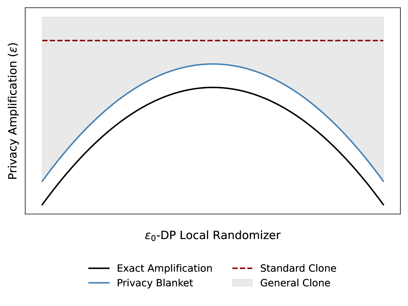
Figure 1. Hierarchy among decomposition-based methods

4.1. Definition of general clone

Definition 0 (Decomposition in the General Clone Paradigm).

Let $\mathcal{R}:\mathbb{X}\to\mathbb{Y}$ be a local randomizer. The general clone paradigm considers the following decomposition:

$$\mathcal{R}(x_{1}^{0}) =\sum_{j=1}^{k}a_{j}Q_{1}^{j},$$

$$\mathcal{R}(x_{1}^{1}) =\sum_{j=1}^{k}b_{j}Q_{1}^{j},$$

(2) $$\forall i\in[2,n],\quad\mathcal{R}(x_{i}) =\sum_{j=1}^{k}c_{j}Q_{1}^{j}+\beta Q_{i},$$

where $Q_{1}^{j}$ for $j=1,\dots,k$ and $Q_{i}$ for $i=2,\dots,n$ are probability distributions over $\mathbb{Y}$, and $a_{j},b_{j},c_{j},\beta$ are non-negative coefficients satisfying:

$$\sum_{j=1}^{k}a_{j}=1,\quad\sum_{j=1}^{k}b_{j}=1,\quad\sum_{j=1}^{k}c_{j}+\beta=1.$$

The general clone paradigm characterizes the general form of decompositions used in privacy amplification analysis. It directly subsumes the decomposition used in the standard clone framework. Although the decomposition defined by the privacy blanket appears structurally different, we will show that it naturally corresponds to a valid decomposition under the general clone paradigm.

When deriving the reduction pair from a general clone decomposition, an important constraint must be considered. Motivated by the failure of the stronger clone, the components $Q_{1}^{j}$ (shared across users) should not be mixed with the left-over distributions $Q_{i}$ (which are user-specific). This separation is essential to ensure the correctness and validity of the reduction.

Definition 0 (Reduction Pair of the General Clone).

Let $A_{0},A_{1}$, and $A_{2}$ be random variables on $\{1,2,\dots,k+1\}$, defined by the probabilities:

$$\Pr[A_{0}=j]=\begin{cases}a_{j}&\text{for }j\leq k,\\ 0&\text{for }j=k+1.\end{cases},\Pr[A_{1}=j]=\begin{cases}b_{j}&\text{for }j\leq k,\\ 0&\text{for }j=k+1.\end{cases}$$

$$\Pr[A_{2}=j]=\begin{cases}c_{j}&\text{for }j\leq k,\\ \beta&\text{for }j=k+1.\end{cases}$$

The reduction pair $(P_{0}^{GC},P_{1}^{GC})$ (with “GC” denoting “General Clone”) is defined as the distributions of the histograms over $\{1,\dots,k+1\}$ generated by sampling:

• One sample from $A_{0}$ for $P_{0}^{GC}$ (or $A_{1}$ for $P_{1}^{GC}$);

• $n-1$ i.i.d. samples from $A_{2}$.

The output is the histogram vector $(n_{1},n_{2},\dots,n_{k},n_{k+1})$ indicating the counts of each index.

4.2. General clone is not stronger than blanket

Given a specific randomizer, we compare any decomposition within the general clone paradigm against the decomposition provided by the privacy blanket framework.

Theorem 3.

For every local randomizer, there is a post-processing function from $(P_{0}^{GC},P_{1}^{GC})$ to the $(P_{0}^{B},P_{1}^{B})$, where $(P_{0}^{GC},P_{1}^{GC})$ is the reduction pair given by the general clone paradigm equipped with any decomposition, and $(P_{0}^{B},P_{1}^{B})$ is the reduction pair given by the privacy blanket framework. Therefore,

$$D_{e^{\epsilon}}(\mathcal{M}_{S}(X_{0}),\mathcal{M}_{S}(X_{1}))\leq D_{e^{\epsilon}}(P_{0}^{B},P_{1}^{B})\leq D_{e^{\epsilon}}(P_{0}^{GC},P_{1}^{GC}).$$

Proof.

The core idea of the proof is that the privacy blanket characterizes the maximal common part shared by all $\mathcal{R}(x_{i})$. The common part in any decomposition under the general clone paradigm cannot exceed that of the privacy blanket.

Recall the definition of $\omega(y)=\inf_{x\in\mathbb{X}}R(x)(y)/\gamma$, where $\gamma$ is a normalization factor. An important observation is that

$$\forall y\in\mathbb{Y}:\sum_{j=1}^{k}c_{j}Q_{1}^{j}(y)\leq\gamma\omega(y).$$

It is because the formula (2) should always hold for all $x_{2},x_{3},\dots,x_{n}\in\mathbb{X}$, i.e., $\forall x\in\mathbb{X}:\sum_{j=1}^{k}c_{j}Q_{1}^{j}(y)\leq R(x)(y)$. Hence, it follows that $\sum_{j=1}^{k}c_{j}\leq\gamma$ and $1-\gamma\leq\beta$. It means that each $Q_{i}$ can be decomposed by

$$Q_{i}=\frac{\gamma-\sum_{j=1}^{k}c_{j}}{\beta}Q^{com}+(1-\frac{\gamma-\sum_{j=1}^{k}c_{j}}{\beta})Q_{i}^{\prime},$$

where $Q^{com},Q_{i}^{\prime}$ are two probability distributions, $Q^{com}$ is the common part of all $Q_{i}$.

The function $f_{2}$ shown in Algorithm 3 is the post-processing function satisfying $f_{2}(P_{0}^{GC})=P_{0}^{B},f_{2}(P_{1}^{GC})=P_{1}^{B}$. It behaves as follows: when encountering an index $i\in[1,k]$, it samples from the corresponding distribution $Q_{1}^{i}$; when encountering $i=k+1$, it samples from the common distribution $Q^{\text{com}}$ with a certain probability. Taken together, this behavior is equivalent to each user (except the first) sampling from the blanket distribution with probability $\gamma$. ∎

As a result, although both $D_{e^{\epsilon}}(P_{0}^{GC}||P_{1}^{GC})$ and $D_{e^{\epsilon}}(P_{0}^{B}||P_{1}^{B})$ serve as upper bounds on the privacy amplification in the shuffle model, the bound provided by the privacy blanket is always at least as tight as that of the general clone paradigm under any decomposition.

4.3. Blanket is “in” the general clone

For every local randomizer, the general clone paradigm always admits a decomposition that is equivalent to the decomposition in the privacy blanket framework, where the components are single-point distributions $\mathbbm{1}_{y_{j}}$, with $y_{j}\in\mathbb{Y}$.

Theorem 4.

For every local randomizer, the following decomposition in the general clone paradigm is equivalent to the privacy blanket framework:

$$\mathcal{R}(x_{1}^{0}) =\sum_{j=1}^{|\mathbb{Y}|}a_{j}\mathbbm{1}_{y_{j}}$$

$$\mathcal{R}(x_{1}^{1}) =\sum_{j=1}^{|\mathbb{Y}|}b_{j}\mathbbm{1}_{y_{j}}$$

(3) $$\forall i\in[2,n],\quad\mathcal{R}(x_{i}) =\sum_{j=1}^{|\mathbb{Y}|}c_{j}\mathbbm{1}_{y_{j}}+\beta Q_{i}.$$

where $a_{j}=\mathcal{R}(x_{1}^{0})(y_{j})$, $b_{j}=\mathcal{R}(x_{1}^{1})(y_{j})$, and $c_{j}=\inf_{x\in\mathbb{X}}\mathcal{R}(x)(y_{j})$.

Proof.

It is straightforward to observe that $(P_{0}^{B},P_{1}^{B})$ and $(P_{0}^{GC},P_{1}^{GC})$ are essentially equivalent, differing only in some technical notations. ∎

We refer to the optimal decomposition of a local randomizer as the decomposition equivalent to that in the privacy blanket framework. For simplicity, we can merge some components to obtain an equally optimal decomposition. As an example, consider the $k$-Random Response mechanism.

Example 4.0.

Denote $\{1,2,\dots,k\}$ by $[k]$ and the uniform distribution on $[k]$ by $\mathcal{U}_{[k]}$. For any $k\in\mathbb{N}$ and $\varepsilon_{0}>0$, the $k$-randomized response mechanism $k\text{RR}:[k]\to[k]$ is defined as:

$$k\text{RR}(x)=\begin{cases}x,&\text{with probability }\frac{e^{\varepsilon_{0}}-1}{e^{\varepsilon_{0}}+k-1},\\ y\sim\mathcal{U}_{[k]},&\text{with probability }\frac{k}{e^{\varepsilon_{0}}+k-1}.\end{cases}$$

Its optimal decomposition is as follows:

$$R(x_{1}^{0}) =e^{\epsilon_{0}}p\mathbbm{1}_{x_{1}^{0}}+p\mathbbm{1}_{x_{1}^{1}}+qU,$$

$$R(x_{1}^{1}) =p\mathbbm{1}_{x_{1}^{0}}+e^{\epsilon_{0}}p\mathbbm{1}_{x_{1}^{1}}+qU,$$

$$\forall i\in[2,n]:R(x_{i}) =p\mathbbm{1}_{x_{1}^{0}}+p\mathbbm{1}_{x_{1}^{1}}+qU+(e^{\epsilon_{0}}-1)p\mathbbm{1}_{x_{i}}.$$

where $p=\frac{1}{e^{\epsilon_{0}}+k-1}$, $q=(k-2)p$, and $U$ is the uniform distribution over $[k]-\{x_{1}^{0},x_{1}^{1}\}$. This decomposition is also considered in the corrected version of the stronger clone (Feldman et al., 2023b).

The optimal decompositions for Binary Local Hash (Wang et al., 2017), Hadamard Response (Acharya et al., 2019), RAPPOR (Erlingsson et al., 2014), and Optimized Unary Encoding (OUE) (Wang et al., 2017) are provided in Appendix B.

Algorithm 3 Post-processing function from general clone paradigm to privacy blanket framework, $f_{2}$

$(n_{1},\dots,n_{k},n_{k+1})\in\{0,1,\dots,n\}^{k+1}$

$Y\leftarrow\emptyset$

for $i=1,\dots,k+1$ do

  for $count=1,2,\dots,n_{i}$ do

   if $i=k+1$ then

     $r\leftarrow\text{Bern}(\frac{\gamma-\sum_{j=1}^{k}c_{j}}{\beta})$

     if $r=1$ then

      $s\leftarrow_{Q^{com}}\mathbb{Y}$ $\triangleright$ Sample from $Q^{com}$

      $Y\leftarrow Y\cup\{s\}$

     end if

   else

     $s\leftarrow_{Q^{i}_{1}}\mathbb{Y}$ $\triangleright$ Sample from $Q^{i}_{1}$

     $Y\leftarrow Y\cup\{s\}$

   end if

  end for

end for

return $(|Y|-1,Y)$

5. Efficient Algorithm for Computing the Optimal Bounds

In this section, we present an efficient algorithm to compute the optimal privacy amplification bounds within the general clone framework. Our approach builds upon the previously overlooked concept of the privacy amplification random variable (PARV), originally proposed in the privacy blanket framework (Balle et al., 2019). While PARV offers an exact expression for the amplification bound, the original work did not provide a method for computing it precisely, relying instead on loose analytical approximations.

To overcome this limitation, we introduce the generalized privacy amplification random variable (GPARV), which enables precise and efficient numerical computation of the optimal bounds via Fast Fourier Transform (FFT).

In addition to computing upper bounds, our method can also be used to compute privacy amplification lower bounds, which serve as a reference for evaluating the tightness of the computed upper bounds. Experimental results (see Section 8) confirm that the gap between these upper and lower bounds is typically small, demonstrating the accuracy and effectiveness of our approach.

5.1. (Generalized) Privacy amplification random variable

Definition 0 (Privacy Amplification Random Variable (Balle et al., 2019)).

Suppose $W\sim\omega$ is a $\mathbb{Y}$-valued random variable sampled from the blanket. For any $\epsilon>0$ and $x,x^{\prime}\in\mathbb{X}$, the privacy amplification random variable is defined as

$$L^{x,x^{\prime}}_{\epsilon}=\frac{R(x)(W)-e^{\epsilon}R(x^{\prime})(W)}{\omega(W)}.$$

Using PARV, Balle et al. derived the precise expression for $D_{e^{\epsilon}}(P_{0}^{B}\|P_{1}^{B})$:

Lemma 2 (Lemma 5.3 in (Balle et al., 2019)).

Let $\mathcal{R}:\mathbb{X}\to\mathbb{Y}$ be a local randomizer and let $\mathcal{M}_{S}=\mathcal{S}\circ\mathcal{R}^{n}$ be the shuffling of $\mathcal{R}$. Fix $\varepsilon\geq 0$ and inputs $X^{0}\simeq X^{1}$ with $x_{1}^{0}\neq x_{1}^{1}$. Suppose $L_{1},L_{2},\dots$ are i.i.d. copies of $L_{\varepsilon}^{x_{1}^{0},x_{1}^{1}}$ and $\gamma$ is defined as in Section 3.2. Then, we have:

$$D_{e^{\epsilon}} (\mathcal{M}_{S}(X^{0})\|\mathcal{M}_{S}(X^{1}))$$

(4) $$\leq D_{e^{\epsilon}}(P_{0}^{B}\|P_{1}^{B})=\frac{1}{\gamma n}\sum_{m=1}^{n}\binom{n}{m}\gamma^{m}(1-\gamma)^{n-m}\mathbb{E}\left[\sum_{i=1}^{m}L_{i}\right]_{+}.$$

The bound above can also be expressed probabilistically as follows (Balle et al., 2019). Let $M\sim\text{Bin}(n,\gamma)$ be the random variable counting the number of users who sample from the blanket of $\mathcal{R}$. Formula (4) can be re-written as:

$$D_{e^{\epsilon}}(P_{0}^{B}\|P_{1}^{B})=\frac{1}{\gamma n}\mathbb{E}_{M\sim\text{Bin}(n,\gamma)}\left[\sum_{i=1}^{M}L_{i}\right]_{+},$$

where we use the convention $\sum_{i=1}^{m}L_{i}=0$ when $m=0$.

Unfortunately, Balle et al. stopped at this point and did not pursue further simplification. In the following, we demonstrate how to improve upon the PARV to enable precise computation.

Definition 0 (Generalized Privacy Amplification Random Variable (GPARV)).

Define the generalized privacy amplification random variable as:

$$\text{G}_{\epsilon}^{x,x^{\prime}}=\begin{cases}\frac{1}{\gamma}L_{\epsilon}^{x,x^{\prime}},&\text{w.p.}\ \gamma,\\ 0,&\text{w.p.}\ 1-\gamma.\end{cases}$$

where $L_{\epsilon}^{x,x^{\prime}}$ is defined in Definition 1.

We can now restate Lemma 2 in a simplified form:

Theorem 4.

Let $\mathcal{R}:\mathbb{X}\to\mathbb{Y}$ be a local randomizer and let $\mathcal{M}_{S}=\mathcal{S}\circ\mathcal{R}^{n}$ be the shuffling of $\mathcal{R}$. Fix $\varepsilon\geq 0$ and inputs $X^{0}\simeq X^{1}$ with $x_{1}^{0}\neq x_{1}^{1}$. Suppose $G_{1},G_{2},\dots$ are i.i.d. copies of $G_{\varepsilon}^{x_{1}^{0},x_{1}^{1}}$ and $\gamma$ is defined as in Section 3.2. Then, we have:

$$D_{e^{\epsilon}}(\mathcal{M}_{S}(X^{0})\|\mathcal{M}_{S}(X^{1}))\leq D_{e^{\epsilon}}(P_{0}^{B}\|P_{1}^{B})=\frac{1}{n}\mathbb{E}\left[\sum_{i=1}^{n}G_{i}\right]_{+}.$$

The GPARV has the following properties:

Property 2.

Let $\mathcal{R}:\mathbb{X}\to\mathbb{Y}$ be an $\varepsilon_{0}$-LDP local randomizer. For any $\varepsilon\geq 0$ and $x,x^{\prime}\in\mathbb{X}$, the generalized privacy amplification random variable $G=G_{\varepsilon}^{x,x^{\prime}}$ satisfies:

1. $\mathbb{E}[G]=1-e^{\epsilon}$,

2. $1-e^{\epsilon+\epsilon_{0}}\leq G\leq e^{\epsilon_{0}}-e^{\epsilon}$.

Proof.

The first property follows from direct computation:

$$\mathbb{E}[G]=\gamma\mathbb{E}\left[\frac{1}{\gamma}L\right]=\mathbb{E}[L]=\mathbb{E}_{W\sim\omega}\left[\frac{R(x)(W)-e^{\epsilon}R(x^{\prime})(W)}{\omega(W)}\right]=1-e^{\epsilon}.$$

The second property is due to the $\epsilon_{0}$-DP property of $R$: $\forall x\in\mathbb{X},y\in\mathbb{Y}:1\leq\frac{R(x)(y)}{\gamma\omega(y)}\leq e^{\epsilon_{0}}$, so

$$1-e^{\epsilon+\epsilon_{0}}\leq\frac{R(x)(W)-e^{\epsilon}R(x^{\prime})(W)}{\gamma\omega(W)}\leq e^{\epsilon_{0}}-e^{\epsilon}.\qed$$

Remark 1.

In the original paper of the privacy blanket framework, a similar property of PARV was provided, but in a loose form (Balle et al., 2019). Specifically, they established that $\gamma(e^{-\epsilon_{0}}-e^{\epsilon+\epsilon_{0}})\leq L\leq\gamma(e^{\epsilon_{0}}-e^{\epsilon-\epsilon_{0}})$. However, the $\epsilon_{0}$-DP property of $R$ actually guarantees a tighter bound: $\gamma(1-e^{\epsilon+\epsilon_{0}})\leq L\leq\gamma(e^{\epsilon_{0}}-e^{\epsilon})$.

5.2. Algorithm for computing privacy amplification upper bounds

We present a new algorithm for computing the optimal privacy amplification bound under the general clone paradigm for any specific local randomizer, as described in Algorithm 4.

Overview.

First, the distribution of the generalized privacy amplification random variable (GPARV) $G_{\epsilon}^{x,x^{\prime}}$ is computed for a given local randomizer. Since most local randomizers exhibit input symmetry, the distribution of $G$ typically does not depend on the specific values of $x$ and $x^{\prime}$. We thus denote it simply by $G_{\epsilon}$. The distributions of $G_{\epsilon}$ for commonly used local randomizers are summarized in Table 1. The distribution of $G_{\epsilon}$ for Laplace mechanism is presented in Appendix C.

Given the distribution of $G_{\epsilon}$, our algorithm discretizes it to obtain $\bar{G}$, by rounding each value in $G$ up to the nearest larger multiple of a discretization interval length $l$:

$$\text{Round}(x)=l\cdot\lceil\frac{x}{l}\rceil.$$

Next, the algorithm computes the $n$-fold convolution of $\bar{G}$, denoted $\bar{G}^{*n}$, using the classical Fast Fourier Transform method:

$$\bar{G}^{*n}=\text{FFT}^{-1}\left((\text{FFT}(\bar{G}))^{\odot n}\right),$$

where $\odot n$ represents the element-wise exponentiation by $n$.

Finally, the algorithm evaluates the integral

$$I=\mathbb{E}[\bar{G}^{*n}]_{+}=\int_{0}^{+\infty}x\,\bar{G}^{*n}(x)\,dx,$$

and outputs $\frac{I}{n}$ as the upper bound on privacy amplification.

Correctness.

The output of the algorithm is guaranteed to upper bound the true value, since the discretized distribution $\bar{G}$ stochastically dominates $G$:

$$\frac{1}{n}\mathbb{E}[\bar{G}^{*n}]_{+}\geq\frac{1}{n}\mathbb{E}[G^{*n}]_{+}.$$

Time Complexity and Error Analysis.

Because $G$ is supported on the interval $[1-e^{\epsilon_{0}+\epsilon},e^{\epsilon_{0}}-e^{\epsilon}]$ (Property 2), the discretization step requires $O\left(\frac{e^{\epsilon_{0}+\epsilon}}{l}\right)$ operations. For most frequency oracles used on categorical data, $G$ takes values on at most five points (see Table 1), resulting in $O(1)$ discretization time.

The discretization introduces a bounded error. An intuitive analysis is as follows:

$$\mathbb{E}[\bar{G}^{*n}]_{+}-nl\leq\mathbb{E}[G^{*n}]_{+}\leq\mathbb{E}[\bar{G}^{*n}]_{+}.$$

The FFT computation runs in $O\left(\frac{n}{l}\log\left(\frac{n}{l}\right)\right)=\widetilde{O}(\frac{n}{l})$ time. Choosing $l=O\left(\frac{1}{n}\right)$ ensures an $O(1)$ additive error in total $\widetilde{O}(n^{2})$ time.

More precise analysis can be done:

$$\mathbb{E}[\bar{G}^{*n}]_{+}-nl\cdot\Pr\left[[G^{*n}]_{+}>-nl\right]\leq\mathbb{E}[G^{*n}]_{+}\leq\mathbb{E}[\bar{G}^{*n}]_{+}.$$

By Hoeffding’s inequality,

$$\Pr\left[[G^{*n}]_{+}>-nl\right]\leq\exp\left(-\left(\frac{2a^{2}}{b^{2}}-l\right)n\right),$$

where $a=-\mathbb{E}[G]=e^{\epsilon}-1$ and $b=(e^{\epsilon_{0}}-1)(e^{\epsilon}+1)$. This shows that the error decays exponentially in $n$ as long as $l\leq\frac{2a^{2}}{b^{2}}$. Empirical evaluations confirm that $l=O(1)$ is sufficiently accurate in practice (see Section 8), and the overall FFT runtime becomes $O(n\log n)$.

Comparison with Existing Numerical Methods.

The numerical computation of privacy amplification in the shuffle model has been studied since the introduction of the clone paradigm by Feldman et al. (Feldman et al., 2022). Prior numerical algorithms can only handle three-point decompositions, such as computing $D_{e^{\epsilon}}(P_{0}^{C}\|P_{1}^{C})$ (Feldman et al., 2022; Wang et al., 2024; Koskela et al., 2021). However, these techniques do not generalize to decompositions involving more than three points, which are essential for obtaining tight bounds from optimal decompositions.

In contrast, our FFT-based algorithm supports the optimal decomposition of any local randomizer, enabling tighter and more accurate privacy amplification bounds. Furthermore, our method is not only more general but also simpler and significantly faster than existing numerical algorithms (see Section 8).

Table 1. The probability distribution of GPARV for common LDP protocols

	$1-e^{\epsilon_{0}+\epsilon}$	$e^{\epsilon_{0}}-e^{\epsilon_{0}+\epsilon}$	$1-e^{\epsilon}$	0	$e^{\epsilon_{0}}-e^{\epsilon}$
$k$-RR (Warner, 1965)	$\frac{1}{e^{\epsilon_{0}}+k-1}$	0	$\frac{k-2}{e^{\epsilon_{0}}+k-1}$	$\frac{e^{\epsilon_{0}}-1}{e^{\epsilon_{0}}+k-1}$	$\frac{1}{e^{\epsilon_{0}}+k-1}$
BLH (Wang et al., 2017)	$\frac{1}{2(e^{\epsilon_{0}}+1)}$	$\frac{1}{2(e^{\epsilon_{0}}+1)}$	$\frac{1}{2(e^{\epsilon_{0}}+1)}$	$\frac{e^{\epsilon_{0}}-1}{e^{\epsilon_{0}}+1}$	$\frac{1}{2(e^{\epsilon_{0}}+1)}$
RAPPOR (Erlingsson et al., 2014)	$\frac{1}{(e^{\epsilon_{0}/2}+1)^{2}}$	$\frac{1}{e^{\epsilon_{0}/2}(e^{\epsilon_{0}/2}+1)^{2}}$	$\frac{e^{\epsilon_{0}/2}}{(e^{\epsilon_{0}/2}+1)^{2}}$	$1-e^{-\epsilon_{0}/2}$	$\frac{1}{(e^{\epsilon_{0}/2}+1)^{2}}$
OUE (Wang et al., 2017)	$\frac{1}{2(e^{\epsilon_{0}}+1)}$	$\frac{1}{2e^{\epsilon_{0}}(e^{\epsilon_{0}}+1)}$	$\frac{e^{\epsilon_{0}}}{2(e^{\epsilon_{0}}+1)}$	$\frac{1}{2}(1-e^{-\epsilon_{0}})$	$\frac{1}{2(e^{\epsilon_{0}}+1)}$
HR (Acharya et al., 2019)	$\frac{1}{2(e^{\epsilon_{0}}+1)}$	$\frac{1}{2(e^{\epsilon_{0}}+1)}$	$\frac{1}{2(e^{\epsilon_{0}}+1)}$	$\frac{e^{\epsilon_{0}}-1}{e^{\epsilon_{0}}+1}$	$\frac{1}{2(e^{\epsilon_{0}}+1)}$

Algorithm 4 Calculate the optimal privacy amplification bound via FFT

the distritbuion density $G$ of $G_{\epsilon}$, number of users $n$, discretisation interval length $l$

$\bar{G}=$ Discretize($G$,$l$) $\triangleright$ Round every point of $G$ to $nl,n\in\mathbb{Z}$

$\bar{G}^{*}=\text{FFT}^{-1}((\text{FFT}(\bar{G}))^{\odot n})$  $\triangleright$ Compute the $n$-fold convolution

$I\leftarrow\int_{0}^{+\infty}x\bar{G}^{*}(x)dx$ $\triangleright$ Compute the integral

return $\frac{I}{n}$

5.3. Algorithm for computing privacy amplification lower bounds

Our generalized privacy amplification random variable (GPARV) also facilitates the computation of lower bounds for privacy amplification via shuffling. These bounds help to demonstrate the tightness of the upper bounds.

An upper bound refers to the existence of a value $\delta_{u}$ such that, for a given local randomizer with specified $\epsilon_{0},\epsilon,n$, and for any two neighboring input datasets $X^{0}$ and $X^{1}$, we have:

$$D_{e^{\epsilon}}\big{(}\mathcal{M}_{S}(X^{0}),\mathcal{M}_{S}(X^{1})\big{)}\leq\delta_{u}.$$

For a given local randomizer with specified $\epsilon_{0},\epsilon,n$, we can construct two neighboring datasets $X^{0}$ and $X^{1}$, and compute:

$$\delta_{l}=D_{e^{\epsilon}}\big{(}\mathcal{M}_{S}(X^{0}),\mathcal{M}_{S}(X^{1})\big{)},$$

which serves as the lower bound for this amplification.

In previous studies, a common strategy for selecting neighboring datasets $X^{0}$ and $X^{1}$ is to set $x_{2}=x_{3}=\dots=x_{n}$, such that $x_{1}^{0}$, $x_{1}^{1}$, and $x_{2}$ are mutually distinct (Feldman et al., 2023a; Wang et al., 2024). In the special case where $|\mathbb{X}|=2$, the datasets $X^{0}$ and $X^{1}$ can be chosen as

$$x_{1}^{0}\neq x_{1}^{1},\quad\text{and}\quad x_{2}=x_{3}=\dots=x_{n}=x_{1}^{1}.$$

For the Laplace mechanism with continuous domain $\mathbb{X}=[a,b]$, a natural choice is

$$x_{1}^{0}=a,\quad x_{1}^{1}=b,\quad\text{and}\quad x_{2}=x_{3}=\dots=x_{n}=\frac{a+b}{2}.$$

The following theorem provides an efficient method for computing the hockey-stick divergence $D_{e^{\epsilon}}\big{(}\mathcal{M}_{S}(X^{0}),\mathcal{M}_{S}(X^{1})\big{)}$ under this setting.

Theorem 5.

Let $\mathcal{R}:\mathbb{X}\to\mathbb{Y}$ be a local randomizer, and let $\mathcal{M}_{S}=\mathcal{S}\circ\mathcal{R}^{n}$ be the shuffling of $\mathcal{R}$. Fix $\varepsilon\geq 0$ and inputs $X^{0}\simeq X^{1}$ with $x_{1}^{0}\neq x_{1}^{1}$ and $x_{2}=x_{3}=\dots=x_{n}$. Define a random variable $G=\frac{\mathcal{R}(x_{1}^{0})(y)-e^{\epsilon}\mathcal{R}(x_{1}^{1})(y)}{\mathcal{R}(x_{2})(y)}$, where $y\sim\mathcal{R}(x_{2})$. Suppose $G_{1},G_{2},\dots$ are i.i.d. copies of $G$. Then, we have the following:

$$D_{e^{\epsilon}}(\mathcal{M}_{S}(X^{0})\|\mathcal{M}_{S}(X^{1}))=\frac{1}{n}\mathbb{E}\left[\sum_{i=1}^{n}G_{i}\right]_{+}.$$

We provide the proof in Appendix D. The result indicates that, for $X^{0}$ and $X^{1}$ satisfying $x_{2}=x_{3}=\dots=x_{n}$, we can efficiently compute $D_{e^{\epsilon}}\big{(}\mathcal{M}_{S}(X^{0}),\mathcal{M}_{S}(X^{1})\big{)}$ using FFT.

6. Joint Composition of LDP

In this section, we analyze the joint composition of multiple LDP local randomizers $\mathcal{R}_{1},\mathcal{R}_{2},\dots,\mathcal{R}_{m}$. Let $\mathcal{R}_{i}:\mathbb{X}^{i}\to\mathbb{Y}^{i}$ denote the local randomizer for the $i$-th component. The joint composition of these randomizers is defined as follows:

$$\mathcal{R}^{\times}_{[1:m]}:\mathbb{X}^{1}\times\mathbb{X}^{2}\times\dots\times\mathbb{X}^{m}\to\mathbb{Y}^{1}\times\mathbb{Y}^{2}\times\dots\times\mathbb{Y}^{m},$$

$$\mathcal{R}^{\times}_{[1:m]}(x_{1},x_{2},\dots,x_{m})=(\mathcal{R}_{1}(x_{1}),\mathcal{R}_{2}(x_{2}),\dots,\mathcal{R}_{m}(x_{m})).$$

We assume that any two input vectors $\boldsymbol{x}=(x_{1},x_{2},\dots,x_{m})$ and $\boldsymbol{x}^{\prime}=(x_{1}^{\prime},x_{2}^{\prime},\dots,x_{m}^{\prime})$ are neighboring. In practice, it is common to use the joint composition of $m$ mechanisms, each satisfying $\left(\frac{\epsilon_{0}}{m}\right)$-LDP, to achieve overall $\epsilon_{0}$-LDP.

Theorem 1 (Joint Composition Theorem).

If $\mathcal{R}_{i}$ satisfies $\epsilon_{i}$-LDP, then $\mathcal{R}^{\times}_{[1:m]}$ satisfies $\sum_{i=1}^{m}\epsilon_{i}$-LDP.

When applied to LDP protocols resulting from joint composition, the clone paradigm provides particularly loose decompositions. This is due to the presence of many intermediate states in the joint probability distribution after the composition. For instance, most local randomizers have probability ratios between any two inputs that belong to the set $\{e^{-\epsilon_{0}},1,e^{\epsilon_{0}}\}$. However, after a $m$-fold joint composition, the ratio of the joint probability distribution may belong to $\{e^{i\epsilon_{0}}|i\in[-m,m]\cap\mathbb{Z}\}$. Under these conditions, the common part in the clone paradigm deviates significantly from the actual privacy blanket.

To compute the optimal privacy amplification bound, we only need to compute the GPARV of $\mathcal{R}^{\times}_{[1:m]}$, which is equivalent to finding the optimal decomposition of $\mathcal{R}^{\times}_{[1:m]}$. Fortunately, the optimal decomposition of a joint composition mechanism is simply the Cartesian product of the optimal decompositions of each individual LDP component.

As an example, consider the joint composition of two $k$-RR mechanisms acting on $[k]\times[k]$. The optimal decomposition is given below:

Example 6.0 (Optimal Decomposition of Two-Joint $k$-RR).

$$\mathcal{R}^{\times}(a_{1}^{0},b_{1}^{0})=\left(e^{\epsilon_{0}/2}p\mathbbm{1}_{a_{1}^{0}}+p\mathbbm{1}_{a_{1}^{1}}+qU\right)\times\left(e^{\epsilon_{0}/2}p\mathbbm{1}_{b_{1}^{0}}+p\mathbbm{1}_{b_{1}^{1}}+qU\right),$$

$$\mathcal{R}^{\times}(a_{1}^{1},b_{1}^{1})=\left(p\mathbbm{1}_{a_{1}^{0}}+e^{\epsilon_{0}/2}p\mathbbm{1}_{a_{1}^{1}}+qU\right)\times\left(p\mathbbm{1}_{b_{1}^{0}}+e^{\epsilon_{0}/2}p\mathbbm{1}_{b_{1}^{1}}+qU\right),$$

$$\forall i\in[2,n],\ \mathcal{R}^{\times}(a_{i},b_{i})=\left(p\mathbbm{1}_{a_{1}^{0}}+p\mathbbm{1}_{a_{1}^{1}}+qU+(1-2p-q)\mathbbm{1}_{a_{i}}\right)$$

$$\quad\times\left(p\mathbbm{1}_{b_{1}^{0}}+p\mathbbm{1}_{b_{1}^{1}}+qU+(1-2p-q)\mathbbm{1}_{b_{i}}\right)$$

where $p=\frac{1}{e^{\epsilon_{0}/2}+k-1}$, $q=\frac{k-2}{e^{\epsilon_{0}/2}+k-1}$, and $U$ is the uniform distribution over $[k]-\{a_{1}^{0},a_{1}^{1}\}$. The Cartesian product of two probability distributions $P,Q$ is defined as $(P\times Q)(a,b)=P(a)\cdot Q(b)$.

The optimal decompositions of other jointly composed local randomizers can be computed in a similar manner. For simplicity, all examples and experiments in this paper consider the joint composition of multiple instances of the same type of local randomizer, each with the same privacy parameter $\epsilon_{0}$. However, the Cartesian product approach described above naturally generalizes to joint compositions involving different types of local randomizers, each potentially with a different value of $\epsilon_{0}$.

7. Parallel Composition of LDP

The joint composition setting discussed earlier is well-suited for analyzing the joint distribution of multiple attributes associated with each user. In contrast, when each user possesses only a single attribute but the analyst aims to compute multiple statistical queries (each corresponding to a different local mechanism $\mathcal{R}_{1},\dots,\mathcal{R}_{m}$), a more appropriate strategy is parallel composition. It is defined as:

$$\mathcal{R}_{[1,m]}^{\parallel,\boldsymbol{p}}(x)=(i,\mathcal{R}_{i}(x)),w.p.\ p_{i},\quad i=1,2,\dots,m$$

where $\boldsymbol{p}=(p_{1},\dots,p_{m})$ is a probability vector with $\sum_{i=1}^{m}p_{i}=1$.

Theorem 1.

If $\mathcal{R}_{i}$ satisfies $\epsilon$-LDP, then $\mathcal{R}_{[1,m]}^{\parallel,\boldsymbol{p}}$ satisfies $\epsilon$-LDP.

Parallel composition partitions the user population into $m$ non-overlapping subsets and assigns each subset to one of the $m$ estimation tasks. Each subset can then utilize the full privacy budget $\varepsilon_{0}$, rather than dividing the budget across all tasks. This technique has been widely adopted in the literature (Bassily et al., 2017; Wang et al., 2019b, a, 2021; Cormode et al., 2018b) for achieving better utility than direct budget splitting.

To compute the optimal privacy amplification bound under parallel composition, we need to compute the GPARV of $\mathcal{R}^{\parallel,\boldsymbol{p}}_{[1:m]}$, which is equivalent to identifying its optimal decomposition. It is straightforward to show that the optimal decomposition of $\mathcal{R}^{\parallel,\boldsymbol{p}}_{[1:m]}$ is a weighted mixture of the optimal decompositions of each individual local randomizer $\mathcal{R}_{i}$, weighted by $p_{i}$.

For instance, suppose the optimal decompositions of $\mathcal{R}_{1}$ and $\mathcal{R}_{2}$ are given by the coefficients $a_{j},b_{j},c_{j},\beta_{1}$ for $j\in[k_{1}]$, and $d_{j},e_{j},f_{j},\beta_{2}$ for $j\in[k_{2}]$, respectively:

$$\mathcal{R}_{1}(x_{1}^{0}) =\sum_{j=1}^{k_{1}}a_{j}Q_{1}^{j}, \quad\mathcal{R}_{2}(x_{1}^{0}) =\sum_{j=1}^{k_{2}}d_{j}T_{1}^{j},$$

$$\mathcal{R}_{1}(x_{1}^{1}) =\sum_{j=1}^{k_{1}}b_{j}Q_{1}^{j}, \quad\mathcal{R}_{2}(x_{1}^{1}) =\sum_{j=1}^{k_{2}}e_{j}T_{1}^{j},$$

$$\forall i\in[2,n],\mathcal{R}_{1}(x_{i}) =\sum_{j=1}^{k_{1}}c_{j}Q_{1}^{j}+\beta_{1}Q_{i}, \quad\mathcal{R}_{2}(x_{i}) =\sum_{j=1}^{k_{2}}f_{j}T_{1}^{j}+\beta_{2}T_{i}.$$

Then, the optimal decomposition of $\mathcal{R}^{\parallel,\boldsymbol{p}}_{[1:2]}$ with $\boldsymbol{p}=(p_{1},p_{2})$ is:

$$\mathcal{R}^{\parallel}(x_{1}^{0}) =p_{1}\sum_{j=1}^{k_{1}}a_{j}Q_{1}^{j}+p_{2}\sum_{j=1}^{k_{2}}d_{j}T_{1}^{j},$$

$$\mathcal{R}^{\parallel}(x_{1}^{1}) =p_{1}\sum_{j=1}^{k_{1}}b_{j}Q_{1}^{j}+p_{2}\sum_{j=1}^{k_{2}}e_{j}T_{1}^{j},$$

$$\forall i\in[2,n],\ \mathcal{R}^{\parallel}(x_{i}) =p_{1}\left(\sum_{j=1}^{k_{1}}c_{j}Q_{1}^{j}+\beta_{1}Q_{i}\right)+p_{2}\left(\sum_{j=1}^{k_{2}}f_{j}T_{1}^{j}+\beta_{2}T_{i}\right).$$

8. Numerical Experiments

In this section, we conduct experimental evaluations of our FFT-based numerical algorithm proposed in this paper.

We compare the optimal bounds for specific local randomizers under the general clone paradigm with existing bounds. The baselines include two bounds from the privacy blanket framework, derived using Hoeffding’s and Bennett’s inequalities, respectively (Balle et al., 2019), as well as the numerical bounds from the standard clone paradigm (Feldman et al., 2022). We utilized the open-source implementations released by the respective papers.

We present results for five commonly used local randomizers: $k$-Randomized Response (Warner, 1965) ($k=10$), Binary Local Hash (Wang et al., 2017), RAPPOR (Erlingsson et al., 2014), Optimized Unary Encoding (OUE) (Wang et al., 2017) and Laplace mechanism (Dwork, 2006). The experimental results are shown in Figure 2 and Figure 3. The lower bounds are computed using the method described in Section 5.3. In the legends of the plots, “$k$-joint” refers to the joint composition of $k$ local randomizers, each satisfying $\frac{\epsilon_{0}}{k}$-LDP. In the experiments, the discretization interval length $l$ used in our FFT algorithm is set as $\frac{e^{\epsilon_{0}}-1}{1200}$ when $\epsilon_{0}=0.1$, and $\frac{e^{\epsilon_{0}}-1}{1000}$ when $\epsilon_{0}=4.0$. Due to space constraints, we present the results of the parallel composition in Appendix E.

The experimental results show that our upper bounds consistently outperform existing methods. Furthermore, the gap between our upper and lower bounds is generally small, indicating the tightness and reliability of the computed results. This also validates that our choice of discretization interval length $l$ offers sufficient precision for practical use.

In addition to its accuracy, our algorithm is highly efficient: it generates a full curve in approximately 30 seconds, whereas the numerical algorithm used for the standard clone requires around 5 minutes. It is worth noting that the numerical generic bound of the standard clone is weaker than the specific one provided by the privacy blanket using Bennett’s inequality in our experiments.

Our results show that computing bounds specific to joint compositions leads to significantly tighter amplification bounds compared to generic methods. This highlights the importance and advantage of our algorithm in accurately analyzing privacy in practical multi-attribute settings. Furthermore, we observe that, under a fixed total privacy budget $\epsilon_{0}$, the privacy amplification effect achieved through shuffling becomes stronger as the number of composed randomizers $k$ increases.

10-RR, low $\epsilon_{0}$

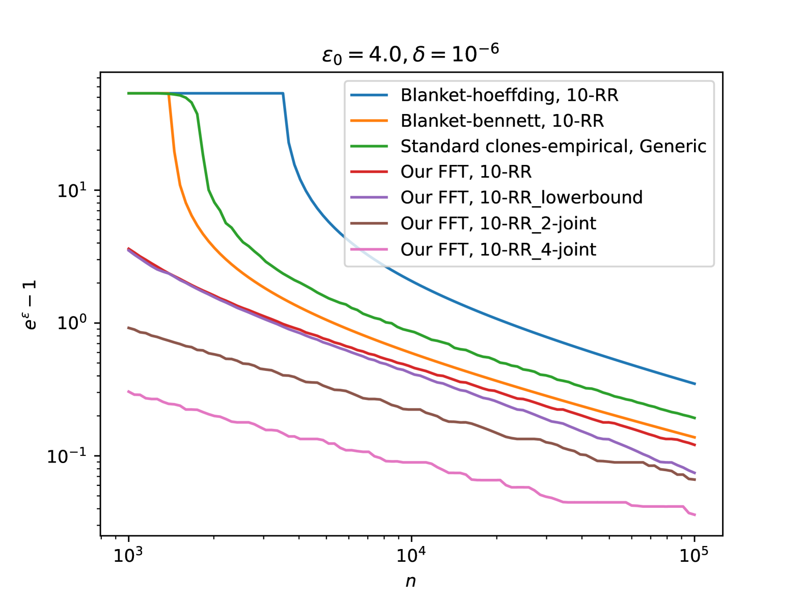
10-RR, large $\epsilon_{0}$

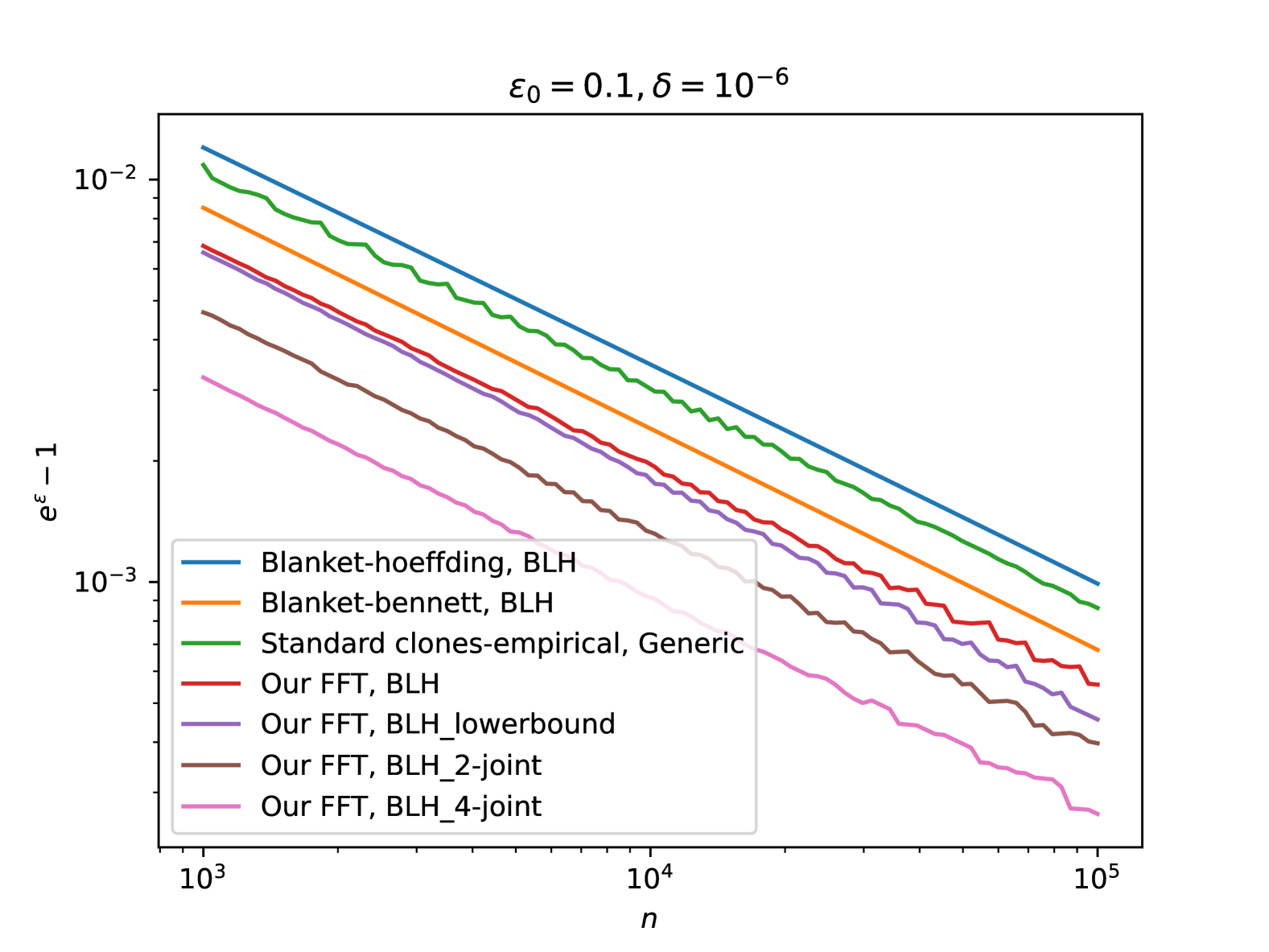
BLH, low $\epsilon_{0}$

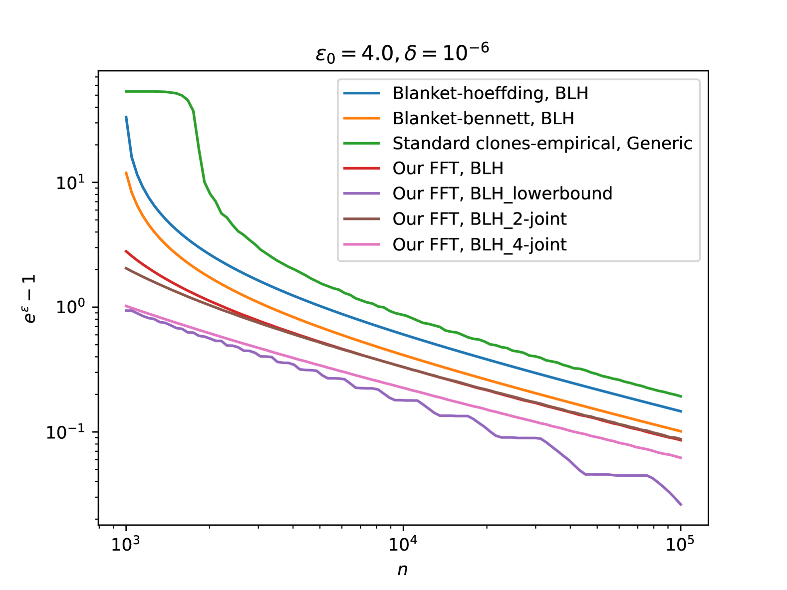
BLH, large $\epsilon_{0}$

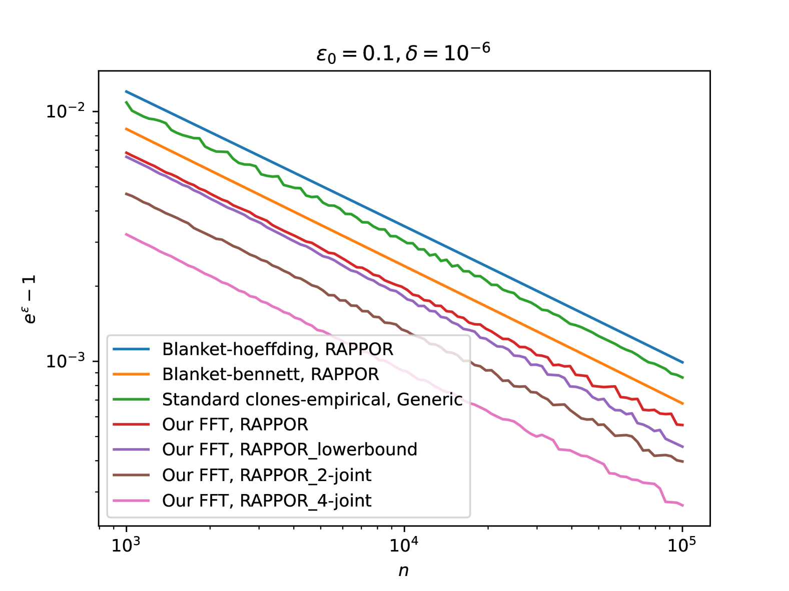
RAPPOR, low $\epsilon_{0}$

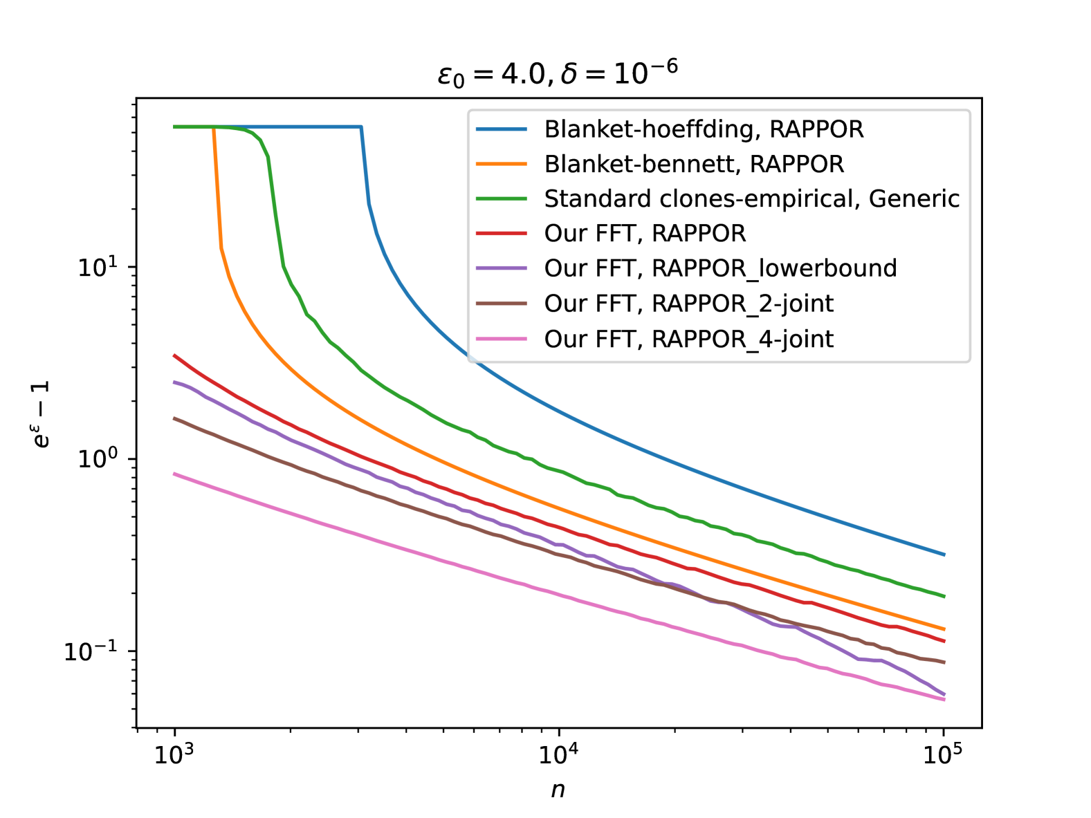
RAPPOR, large $\epsilon_{0}$

Figure 2. Experimental Results: RR, BLH and RAPPOR

OUE, low $\epsilon_{0}$

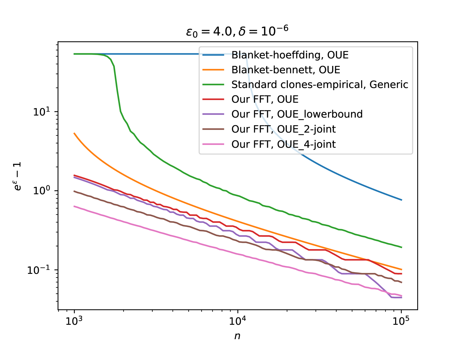
OUE, large $\epsilon_{0}$

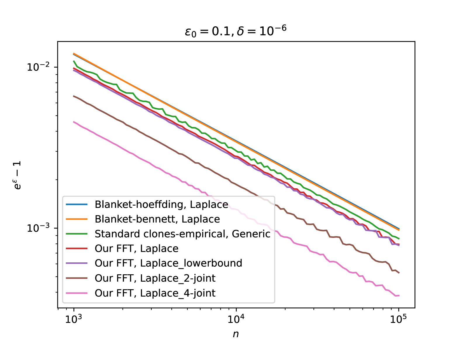
Laplace, low $\epsilon_{0}$

Laplace, large $\epsilon_{0}$

Figure 3. Experimental Results: OUE and Laplace

9. Discussion: Beyond the General Clone

In this work, we develop an efficient algorithm to compute the best-known privacy amplification bounds within the general clone framework, which encompasses all possible decompositions. A natural and important question arises: Can we achieve tighter bounds than those provided by the general clone? Addressing this question requires stepping beyond decomposition methods.

A promising direction is to identify the most vulnerable neighboring dataset pair $(X^{0},X^{1})$ such that $D_{e^{\epsilon}}\left(\mathcal{M}_{S}(X^{0}),\mathcal{M}_{S}(X^{1})\right)$ is maximized among all neighboring pairs of size $n$. If, for a local randomizer $\mathcal{R}$, one can prove that a specific pair $(X^{0}_{v},X^{1}_{v})$ consistently maximizes the divergence for every $\epsilon$, then this would yield the exact privacy amplification bound for $\mathcal{R}$ under shuffling.

For many local randomizers, a plausible candidate for the most vulnerable dataset pair is

$$X^{0}=(x_{1}^{0},x_{2},x_{2},\dots,x_{2}),\quad X^{1}=(x_{1}^{1},x_{2},x_{2},\dots,x_{2}),$$

where $x_{1}^{0},x_{1}^{1},x_{2}\in\mathbb{X}$ are mutually distinct. This construction is also used in Section 5.3 for computing lower bounds of privacy amplification.

This conjecture is motivated by two observations. First, to maximize distinguishability, the set of inputs $\{x_{i}\mid i=2,3,\dots,n\}$ should exclude both $x_{1}^{0}$ and $x_{1}^{1}$, ensuring that the outputs are not easily confounded. Second, having unified inputs among the remaining users simplifies the inference of their output contributions, thereby potentially increasing the overall distinguishability between the shuffled outputs of $X^{0}$ and $X^{1}$.

Despite its intuitive appeal, this conjecture currently lacks a formal proof. Developing tools to rigorously establish the most vulnerable neighboring pair remains an open problem and a valuable direction for future research.

10. Conclusion

In this work, we propose the general clone framework, which encompasses all decomposition methods, and identify the optimal bounds within the general clone framework. We also present an efficient algorithm for numerically computing these optimal bounds. With these results, we achieve the best-known bounds. Experiments demonstrate the tightness of our analysis. Additionally, we present methods for computing optimal amplification bounds for both joint composition and parallel composition in the shuffle model. We hope that this work contributes to both the practical deployment and the theoretical advancement of the shuffle model in differential privacy.

Appendix A Misunderstanding of the Privacy Blanket Framework

In this section, we discuss and correct a misunderstanding in the literature regarding the privacy blanket framework (Koskela et al., 2021).

The original paper on the privacy blanket framework demonstrates its usage with the example of $k$-Random Response (see Definition 5) (Balle et al., 2019). The privacy blanket distribution for $k$-RR is simply the uniform distribution over $[k]$. Let $N_{0}$ and $N_{1}$ denote the counts of $x_{1}^{0}$ and $x_{1}^{1}$ appearing in $Y_{|\boldsymbol{b}|}$ (see Definition 4), respectively. When $b_{1}=1$, it is easy to see that

$$\Pr[P_{0}^{B}(|\boldsymbol{b}|,Y_{|\boldsymbol{b}|})\mid b_{1}=1]=\Pr[P_{1}^{B}(|\boldsymbol{b}|,Y_{|\boldsymbol{b}|})\mid b_{1}=1].$$

When $b_{1}=0$, the first user commits their true value, i.e., $y_{1}^{b}=x_{1}^{b}$. In this case, using combinatorial analysis, we can derive the following (Balle et al., 2019):

$$\forall Y_{|\boldsymbol{b}|}:\quad\frac{\Pr[P_{0}^{B}(|\boldsymbol{b}|,Y_{|\boldsymbol{b}|})\mid b_{1}=0]}{\Pr[P_{1}^{B}(|\boldsymbol{b}|,Y_{|\boldsymbol{b}|})\mid b_{1}=0]}=\frac{N_{0}}{N_{1}}.$$

The mistake in (Koskela et al., 2021) lies in their characterization of the joint distribution of $N_{0}$ and $N_{1}$:

$$N_{0}\sim\text{Bin}(n-1,\frac{1}{e^{\epsilon}+k-1})+1\text{ and }N_{1}\sim\text{Bin}(n-1,\frac{1}{e^{\epsilon}+k-1})$$

under the condition $b_{1}=0$ and $(|\boldsymbol{b}|,Y_{|\boldsymbol{b}|})\sim P_{0}^{B}$. In reality, $N_{0}$ and $N_{1}$ are not independent, as also noted in (Luo et al., 2022). The correct characterization is as follows: let $N\sim\text{Bin}(n-1,\frac{k}{e^{\epsilon_{0}}+k-1})$, then $N_{0}\sim\text{Bin}(N,\frac{1}{k})+1$, and $N_{1}\sim\text{Bin}(N-N_{0},\frac{1}{k-1})$.

This mistake affects both the theoretical analysis and the experimental results reported in (Koskela et al., 2021).

Appendix B Optimal Decompositions for Common Local Randomizers

The optimal decompositions for common local randomizers involve five components with different coefficients, expressed as follows:

$$\mathcal{R}(x_{1}^{0}) =e^{\epsilon_{0}}p\mathcal{Q}_{1}^{0}+p\mathcal{Q}_{1}^{1}+e^{\epsilon_{0}}q\mathcal{Q}_{1}^{2}+r\mathcal{Q}_{1}^{3},$$

$$\mathcal{R}(x_{1}^{1}) =p\mathcal{Q}_{1}^{0}+e^{\epsilon_{0}}p\mathcal{Q}_{1}^{1}+e^{\epsilon_{0}}q\mathcal{Q}_{1}^{2}+r\mathcal{Q}_{1}^{3},$$

$$\forall i\in[2,n],\ \mathcal{R}(x_{i}) =p\mathcal{Q}_{1}^{0}+p\mathcal{Q}_{1}^{1}+q\mathcal{Q}_{1}^{2}+r\mathcal{Q}_{1}^{3}+(1-2p-q-r)\mathcal{Q}_{i}.$$

The values of the coefficients $p,q,r$ for several widely-used local randomizers are summarized in Table 2.

	$p$	$q$	$r$
BLH (Wang et al., 2017)	$\frac{1}{2(e^{\epsilon_{0}}+1)}$	$\frac{1}{2(e^{\epsilon_{0}}+1)}$	$\frac{1}{2(e^{\epsilon_{0}}+1)}$
RAPPOR (Erlingsson et al., 2014)	$\frac{1}{(e^{\epsilon_{0}/2}+1)^{2}}$	$\frac{1}{e^{\epsilon_{0}/2}(e^{\epsilon_{0}/2}+1)^{2}}$	$\frac{e^{\epsilon_{0}/2}}{(e^{\epsilon_{0}/2}+1)^{2}}$
OUE (Wang et al., 2017)	$\frac{1}{2(e^{\epsilon_{0}}+1)}$	$\frac{1}{2e^{\epsilon_{0}}(e^{\epsilon_{0}}+1)}$	$\frac{e^{\epsilon_{0}}}{2(e^{\epsilon_{0}}+1)}$
HR (Acharya et al., 2019)	$\frac{1}{2(e^{\epsilon_{0}}+1)}$	$\frac{1}{2(e^{\epsilon_{0}}+1)}$	$\frac{1}{2(e^{\epsilon_{0}}+1)}$

Table 2. Optimal decompositions for common local randomizers

Appendix C $G_{\epsilon}$ for Laplace Mechanism

Without loss of generality, we consider the Laplace mechanism over the domain $\mathbb{X}=[0,1]$, defined by

$$\mathcal{R}(x)=x+\text{Lap}\left(\frac{1}{\epsilon_{0}}\right),$$

where $\text{Lap}(\lambda)$ denotes the Laplace distribution with scale parameter $\lambda$. The corresponding distributions $\mathcal{R}(0)$, $\mathcal{R}(1)$, and the blanket distribution $\omega$ are given as follows:

$$\mathcal{R}(0)(y)=\frac{\epsilon_{0}}{2}\exp\left(-\epsilon_{0}|y|\right),\quad\mathcal{R}(1)(y)=\frac{\epsilon_{0}}{2}\exp\left(-\epsilon_{0}|y-1|\right),$$

$$\omega(y)=\inf_{x\in[0,1]}\frac{\mathcal{R}(x)(y)}{\gamma}=\begin{cases}\frac{\epsilon_{0}}{2\gamma}\exp\left(\epsilon_{0}(y-1)\right),&y\leq 0.5,\\ \frac{\epsilon_{0}}{2\gamma}\exp\left(-\epsilon_{0}y\right),&y>0.5,\end{cases}$$

where $\gamma=\exp(-\epsilon_{0}/2)$.

The cumulative distribution function (CDF) of the privacy amplification random variable $L^{0,1}_{\epsilon}$ is computed as:

$$\Pr\left[L^{0,1}_{\epsilon}\leq t\right]=\begin{cases}0,&t<\gamma(1-e^{\epsilon_{0}+\epsilon}),\\ \frac{1}{2}\sqrt{\frac{e^{\epsilon}}{1-e^{\epsilon_{0}/2}t}},&\gamma(1-e^{\epsilon_{0}+\epsilon})\leq t<\gamma(1-e^{\epsilon}),\\ 1-\frac{1}{2}(e^{\epsilon_{0}/2}t+e^{\epsilon})^{-1/2},&\gamma(1-e^{\epsilon})\leq t<\gamma(e^{\epsilon_{0}}-e^{\epsilon}),\\ 1,&t\geq\gamma(e^{\epsilon_{0}}-e^{\epsilon}).\end{cases}$$

The CDF of $L^{0,1}_{\epsilon}$ with parameters $\epsilon_{0}=1.0$ and $\epsilon=0.1$ is shown in Figure 4.

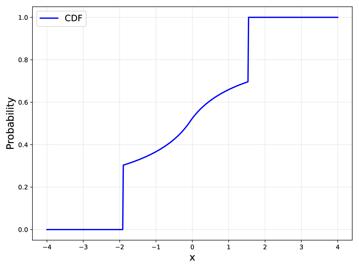
Figure 4. Cumulative distribution of $L^{0,1}_{\epsilon}$ for the Laplace mechanism with $\epsilon_{0}=1.0$ and $\epsilon=0.1$.

Appendix D Proof of Theorem 5

Proof.

The proof of this theorem follows similar lines as the proof of Lemma 12 in (Balle et al., 2019).

Define random variables $Y_{1}^{b}\sim\mathcal{R}(x_{1}^{b})$ and $W_{i}\sim\mathcal{R}(x_{2}),i=1,2,\dots,n-1$. $\mathbf{W}_{n-1}=\{W_{1},W_{2},\dots,W_{n-1}\}$. Let $\vec{y}\in\mathbb{Y}^{n}$ be a tuple of elements from $\mathbb{Y}$ and $Y\in\mathbb{N}_{n}^{\mathbb{Y}}$ be the corresponding multiset of entries. Then we have

$$\mathbb{P}[\{Y_{1}^{b}\}\cup\mathbf{W}_{n-1}=Y]=\frac{1}{n!}\sum_{\sigma}\mathbb{P}\left[(Y_{1}^{b},W_{1},\ldots,W_{n-1})=\vec{y}_{\sigma}\right],$$

where $\sigma$ ranges over all permutations of $[n]$ and $\vec{y}_{\sigma}=(y_{\sigma(1)},\ldots,y_{\sigma(n)})$. We also have

$$\mathbb{P}\left[(Y_{1}^{b},W_{1},\ldots,W_{n-1})=\vec{y}_{\sigma}\right]=\mathcal{R}(x_{1}^{b})(y_{\sigma(1)})\prod_{i=2}^{n}\mathcal{R}(x_{2})(y_{\sigma(i)}).$$

Summing this expression over all permutations $\sigma$ and factoring out the product of the $\mathcal{R}(x_{2})$’s yields:

$$\frac{1}{n!}\sum_{\sigma}\mathcal{R}(x_{1}^{b})(y_{\sigma(1)})\mathcal{R}(x_{2})(y_{\sigma(2)})\cdots\mathcal{R}(x_{2})(y_{\sigma(n)})$$

$$=\left(\prod_{i=1}^{n}\mathcal{R}(x_{2})(y_{i})\right)\left(\frac{1}{n}\sum_{i=1}^{n}\frac{\mathcal{R}(x_{1}^{b})(y_{i})}{\mathcal{R}(x_{2})(y_{i})}\right)$$

$$=\mathbb{P}[\mathbf{W}_{n}=Y]\cdot\frac{1}{n}\sum_{i=1}^{n}\frac{\mathcal{R}(x_{1}^{b})(y_{i})}{\mathcal{R}(x_{2})(y_{i})}.$$

Now we can plug these observation into the definition of $\mathcal{D}_{e^{\varepsilon}}$ and complete the proof as

$$D_{e^{\varepsilon}}\big{(}\mathcal{M}_{S}(X^{0}),\mathcal{M}_{S}(X^{1})\big{)}$$

$$=D_{e^{\varepsilon}}(\{Y_{1}^{0}\}\cup W_{n-1}\parallel\{Y_{1}^{1}\}\cup W_{n-1})$$

$$=\int_{\mathbb{N}_{n}^{\mathbb{Y}}}\left[\mathbb{P}[\{Y_{1}^{0}\}\cup W_{n-1}=Y]-e^{\varepsilon}\mathbb{P}[\{Y_{1}^{1}\}\cup W_{n-1}=Y]\right]_{+}$$

$$=\int_{\mathbb{N}_{n}^{\mathbb{Y}}}\mathbb{P}[W_{n}=Y]\left[\frac{1}{n}\sum_{i=1}^{n}\frac{\mathcal{R}(x_{1}^{0})(y_{i})-e^{\varepsilon}\mathcal{R}(x_{1}^{1})(y_{i})}{\mathcal{R}(x_{2})(y_{i})}\right]_{+}$$

$$=\mathbb{E}\left[\frac{1}{n}\sum_{i=1}^{n}\frac{\mathcal{R}(x_{1}^{0})(y_{i})-e^{\varepsilon}\mathcal{R}(x_{1}^{1})(y_{i})}{\mathcal{R}(x_{2})(y_{i})}\right]_{+}$$

$$=\mathbb{E}\left[\frac{1}{n}\sum_{i=1}^{n}G_{i}\right]_{+}.\qed$$

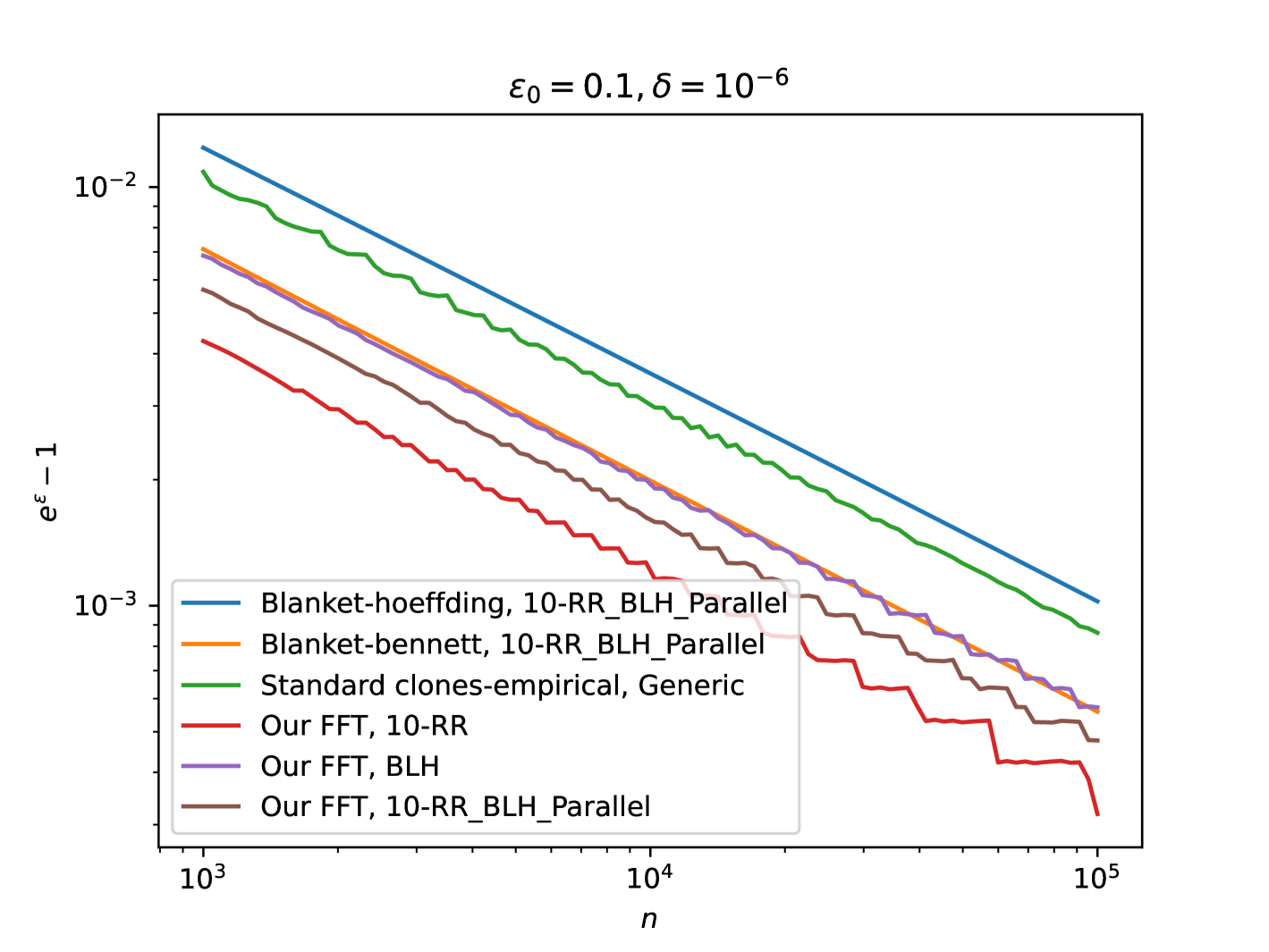
Figure 5. Parallel Composition, low $\epsilon_{0}$

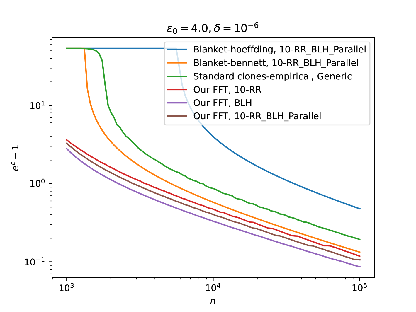
Figure 6. Parallel Composition, large $\epsilon_{0}$

Appendix E Experimental Results of Parallel Composition

We evaluate the parallel composition of 10-RR and BLH, where each mechanism is selected with equal probability $\boldsymbol{p}=[0.5,0.5]$. The experimental results (Figure 5 and 6) show that the amplification curve of the parallel composition lies between those of all individual components, aligning with theoretical expectations.

References

- (1)
- Acharya et al. (2019) Jayadev Acharya, Ziteng Sun, and Huanyu Zhang. 2019. Hadamard Response: Estimating Distributions Privately, Efficiently, and with Little Communication. In Proceedings of the Twenty-Second International Conference on Artificial Intelligence and Statistics (Proceedings of Machine Learning Research, Vol. 89), Kamalika Chaudhuri and Masashi Sugiyama (Eds.). PMLR, 1120–1129. https://proceedings.mlr.press/v89/acharya19a.html
- Apple and Google (2021) Apple and Google. 2021. Exposure Notification Privacy-preserving Analytics (ENPA) White Paper. https://covid19-static.cdn-apple.com/applications/covid19/current/static/contact-tracing/pdf/ENPA_White_Paper.pdf
- Balle et al. (2019) Borja Balle, James Bell, Adrià Gascón, and Kobbi Nissim. 2019. The Privacy Blanket of the Shuffle Model. In Advances in Cryptology – CRYPTO 2019: 39th Annual International Cryptology Conference, Santa Barbara, CA, USA, August 18–22, 2019, Proceedings, Part II (Santa Barbara, CA, USA). Springer-Verlag, Berlin, Heidelberg, 638–667. https://doi.org/10.1007/978-3-030-26951-7_22
- Balle et al. (2020) Borja Balle, Peter Kairouz, H. Brendan McMahan, Om Thakkar, and Abhradeep Thakurta. 2020. Privacy amplification via random check-ins. In Proceedings of the 34th International Conference on Neural Information Processing Systems (Vancouver, BC, Canada) (NIPS ’20). Curran Associates Inc., Red Hook, NY, USA, Article 388, 12 pages.
- Bassily et al. (2017) Raef Bassily, Kobbi Nissim, Uri Stemmer, and Abhradeep Thakurta. 2017. Practical locally private heavy hitters. In Proceedings of the 31st International Conference on Neural Information Processing Systems (Long Beach, California, USA) (NIPS’17). Curran Associates Inc., Red Hook, NY, USA, 2285–2293.
- Bassily and Smith (2015) Raef Bassily and Adam Smith. 2015. Local, Private, Efficient Protocols for Succinct Histograms. In Proceedings of the Forty-Seventh Annual ACM Symposium on Theory of Computing (Portland, Oregon, USA) (STOC ’15). Association for Computing Machinery, New York, NY, USA, 127–135. https://doi.org/10.1145/2746539.2746632
- Bittau et al. (2017) Andrea Bittau, Úlfar Erlingsson, Petros Maniatis, Ilya Mironov, Ananth Raghunathan, David Lie, Mitch Rudominer, Ushasree Kode, Julien Tinnes, and Bernhard Seefeld. 2017. Prochlo: Strong Privacy for Analytics in the Crowd. In Proceedings of the 26th Symposium on Operating Systems Principles (Shanghai, China) (SOSP ’17). Association for Computing Machinery, New York, NY, USA, 441–459. https://doi.org/10.1145/3132747.3132769
- Chen et al. (2024) E. Chen, Yang Cao, and Yifei Ge. 2024. A Generalized Shuffle Framework for Privacy Amplification: Strengthening Privacy Guarantees and Enhancing Utility. In Thirty-Eighth AAAI Conference on Artificial Intelligence, AAAI 2024, Thirty-Sixth Conference on Innovative Applications of Artificial Intelligence, IAAI 2024, Fourteenth Symposium on Educational Advances in Artificial Intelligence, EAAI 2014, February 20-27, 2024, Vancouver, Canada, Michael J. Wooldridge, Jennifer G. Dy, and Sriraam Natarajan (Eds.). AAAI Press, 11267–11275. https://doi.org/10.1609/AAAI.V38I10.29005
- Cheu et al. (2019) Albert Cheu, Adam Smith, Jonathan Ullman, David Zeber, and Maxim Zhilyaev. 2019. Distributed Differential Privacy via Shuffling. In Advances in Cryptology – EUROCRYPT 2019, Yuval Ishai and Vincent Rijmen (Eds.). Springer International Publishing, Cham, 375–403.
- Cheu and Zhilyaev (2022) Albert Cheu and Maxim Zhilyaev. 2022. Differentially Private Histograms in the Shuffle Model from Fake Users. 440–457. https://doi.org/10.1109/SP46214.2022.9833614
- Cormode et al. (2018a) Graham Cormode, Somesh Jha, Tejas Kulkarni, Ninghui Li, Divesh Srivastava, and Tianhao Wang. 2018a. Privacy at Scale: Local Differential Privacy in Practice. In Proceedings of the 2018 International Conference on Management of Data (Houston, TX, USA) (SIGMOD ’18). Association for Computing Machinery, New York, NY, USA, 1655–1658. https://doi.org/10.1145/3183713.3197390
- Cormode et al. (2018b) Graham Cormode, Tejas Kulkarni, and Divesh Srivastava. 2018b. Marginal Release Under Local Differential Privacy. In Proceedings of the 2018 International Conference on Management of Data (Houston, TX, USA) (SIGMOD ’18). Association for Computing Machinery, New York, NY, USA, 131–146. https://doi.org/10.1145/3183713.3196906
- Ding et al. (2017) Bolin Ding, Janardhan Kulkarni, and Sergey Yekhanin. 2017. Collecting telemetry data privately. In Proceedings of the 31st International Conference on Neural Information Processing Systems (Long Beach, California, USA) (NIPS’17). Curran Associates Inc., Red Hook, NY, USA, 3574–3583.
- Domingo-Ferrer and Soria-Comas (2022) Josep Domingo-Ferrer and Jordi Soria-Comas. 2022. Multi-Dimensional Randomized Response. In 2022 IEEE 38th International Conference on Data Engineering (ICDE). 1517–1518. https://doi.org/10.1109/ICDE53745.2022.00135
- Dwork (2006) Cynthia Dwork. 2006. Differential privacy. In Proceedings of the 33rd International Conference on Automata, Languages and Programming - Volume Part II (Venice, Italy) (ICALP’06). Springer-Verlag, Berlin, Heidelberg, 1–12. https://doi.org/10.1007/11787006_1
- Erlingsson et al. (2019) Úlfar Erlingsson, Vitaly Feldman, Ilya Mironov, Ananth Raghunathan, Kunal Talwar, and Abhradeep Thakurta. 2019. Amplification by shuffling: from local to central differential privacy via anonymity. In Proceedings of the Thirtieth Annual ACM-SIAM Symposium on Discrete Algorithms (San Diego, California) (SODA ’19). Society for Industrial and Applied Mathematics, USA, 2468–2479.
- Erlingsson et al. (2014) Úlfar Erlingsson, Vasyl Pihur, and Aleksandra Korolova. 2014. RAPPOR: Randomized Aggregatable Privacy-Preserving Ordinal Response. In Proceedings of the 2014 ACM SIGSAC Conference on Computer and Communications Security (Scottsdale, Arizona, USA) (CCS ’14). Association for Computing Machinery, New York, NY, USA, 1054–1067. https://doi.org/10.1145/2660267.2660348
- Feldman et al. (2022) Vitaly Feldman, Audra McMillan, and Kunal Talwar. 2022. Hiding Among the Clones: A Simple and Nearly Optimal Analysis of Privacy Amplification by Shuffling. In 2021 IEEE 62nd Annual Symposium on Foundations of Computer Science (FOCS). 954–964. https://doi.org/10.1109/FOCS52979.2021.00096
- Feldman et al. (2023a) Vitaly Feldman, Audra McMillan, and Kunal Talwar. 2023a. Stronger Privacy Amplification by Shuffling for Renyi and Approximate Differential Privacy. 4966–4981. https://doi.org/10.1137/1.9781611977554.ch181 arXiv:https://epubs.siam.org/doi/pdf/10.1137/1.9781611977554.ch181
- Feldman et al. (2023b) Vitaly Feldman, Audra McMillan, and Kunal Talwar. 2023b. Stronger Privacy Amplification by Shuffling for Rényi and Approximate Differential Privacy. arXiv:2208.04591 [cs.CR] https://arxiv.org/abs/2208.04591
- Imola et al. (2022) Jacob Imola, Takao Murakami, and Kamalika Chaudhuri. 2022. Differentially Private Triangle and 4-Cycle Counting in the Shuffle Model. In Proceedings of the 2022 ACM SIGSAC Conference on Computer and Communications Security (Los Angeles, CA, USA) (CCS ’22). Association for Computing Machinery, New York, NY, USA, 1505–1519. https://doi.org/10.1145/3548606.3560659
- Kairouz et al. (2017) Peter Kairouz, Sewoong Oh, and Pramod Viswanath. 2017. The Composition Theorem for Differential Privacy. IEEE Transactions on Information Theory 63, 6 (2017), 4037–4049. https://doi.org/10.1109/TIT.2017.2685505
- Kikuchi (2022) Hiroaki Kikuchi. 2022. Castell: Scalable Joint Probability Estimation of Multi-dimensional Data Randomized with Local Differential Privacy. arXiv:2212.01627 [cs.CR] https://arxiv.org/abs/2212.01627
- Koskela et al. (2021) Antti Koskela, Mikko A. Heikkilä, and Antti Honkela. 2021. Tight Accounting in the Shuffle Model of Differential Privacy. In NeurIPS 2021 Workshop Privacy in Machine Learning. https://openreview.net/forum?id=ZO6uneMKak0
- Koskela et al. (2020) Antti Koskela, Joonas Jälkö, and Antti Honkela. 2020. Computing Tight Differential Privacy Guarantees Using FFT. In Proceedings of the Twenty Third International Conference on Artificial Intelligence and Statistics (Proceedings of Machine Learning Research, Vol. 108), Silvia Chiappa and Roberto Calandra (Eds.). PMLR, 2560–2569. https://proceedings.mlr.press/v108/koskela20b.html
- Luo et al. (2022) Qiyao Luo, Yilei Wang, and Ke Yi. 2022. Frequency Estimation in the Shuffle Model with Almost a Single Message. In Proceedings of the 2022 ACM SIGSAC Conference on Computer and Communications Security (Los Angeles, CA, USA) (CCS ’22). Association for Computing Machinery, New York, NY, USA, 2219–2232. https://doi.org/10.1145/3548606.3560608
- Ren et al. (2018) Xuebin Ren, Chia-Mu Yu, Weiren Yu, Shusen Yang, Xinyu Yang, Julie A. McCann, and Philip S. Yu. 2018. LoPub : High-Dimensional Crowdsourced Data Publication With Local Differential Privacy. IEEE Transactions on Information Forensics and Security 13, 9 (2018), 2151–2166. https://doi.org/10.1109/TIFS.2018.2812146
- Team (2017) Apple Differential Privacy Team. 2017. Learning with privacy at scale. Apple Machine Learning Journal (2017).
- Wang et al. (2019b) Ning Wang, Xiaokui Xiao, Yin Yang, Jun Zhao, Siu Cheung Hui, Hyejin Shin, Junbum Shin, and Ge Yu. 2019b. Collecting and Analyzing Multidimensional Data with Local Differential Privacy . In 2019 IEEE 35th International Conference on Data Engineering (ICDE). IEEE Computer Society, Los Alamitos, CA, USA, 638–649. https://doi.org/10.1109/ICDE.2019.00063
- Wang et al. (2024) Shaowei Wang, Yun Peng, Jin Li, Zikai Wen, Zhipeng Li, Shiyu Yu, Di Wang, and Wei Yang. 2024. Privacy Amplification via Shuffling: Unified, Simplified, and Tightened. Proc. VLDB Endow. 17, 8 (April 2024), 1870–1883. https://doi.org/10.14778/3659437.3659444
- Wang et al. (2025) Shaowei Wang, Sufen Zeng, Jin Li, Shaozheng Huang, and Yuyang Chen. 2025. Shuffle Model of Differential Privacy: Numerical Composition for Federated Learning. Applied Sciences 15, 3 (2025). https://doi.org/10.3390/app15031595
- Wang et al. (2017) Tianhao Wang, Jeremiah Blocki, Ninghui Li, and Somesh Jha. 2017. Locally Differentially Private Protocols for Frequency Estimation. In 26th USENIX Security Symposium (USENIX Security 17). USENIX Association, Vancouver, BC, 729–745. https://www.usenix.org/conference/usenixsecurity17/technical-sessions/presentation/wang-tianhao
- Wang et al. (2020) Tianhao Wang, Bolin Ding, Min Xu, Zhicong Huang, Cheng Hong, Jingren Zhou, Ninghui Li, and Somesh Jha. 2020. Improving utility and security of the shuffler-based differential privacy. Proc. VLDB Endow. 13, 13 (Sept. 2020), 3545–3558. https://doi.org/10.14778/3424573.3424576
- Wang et al. (2019a) Tianhao Wang, Bolin Ding, Jingren Zhou, Cheng Hong, Zhicong Huang, Ninghui Li, and Somesh Jha. 2019a. Answering Multi-Dimensional Analytical Queries under Local Differential Privacy. In Proceedings of the 2019 International Conference on Management of Data (Amsterdam, Netherlands) (SIGMOD ’19). Association for Computing Machinery, New York, NY, USA, 159–176. https://doi.org/10.1145/3299869.3319891
- Wang et al. (2021) Tianhao Wang, Ninghui Li, and Somesh Jha. 2021. Locally Differentially Private Heavy Hitter Identification. IEEE Transactions on Dependable and Secure Computing 18, 2 (2021), 982–993. https://doi.org/10.1109/TDSC.2019.2927695
- Warner (1965) Stanley L. Warner. 1965. Randomized Response: A Survey Technique for Eliminating Evasive Answer Bias. J. Amer. Statist. Assoc. 60, 309 (1965), 63–69. http://www.jstor.org/stable/2283137
- Yang et al. (2024a) Mengmeng Yang, Taolin Guo, Tianqing Zhu, Ivan Tjuawinata, Jun Zhao, and Kwok-Yan Lam. 2024a. Local differential privacy and its applications: A comprehensive survey. Computer Standards & Interfaces 89 (2024), 103827. https://doi.org/10.1016/j.csi.2023.103827
- Yang et al. (2024b) Ruilin Yang, Hui Yang, Jiluan Fan, Changyu Dong, Yan Pang, Duncan S. Wong, and Shaowei Wang. 2024b. Personalized Differential Privacy in the Shuffle Model. In Artificial Intelligence Security and Privacy, Jaideep Vaidya, Moncef Gabbouj, and Jin Li (Eds.). Springer Nature Singapore, Singapore, 468–482.
- Ye and Barg (2017) Min Ye and Alexander Barg. 2017. Optimal schemes for discrete distribution estimation under local differential privacy. In 2017 IEEE International Symposium on Information Theory (ISIT). 759–763. https://doi.org/10.1109/ISIT.2017.8006630