On the Generalized Lambert Function
Abstract.
We consider a particular generalized Lambert function, , defined by the implicit equation , with and . Solutions to this equation can be found in terms of a certain continued exponential defined by formula (3.10). Asymptotic and structural properties of a non-trivial solution, , and its connection to the extinction probability of related branching processes are discussed. We demonstrate that this function constitutes a cumulative distribution function of a previously unknown non-negative absolutely continuous random variable.
Key words and phrases:
Continued exponential representation, Galton-Watson process, generalized Lambert function, iteration process, moment structure, Monte Carlo simulation, probability–generating function2020 Mathematics Subject Classification:
Primary 60E05, 60F05; Secondary 60E071. Introduction
The Lambert function has a long history going back to century. Nevertheless, it was rigorously introduced in 1996 only and studied relatively recently. This function is closely related to the logarithmic function and arises in many models of the different areas of sciences, including a number of problems in ecology and evolution theory. The main reason why the Lambert function became so popular is because this function allows us to solve explicitly important models for which this is not possible in terms of elementary functions.
The present paper is partly devoted to the interplays of the classical analysis, in particular, transcendental functions, probability theory as well as certain areas of computational mathematics, namely iteration schemes, Monte Carlo simulation and evolution of dynamical systems.
The classical Lambert function is defined as (the multi-valued) inverse function to
(see [8]) and therefore, it satisfies the following implicit equation:
This function was introduced by Lambert [17] in the second half of century and became a subject of Leonhard Euler’s studies [10] on the transcendental equations. Since then thousands of papers dedicated to the Lambert function and its generalizations were published.
The function , has many applications in various areas including mathematical and theoretical physics [8], [9], [18], [20]. This function is deeply connected to many explicitly solvable models and problems ranging from population growth rates to fertilization kinetics and disease dynamics [6], [18], [19], [20], [23], [24].
The function provides an exact solution to the equation
(see [8]). The function , the principal real branch of the Lambert function, has the Taylor series expansion
with the radius of convergence, . It also admits the following continued exponential representation [8]
| (1.1) |
Generalizations of the Lambert function were also relatively recently considered. In particular, in quantum mechanics research on Bose-Fermi statistics the equation
where and are particular polynomials of degrees and respectively, was analyzed [21]. In [6], [7] applications of the generalized Lambert functions are recently seen in the area of atomic, molecular, and optical physics.
In the theory of branching processes, a generalization of the Lambert equation describes the extinction probability of an explosive Galton-Watson branching process.
Probabilistic flavour of the solution to the generalized Lambert equation (see Section 2) naturally leads to an interesting family of random variables that we denote in what follows. The moments of can be computed in closed form. The study of the analytical properties of the moments lead to an elegant area of mathematics called Tornheim series (see [26] as well as [2], [3], [4], [5], [16]).
The structure of the present paper is as follows. In Section 2 we discuss connection between the generalized Lambert function and the extinction probability of the Galton-Watson process. In Section 3 the main analytical properties of the generalized Lambert functionare discussed.
In Section 4, we describe the asymptotic expansions and two-sided bounds for the generalized Lambert function. In Section 5, the numerical examples of the computation of the generalized Lambert function are discussed. A probabilistic interpretation of the generalized Lambert function and characteristics of the corresponding random variables are discussed in Section 6. Some technical statements are deferred to the Appendix.
To conclude the Introduction, we summarize some relevant notation and terminology. Hereinafter, , , , , , stand for the sets of all complex numbers, all real numbers, all positive reals, all integers, and all non-negative integers, respectively. In what follows, we use the notation for the cumulative distribution function (or cdf) of the random variable (r.v.) . The symbol “” stands for the survival function, . The notation “” is used for the moment of the random variable , . The natural logarithm of is denoted by . The Gamma function is traditionally denoted by , , . The Riemann zeta function is denoted by , . If is real and ,
2. Extinction probability of a Galton-Watson process
Extinction probability of a Galton-Watson process satisfies the equation
| (2.1) |
where is the probability generating function of the number of offsprings, , in the branching process (see [11], [13], [14]). If the r.v. has a Poisson distribution with parameter , then Equation (2.1) takes the form
and can be transformed to
The connection with the classical Lambert function and the Lambert equation becomes clear in this case.
If the distribution of the r.v. belongs to the class of discrete stable distributions the probabilities , are defined by the equation
where is a particular case of the Wright function, such that given , , argument with and real ,
| (2.2) |
A discrete stable r.v., , with parameters and is characterized by its p.g.f.,
| (2.3) |
The well-known case corresponds to the subclass of Poisson distributions which are naturally incorporated to the family of discrete stable laws.
The probability of ultimate extinction for a supercritical Galton-Watson process with discrete stable branching mechanism that starts from one particle appears to be intimately connected to a generalized Lambert function. Indeed, Equation (2.1) can be written as
Denote . Then and the latter equation can be written as follows:
| (2.4) |
where .
The following rather elementary assertion stipulates the existence and uniqueness of the solution to (2.4).
Proposition 2.1.
Let and . Then Equation (2.4) has the unique solution in the open interval .
Proof.
Indeed, consider the function
| (2.5) |
We have
The second derivative . Therefore, the function is convex in the interval and Equation (2.4) has a unique solution, , satisfying the inequalities . ∎
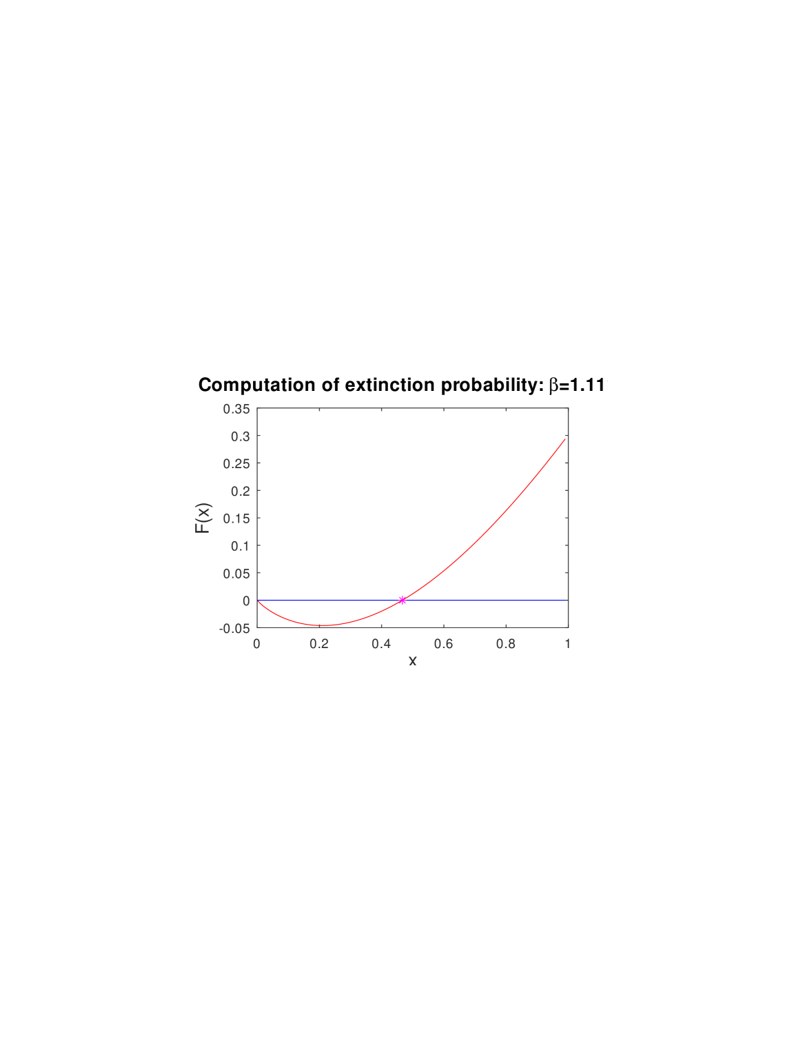
Here, the root of the equation is shown by the star in Figure 1. For and , the root . The root of Equation (2.4) is found by the iteration process described by Theorem 3.7 in the next Section. The iteration process is stopped once the iterations, , satisfy the inequality
where . For the above example, the number of iterations .
3. A generalized Lambert function
In this section we consider a formal definition and some analytical properties of the generalized Lambert function. Consider the function defined by the formula
| (3.1) |
where parameter is fixed.
Definition 3.1.
The inverse function to is called the generalized Lambert function.
We shall denote the generalized Lambert function by in what follows.
Since is analytic for and continuous at , one can see that is a real-valued, analytic function for . Both functions and are monotonically increasing. Indeed, the derivative of is equal to
Then we obtain that
Therefore, the generalized Lambert function is defined uniquely for any .
Remark 3.2.
From (3.1) it immediately follows that the function is represented by the absolutely convergent series
| (3.2) |
Since , the derivative
for . Note that blows up at for . For it is defined at by continuity.
Let . The generalized Lambert function obviously satisfies the following transcendental equation:
| (3.3) |
with and parameter .
Remark 3.3.
Remark 3.4.
Now, consider x as a fixed parameter and solve Equation (3.3) with respect to .
Lemma 3.5.
For each Equation (3.3) has two non-negative solutions, one of which is always 0, and the other one belongs to .
The function is intimately connected to the mapping, , defined by the relation
where
| (3.5) |
and . The mapping has a trivial fixed point:
Given , the non-trivial fixed point of represents the value of the function, , that is a solution of Equation (3.3).
The next statement describes the set of functions, and delineates the probabilistic nature of the set .
Let be the totality of all cumulative distribution functions of non-negative and absolutely continuous random variables.
Proposition 3.6.
For all we have
| (3.6) |
Proof.
We need to prove that
-
i.
The limits
(3.7) and
(3.8) -
ii.
The function is monotone.
-
iii.
The function is absolutely continuous.
Proof of i. From the definition of the inverse function, , we derive that the limits of the inverse function satisfy the relations
| (3.9) |
Proof of ii. Monotonicity of immediately follows from the inequality
Proof of iii. The last statement is obvious.
Thus, the set of functions, , is a subset of . ∎
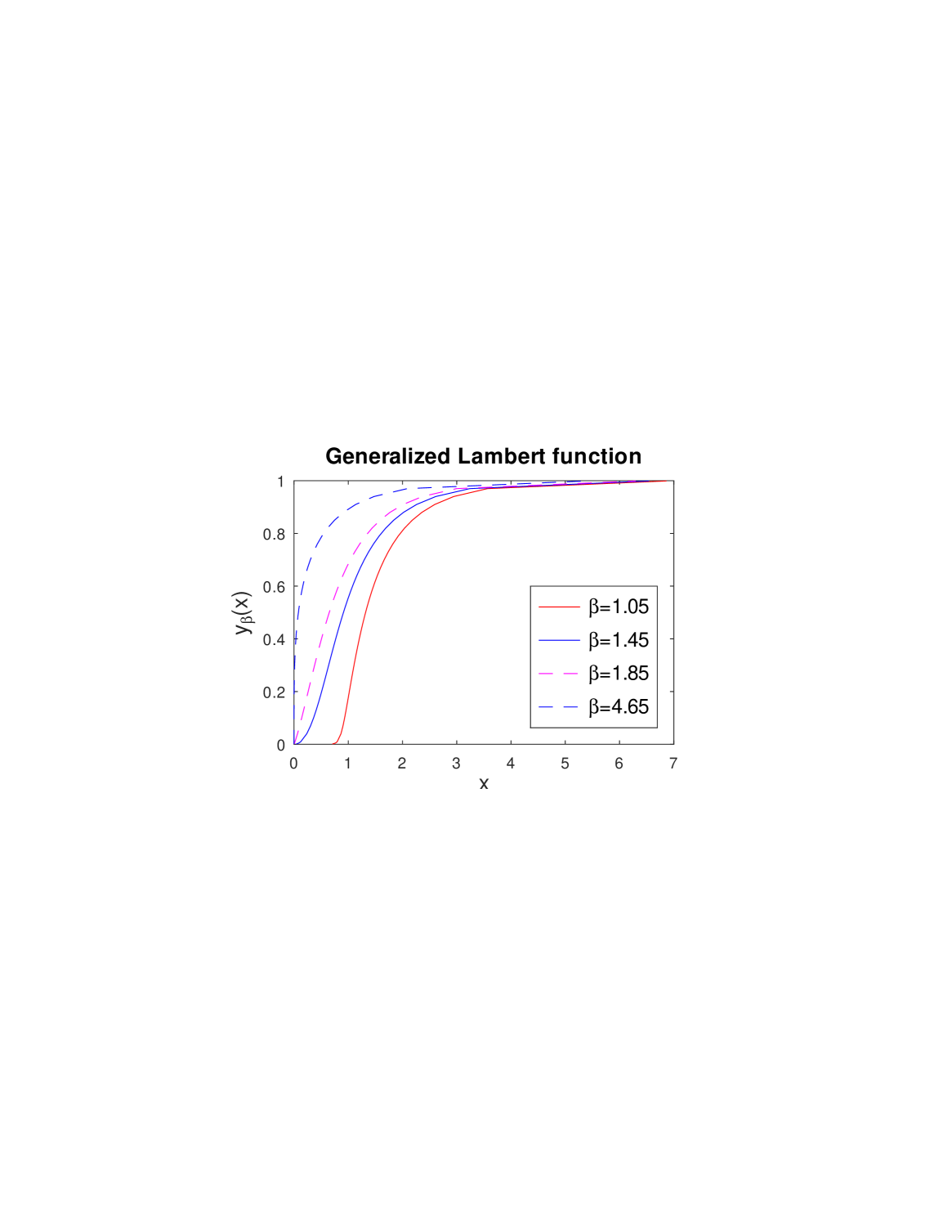
Let us now consider a useful computational scheme for the functions . The inverse function, , can be naturally used for the computation of for different values of the parameter , see Figure 2. More precisely, we take a finite set
for sufficiently large and compute the corresponding values of ,
Hereafter, we shall call the linear interpolation between the nodes , the benchmark approximation of the function .
Theorem 3.7.
Remark 3.8.
It is obvious that .
Lemma 3.9 (Monotonicity of ).
Consider the sequence defined by the relation with an arbitrary initial value, . Then we have
| (3.11) |
| (3.12) |
Moreover, if and the sequence is defined by the same mapping, , , then
Proof of Lemma.
The proof of the lemma follows immediately from the monotonicity of the function
that we obtain from the inequality for and . Suppose that . Let us prove that . But and . Since , we obtain that . Since , we derive that .
A similar reasoning allows us to conclude that if then , and we obtain that the inequality implies that for all integer .
The dual case, is analogous to the previous one: the latter inequality implies that for all integer .
The proof of the last statement of the Lemma is similar to the proof of the first statement. ∎
Next, denote
Lemma 3.10 (Contraction at fixed point).
-
i.
The fixed point, , of the mapping satisfies the relation
(3.13) -
ii.
The derivative, , diverges at :
-
iii.
The function is monotonically decreasing.
-
iv.
For , .
Proof of Lemma 3.10.
The function, , satisfies the relation
and
The latter inequality implies statement (iii).
Denote by the fixed point of the mapping . Then we have
Therefore,
Denote . Obviously, . Notice that for ,
Then we obtain that satisfies the inequality
Statement (i) is proved. Therefore, the function is a contraction near the fixed point , as was to be proved. The proof of statements (ii) and (iv) is straightforward. ∎
Proof of Theorem 3.7.
Fix and choose . It is not difficult to see that the sequence satisfies the inequality for if . Monotonicity and boundedness of the sequence implies that there exists the limit
This limit does not depend on the choice of because convergence to is monotone , and near the fixed point the mapping is a contraction. The limit, , satisfies (3.10) and we obtain that for all . Theorem 3.7 is thus proved. ∎
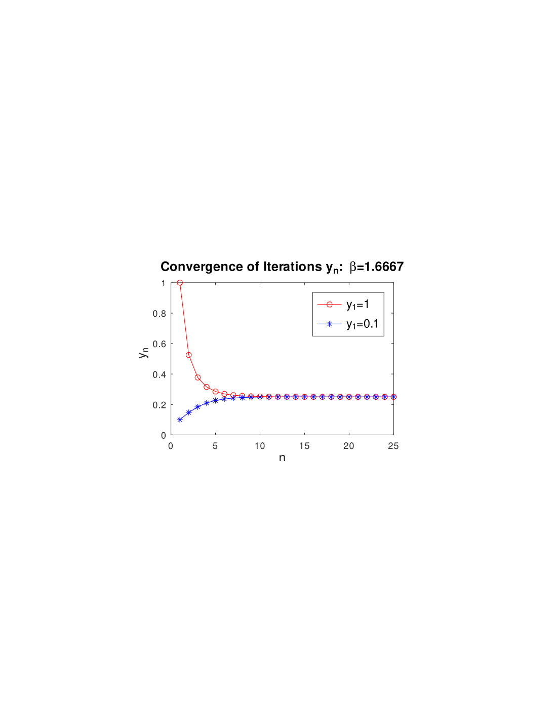
Convergence of iterations, , is illustrated in Figure 3. The integer parameter, , is the iteration index, the argument in Figure 3.
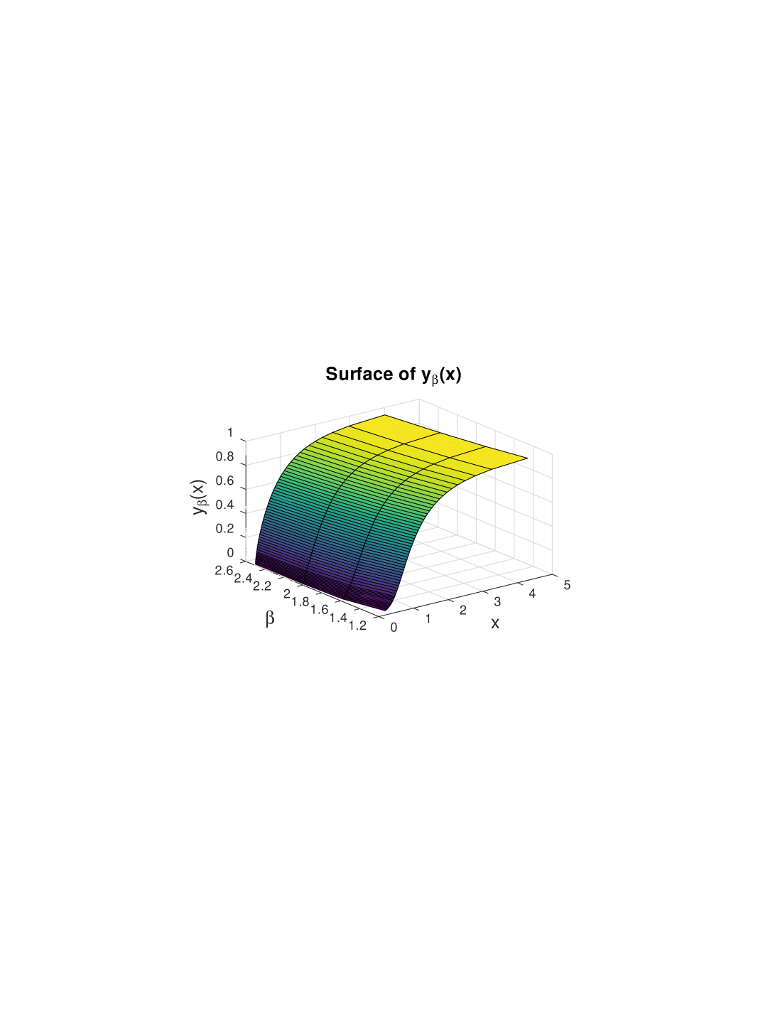
The values of the function, , also depend on the parameter, . If parameter is not fixed, we have a function of two arguments, .
Proposition 3.11.
The function is a monotone function of .
Proof.
Consider the inverse function corresponding to the function . From the definition of the inverse function (3.1) it follows that is monotonically decreasing function of the parameter . Then we immediately obtain that the inverse function to is monotonically increasing function of . Proposition 3.11 is thus proved. ∎
Since the limit of iterations, , does not depend on the initial value, , we obtain the following
Corollary 3.12.
For any the function admits the following continued exponential representation:
| (3.14) |
where .
4. Asymptotic behaviour of function .
In this section, we consider the asymptotic behaviour of for both small and large values of argument . First, we construct the following asymptotic expansion for function in the right-hand neighbourhood of .
Proposition 4.1.
The function, , has the following asymptotic on the lower tail:
| (4.1) |
Proof.
We have
Let us rewrite Equation (3.3) as
Then we obtain from the latter equation that
| (4.2) |
Let . Since , the parameter is positive and hence, we get for small that
From (4.2) and the latter asymptotic formula we obtain that satisfies the following relation:
Then we derive that
and, finally,
The proposition is thus proved. ∎
The asymptotics (4.1) of , as , is just a starting point. It can be improved as follows:
Proposition 4.2.
The function, admits the following asymptotic expansion as :
| (4.3) |
The proof of this proposition is deferred to the Appendix.
Corollary 4.3.
The function satisfies the following limit relation
Remark 4.4.
Let us introduce a new variable, and define
The function satisfies the following transcendental equation:
where
It is instructive to look at the graph of the function .
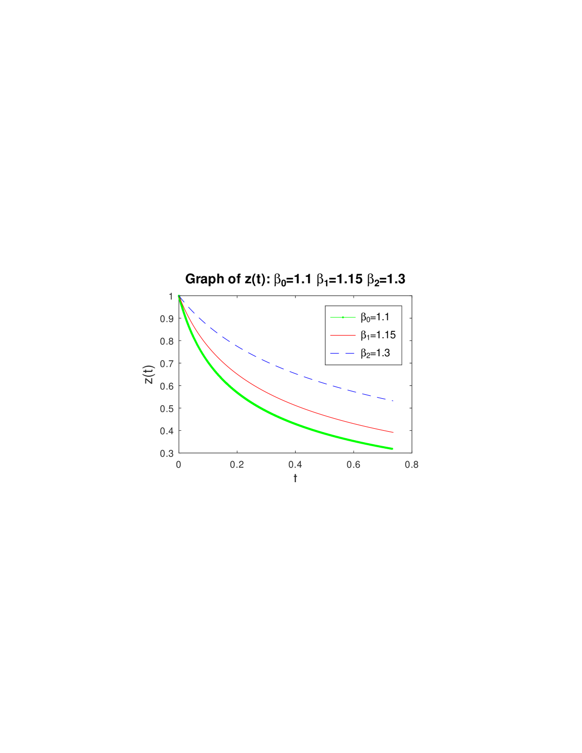
In Figure 5 the graph of the function is shown for the following three particular values of : , , . All three graphs, obviously, start at the point . The function is downward convex, positive and monotonically decreasing.
Conjecture
The function , , is analytical.
Our next step is the derivation of the two-sided bounds for the function . Numerical comparison of the approximations (4.1) and (4.3) and the lower bound, , introduced in Proposition 4.5, is discussed in Section 5.
Proposition 4.5.
For and , the function satisfies the following two-sided inequality:
| (4.4) |
Proof.
It follows from the definition of the inverse function that
Since , we have
The latter inequality can be written as
Therefore,
On the other hand, since
we obtain that
The latter inequality is equivalent to The upper bound, , and the lower bound, , hence established. ∎
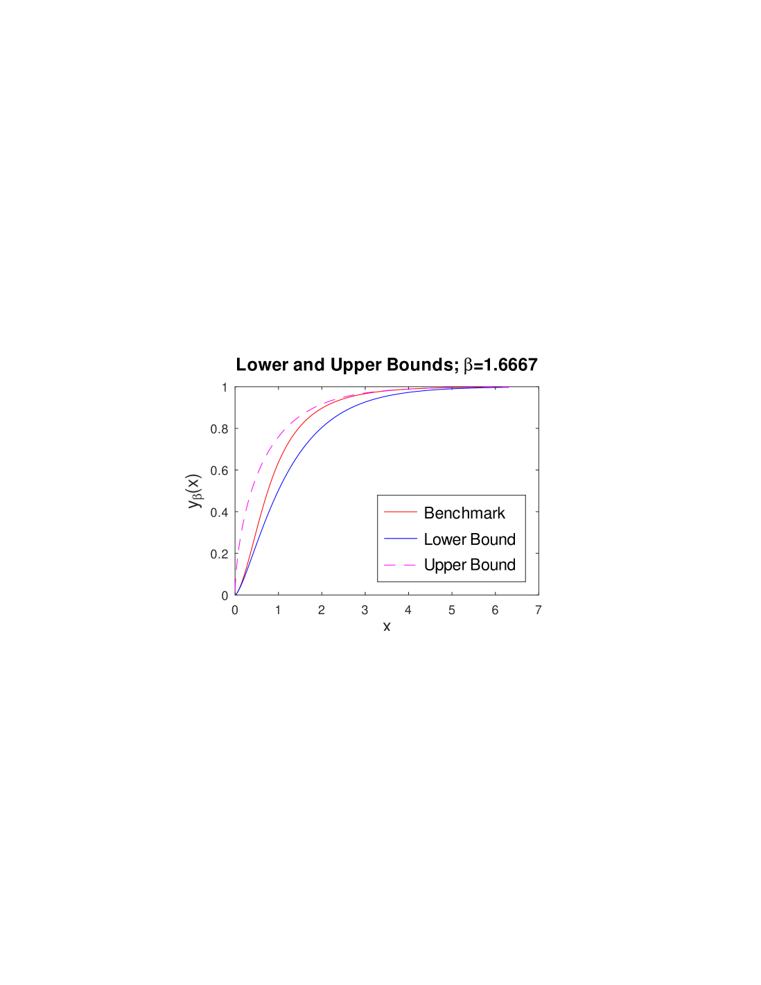
In Figure 6 the graph of the function, , is displayed together with the upper and lower bounds established in Proposition 4.5. The lower bound captures the asymptotic behaviour of the function as while the upper bound captures the asymptotic behaviour of as .
It is also not difficult to see that the ratio of the bounds approaches at infinity
| (4.5) |
Indeed, the ratio , can be written as
where The latter relation implies the validity of (4.5).
5. Numerical examples
5.1. Roots of Equation (2.4)
The problem of the computation of the extinction probability can be addressed by using several numerical methods.
The first approach is related to solution of Equation (2.4), considered in Section 2, by bisection method. An important technical issue is due to the fact for the values of parameter close to this method often presents a difficulty in finding the interval containing the root of the equation. This situation is illustrated in Figure 7 where the graph of the function, , satisfying Equation (2.5), is shown for three different values of parameter : , and .
The positive root of the equation, marked by the star in Figure 7 is moving towards as .
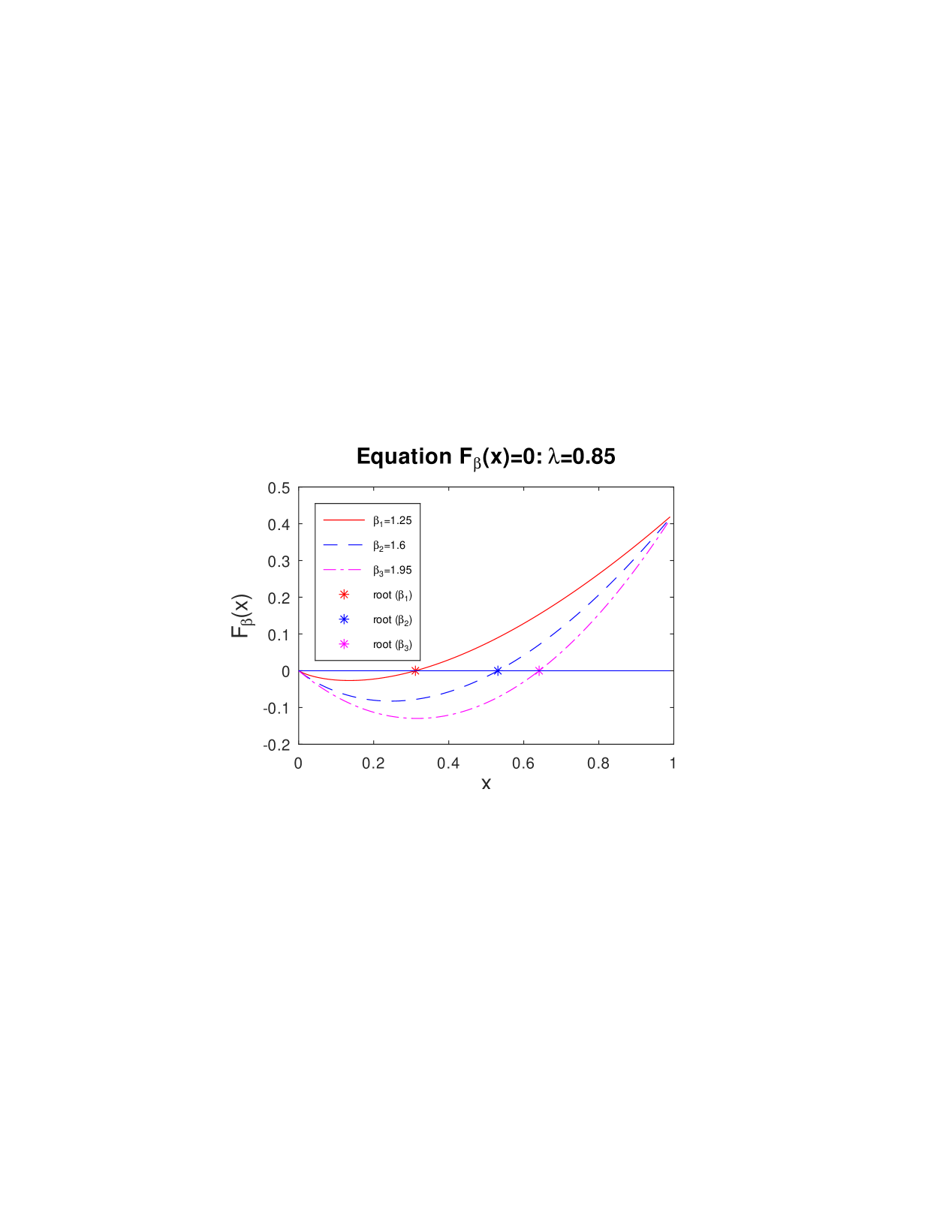
Moreover, the minimal value of the function tends to monotonically, namely, as . For this reason, the root of the equation, , as . Such a behaviour represents certain computational difficulties for the bisection method. The numerical experiments with MatLab demonstrate that the interval, , such that , remains undetermined for , due to computer finite precision.
5.2. Comparison of approximations
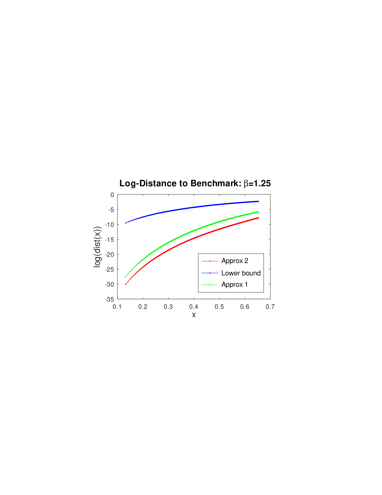
A much more efficient solution can be obtained by using the asymptotic approximations, derived in Section 4. Recall that the lower bound used as the asymptotic approximation of the function, , is .
The first and the second approximations, and of the function , defined by Equations (4.1) and (4.3), respectively, and the lower bound, , are compared with the benchmark approximation of . The methodology of comparison is founded on a fixed set, , of values of function, where are close to . Given , we compute the benchmark approximation, , , and the distances , , and for each .
In Figure 8 we compare logarithms of the distances, , and . Parameter . The set is an arithmetic progression,
where , , . The results shown in Figure 8 demonstrate advantage of the approximation .
Similar results are obtained for the other values of parameter , see Figure 9. In that Figure, parameter takes two values, and .
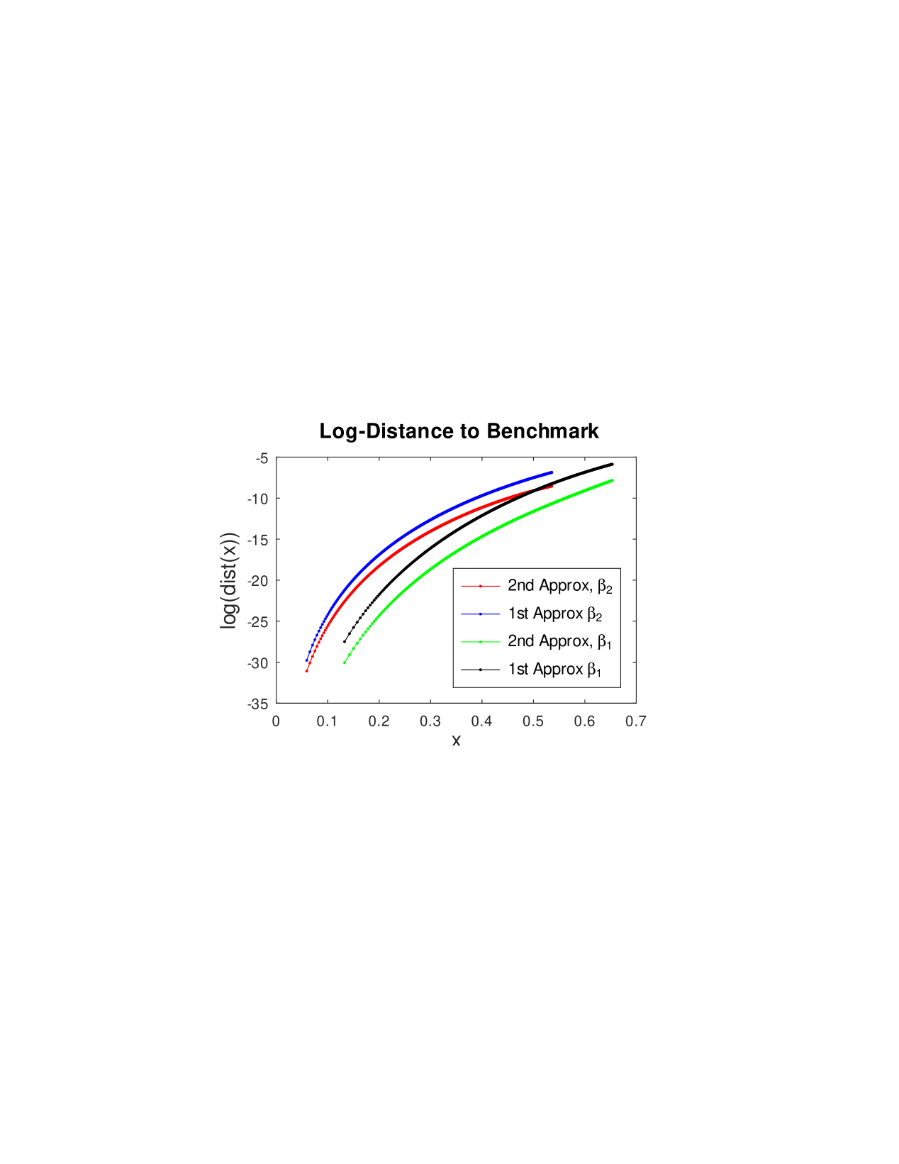
In both cases the numerical results demonstrate advantage of approximation (4.3).
5.3. The number of iterations required
The iterations described in Theorem 3.7 converge independently of the choice of the initial approximation, . However, the number of iterations, , required for a specified accuracy , does depend on as well as on and . Let us define more precisely.
Definition 5.1.
Given , the required number of iterations, , is defined as follows:
Let us compare the following strategies for the choice of :
-
1.
for all .
-
2.
.
-
3.
.
The first strategy always takes the initial approximation to coincide with the upper bound. The second strategy takes the initial approximation to be equal to the lower bound for the solution. The third strategy takes the mid-point as the initial approximation.
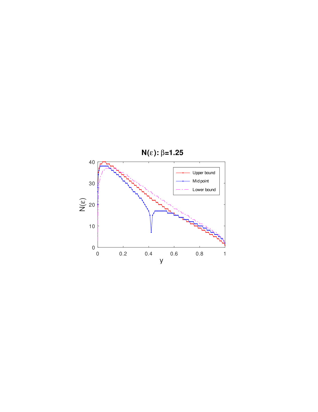
In Figure 10, the above three strategies are compared for . Parameter in the numerical experiment related to Figure 10 is described in this section.
It is convenient to change the argument in the definition of the required number of iterations to . In this case, the second argument of the function will belong to the interval .
While the argument is small enough, , the initial approximation, , dominates the other strategies. In the mid-range case, , the mid-point strategy, , provides a faster convergence than the remaining two strategies.
For the large values of the argument , such that , where , the first strategy is the most efficient. This fact is consistent with the property of the upper bound, , to provide the asymptotic approximation of as .
6. Definition and properties of the random variable
In the previous section we demonstrated that for each the function is the cdf of an absolutely continuous random variable denoted by . Despite the fact that the cdf of is not known explicitly, many characteristics of can still be found in closed form. In the next subsection, we compute the moments of this random variable.
6.1. Computation of the moments, .
Definition 6.1.
We say that the random variable has the generalized Lambert distribution if
Proposition 6.2.
The th moment of the r.v. is
| (6.1) |
where .
Proof.
Let be defined on a certain probability space and let be a random variable on the same probability space, , having uniform distribution. The random variable can be written as follows:
| (6.2) |
Then we obtain from (6.2) that the moments of the r.v. satisfy the relation
Changing the variables in the above integral ascertains the validity of (6.1). ∎
In Figure 11 the first 6 log-moments, of the random variable are shown for . The theoretical results are obtained from (6.1). These results are
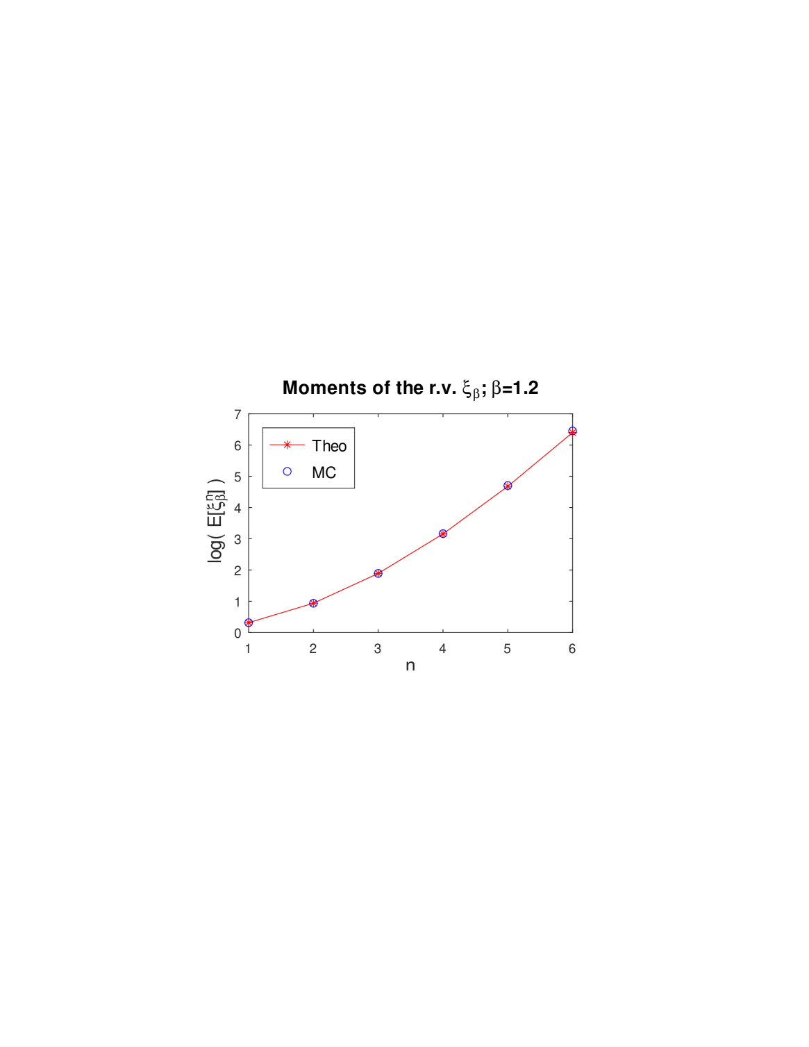
compared with that obtained by Monte Carlo method.
The following statement stipulates integrability of the function and demonstrates unexpected connection to the Riemann zeta function, .
Proposition 6.3.
The function satisfies the following relation:
| (6.3) |
Proof.
Obviously, we can write the first moment of as .
Proposition 6.4.
The second moment of the random variable, , satisfies the relation
| (6.5) |
The standard deviation of is
| (6.6) |
Proof.
In Figure 12, the first moment, and the standard deviation, are shown for . The analytical results are accompanied by the Monte Carlo valuation of the first moment of and the standard deviation of this random variable.
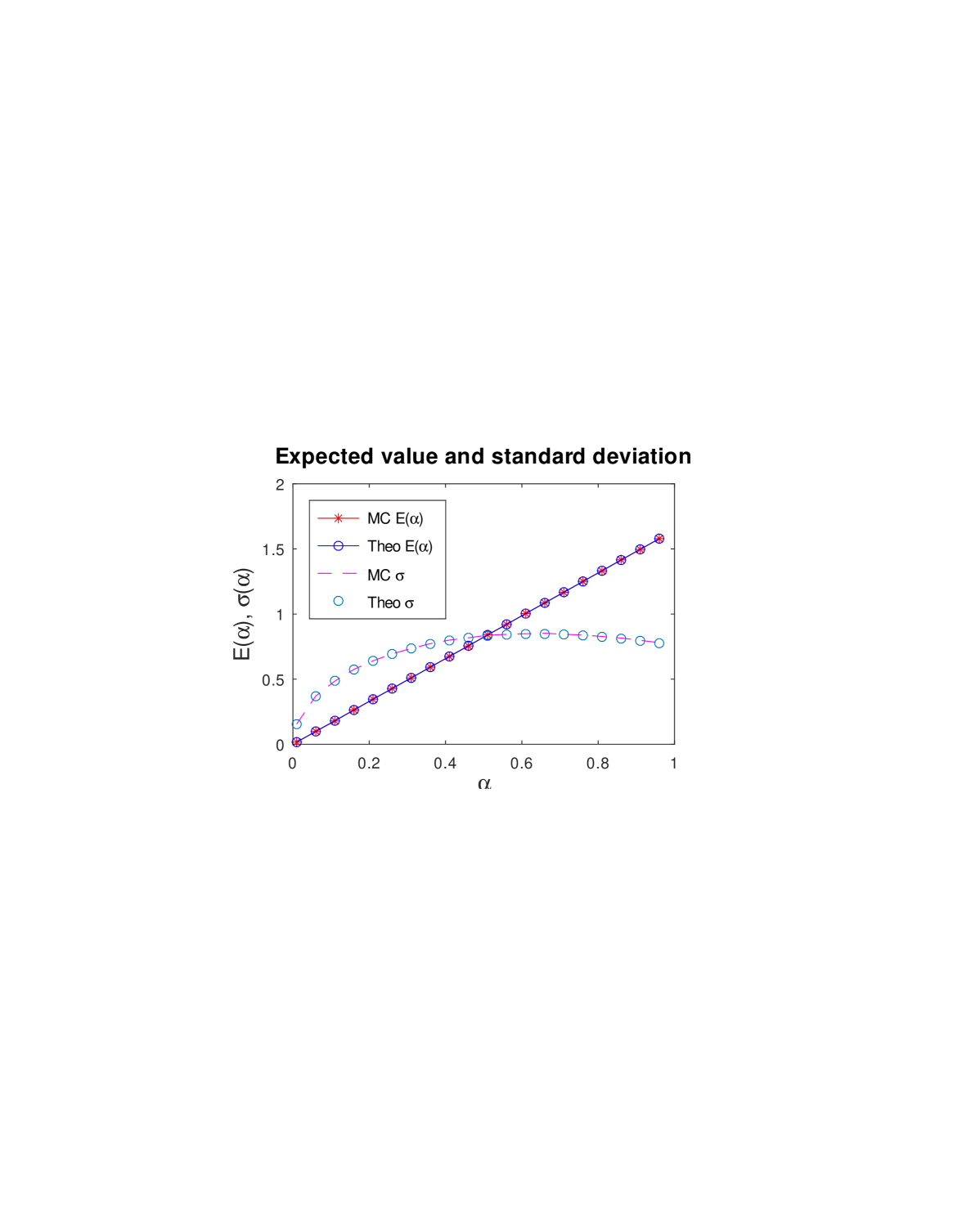
The theoretical value of the expectation, , and its MC estimator form a straight line in Figure 12. The standard deviation, , and its MC estimator exhibit a non-linear, non-monotone dependency on .
6.2. The moment problem for .
The classical moment problem [1], [15], [22], deals with existence and uniqueness of a finite, non-negative measure on such that a given sequence of real numbers, , , , , satisfying the relation
In this Section, we consider the case of the probability measure corresponding to the distribution of the random variable :
In this case, the support of the measure is .
Existence of such probability measure is obvious in our case. The uniqueness problem can be formulated as follows:
-
Given a sequence of moments, , is there another measure, , different from the probability measure defined by the cumulative distribution function , such that the th moment corresponding to measure is for all integer ?
If the solution to the moment problem is unique, we say that the moment problem is determinate. Otherwise the moment problem is said to be indeterminate.
Proposition 6.5.
Let the moments, , be defined by Equation (6.1):
Then there exists a unique probability measure, , on such that
The proof of Proposition 6.5 is based on the following technical statement on the rate of growth of the moments, .
Lemma 6.6.
The sequence exhibits the following asymptotic relation:
| (6.7) |
where the constant satisfies the inequalities
Proof of Lemma 6.6 is deferred to the Appendix.
Proof of Proposition 6.5.
Let us prove that the measure is determinate. We would like to verify the following sufficient condition for the moments of the probability measure concentrated on (see [15], [22], [25] ):
| (6.8) |
From (6.7) we derive that as
Then we find that
The latter asymptotic equation implies (6.8), as was to be proved.∎
6.3. Moments, generating function and identities
We conclude this section with a few remarks on the connection between the moments of the r.v. and the generating functions of several remarkable sequences including the sequence , where is the Riemann zeta function.
Proposition 6.8.
The integral, , satisfies the relation
| (6.10) |
Proposition 6.8 is proved in the Appendix.
Let us now represent the integral, , as the generating function of a harmonic sequence. Denote by , the sum of the harmonic series
and for we define . Obviously, we have
Let us now define the sequence
| (6.11) |
Proposition 6.9.
The elements of the sequence satisfy the relation
| (6.12) |
The integral is the generating function of the sequence :
| (6.13) |
The proof of Proposition 6.9 is deferred to the Appendix.
The double sums similar to (6.12) are usually called Tornheim series or Tornheim double sums. They find applications in many areas of mathematics and physics, see [16], [26].
Remark 6.10.
The sequence can also be expressed in terms of the Riemann zeta function as follows
The coefficient, , determines the asymptotic behaviour of the second moment as .
Proposition 6.11.
| (6.14) |
The proof of this proposition is deferred to the Appendix.
Corollary 6.12.
The variance of the r.v. admits the following asymptotics as :
Computation of the coefficients, , , …, requires computation of the harmonic sums
Corollary 6.13 (compare with [2], [12]).
-
i.
The coefficient satisfies the relation
-
ii.
The harmonic sum
Numerous representations of such character for harmonic sums can also be found in [12].
Analysis of the higher moments of leads to relations generalizing properties of harmonic double sums. This line of research will be considered in our subsequent work.
Acknowledgment. VVV appreciates hospitality of the Fields Institute and York University.
References
- [1] N. I. Ahiezer. The classical moment problem and some related questions in analysis. SIAM, Philadelphia, 2021.
- [2] I.A. Aliev and A. Dil. Tornheim-like series, harmonic numbers, and zeta values. Journal of Integer Sequences, 25, 2022. Article 22.5.5.
- [3] D. H. Bailey and J. M. Borwein. Computation and experimental evaluation of Mordell–Tornheim–Witten sum derivatives. Exp. Math., 27:370–376, 2018.
- [4] D. Borwein and J.M. Borwein. On an intriguing integral and some series related to . Proc. Amer. Math. Soc., 123:1191–1198, 1995.
- [5] J. M. Borwein. Hilbert’s inequality and Witten’s zeta-function. Amer. Math. Monthly, 115:125–137, 2008.
- [6] A. Braun, A. Wokaun, and H. Hermanns. Analytical solution to a growth problem with two moving boundaries. Appl. Math. Model, 27:47–52, 2003.
- [7] P. Castle. Taylor series for generalized Lambert functions, 2018.
- [8] R. M. Corless, G. H. Gonnet, D. E. G. Hare, D. J. Jeffrey, and D. E. Knuth. On the Lambert function. Advances in Computational Mathematics, 5:329–359, 1996. doi:10.1007/BF02124750. S2CID 29028411.
- [9] D. Daley and J. Gani. Epidemic Modelling: An Introduction. Cambridge University Press, 2005.
- [10] L. Euler. De serie lambertina plurimisque eius insignibus proprietatibus. Acta Acad. Scient. Petropol, 2:29–51, 1783.
- [11] W. Feller. An Introduction to Probability Theory and Its Applications, volume 2. Wiley, New York, 1968.
- [12] P. Flajolet and B. Salvy. Euler sums and contour integral representations. Experimental Mathematics, 7(1):15–35, 1998.
- [13] S. Karlin and H. M. Taylor. A First Course in Stochastic Processes. Academic Press, New York, 1975.
- [14] A.N. Kolmogorov and N.A. Dmitriev. Branching random processes. Soviet Mathematics. Doklady, 56(1):7–10, 1947. (in Russian). English translation in: Shiryayev, A.N. (ed.), Selected Works of A.N. Kolmogorov, 2, 309–314, Kluwer, Dordrecht.
- [15] M.G. Krein and A.A. Nudelman. The Markov moment problem and extremal problems, volume 50. Providence, 1977. Translations of Mathematical Monographs AMS.
- [16] M. Kuba. On evaluations of infinite double sums and Tornheim’s double series, 2008.
- [17] J. H. Lambert. Observationes variae in mathesin puram. Acta Helveticae, physico-mathematico-anatomico-botanico-medica, Band III:128–168, 1758.
- [18] J. Lehtonen. The Lambert function in ecological and evolutionary models. Methods in Ecology and Evolution, 7:1110–1118, 2016. doi:10.1111/2041-210x.12568, S2CID 124111881.
- [19] A. Maignan and T. C. Scott. Fleshing out the generalized Lambert function. ACM Commun. Comput. Algebra, 50:45–60, 2016.
- [20] I. Mezö. The Lambert Function: Its Generalizations and Applications. Discrete Mathematics and its applications. CRC Press, Boca Raton, FL, 2022. doi:10.1201/9781003168102.
- [21] I. Mezö and A. Baricz. On the generalization of the Lambert function with applications in theoretical physics, 2015.
- [22] K. Schmüdgen. Ten lectures on the moment problem, 2020. arXiv.2008.12698.
- [23] T. C. Scott, R. B. Mann, and R. E. Martinez. General relativity and quantum mechanics: Towards a generalization of the Lambert function. AAECC (Applicable Algebra in Engineering, Communication and Computing), 17(1):41–47, 2006. arXiv:math-ph/0607011.
- [24] T.C. Scott, J.F. Babb, A. Dalgarno, and J. D. Morgan. The calculation of exchange forces: General results and specific models. J. Chem. Phys., 99:2841–2854, 1993. doi:10.1063/1.465193. ISSN 0021-9606.
- [25] A. N. Shiryaev. Probability, volume 1. Springer, New York, 2016.
- [26] L. Tornheim. Harmonic double series. Amer. J. Math., 72:303–314, 1950.
Appendix A Proof of Technical Results
Proof of Proposition 4.2.
Let us represent the function, , as
| (A.1) |
Then, obviously,
From Equation (4.1) it follows that the limit
It is convenient to introduce the variable . Denote by . Then we obtain that the function satisfies the implicit equation
| (A.2) |
Let us represent the function in the following form:
| (A.3) |
Then substituting (A.3) into (A.2), we recursively derive the first coefficients in Expansion (A.3):
The proposition is thus proved. ∎
Proof of Lemma 6.6.
We have to prove that the moments have the following asymptotics:
where the constant satisfies the inequality Since the support of the measure is , the moment, , can be evaluated as follows:
where the survival function . Therefore,
| (A.4) |
where . Combining (4.4) and (A.4) we derive the inequalities
| (A.5) |
Next, consider the integral
Taking into account that
as , we obtain the following asymptotic relation as
| (A.6) |
where is the Gamma function. Then from (A.5) and (A.6) we obtain that
The lemma is thus proved. ∎
Proof of Proposition 6.8.
Recall the representation of the function by the following convergent series:
Hence, the integral can be written as follows:
The latter relation implies that
The proposition is thus proved. ∎
Proof of Proposition 6.9.
Consider the double sum in (6.10). We have that for ,
Then we derive that
The latter relation implies (6.12). Now, consider the inner double sum,
Changing the summation index, , we obtain that
It is obvious that the latter sum is equal to . Therefore,
From the definition of the sequence (see Equation (6.11)) we obtain that
as was to be proved. ∎