BRT: Boundary representation learning via Transformer

Abstract

The recent rise of generative artificial intelligence (AI), powered by Transformer networks, has achieved remarkable success in natural language processing, computer vision, and graphics. However, the application of Transformers in computer-aided design (CAD), particularly for processing boundary representation (B-rep) models, remains largely unexplored. To bridge this gap and align CAD with the AI trend, this paper introduces Boundary Representation Transformer (BRT), a novel method adapting Transformer for B-rep learning. B-rep models pose unique challenges due to their irregular topology and continuous geometric definitions, which are fundamentally different from the structured and discrete data Transformers are designed for. To address this, BRT proposes a continuous geometric embedding method that encodes B-rep surfaces (trimmed and untrimmed) into Bézier triangles, preserving their shape and continuity without discretization. Additionally, BRT employs a topology-aware embedding method that organizes these geometric embeddings into a sequence of discrete tokens suitable for Transformers, capturing both geometric and topological characteristics within B-rep models. This enables the Transformer’s attention mechanism to effectively learn shape patterns and contextual semantics of boundary elements in a B-rep model. Extensive experiments demonstrate that BRT achieves state-of-the-art performance in part classification and feature recognition tasks.

1 Introduction

Extracting semantic information from computer-aided design (CAD) models via deep learning is a critical step toward developing next-generation intelligent CAD systems [1, 2]. CAD models are typically represented by the boundary representation (B-rep) scheme—a hierarchical collection of boundary elements of vertices, edges, loops, faces, and shells [3]—due to its wide application in part/assembly design [4, 5], engineering analysis [6], and process planning [7]. Their irregular topology (i.e., connectivity among boundary elements) and continuous geometric definitions (i.e., curves and surfaces) pose unique challenges distinct from the structured formats for which most deep neural networks are designed, such as sequences (1D text) or grids (2D images).

A common approach to addressing these challenges involves converting B-rep models into intermediate representations, such as point clouds, voxels, or multi-view images, to allow direct application of existing deep networks [8, 9, 10, 11, 12, 13]. However, these methods often compromise topological information [14], which is critical for preserving the integrity of B-rep models and supporting downstream applications like parametric design [15, 16], FEM analysis  and tool path generation [17, 18]. Recent efforts have turned to graph neural networks (GNNs) to explicitly process topological information [19, 1, 20, 21, 22]. Despite the improved performance, these methods still rely on converting continuous geometric data into discrete forms. No universal discretization parameters suit all cases and consequently, tedious manual tuning is required, limiting these methods’ applicability.

Recently, Transformer networks have emerged as the dominant architecture in natural language processing, computer vision, and computer graphics [23, 24, 25]. There are good reasons to extend Transformers to the CAD domain, particularly for B-rep models. First, Transformers serve as the backbone of the recent generative AI technologies, such as ChatGPT [26]. Adapting Transformers for B-rep learning allows the CAD domain to stay aligned with this AI trend. Second, the attention mechanism of Transformer networks excels at capturing complex relationships within input data, and this makes them particularly well-suited for modeling the intricate topological patterns and geometric similarities within B-rep models [27], which are challenging to handle with traditional neural networks like GNNs.

This paper presents an approach, called Boundary Representation Transformer (BRT), for learning B-rep models using Transformers. Unlike languages or images, which exhibit regular structures, B-rep models are characterized by their irregular topology [28]. Moreover, while languages and images are inherently discrete in their content, B-rep models are continuous in their geometry (e.g., B-spline curves and surfaces [29]). Consequently, extending Transformers originally designed for sequential and discrete data to B-rep models is no trivial matter. The fundamental challenge here is transforming irregular, continuous B-rep models into a sequence of structured tokens that Transformers can effectively process. (A token is a small, meaningful unit of raw data that AI models can understand, for example, a word [24].)

To effectively tokenize B-rep models, BRT introduces a novel geometric embedding method that maps each boundary element into a high-dimensional vector space, where the vector captures the geometric characteristics of the boundary element. Unlike existing approaches, this method operates completely in the continuous domain, eliminating the need for any discretization. This is achieved by decomposing a surface (trimmed or untrimmed) into a collection of Bézier triangles while preserving the surface shape. Bézier triangles are advantageous because they are continuous, offer greater flexibility in shape representation, and most importantly, have a regular structure—always having a fixed number of control points for a given degree [30].

After obtaining the geometric embeddings, BRT further applies a topology-aware embedding method to organize all the geometric embeddings into face-based tokens for input into Transformers. It leverages the hierarchical relationships (e.g., vertex-edge relationships), cyclic relationships (e.g., edge-loop relationships), and parallel relationships (e.g., face-face adjacency relationships) among the boundary elements to guide the organization. As such, the resulting tokens capture not only the geometric characteristics but also the topological patterns of the boundary elements within B-rep models. This enables more comprehensive and context-aware tokenization of B-rep models compared to existing methods. As a result, it can provide a solid foundation for Transformers to learn meaningful representations that capture the semantics within B-rep models.

The main contributions of this paper are as follows:

1. A novel method that adapts the most advanced Transformer networks in deep learning for processing B-rep models in CAD. To the best of our knowledge, this is the first approach to integrate these two aspects.

2. A continuous geometric embedding method that learns geometric features from B-rep models without the need for discretization into points, meshes, or voxels, unlike existing methods.

3. A topology-aware embedding method for more comprehensive and context-sensitive tokenization of B-rep models compared to existing approaches.

The remainder of this paper is organized as follows. Sec. 2 reviews the literature, Secs. 3 elaborate the methods of BRT. Validation of the method using a series of examples and comparisons can be found in Sec. 4, followed by conclusions in Sec. 5.

2 Related Work

With rapid advancements in deep learning, 3D geometric modeling is shifting from traditional rule-based methods to data-driven approaches [31]. B-rep modeling follows this trend, with development broadly falling into two categories: conversion-based and direct methods. The former converts B-rep models into intermediate representations, such as point clouds, voxels, or multi-view images, allowing the direct use of existing deep learning networks from computer vision and graphics. The latter focuses on directly modeling the topological aspects of B-rep models using neural networks like GNNs. The following summarizes these two lines of research, as well as the application of Transformer networks to 3D modeling, which is closely related to this work.

Conversion-Based Methods. Effective learning algorithms have been developed for discrete 3D models such as point clouds, meshes, and voxels. Notable examples include PointNet/PointNet++ [32, 8] and Dynamic Graph CNN [33] for point clouds, MeshCNN [34], MeshNet [35], and MeshWalker [36] for meshes, and O-CNN [37] for voxels, among others. Recent works in these areas (e.g., [38, 39, 40, 41, 42]) have further advanced the state of the art. In this regard, a natural choice for handling B-rep models is to convert them into these discrete representations, as demonstrated by methods like FeatureNet [10], Mesh-Faster RCNN [43], and ASIN [9]. In addition to 3D discrete representations, some approaches convert 3D objects to 2D views, allowing traditional 2D CNNs to be applied directly [44, 45, 13]. While these conversion-based methods have been effective in certain applications, they compromise topological information (i.e., connectivity among boundary elements), which is crucial for maintaining the integrity of B-rep models and supporting downstream tasks, limiting their overall applicability.

Direct Methods. These methods aim to directly learn from B-rep models without relying on intermediate representations. While presented in various forms, common to them is the use of GNNs to process the model’s topology [46, 19, 47, 1, 20, 21, 22]. This concept was first introduced by Cao et al. [46], although their work was restricted to planar surfaces. Subsequent advancements expanded this approach to quadratic and freeform surfaces, as seen in UV-Net [19] and Hierarchical CADNet [1]. These methods discretize surfaces into point clouds or meshes and use existing learning algorithms (e.g., CNNs) to encode them as GNN nodes. In addition to discretization, heuristic descriptors (such as face type, face genus, and face-face concavity/convexity) have also been employed to encode faces for use as GNN nodes, e.g., BRepGAT [20], BRepMFR [21], and AAGNet [22]. While direct methods outperform conversion-based approaches, they often depend on surface discretization or simplistic heuristic descriptors, which require manual tuning to achieve satisfactory results and limit their applicability.

Transformer in 3D Learning. Transformer networks, first introduced by Vaswani et al. [23], utilize attention mechanisms to allow each token to focus on the most relevant parts of the input, effectively capturing long-range dependencies and contextual relationships. Inspired by their success in NLP, researchers have explored their potential for processing 3D models. For point clouds, methods such as Point Transformer [38], Point Cloud Transformer (PCT) [25], and Residual Attention Network [48] exploit the self-attention mechanism to capture local and global geometric features. In mesh processing tasks like segmentation and reconstruction, MeshFormer [40] and Mesh Graphormer [49] leverage attention to model complex topological relationships. For voxel-based representations, Transformers have been applied to both dense and sparse voxels. Examples include Voxel Transformer [42] for learning on dense grids and OctFormer [50] for learning octree voxels. The application of Transformers in these domains has led to notable performance improvements over traditional architectures such as CNNs and GNNs.

The developments outlined above highlight the effectiveness of Transformers in processing 3D models. However, their application to B-rep models remains unexplored due to the complex topological structures and continuous geometric data within B-rep models. The proposed BRT attempts to bridge this gap by addressing these challenges through novel continuous geometric embedding and topology-aware tokenization methods.

3 Methods

BRT consists of two key components: geometric embedding and topological embedding. Geometric embedding encodes vertices, edges, and faces into high-dimensional vectors that capture their geometric properties. Topological embedding then aggregates these embeddings based on B-rep topology, forming tokens for input into Transformers. Since topological embedding defines the overall structure while geometric embedding handles finer details, we first present the topological embedding and then the geometric embedding.

3.1 Topological Embedding of B-rep Models

Topological embedding organizes the geometric embeddings of vertices, edges, and faces based on their topological connectivity (e.g., linking edges into loops) to generate face-based tokens. Using the B-rep topology to guide this organization, we can ensure that each face token encapsulates not only its own geometric characteristics but also those of all boundary elements topologically related to it.

The concept of B-rep originates from solid modeling, where a solid is mathematically defined as a bounded, closed, regular, and semi-analytic subset of $\mathbb{R}^{3}$, commonly known as an r-set [51]. While this definition includes most engineering products, it also permits non-manifold models (which is non-manufacturable). Therefore, solids are typically preferred to be r-sets with 2-manifold boundaries. For formal definitions of regularity, semi-analyticity, and manifold, refer to [16] and the references therein.

A solid model is a computer representation of a solid, and a B-rep model is a type of solid model that defines a solid by specifying the boundary between the solid and the surrounding void. As shown in Fig. 1, it comprises topological elements (vertices, edges, loops, faces, and shells) and their connections, along with geometric definitions of these elements (i.e., points, curves, and surfaces). A vertex corresponds to a point; an edge is a curve segment bounded by two end vertices; a loop forms a closed circuit of edges; a face represents a bounded surface enclosed by loops; and a shell is a collection of connected faces.

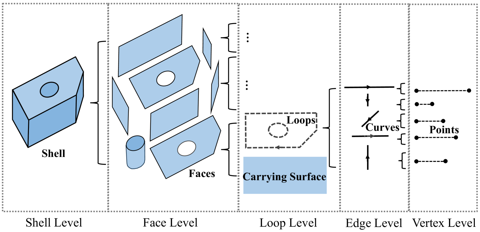
Figure 1: Geometric and topological elements in B-rep models.

A B-rep model encompasses various topological relationships, including hierarchical (e.g., vertex-edge connections), cyclic (e.g., edges forming a loop), and parallel (e.g., adjacent faces within a shell). In this work, different topological embedding methods are provided for these relationships, as detailed below and illustrated in Fig. 2. In the following discussion, we assume that the geometric embeddings of vertices, edges, and faces have already been made available, allowing us to focus exclusively on the topological aspects of B-rep embedding.

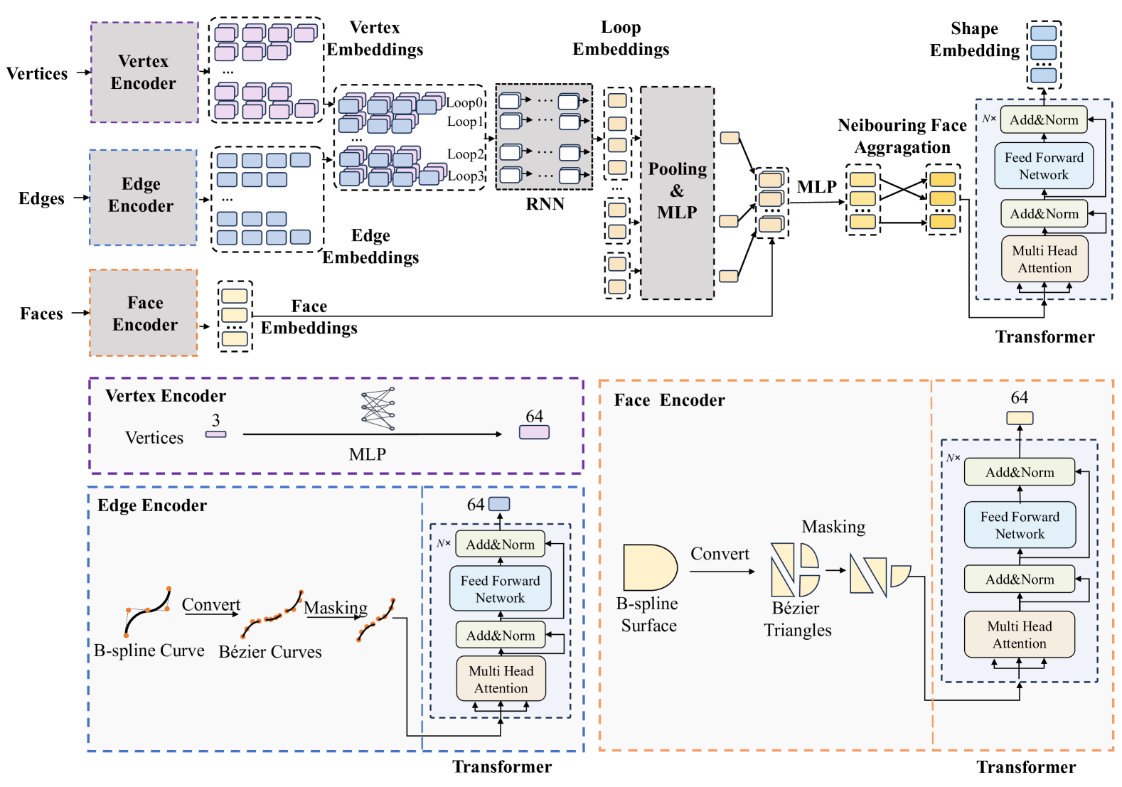
Figure 2: Overall framework of B-rep embedding.

Vertex-Edge Aggregation. The connections between vertices and edges follow a regular pattern: each edge connects to two vertices. Given this structured connectivity, we aggregate information by concatenating the embeddings of the two vertices with the edge embedding. Specifically, for an edge $e_{k}$ connected to vertices $v_{i}$ and $v_{j}$, with embeddings $E(v_{i})$, $E(v_{j})$, and $E(e_{k})$, respectively, the aggregation is done as follows:

$$E(e_{k})\longleftarrow\text{Concat}(E(e_{k}),E(v_{i}),E(v_{j})).$$ (1)

A practical note should be made here. Some might argue that combining vertex embeddings with edge embeddings is unnecessary since the underlying curve segment already encodes endpoint information. However, explicitly incorporating vertex embeddings allows edges sharing the same vertex to exchange information more effectively. Without this, the network would need to learn these connections itself, adding unnecessary complexity to the learning process.

Edge-Loop Aggregation. Unlike the previous aggregation, the number of edges in a loop varies. Also, these edges form a closed circuit, meaning there is no inherent ordering among them, although each edge has an immediate previous and next edge. To address this, we use a recurrent neural network (RNN) to aggregate the edge embeddings. However, loops do not have a distinct start or end, which is typically required to run RNNs. To resolve this, we break the loop at a random edge and unfold it into a linear format that the RNN can process; padding is then added before the start and after the end (Fig. 3). This padding process allows the RNN to focus on the loop’s cyclic connections without being biased by a particular breaking point. The RNN then takes this padded sequence as input.

Mathematically, let the unfolded edge sequence be $\{e_{1},e_{2},\dots,e_{n},e_{1}\}$. The padded version is then:

$$\{e_{n},e_{1},e_{2},\dots,e_{n},e_{1},e_{2}\}.$$ (2)

Applying an RNN to this padded sequence is represented by the following equation:

$$h_{i}=\tanh((W_{he}E(e_{i})+W_{hh}h_{i-1})W_{h})$$ (3)

where $h_{i}$ is the $i$-th hidden state of the RNN, $W_{he}$ and $W_{hh}$ are the weights used to convert the edge embeddings and the previous hidden state into a new hidden state representation, respectively. The matrix $W_{h}$ is used to transform the combined representation into the final hidden state.

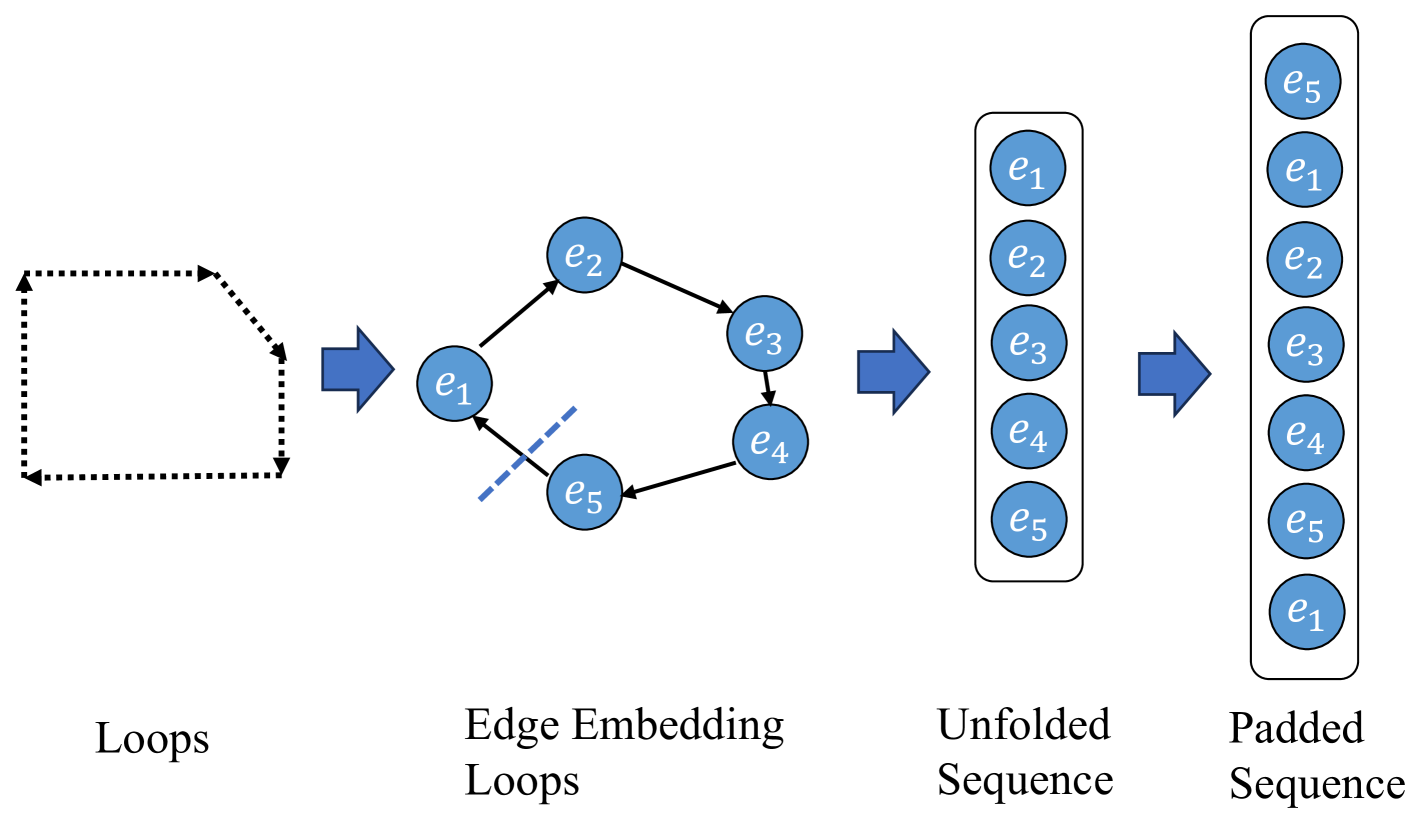
Figure 3: The process of unfolding and padding a loop.

Loop-Face Aggregation. Loops define the boundaries of faces, with each face having one outer boundary loop and a variable number of inner boundary loops (or holes). Since there is no inherent order among the inner boundary loops, we first apply mean and max pooling to their embeddings to generate two aggregated embeddings that capture their overall characteristics. We then use an additional multilayer perceptron (MLP) to combine these two aggregated embeddings with the embedding of the outer boundary loop, producing a unified loop embedding, which is finally concatenated with the face embedding. Specifically, the MLP consists of two layers, featuring a hidden state of size 256 and producing an embedding of size 64.

Let a face be denoted by $f_{i}$, its outer boundary loop be $l_{0}$, and inner boundary loops be $\{l_{1},\dots,l_{n}\}$. The above aggregation process can be mathematically expressed as:

$$E(f_{i})\longleftarrow \text{Concat}(E(f_{i}),$$

$$MLP(Concat(E(l_{0}),$$

$$\text{MeanPooling}(E(l_{1}),\dots,E(l_{n})),$$

$$\text{MaxPooling}(E(l_{1}),\dots,E(l_{n})))))$$ (4)

where $E(\cdot)$ denotes the embedding of a loop or a face.

Face-Shell Aggregation. A shell is formed by a group of connected faces. In most cases, a B-rep solid model simply consists of a single closed shell. However, shells can vary in many ways, such as the number of faces, disjoint components, or internal voids. Since our goal is to achieve a face-based tokenization of B-rep models, we aggregate each face’s embedding with those of its 1-ring neighboring faces. This aggregation captures local contextual information while ensuring overlapping embeddings among faces. Such overlap is particularly beneficial for the attention mechanism in Transformers to effectively model global contextual information across the entire shell.

Specifically, given a face $f_{i}$ and its neighboring faces $\{f_{1},\dots,f_{n}\}$, we apply mean and max pooling to their embeddings to generate two aggregated embeddings that capture their overall characteristics, following a similar approach to loop-face aggregation. We then use a MLP (two layers of sizes 512 and 64) to combine these aggregated embeddings into a unified neighboring face embedding. Finally, we concatenate this with the embedding of the central face $f_{i}$:

$$E(f_{i})\longleftarrow \text{Concat}(E(f_{i}),$$

$$MLP(Concat($$

$$\text{MeanPooling}(E(f_{1}),\dots,E(f_{n})),$$

$$\text{MaxPooling}(E(f_{1}),\dots,E(f_{n})))))$$ (5)

where $E(\cdot)$ denotes the embedding of a face.

The above aggregation methods are applied sequentially, with the output of each step serving as the input for the next. This process ensures that each face embedding preserves its individual geometric and topological properties while incorporating contextual information from its neighboring vertices, edges, loops, and faces. The resulting face embeddings are then used as tokens in Transformers, enabling effective global feature learning across the entire B-rep model.

3.2 Geometric Embedding of B-rep Models

Geometric embedding must handle three types of data: vertices, edges, and faces. A vertex is represented by 3D coordinates, an edge is defined as a curve segment, and a face corresponds to a trimmed surface. To generate meaningful latent embeddings for these elements, we employ the autoencoder (AE) method [52], which encodes input data into a latent space and then reconstructs it back to its original form, as shown in Fig. 4. It is an unsupervised learning method.

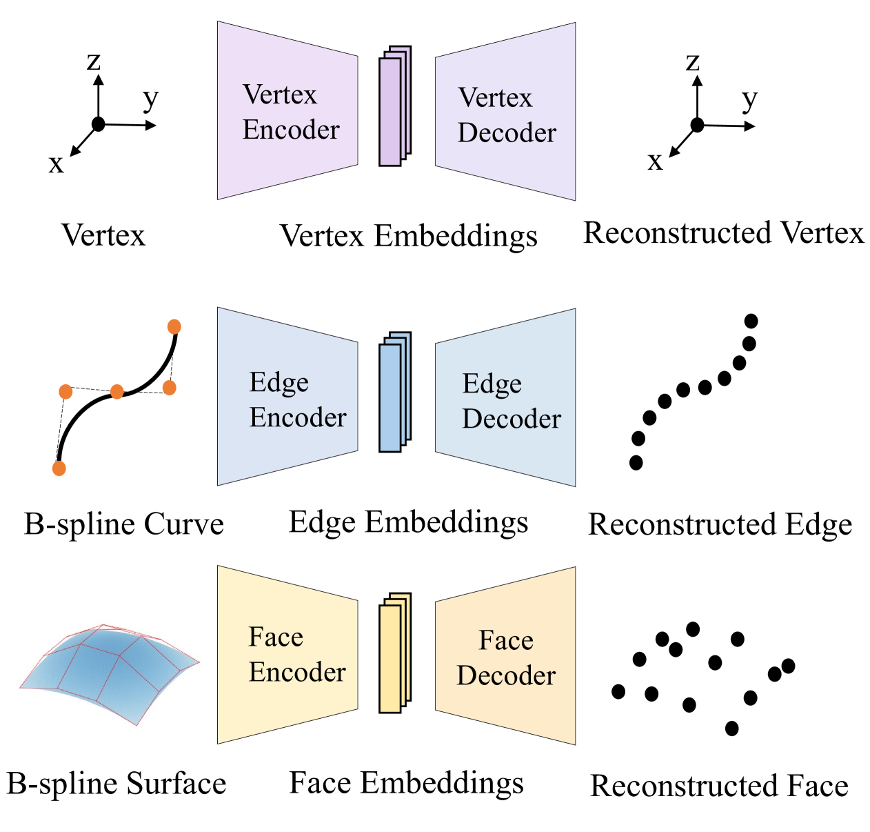
Figure 4: The latent embeddings learnt via autoencoder method.

3.2.1 Vertex Embedding

For vertex embedding, it is straightforward, and we can simply use MLPs. Specifically, we leverage an AE to learn latent embeddings for each vertex.

The encoder, composed of 2 linear layers of size 64, takes the 3D coordinates of the vertex as input and maps it to a latent space of dimension 64. The decoder, consisting of 2 MLP layers outputs an embedding of dimension 3 and reconstructs the vertex with its coordinates.

The reconstructed coordinates are then compared with the original coordinates, and the reconstruction is minimized to ensure effective learning of the underlying geometric feature of the vertex.

Specifically, we just use the distance function as the loss:

$$\mathcal{L}_{\text{recon}}=\|\mathbf{\hat{P}}-\mathbf{P}\|^{2},$$ (6)

where $\mathbf{\hat{P}}$ and $\mathbf{P}$ are the ground truth and reconstructed points, respectively.

3.2.2 Edge Embedding

An edge is represented as a curve segment, which, in its most general form, is defined by a B-spline curve along with its start and end parameters. A B-spline curve $\mathbf{C}(t)$ is defined as:

$$\mathbf{C}(t)=\sum_{i=0}^{n}N_{i,p}(t)\mathbf{P}_{i},$$ (7)

where $t$ is the curve parameter in the range $[0,1]$, $N_{i,p}(t)$ are the B-spline basis functions of degree $p$, and $\mathbf{P}_{i}$ are the control points. The B-spline basis functions $N_{i,p}(t)$ are defined recursively using the Cox-de Boor recursion formula:

$$N_{i,0}(t)=\begin{cases}1,&u_{i}\leq t<u_{i+1},\\ 0,&\text{otherwise}.\end{cases}$$ (8)

$$N_{i,p}(t)=\frac{t-u_{i}}{u_{i+p}-u_{i}}N_{i,p-1}(t)+\frac{u_{i+p+1}-t}{u_{i+p+1}-u_{i+1}}N_{i+1,p-1}(t),$$ (9)

where the knot vector $U=\{u_{0},u_{1},\cdots,u_{n+p+1}\}$ is a non-decreasing sequence of parameter values.

Directly inputting a B-spline curve into the AE model is challenging due to the varying number of control points, knots, and start/end parameters. To address this, existing methods discretize B-spline curves into fixed-size sampled points or polylines. However, this approach suffers: no universal discretization size suits all cases, and application-specific parameter tuning is required. These limitations highlight the need for a more flexible method that operates entirely in the continuous domain, eliminating discretization while ensuring a fixed-dimensional representation.

Decomposing B-spline Curves into Bézier Curves. Inspired by the geometric equivalence between B-spline and Bézier curves, we decompose a B-spline curve into a sequence of connected Bézier curves. A Bézier curve is a special case of a B-spline curve with no knots and a fixed number of control points when the degree is specified. It is a simpler curve formulation that can be effectively processed by neural networks.

A Bézier curve of degree $n$ is defined as:

$$\mathbf{B}(t)=\sum_{i=0}^{n}B_{i,n}(t)\mathbf{P}_{i},\quad t\in[0,1]$$ (10)

where $\mathbf{P}_{i}$ are the control points, and $B_{i,n}(t)=\binom{n}{i}(1-t)^{n-i}t^{i}$ are the Bernstein basis polynomials of degree $n$.

To convert a B-spline curve into Bézier form, we employ the knot insertion technique, a process that increases the number of knots without altering the curve’s shape, as illustrated by Fig. 5. Specifically, Boehm’s algorithm [53] is applied to insert knots at all interior breakpoints. Given a B-spline curve of degree $p$ with control points $\{\mathbf{P}_{i}\}$ and a non-decreasing knot vector $U=\{u_{0},u_{1},\dots,u_{m}\}$, inserting a knot $u\in[u_{i},u_{i+1}]$ introduces a new control point $\mathbf{P}_{i}^{\prime}$ computed as a weighted average of existing control points:

$$\mathbf{P}_{i}^{\prime}=\alpha_{i}\mathbf{P}_{i-1}+(1-\alpha_{i})\mathbf{P}_{i},$$ (11)

where the blending factor $\alpha_{i}$ is given by:

$$\alpha_{i}=\frac{u-u_{i}}{u_{i+p}-u_{i}},\quad u_{i}\leq u\leq u_{i+p}.$$ (12)

By recursively applying this knot insertion until each segment is defined by exactly $n+1$ control points, where $n$ is the degree of the curve, the B-spline curve is transformed into a sequence of Bézier segments, each spanning a single interval of the refined knot vector.

This above process allows us to represent the original B-spline curve entirely in Bézier form, facilitating subsequent processing steps while maintaining its geometric properties. In this work, we consistently use cubic Bézier curves for all cases, i.e., set the hyperparameter $n=3$.

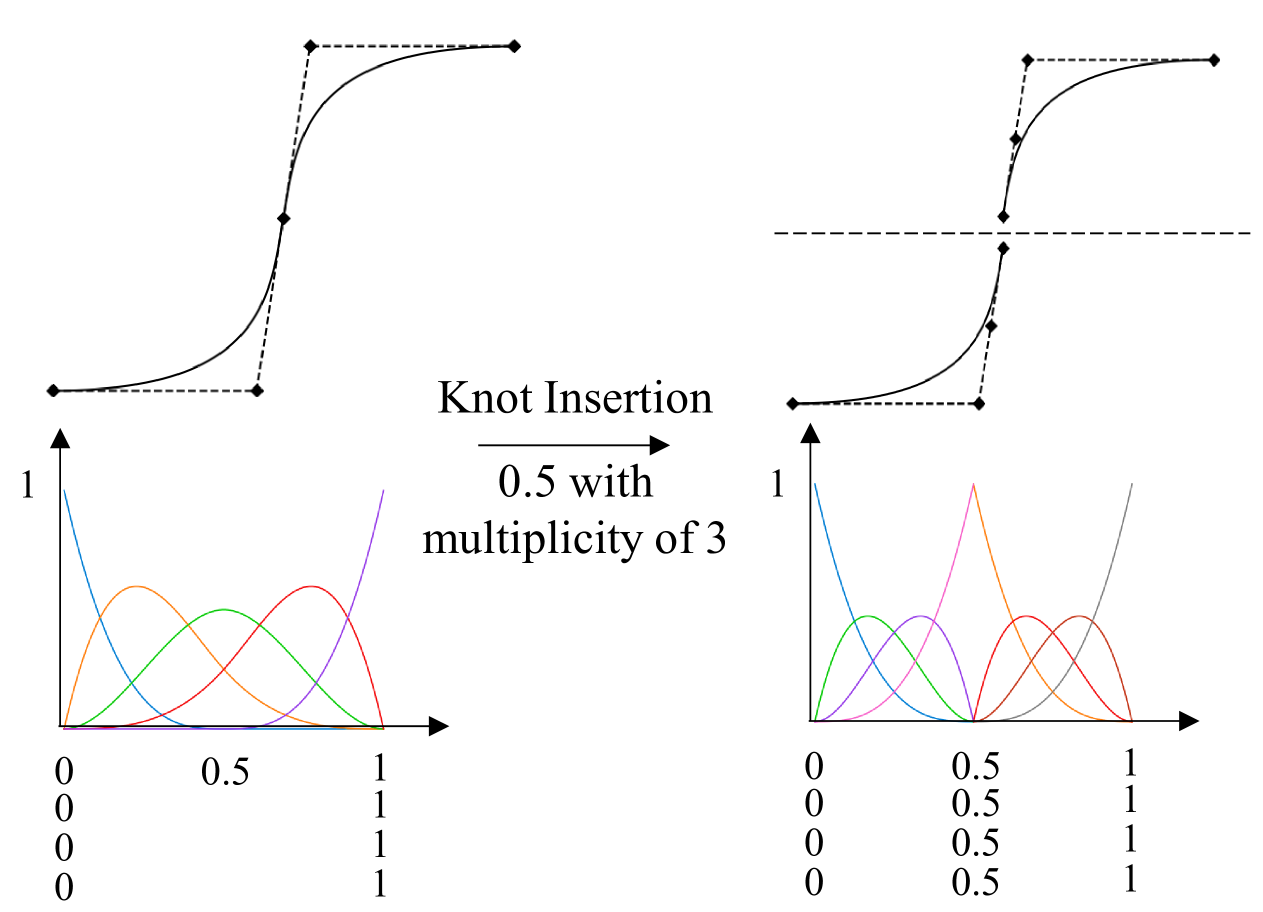
Figure 5: Conversion of a B-spline curve into a sequence of Bézier curves with knot insertion.

Bézier Curve Embedding. After decomposing a B-spline curve into a series of Bézier segments, we employ an AE network to learn compact and meaningful latent embeddings for each segment. The encoder, consisting of three linear layers, takes the four control points of a Bézier curve as input and maps them to a latent space with a dimensionality of 64. Conversely, the decoder, also comprising three linear layers, reconstructs the original Bézier curve by generating a set of 3D points and their corresponding normals from the latent representation and a set of randomly sampled parameters.

The reconstructed points and normals are then compared to those of the original Bézier curve, and the reconstruction error is minimized to ensure effective learning of the underlying geometric structure of the Bézier curves.

Specifically, we utilize a combination of point-wise distance loss and normal consistency loss, defined as:

$$\mathcal{L}_{\text{recon}}=\lambda_{p}\sum_{j}\|\mathbf{\hat{P}}_{j}-\mathbf{P}_{j}\|^{2}+\lambda_{n}\sum_{j}\left(1-\mathbf{\hat{N}}_{j}\cdot\mathbf{N}_{j}\right),$$ (13)

where $\mathbf{P}_{j}$ and $\mathbf{\hat{P}}_{j}$ represent the ground truth and reconstructed points, respectively, and $\mathbf{N}_{j}$ and $\mathbf{\hat{N}}_{j}$ denote the corresponding normals. The hyperparameters $\lambda_{p}$ and $\lambda_{n}$ balance the contributions of point accuracy and normal consistency.

Reassembling Bézier Embeddings into B-spline Embeddings. Given a sequence of Bézier curve embeddings $E(c_{i})$ for $i=0,1,2,\dots,n$, we aggregate these embeddings to obtain an embedding for the original B-spline curve using a Transformer encoder. Specifically, the embedding $E(e)$ is computed as:

$$E(e)=MeanPooling\left(\text{Encoder}\left(E_{pos}(c_{1}),E_{pos}(c_{2}),\dots,E_{pos}(c_{n})\right)\right),$$ (14)

where $E_{\text{pos}}(c_{i})$ denotes the $i$-th curve embedding added with cosine positional embedding. The resulting edge embedding $E(e)$ is extracted from the transformer’s output at the first position, corresponding to $E^{\prime}$. The encoder is a Transformer encoder with 2 layers, 4 attention heads, and a hidden dimension of 512.

3.2.3 Face Embedding

Similar to edge embedding, we decompose each B-spline surface into a collection of connected triangular Bézier patches, known as Bézier triangles. While rectangular Bézier patches (Bézier rectangles) are more commonly used, they struggle to match the shape of trimmed B-spline surfaces near their boundaries. In contrast, Bézier triangles offer greater flexibility while remaining continuous, knot-free, and having a fixed number of control points when the degree is specified, making them well-suited for deep learning.

Our decomposition follows a two-step conversion. First, for regular (untrimmed) B-spline surfaces, we apply knot insertion to transform the surface into a grid of connected Bézier rectangles. Then, leveraging the property that a Bézier rectangle can be split into two Bézier triangles along its diagonal without altering the surface geometry [54], we further convert these Bézier rectangles into Bézier triangles, resulting in a structured representation ideal for deep learning.

For trimmed B-spline surfaces, we extend the above approach by segmenting the trimmed domain and embedding it within the Bézier rectangle representation using knot insertion. If a Bézier rectangle lies entirely within the trimmed parametric domain, the previous rectangle-to-triangle conversion applies directly. If a Bézier rectangle intersects the trimming curves in the parameter domain (p-curves, as illustrated in Fig. 6), we perform the diagonal split as well, but with an additional step to refine the portion inside the trimmed region to ensure it aligns with the actual surface shape. This ensures that the final representation accurately preserves the true geometry of the trimmed surface while maintaining a structured Bézier triangle format. The following content provides a detailed explanation of this process.

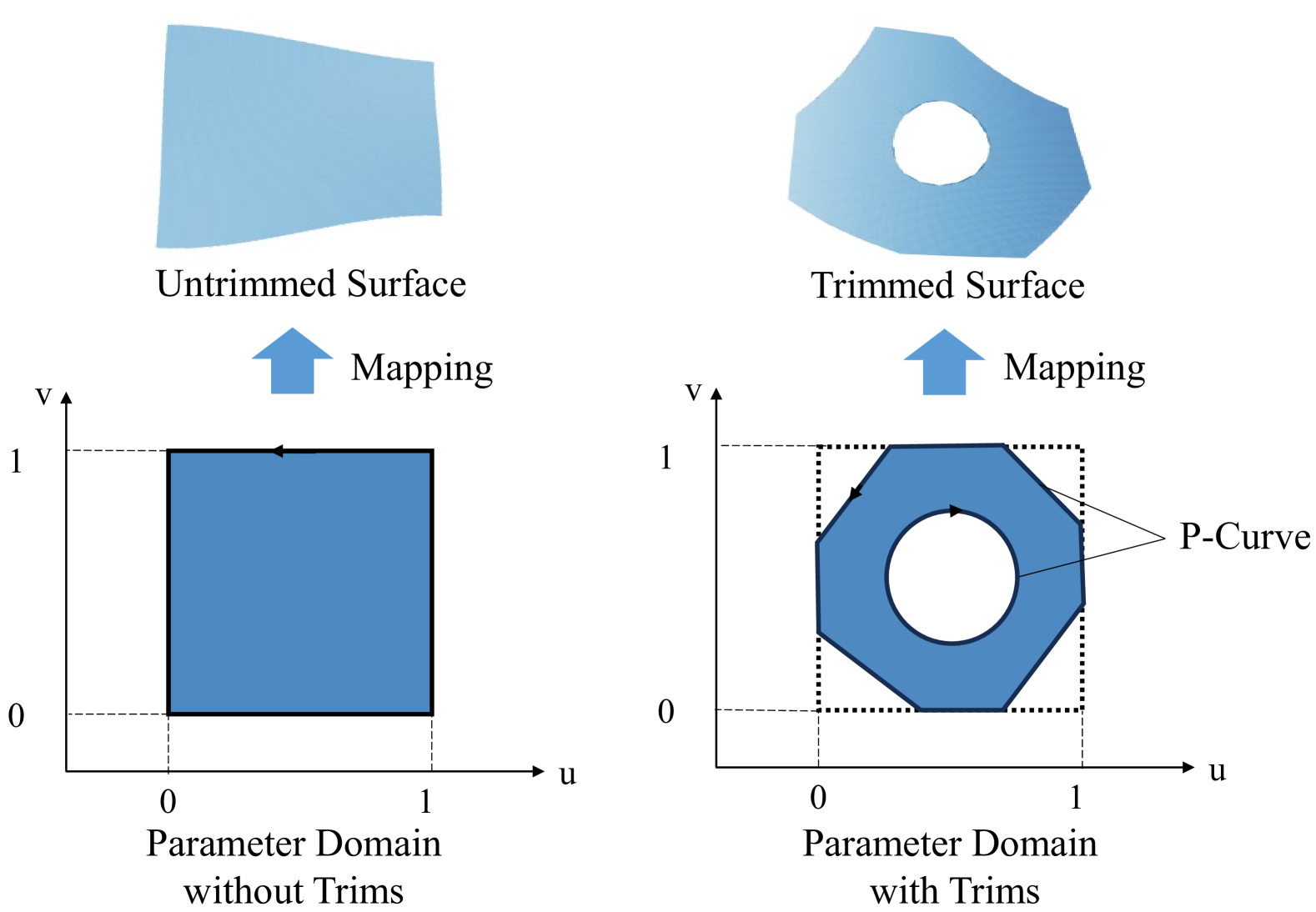
Figure 6: B-spline surfaces: a complete surface and its rectangular parameter domain (left); a trimmed surface and its corresponding parameter domain (right).

Surfaces and Their Trimming. A B-spline surface $\mathbf{S}(u,v)$ is defined as:

$$\mathbf{S}(u,v)=\sum_{i=0}^{n}\sum_{j=0}^{m}N_{i,p}(u)N_{j,q}(v)\mathbf{P}_{i,j},\quad u,v\in[0,1],$$ (15)

where $\mathbf{P}_{i,j}$ are the control points arranged in a 2D grid, and $N_{i,p}(u)$ and $N_{j,q}(v)$ are the B-spline basis functions of degrees $p$ and $q$, respectively. The basis functions follow the Cox-de Boor recursion formula, similar to the curve case.

A trimmed surface consists of an underlying B-spline surface $\mathbf{S}(u,v)$ and a set of p-curves, which are typically loops of B-spline curves defined in the parametric $(u,v)$ domain. These trimming curves outline the valid region of the surface while discarding the exterior portions.

Converting Untrimmed Surfaces to Bézier Triangles. The conversion process extends the 1D decomposition of B-spline curves into Bézier curves to 2D. First, we apply Eq. (11) along the $u$-direction to refine the surface in $u$-parameter space, followed by the same refinement along the $v$-direction. This two-step knot insertion increases the number of control points, forming a structured grid of Bézier rectangles that represent the same shape as the B-spline surface.

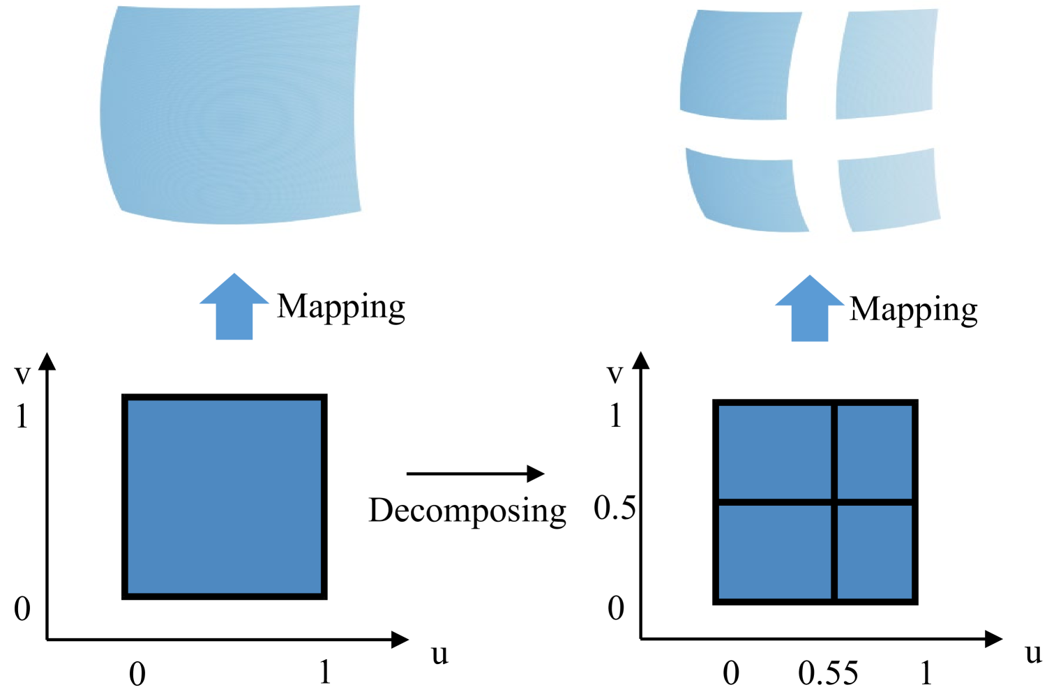
Figure 7: Decomposing a B-spline surface into Bézier rectangles.

Once the B-spline surface is expressed as a grid of Bézier rectangles, each rectangle is split into two Bézier triangles along its diagonal by leveraging the method presented in [54]. The derivations in [54] are complex; thus, we provide a simplified version here.

A Bézier rectangle of degree $(m,n)$ in the parametric domain $(u,v)$ is given by the tensor-product form:

$$\mathbf{S}(u,v)=\sum_{i=0}^{m}\sum_{j=0}^{n}B_{i}^{m}(u)B_{j}^{n}(v)\mathbf{P}_{i,j},\quad 0\leq u,v\leq 1,$$ (16)

where $B_{i}^{m}(u)$ and $B_{j}^{n}(v)$ are Bernstein basis polynomials.

To split the rectangle along the diagonal from $(0,1)$ to $(1,0)$ (Fig. 8), we introduce two sets of barycentric coordinates:

$$s =u, t =v, s+t \leq 1,$$ (17)

$$s^{\prime} =1-u, t^{\prime} =1-v, s^{\prime}+t^{\prime} \leq 1.$$ (18)

Rewriting the univariate Bernstein polynomials in terms of these new barycentric coordinates:

$$B_{i}^{m}(u)=\sum_{h=0}^{m-i}B_{i,h}^{m}(s,t),\quad B_{j}^{n}(v)=\sum_{k=0}^{n-j}B_{k,j}^{n}(s,t),$$ (19)

where the bivariate Bernstein basis is:

$$B_{i,h}^{m}(s,t)=\binom{m}{i,h}s^{i}t^{h}(1-s-t)^{m-i-h},\quad\binom{m}{i,h}=\frac{m!}{i!h!(m-i-h)!}.$$ (20)

Thus, their product expands as:

$$B_{i}^{m}(u)B_{j}^{n}(v)=\sum_{h=0}^{m-i}\sum_{k=0}^{n-j}B_{i,h}^{m}(s,t)B_{k,j}^{n}(s,t).$$ (21)

Using the identity:

$$B_{i,h}^{m}(s,t)B_{k,j}^{n}(s,t)=\frac{\binom{m}{i,h}\binom{n}{k,j}\binom{m+n}{i+k,h+j}}{\binom{m+n}{i+k,h+j}}B_{i+k,h+j}^{m+n}(s,t),$$ (22)

we obtain:

$$B_{i}^{m}(u)B_{j}^{n}(v)=\sum_{h=0}^{m-i}\sum_{k=0}^{n-j}\frac{\binom{i+k}{i}\binom{h+j}{j}\binom{m+n-k-i-h-j}{m-i-h}}{\binom{m+n}{n}}B_{i+k,h+j}^{m+n}(s,t).$$ (23)

This means we can rewrite the Bézier rectangle $S(u,v)$ as:

$$\mathbf{S}(u,v)=\sum_{i=0}^{m}\sum_{j=0}^{n}\sum_{h=0}^{m-i}\sum_{k=0}^{n-j}\frac{\binom{i+k}{i}\binom{h+j}{j}\binom{m+n-k-i-h-j}{m-i-h}}{\binom{m+n}{n}}\mathbf{P}_{i,j}B_{i+k,h+j}^{m+n}(s,t).$$ (24)

By defining new control points:

$$\mathbf{V}_{a,b}=\frac{\sum_{i=0}^{a}\sum_{j=\max\{0,\,b-m+i\}}^{\min\{b,\,n-a+i\}}\binom{a}{i}\binom{b}{j}\binom{m+n-a-b}{m-a-i}}{\binom{m+n}{n}}\mathbf{P}_{i,j},$$ (25)

we can rewrite $\mathbf{S}(u,v)$ in terms of barycentric coordinates:

$$\mathbf{S}(u,v)=\sum_{a,b\geq 0}^{a+b\leq m+n}B_{a,b}^{m+n}(s,t)\mathbf{V}_{a,b}.$$ (26)

Thus, the resulting Bézier triangle (the bottom-left one) is:

$$\mathbf{T}_{1}(s,t)=\sum_{i,j\geq 0}^{i+j\leq m+n}B_{i,j}^{m+n}(s,t)\mathbf{V}_{i,j},\quad 0\leq s,t,s+t\leq 1.$$ (27)

Similarly, the second Bézier triangle (the top-right one) is derived by applying the same transformation symmetrically.

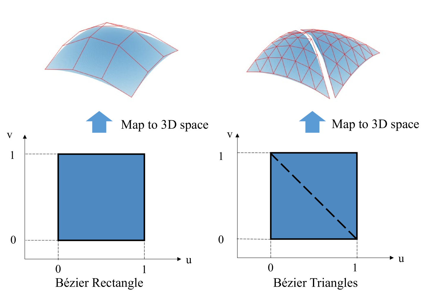
Figure 8: Convert Bézier rectangles into two Bézier triangles.

Converting Trimmed Surfaces to Bézier Triangles. The conversion here follows a similar workflow to that of untrimmed surfaces, with an additional step to handle Bézier rectangles intersecting p-curves, as shown in Fig. 9a. Directly applying a diagonal split to such incomplete Bézier rectangles does not guarantee alignment with the actual surface shape along the surface boundary. To address this, we first subdivide the Bézier rectangle until the p-curve passes through a pair of its diagonal points (Fig. 9b). This ensures a precise classification of the intersection region, allowing for a clean diagonal split.

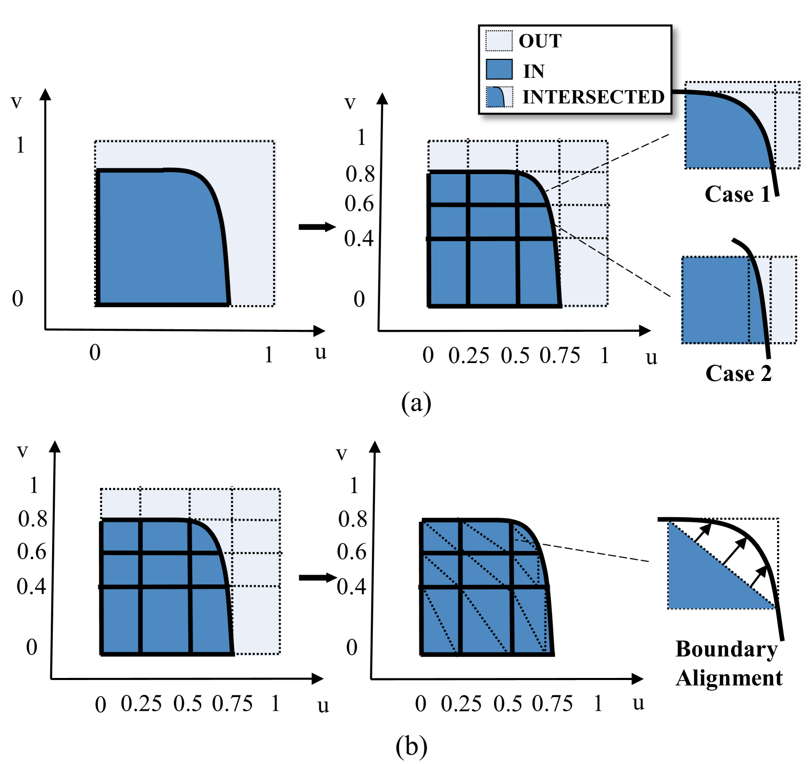
Figure 9: Conversion of a trimmed B-spline surface into triangular Bézier patches: (a) Convert B-spline surface to Bézier rectangles; (b) Convert Bézier rectangles To Bézier triangles.

Once subdivided, we apply the standard diagonal split and identify the Bézier triangle within the trimming domain. To ensure geometric alignment with the original surface along the trimming boundary, we refine its control points using the following least-squares optimization:

$$\min_{\mathbf{V}_{i,j}}\sum_{k=0}^{N}\left\|\mathbf{P}_{k}-\sum_{i,j\geq 0}^{i+j\leq m+n}B_{i,j}^{m+n}(u_{k},v_{k})\mathbf{V}_{i,j}\right\|^{2}+\lambda\sum_{i,j\geq 0}^{i+j\leq m+n}\left\|\mathbf{V}_{i,j}-\mathbf{V}_{i,j}^{\text{orig}}\right\|^{2}$$ (28)

where $\mathbf{P}_{k}$ are sampled surface points along the trimming boundary, $\mathbf{V}_{i,j}^{\text{orig}}$ are the control points obtained from the initial rectangle-to-triangle conversion, and $\lambda$ is a weighting parameter controlling the balance between surface fitting and shape preservation. The first term ensures the Bézier triangle closely aligns with the surface along the trimming boundary, while the second term prevents excessive deviation from its original shape. This optimization problem is a standard least-squares problem, which reduces to solving a linear system. Finally, the resulting Bézier triangles not only ensure smooth transitions with existing triangles but also maintain a well-structured Bézier triangle framework.

Bézier Triangle Embedding. Each Bézier triangle can be represented by its control points. For a Bézier triangle of degree $2p$, the number of control points is $(2p+1)(2p+2)/2$, with each control point consisting of 3D-coordinates and weight, forming a tensor of $(2p+1)(p+1)\times 4$. We then facilitate an AE network to learn a Bézier triangle embedding. The encoder, composed of three layers, takes the control points as input and maps them to a latent space of dimension 64. The decoder, consisting of 2 MLP layers, reconstructs the original Bézier triangle by generating a set of 3D points and their corresponding normals from the latent representation and a set of randomly sampled parameters. These reconstructed points and normals are then compared with those of the original Bézier triangle, and the reconstruction error is minimized to ensure effective learning of the underlying geometric structure of the Bézier triangle.

Specifically, we use a combination of point-wise distance loss and normal consistency loss:

$$\mathcal{L}_{\text{recon}}=\lambda_{p}\sum_{j}\|\mathbf{\hat{P}}_{j}-\mathbf{P}_{j}\|^{2}+\lambda_{n}\sum_{j}\left(1-\mathbf{\hat{N}}_{j}\cdot\mathbf{N}_{j}\right),$$ (29)

where $\mathbf{P}_{j}$ and $\mathbf{\hat{P}}_{j}$ are the ground truth and reconstructed points, respectively, and $\mathbf{N}_{j}$ and $\mathbf{\hat{N}}_{j}$ are the corresponding normals. The hyperparameters $\lambda_{p}$ and $\lambda_{n}$ balance the contribution of point accuracy and normal consistency.

Reassemble Triangular Bézier Embeddings into B-spline Surface Embeddings. Given a sequence of triangular Bézier embeddings $E(t_{i})$ for $i=0,1,2,\dots,n$, we aggregate these embeddings to obtain an embedding for the original B-spline surface using a Transformer encoder. Specifically, the embedding $E(f)$ is computed as:

$$E(f)=MeanPooling\left(\text{Encoder}\left(E_{pos}(t_{1}),E_{pos}(t_{2}),\dots,E_{pos}(t_{n})\right)\right),$$ (30)

where $E_{\text{pos}}(t_{i})$ denotes the $i$-th triangular Bézier embedding added with cosine positional embedding. The resulting face embedding $E(f)$ is extracted from the transformer’s output at the first position, corresponding to $E^{\prime}$. The encoder is a Transformer encoder with 2 layers, 8 attention heads, and a hidden dimension of 512.

3.3 Training BRT

By integrating the preceding geometric and topological embedding modules, we obtain a B-rep tokenization network, which, when paired with a Transformer encoder, forms the BRT network. We first train BRT using the AE architecture to learn initial, rough embeddings of B-rep models, then fine-tune these embeddings on domain-specific tasks like part classification and feature recognition. A masking technique is also introduced during training to enhance BRT’s robustness and generalizability.

Rough Training via AE. Given a B-rep model, BRT encodes it into latent embeddings. To ensure these embeddings are compact and geometrically meaningful, we use the AE architecture and require it to reconstruct the original B-rep shape from the embeddings. This is achieved by appending a decoder to BRT. The decoder is intentionally kept simple, consisting of only three MLP layers. This forces the embeddings to capture sufficient geometric information for effective reconstruction of the B-rep model.

Specifically, after tokenizing the B-rep model, we obtain a set of face embeddings, which are passed into a Transformer encoder with 2 attention layers, 8 heads, and an embedding dimension of 64. Unlike traditional Transformer encoders, our model does not include a positional encoding module, as the face embeddings have the advantage of order-independence. The output latent embeddings from the Transformer encoder are then passed to the three-layer decoder. This decoder takes the latent embeddings, along with additional point positions, as input and outputs predictions about whether the input points lie inside, outside, or on the B-rep model.

If the decoder consistently makes correct predictions, it indicates that the shape of the B-rep model has been effectively captured by the latent embeddings. To encourage such predictions during training, we use the following cross-entropy loss:

$$\mathcal{L}_{\text{recon}}=-\frac{1}{N}\sum_{i=1}^{N}\sum_{c=1}^{3}y_{i,c}\log(\hat{y}_{i,c})$$ (31)

where $N$ is the number of input points, and $y_{i,c}$ and $\hat{y}_{i,c}$ respectively represent the ground truth and predicted probabilities for class $c={In,Out,On}$ of the $i$-th input point.

Fine Training by Domain-Specific Tasks. The rough training described above is unsupervised, producing general latent embeddings that can be further refined for specific tasks. To enhance task-specific performance, we fine-tune BRT through supervised learning on key B-rep modeling tasks like part classification and feature recognition, which have applications in CAD model searching and CAD/CAM integration [19, 22]. Labeled data for this fine-tuning comes from a proprietary dataset MechCAD collected by our team, as well as publicly available datasets—FebWave [55], SolidLetters [19], MFCAD++ [1], and Fusion 360 Gallery [47].

Training by Masking. To enhance the robustness and generalizability of BRT, we apply a masking technique [56] that randomly drops a subset (e.g., 25% or even 50%) of Bézier triangle embeddings during training and then forces BRT to continue to generate correct outputs despite the missing data. This encourages BRT to learn the structural and contextual relationships within B-rep models, rather than memorizing exact input values, which can lead to overfitting.

4 Results

In this section, a range of experiments are performed to evaluate BRT on classification and segmentation tasks on various datasets. The BRT is trained using PyTorch and runs on an NVIDIA GeForce RTX 4090 D GPU. A learning rate is utilized with an initial learning rate of 0.0001, as well as the ADAM optimizer [57]. The size of each batch is 16, and we perform the BRT training in 350 epochs. With BRT as the solid model encoder, the classification, machining feature recognition and modeling operations recognition experiments are performed, which are shown in Sec. 4.1, Sec. 4.3 and Sec. 4.4, respectively.

4.1 Classification

This section presents comprehensive experimental results on several open-source classification datasets, including FebWave [55], SolidLetters [19], and MechCAD, to evaluate the performance of the proposed BRT. For all datasets, we employ a random split of 70% for training, 15% for validation, and 15% for testing.

4.2 3D Shape Classification

We first assess our method on the task of 3D shape classification. For comparison, we train UV-Net [19] using 10x10 grids, and AAGNet [22] with all attributes enabled. Since AAGNet is originally designed for segmentation tasks, we adapt it for classification by utilizing the global features produced by its graph encoder as the solid’s global features and adding a classification head composed of two MLP layers to generate the classification logits. We exclude BRepNet [47] from the comparison because its network architecture is not tailored for classification tasks.

All models are trained for up to 350 epochs using cross-entropy loss and the Adam optimizer with $\beta_{1}=0.001$ and $\beta_{2}=0.999$. As shown in Table 1, our method achieves the highest classification accuracy across all datasets. This highlights the effectiveness of our continuous geometric and hierarchical topological embeddings, enabling our approach to outperform existing methods.

Fig. 10 illustrates some classification results on the test set of the MechCAD dataset compared with two other methods. Specifically, Model 1 is excessively complex, and AAGNet fails to convert certain solid models into graphs successfully.

Table 1: Classification performance comparison across datasets.

Dataset	Network	Input Geometry	Accuracy (%)
MechCAD	BRT (Ours)	Bézier patches	82.01
	UV-Net	Grids	81.31
	AAGNet	Grids+ Attributes	74.72
FebWave	BRT (Ours)	Bézier patches	98.83
	UV-Net	Grids	93.49
	AAGNet	Grids+ Attributes	96.33
SolidLetters	BRT (Ours)	Bézier patches	97.28
	UV-Net	Grids	95.82
	AAGNet	Grids + Attributes	96.99

4.3 Machining Feature Recognition

In the machining feature recognition tasks, we compared BRT with UV-Net [19], AAGNet [22], and BRepNet [47] using the MFCAD++ dataset [1]. We train UV-Net and AAGNet using network configurations similar to those employed in the classification experiments, and we train BRepNet with the winged edge kernel.

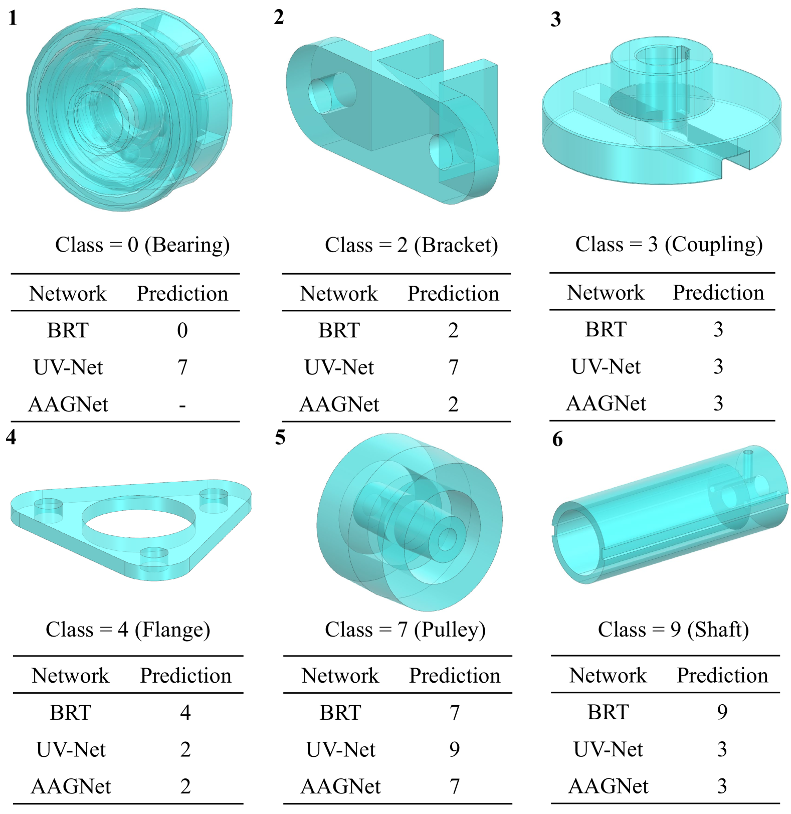
Figure 10: Examples of classification on MechCAD compared to UV-Net.

Table 2 presents the feature recognition accuracy and mean Intersection over Union (IoU) for each network on MFCAD++. Our method outperforms both UV-Net and BRepNet, as demonstrated by some of our feature recognition results in Fig. 11. However, AAGNet achieves higher accuracy and IoU than our approach. This discrepancy arises because AAGNet effectively handles planar faces, which constitute the majority of faces in the MFCAD++ dataset. In contrast, our continuous geometry representation does not leverage its advantages on planar faces as effectively within this dataset, unlike in datasets with more complex geometries such as MechCAD and SolidLetters.

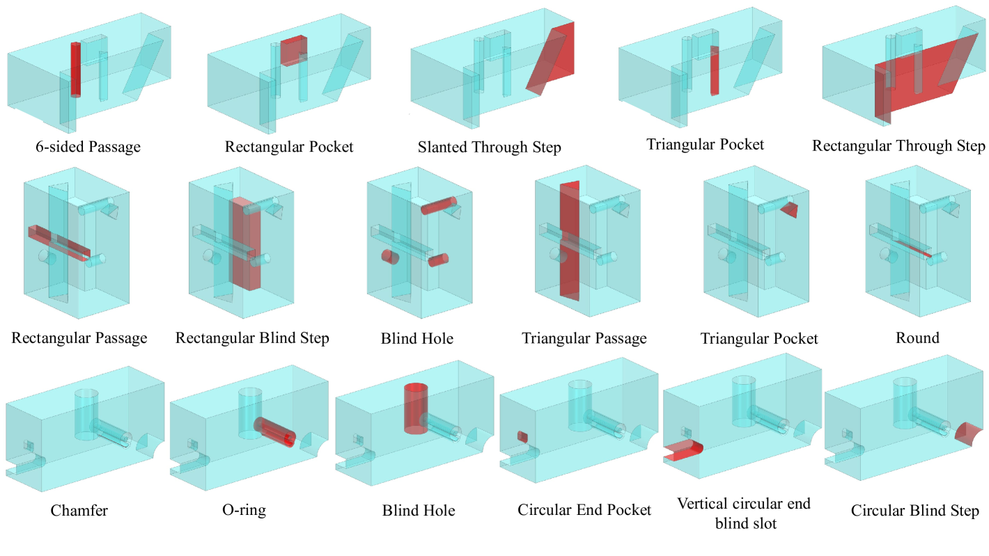
Figure 11: Examples of feature recognition on MFCAD++.

Table 2: Feature recognition performance comparison on MFCAD++.

Network	Accuracy (%)	IoU (%)
BRT (Ours)	99.26	97.94
UV-Net	99.02	96.85
AAGNet	99.29	98.64
BRepNet	99.22	97.75

4.4 Segmentation on CAD Modeling Operations

This section presents extensive experimental results on the Fusion 360 Gallery Dataset [47] to further evaluate the performance of BRT on the segmentation task involving more complex solids.

Table 2 shows the face accuracy and mean Intersection over Union (IoU) for each network on the Fusion 360 Gallery dataset. Our method outperforms all other approaches in terms of face accuracy. Notably, the Fusion 360 Gallery dataset, derived from real-world data, exhibits higher structural and geometric complexity compared to MFCAD++. Consequently, the accuracy and IoU of all methods are lower on this dataset compared to MFCAD++.

Table 3: Segmentation on modeling operations performance comparison on Fusion 360 Gallery.

Network	Accuracy (%)	IoU (%)
BRT (Ours)	90.47	70.16
UV-Net	89.03	66.47
AAGNet	75.53	82.45
BRepNet	90.19	68.92

4.5 Ablation Study

In this subsection, we examine the impact of various input features and network components on the machining feature recognition task using the MFCAD++ dataset. The study is structured as follows:

1. BRT (Original): The BRT network, incorporating all input features and modules.

2. w.o. Masking: We removed the masking strategy described in Sec. 3.3.

3. w.o. Trim: A variant of BRT that disregards the trimming curves of each B-rep face and transforms the untrimmed surfaces into Bézier triangles, as outlined in Sec. 3.2.3.

4. GCN: We replaced the original topological encoder with a Graph Convolutional Network (GCN) module.

The ablation study results are presented in Table 4. Our findings indicate that the masking strategy significantly enhances the performance of the BRT model. Additionally, the model utilizing trimmed surfaces performs slightly better than its non-trimmed counterpart. Moreover, compared to the GCN, which serves as a general-purpose module for graph-based data, our specialized topological encoder demonstrates superior performance on the B-rep MFCAD++ dataset. These experiments confirm the effectiveness of our proposed methods.

Table 4: Ablation study with input features and components of BRT on the MFCAD++ for feature recognition task.

Model	Accuracy (%)
BRT (Original)	99.26
w.o. Masking	94.78
w.o. Trim	98.99
GCN	99.26

5 Conclusion

In this paper, we introduced BRT, a novel transformer-based encoder specifically designed for learning B-rep (Boundary Representation) data. Our approach involves converting faces into triangular Bézier patches and edges into Bézier curves, thereby preserving the continuous geometry inherent in B-rep models. Additionally, we developed a topological embedding strategy to effectively represent the irregular structure of B-rep data. To thoroughly capture the relationships between geometric and topological elements, we fully leveraged the attention mechanism within our transformer architecture. This comprehensive approach demonstrated state-of-the-art performance in both classification and segmentation tasks across several B-rep datasets. Furthermore, we introduced a new B-rep dataset, MechCAD, which more accurately reflects real-world model data, underscoring the practical applicability of our work.

Limitations & Future Work. Our work presents certain limitations that offer opportunities for future improvement. During the conversion of trimmed B-spline surfaces into triangular Bézier patches, ensuring that the Bézier triangles on the boundaries precisely conform to the boundary curves can be challenging. Often, these boundary curves cannot be exactly represented as B-spline curves, leading to approximation errors. Although the approximation accuracy of these boundary Bézier triangles is high, the residual errors may still affect the performance of tasks such as classification and machining feature recognition.

Moreover, while transformers have demonstrated exceptional performance with large datasets, the current availability of B-rep data remains limited. We anticipate that the emergence of larger and more diverse datasets will unlock significant potential for our BRT method. Also, the transformer decoder could be utilized to autoregressively generate B-rep models, further enhancing the capabilities and applications of our approach.

Appendix A MechCAD Dataset

We collect B-rep models from the Internet and construct a dataset containing 10,897 CAD models stored in STEP file format, which is split into 10 classes, including Bearing, Bolt, Bracket, Coupling, Flange, Gear, Nut, Pulley, Screw, Shaft. Fig. 12 shows some examples from MechCAD datasets. Fig. 13 shows the distribution of the different solid clases within the MechCAD dataset. There is an average of 1,090 models per class in the dataset.

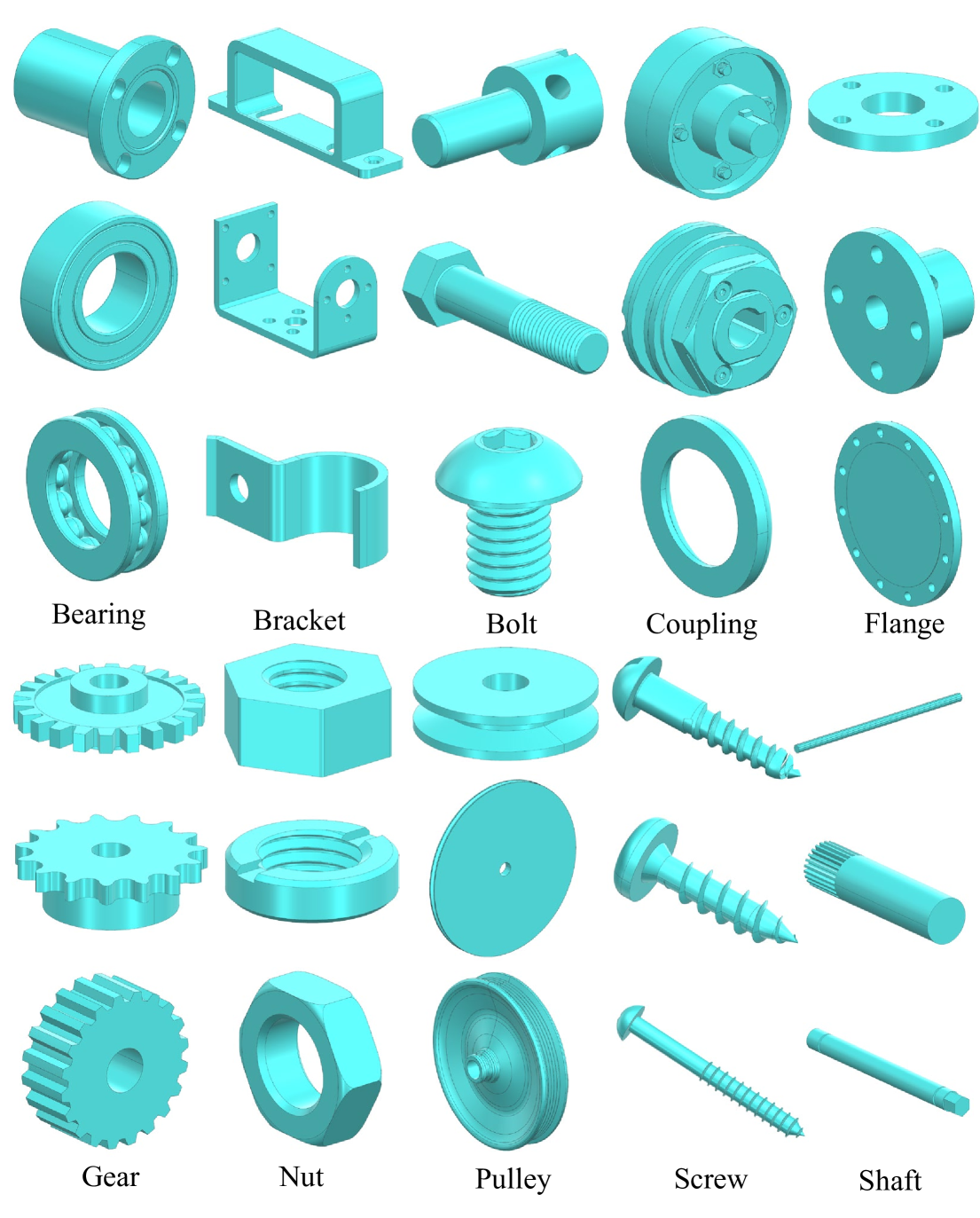
Figure 12: Some examples from MechCAD.

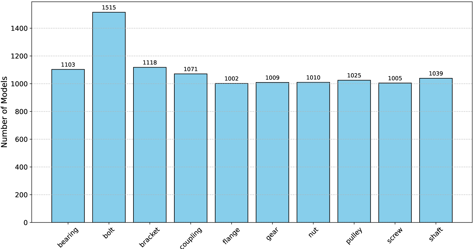
Figure 13: Per-class distribution of solids in the MechCAD dataset.

Appendix B Other Datasets

FebWave Dataset [55]. The FebWave dataset is a small, labeled, and imbalanced collection of 5,373 3D shapes categorized into 52 mechanical part classes, such as brackets, gears, and o-rings.

SolidLetters Dataset [19]. The SolidLetters dataset comprises 96k 3D shapes generated by randomly extruding and filleting the 26 alphabet letters. These shapes are organized into 2,002 style categories based on different fonts.

MFCAD++ Dataset [1]. This dataset contains 59,655 CAD models with 24 types of machining features, including both planar and non-planar faces. Each CAD model includes between 3 to 10 machining features, enhancing the dataset’s difficulty and diversity.

Fusion 360 Gallery Dataset [47]. The Fusion 360 Gallery dataset is a curated collection of 35,858 3D models and designs sourced from Autodesk’s Fusion 360 Gallery. The segmentation dataset is provided in STEP file format, with labels assigning one of eight categories to each face: ExtrudeSide, ExtrudeEnd, CutSide, CutEnd, Fillet, Chamfer, RevolveSide, and RevolveEnd.

Appendix C Implementation Details of Other Methods

We implemented each of the methods across different datasets. The implementation details of each network can be found below:

• UV-Net implementation: github.com/AutodeskAILab/UV-Net/tree/main/uvnet.

• BrepNet implementation: github.com/AutodeskAILab/BRepNet.

• AAGNet implementation: github.com/whjdark/AAGNet.

References

- [1] A. R. Colligan, T. T. Robinson, D. C. Nolan, Y. Hua, W. Cao, Hierarchical CADNet: Learning from B-reps for machining feature recognition, Computer-Aided Design 147 (2022) 103226.
- [2] Q. Zou, Y. Wu, Z. Liu, W. Xu, S. Gao, Intelligent CAD 2.0, Visual Informatics (2024).
- [3] Y. Zhao, Q. Zou, G. Luo, J. Wu, S. Chen, D. Gao, M. Xuan, F. Wang, Tpms2step: error-controlled and c2 continuity-preserving translation of tpms models to step files based on constrained-pia, Computer-Aided Design 173 (2024) 103726.
- [4] X. Chen, S. Gao, Y. Yang, S. Zhang, Multi-level assembly model for top-down design of mechanical products, Computer-Aided Design 44 (10) (2012) 1033–1048.
- [5] Q. Zou, Y. Gao, G. Luo, S. Chen, Meta-meshing and triangulating lattice structures at a large scale, Computer-Aided Design 174 (2024) 103732.
- [6] M. Li, C. Lin, W. Chen, Y. Liu, S. Gao, Q. Zou, Xvoxel-based parametric design optimization of feature models, Computer-Aided Design 160 (2023) 103528.
- [7] Q. Zou, J. Zhao, Iso-parametric tool-path planning for point clouds, Computer-Aided Design 45 (11) (2013) 1459–1468.
- [8] C. R. Qi, L. Yi, H. Su, L. J. Guibas, PointNet++: Deep hierarchical feature learning on point sets in a metric space, Advances in neural information processing systems 30 (2017).
- [9] H. Zhang, S. Zhang, Y. Zhang, J. Liang, Z. Wang, Machining feature recognition based on a novel multi-task deep learning network, Robotics and Computer-Integrated Manufacturing 77 (2022) 102369.
- [10] Z. Zhang, P. Jaiswal, R. Rai, FeatureNet: Machining feature recognition based on 3D convolution neural network, Computer-Aided Design 101 (2018) 12–22.
- [11] D. Peddireddy, X. Fu, A. Shankar, H. Wang, B. G. Joung, V. Aggarwal, J. W. Sutherland, M. B.-G. Jun, Identifying manufacturability and machining processes using deep 3D convolutional networks, Journal of Manufacturing Processes 64 (2021) 1336–1348.
- [12] H. Su, S. Maji, E. Kalogerakis, E. Learned-Miller, Multi-view convolutional neural networks for 3D shape recognition, in: Proceedings of the IEEE international conference on computer vision, 2015, pp. 945–953.
- [13] P. Shi, Q. Qi, Y. Qin, P. J. Scott, X. Jiang, A novel learning-based feature recognition method using multiple sectional view representation, Journal of Intelligent Manufacturing 31 (2020) 1291–1309.
- [14] Q. Zou, H.-Y. Feng, A robust direct modeling method for quadric b-rep models based on geometry–topology inconsistency tracking, Engineering with Computers 38 (4) (2022) 3815–3830.
- [15] Q. Zou, H.-Y. Feng, A decision-support method for information inconsistency resolution in direct modeling of cad models, Advanced Engineering Informatics 44 (2020) 101087.
- [16] Q. Zou, H.-Y. Feng, S. Gao, Variational direct modeling: A framework towards integration of parametric modeling and direct modeling in CAD, Computer-Aided Design 157 (2023) 103465.
- [17] Q. Zou, J. Zhang, B. Deng, J. Zhao, Iso-level tool path planning for free-form surfaces, Computer-Aided Design 53 (2014) 117–125.
- [18] J. Ding, Q. Zou, S. Qu, P. Bartolo, X. Song, C. C. Wang, Stl-free design and manufacturing paradigm for high-precision powder bed fusion, CIRP Annals 70 (1) (2021) 167–170.
- [19] P. K. Jayaraman, A. Sanghi, J. G. Lambourne, K. D. Willis, T. Davies, H. Shayani, N. Morris, UV-Net: Learning from boundary representations, in: Proceedings of the IEEE/CVF Conference on Computer Vision and Pattern Recognition, 2021, pp. 11703–11712.
- [20] J. Lee, C. Yeo, S.-U. Cheon, J. H. Park, D. Mun, BRepGAT: Graph neural network to segment machining feature faces in a B-rep model, Journal of Computational Design and Engineering 10 (6) (2023) 2384–2400.
- [21] S. Zhang, Z. Guan, H. Jiang, X. Wang, P. Tan, BrepMFR: Enhancing machining feature recognition in B-rep models through deep learning and domain adaptation, Computer Aided Geometric Design 111 (2024) 102318.
- [22] H. Wu, R. Lei, Y. Peng, L. Gao, AAGNet: A graph neural network towards multi-task machining feature recognition, Robotics and Computer-Integrated Manufacturing 86 (2024) 102661.
- [23] A. Vaswani, N. Shazeer, N. Parmar, J. Uszkoreit, L. Jones, A. N. Gomez, L. Kaiser, I. Polosukhin, Attention is all you need, Advances in Neural Information Processing Systems 30 (2017) 5998–6008.
- [24] A. Dosovitskiy, An image is worth 16x16 words: Transformers for image recognition at scale, arXiv preprint arXiv:2010.11929 (2020).
- [25] M.-H. Guo, J. Cai, Z.-N. Liu, T. Mu, R. R. Martin, S.-M. Hu, PCT: Point cloud transformer, in: Computational Visual Media, Springer, 2021, pp. 22–35.
- [26] T. Brown, B. Mann, N. Ryder, M. Subbiah, J. D. Kaplan, P. Dhariwal, A. Neelakantan, P. Shyam, G. Sastry, A. Askell, et al., Language models are few-shot learners, Advances in neural information processing systems 33 (2020) 1877–1901.
- [27] L. Li, Y. Zheng, M. Yang, J. Leng, Z. Cheng, Y. Xie, P. Jiang, Y. Ma, A survey of feature modeling methods: Historical evolution and new development, Robotics and Computer-Integrated Manufacturing 61 (2020) 101851.
- [28] Q. Zou, H.-Y. Feng, Push-pull direct modeling of solid CAD models, Advances in Engineering Software 127 (2019) 59–69.
- [29] Q. Zou, L. Zhu, J. Wu, Z. Yang, Splinegen: Approximating unorganized points through generative AI, Computer-Aided Design 178 (2025) 103809.
- [30] G. Farin, Triangular Bernstein-Bézier patches, Computer Aided Geometric Design 3 (2) (1986) 83–127.
- [31] W. Cao, Z. Yan, Z. He, Z. He, A comprehensive survey on geometric deep learning, IEEE Access 8 (2020) 35929–35949.
- [32] C. R. Qi, H. Su, K. Mo, L. J. Guibas, PointNet: Deep learning on point sets for 3D classification and segmentation, in: Proceedings of the IEEE conference on computer vision and pattern recognition, 2017, pp. 652–660.
- [33] Y. Wang, Y. Sun, Z. Liu, S. E. Sarma, M. M. Bronstein, J. M. Solomon, Dynamic graph CNN for learning on point clouds, ACM Transactions on Graphics (tog) 38 (5) (2019) 1–12.
- [34] R. Hanocka, A. Hertz, N. Fish, R. Giryes, S. Fleishman, D. Cohen-Or, Meshcnn: a network with an edge, ACM Transactions on Graphics (ToG) 38 (4) (2019) 1–12.
- [35] Y. Feng, Y. Feng, H. You, X. Zhao, Y. Gao, MeshNet: Mesh neural network for 3D shape representation, in: Proceedings of the AAAI conference on artificial intelligence, Vol. 33, 2019, pp. 8279–8286.
- [36] A. Lahav, A. Tal, Meshwalker: Deep mesh understanding by random walks, ACM Transactions on Graphics (TOG) 39 (6) (2020) 1–13.
- [37] P.-S. Wang, Y. Liu, Y.-X. Guo, C.-Y. Sun, X. Tong, O-CNN: Octree-based convolutional neural networks for 3D shape analysis, ACM Transactions On Graphics (TOG) 36 (4) (2017) 1–11.
- [38] H. Zhao, L. Jiang, C.-W. Fu, J. Jia, K. Vladlen, Point transformer, in: Proceedings of the IEEE/CVF International Conference on Computer Vision, 2021, pp. 16259–16268.
- [39] X. Yu, L. Tang, Y. Rao, T. Huang, J. Zhou, J. Lu, Point-BERT: Pre-training 3D point cloud transformers with masked point modeling, in: Proceedings of the IEEE/CVF Conference on Computer Vision and Pattern Recognition, 2022, pp. 19313–19322.
- [40] Y. Li, X. He, Y. Jiang, H. Liu, Y. Tao, L. Hai, Meshformer: High-resolution mesh segmentation with graph transformer, in: Computer Graphics Forum, Vol. 41, Wiley Online Library, 2022, pp. 37–49.
- [41] S.-M. Hu, Z.-N. Liu, M.-H. Guo, J.-X. Cai, J. Huang, T.-J. Mu, R. R. Martin, Subdivision-based mesh convolution networks, ACM Transactions on Graphics (TOG) 41 (3) (2022) 1–16.
- [42] J. Mao, Z. Wang, Z. Li, B. Jia, H. Zhu, S. Li, X. Zhang, J. Sun, Voxel transformer for 3D object detection, arXiv preprint arXiv:2109.02497 (2021).
- [43] J.-L. Jia, S.-W. Zhang, Y.-R. Cao, X.-L. Qi, WeZhu, Machining feature recognition method based on improved mesh neural network, Iranian Journal of Science and Technology, Transactions of Mechanical Engineering 47 (4) (2023) 2045–2058.
- [44] B. Shi, S. Bai, Z. Zhou, X. Bai, DeepPano: Deep panoramic representation for 3-D shape recognition, IEEE Signal Processing Letters 22 (12) (2015) 2339–2343.
- [45] W. Liu, D. Anguelov, D. Erhan, C. Szegedy, S. Reed, C.-Y. Fu, A. C. Berg, SSD: Single shot multibox detector, in: Computer Vision – ECCV 2016, Springer, 2016, pp. 21–37.
- [46] W. Cao, T. Robinson, Y. Hua, F. Boussuge, A. R. Colligan, W. Pan, Graph representation of 3d CAD models for machining feature recognition with deep learning, in: International design engineering technical conferences and computers and information in engineering conference, Vol. 84003, American Society of Mechanical Engineers, 2020, p. V11AT11A003.
- [47] J. G. Lambourne, K. D. Willis, P. K. Jayaraman, A. Sanghi, P. Meltzer, H. Shayani, Brepnet: A topological message passing system for solid models, in: Proceedings of the IEEE/CVF Conference on Computer Vision and Pattern Recognition, 2021, pp. 12773–12782.
- [48] X. Ma, C. Qin, H. You, R. Ranftl, Y. Liu, Rethinking transformers in point clouds: A simple residual attention network, Advances in Neural Information Processing Systems 35 (2022) 4470–4483.
- [49] K. Lin, L. Wang, Z. Liu, Y. Zhu, End-to-end human pose and mesh reconstruction with transformers, in: Proceedings of the IEEE/CVF Conference on Computer Vision and Pattern Recognition, 2021, pp. 1954–1963.
- [50] P.-S. Wang, Octformer: Octree-based transformers for 3D point clouds, ACM Transactions on Graphics (TOG) 42 (4) (2023) 1–11.
- [51] A. G. Requicha, Representations for rigid solids: Theory, methods, and systems, ACM Computing Surveys (CSUR) 12 (4) (1980) 437–464.
- [52] G. E. Hinton, R. R. Salakhutdinov, Reducing the dimensionality of data with neural networks, Science 313 (5786) (2006) 504–507.
- [53] L. Piegl, W. Tiller, The NURBS book, Springer Science & Business Media, 2012.
- [54] R. N. Goldman, D. J. Filip, Conversion from bézier rectangles to bézier triangles, Computer-Aided Design 19 (1) (1987) 25–27.
- [55] A. Angrish, B. Craver, B. Starly, “FabSearch”: A 3D CAD model-based search engine for sourcing manufacturing services, Journal of Computing and Information Science in Engineering 19 (4) (2019) 041006.
- [56] K. He, X. Chen, S. Xie, Y. Li, P. Dollár, R. Girshick, Masked autoencoders are scalable vision learners, in: Proceedings of the IEEE/CVF Conference on Computer Vision and Pattern Recognition, 2022, pp. 16000–16009.
- [57] D. P. Kingma, Adam: A method for stochastic optimization, arXiv preprint arXiv:1412.6980 (2014).