Near-Inertial Pollard Waves Modeling the Arctic Halocline

Abstract.

We present an explicit exact solution to the governing equations describing the vertical structure of the Arctic Ocean region centered around the North Pole. The solution describes a stratified water column with three constant-density regions: a motionless bottom layer, a top layer with uniform velocity and a middle layer - the halocline - described by nonhydrostatic, near-inertial Pollard waves.

1. Introduction

The Arctic Ocean, located in the Northern Hemisphere and encompassing the North Pole, is a small ocean about $4000\,\mathrm{km}$ long and $2500\,\mathrm{km}$ wide, covering an area of around 10 million $\,\mathrm{km}^{2}$. It includes two main deep basins (around $4000\,\mathrm{m}$ deep) separated by the underwater Lomonosov Ridge, the Amerasian Basin (divided into the Makarov and Canada basins), and the smaller Eurasian Basin (divided into the Amundsen and Nansen basins), and is surrounded by shallow seas (less than $400\,\mathrm{m}$ deep): the Barents Sea, the Kara Sea, the Laptev Sea, the Siberian Sea, the Chukchi Sea and the Beaufort Sea (see [2] or [37]).
The primary oceanic inflows are from the Atlantic Ocean through the Fram Strait and the Barents Sea, and from the Pacific Ocean via the Bering Strait. Significant freshwater inflows also come from rivers in North America and Siberia. These inflows are major factors influencing the salinity and temperature variability of the water column, with salinity playing a key role in stratification, creating a halocline rather than a thermocline (which instead is typical of mid-latitudes and equatorial regions). As a matter of fact, one of the main feature of the Arctic Ocean is that it’s predominantly stratified by salinity (hence it is defined as a $\beta$-ocean) rather than by temperature (the so called $\alpha$-oceans) (see[2] or [3]).
Moreover, the central region of Arctic Ocean - the one centered around the North Pole and subject of our analysis - is entirely covered by a relatively thin (not exceeding $2\,\mathrm{m}$ of thickness) layer of sea ice, which reduces in summer when temperature increases. Due to the global warming, the sea ice is rapidly declining, and the Arctic region is warming faster than the global average, due to the process known as Arctic amplification. This makes the Arctic highly vulnerable to climate change, potentially leading to an ice-free Arctic Ocean in summer and with thinner and more mobile sea ice in winter. The transition to a seasonally ice-free Arctic will profoundly affect Arctic oceanography, the marine ecosystems it supports, and the global climate (see [38]).
In addition to the atmospheric conditions, the Arctic sea ice is influenced by the sea water beneath it. The Arctic Ocean is stratified into a cold and fresh surface mixed layer (SML), with a depth between $5$ to $100$ meters, a halocline below the mixed layer with a base depth ranging from $40$ to $200$ meters, and a layer of warmer and saltier Atlantic Water (AW) (see [24]). The depths of the boundaries of this layers varies mainly according to temperature and presence of ice. In general, it can be said that in winter, with lower temperatures and increased ice presence, their depth increases, whereas in summer, these decrease (see [29]).
The halocline is a region of strong stratification, which prevents interaction of the ice cover with AW heat by the direct surface-generated mixing of the SML (see [32] and [18] for an in-detail description of the Arctic water column and its main physical processes). Consequently, the halocline layer, situated above the saltier and denser water, is fundamental for the formation of the ice cover (see [32]).
The presence of the permanent ice layer makes physical measurements particularly difficult. Hence, due to the lack of data from observation, the theoretical analysis of this region is particularly useful.
The physical processes in the mixed layer, mainly the ice-motion induced by wind and the Transpolar Drift Current (TDC) - the Arctic Ocean current transporting surface waters and sea ice from the Laptev Sea and the East Siberian Sea towards Fram Strait, with a speed of around $0.07\,\mathrm{ms^{-1}}$ around the North Pole - induces a current with magnitude approximately $0.1\,\mathrm{ms^{-1}}$ on the lower boundary of the mixed layer (see [18] and data therein).
The aim of this paper is to describe the halocline layer via an explicit and exact solution of the (approximated) nonlinear equations governing the ocean dynamics. Such a solution will represent nonlinear waves propagating in the direction of the Transpolar Drift Current. Just above the halocline we consider a uniform current, and the layer of Atlantic Water under the halocline is considered in hydrostatic state.
The solution in this study is constructed by adapting the Pollard’s solution, presented in 1970 [31] for surface waves accounting for the effects of Earth’s rotation and extending the remarkable solution provided by Gerstner in [16]. We refer to [5] and [19]. Recently, Gerstner-like solution were used to describe equatorially-trapped waves [6], [7], [8] and to study their linear stability [13], or to study wave-current interactions [12], [25], [26].
Even if within the halocline one could distinguish between the cold halocline layer in the Eurasian Basin, the Pacific Halocline Waters in the Amerasian Basin and the lower halocline water (see [24]), the simplified model we will consider features constant densities in the layers under consideration. The case of depth-dependent densities could be considered in future works, even if density variations are very small within each stratum (see [32]), so accounting for for density variation would not provide substantial differences. Our model features three constant densities, $\rho_{0}$, $\rho_{1}$ and $\rho_{2}$, with $\rho_{0}<\rho_{1}<\rho_{2}$, where $\rho_{0}$ represents the fresh and cold water of the surface mixed layer above the halocline, $\rho_{1}$ is the density of the halocline’s water and $\rho_{2}$ is the density of the saltier and warmer water (AW) below the halocline. See Figure 1.1.

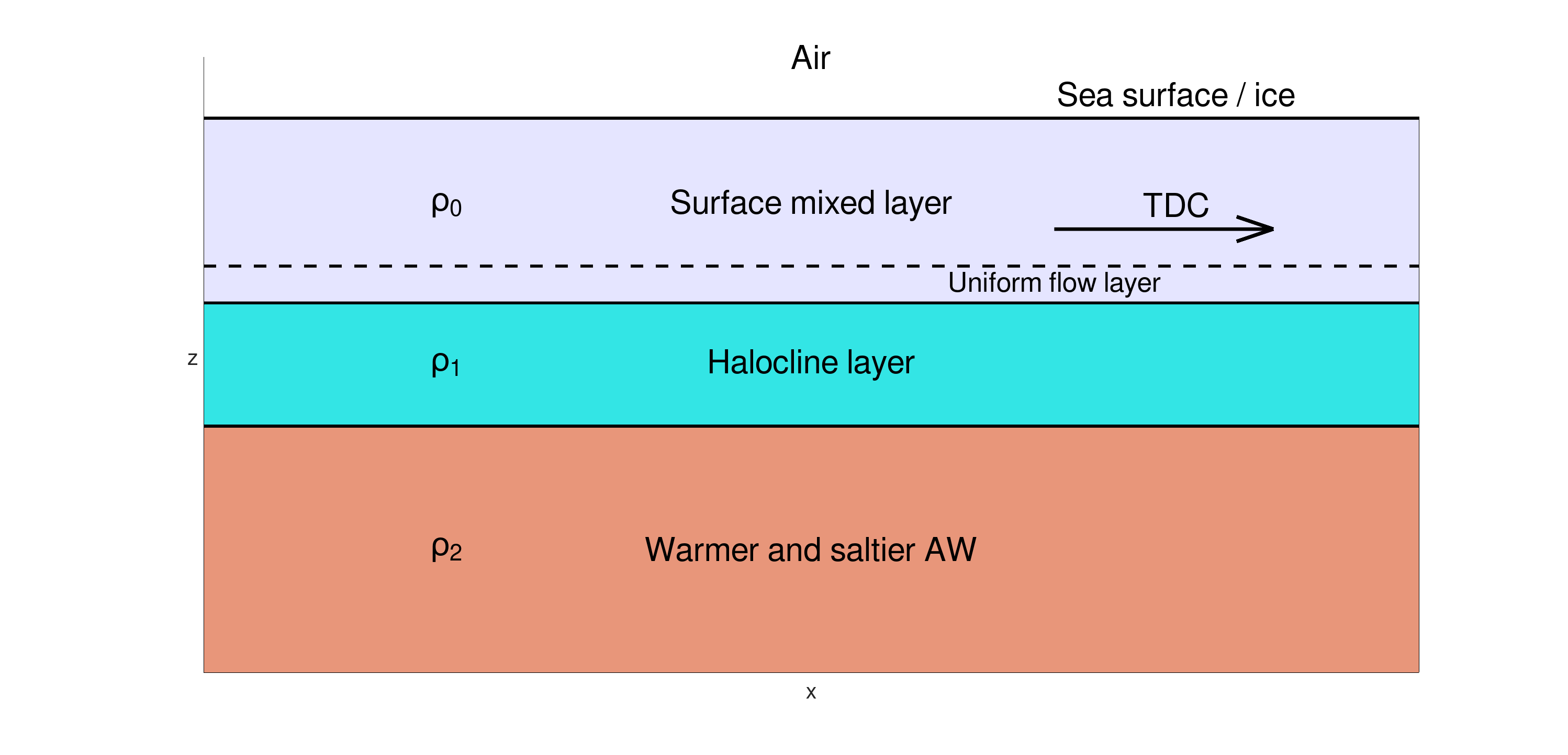
Figure 1.1. A depiction of the model we are considering

More precisely, we assume the following water characteristics (we refer to [34]):

• Surface Mixed Layer: water density $\rho_{0}$, $\mathfrak{T}=-1.5^{\circ}\,\mathrm{C}$, $\mathfrak{S}=34.0\,\mathrm{psu}$;

• Halocline: water density $\rho_{1}$, $\mathfrak{T}=0^{\circ}\,\mathrm{C}$, $\mathfrak{S}=34.2\,\mathrm{psu}$;

• Atlantic Water: water density $\rho_{2}$, $\mathfrak{T}=2^{\circ}\,\mathrm{C}$, $\mathfrak{S}=34.9\,\mathrm{psu}$;

and density variations can be modeled by (see [2] or [37])

$$\frac{d\rho}{\rho}=-\alpha\,d\mathfrak{T}+\beta\,d\mathfrak{S},$$ (1.1)

where $\mathfrak{T}$ is the potential temperature, $\mathfrak{S}$ is the salinity, $\alpha\approx 53\cdot 10^{-6}\,\mathrm{K^{-1}}$ is the thermal expansion coefficient and $\beta\approx 785\cdot 10^{-6}\,\mathrm{kg}\,\mathrm{g^{-1}}$ is the haline contraction coefficient. Both $\alpha$ and $\beta$ depend of the water properties, therefore the value reported here refer only for the Arctic Ocean (see [37]).
We recall that the flow will be considered motionless under the halocline and uniform just above it.

The paper is structured as follow:

• in Section 2 we derive the governing equations. More precisely, as we are investigating the fluid dynamics around the North Pole, where the classical spherical coordinates fail, we need to adopt the rotated spherical coordinates developed in [10], and therefore adapt the tangent-plane, traditional and $f$-plane approximations to this new coordinate system, starting from the Euler equations. Then, by a $2D$ rotation we will align one of the axes with the Transpolar Drift Current in order to simplify the study of the internal waves propagating in its direction;

• Section 3 is devoted to the main result of our analysis. We find an explicit solution, using the Lagrangian description of the flow, detailing the internal wave motion in the halocline by near-inertial Pollard waves propagating parallel to the Transpolar Drift Current. The dispersion relation for the nonlinear waves is obtained imposing the dynamic boundary condition (namely the continuity of the pressure across the two layers: the top and the bottom of the halocline).
  In previous works [12], [21], [26], with only one dynamic boundary condition, two modes of the wave motion were found, one fast mode standard to the theory of internal waves, and a second one, slow, with the period close to the inertial period of the Earth $T_{i}=\frac{2\pi}{f}$. Constantin & Monismith [12] refer to this slow-mode wave as inertial Gerstner wave.
  In this work, imposing two dynamic conditions, one per boundary of the halocline, only the slow mode is show to be relevant. Henceforth, the waves will be near-inertial;

• Section 4 is aimed at the review of some properties of the flow: vorticity, Lagrangian and Eulerian mean velocities, Stokes drift and mass flux;

• in Section 5 we study the linearized version of the problem, still adopting the Lagrangian approach. The near-inertial slow mode is obtained again, and it is shown that the expression for the pressure in the linearized case is an approximation of the one in the nonlinear analysis;

• finally, we conclude in Section 6 with a discussion on the results.

2. Governing (approximated) equations

We consider the Earth to be a sphere of radius $R\approx 6371\,\mathrm{km}$. The classical spherical coordinate system is not suitable for the study of flows in regions centered around the North (and South) Pole, as longitude in undefined at the poles. This result is a consequence of the ‘hairy ball theorem’ (see [4] and [11]). In this section, we review the construction of the rotated spherical coordinate system developed in [10] (see [11] for a detailed exposition) to avoid this problem and we derive the $f$-plane approximation for the Euler equations in this new coordinate system.
Let us start by considering the standard Cartesian coordinate system $(X,Y,Z)$ with basis $(\mathbf{e}_{1},\mathbf{e}_{2},\mathbf{e}_{3})$ positioned at the center $O$ of the Earth, and pointing in the direction $\vec{OZ}$ of the Null Island, $\vec{OE}$ East, $\vec{ON}$ North, respectively, and define the classical spherical coordinates $(\varphi,\theta,r)$, with $\varphi\in[0,2\pi)$ and $\theta\in[-\frac{\pi}{2},\frac{\pi}{2}]$ being the angles of longitude and latitude respectively, and $r$ the distance from Earth’s center. With respect to these coordinates, a point $P$ has position vector

$$\vec{OP}:=\mathbf{r}=r\cos\theta\cos\varphi\mathbf{e}_{1}+r\cos\theta\sin\varphi\mathbf{e}_{2}+r\sin\theta\mathbf{e}_{3}.$$ (2.1)

Namely, the change of coordinates is given by

$$\left\{\begin{array}[]{ll}X=r\cos\theta\cos\varphi,\\ Y=r\cos\theta\sin\varphi,\\ Z=r\sin\theta,\end{array}\right.\qquad\left\{\begin{array}[]{ll}\varphi=\tan^{-1}\left(\frac{Y}{X}\right),\\ \theta=\sin^{-1}\left(\frac{Z}{\sqrt{X^{2}+Y^{2}+Z^{2}}}\right),\\ r=\sqrt{X^{2}+Y^{2}+Z^{2}}.\end{array}\right.$$ (2.2)

Now, let us define a new Cartesian coordinate system $(\mathbf{e}_{1}^{{\dagger}},\mathbf{e}_{2}^{{\dagger}},\mathbf{e}_{3}^{{\dagger}})$ by permuting cyclically the first three Cartesian axes

$$\mathbf{e}_{1}^{{\dagger}}=\mathbf{e}_{3},\quad\mathbf{e}_{2}^{{\dagger}}=\mathbf{e}_{1},\quad\mathbf{e}_{3}^{{\dagger}}=\mathbf{e}_{2}.$$ (2.3)

The associated Cartesian coordinates to $(\mathbf{e}_{1}^{{\dagger}},\mathbf{e}_{2}^{{\dagger}},\mathbf{e}_{3}^{{\dagger}})$ are $(X^{{\dagger}},Y^{{\dagger}},Z^{{\dagger}})$, and, in terms of the associated azimuthal $\theta^{{\dagger}}\in[-\frac{\pi}{2},\frac{\pi}{2}]$ and meridional $\varphi^{{\dagger}}\in[0,2\pi)$ angles (given by the analogous of (2.2)), the coordinates of a point $P$ on the Earth are

$$\vec{OP}:=\mathbf{r}=r\cos\theta^{{\dagger}}\cos\varphi^{{\dagger}}\mathbf{e}_{1}^{{\dagger}}+r\cos\theta^{{\dagger}}\sin\varphi^{{\dagger}}\mathbf{e}_{2}^{{\dagger}}+r\sin\theta^{{\dagger}}\mathbf{e}_{3}^{{\dagger}},$$ (2.4)

Therefore, using (2.3) and equaling (2.1) and (2.4), it follows that

$$\left\{\begin{aligned} &\cos\theta^{{\dagger}}\cos\varphi^{{\dagger}}=\cos\theta\sin\varphi,\\ &\cos\theta^{{\dagger}}\sin\varphi^{{\dagger}}=\sin\theta,\\ &\sin\theta^{{\dagger}}=\cos\theta\cos\varphi.\end{aligned}\right.$$ (2.5)

In this new coordinate system the North Pole has coordinates $\varphi^{{\dagger}}=\frac{\pi}{2},\ \theta^{{\dagger}}=0$, and the solution of the system (2.5) for the Arctic Ocean is

$$\left\{\begin{aligned} &\varphi^{{\dagger}}=\cot^{-1}(\sin\varphi\cot\theta)\in(0,\pi),\\ &\theta^{{\dagger}}=\sin^{-1}(\cos\varphi\cos\theta)\in\left(-\frac{\pi}{2},\frac{\pi}{2}\right).\end{aligned}\right.$$ (2.6)

The unit basis vectors in the rotated spherical coordinates $(\varphi^{{\dagger}},\theta^{{\dagger}},r)$ are $(\mathbf{e}_{\varphi}^{{\dagger}},\mathbf{e}_{\theta}^{{\dagger}},\mathbf{e}_{r})$, given by

$$\left\{\begin{array}[]{ll}\mathbf{e}_{\varphi}^{{\dagger}}=-\sin\varphi^{{\dagger}}\mathbf{e}_{1}^{{\dagger}}+\cos\varphi^{{\dagger}}\mathbf{e}_{2}^{{\dagger}},\\ \mathbf{e}_{\theta}^{{\dagger}}=-\cos\varphi^{{\dagger}}\sin\theta^{{\dagger}}\mathbf{e}_{1}^{{\dagger}}-\sin\varphi^{{\dagger}}\sin\theta^{{\dagger}}\mathbf{e}_{2}^{{\dagger}}+\cos\theta^{{\dagger}}ec^{{\dagger}},\\ \mathbf{e}_{r}^{{\dagger}}=\cos\varphi^{{\dagger}}\cos\theta^{{\dagger}}\mathbf{e}_{1}^{{\dagger}}+\sin\varphi^{{\dagger}}\cos\theta^{{\dagger}}\mathbf{e}_{2}^{{\dagger}}+\sin\theta^{{\dagger}}\mathbf{e}_{3}^{{\dagger}},\end{array}\right.$$ (2.7)

and the corresponding velocity components are $\boldsymbol{u}=(u^{{\dagger}},v^{{\dagger}},w^{{\dagger}})$.
The two coordinate systems are depicted in Figure 2.1.

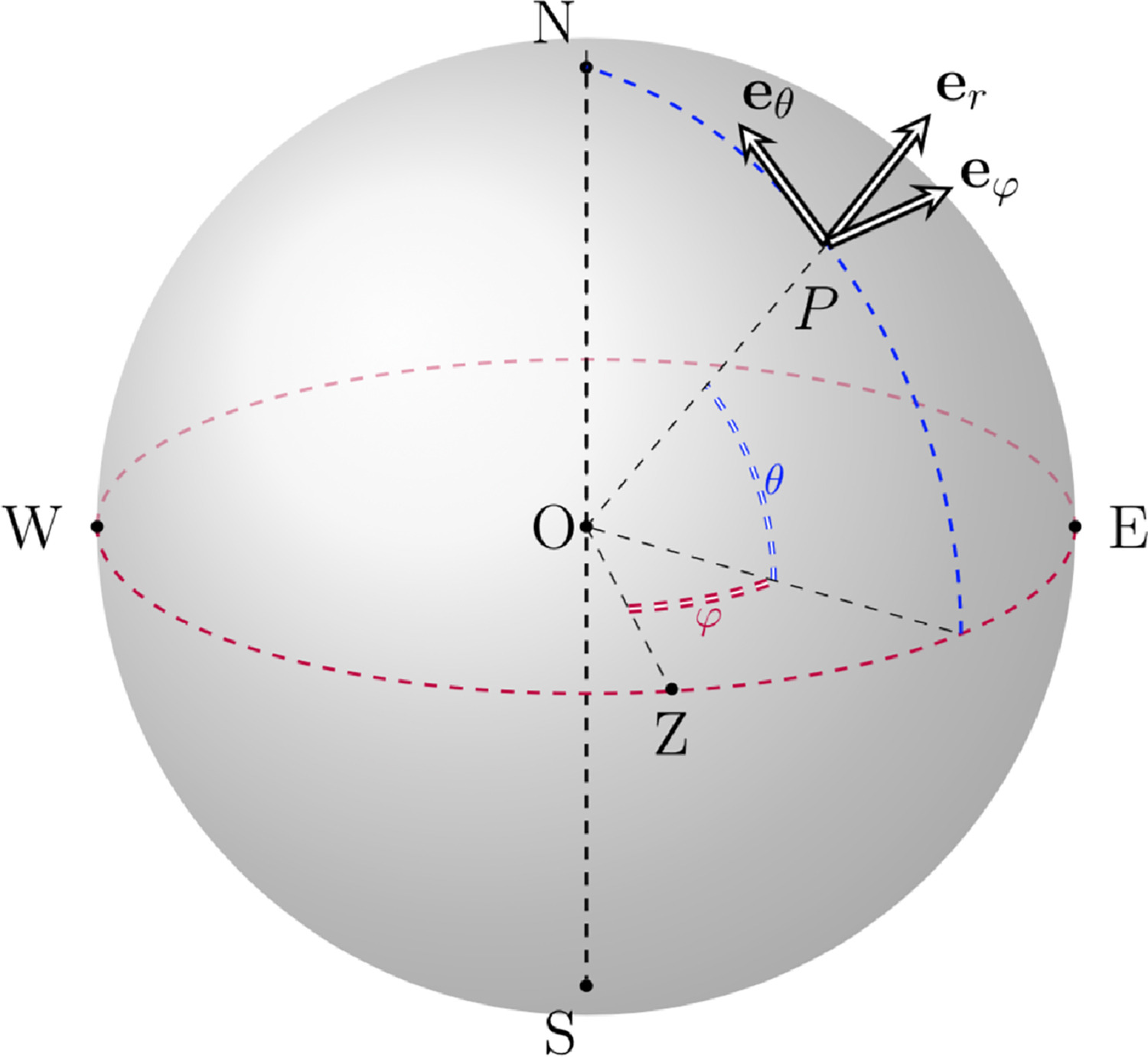
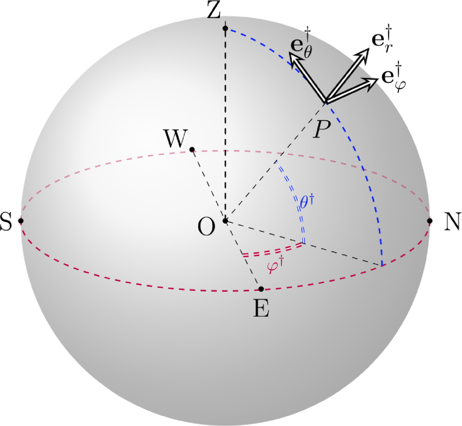
Figure 2.1. Left: classical spherical coordinates. Right: rotated spherical coordinate. Images from [10]. CC BY 4.0 (http://creativecommons.org/licenses/by/4.0)

Away from the boundary layers, the friction/viscous effects are negligible, so the fluid can be considered ideal [9].
The governing equations for a rotating incompressible ideal fluid are, in vectorial coordinate-free form, written as

$$\left\{\begin{aligned} &\frac{D\boldsymbol{u}}{Dt}+2\mathbf{\Omega}\times\boldsymbol{u}+\mathbf{\Omega}\times(\mathbf{\Omega}\times\mathbf{r})=\frac{\mathbf{G}-\nabla p}{\rho},\\ &\frac{D\rho}{Dt}=0,\\ &\nabla\cdot\boldsymbol{u}=0,\end{aligned}\right.$$ (2.8)

where $\frac{D}{Dt}=\left(\frac{\partial}{\partial t}+\boldsymbol{u}\cdot\nabla\right)$ is the material derivative, $\boldsymbol{u}$ is the velocity vector, $\rho$ is the fluid density, $\mathbf{G}$ is the body force per unit volume, $p$ is the pressure, $\mathbf{\Omega}$ the rotation vector and $\mathbf{r}$ the position vector. We anticipate that we will consider three constant densities $\rho_{0}$, $\rho_{1}$ and $\rho_{2}$, with $\rho_{0}<\rho_{1}<\rho_{2}$, in different regions of the flow, therefore the fluid can be considered incompressible.
The three equations in (2.8) correspond to, respectively, the momentum equation, the mass conservation equation, and the incompressibility condition.
In the new rotated spherical coordinates the Euler equations are written as (see [33] for a complete derivation of the Navier-Stokes equations in the rotated spherical coordinate system, from which the incompressible Euler equations reduces to, when considering constant density and zero viscosity)

$$\left[\frac{\partial}{\partial t}+\frac{u^{{\dagger}}}{r\cos\theta^{{\dagger}}}\frac{\partial}{\partial\varphi^{{\dagger}}}+\frac{v^{{\dagger}}}{r}\frac{\partial}{\partial\theta^{{\dagger}}}+w^{{\dagger}}\frac{\partial}{\partial r}\right]\begin{pmatrix}u^{{\dagger}}\\ v^{{\dagger}}\\ w^{{\dagger}}\\ \end{pmatrix}+$$ (2.9)

$$+\frac{1}{r}\begin{pmatrix}-u^{{\dagger}}v^{{\dagger}}\tan\theta^{{\dagger}}+u^{{\dagger}}w^{{\dagger}}\\ u^{{\dagger}2}\tan\theta^{{\dagger}}+v^{{\dagger}}w^{{\dagger}}\\ -u^{{\dagger}2}-v^{{\dagger}2}\end{pmatrix}+2\Omega\begin{pmatrix}-v^{{\dagger}}\sin\varphi^{{\dagger}}\cos\theta^{{\dagger}}-w^{{\dagger}}\sin\varphi^{{\dagger}}\sin\theta^{{\dagger}}\\ u^{{\dagger}}\sin\varphi^{{\dagger}}\cos\theta^{{\dagger}}-w^{{\dagger}}\cos\varphi^{{\dagger}}\\ u^{{\dagger}}\sin\varphi^{{\dagger}}\sin\theta^{{\dagger}}+v^{{\dagger}}\cos\varphi^{{\dagger}}\end{pmatrix}+$$

$$+r\Omega^{2}\begin{pmatrix}\sin\varphi^{{\dagger}}\cos\varphi^{{\dagger}}\cos\theta^{{\dagger}}\\ -\sin^{2}\varphi^{{\dagger}}\sin\theta^{{\dagger}}\cos\theta^{{\dagger}}\\ -\cos^{2}\varphi^{{\dagger}}\cos^{2}\theta^{{\dagger}}-\sin^{2}\theta^{{\dagger}}\end{pmatrix}=-\frac{1}{\rho}\begin{pmatrix}\frac{1}{r\cos\theta^{{\dagger}}}\frac{\partial p}{\partial\varphi^{{\dagger}}}\\ \frac{1}{r}\frac{\partial p}{\partial\theta^{{\dagger}}}\\ \frac{\partial p}{\partial r}\\ \end{pmatrix}-\begin{pmatrix}0\\ 0\\ g\\ \end{pmatrix},$$

and the mass conservation condition

$$\frac{\partial\rho}{\partial t}+\frac{u^{{\dagger}}}{r\cos\theta^{{\dagger}}}\frac{\partial\rho}{\partial\varphi^{{\dagger}}}+\frac{v^{{\dagger}}}{r}\frac{\partial\rho}{\partial\theta^{{\dagger}}}+w^{{\dagger}}\frac{\partial\rho}{\partial r}=0,$$ (2.10)

with $\rho=\rho_{i}$, $i=0,1,2$, depending on region of the flow, and the incompressibility condition is given by

$$\frac{1}{r\cos\theta^{{\dagger}}}\frac{\partial u^{{\dagger}}}{\partial\varphi^{{\dagger}}}+\frac{1}{r}\frac{\partial v^{{\dagger}}}{\partial\theta^{{\dagger}}}-\frac{v^{{\dagger}}}{r}\tan\theta^{{\dagger}}+\frac{\partial w^{{\dagger}}}{\partial r}+\frac{2}{r}w^{{\dagger}}=0.$$ (2.11)

Moreover, as $\mathbf{\Omega}\times(\mathbf{\Omega}\times\mathbf{r})=\frac{1}{2}\nabla(\Omega^{2}\ell^{2})$, where $\ell$ is the distance of the point from the axis of rotation $\mathbf{e}_{3}$, we can redefine the pressure as

$$P=p-\frac{1}{2}\rho\ r^{2}\Omega^{2}(\cos^{2}\varphi^{{\dagger}}\cos^{2}\theta^{{\dagger}}+\sin^{2}\theta^{{\dagger}}).$$ (2.12)

With this redefined pressure, the Euler equations (2.9) read as

$$\left[\frac{\partial}{\partial t}+\frac{u^{{\dagger}}}{r\cos\theta^{{\dagger}}}\frac{\partial}{\partial\varphi^{{\dagger}}}+\frac{v^{{\dagger}}}{r}\frac{\partial}{\partial\theta^{{\dagger}}}+w^{{\dagger}}\frac{\partial}{\partial r}\right]\begin{pmatrix}u^{{\dagger}}\\ v^{{\dagger}}\\ w^{{\dagger}}\\ \end{pmatrix}+\frac{1}{r}\begin{pmatrix}-u^{{\dagger}}v^{{\dagger}}\tan\theta^{{\dagger}}+u^{{\dagger}}w^{{\dagger}}\\ u^{{\dagger}2}\tan\theta^{{\dagger}}+v^{{\dagger}}w^{{\dagger}}\\ -u^{{\dagger}2}-v^{{\dagger}2}\end{pmatrix}$$ (2.13)

$$+2\Omega\begin{pmatrix}-v^{{\dagger}}\sin\varphi^{{\dagger}}\cos\theta^{{\dagger}}-w^{{\dagger}}\sin\varphi^{{\dagger}}\sin\theta^{{\dagger}}\\ u^{{\dagger}}\sin\varphi^{{\dagger}}\cos\theta^{{\dagger}}-w^{{\dagger}}\cos\varphi^{{\dagger}}\\ u^{{\dagger}}\sin\varphi^{{\dagger}}\sin\theta^{{\dagger}}+v^{{\dagger}}\cos\varphi^{{\dagger}}\end{pmatrix}=-\frac{1}{\rho}\begin{pmatrix}\frac{1}{r\cos\theta^{{\dagger}}}\frac{\partial P}{\partial\varphi^{{\dagger}}}\\ \frac{1}{r}\frac{\partial P}{\partial\theta^{{\dagger}}}\\ \frac{\partial P}{\partial r}\\ \end{pmatrix}-\begin{pmatrix}0\\ 0\\ g\\ \end{pmatrix}.$$

2.1. Standard approximations in geophysical fluid dynamics

2.1.1. Tangent plane approximation

Let us start by fixing a point $P$ on the Earth, with rotated spherical coordinates $(\varphi^{{\dagger}}_{0},\theta^{{\dagger}}_{0},R)$ where $R$ is the radius of the Earth. The relation between the coordinates $(X^{{\dagger}},Y^{{\dagger}},Z^{{\dagger}})$ referred to the basis $(\mathbf{e}_{1}^{{\dagger}},\mathbf{e}_{2}^{{\dagger}},\mathbf{e}_{3}^{{\dagger}})$ and rotated spherical coordinates $(\varphi^{{\dagger}},\theta^{{\dagger}},r)$ referred to the basis $(\mathbf{e}_{\varphi}^{{\dagger}},\mathbf{e}_{\theta}^{{\dagger}},\mathbf{e}_{r}^{{\dagger}})$ is given by

$$\left\{\begin{array}[]{ll}X^{{\dagger}}=r\cos\theta^{{\dagger}}\cos\varphi^{{\dagger}},\\ Y^{{\dagger}}=r\cos\theta^{{\dagger}}\sin\varphi^{{\dagger}},\\ Z^{{\dagger}}=r\sin\theta^{{\dagger}}.\end{array}\right.$$ (2.14)

It is well know that the region around $P$ can be approximated by a tangent plane. The sphere of radius $R$ is given by $\mathbf{S}^{2}_{R}=\{(X^{{\dagger}},Y^{{\dagger}},Z^{{\dagger}})\in\mathbb{R}^{3}\,s.t.\,F(X^{{\dagger}},Y^{{\dagger}},Z^{{\dagger}}):=X^{{\dagger}^{2}}+Y^{{\dagger}^{2}}+Z^{{\dagger}^{2}}-R^{2}=0\}$, hence the normal vector to the sphere at $P$ is given by (using (2.14))

$$\boldsymbol{\mathfrak{n}} =\left(\nabla F\right)(P)=2(X_{P}^{{\dagger}},Y_{P}^{{\dagger}},Z_{P}^{{\dagger}})=$$ (2.15)

$$=2R(\cos\theta_{0}\cos\varphi_{0},\,\cos\theta_{0}\sin\varphi_{0},\,\sin\theta_{0}).$$

The vector $\boldsymbol{\mathfrak{n}}$ is (up to normalizing) equal to the base vector $\mathbf{e}_{r}^{{\dagger}}(P)$ (see equation (2.7)), and, since the tangent plane to the sphere at the point $P$ is the geometric locus of points $M$ such that $\vec{PM}\cdot\boldsymbol{\mathfrak{n}}=\vec{PM}\cdot\mathbf{e}_{r}(P)=0$, it’s an immediate consequence that a basis for the tangent plane at $P$ is $(\mathbf{e}_{\varphi}^{{\dagger}}(P),\mathbf{e}_{\theta}^{{\dagger}}(P))$.
On the tangent plane we define the following local coordinates

$$\left\{\begin{aligned} &\mathsf{x}=R\cos\theta^{{\dagger}}_{0}(\varphi^{{\dagger}}-\varphi^{{\dagger}}_{0}),\\ &\mathsf{y}=R(\theta^{{\dagger}}-\theta^{{\dagger}}_{0}),\\ \end{aligned}\right.$$ (2.16)

therefore, computing

$$\nabla\mathsf{x}=R\cos\theta^{{\dagger}}_{0}\ \mathbf{e}_{\varphi}^{{\dagger}}(P),\\ \qquad\nabla\mathsf{y}=R\ \mathbf{e}_{\theta}^{{\dagger}}(P),$$ (2.17)

we obtain the following basis

$$\mathbf{e}_{\mathsf{x}}=\frac{\nabla\mathsf{x}}{|\nabla\mathsf{x}|}=\mathbf{e}_{\varphi}(P),\qquad\mathbf{e}_{\mathsf{y}}=\frac{\nabla\mathsf{y}}{|\nabla\mathsf{y}|}=\mathbf{e}_{\theta}(P),$$ (2.18)

proving that $(\mathbf{e}_{\varphi}^{{\dagger}}(P),\mathbf{e}_{\theta}^{{\dagger}}(P))$ is in fact a basis for the tangent plane at $P$.
The concept of tangent plane is always used implicitly for the horizontal variables when adopting a $f$-plane approximation.
The partial derivatives with respect to $(\mathsf{x},\mathsf{y})$ are given by

$$\frac{\partial}{\partial\mathsf{x}}=\frac{1}{R\cos\theta_{0}}\frac{\partial}{\partial\varphi^{{\dagger}}},\qquad\frac{\partial}{\partial\mathsf{y}}=\frac{1}{R}\frac{\partial}{\partial\theta^{{\dagger}}}.$$ (2.19)

2.1.2. Traditional approximation

In this paragraph we review the ideas leading to the so-called traditional approximation, adapting them to the rotated spherical coordinates. Namely, we will construct this approximation starting from (2.13). Note that, even if the velocities $u^{{\dagger}},v^{{\dagger}},w^{{\dagger}}$ are defined differently from the ones relative to the classical spherical coordinate system, $u^{{\dagger}},v^{{\dagger}}$ are still the horizontal and $w^{{\dagger}}$ the vertical components of the velocity vector $\boldsymbol{u}$, hence the observations about their magnitude, on which the traditional approximation is bases, still apply.
For a review of the traditional approximation of the governing equations in classical spherical coordinates we refer to [39] and [23].
The first step involves neglecting metric terms

$$\frac{1}{r}\left(-u^{{\dagger}}v^{{\dagger}}\tan\theta^{{\dagger}}+u^{{\dagger}}w^{{\dagger}},\,u^{{\dagger}2}\tan\theta^{{\dagger}}+v^{{\dagger}}w^{{\dagger}},\,-u^{{\dagger}2}-v^{{\dagger}2}\right),$$ (2.20)

which represent the effect of curvature in spherical coordinates, in (2.13), and the terms in (2.10) and (2.11) which involves a velocity multiplied by $\frac{1}{r}$. Because of the thinnes of the atmosphere and ocean, vertical velocities (typically $\leq 0.01\,\mathrm{ms^{-1}}$) are much less than horizontal velocities by a factor of $10^{-4}$ on average, therefore we may neglect the term involving $w^{{\dagger}}$ in the horizontal components (namely the first two) of the Coriolis acceleration

$$2\mathbf{\Omega}\times\mathbf{u}=2\Omega\begin{pmatrix}-v^{{\dagger}}\sin\varphi^{{\dagger}}\cos\theta^{{\dagger}}-w^{{\dagger}}\sin\varphi^{{\dagger}}\sin\theta^{{\dagger}}\\ u^{{\dagger}}\sin\varphi^{{\dagger}}\cos\theta^{{\dagger}}-w^{{\dagger}}\cos\varphi^{{\dagger}}\\ u^{{\dagger}}\sin\varphi^{{\dagger}}\sin\theta^{{\dagger}}+v^{{\dagger}}\cos\varphi^{{\dagger}}\end{pmatrix}.$$ (2.21)

Moreover, in the atmosphere the typical scale of the horizontal velocities is $|u^{{\dagger}}|,\,|v^{{\dagger}}|\approx 10\,\mathrm{ms^{-1}}$, and even less in the ocean, giving that $|2\Omega(u^{{\dagger}}+v^{{\dagger}})|\approx 3\cdot 10^{-3}\,\mathrm{ms^{-2}}$, is negligible compared to gravity acceleration $g\approx 9.8\,\mathrm{ms^{-2}}$. Therefore, the Coriolis acceleration can be approximated as

$$2\mathbf{\Omega}\times\mathbf{u}\approx 2\Omega\begin{pmatrix}-v^{{\dagger}}\sin\varphi^{{\dagger}}\cos\theta^{{\dagger}}\\ u^{{\dagger}}\sin\varphi^{{\dagger}}\cos\theta^{{\dagger}}\\ 0\end{pmatrix}.$$ (2.22)

These two approximations related to the Coriolis term $2\mathbf{\Omega}\times\mathbf{u}$, the first involving the two horizontal components of the equation, and the second involving the vertical component where the gravity acceleration is present, cannot be done independently of each other. Instead, they must be made together, otherwise the resulting equations fail to conserve energy [35].
Lastly, as the ocean is shallow compared to Earth’s radius, we can write $r=R+\mathsf{z}$, with $R$ being the Earth’s radius and $\mathsf{z}$ increasing in the radial direction. This idea is fundamental for the so-called ‘thin-shell’ approximation (see e.g [10]). The coordinate $r$ is then replaced by $R$, except in the derivatives. For example $\frac{1}{r^{2}}\frac{\partial r^{2}w^{{\dagger}}}{\partial r}$ becomes $\frac{\partial w^{{\dagger}}}{\partial\mathsf{z}}$. With the above arguments, the Euler, mass conservation and incompressibility equations reduces to

$$\left\{\begin{aligned} &\left[\frac{\partial}{\partial t}+\frac{u^{{\dagger}}}{R\cos\theta^{{\dagger}}}\frac{\partial}{\partial\varphi^{{\dagger}}}+\frac{v^{{\dagger}}}{R}\frac{\partial}{\partial\theta^{{\dagger}}}+w^{{\dagger}}\frac{\partial}{\partial\mathsf{z}}\right]\begin{pmatrix}u^{{\dagger}}\\ v^{{\dagger}}\\ w^{{\dagger}}\\ \end{pmatrix}+\\ &\qquad+2\Omega\begin{pmatrix}-v^{{\dagger}}\sin\varphi^{{\dagger}}\cos\theta^{{\dagger}}\\ u^{{\dagger}}\sin\varphi^{{\dagger}}\cos\theta^{{\dagger}}\\ 0\end{pmatrix}=-\frac{1}{\rho}\begin{pmatrix}\frac{1}{R\cos\theta^{{\dagger}}}\frac{\partial P}{\partial\varphi^{{\dagger}}}\\ \frac{1}{R}\frac{\partial P}{\partial\theta^{{\dagger}}}\\ \frac{\partial P}{\partial\mathsf{z}}\\ \end{pmatrix}-\begin{pmatrix}0\\ 0\\ g\\ \end{pmatrix}\\ &\,\frac{\partial\rho}{\partial t}+\frac{u^{{\dagger}}}{R\cos\theta^{{\dagger}}}\frac{\partial\rho}{\partial\varphi^{{\dagger}}}+\frac{v^{{\dagger}}}{R}\frac{\partial\rho}{\partial\theta^{{\dagger}}}+w^{{\dagger}}\frac{\partial\rho}{\partial\mathsf{z}}=0\\ &\,\frac{1}{R\cos\theta^{{\dagger}}}\frac{\partial u^{{\dagger}}}{\partial\varphi^{{\dagger}}}+\frac{1}{R}\frac{\partial v^{{\dagger}}}{\partial\theta^{{\dagger}}}+\frac{\partial w^{{\dagger}}}{\partial\mathsf{z}}=0,\end{aligned}\right.$$ (2.23)

respectively.

2.1.3. $f$-plane approximation in the rotated spherical coordinates framework

Usually, the Coriolis parameter is defined by $f=2\Omega\sin\theta$, where $\theta\in\left[-\frac{\pi}{2},\frac{\pi}{2}\right]$ is the classical angle of latitidue (see [27]), but, due to the relation $\sin\theta=\cos\theta^{{\dagger}}\sin\varphi^{{\dagger}}$ in (2.5) we can write

$$f=2\Omega\sin\theta=2\Omega\cos\theta^{{\dagger}}\sin\varphi^{{\dagger}},$$ (2.24)

and it follows that

$$\frac{\partial f}{\partial\varphi^{{\dagger}}}=2\Omega\cos\theta^{{\dagger}}\cos\varphi^{{\dagger}},\qquad\frac{\partial f}{\partial\varphi^{{\dagger}}}=-2\Omega\sin\theta^{{\dagger}}\sin\varphi^{{\dagger}}.$$

Using a Taylor expansion at the firts order, we can write

$$f =f_{0}+\frac{\partial f(\varphi_{0}^{{\dagger}},\theta^{{\dagger}}_{0})}{\partial\varphi^{{\dagger}}}\left(\varphi^{{\dagger}}-\varphi^{{\dagger}}_{0}\right)+\frac{\partial f(\varphi_{0}^{{\dagger}},\theta^{{\dagger}}_{0})}{\partial\varphi^{{\dagger}}}\left(\theta^{{\dagger}}-\theta^{{\dagger}}_{0}\right)+\mathcal{O}\left(\varphi^{{\dagger}^{2}},\theta^{{\dagger}^{2}}\right)=$$ (2.25)

$$=f_{0}+\mathcal{O}\left(\varphi^{{\dagger}},\theta^{{\dagger}}\right),$$

where $f_{0}=2\Omega\cos\theta_{0}^{{\dagger}}\sin\varphi_{0}^{{\dagger}}$.
As described previously, in the rotated spherical coordinates framework, a small region around a specific point of coordinates $\theta^{{\dagger}}_{0},\varphi^{{\dagger}}_{0},R$, can be described by taking a tangent plane approximation (for the horizontal coordinates), given by (2.16)

$$\left\{\begin{aligned} &\mathsf{x}=R\cos\theta^{{\dagger}}_{0}(\varphi^{{\dagger}}-\varphi^{{\dagger}}_{0}),\\ &\mathsf{y}=R(\theta^{{\dagger}}-\theta^{{\dagger}}_{0}),\\ \end{aligned}\right.$$ (2.26)

so that the $\mathsf{x}$-axis points toward the North Pole, the $\mathsf{y}$-axis points toward the Null Island, while the vertical $\mathsf{z}$-axis is assume to point upward. As for the classical $f$-plane approximation, the Coriolis parameter $f$ is assumed to remain constant and equal to $f_{0}$ within the localized region. As an $f$-plane approximation is implicitly based on a tangent plane approximation, the error committed by adopting this approximation is of order of $\mathcal{O}\left(\frac{\mathsf{x}}{R},\frac{\mathsf{y}}{R}\right).$
The Euler, mass conservation and incompressibility equations in the $f$-plane approximation are given by

$$\left\{\begin{aligned} &\left[\frac{\partial}{\partial t}+u^{{\dagger}}\frac{\partial}{\partial\mathsf{x}}+v^{{\dagger}}\frac{\partial}{\partial\mathsf{y}}+w^{{\dagger}}\frac{\partial}{\partial\mathsf{z}}\right]\begin{pmatrix}u^{{\dagger}}\\ v^{{\dagger}}\\ w^{{\dagger}}\\ \end{pmatrix}+\begin{pmatrix}-fv^{{\dagger}}\\ fu^{{\dagger}}\\ 0\end{pmatrix}=-\frac{1}{\rho}\begin{pmatrix}\frac{\partial P}{\partial\mathsf{x}}\\ \frac{\partial P}{\partial\mathsf{y}}\\ \frac{\partial P}{\partial\mathsf{z}}\\ \end{pmatrix}-\begin{pmatrix}0\\ 0\\ g\\ \end{pmatrix},\\ &\frac{\partial\rho}{\partial t}+u^{{\dagger}}\frac{\partial\rho}{\partial\mathsf{x}}+v^{{\dagger}}\frac{\partial\rho}{\partial\mathsf{y}}+w^{{\dagger}}\frac{\partial\rho}{\partial\mathsf{z}}=0,\\ &\frac{\partial u^{{\dagger}}}{\partial\mathsf{x}}+\frac{\partial v^{{\dagger}}}{\partial\mathsf{y}}+\frac{\partial w^{{\dagger}}}{\partial\mathsf{z}}=0.\end{aligned}\right.$$ (2.27)

These equations hold for general $\rho=\rho(x,y,z)$, but, as anticipated, we will consider three constant densities $\rho_{0},\ \rho_{1},\ \rho_{2}$; consequently the mass conservation equation (namely the second of (2.27)) will always satisfied.

2.2. North Pole and coordinates relative to the TDC

The use of the newly defined, rotated spherical coordinates $(\varphi^{{\dagger}},\theta^{{\dagger}},r)$, along with the corresponding governing equations, is particularly applicable when analyzing flows in regions centered at the poles, where standard spherical coordinates are not defined.
Our analysis focus on a region centered at the North Pole, having coordinates $\varphi^{{\dagger}}_{0}=\frac{\pi}{2},\ \theta^{{\dagger}}_{0}=0$ (and $r=R$). This imply that $f_{0}=2\Omega$ and the tangent plane coordinates are given by

$$\left\{\begin{aligned} &\mathsf{x}=R\left(\varphi^{{\dagger}}-\frac{\pi}{2}\right),\\ &\mathsf{y}=R\theta^{{\dagger}},\\ \end{aligned}\right.$$ (2.28)

with basis given by $\mathbf{e}_{\varphi}^{{\dagger}}(\mathfrak{N}),\mathbf{e}_{\theta}^{{\dagger}}((\mathfrak{N}))$, with $\mathfrak{N}$ representing the North Pole. See Figure 2.2 for a depiction of the basis at the North Pole.

Figure 2.2. Depiction of the basis at North Pole. In reality, the angle $\gamma$ is bigger than the one depicted here (close to $90^{\circ}$). However, for graphical clarity reason we did is smaller ($70^{\circ}).$

The last step involves defining a new basis $\mathbf{e}_{x},\mathbf{e}_{y}$ for the tangent plane, by simply rotating anticlockwise the basis $\mathbf{e}_{\varphi}^{{\dagger}}(\mathfrak{N}),\mathbf{e}_{\theta}^{{\dagger}}((\mathfrak{N}))$ of a certain angle $\gamma$, in order to align the first basis vector with the Transpolar Drift Current (this angle would be around $80^{\circ}$ or even $90^{\circ}$).
These unit vectors are given by (see Figure 2.2)

$$\left\{\begin{aligned} &\mathbf{e}_{x}=\cos\gamma\mathbf{e}_{\varphi}^{{\dagger}}(\mathfrak{N})+\sin\gamma\mathbf{e}_{\theta}^{{\dagger}}((\mathfrak{N})),\\ &\mathbf{e}_{y}=-\sin\gamma\mathbf{e}_{\varphi}^{{\dagger}}(\mathfrak{N})+\cos\gamma\mathbf{e}_{\theta}^{{\dagger}}((\mathfrak{N})).\end{aligned}\right.$$ (2.29)

Finally, observe that, as $\mathbf{\Omega}\times(\mathbf{\Omega}\times\mathbf{r})=\frac{1}{2}\nabla(\Omega^{2}\ell^{2})$ where $\ell$ is the distance from the axis of rotation $\mathbf{e}_{3}$, this will not change when adopting this new basis, hence there is no need to modify the expression for the pressure (2.12).
The governing equations with respect to the new basis are therefore given by

$$\left\{\begin{aligned} &\frac{\partial u}{\partial t}+u\frac{\partial u}{\partial x}+v\frac{\partial u}{\partial y}+w\frac{\partial u}{\partial z}-fv=-\frac{1}{\rho}\frac{\partial P}{\partial x},\\ &\frac{\partial v}{\partial t}+u\frac{\partial v}{\partial x}+v\frac{\partial v}{\partial y}+w\frac{\partial v}{\partial z}+fu=-\frac{1}{\rho}\frac{\partial P}{\partial y},\\ &\frac{\partial w}{\partial t}+u\frac{\partial w}{\partial x}+v\frac{\partial w}{\partial y}+w\frac{\partial w}{\partial z}+g=-\frac{1}{\rho}\frac{\partial P}{\partial z},\end{aligned}\right.$$ (2.30)

$$\frac{\partial u}{\partial x}+\frac{\partial v}{\partial y}+\frac{\partial w}{\partial z}=0,$$ (2.31)

where $(u,v,w)$ are the velocity component associated to the basis $\left(\mathbf{e}_{x},\mathbf{e}_{y},\mathbf{e}_{r}(\mathfrak{N})\right)$, and with $\rho$ equal $\rho_{0},\ \rho_{1}$ or $\rho_{2}$ depending on the layer of the fluid we are considering.
For consistency of notation we have used $z$ in place of $\mathsf{z}$.

3. Description of flows

The simplified model we are considering features three constant densities, $\rho_{0}$, $\rho_{1}$ and $\rho_{2}$, characterizing the three strata, with $\rho_{0}<\rho_{1}<\rho_{2}$. The fresh and cold water of the surface mixed layer above the halocline has density $\rho_{0}$, $\rho_{1}$ is the density of the halocline’s water and $\rho_{2}$ is the density of the saltier and warmer water Atlantic Water below the halocline. As depth increases, the surface turbulent effect tend to vanish, even more with the presence of ice, so we may assume that just above the lower boundary of the SML, that we denote by $\eta_{1}$, there exist a layer (eventually this) where the fluid flows in the direction of the TDC with uniform constant speed $\mathsf{c}\approx 0.1\,\mathrm{ms^{-1}}$. We indicate the upper boundary of this eventually thin layer $\eta_{0}$, but as will be evident from our solution, the particular expression of $\eta$ doesn’t affect our analysis. Moreover, we assume the layer under the halocline to be practically motionless, and we denote by $\eta_{2}$ the lower surface of the halocline.
In addition to the governing equations (2.30) and (2.31) we require the solution to satisfy the dynamic boundary condition (i.e. the pressure must be continuous across the surfaces $\eta_{1}$ and $\eta_{2}$), and the kinematic boundary condition

$$w=\frac{\partial\eta_{i}}{\partial t}+u\frac{\partial\eta_{i}}{\partial x}+v\frac{\partial\eta_{i}}{\partial y}\quad\text{on}\ z=\eta_{i},\quad i=1,2,$$ (3.1)

preventing the mixing of fluid particles between different layers (see [5]).
Due to their different character, we will describe the flow in each layer separately

3.1. The thin uniform layer above $\eta_{1}$

In the region $\eta_{1}(x-\mathsf{c}t,y)<z<\eta_{0}(x-\mathsf{c}t,y)$ , we set the density $\rho=\rho_{0}$ and we assume the flow to be uniform: $u=\mathsf{c},\ v=w=0$. The Euler equations (2.30) therefore simplifies to

$$\left\{\begin{aligned} &\frac{\partial P}{\partial x}=0,\\ &\frac{\partial P}{\partial y}=-\rho_{0}f\mathsf{c},\\ &\frac{\partial P}{\partial z}=-\rho_{0}g,\end{aligned}\right.$$ (3.2)

leading to the following expression for the pressure:

$$P(x,y,z)=P_{0}-\rho_{0}gz-\rho_{0}f\mathsf{c}y,$$ (3.3)

where $f=2\Omega\approx 1.5\cdot 10^{-4}\,\mathrm{s^{-1}}$ and $P_{0}\in\mathbb{R}$.
It is immediate to show that the uniform flow $u=\mathsf{c},\ v=w=0$ satisfies the continuity equation (2.31), and that the flow in irrotational in the layer above $\eta_{1}$, as the vorticity vector

$$\omega=\left(\frac{\partial w}{\partial y}-\frac{\partial v}{\partial z},\frac{\partial u}{\partial z}-\frac{\partial w}{\partial x},\frac{\partial v}{\partial x}-\frac{\partial u}{\partial y}\right)=(0,0,0).$$ (3.4)

3.2. The deep motionless layer beneath the halocline

In the region $z<\eta_{2}(x-\mathsf{c}t,y)$ the water is in hydrostatic state $u=v=w=0$, hence (2.30) reads as

$$\left\{\begin{aligned} &\frac{\partial P}{\partial x}=0,\\ &\frac{\partial P}{\partial y}=0,\\ &\frac{\partial P}{\partial z}=-\rho_{2}g,\end{aligned}\right.$$ (3.5)

giving, for the pressure,

$$P(x,y,z)=P_{2}-\rho_{2}gz,$$ (3.6)

with $P_{2}\in\mathbb{R}$. Being hydrostatic, the flow is irrotational (i.e. (3.4) holds) and solves the continuity equation (2.31).

3.3. The halocline layer $\eta_{2}\leq z\leq\eta_{1}$

In contrast to the layers analyzed before, we seek an explicit solution of (2.30), (2.31) and (3.1), fulfilling also the dynamic boundary condition, in the Lagrangian formalism (see [1] for a review): at time $t$ we specify the positions of the fluid particles in terms of the labeling variables $(q,\ r,\ s)$ by

$$\left\{\begin{aligned} &x=q-be^{-ms}\sin(k(q-\mathsf{c}t)),\\ &y=r-de^{-ms}\cos(k(q-\mathsf{c}t)),\\ &z=-d_{0}+s-ae^{-ms}\cos(k(q-\mathsf{c}t)).\end{aligned}\right.$$ (3.7)

The constant $k=\frac{2\pi}{L}>0$ is the wave number corresponding to the wavelength $L$, and we assume $m>0$ and $a>0$, while the labeling variables are chosen so that

$$(q,r,s)\in\mathbb{R}\times[-\mathrm{r}_{0},\mathrm{r}_{0}]\times[\mathrm{s}_{-}(r),\mathrm{s}_{+}(r)],$$ (3.8)

where $s=\mathrm{s}_{-}(r)\geq\mathrm{s}^{*}>0$ represents $\eta_{2}$, $s=\mathrm{s}_{+}(r)>\mathrm{s}_{-}(r)$ represents $\eta_{1}$ and $\mathrm{r}_{0}=\mathrm{c}_{0}/f\approx 15\,Km$ is the baroclinic radius of deformation ($\mathrm{c}_{0}\approx 2.2m/s$ is the baroclinic gravity wave speed at the North Pole; (see [17] or [28]), and $d_{0}-\mathrm{s_{-}}$ is the mean depth of the halocline base.
It will be shown that (3.7), representing waves with crests parallel to the $y$-axis and propagating in the direction of the $x$-axis, is a solution of the Euler and incompressibility equations.
The particle motion in (3.7) describes trochoidal orbits, namely the path of a fixed point on a circle of radius $be^{-ms}$ and centered at $(q,r,s-d_{0})$, rolling along the $x$-axis, in a plane that is at an angle $\arctan(-d/a)$ with respect to the vertical axis.
Anticipating the relation $a^{2}+d^{2}=b^{2}$, cf. (3.31), and recalling that a circle in three dimension in uniquely defined by six numbers (three for the circle’s center, one for the radius and two for the orientation of the unit vector normal to the plane of the circle), namely:

$$\mathrm{circle}=\left\{\mathbf{C}+\mathcal{R}\cos{\theta}\boldsymbol{\mu}+\mathcal{R}\cos{\theta}\boldsymbol{\nu}\times\boldsymbol{\mu}\right\}_{\theta\in[0,2\pi)},$$ (3.9)

where $\mathbf{C}$ is the center of the circle, $\mathcal{R}$ its radius, $\boldsymbol{\nu}$ is the unit vector normal to the plane of the circle, $\boldsymbol{\mu}$ is a vector orthogonal to $\boldsymbol{\nu}$ and $\theta$ is the angular position on the circle, it is immediate to see that we recover (3.7) by setting

$$\mathbf{C}=(q,r,s-d_{0}),\qquad\mathcal{R}=be^{-ms},\qquad\theta=\tau=k(q-\mathsf{c}t),$$ (3.10)

$$\boldsymbol{\nu}=\left(0,\frac{a}{b},\frac{-d}{b}\right),\qquad\boldsymbol{\mu}=\left(0,\frac{-d}{b},\frac{a}{b}\right),$$

The Jacobian of the map (3.7) relating the particle positions with the Lagrangian labeling variables is given by

$$\left(\frac{\partial(x,y,z)}{\partial(q,r,s)}\right) =\begin{pmatrix}\frac{\partial x}{\partial q}&\frac{\partial y}{\partial q}&\frac{\partial z}{\partial q}\\ \frac{\partial x}{\partial r}&\frac{\partial y}{\partial r}&\frac{\partial z}{\partial r}\\ \frac{\partial x}{\partial s}&\frac{\partial y}{\partial s}&\frac{\partial z}{\partial s}\par\end{pmatrix}=$$ (3.11)

$$=\begin{pmatrix}1-kbe^{-ms}\cos\tau&kde^{-ms}\sin\tau&kae^{-ms}\sin\tau\\ 0&1&0\\ mbe^{-ms}\sin\tau&mde^{-ms}\cos\tau&1+mae^{-ms}\cos\tau\end{pmatrix},$$

with

$$\tau=k(q-\mathsf{c}t),$$ (3.12)

and its determinant is expressed by

$$J=1+(am-bk)e^{-ms}\cos\tau-kmab\,e^{-2ms}.$$ (3.13)

The flow is incompressible, namely (2.31) holds, if $J$ is time-independent and non-zero, giving

$$am=bk,$$ (3.14)

thus providing

$$J=1-m^{2}a^{2}\,e^{-2ms}\not=0.$$ (3.15)

The above condition that $J\not=0$ implies that (3.7) is a local diffeomorphic change of coordinates by the inverse function theorem. Since $s\geq\mathrm{s}^{*}>0$,

$$a^{2}m^{2}\,e^{-2m\mathrm{s}^{*}}<1,$$ (3.16)

and, as $ae^{-m\mathrm{s}^{*}}$ is the amplitude of a wave at some $r$, it is possible to find an upper bound for the vertical amplitude:

$$a_{\mathrm{max}}=\frac{1}{m}.$$ (3.17)

Morevoer, due to (3.16), it is evident that

$$J=1-m^{2}a^{2}\,e^{-2ms}>0.$$ (3.18)

The velocity and acceleration of a particle can be computed using (3.7), giving respectively

$$\left\{\begin{aligned} &u=\frac{Dx}{Dt}=k\mathsf{c}b\,e^{-ms}\cos\tau,\\ &v=\frac{Dy}{Dt}=-k\mathsf{c}d\,e^{-ms}\sin\tau,\\ &w=\frac{Dz}{Dt}=-k\mathsf{c}a\,e^{-ms}\sin\tau,\end{aligned}\right.\qquad\text{and}\qquad\left\{\begin{aligned} &\frac{Du}{Dt}=k^{2}\mathsf{c}^{2}b\,e^{-ms}\sin\tau,\\ &\frac{Dv}{Dt}=k^{2}\mathsf{c}^{2}d\,e^{-ms}\cos\tau,\\ &\frac{Dw}{Dt}=k^{2}\mathsf{c}^{2}a\,e^{-ms}\cos\tau,\end{aligned}\right.$$ (3.19)

therefore, the Euler equations (2.30) rewritten in a more compact form as

$$\left\{\begin{aligned} &\frac{\partial P}{\partial x}=-\rho_{1}\left[\frac{Du}{Dt}-fv\right],\\ &\frac{\partial P}{\partial y}=-\rho_{1}\left[\frac{Dv}{Dt}+fu\right],\\ &\frac{\partial P}{\partial z}=-\rho_{1}\left[\frac{Dw}{Dt}+g\right],\\ \end{aligned}\right.$$ (3.20)

lead to

$$\left\{\begin{aligned} &\frac{\partial P}{\partial x}=-\rho_{1}\,e^{-ms}\sin\tau\left[k^{2}\mathsf{c}^{2}b+k\mathsf{c}df\right],\\ &\frac{\partial P}{\partial y}=-\rho_{1}\,e^{-ms}\cos\tau\left[k^{2}\mathsf{c}^{2}d+k\mathsf{c}bf\right],\\ &\frac{\partial P}{\partial z}=--\rho_{1}\,e^{-ms}\left[k^{2}\mathsf{c}^{2}a\,e^{-ms}\cos\tau+g\right].\\ \end{aligned}\right.$$ (3.21)

Given (3.21), the pressure gradient with respect to the Lagrangian labeling variables is given by

$$\begin{pmatrix}\frac{\partial P}{\partial q}\\ \frac{\partial P}{\partial r}\\ \frac{\partial P}{\partial s}\end{pmatrix}=\begin{pmatrix}\frac{\partial x}{\partial q}&\frac{\partial y}{\partial q}&\frac{\partial z}{\partial q}\\ \frac{\partial x}{\partial r}&\frac{\partial y}{\partial r}&\frac{\partial z}{\partial r}\\ \frac{\partial x}{\partial s}&\frac{\partial y}{\partial s}&\frac{\partial z}{\partial s}\end{pmatrix}\begin{pmatrix}\frac{\partial P}{\partial x}\\ \frac{\partial P}{\partial y}\\ \frac{\partial P}{\partial z}\\ \end{pmatrix},$$ (3.22)

providing

$$\left\{\begin{aligned} &\frac{\partial P}{\partial q}=-\rho_{1}\left\{k^{3}\mathsf{c}^{2}(a^{2}+d^{2}-b^{2})e^{-2ms}\cos\tau\sin\tau+(bk^{2}\mathsf{c}^{2}+dkf\mathsf{c}+gak)e^{-ms}\sin\tau\right\},\\ &\frac{\partial P}{\partial r}=-\rho_{1}\left\{k\mathsf{c}(k\mathsf{c}d+fb)e^{-ms}\cos\tau\right\},\\ &\frac{\partial P}{\partial s}=-\rho_{1}\left\{mk^{2}\mathsf{c}^{2}(a^{2}+d^{2}-b^{2})e^{-2ms}\cos^{2}\tau\right.+\\ &\qquad\qquad\left.+(ak^{2}\mathsf{c}^{2}+gam)e^{-ms}\cos\tau+mk\mathsf{c}(k\mathsf{c}b^{2}+fbd)e^{-2ms}+g\right\}.\end{aligned}\right.$$ (3.23)

In order to find other two relations for $a,b,d,k,m,\mathsf{c},f$, we require the pressure to have continuous second-order partial derivatives (at least in the halocline layer), giving

$$\frac{\partial^{2}P}{\partial q\partial r}=\frac{\partial^{2}P}{\partial r\partial q}\Rightarrow k\mathsf{c}d+fb=0,$$ (3.24)

$$\frac{\partial^{2}P}{\partial q\partial s}=\frac{\partial^{2}P}{\partial s\partial q}\Rightarrow mk\mathsf{c}^{2}b+m\mathsf{c}df=k^{2}\mathsf{c}^{2}a.$$ (3.25)

Moreover, as a consequence of (3.24) we have that

$$\frac{\partial P}{\partial r}=0.$$ (3.26)

Therefore, for every constant $P_{1}$, the gradient of

$$P(q-\mathsf{c}t,r,s)=$$ (3.27)

$$=P_{1}-\rho_{1}gs+\frac{\rho_{1}}{2}(b^{2}k^{2}\mathsf{c}^{2}+fbdk\mathsf{c})e^{-2ms}+$$

$$\ +\rho_{1}(bk\mathsf{c}^{2}+df\mathsf{c}+ga)e^{-ms}\cos\tau+\frac{\rho_{1}}{2}k^{2}\mathsf{c}^{2}(a^{2}+d^{2}-b^{2})e^{-2ms}\cos^{2}\tau$$

with respect to the the labeling variables $(q,s,r)$ gives the right-hand side of (3.23).
Let us rewrite the relations (3.14), (3.24) and (3.25) as

$$b=\frac{ma}{k},$$ (3.28)

$$d=-\frac{fma}{k^{2}\mathsf{c}},$$ (3.29)

$$m^{2}=\frac{k^{4}\mathsf{c}^{2}}{k^{2}\mathsf{c}^{2}-f^{2}},$$ (3.30)

Observe that (3.28), (3.29) and (3.30) give also the relation

$$a^{2}+d^{2}=b^{2},$$ (3.31)

and (3.27) reduces to

$$P(q-\mathsf{c}t,r,s)=P_{1}-\rho_{1}gs +\frac{\rho_{1}}{2}(b^{2}k^{2}\mathsf{c}^{2}+fbdk\mathsf{c})e^{-2ms}+$$ (3.32)

$$\ +\rho_{1}(bk\mathsf{c}^{2}+df\mathsf{c}+ga)e^{-ms}\cos\tau$$

The dispersion relation and the expression for the wavenumber $k=\frac{2\pi}{L}$ will be provided imposing the dynamic boundary condition across the surfaces $\eta_{1}$ and $\eta_{2}$.

3.3.1. The upper surface of the halocline $\eta_{1}$

For every $r\in[-\mathrm{r}_{0},\mathrm{r}_{0}]$, the upper surface of the halocline $\eta_{1}$ is described by $s=\mathrm{s}_{+}(r)$, and the continuity of the pressure is imposed by equaling (3.32) and (3.3) at $s=\mathrm{s}_{+}(r)$:

$$P_{0}-\rho_{0}g(-d_{0}+\mathrm{s}_{+}-ae^{-m\mathrm{s}_{+}}\cos\tau)-\rho_{0}f\mathsf{c}(r-de^{-m\mathrm{s}_{+}}\cos\tau)=$$ (3.33)

$$=P_{1}-\rho_{1}g\mathrm{s}_{+}+\frac{\rho_{1}}{2}(b^{2}k^{2}\mathsf{c}^{2}+fbdk\mathsf{c})e^{-2m\mathrm{s}_{+}}+\rho_{1}(bk\mathsf{c}^{2}+df\mathsf{c}+ga)e^{-m\mathrm{s}_{+}}\cos\tau.$$

Equation (3.33) is satisfied if

$$\left\{\begin{aligned} &P_{0}-P_{1}=\frac{1}{2}\rho_{1}bk\mathsf{c}(bk\mathsf{c}+df)e^{-2m\mathrm{s}_{+}}-(\rho_{1}-\rho_{0})g\mathrm{s}_{+}+\rho_{0}f\mathsf{c}r-\rho_{0}gd_{0},\\ &bk\mathsf{c}^{2}=\left(\frac{\rho_{0}-\rho_{1}}{\rho_{1}}\right)(ga+f\mathsf{c}d),\end{aligned}\right.$$ (3.34)

therefore $\eta_{1}$ is determined by setting $s=\mathrm{s}_{+}(r)$ at a fixed value of $r\in[-\mathrm{r}_{0},\mathrm{r}_{0}]$, where $\mathrm{s}_{+}(r)$ is the unique solution of

$$P_{0}-P_{1}=\frac{1}{2}\rho_{1}bk\mathsf{c}(bk\mathsf{c}+df)e^{-2ms}-(\rho_{1}-\rho_{0})gs+\rho_{0}f\mathsf{c}r-\rho_{0}gd_{0}.$$ (3.35)

For every fixed $r\in[-\mathrm{r}_{0},\mathrm{r}_{0}]$, the function

$$s\longmapsto\frac{\rho_{1}}{2}(b^{2}k^{2}\mathsf{c}^{2}+bk\mathsf{c}df)e^{-2ms}-(\rho_{1}-\rho_{0})gs,$$ (3.36)

is a strictly decreasing diffeomorphism from $(0,+\infty)$ to $(-\infty,A)$, where $A=\frac{1}{2}\rho_{1}(b^{2}k^{2}\mathsf{c}^{2}+bk\mathsf{c}df)$. Consequently, by the implicit function theorem, if

$$P_{0}-P_{1}-\rho_{0}f\mathsf{c}r+\rho_{0}gd_{0}<A,$$ (3.37)

for every fixed $r\in[-\mathrm{r}_{0},\mathrm{r}_{0}]$, we can find a unique (smooth) solution $\mathrm{s}_{+}(r)>0$ of (3.35). Note that

$$A =\frac{1}{2}\rho_{1}(b^{2}k^{2}\mathsf{c}^{2}+bk\mathsf{c}df)=\frac{1}{2}\rho_{1}m^{2}a^{2}\left(\mathsf{c}^{2}-\frac{f^{2}}{k^{2}}\right)=$$ (3.38)

$$=\frac{1}{2}\rho_{1}a^{2}\frac{k^{4}\mathsf{c}^{2}}{k^{2}\mathsf{c}^{2}-f^{2}}\frac{k^{2}\mathsf{c}^{2}-f^{2}}{k^{2}}=\frac{1}{2}\rho_{1}a^{2}k^{2}\mathsf{c}^{2}>0,$$

where we used (3.28), (3.29) and (3.30).
Evaluating (3.35) at $s=\mathrm{s}_{+}(r)$ and differentiating with respect to $r$ gives

$$\mathrm{s}^{\prime}_{+}(r)=\frac{\rho_{0}f\mathsf{c}}{2mAe^{-2m\mathrm{s}_{+}(r)}+(\rho_{1}-\rho_{0})g}>0.$$ (3.39)

The result in (3.39) shows that the upper surface of the halocline reduces its depth as $r$ increases (namely in the Eurasian Basin), and increases in depth as $r$ decreases (namely in the Amerasian Basin).

3.3.2. The lower surface of the halocline $\eta_{2}$

For every $r\in[-\mathrm{r}_{0},\mathrm{r}_{0}]$, the lower surface of the halocline $\eta_{2}$ (also called halocline base) is described by $s=\mathrm{s}_{-}(r)$.
Setting the expression for the pressure in (3.32) equal to the one in (3.6) at $s=\mathrm{s}_{-}(r)$, provides the fulfillment of the dynamic boundary condition at $\eta_{2}$. Therefore we get

$$P_{2}-\rho_{2}g(-d_{0}+\mathrm{s}_{-}-ae^{-m\mathrm{s}_{-}}\cos\tau)=$$ (3.40)

$$=P_{1}-\rho_{1}g\mathrm{s}_{-}+\frac{\rho_{1}}{2}(b^{2}k^{2}\mathsf{c}^{2}+fbdk\mathsf{c})e^{-2m\mathrm{s}_{-}}+\rho_{1}(bk\mathsf{c}^{2}+df\mathsf{c}+ga)e^{-m\mathrm{s}_{-}}\cos\tau,$$

which is equivalent to

$$\left\{\begin{aligned} &P_{2}-P_{1}=\frac{1}{2}\rho_{1}bk\mathsf{c}(bk\mathsf{c}+df)e^{-2m\mathrm{s}_{-}}+(\rho_{2}-\rho_{1})g\mathrm{s}_{-}-\rho_{2}gd_{0},\\ &bk\mathsf{c}^{2}=\frac{\rho_{2}}{\rho_{1}}ga-ga-df\mathsf{c}.\end{aligned}\right.$$ (3.41)

The halocline base $\eta_{2}$ is determined by setting $s=\mathrm{s}_{-}(r)$ at a fixed value of $r\in[-\mathrm{r}_{0},\mathrm{r}_{0}]$, where $\mathrm{s}_{-}(r)$ is the unique solution of

$$P_{2}-P_{1}=\frac{1}{2}\rho_{1}bk\mathsf{c}(bk\mathsf{c}+df)e^{-2ms}+(\rho_{2}-\rho_{1})gs-\rho_{2}gd_{0}.$$ (3.42)

For every fixed $r\in[-\mathrm{r}_{0},\mathrm{r}_{0}]$, the function

$$s\longmapsto\frac{\rho_{1}}{2}(b^{2}k^{2}\mathsf{c}^{2}+bk\mathsf{c}df)e^{-2ms}+(\rho_{2}-\rho_{1})gs,$$ (3.43)

is strictly decreasing if $s<-\frac{1}{2m}\ln\left(\frac{B}{2mA}\right)$, where $B=(\rho_{2}-\rho_{1})g>0$ and $A>0$ as before, and strictly increasing if $s>-\frac{1}{2m}\ln\left(\frac{B}{2mA}\right)$, with a minimum at $\tilde{s}=-\frac{1}{2m}\ln\left(\frac{B}{2mA}\right)$.
We claim that ${B}>{2mA}$. As

$$\frac{B}{2mA}=\frac{1}{ma^{2}k^{2}\mathsf{c}^{2}}\left(\frac{\rho_{2}-\rho_{1}}{\rho_{1}}\right)g\approx\frac{1.77\cdot 10^{5}}{ma^{2}},$$ (3.44)

using the relation $k^{2}\mathsf{c}^{2}=\frac{f^{4}\mathsf{c}^{2}}{\mathfrak{g}^{2}}+f^{2}$, cf. (3.46) and (3.48), with values $\mathsf{c}\approx 0.1\,\mathrm{ms^{-1}}$, $\mathfrak{g}\approx 0.006\,\mathrm{ms^{-2}}$, $f=2\Omega\approx 1.5\cdot 10^{-4}\,\mathrm{s^{-1}}$, and $\left(\frac{\rho_{2}-\rho_{1}}{\rho_{1}}\right)g\approx 0.004\,\mathrm{ms^{-2}}$. As a consequence, $\frac{B}{2mA}>1$ true if $ma^{2}<1.77\cdot 10^{5}\mathrm{m^{2}}$. By (3.17), $a_{\mathrm{max}}=\frac{1}{m}$, $ma^{2}<\frac{1}{m}\lesssim\frac{10}{6}<2$ due to (6.3), it follows that $\frac{B}{2mA}>1$, and this implies that (3.43) is a strictly increasing diffeomorphism from $(0,+\infty)$ to $(A,+\infty)$. Therefore, by implicit function theorem there exist a unique (smooth) solution $\mathrm{s}_{-}(r)$. See Figure 3.1.

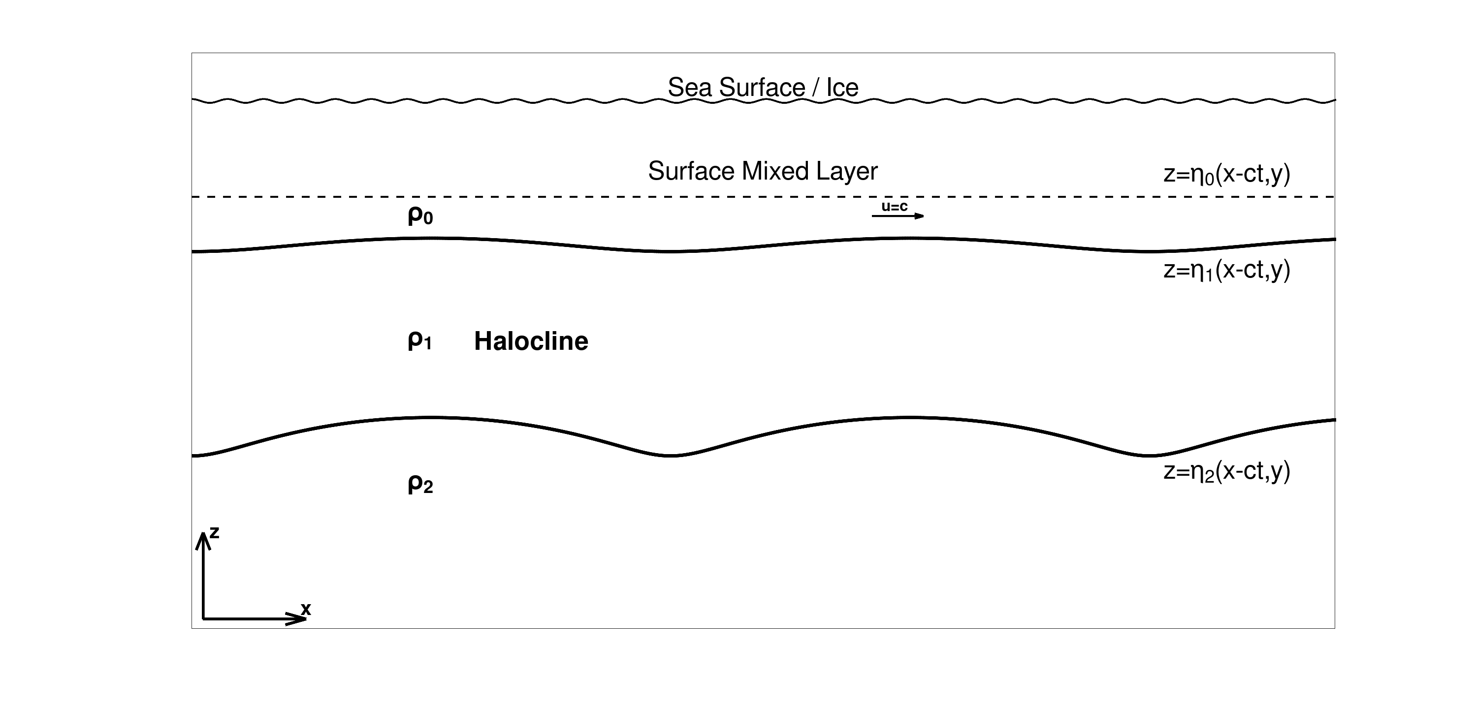
Figure 3.1. Schematic depiction of the flow pattern, at a fixed coordinate $y$

3.3.3. The dispersion relation

The last two equations in (3.34) and (3.41) are independent of $q,r,s$, therefore we can use them to write

$$\frac{\rho_{2}}{\rho_{1}}ga-ga-df\mathsf{c}=\left(\frac{\rho_{0}-\rho_{1}}{\rho_{1}}\right)(ga+f\mathsf{c}d)\Longrightarrow f\mathsf{c}d=\left(\frac{\rho_{2}-\rho_{0}}{\rho_{0}}\right)ga.$$ (3.45)

Defining the reduced gravity

$$\mathfrak{g}=\left(\frac{\rho_{2}-\rho_{0}}{\rho_{0}}\right)g,$$ (3.46)

we get

$$\mathsf{c}=\mathfrak{g}\frac{a}{fd},$$ (3.47)

that, making use of (3.29) and (3.30), gives the dispersion relation

$$f^{4}\mathsf{c}^{2}=\mathfrak{g}^{2}k^{2}\mathsf{c}^{2}-f^{2}\mathfrak{g}^{2},$$ (3.48)

which is equivalent to

$$\mathsf{c}^{2}=\frac{f^{2}\mathfrak{g}^{2}}{\mathfrak{g}^{2}k^{2}-f^{4}},$$ (3.49)

or

$$k^{2}=\frac{f^{4}}{\mathfrak{g}^{2}}+\frac{f^{2}}{\mathsf{c}^{2}}.$$ (3.50)

Observe that, (3.49) makes sense if and only if

$$\mathfrak{g}^{2}k^{2}-f^{4}>0\Longleftrightarrow k^{2}>\frac{f^{4}}{\mathfrak{g}^{2}},$$ (3.51)

as only $\mathsf{c}\in\mathbb{R}$ is valid in the context of Pollard (and Gerstner) waves, which is obviously satisfied due to (3.50). As $f^{4}\approx 10^{-16}$, from (3.49) it follows that

$$\mathsf{c}^{2}\approx\frac{f^{2}}{k^{2}},$$ (3.52)

therefore, the modulus of the period of the wave $T=\frac{L}{\mathsf{c}}$ is approximately $\frac{2\pi}{f}=T_{i}$, where $T_{i}$ is the inertial period of the Earth, so the wave motion describing the halocline surfaces is essentially inertial.
To provide a qualitative value of $k$ and consequently of the wavelength $L=\frac{2\pi}{k}$, we fix the reference parameters $\mathsf{c}\approx 0.1\,\mathrm{ms^{-1}}$, $\mathfrak{g}\approx 0.006\,\mathrm{ms^{-2}}$, $f=2\Omega\approx 1.5\cdot 10^{-4}\,\mathrm{s^{-1}}$. The dispersion relation (3.50) gives an approximate value of the wave number $k\approx 1.5\cdot 10^{-3}\,\mathrm{m^{-1}}$ the wavelength $L\approx 4.2\,\,\mathrm{km}$.

4. Other properties of the flow in the halocline layer

4.1. Vorticity

In contrast to the other layers, where the flow is irrotational, in the halocline the vorticity vector

$$\omega=\left(\frac{\partial w}{\partial y}-\frac{\partial v}{\partial z},\frac{\partial u}{\partial z}-\frac{\partial w}{\partial x},\frac{\partial v}{\partial x}-\frac{\partial u}{\partial y}\right)$$ (4.1)

is given by

$$\omega^{T}=\frac{1}{1-m^{2}a^{2}e^{-2ms}}\begin{pmatrix}\frac{m^{2}af}{k}e^{-ms}\sin\tau\\ \mathsf{c}a(k^{2}-m^{2})e^{-ms}\cos\tau+\mathsf{c}ma^{2}(m^{2}+k^{2})e^{-2ms}\\ fma(\cos\tau+mae^{-ms})e^{-ms}\end{pmatrix},$$ (4.2)

due to the relations

$$\left(\frac{\partial(q,r,s)}{\partial(x,y,z)}\right)\left(\frac{\partial(u,v,w)}{\partial(q,r,s)}\right)=\left(\frac{\partial(u,v,w)}{\partial(x,y,z)}\right),$$ (4.3)

$$\left(\frac{\partial(q,r,s)}{\partial(x,y,z)}\right)=\left(\frac{\partial(x,y,z)}{\partial(q,r,s)}\right)^{-1},$$

with

$$\left(\frac{\partial(q,r,s)}{\partial(x,y,z)}\right) =\begin{pmatrix}\frac{\partial q}{\partial x}&\frac{\partial r}{\partial x}&\frac{\partial s}{\partial x}\\ \frac{\partial q}{\partial y}&\frac{\partial r}{\partial y}&\frac{\partial s}{\partial y}\\ \frac{\partial q}{\partial z}&\frac{\partial r}{\partial z}&\frac{\partial s}{\partial z}\end{pmatrix}=$$ (4.4)

$$=\begin{pmatrix}\frac{1+kbe^{-ms}\cos\tau}{J}&-\frac{kde^{-ms}\sin\tau}{J}&-\frac{kae^{-ms}\sin\tau}{J}\\ 0&1&0\\ -\frac{mbe^{-ms}\sin\tau}{J}&-\frac{mde^{-ms}\cos\tau-m^{2}ad\,e^{-2ms}}{J}&\frac{1-mae^{-ms}\cos\tau}{J}\end{pmatrix},$$

where $J=1-m^{2}a^{2}e^{-2ms}$ is the determinant given in (3.15).
It is therefore evident that the flow is fully three-dimensional.
Observe that the velocity field $\boldsymbol{u}$ described in (3.19) does not depend on the variable $r$, therefore, as

$$\frac{\partial\boldsymbol{u}}{\partial y}=\frac{\partial\boldsymbol{u}}{\partial q}\frac{\partial q}{\partial y}+\frac{\partial\boldsymbol{u}}{\partial r}\frac{\partial r}{\partial y}+\frac{\partial\boldsymbol{u}}{\partial s}\frac{\partial s}{\partial y},$$ (4.5)

making use of (4.4), it follows that $\boldsymbol{u}$ does non depend on the coordinate $y$, namely

$$\frac{\partial u}{\partial y}=\frac{\partial v}{\partial y}=\frac{\partial w}{\partial y}=0.$$ (4.6)

Moreover,

$$\frac{\partial P}{\partial y}=\frac{\partial P}{\partial q}\frac{\partial q}{\partial y}+\frac{\partial P}{\partial r}\frac{\partial r}{\partial y}+\frac{\partial P}{\partial s}\frac{\partial s}{\partial y}=\frac{\partial P}{\partial r}=0,$$ (4.7)

where the last equality is due to (3.26), therefore also the pressure in independent of $y$ in the halocline layer.

4.2. Mean flow properties in the halocline layer

Following [20], we examine the mean velocities, the Stokes drift, and the mass flux for the internal water waves in the halocline layer. The mean Eulerian velocity is the mean velocity of the fluid at a fixed point, while the mean Lagrangian velocity is the mean velocity following a selected fluid particle. The Stokes drift $\mathbf{U}^{S}$ is the difference between the mean Lagrangian $\langle\boldsymbol{u}\rangle_{L}$ and the mean Eulerian velocity $\langle\boldsymbol{u}\rangle_{E}$,

$$\mathrm{U}^{S}=\langle\boldsymbol{u}\rangle_{L}-\langle\boldsymbol{u}\rangle_{E},$$ (4.8)

and finally we recall that, as noted by Stokes (see [36]), the mass transport is function of the mean Lagrangian velocity rather than the mean Eulerian one.
From the expression of the velocities in (3.19), we can calculate the mean Lagrangian velocities by averaging over a period $T=\frac{L}{\mathsf{c}}$, obtaining

$$\langle u\rangle_{L}=\frac{1}{T}\int_{0}^{T}k\mathsf{c}b\,e^{-ms}\cos\tau\,dt=0,$$ (4.9)

$$\langle v\rangle_{L}=-\frac{1}{T}\int_{0}^{T}k\mathsf{c}d\,e^{-ms}\sin\tau\,dt=0,$$

$$\langle w\rangle_{L}=-\frac{1}{T}\int_{0}^{T}k\mathsf{c}a\,e^{-ms}\sin\tau\,dt=0.$$

In order to obtain the mean Eulerian velocity, we need to compute the average of the wave velocity over the period at any fixed depth. As a fixed depth $z_{0}$ can be written, due to (3.7), as

$$z_{0}=-d_{0}+s-ae^{-ms}\cos\tau,$$ (4.10)

we can write the functional dependence $s=S(z_{0},\tau)$, where $W$ is the Lambert $W$-function, and $S=z_{0}-W(am\cos\tau e^{mz_{0}})$ (see [22]). Taking the derivative with respect to $q$ of (4.10) with $s=S(z_{0},\tau)$, we get

$$\frac{\partial S}{\partial q}=-\frac{kae^{-ms}\sin\tau}{1+mae^{-ms}\cos\tau}.$$ (4.11)

In order to obtain the mean Eulerian $u$-velocity, we write, adding and subtracting $\mathsf{c}$:

$$\langle u\rangle_{E}(z_{0}) =\frac{1}{T}\int_{0}^{T}\mathsf{c}+u(x-\mathsf{c}t,y,z_{0})\,dt-\mathsf{c}=\frac{1}{L}\int_{0}^{L}\mathsf{c}+u(x-\mathsf{c}t,y,z_{0})\,dx-\mathsf{c}$$ (4.12)

$$=\frac{1}{L}\int_{0}^{L}\left[\mathsf{c}+u(q-\mathsf{c}t,r,S(z_{0},\tau))\right]\frac{\partial x}{\partial q}\,dq-\mathsf{c}=$$

$$=\frac{1}{L}\int_{0}^{L}\mathsf{c}(1+ma\,e^{-mS}\cos\tau)\frac{1-m^{2}a^{2}\,e^{-2mS}}{1+mae^{-mS}\cos\tau}\,dq-\mathsf{c}=$$

$$=\mathsf{c}-\frac{m^{2}a^{2}\mathsf{c}}{L}\int_{0}^{L}e^{-2mS}\,dq-\mathsf{c}=-\frac{m^{2}a^{2}\mathsf{c}}{L}\int_{0}^{L}e^{-2mS}\,dq,$$

so the mean Eulerian $u$-velocity is opposite to the direction of propagation of the Pollard waves (parallel to the Transpolar Drift Current), whereas the other two Eulerian velocities are obtained by direct computations:

$$\langle v\rangle_{E}(z_{0}) =\frac{1}{T}\int_{0}^{T}v(x-\mathsf{c}t,y,z_{0})\,dt=\frac{1}{L}\int_{0}^{L}v(x-\mathsf{c}t,y,z_{0})\,dx$$ (4.13)

$$=\frac{1}{L}\int_{0}^{L}v(q-\mathsf{c}t,r,S(z_{0},\tau))\frac{\partial x}{\partial q}\,dq=$$

$$=\frac{1}{L}\int_{0}^{L}(-k\mathsf{c}d\,e^{-mS}\sin\tau)\frac{1-m^{2}a^{2}\,e^{-2mS}}{1+mae^{-mS}\cos\tau}\,dq=$$

$$=\frac{fma}{kL}\int_{0}^{L}(e^{-mS}\sin\tau)\frac{1-m^{2}a^{2}\,e^{-2mS}}{1+mae^{-mS}\cos\tau}\,dq,$$

$$\langle w\rangle_{E}(z_{0}) =\frac{1}{T}\int_{0}^{T}w(x-\mathsf{c}t,y,z_{0})\,dt=\frac{1}{L}\int_{0}^{L}w(x-\mathsf{c}t,y,z_{0})\,dx$$ (4.14)

$$=\frac{1}{L}\int_{0}^{L}w(q-\mathsf{c}t,r,S(z_{0},\tau))\frac{\partial x}{\partial q}\,dq=$$

$$=\frac{1}{L}\int_{0}^{L}(-k\mathsf{c}a\,e^{-mS}\sin\tau)\frac{1-m^{2}a^{2}\,e^{-2mS}}{1+mae^{-mS}\cos\tau}\,dq=$$

$$=-\frac{k\mathsf{c}a}{L}\int_{0}^{L}(e^{-mS}\sin\tau)\frac{1-m^{2}a^{2}\,e^{-2mS}}{1+mae^{-mS}\cos\tau}\,dq$$

where we have used (3.7), (3.14), (3.29) and the fact that

$$\frac{\partial x}{\partial q}=1+bm\frac{\partial S}{\partial q}e^{-mS}\sin\tau-kb\,e^{-mS}\cos\tau=\frac{1-m^{2}a^{2}\,e^{-2mS}}{1+mae^{-mS}\cos\tau},$$ (4.15)

whit the last equality coming from (4.11). The components of the Stokes drift, defined in (4.8), are therefore given by

$$U^{S} =\frac{m^{2}a^{2}\mathsf{c}}{L}\int_{0}^{L}e^{-2mS}\,dq,$$ (4.16)

$$V^{S} =-\frac{fma}{kL}\int_{0}^{L}(e^{-mS}\sin\tau)\frac{1-m^{2}a^{2}\,e^{-2mS}}{1+mae^{-mS}\cos\tau}\,dq,$$

$$W^{S} =\frac{k\mathsf{c}a}{L}\int_{0}^{L}(e^{-mS}\sin\tau)\frac{1-m^{2}a^{2}\,e^{-2mS}}{1+mae^{-mS}\cos\tau}\,dq\,.$$

Finally, we compute the mass fluxes. As the motion of the water particles in the halocline in three-dimensional, we consider the flux through three orthogonal planes.
The mass flux through a plane $\Sigma$ is defined as

$$\mathcal{M}=\int_{\Sigma}\rho\boldsymbol{u}\cdot\boldsymbol{\mathfrak{n}}\,d\Sigma,$$ (4.17)

where $\boldsymbol{\mathfrak{n}}$ in the normal vector to the surface $\Sigma$. As we are considering the halocline layer, we set constant density $\rho=\rho_{1}$.
We begin with the mass flux in the $x$-direction. Let us fix at $x=x_{0}$ the plane $\Sigma^{x}=\left[\eta_{2},\eta_{1}\right]\times\left[y_{1},y_{2}\right]$, with $y_{1}<y_{2}$. The mass flux in the $x$-direction is given by

$$\mathcal{M}^{x} =\rho_{1}\iint_{\left[\eta_{2},\eta_{1}\right]\times\left[y_{1},y_{2}\right]}u(x_{0}-ct,y,z)\,dz\,dy$$ (4.18)

$$=\rho_{1}\int_{\mathrm{s_{-}}}^{\mathrm{s_{+}}}\int_{-\mathrm{r_{0}}}^{\mathrm{r_{0}}}u\det\begin{pmatrix}\partial_{r}y&\partial_{s}y\\ \partial_{r}z&\partial_{s}z\end{pmatrix}dr\,ds.$$

Having fixed $x=x_{0}$ implies a functional relation

$$q=\beta(x_{0},s,t).$$ (4.19)

Taking the $s$-derivative of

$$x_{0}=q-be^{-ms}\sin\tau=\beta(x_{0},s,t)-be^{-ms}\sin\tau,$$ (4.20)

gives

$$\frac{\partial\beta}{\partial s}=-\frac{bme^{-ms}\sin\tau}{1-ma^{-ms}\cos\tau}.$$ (4.21)

From (3.11), we have

$$\frac{\partial y}{\partial r}=1,\quad\frac{\partial z}{\partial r}=0,$$ (4.22)

and, due to the relations

$$\left.\begin{aligned} z=-d_{0}+s-ae^{-ms}\cos\tau\\ q=\beta(x_{0},s,t)\\ \frac{\partial\beta}{\partial s}=-\frac{bme^{-ms}\sin\tau}{1-ma^{-ms}\cos\tau}\end{aligned}\right\}\Longrightarrow\frac{\partial z}{\partial s}=\frac{1-m^{2}a^{2}e^{-2ms}}{1-mae^{-ms}\cos\tau}.$$ (4.23)

Therefore, from (4.18), the mass flux in the $x$-direction is

$$\mathcal{M}^{x}=\rho_{1}\mathsf{c}ma\int_{\mathrm{s_{-}}}^{\mathrm{s_{+}}}e^{-ms}\cos\tau\frac{1-m^{2}a^{2}e^{-2ms}}{1-mae^{-ms}\cos\tau}\,ds.$$ (4.24)

As $\langle u\rangle_{L}=0$, we expect that the mass flux (4.23) is zero, when averaged over a wave period $T$. This assertion is in fact true: by differentiating with respect to $t$ (4.20) one gets

$$\frac{\partial\beta}{\partial t}=-\frac{\mathsf{c}mae^{-ms}\cos\tau}{1-ma^{-ms}\cos\tau}$$ (4.25)

for the $T$-periodic function $t\mapsto\beta(x_{0},s,t)$, hence (4.24) reads as

$$\mathcal{M}^{x}=\rho_{1}\int_{\mathrm{s_{-}}}^{\mathrm{s_{+}}}\left(m^{2}a^{2}e^{-2ms}-1\right)\frac{\partial\beta}{\partial t}\,ds,$$ (4.26)

implying

$$\int_{0}^{T}\mathcal{M}^{x}\,dt=0.$$ (4.27)

Let us now compute the mass flux in the $y$-direction by fixing at $y=y_{0}$ the plane $\Sigma^{y}=\left[\eta_{2},\eta_{1}\right]\times\left[0,L\right]$, where $L=\frac{2\pi}{k}$ is the wave length. The mass flux in the $y$-direction is given by

$$\mathcal{M}^{y} =\rho_{1}\iint_{\left[\eta_{2},\eta_{1}\right]\times\left[0,L\right]}v(x-ct,y_{0},z)\,dz\,dx$$ (4.28)

$$=\rho_{1}\int_{\mathrm{s_{-}}}^{\mathrm{s_{+}}}\int_{0}^{L}v\det\begin{pmatrix}\partial_{q}x&\partial_{s}x\\ \partial_{q}z&\partial_{s}z\end{pmatrix}dq\,ds.$$

As the variables $x$ and $z$ are independent of $r$ (see (3.7) and (3.11)), there is no need to write a functional relation for fixed $y=y_{0}$. Consequently, the mass flux in the $y$-direction is

$$\mathcal{M}^{y}=\rho_{1}\frac{fma}{k}\int_{\mathrm{s_{-}}}^{\mathrm{s_{+}}}\int_{0}^{L}e^{-ms}\sin\tau\left(1-m^{2}a^{2}e^{-2ms}\right)\,dqds,$$ (4.29)

where me also used the relation (3.29). It is immediate to see that

$$\int_{0}^{T}\mathcal{M}^{y}\,dt=0,$$ (4.30)

as expected, since $\langle v\rangle_{L}=0$.
Finally, for the mass flux in the $z$-direction, let us fix at $z=z_{0}$ the plane $\Sigma^{z}=[0,L]\times[y_{1},y_{2}]$, where $z_{0}$ is chosen between the crest $\mathrm{z}_{-}$ of the halocline lower surface $\eta_{2}$ and the trough $\mathrm{z}_{+}$ of the halocline upper surface $\eta_{1}$, that is $\mathrm{z}_{-}<z_{0}<\mathrm{z}_{+}$. We write the functional relation

$$s=\xi(z_{0},q,t).$$ (4.31)

Writing, according to (3.7)

$$z_{0}=s-ae^{-ms}\cos\tau,$$ (4.32)

we get

$$\frac{\partial\xi}{\partial q} =-\frac{kae^{-m\xi}\sin\tau}{1+mae^{-m\xi}\cos\tau},$$ (4.33)

$$\frac{\partial\xi}{\partial t} =\frac{k\mathsf{c}ae^{-m\xi}\sin\tau}{1+mae^{-m\xi}\cos\tau}.$$ (4.34)

Equation (4.33) gives

$$\frac{\partial x}{\partial q}=\frac{1-m^{2}a^{2}e^{-2m\xi}}{1+mae^{-m\xi}\cos\tau},$$ (4.35)

and, since from (3.11) we have

$$\frac{\partial x}{\partial r}=0,\quad\frac{\partial y}{\partial r}=1,$$ (4.36)

the mass flux in the $z$-direction, defined as

$$\mathcal{M}^{z} =\rho_{1}\iint_{\left[0,L\right]\times[y_{1},y_{2}]}w(x-ct,y,z_{0})\,dz\,dx$$ (4.37)

$$=\rho_{1}\int_{0}^{L}\int_{-\mathrm{r_{0}}}^{\mathrm{r_{0}}}w\det\begin{pmatrix}\partial_{q}x&\partial_{r}x\\ \partial_{q}y&\partial_{r}y\end{pmatrix}dq\,dr,$$

is given by

$$\mathcal{M}^{z}=-2\rho_{1}\mathrm{r_{0}}\int_{0}^{L}k\mathsf{c}ae^{-m\xi}\sin\tau\frac{1-m^{2}a^{2}e^{-2m\xi}}{1+mae^{-m\xi}\cos\tau}\,dq.$$ (4.38)

Furthermore, as

$$\mathcal{M}^{z}=-2\rho_{1}\mathrm{r_{0}}\int_{0}^{L}\left(1-m^{2}a^{2}e^{-2m\xi}\right)\frac{\partial\xi}{\partial t}\,dq,$$ (4.39)

due to (4.34), and the function $t\mapsto\xi(z_{0},q,t)$ being $T$-periodic, we get

$$\int_{0}^{T}\mathcal{M}^{z}\,dt=0,$$ (4.40)

as could be inferred by $\langle w\rangle_{L}=0.$
In conlusion, this prove that the Pollard internal wave has no net wave transport over a wave period.

5. Comparison with the linearized Lagrangian version of the problem

Linearizing about the hydrostatic solution $x=q,\ y=r,\ z=s$ the governing equations in Lagrangian form (see [22] and [30]), namely

$$\left\{\begin{aligned} &\left(\frac{\partial^{2}x}{\partial t^{2}}-f\frac{\partial y}{\partial t}\right)\frac{\partial x}{\partial q}+\left(\frac{\partial^{2}y}{\partial t^{2}}+f\frac{\partial x}{\partial t}\right)\frac{\partial y}{\partial q}+\frac{\partial^{2}z}{\partial t^{2}}\frac{\partial x}{\partial q}+g\frac{\partial z}{\partial q}=-\frac{1}{\rho}\frac{\partial P}{\partial q},\\ &\left(\frac{\partial^{2}x}{\partial t^{2}}-f\frac{\partial y}{\partial t}\right)\frac{\partial x}{\partial r}+\left(\frac{\partial^{2}y}{\partial t^{2}}+f\frac{\partial x}{\partial t}\right)\frac{\partial y}{\partial r}+\frac{\partial^{2}z}{\partial t^{2}}\frac{\partial x}{\partial r}+g\frac{\partial z}{\partial r}=-\frac{1}{\rho}\frac{\partial P}{\partial r},\\ &\left(\frac{\partial^{2}x}{\partial t^{2}}-f\frac{\partial y}{\partial t}\right)\frac{\partial x}{\partial s}+\left(\frac{\partial^{2}y}{\partial t^{2}}+f\frac{\partial x}{\partial t}\right)\frac{\partial y}{\partial s}+\frac{\partial^{2}z}{\partial t^{2}}\frac{\partial x}{\partial s}+g\frac{\partial z}{\partial q}=-\frac{1}{\rho}\frac{\partial P}{\partial s},\end{aligned}\right.$$ (5.1)

and

$$\frac{d}{dt}\left(\det\left(\frac{\partial(x,y,z)}{\partial(q,r,s)}\right)\right)=0,$$ (5.2)

which are the Euler equations and the incopressibility condition, respectively, yield to the linearized Euler equations

$$\left\{\begin{aligned} &\frac{\partial^{2}x}{\partial t^{2}}-f\frac{\partial y}{\partial t}+g\frac{\partial z}{\partial q}=-\frac{1}{\rho_{1}}\frac{\partial P}{\partial q},\\ &\frac{\partial^{2}y}{\partial t^{2}}+f\frac{\partial x}{\partial t}+g\frac{\partial z}{\partial r}=-\frac{1}{\rho_{1}}\frac{\partial P}{\partial r},\\ &\frac{\partial^{2}z}{\partial t^{2}}+g\frac{\partial z}{\partial s}=-\frac{1}{\rho_{1}}\frac{\partial P}{\partial s},\end{aligned}\right.$$ (5.3)

and the linearized incompressibility condition

$$\frac{\partial^{2}x}{\partial q\partial t}+\frac{\partial^{2}y}{\partial r\partial t}+\frac{\partial^{2}z}{\partial s\partial t}=0.$$ (5.4)

Remarkably, Pollard waves (3.7) are solutions also to the system of linearized equations (5.3) and (5.4). Namely, writing

$$\left\{\begin{aligned} &x=q-be^{-ms}\sin(k(q-\mathsf{c}t)),\\ &y=r-de^{-ms}\cos(k(q-\mathsf{c}t)),\\ &z=-d_{0}+s-ae^{-ms}\cos(k(q-\mathsf{c}t)),\end{aligned}\right.$$ (5.5)

the incompressiblity equation (5.4) is reduced to the condition (3.14):

$$b=\frac{am}{k}.$$ (5.6)

Rewriting (5.3) as

$$\left\{\begin{aligned} &\frac{\partial P}{\partial q}=-\rho_{1}\left[\frac{\partial^{2}x}{\partial t^{2}}-f\frac{\partial y}{\partial t}+g\frac{\partial z}{\partial q}\right],\\ &\frac{\partial P}{\partial r}=-\rho_{1}\left[\frac{\partial^{2}y}{\partial t^{2}}+f\frac{\partial x}{\partial t}+g\frac{\partial z}{\partial r}\right],\\ &\frac{\partial P}{\partial s}=-\rho_{1}\left[\frac{\partial^{2}z}{\partial t^{2}}+g\frac{\partial z}{\partial s}\right],\end{aligned}\right.$$ (5.7)

gives, for the pressure, the solution

$$P=\widetilde{P_{1}}-\rho_{1}gs+\rho_{1}\left[\frac{k^{2}\mathsf{c}^{2}a}{m}+ga\right]e^{-ms}\cos\tau,$$ (5.8)

with the conditions

$$k\mathsf{c}d+fb=0,$$ (5.9)

$$m^{2}=\frac{k^{4}\mathsf{c}^{2}}{\mathsf{c}^{2}k^{2}-f^{2}},$$ (5.10)

and where, again,

$$\tau=k(x-\mathsf{c}t).$$ (5.11)

We remark that the conditions (5.6), (5.9) and (5.10) are exactly those found in the nonlinear analysis: (3.14), (3.24) and (3.25).
Recalling the the dynamic boundary condition (namely the continuity of the pressure across the halocline top and bottom surfaces):

$$P=\begin{cases}P_{0}-\rho_{0}gz-\rho_{0}f\mathsf{c}y\quad\text{for}\ z=\eta_{1},\\ P_{2}-\rho_{2}gz\quad\qquad\text{for}\ z=\eta_{2},\end{cases}$$ (5.12)

we see that this is equivalent to

$$\left\{\begin{aligned} &P_{0}-\widetilde{P_{1}}=-(\rho_{1}-\rho_{0})g\mathrm{s}_{+}+\rho_{0}f\mathsf{c}r-\rho_{0}gd_{0},\\ &bk\mathsf{c}^{2}=\left(\frac{\rho_{0}-\rho_{1}}{\rho_{1}}\right)(ga+f\mathsf{c}d),\end{aligned}\right.$$ (5.13)

where $s=\mathrm{s}_{+}$ represent the upper surface of the halocline $\eta_{1}$, while on the lower surface $\eta_{2}$ represented by $s=\mathrm{s}_{-}$, it is given by

$$\left\{\begin{aligned} &P_{2}-\widetilde{P_{1}}=(\rho_{2}-\rho_{1})g\mathrm{s}_{-}-\rho_{2}gd_{0},\\ &bk\mathsf{c}^{2}=\frac{\rho_{2}}{\rho_{1}}ga-ga-df\mathsf{c},\end{aligned}\right.$$ (5.14)

therefore we recover again the dispersion relation (3.49):

$$\mathsf{c}^{2}=\frac{f^{2}\mathfrak{g}^{2}}{\mathfrak{g}^{2}k^{2}-f^{4}},$$ (5.15)

and we note that the pressure (3.32) of Pollard’s exact solution represent a higher order correction of the one related to the linear case just examined (5.8).

6. Discussion

We conclude by presenting some qualitative and quantitative considerations for the solution (3.7).
Let us recall (3.49) and (3.50):

$$\mathsf{c}^{2}=\frac{f^{2}\mathfrak{g}^{2}}{\mathfrak{g}^{2}k^{2}-f^{4}},\qquad k^{2}=\frac{f^{4}}{\mathfrak{g}^{2}}+\frac{f^{2}}{\mathsf{c}^{2}},$$ (6.1)

where $\mathfrak{g}=\left(\frac{\rho_{2}-\rho_{0}}{\rho_{0}}\right)g$. As a consequence, the dispersion relation depends, in addition to $f$, only on $\rho_{2}$ and $\rho_{0}$, namely on the density of the water above and below the halocline, and not on the density of its water $\rho_{1}$. However, this dependence is very marginal. Observe also that the the wavelength increases (very slightly) as $\mathfrak{g}$ increases (i.e. when the density difference between the warmer and saltier Atlantic Water and the fresher and colder water of the Surface Mixing Layer increases). Fixing the parameters describing the flow under consideration, $\mathsf{c}\approx 0.1\,\mathrm{ms^{-1}}$, $\mathfrak{g}\approx 0.006\,\mathrm{ms^{-2}}$, $f=2\Omega\approx 1.5\cdot 10^{-4}\,\mathrm{s^{-1}}$, due to relations (3.30) and (3.50), we can obtain an approximate value for

$$m^{2}=\frac{f^{4}}{\mathfrak{g}^{2}}+\frac{\mathfrak{g}^{2}}{\mathsf{c}^{4}}+2\frac{f^{2}}{\mathsf{c}^{2}}\approx\frac{\mathfrak{g}^{2}}{\mathsf{c}^{4}}=0.36\,\mathrm{m^{-2}},$$ (6.2)

giving

$$m\approx 0.6\,\mathrm{m^{-2}},$$ (6.3)

and $k\approx 1.5\cdot 10^{-3}\,\mathrm{m^{-1}}$, as already seen in Section 3. From (3.7) it is immediate to see that as depth increases, the amplitude of the waves increases and the maximum oscillation of the wave will be less than $\frac{10}{6}\approx 1.67\,\mathrm{m}$, in view of (3.17), and, due to the relation (6.2), a variation in $\mathfrak{g}$ will influence the wave amplitude more than the wave length.
Moreover, as the amplitude of the waves described in (3.7) increases when the depth of the halocline reduces, we can infer that in summer - with the decreasing of the depths of the halocline boundaries [29] - the amplitude of the oscillations will decrease, and vice-versa in winter. That said, due to the exponential factor $e^{-ms}$ of (3.7), such increment/decrement of the amplitude in different seasons would hardly be detectable.
About the halocline’s upper surface, as anticipated, (3.39) shows that the upper surface of the halocline reduces its depth as $r$ increases (namely in the Eurasian Basin), and increases in depth as $r$ decreases (namely in the Amerasian Basin). This result matches the measurements made by oceanographers (see [32]), even if we infer that there should be other, physical processes influencing the halocline depth, such as water inflows from other basins, against these variations. In fact, from (3.39) we have that

$$\mathrm{s}^{\prime}_{+}(r)=\frac{\rho_{0}f\mathsf{c}}{2mAe^{-2m\mathrm{s}_{+}(r)}+(\rho_{1}-\rho_{0})g}<\left(\frac{(\rho_{1}-\rho_{0})g}{\rho_{0}}\right)^{-1}f\mathsf{c}\lesssim 0.019,$$ (6.4)

thus, an increase [decrease] in $r$ of kilometers produces an decrease [increase] in the depth of the halocline’s upper surface of tens of meters. As depth variations of the halocline are less than a hundred meters in different basins (see [32] or [34]), we deduce that such variations must be controlled also by other physical processes.
Recalling that the particle motion in (3.7) describes trochoidal orbits, namely the path of a fixed point on a circle of radius $be^{-ms}$ and centered at $(q,r,s-d_{0})$, rolling along the $x$-axis, in a plane that is at an angle $\arctan\left(-\frac{d}{a}\right)$ with respect to the vertical axis, due to (3.29), we have that

$$\arctan\left(-\frac{d}{a}\right)=\arctan\left(\frac{m}{\frac{f^{3}\mathsf{c}}{\mathfrak{g}^{2}}+\frac{f}{\mathsf{c}}}\right)\lesssim\frac{\pi}{2},$$ (6.5)

and, using (3.17),

$$|d|<\frac{f}{k^{2}\mathsf{c}}\approx 667\,\mathrm{m}.$$ (6.6)

Namely, the throcoidal orbit described in (3.7) is almost horizontal with oscillations not exceeding $667\,\mathrm{m}$, describing small-amplitude, near-inertial, Pollard waves moving parallel to the Transpolar Drift Current.
As pointed out by Garret & Munk (see [14] and [15]), near-inertial waves are the most energetic ones, but are hard to detect, even without the presence of ice (e.g. using satellite methods [40]).
We point out the simple near-inertial dispersion relation obtained in (3.49), imposed by the two dynamic boundary conditions at the halocline surfaces, in contrast to other works - with only one dynamic boundary condition - having much more complicated dispersion relations, describing two wave modes (one slow, near inertial and one faster) whose formulae were obtained via a perturbative analysis of the dispersion relation, and not in closed form [12], [25], [26].

Funding

The author is supported by the Austrian Science Fund (FWF) [grant number Z 387-N].

References

- [1] A. A. Abrashkin, E. N. Pelinovsky, Gerstner waves and their generalizations in hydrodynamics and geophysics, Phys. Usp., Vol. 65 (2022), 453–467.
- [2] C. Bertosio, On the evolution of the halocline in the upper Arctic Ocean since 2007, PhD Thesis in Oceanography, Sorbonne Université, 2021.
- [3] E. C. Carmack, The alpha/beta ocean distinction: A perspective on freshwater fluxes, convection, nutrients and productivity in high-latitude seas, Deep-Sea Res. II, Vol. 54 (2007), 2578–2598.
- [4] W. Chinn, and N. Steenrod “First Concepts of Topology”, Mathematical Association of America, Washington DC, 1966.
- [5] A. Constantin, “Nonlinear water waves with applications to wave-current interactions and tsunamis”, Society for Industrial and Applied Mathematics, Philadelphia, 2011.
- [6] A. Constantin, An exact solution for equatorially trapped waves, J. Geophys. Res., Vol. 117 (2012), C05029.
- [7] A. Constantin, Some Three-Dimensional Nonlinear Equatorial Flows, J. Phys. Oceanogr., Vol. 43 (2013), 165–175.
- [8] A. Constantin, Some Nonlinear, Equatorially Trapped, Nonhydrostatic Internal Geophysical Waves, J. Phys. Oceanogr., Vol. 44 (2014), 781–789.
- [9] A. Constantin, and R. S. Johnson, On the role of nonlinearity in geostrophic ocean flows on a sphere, In: N. Euler (Ed.), Nonlinear Systems and Their Remarkable Mathematical Structures: Volume I, CRC Press Taylor & Francis Group, Boca Raton, 2019.
- [10] A. Constantin, and R. S. Johnson, On the dynamics of the near-surface currents in the Arctic Ocean, Nonlinear Anal., Real World Appl., Vol. 73 (2023), 103894.
- [11] A. Constantin, and R. S. Johnson, Spherical Coordinates for Arctic Ocean Flows, In: D. Henry (Ed.), Nonlinear Dispersive Waves. Advances in Mathematical Fluid Mechanics. Birkhäuser, Cham, 2024.
- [12] A. Constantin, and S. G. Monismith, Gerstner waves in the presence of mean currents and rotation, J. Fluid Mech., Vol. 820 (2017), 511-528.
- [13] A. Constantin, and P. Germain, Instability of some equatorially trapped waves, J. Geophys. Res. Oceans, Vol. 118 (2013), 2802–2810.
- [14] C. J. Garrett, and W. H. Munk, Space-time scales of internal waves, Geophys. Fluid Dyn., Vol. 2 (1972), 225–264.
- [15] C. J. Garrett, and W. H. Munk, Space-time scales of internal waves: A progress report, J. Geophys. Res., Vol. 80 (1975), 291–297.
- [16] F. Gerstner, Theorie der Wellen, Ann. Phys., Vol. 32 (1809), 412-445.
- [17] A. E. Gill, “Atmosphere-Ocean Dynamics”, Academic Press, London, 1982.
- [18] J. D. Guthrie, J. H. Morison, and I. Fer, Revisiting internal waves and mixing in the Arctic Ocean, J. Geophys. Res. Oceans, Vol. 118 (2013), 3966–3977.
- [19] D. Henry, On Gerstner’s Water Wave, J. Nonlinear Math. Phys., Vol. 15 (2008), 87-95.
- [20] M. Kluczek, Physical flow properties for Pollard-like internal water waves, J. Math. Phys. Vol. 59 (2018), 123102.
- [21] M. Kluczek, Nonhydrostatic Pollard-like internal geophysical waves, Discrete Continuous Dyn. Syst., Vol. 39 (2019), 5171-5183.
- [22] M. Kluczek, and R. Stuhlmeier, Mass transport for Pollar waves, Appl. Anal., Vol. 101 (2020), 984–993.
- [23] J. Marshall, and R. A. Plumb, “Atmosphere, Ocean and Climate Dynamics. An Introductory Text”, Academic Press, Burlington, 2008.
- [24] E. P. Metzner, and M. Salzmann, Technical note: Determining Arctic Ocean halocline and cold halostad depths based on vertical stability, Ocean Sci., Vol. 19 (2023), 1453–1464.
- [25] J. McCarney, Exact internal waves in the presence of mean currents and rotation, J. Math. Phys., Vol. 64 (2023), 073101.
- [26] J. McCarney, Nonhydrostatic internal waves in the presence of mean currents and rotation, J. Math. Phys., Vol. 65 (2024), 043101.
- [27] O. Morita, Classical Mechanics in Geophysical Fluid Dynamics, CRC Press, 2023.
- [28] A. J. G. Nurser, and S. Bacon, The Rossby radius in the Arctic Ocean, Ocean Sci., Vol. 10 (2014), 967–975.
- [29] C. Peralta-Ferriz, and R. A. Woodgate, Seasonal and interannual variability of pan-Arctic surface mixed layer properties from 1979 to 2012 from hydrographic data, and the dominance of stratification for multiyear mixed layer depth shoaling, Progress in Oceanography, Vol. 134 (2015), 19–53.
- [30] W. J. Pierson Jr., “Models of Random Seas Based on the Lagrangian Equations of Motion”, College of Eng., Res. Div., New York University, New York, 1961.
- [31] R. T. Pollard, Surface waves with rotation: an exact solution, J. Geophys. Res., Vol. 75 (1970), 5895-5898.
- [32] I. V. Polyakov, A. V. Pnyushkov, and E. C. Carmack, Stability of the arctic halocline: a new indicator of arctic climate change, Environ. Res. Lett., Vol. 13 (2018), 125008.
- [33] C. Puntini, On the modeling of nonlinear wind-induced ice-drift ocean currents at the North Pole, Preprint, https://arxiv.org/pdf/2503.12906.
- [34] B. Rudels, and E. Carmack, Arctic Ocean Water Mass Structure and Circulation, Oceanography, Vol. 35 (2022), 52-65.
- [35] R. Salmon, “Lectures on Geophysical Fluid Dynamics”, Oxford University Press, New York, 1998.
- [36] G. G. Stokes, On the Theory of Oscillatory Waves, Trans. Cambridge Philos. Soc., Vol. 8 (1847), 441-455.
- [37] L. D. Talley, G. L. Pickard, W. J. Emery, and J. H. Swift, “Descriptive Physical Oceanography: An Introduction”, Elsevier, Amsterdam, 2011.
- [38] M.-L. Timmermans, and J. Marshall, Understanding Arctic Oceancirculation: A review of oceandynamics in a changing climate, J. Geophys. Res. Oceans, Vol. 125 (2020), e2018JC014378.
- [39] G. K. Vallis, “Atmospheric and Oceanic Fluid Dynamics. Fundamentals and Large-Scale Circulation”, Cambridge University Press, Cambridge, 2017.
- [40] W. B. White, and R. G. Peterson, An Antarctic circumpolar wave in surface pressure, temperature and sea-ice extent, Nature, Vol. 380 (1996) , 699-702.