High-Performance Gradient Evaluation for Complex Soft Materials Using MPI-based DFS Algorithm

Abstract

This article presents a depth-first search (DFS)-based algorithm for evaluating sensitivity gradients in the topology optimization of soft materials exhibiting complex deformation behavior. The algorithm is formulated using a time-dependent adjoint sensitivity approach and is implemented within a PETSc-based C++ MPI framework for efficient parallel computing. It has been found that on a single processor, the sensitivity analysis for these complex materials can take approximately 45 minutes. This necessitates the use of high-performance computing (HPC) to achieve feasible optimization times. This work provides insights into the algorithmic framework and its application to large-scale generative design for physics integrated simulation of soft materials under complex loading conditions.

1 Introduction

Shape memory polymers (SMPs) are a class of active polymeric materials that have the ability to regain their original undeformed configuration from a deformed state under the application of an external stimulus. A time-dependent adjoint sensitivity formulation implemented through a recursive algorithm is used to calculate the gradients required for the topology optimization algorithm. For 3D SMPTO code, ran on UIUC campus-cluster, the time taken for single optimization iteration amounts to approximately 10 hours on 200 processors for a 3D mesh of 50$\times$ 20 $\times$ 20 elements with 60, 000 degrees-of-freedom. Our aim is to get the maximum number of optimization iterations completed within a specific unit of time, which would demand resources beyond the current allowable limit of the UIUC campus-cluster. The code is provided in the github repository[2]. This article provides a detailed explanation of the PETSc-based algorithm implemented in thesis[1] to provide interested readers with additional background information.

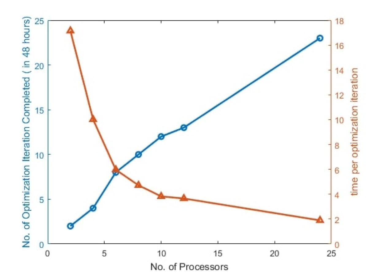
Figure 1: Scaling capability study performed using UIUC campus-cluster

2 Sensitivity Analysis

Time-dependent adjoint sensitivity analysis is performed to calculate the gradient information required for the structural optimization process. The procedure here describes the calculation of adjoint sensitivities. The function of interest being differentiated is the displacement at a particular degree-of-freedom ($a$) of the structure, at a particular time step ($M$) as shown in Figure (2).

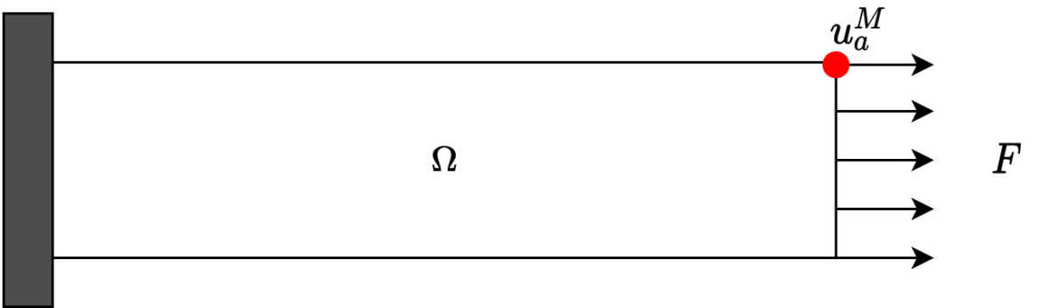
Figure 2: Design domain for sensitivity calculations and its verification.

Let the scalar function of interest($\theta$) be defined as

$$\theta={\bm{u}_{a}^{M}(\rho)}$$ (1)

Let $\bm{u^{M}(\rho)}$ represent the displacement vector of the whole structure at time step $M$. Then we can write Equation(1) as

$$\theta=\bm{L}^{T}\bm{u}^{M}(\rho)$$ (2)

where $\bm{L}$ is a column vector and is zero everywhere except at the entry corresponding to the $a^{th}$ degree-of-freedom. We can form an augmented Lagrangian function as

$$\Theta=\theta+\sum_{i=1}^{M}\Bigg{[}{\bm{\lambda}^{(i)}}^{T}\bm{R}^{(i)}(\bm{\rho},\bm{u}^{i},\bm{u}^{i-1},....,\bm{u}^{0})\Bigg{]}$$ (3)

where $\bm{\rho}$ is the design variable and the variable $\bm{u}$ is the state variable(containing all the variables evaluated through forward analysis). Note that $\Theta=\theta$ since $R^{(i)}=0$ for all i. Therefore $\frac{d\Theta}{d\mathbf{\rho}}=\frac{d\theta}{d\mathbf{\rho}}$. Differentiating Equation (3) with respect to the design variable $\bm{\rho}$, we obtain

$$\frac{d\Theta}{d\bm{\rho}} =L^{T}\frac{d\bm{u}^{M}}{d\bm{\rho}}+\sum_{i=1}^{M}\Bigg{[}{\bm{\lambda}^{(i)}}^{T}\Bigg{(}\sum_{k=1}^{i}\frac{\partial\bm{R}^{(i)}}{\partial\bm{\bm{u}}^{(k)}}\frac{d\bm{u}^{(k)}}{d\bm{\rho}}+\frac{\partial\bm{R}^{(i)}}{\partial\bm{\bm{\rho}}}\Bigg{)}\Bigg{]}$$ (4)

Expanding the right-hand side terms yields

$$\begin{split}\frac{d\Theta}{d\bm{\rho}}&=L^{T}\frac{d\bm{u}^{M}}{d\bm{\rho}}+\sum_{i=1}^{M}{\bm{\lambda}^{(i)}}^{T}\frac{\partial\bm{R}^{(i)}}{\partial\bm{\bm{\rho}}}+{\bm{\lambda}^{(M)}}^{T}\Bigg{(}\frac{\partial\bm{R}^{(M)}}{\partial\bm{u}^{(M)}}\frac{d\bm{u}^{(M)}}{d\bm{\rho}}\Bigg{)}+\sum_{i=1}^{M-1}\sum_{k=i}^{M}\Bigg{(}{\bm{\lambda}^{(k)}}^{T}\frac{\partial\bm{R}^{(k)}}{\partial\bm{\bm{u}}^{(i)}}\Bigg{)}\frac{d\bm{u}^{(i)}}{d\bm{\rho}}\\ \end{split}$$ (5)

The solution of {$\bm{\lambda}^{i}$} which causes all the implicit terms, $\{\frac{d\bm{u}}{d\bm{\rho}}\}$, to vanish is given by

$$\begin{split}\bm{\lambda}^{(M)}&=-L^{T}\Bigg{[}\frac{\partial\bm{R}^{(M)}}{\partial\bm{u}^{(M)}}\Bigg{]}^{-1}\\ \bm{\lambda}^{(i)}&=-\Bigg{[}\sum_{k=i+1}^{M}{\bm{\lambda}^{(k)}}^{T}\frac{\partial\bm{R}^{(k)}}{\partial\bm{u}^{(i)}}\Bigg{]}\Bigg{[}\frac{\partial\bm{R}^{(i)}}{\partial\bm{u}^{(i)}}\Bigg{]}^{-1}\\ \ \end{split}$$ (6)

When solved in this way the parameters {$\bm{\lambda}^{i}$} are referred to as the $\it{adjoint}$ vectors, and each vector $\bm{\lambda^{i}}$ represents the adjoint state at each time step $t_{i}$. Algorithm 1 contains a pseudocode description of the algorithm used to compute the sensitivities of the SMP material.

$\frac{df}{d\bm{\rho}}\leftarrow\frac{\partial}{d\bm{\rho}}\left[f(\bm{\rho},{\bm{u}}^{(M)})\right]$ // initialize sensitivities

$\bm{\lambda}^{(M)}\leftarrow{\left[\frac{\partial\bm{R}^{(M)}}{\bm{u}^{(M)}}\right]}^{-1}\left[-\frac{\partial f}{\bm{u}^{(M)}}\right]$ // solve for final adjoint state

for $i\leftarrow M,M-1,\dots,0$ do

   // cycle back through each time step

   ${\bm{F}_{RHS}}\leftarrow 0$

   // Cycle forward through all subsequent time steps

   for $k\leftarrow i+1,i+2,\dots,M$ do

     $\frac{\partial{\bm{R}}^{(k)}}{\partial{\bm{u}}^{(i)}}\leftarrow\frac{\partial{\bm{\varepsilon}}^{ir}_{(k)}}{\partial\bm{\varepsilon}^{r}_{(i)}}+\frac{\partial{\bm{\varepsilon}}^{ig}_{(k)}}{\partial\bm{\varepsilon}^{r}_{(i)}}+\frac{\partial{\bm{\varepsilon}}^{i}_{(k)}}{\partial\bm{\varepsilon}^{r}_{(i)}}+\frac{\partial{\bm{\varepsilon}}^{is}_{(k)}}{\partial\bm{\varepsilon}^{r}_{(i)}}$

     // Each additive term is traced back in time through the recursive Algorithm 2 and Algorithm 3

     ${\bm{F}_{RHS}}\leftarrow{\bm{F}_{RHS}}-\left[{\bm{\lambda}}^{(k)}\frac{\partial{\bm{R}}^{(k)}}{\partial{\bm{u}}^{(i)}}\right]$

    

     ${\bm{\lambda}}^{(i)}\leftarrow-\bm{F}_{RHS}{\left[\frac{\partial{\bm{R}}^{(i)}}{\partial{\bm{u}}^{(i)}}\right]}^{-1}$ // solve for intermediate adjoint vectors

     $\frac{df}{d\bm{\rho}}\leftarrow\frac{\partial f}{\partial\bm{\rho}}+{\bm{\lambda}}^{(i)}\frac{\partial{\bm{R}}^{(i)}}{\partial\bm{\rho}}$

    

Algorithm 1 Time-dependent adjoint sensitivity analysis

Once we obtain the full set of adjoint vectors, the sensitivities can be obtained as

$$\begin{split}\frac{d\Theta}{d\bm{\rho}}&=\sum_{i=0}^{M}\bm{\lambda}^{i}\frac{\partial\bm{R}^{i}}{\partial\bm{\rho}}\end{split}$$ (7)

3 Derivation of sensitivity analysis

Having discussed the generalized formulation for time-dependent adjoint sensitivity analysis in section 2, we focus on deriving the sensitivity formulation specifically for shape memory polymers. To avoid confusion in the notation representing inelastic strain components and time steps, from here on the current time step will be denoted by subscript {$n+1$}, the previous time step will be denoted by subscript {$n$} and so on.
The sensitivity of the objective function is calculated via Equation (7). This equation has two components, the first is the adjoint vectors ($\bm{\lambda}$) and the other is the component capturing the explicit dependence of the residual term on the design variable. The adjoint vectors are computed via Equation (6). Evaluation of both of these components requires the residual term ($\bm{R}$). The residual equation for the SMP can be stated as

$$\begin{split}\bm{R}_{n+1}&=\int_{\Omega}\bm{B}^{T}\mathbb{A}^{(r)}\mathbb{D}^{-1}_{n+1}:\bm{B}\bm{u}_{n+1}dv-\int_{\Omega}\bm{B}^{T}\mathbb{X}^{(r)}_{n+1}:\bm{\varepsilon}^{(ir)}_{n}dv\\ &+\int_{\Omega}\bm{B}^{T}\mathbb{X}^{(g)}_{n+1}:\bm{\varepsilon}^{(ig)}_{n}dv+\int_{\Omega}\bm{B}^{T}\mathbb{Y}^{(r)}_{n+1}:\bm{\varepsilon}^{(ir)}_{n}dv-\int_{\Omega}\bm{B}^{T}\mathbb{V}_{n+1}:\bm{\varepsilon}^{(i)}_{n}dv\\ &-\int_{\Omega}\bm{B}^{T}\mathbb{Z}^{(r)}_{n+1}:\bm{\varepsilon}^{(is)}_{n}dv-\int_{\Omega}\bm{B}^{T}\mathbb{A}^{(r)}\mathbb{D}^{-1}_{n+1}:\bm{\varepsilon}^{Th}_{n+1}dv-\bm{F}^{ext}\\ \end{split}$$ (8)

where the terms $\mathbb{X}^{(r)}_{n+1}$, $\mathbb{X}^{(g)}_{n+1}$, $\mathbb{Y}^{(r)}_{n+1}$, $\mathbb{V}^{(r)}_{n+1}$, $\mathbb{Z}^{(r)}_{n+1}$ are given by

$$\begin{split}\mathbb{X}^{(r)}_{n+1}&=\mathbb{A}_{r}\mathbb{D}^{-1}_{n+1}\phi^{(g)}_{n+1}{\mathbb{A}_{g}}^{-1}\mathbb{B}_{r}\\ \mathbb{X}^{(g)}_{n+1}&=\mathbb{A}_{r}\mathbb{D}^{-1}_{n+1}\phi^{(g)}_{n+1}{\mathbb{A}_{g}}^{-1}\mathbb{B}_{g}\\ \mathbb{Y}^{(r)}_{n+1}&=\mathbb{A}_{r}\mathbb{D}^{-1}_{n+1}\Bigg{(}\frac{\Delta t}{\eta_{i}}\Bigg{)}\mathbb{B}_{r}\\ \mathbb{V}^{(r)}_{n+1}&=\mathbb{A}_{r}\mathbb{D}^{-1}_{n+1}\\ \mathbb{Z}^{(r)}_{n+1}&=\mathbb{A}_{r}\mathbb{D}^{-1}_{n+1}\\ \end{split}$$ (9)

The differentiation of the residual equation, $\bm{R}_{n+1}$, with respect to the design variables can be computed by

$$\begin{split}\frac{\partial\bm{R}_{n+1}}{\partial\bm{\rho}}&=\int_{\Omega}\bm{B}\frac{\partial\bm{\sigma}_{n+1}}{\partial\bm{\rho}}dv-\frac{\partial\bm{F}^{ext}_{n+1}}{\partial\bm{\rho}}\\ \frac{\partial\sigma_{n+1}}{\partial\bm{\rho}}&=\frac{\partial\mathbb{A}_{r}}{\partial\rho}:\bm{\varepsilon}^{(r)}_{n+1}+\mathbb{A}_{r}:\frac{\partial\bm{\varepsilon}^{(r)}_{n+1}}{\partial\bm{\rho}}-\frac{\partial\mathbb{B}_{r}}{\partial\bm{\rho}}:\bm{\varepsilon}^{(ir)}_{n}-\mathbb{B}_{r}:\frac{\partial\bm{\varepsilon}^{(ir)}_{n}}{\partial\bm{\rho}}\\ \end{split}$$ (10)

Let us evaluate these terms one by one. The tensor $\mathbb{A}_{r}$ is written as:

$$\mathbb{A}_{r}=\mathbb{K}^{r}_{neq}+\mathbb{K}^{r}_{eq}-\frac{\Delta t}{\eta_{r}}\mathbb{K}^{r}_{neq}{\mathbb{H}^{r}}^{-1}\mathbb{K}^{r}_{neq}$$ (11)

Derivative of this term with respect to the design variable can be written as :

$$\frac{\partial\mathbb{A}_{r}}{\partial\bm{\rho}}=\frac{\partial\mathbb{K}^{r}_{neq}}{\partial\bm{\rho}}+\frac{\partial\mathbb{K}^{r}_{eq}}{\partial\bm{\rho}}-\frac{\Delta t}{\eta_{r}}\frac{\partial\mathbb{K}^{r}_{neq}}{\partial\bm{\rho}}{\mathbb{H}_{r}}^{-1}\mathbb{K}^{r}_{neq}+\frac{\Delta t}{\eta_{r}}\mathbb{K}^{r}_{neq}{\mathbb{H}_{r}}^{-1}\frac{\partial\mathbb{H}_{r}}{\partial\bm{\rho}}{\mathbb{H}_{r}}^{-1}\mathbb{K}^{r}_{neq}\\ -\frac{\Delta t}{\eta_{r}}\mathbb{K}^{r}_{neq}{\mathbb{H}_{r}}^{-1}\frac{\partial\mathbb{K}^{r}_{neq}}{\partial\bm{\rho}}+\frac{\Delta t}{\eta^{2}_{r}}\frac{\partial\eta_{r}}{\partial\bm{\rho}}\mathbb{K}^{r}_{neq}{\mathbb{H}_{r}}^{-1}\mathbb{K}^{r}_{neq}$$ (12)

The term for the glassy-phase $\frac{\partial\mathbb{A}_{g}}{\partial\bm{\rho}}$ can be evaluated similarly. The derivative of the terms in the above equation is given below.

$$\frac{\partial\mathbb{H}_{r}}{\partial\bm{\rho}}=\frac{\Delta t}{\eta_{r}}\frac{\mathbb{K}^{r}_{neq}}{\partial\bm{\rho}}-\frac{\Delta t}{\eta^{2}_{r}}\mathbb{K}^{r}_{neq}\frac{\partial\eta_{r}}{\partial\bm{\rho}}$$ (13)

The derivative of the rubbery phase strain with respect to the design variable can be written as:

$$\frac{\partial\bm{\varepsilon}^{r}_{n+1}}{\partial\bm{\rho}}=\Bigg{[}-{\mathbb{D}_{n+1}}^{-1}\frac{\partial\mathbb{D}_{n+1}}{\partial\bm{\rho}}{\mathbb{D}_{n+1}}^{-1}\Bigg{]}:\bm{C}_{n+1}+{\mathbb{D}_{n+1}}^{-1}:\frac{\partial\bm{C}_{n+1}}{\partial\bm{\rho}}$$ (14)

The term $\frac{\partial\mathbb{D}_{n+1}}{\partial\bm{\rho}}$ and $\frac{\partial\bm{C}_{n+1}}{\partial\bm{\rho}}$ can be evaluated as:

$$\frac{\partial\mathbb{D}_{n+1}}{\partial\bm{\rho}}=\Bigg{[}\frac{\partial\phi^{r}_{n+1}}{\partial\bm{\rho}}+\frac{\partial\Delta\phi^{g}_{n+1}}{\partial\bm{\rho}}\Bigg{]}:\mathbb{I}-\phi^{g}_{n+1}\Bigg{[}{\mathbb{A}^{g}}^{-1}\frac{\partial\mathbb{A}_{g}}{\partial\bm{\rho}}{\mathbb{A}^{g}}^{-1}\mathbb{A}_{r}+{\mathbb{A}^{g}}^{-1}\frac{\partial\mathbb{A}^{r}}{\partial\bm{\rho}}\Bigg{]}\\ +\frac{\Delta t}{\eta_{i}}\frac{\partial\mathbb{A}^{r}}{\partial\bm{\rho}}+\frac{\partial\phi^{g}_{n+1}}{\partial\bm{\rho}}{\mathbb{A}_{g}}^{-1}\mathbb{A}_{r}-\frac{\Delta t}{\eta^{2}_{i}}\mathbb{A}_{r}\frac{\partial\eta_{i}}{\partial\bm{\rho}}$$ (15)

$$\frac{\partial\bm{C}_{n+1}}{\partial\bm{\rho}}=\frac{\partial\phi^{g}_{n+1}}{\partial\bm{\rho}}\Bigg{[}{\mathbb{A}_{g}}^{-1}\Bigg{[}-\mathbb{B}_{r}\bm{\varepsilon}^{ir}_{n}+\mathbb{B}_{g}\bm{\varepsilon}^{ig}_{n}\Bigg{]}\\ +\phi^{g}_{n+1}\Bigg{[}-{\mathbb{A}^{g}}^{-1}\frac{\partial\mathbb{A}^{g}}{\partial\bm{\rho}}{\mathbb{A}^{g}}^{-1}\{-\mathbb{B}^{r}\bm{\varepsilon}^{ir}_{n}+\mathbb{B}^{g}\bm{\varepsilon}^{ig}_{n}\}+{\mathbb{A}^{g}}^{-1}\{-\frac{\partial\mathbb{B}^{r}}{\partial\bm{\rho}}\bm{\varepsilon}^{ir}_{n}-\mathbb{B}^{r}\frac{\bm{\varepsilon}^{ir}_{n}}{\partial\bm{\rho}}+\frac{\partial\mathbb{B}^{g}}{\partial\bm{\rho}}\bm{\varepsilon}^{ig}_{n}+\mathbb{B}^{g}\frac{\partial\bm{\varepsilon}^{ig}_{n}}{\partial\bm{\rho}}\}\Bigg{]}\\ +\frac{\Delta t}{\eta_{i}}\Bigg{[}\frac{\partial\mathbb{B}^{r}}{\partial\bm{\rho}}\bm{\varepsilon}^{ir}_{n}+\mathbb{B}^{r}\frac{\partial\bm{\varepsilon}^{ir}_{n}}{\partial\bm{\rho}}\Bigg{]}\\ -\frac{\Delta t}{\eta^{2}_{i}}\mathbb{B}^{r}\bm{\varepsilon}^{ir}_{n}\frac{\partial\eta_{i}}{\partial\bm{\rho}}-\frac{\partial\bm{\varepsilon}^{i}_{n}}{\partial\bm{\rho}}-\frac{\partial\bm{\varepsilon}^{s}_{n}}{\partial\bm{\rho}}-\frac{\partial\bm{\varepsilon}^{T}}{\partial\bm{\rho}}$$ (16)

The term $\frac{\partial\mathbb{B}^{r}}{\partial\bm{\rho}}$ is computed as:

$$\frac{\partial\mathbb{B}^{r}}{\partial\bm{\rho}}=\{-{\mathbb{H}^{r}}^{-1}\frac{\partial\mathbb{H}^{r}}{\partial\bm{\rho}}{\mathbb{H}^{r}}^{-1}\}\mathbb{K}^{r}_{neq}+{\mathbb{H}^{r}}^{-1}\frac{\partial\mathbb{K}^{r}_{neq}}{\partial\bm{\rho}}$$ (17)

Similar process can be adopted to compute $\frac{\partial\mathbb{B}^{g}}{\partial\bm{\rho}}$.

The derivatives of the strain components with respect to the design variable are given below.

$$\frac{\partial\bm{\varepsilon}^{ir}_{n+1}}{\partial\bm{\rho}}=-{\mathbb{H}^{r}}^{-1}\frac{\partial\mathbb{H}^{r}}{\partial\bm{\rho}}\mathbb{H}^{r}\bm{\varepsilon}^{ir}_{n}+{\mathbb{H}^{r}}^{-1}\frac{\partial\bm{\varepsilon}^{ir}_{n}}{\partial\bm{\rho}}+\frac{\Delta t}{\eta^{r}}\{{-\mathbb{H}^{r}}^{-1}\frac{\partial\mathbb{H}^{r}}{\partial\bm{\rho}}{\mathbb{H}^{r}}^{-1}\mathbb{K}^{r}_{neq}\}\bm{\varepsilon}^{r}_{n+1}\\ +\frac{\Delta t}{\eta^{r}}\{{\mathbb{H}^{r}}^{-1}\frac{\partial\mathbb{K}^{r}_{neq}}{\partial\bm{\rho}}\bm{\varepsilon}^{r}_{n+1}\}+\frac{\Delta t}{\eta^{r}}\{{\mathbb{H}^{r}}^{-1}\mathbb{K}^{r}_{neq}\frac{\partial\bm{\varepsilon}^{r}_{n+1}}{\partial\bm{\rho}}\}+\frac{\Delta t}{{\eta^{r}}^{2}}{\mathbb{H}^{r}}^{-1}\mathbb{K}^{r}_{neq}\bm{\varepsilon}^{r}_{n+1}\frac{\partial\eta^{r}}{\partial\bm{\rho}}$$ (18)

$$\frac{\partial\bm{\varepsilon}^{i}_{n+1}}{\partial\bm{\rho}}=\frac{\partial\bm{\varepsilon}^{i}_{n}}{\partial\bm{\rho}}+\frac{\Delta t}{{\eta^{r}}}\{\mathbb{A}^{r}\frac{\partial\bm{\varepsilon}^{r}_{n+1}}{\partial\bm{\rho}}+\bm{\varepsilon}^{r}_{n+1}\frac{\partial\mathbb{A}^{r}_{n+1}}{\partial\bm{\rho}}-\mathbb{B}^{r}\frac{\partial\bm{\varepsilon}^{ir}_{n}}{\partial\bm{\rho}}-\bm{\varepsilon}^{ir}_{n}\frac{\partial\mathbb{B}^{r}}{\partial\bm{\rho}}\}\\ -\frac{\Delta t}{{\eta^{r}}^{2}}\frac{\partial\eta^{i}}{\partial\bm{\rho}}\{\mathbb{A}^{r}\bm{\varepsilon}^{r}_{n+1}-\mathbb{B}^{r}\bm{\varepsilon}^{ir}_{n}\}$$ (19)

$$\frac{\partial\bm{\varepsilon}^{ig}_{n+1}}{\partial\bm{\rho}}=-{\mathbb{H}^{g}}^{-1}\frac{\partial\mathbb{H}^{g}}{\partial\bm{\rho}}\mathbb{H}^{g}\bm{\varepsilon}^{ig}_{n}+{\mathbb{H}^{g}}^{-1}\frac{\partial\bm{\varepsilon}^{ig}_{n}}{\partial\bm{\rho}}+\frac{\Delta t}{\eta^{g}}\{{-\mathbb{H}^{g}}^{-1}\frac{\partial\mathbb{H}^{g}}{\partial\bm{\rho}}{\mathbb{H}^{g}}^{-1}\mathbb{K}^{g}_{neq}\}\bm{\varepsilon}^{g}_{n+1}\\ +\frac{\Delta t}{\eta^{g}}\{{\mathbb{H}^{g}}^{-1}\frac{\partial\mathbb{K}^{g}_{neq}}{\partial\bm{\rho}}\bm{\varepsilon}^{g}_{n+1}\}+\frac{\Delta t}{\eta^{g}}\{{\mathbb{H}^{g}}^{-1}\mathbb{K}^{g}_{neq}\frac{\partial\bm{\varepsilon}^{g}_{n+1}}{\partial\bm{\rho}}\}+\frac{\Delta t}{{\eta^{g}}^{2}}{\mathbb{H}^{g}}^{-1}\mathbb{K}^{g}_{neq}\bm{\varepsilon}^{g}_{n+1}\frac{\partial\eta^{g}}{\partial\bm{\rho}}$$ (20)

$$\frac{\partial\bm{\varepsilon}^{g}}{\partial\bm{\rho}}={\mathbb{A}^{g}}^{-1}\{\frac{\partial\mathbb{A}^{r}}{\partial\bm{\rho}}\bm{\varepsilon}^{r}+\mathbb{A}^{r}\frac{\partial\bm{\varepsilon}^{r}}{\partial\bm{\rho}}-\frac{\partial\mathbb{B}^{r}}{\partial\bm{\rho}}\bm{\varepsilon}^{ir}-\mathbb{B}^{r}\frac{\bm{\varepsilon}^{ir}_{n}}{\partial\bm{\rho}}+\frac{\partial\mathbb{B}^{g}}{\partial\bm{\rho}}\bm{\varepsilon}^{ig}+\mathbb{B}^{g}\frac{\bm{\varepsilon}^{ig}_{n}}{\partial\bm{\rho}}\}\\ +\{-{\mathbb{A}^{g}}^{-1}\frac{\partial\mathbb{A}^{g}}{\partial\bm{\rho}}{\mathbb{A}^{g}}^{-1}\}\mathbb{A}^{r}\bm{\varepsilon}^{r}_{n+1}-\mathbb{B}^{r}\bm{\varepsilon}^{ir}_{n}+\mathbb{B}^{g}\bm{\varepsilon}^{ig}_{n}$$ (21)

The derivative of the stored strain with respect to the design variable can be written as:

$$\frac{\partial\bm{\varepsilon}^{s}_{n+1}}{\partial\bm{\rho}}=\frac{\partial\bm{\varepsilon}^{s}_{n}}{\partial\bm{\rho}}+\Delta\phi^{g}\frac{\partial\bm{\varepsilon}^{r}_{n+1}}{\partial\bm{\rho}}+\frac{\partial\Delta\phi^{g}_{n+1}}{\partial\bm{\rho}}\bm{\varepsilon}^{r}_{n+1}$$ (22)

To evaluate the adjoint vectors, it is required to capture the explicit dependence of the residual for the $k^{th}$ time step on the displacement of the $i^{th}$ time step i.e $\frac{\partial\bm{R}_{k}}{\partial\bm{u}_{i}}$. These terms are referred to as the “coupling” terms. Finding the $\frac{\partial\bm{R}_{k}}{\partial\bm{u}_{i}}$ terms are more involved since at each time step there is an exponential growth of terms from the previous time step. For example, let us evaluate the term $\frac{\partial\bm{R}_{n+1}}{\partial\bm{u}_{n-1}}$. The coupling term $\frac{\partial\bm{R}_{n+1}}{\partial\bm{u}_{n-1}}$ is proportional to $\frac{\partial\bm{R}_{n+1}}{\partial\bm{\varepsilon}_{n-1}}$, since strain is a linear function of displacement ($u$). We can use the chain rule to write

$$\begin{split}\frac{\partial\bm{R}_{n+1}}{\partial\bm{u}_{n-1}}&\propto\frac{\partial\bm{R}_{n+1}}{\partial\bm{\varepsilon}_{n-1}}\approx\underbrace{\frac{\partial\bm{R}_{n+1}}{\partial\bm{\varepsilon}^{(r)}_{n-1}}}_{\text{term I}}\overbrace{\frac{\partial\bm{\varepsilon}^{(r)}_{n-1}}{\partial\bm{\varepsilon}_{n-1}}}^{\text{term II}}\end{split}$$ (23)

Equation (23) gets contributions from term I and term II. The parameter $\bm{R}_{n+1}$ which represents the residual, obtained during the forward analysis, is given by Equation (LABEL:residual_eqn) which has seven terms. The term I can be further written as:

$$\frac{\partial\bm{R}_{n+1}}{\partial\bm{\varepsilon}^{(r)}_{n-1}}=\frac{\partial\bm{F}^{int}_{n+1}}{\partial\bm{\varepsilon}^{(r)}_{n-1}}=\mathbb{A}^{r}{\mathbb{D}_{n+1}}^{-1}\frac{\partial\bm{C}_{n+1}}{\partial\bm{\varepsilon}^{(r)}_{n-1}}-\mathbb{B}^{r}\frac{\partial\bm{\varepsilon}^{ir}_{n}}{\partial\bm{\varepsilon}^{(r)}_{n-1}}$$ (24)

The term $\frac{\partial\bm{C}_{n+1}}{\partial\bm{\varepsilon}^{(r)}_{n-1}}$ can be written as :

$$\frac{\partial\bm{C}_{n+1}}{\partial\bm{\varepsilon}^{(r)}_{n-1}}=C^{ir}_{0}\frac{\partial\bm{\varepsilon}^{ir}_{n}}{\partial\bm{\varepsilon}^{(r)}_{n-1}}+C^{ig}_{0}\frac{\partial\bm{\varepsilon}^{ig}_{n}}{\partial\bm{\varepsilon}^{(r)}_{n-1}}+C^{i}_{0}\frac{\partial\bm{\varepsilon}^{i}_{n}}{\partial\bm{\varepsilon}^{(r)}_{n-1}}+C^{is}_{0}\frac{\partial\bm{\varepsilon}^{is}_{n}}{\partial\bm{\varepsilon}^{(r)}_{n-1}}$$ (25)

Here, $C^{\square}_{0}$ are appropriate constants for the specific strain derivative terms.

Each of the terms, at a particular time step, is dependent not only on the current time step of the evaluation but also on the previous time step as shown in Equation (LABEL:Contributions). For example, if we calculate the coupling coefficients from the second term, $\int_{\Omega}\bm{B}^{T}\mathbb{X}^{(r)}_{n+1}\bm{\varepsilon}^{(ir)}_{n}dv$, of the residual equation, and track the evolution of the term in time, we will get the map as shown in Figure (3). The coefficient $C^{ir}_{0}=C_{f}$ is defined as

$$\begin{split}C_{f}&=\bm{B}^{T}\mathbb{X}^{(r)}_{n+1}\\ \end{split}$$

The terms $\mathbb{A}_{n}$ and $\mathbb{B}_{n}$ are given by

$$\begin{split}\mathbb{A}_{n}&=\mathbb{D}^{-1}_{n}\Bigg{[}-\phi^{g}_{n}\mathbb{A}^{-1}_{g}\mathbb{B}_{r}+\frac{\Delta t}{\eta_{i}}\mathbb{B}_{r}\Bigg{]}\\ \mathbb{B}_{n}&=\mathbb{D}^{-1}_{n}\Bigg{[}\phi^{g}_{n}\mathbb{A}^{-1}_{g}\mathbb{B}_{g}\Bigg{]}\end{split}$$ (26)

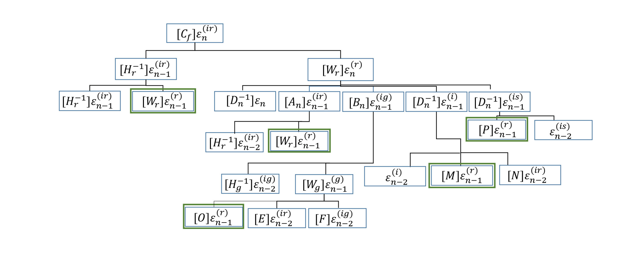
Figure 3: Tracking $\frac{\partial\bm{\varepsilon}^{(ir)}_{n}}{\partial\bm{\varepsilon}^{(r)}_{n-1}}$ terms in time

If we collect the terms to evaluate $\frac{\partial\bm{\varepsilon}^{(ir)}_{n}}{\partial\bm{\varepsilon}^{(r)}_{n-1}}$, we get

$$\begin{split}\frac{\partial\bm{\varepsilon}^{(ir)}_{n}}{\partial\bm{\varepsilon}^{(r)}_{n-1}}&=\Bigg{[}\mathbb{H}^{-1}_{r}\mathbb{W}_{r}+\mathbb{W}_{r}\mathbb{A}_{n}\mathbb{W}_{r}+\mathbb{W}_{r}\mathbb{B}_{n}\mathbb{W}_{g}\mathbb{O}+\mathbb{W}_{r}\mathbb{D}^{-1}_{n}\mathbb{M}+\mathbb{W}_{r}\mathbb{D}^{-1}_{n}\mathbb{P}\Bigg{]}\end{split}$$ (27)

Equation (27) represents term I in terms of $\varepsilon^{(ir)}_{n}$. A similar procedure is adopted for all the other six terms present in the Equation (LABEL:residual_eqn) to make a total of twenty-three terms for the coupling term $\frac{\partial\bm{R}_{n+1}}{\partial\bm{u}_{n-1}}$.

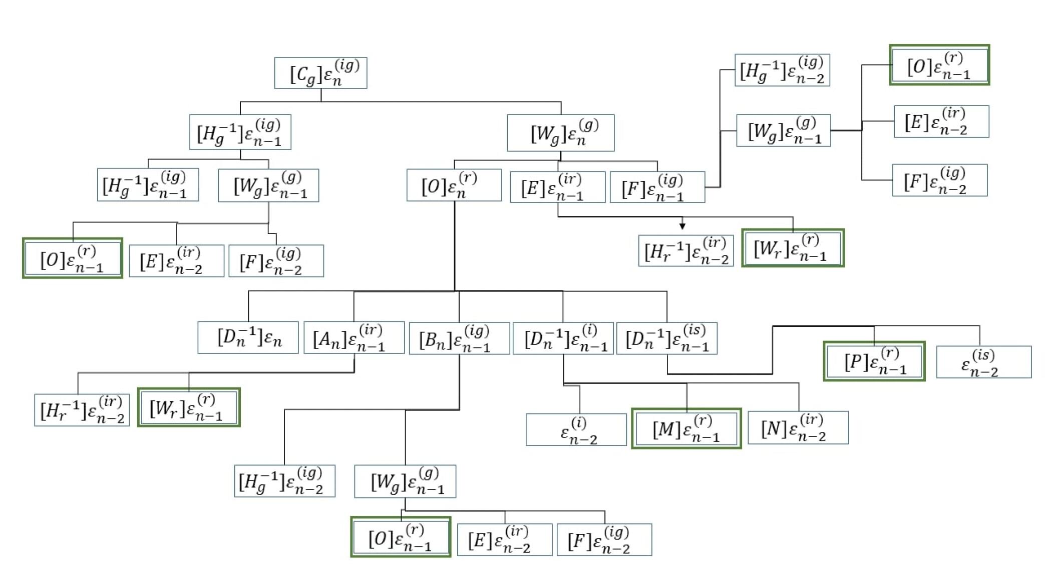
Figure 4: Tracking $\frac{\partial\bm{\varepsilon}^{(ig)}_{n}}{\partial\bm{\varepsilon}^{(r)}_{n-1}}$ terms in time

$$\frac{\partial\bm{\varepsilon}^{(ig)}_{n}}{\partial\bm{\varepsilon}^{(r)}_{n-1}}=\Bigg{[}\mathbb{H}^{-1}_{g}\mathbb{W}_{g}+\mathbb{O}_{r}+\mathbb{W}_{g}\mathbb{O}\mathbb{A}_{n}\mathbb{W}_{r}+\mathbb{W}_{g}\mathbb{O}\mathbb{B}_{n}\mathbb{W}_{g}\mathbb{O}+\mathbb{W}_{g}\mathbb{O}\mathbb{D}^{-1}_{n}\mathbb{M}+\mathbb{W}_{g}\mathbb{O}\mathbb{D}^{-1}_{n}\mathbb{P}\\ +\mathbb{W}_{g}\mathbb{E}\mathbb{W}_{r}+\mathbb{W}_{g}\mathbb{F}\mathbb{W}_{g}\mathbb{O}\Bigg{]}$$ (28)

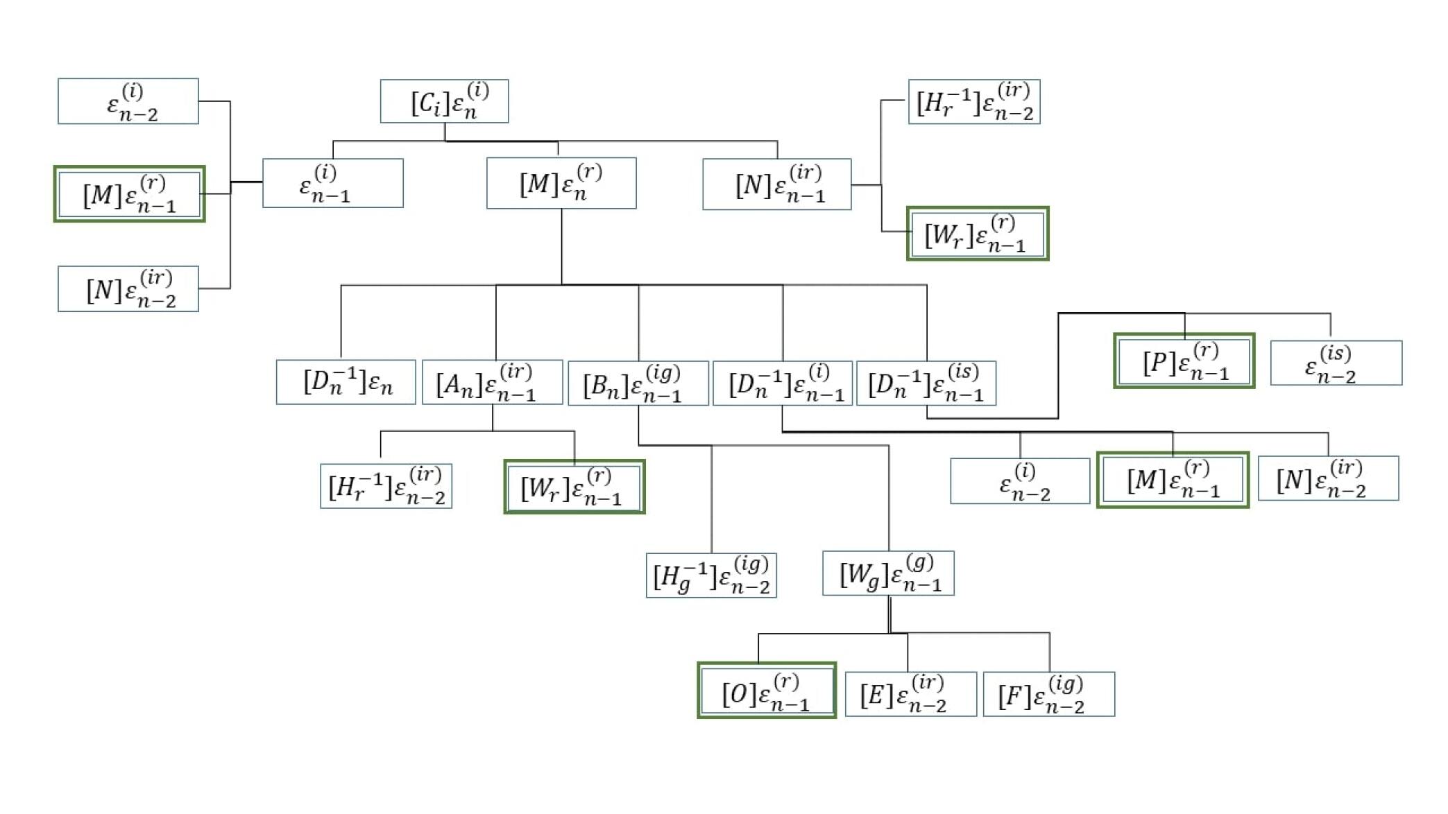
Figure 5: Tracking $\frac{\partial\bm{\varepsilon}^{(i)}_{n}}{\partial\bm{\varepsilon}^{(r)}_{n-1}}$ terms in time

$$\frac{\partial\bm{\varepsilon}^{(i)}_{n}}{\partial\bm{\varepsilon}^{(r)}_{n-1}}=\Bigg{[}\mathbb{M}+\mathbb{M}\mathbb{A}_{n}\mathbb{W}_{r}+\mathbb{M}\mathbb{B}\mathbb{W}_{g}\mathbb{O}+\mathbb{M}\mathbb{D}^{-1}_{n}\mathbb{M}+\mathbb{M}\mathbb{D}^{-1}_{n}\mathbb{P}+\mathbb{N}\mathbb{W}_{r}\Bigg{]}$$ (29)

Figure 6: Tracking $\frac{\partial\bm{\varepsilon}^{(is)}_{n}}{\partial\bm{\varepsilon}^{(r)}_{n-1}}$ terms in time

$$\frac{\partial\bm{\varepsilon}^{(is)}_{n}}{\partial\bm{\varepsilon}^{(r)}_{n-1}}=\Bigg{[}\mathbb{W}_{r}+\mathbb{P}\mathbb{A}_{n}\mathbb{W}_{r}+\mathbb{P}\mathbb{B}_{n}\mathbb{W}_{g}\mathbb{O}+\mathbb{P}\mathbb{D}^{-1}_{n}\mathbb{M}+\mathbb{P}\mathbb{D}^{-1}_{n}\mathbb{P}\Bigg{]}$$ (30)

The computation of term II is straightforward and is given by

$$\frac{\partial\bm{\varepsilon}^{(r)}_{n-1}}{\partial\bm{\varepsilon}_{n-1}}={\mathbb{D}^{-1}_{n-1}}$$ (31)

Capturing the evolution of all the components required to accurately calculate the sensitivities makes the this process computationally expensive and a highly time consuming procedure. The time taken increases exponentially with the total number of time steps required to simulate the thermo-mechanical cycle of the SMP increases. The function and the recursive algorithm used to compute the {$\frac{\partial R_{k}}{\partial u_{i}}$} terms for the total sensitivity analysis are shown in Algorithm 2 and Algorithm 3. Note that for the recursive algorithm shown in Algorithm 3, parameters $k$ and $i$ represent the time-steps. Here, the functions func_eir, func_eig, func_is, func_i are programmable versions of $\bm{\varepsilon^{(ir)}},\bm{\varepsilon^{(ig)}},\bm{\varepsilon^{(is)}},\bm{\varepsilon^{(i)}}$, shown in Equation 9[3], implemented for the $k^{th}$ step. The variable $[M]$ is a collection of parameters representing the intrinsic material properties. The function $f$ represents a general function manipulating its inputs and giving a desired output.

sens_partI($k,i,M$)

$C_{f}=f(M)$

  /* compute external variable $C_{f}$ as a function of $M$ */

/* call individual recursive functions */

$\frac{\partial\varepsilon^{(ir)}_{k}}{\partial\varepsilon^{(r)}_{i}}\leftarrow$ func_eir($C_{f},k,i,M$)

$\frac{\partial\varepsilon^{(ig)}_{k}}{\partial\varepsilon^{(r)}_{i}}\leftarrow$ func_eig($C_{f},k,i,M$)

$\frac{\partial\varepsilon^{(is)}_{k}}{\partial\varepsilon^{(r)}_{i}}\leftarrow$ func_is($C_{f},k,i,M$)

$\frac{\partial\varepsilon^{(i)}_{k}}{\partial\varepsilon^{(r)}_{i}}\leftarrow$ func_i($C_{f},k,i,M$)

term I = $f\Bigg{(}\frac{\partial\varepsilon^{(ir)}_{k}}{\partial\varepsilon^{(r)}_{i}},\frac{\partial\varepsilon^{(ig)}_{k}}{\partial\varepsilon^{(r)}_{i}},\frac{\partial\varepsilon^{(is)}_{k}}{\partial\varepsilon^{(r)}_{i}},\frac{\partial\varepsilon^{(i)}_{k}}{\partial\varepsilon^{(r)}_{i}}\Bigg{)}$

  /* term I of (23) is calculated using the output of the individual recursive functions */

term II = $f\Big{(}\frac{\partial\varepsilon^{(r)}_{i}}{\partial\varepsilon_{i}}\Big{)}$

  /* term II of (23) is calculated */

Return:$\frac{\partial R_{k}}{\partial u_{i}}\leftarrow f(\text{term I, term II})$

Algorithm 2 psuedocode to calculate the terms $\frac{\partial R_{k}}{\partial u_{i}}$ for the sensitivity evaluation

The individual functions have similar structures and one such function func_eir has been shown in details in Algorithm 3.

func_eir($C_{f},k,i,M$)

$CI=\mathbb{H}^{-1}_{r}$

  /* compute internal variable $CI$ */

$\frac{\partial\varepsilon^{(r)}_{k}}{\partial\varepsilon^{(r)}_{i}}\leftarrow$func_er($CI,k,i,M$)

  /* call function which tracks evolution of strain variables as shown in Equation (27) */

if $k>i$ then

  $\frac{\partial\varepsilon^{(ir)}_{k-1}}{\partial\varepsilon^{(r)}_{i}}\leftarrow$func_eir($C_{f}\times CI,k-1,i,M$)

  

    /* call itself with $k=k-1$ */

  

  Return:$\frac{\partial\varepsilon^{(r)}_{k}}{\partial\varepsilon^{(r)}_{i}}+\frac{\partial\varepsilon^{(ir)}_{k-1}}{\partial\varepsilon^{(r)}_{i}}$

    /* output */

Algorithm 3 Recursive algorithm to capture strain evolution with time for the sensitivity evaluation

Figure 7 gives an overview of the recursive algorithm implemented to compute $\frac{\partial\bm{R}_{k}}{\partial\bm{u}_{i}}$ for the sensitivity analysis formulation.

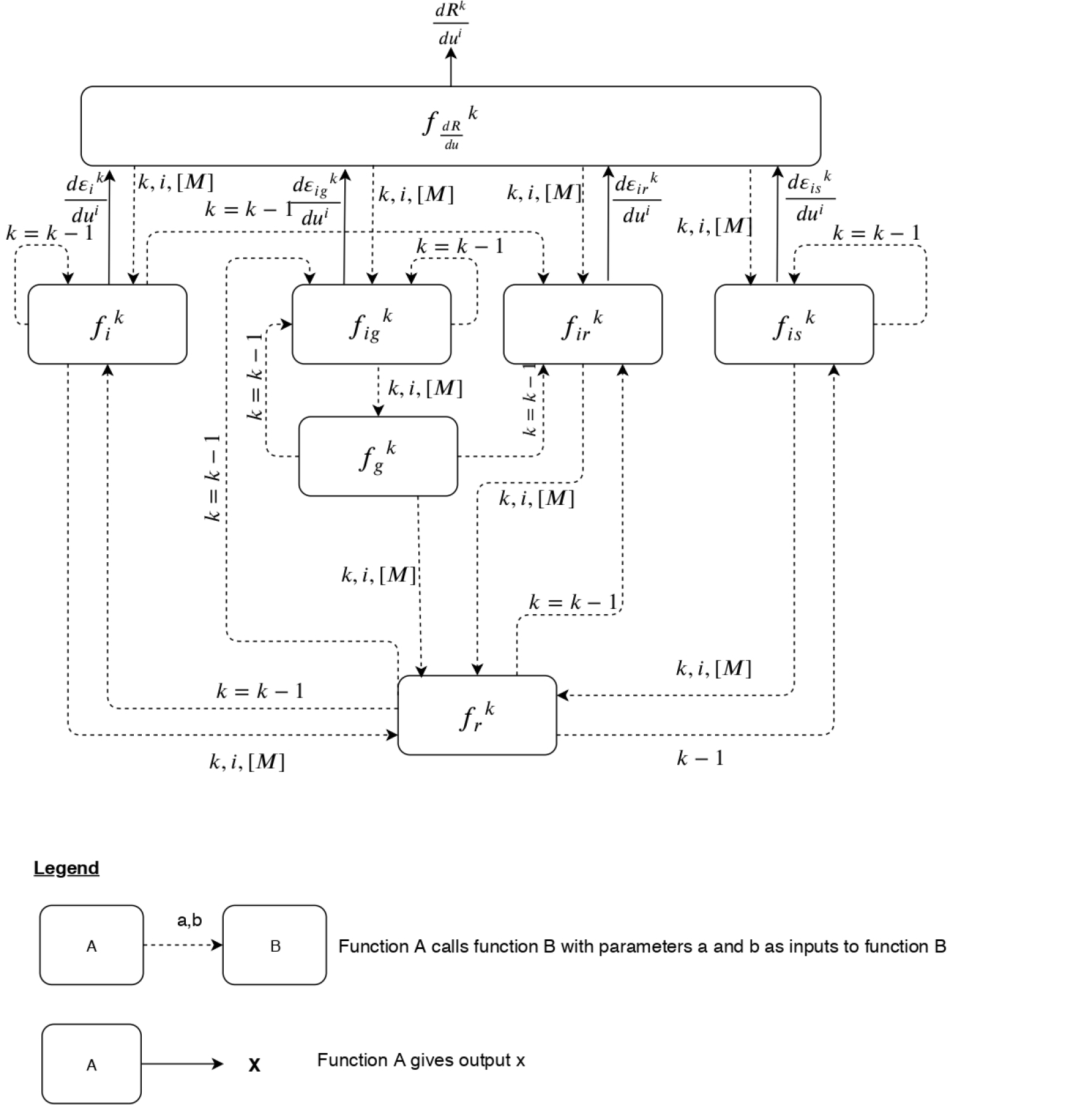
Figure 7: Recursive algorithm to calculate the terms $\frac{dR^{k}}{du^{i}}$ for the sensitivity evaluation

To verify the implementation of the sensitivity analysis, the design domain shown in Figure (2) is discretized with a coarse mesh of 45 elements. The structure is initialised with an uniform distribution of design variable $\bm{\rho}=0.3$. It was then subjected to an axial stretching load $\bm{F}=0.025\;N$ during the cooling phase of the thermo-mechanical cycle. The load was removed during the relaxation and heating phase of the thermo-mechanical programming cycle. The function of interest is the tip displacement $\bm{u}^{M}_{a}$ as shown in Equation (1). In this case, the parameter $a$ is the $y-$ degree-of-freedom of the node shown in Figure (2) and $M$ is the time step at the end of the Step-III of the thermo-mechanical programming cycle. The material parameters used for this analysis is same as listed in Table 1[3]. The adjoint method and the forward difference method were used to evaluate the derivative of the tip displacement with respect to the mixing ratio of each element. Figure (8) shows the normalised error of the sensitivity values obtained by the finite-difference approach and the adjoint sensitivity analysis. The normalised error (NE) for each element is evaluated as

$$NE=\Bigg{|}\frac{adjoint-FD}{FD}\Bigg{|}$$ (32)

Note that for elements where the sensitivity is at or near zero, we have omitted the normalized error to avoid the indication of an artificially high error due to an extremely small denominator. The displacement obtained at the end of Step-III was $-0.0130\;mm$. The maximum error between these values was found to be 2.6$\times$ $10^{-7}$. This established that the framework developed can successfully compute the sensitivities for SMP materials with a high degree of accuracy.

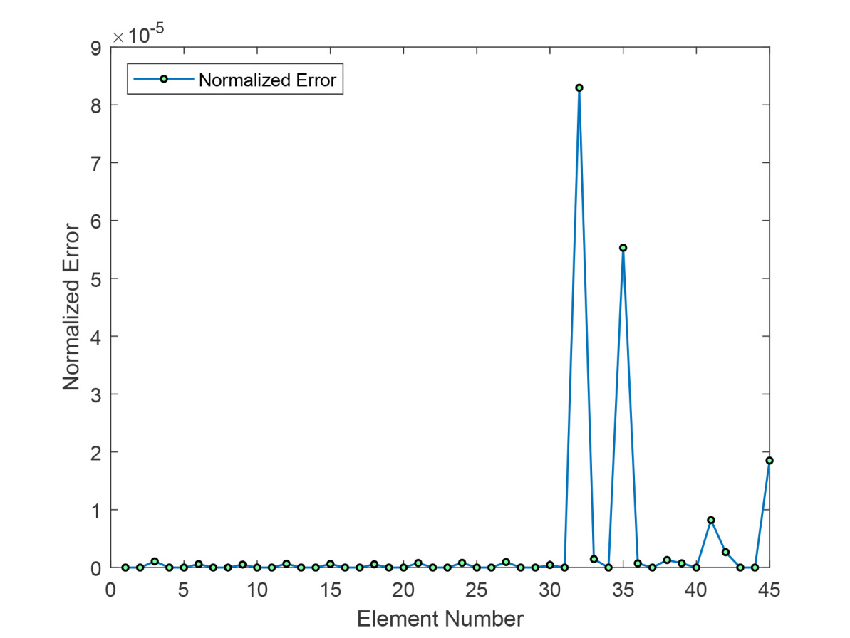
Figure 8: Comparison between the sensitivity values evaluated through the finite-difference scheme and the adjoint formulation

Figure (9) shows the time required to calculate $\frac{\partial\bm{R}_{n+1}}{\partial\bm{u}_{n-7}}$, the contribution of a total of 8 simulation steps , for a finite-element mesh of 50 elements by a single processor. As we can see, just using eight steps to simulate the entire SMP thermo-mechanical programming cycle, even for a coarse mesh can incur high computational costs. This result motivated the development of PETSc-based parallel implementation of the FEA and sensitivity evaluation framework using CPUs on the Golub Cluster at the University of Illinois. Since the bottleneck for the entire algorithm is the sensitivity evaluation and particularly the time-dependent algorithm, the parallelization is done with the objective of distributing the elements onto the processors such that each processor has the optimum number of elements for efficient computations. A total of 144 processors (6 nodes with 24 processors each) were utilized for generating the 2D results. For the 3D optimization implementation, a total of 250 processors (10 nodes with 25 processors each) were utilized.

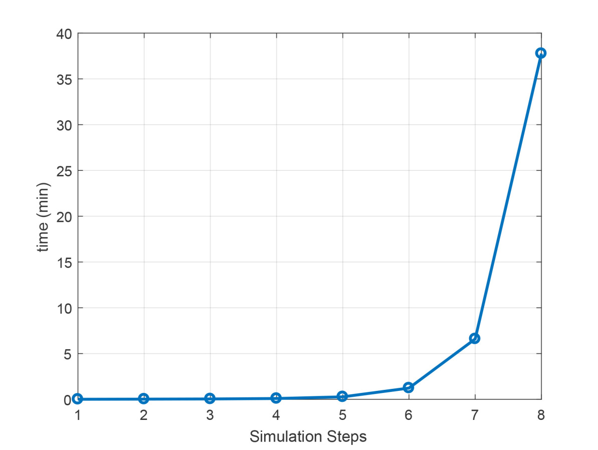
Figure 9: Computation time required for tracking $\frac{\partial\bm{\varepsilon}^{ir}_{n}}{\partial\bm{\varepsilon}^{r}_{n-1}}$ terms

Table 1: Sensitivity values evaluated through the adjoint formulation and the finite difference method.

Element No.	Adjoint Sensitivities	Finite Difference Sensitivities	Normalized Error($\times 10^{-6}$)
1	-0.2416477	-0.2416476	0.482
2	-0.0000000	-0.0000001	–
3	0.2416477	0.2416475	1.07
4	-0.2543351	-0.2543351	0.00
5	0.0000000	0.0000000	0.00
6	0.2543351	0.2543350	0.599
7	-0.2375154	-0.2375154	0.00
8	0.0000000	0.0000000	0.00
9	0.2375154	0.2375153	0.516
10	-0.2225283	-0.2225282	0.376
11	0.0000000	0.0000000	0.00
12	0.2225283	0.2225281	0.661
13	-0.2038087	-0.2038086	0.359
14	0.0000000	0.0000000	0.00
15	0.2038086	0.2038085	0.619
16	-0.1844918	-0.1844917	0.539
17	-0.0000001	-0.0000001	0.00
18	0.1844916	0.1844915	0.563
19	-0.1650572	-0.1650571	0.244
20	-0.0000010	-0.0000010	0.00
21	0.1650567	0.1650565	0.793
22	-0.1456293	-0.1456293	0.00
23	-0.0000042	-0.0000041	–
24	0.1456292	0.1456291	0.818
25	-0.1262059	-0.1262059	0.00
26	-0.0000104	-0.0000104	0.00
27	0.1262118	0.1262119	0.958
28	-0.1067716	-0.1067717	0.454
29	-0.0000017	-0.0000017	0.00
30	0.1068102	0.1068101	0.441
31	-0.0873091	-0.0873091	0.00
32	0.0001378	0.0001379	82.9
33	0.0874321	0.0874320	1.46
34	-0.0678103	-0.0678104	0.276
35	0.0008085	0.0008084	55.2
36	0.0680543	0.0680542	0.724
37	-0.0488513	-0.0488514	1.12
38	0.0027865	0.0027864	1.30
39	0.0480513	0.0480513	0.00
40	-0.0302951	-0.0302951	0.00
41	0.0042528	0.0042528	0.00
42	0.0250887	0.0250886	2.65
43	-0.0388250	-0.0388251	0.415
44	-0.0123738	-0.0123738	0.00
45	0.0027180	0.0027181	18.5

References

• [1] A. Bhattacharyya, “Hierarchical design of morphing shape-memory polymer structures via topology optimization,” Ph.D. dissertation, University of Illinois at Urbana-Champaign, 2021.
• [2] GitHub - bhttchr6/TO_ShapeMemoryPolymer: PETSc(MPI) and HPC based Finite Element Analysis and Topology Optimization for compliant gripper design with thermally-activated Shape Memory Polymers (SMP), accessed: Mar. 18, 2025. [Online]. Available: https://github.com/bhttchr6/TO_ShapeMemoryPolymer
• [3] A. Bhattacharyya and K. A. James, “Topology optimization of shape memory polymer structures with programmable morphology,” Structural and Multidisciplinary Optimization, vol. 63, no. 4, pp. 1863–1887, 2021.