Nonhermitian topological zero modes at smooth domain walls: Exact solutions

Abstract

The bulk-boundary correspondence predicts the existence of boundary modes localized at the edges of topologically nontrivial systems. The wavefunctions of hermitian boundary modes can be obtained as the eigenmode of a modified Jackiw-Rebbi equation. Recently, the bulk-boundary correspondence has been extended to nonhermitian systems, which describe physical phenomena such as gain and loss in open and non-equilibrium systems. Nonhermitian energy spectra can be complex-valued and exhibit point gaps or line gaps in the complex plane, whether the gaps can be continuously deformed into points or lines, respectively. Specifically, line-gapped nonhermitian systems can be continuously deformed into hermitian gapped spectra. Here, we find the analytical form of the wavefunctions of nonhermitian boundary modes with zero energy localized at smooth domain boundaries between topologically distinct phases, by solving the generalized Jackiw-Rebbi equation in the nonhermitian regime. Moreover, we unveil a universal relation between the scalar fields and the decay rate and oscillation wavelength of the boundary modes. This relation quantifies the bulk-boundary correspondence in nonhermitian line-gapped systems in terms of experimentally measurable physical quantities and is not affected by the details of the spatial dependence of the scalar fields. These findings shed some new light on the localization properties of boundary modes in nonhermitian and topologically nontrivial states of matter.

I Introduction

The bulk-boundary correspondence, which predicts the presence and number of localized boundary modes in relation to the topological invariants in topologically nontrivial condensed matter systems, such as topological insulators and superconductors schnyder_classification_2009 ; hasan_colloquium:_2010 ; qi_topological_2011 ; shen_topological_2011 ; shen_topological_2017 , regardless of the specific details of the physical laws governing the system hatsugai_chern_1993 ; ryu_topological_2002 ; teo_topological_2010 . However, only the specific form of these laws can accurately describe the local physical properties of these excitations, such as their localization and spatial behavior. Generalizations of the bulk-boundary correspondence apply to nonhermitian systems ashida_non-hermitian_2020 ; okuma_non-hermitian_2023 as well. Nonhermitian Hamiltonians naturally describe a variety of physical systems, such as open systems in the presence of gain and loss mechanisms, or dissipation, and exhibit the presence of complex energy spectra shen_topological_2018 ; gong_topological_2018 ; kawabata_symmetry_2019 ; ashida_non-hermitian_2020 ; okuma_non-hermitian_2023 ; schindler_hermitian_2023 ; nakamura_bulk-boundary_2024 in several different condensed matters and metamaterials gao_observation_2015 ; ghatak_observation_2020 ; zhang_observation_2021 ; su_direct_2021 ; fleckenstein_non-hermitian_2022 ; lin_observation_2022 ; liu_experimental_2023 ; wang_non-hermitian_2023 ; ochkan_non-hermitian_2024 . A fundamental distinctions in this case is between spectra with line gaps and point gaps shen_topological_2018 ; gong_topological_2018 ; kawabata_symmetry_2019 . Point gaps describe energy eigenvalues that do not cross a reference point (usually the origin at zero), while line gaps describe energy eigenvalues that do not cross a reference line in the complex plane. Any nonhermitian Hamiltonian with line gaps can be adiabatically deformed into a corresponding hermitian hamiltonian with conventional energy gaps. Hence, the bulk-boundary correspondence and the definition of topological invariants can be directly extended in this case. Hermitian Hamiltonians with nontrivial topology are naturally described by a modified Jackiw-Rebbi equation shen_topological_2011 ; shen_topological_2017 , which is a spinorial second-order linear differential equation, which generalized the original Jackiw-Rebbi equation jackiw_solitons_1976 , which is a spinorial first-order linear differential equation. Henceforth, nonhermitian hamiltonians can be described by a nonhermitian version of the modified Jackiw-Rebbi equation with complex coefficients.

In recent works, we derived the analytical solutions of the modified Jackiw-Rebbi equation describing zero energy boundary modes at smooth domain walls between topological trivial and nontrivial phases in the hermitian regime marra_topological_2024 and extended some of these findings to the nonhermitian regime marra_zero_2025 . In this work, we derive the analytical form of the wavefunctions of zero modes in nonhermitian line-gapped systems described by a modified Jackiw-Rebbi equation with space-dependent mass and velocity terms, allowing for complex coefficients. The space dependency describes the case of a smooth domain wall, i.e., the case where the nonuniform space dependence is confined in a region of finite length $w$. This allows us to derive the bulk-boundary correspondence for nonhermitian line-gapped systems by directly establishing the correspondence between the nonhermitian topological invariant and the asymptotic decay rate of the zero modes. We thus analyze several properties of these zero modes, such as the localization length $\xi$, oscillation wavelength $\lambda$, conditions for the reality of the wavefunction, local properties, and local topological invariant, and show specific examples of nonhermitian zero modes corresponding to different regimes. This allows us to distinguish between qualitatively different cases: featureless zero modes in the limit $w\to 0$, having "no hair" (in analogy with other featureless objects such as black holes); non-featureless zero modes in the regime $\xi,\lambda>w>0$, having "short hair" (i.e., effectively featureless at long length scales); non-featureless zero modes in the regime $w>\xi,\lambda>0$ having "long hair" (i.e., being nonfeatureless at all length scales). We also discuss possible experimental signatures of the bulk-boundary correspondence by unveiling a universal relation between the local properties of the zero modes (localization length and oscillations wavelength $\lambda$) and bulk physical quantities.

II Zero modes: Exaxt solutions

II.1 The modified Jackiw-Rebbi equation in the nonhermitian regime

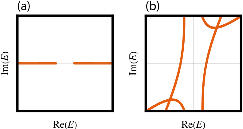
Figure 1: Energy spectra of the generalized Jackiw-Rebbi equation with uniform fields $v(x)=v$, $m(x)=m$ in Eq.˜4. (a) Hermitian case with $v,m\in\mathbb{R}$ corresponding to a real energy spectrum with an energy gap. (b) nonhermitian case with $v,m\notin\mathbb{R}$ corresponding to a complex energy spectrum with a line gap.

The Jackiw-Rebbi equation jackiw_solitons_1976 is a Dirac equation where the mass term is space-dependent. Here, we consider a generalization of the Jackiw-Rebbi equation, where both the mass and Dirac velocity are space-dependent, and with an additional quadratic term in the momentum given by

$$\left[\left(\eta p^{2}+{m}(x)\right)\sigma_{z}+{2{v}}(x)p\,\sigma_{y}\right]\Psi(x)=E\Psi(x).$$ (1)

where $\Psi(x)^{\dagger}=[\psi(x)^{\dagger},\psi(x)]$ is the fermionic field, $\sigma_{xyz}$ the Pauli matrices, $p=-\mathrm{i}\partial$ the momentum operator, $\eta\geq 0$. Furthermore, we consider here the nonhermitian case where the fields are complex-valued ${m}(x),{v}(x)\in\mathbb{C}$. This equation can be interchangeably referred to as a modified Jackiw-Rebbi equation or a modified Dirac equation with space-dependent mass and Dirac velocity. The hermitian case ${m}(x),{v}(x)\in\mathbb{R}$ describes topological insulators and superconductors and has been studied at length in our previous work Ref. marra_topological_2024, . Here, we will address the cases where $\mathrm{Im}({m}(x))\neq 0$ or $\mathrm{Im}({v}(x))\neq 0$, which generalize the equation above to the nonhermitian case. The nonhermitian case $\mathrm{Im}({m}(x))\neq 0$ may describe, e.g., a topological insulator or superconductor subject to a nonhermitian potential $V(x)={m}(x)$, while $\mathrm{Im}({v}(x))\neq 0$ may describe, e.g., a topological superconductor with a nonhermitian superconducting order parameter describing dissipation effects on Cooper pairs. We will consider the zero modes $E=0$ on infinite or semi-infinite intervals that are normalizable and satisfy Dirichlet boundary conditions. The zero modes of the generalized Jackiw-Rebbi equation in Eq.˜1 are eigenstates of $\sigma_{x}$, i.e.,

$$\Psi(x)\propto\begin{pmatrix}1\\ s\end{pmatrix}\varphi(x),\,\,\sigma_{x}\Psi(x)=s\Psi(x),$$ (2)

for $s=\pm 1$ and with $\varphi(x)$ satisfying

$$\varphi^{\prime\prime}(x)+{2s{v}}(x)\varphi^{\prime}(x)-{m}(x)\varphi(x)=0,$$ (3)

where we absorbed $\eta$ by redefining the fields ${v}(x)\to{v}(x)/\eta$ and ${m}(x)\to{m}(x)/\eta$. We refer to the eigenvalue $s=\pm 1$ as the pseudospin. Notice that, if $\mathrm{Im}({m}(x))\neq 0$ or $\mathrm{Im}({v}(x))\neq 0$, the equation is not real and does not have real solutions in the general case. We recall that real wavefunctions are the hallmark of Majorana zero modes. In other words, the zero modes of a nonhermitian system are not necessarily Majorana zero modes.

II.2 Line gap nonhermitian topology

Assuming uniform fields $v(x)=v$, $m(x)=m$, the Hamiltonian in Eq.˜1 becomes diagonal in the momentum eigenfunctions and can be written as

$$\left(\left(k^{2}+{m}\right)\sigma_{z}+{2{v}}k\,\sigma_{y}\right)\Psi(k)=E\Psi(k),$$ (4)

with an energy spectra given by $E(k)^{2}=(k^{2}+m)^{2}+4v^{2}k^{2}$. In the nonhermitian case, the energy spectra are generally complex. In nonhermitian systems shen_topological_2018 ; gong_topological_2018 ; kawabata_symmetry_2019 , energy spectra can exhibit either point gaps, where the energy eigenvalues do not cross a specific point in the complex plane, or line gaps, where the energy eigenvalues do not cross a specific line in the complex plane. nonhermitian spectra with line gaps can always be adiabatically deformed to hermitian and gapped spectra. The nonhermitian complex energy spectra of Eq.˜4 shows a line gap, which is the line in the complex plane with $\mathrm{Im}(E(k))=0$, and can be deformed to hermitian real energy spectra with an energy gap by taking the limits $\mathrm{Im}(v)\to 0$, $\mathrm{Im}(m)\to 0$, as shown in Fig.˜1. The line gap closes when $E(k)=0$ for some momenta $k\in\mathbb{R}$. Hence, the closing of the line gap is determined if the condition $E(k)=0$ is satisfied for any $k\in\mathbb{R}$, i.e., if any of the solutions of the algebraic equation $(k^{2}+m)^{2}+4v^{2}k^{2}=0$, which are given by $k=\pm\sqrt{-\left(\sqrt{m+v^{2}}\pm\sqrt{v^{2}}\right)^{2}}$, is real. This condition is satisfied only if $\mathrm{Re}\left(\sqrt{m+v^{2}}\pm\sqrt{v^{2}}\right)=0$. Hence, the line gap of the complex energy spectra closes when the quantity

$$M=|\mathrm{Re}(\sqrt{{v}^{2}+{m}})|-|\mathrm{Re}({{v}})|,$$ (5)

becomes zero. The closing of the line gap separates topologically nonequivalent phases with $M>0$ and $M<0$. In the hermitian limit, one has that $M=0$ if and only if $m=0$, and therefore, the condition above simply reduces to the condition $m=0$. To determine the topological invariant $W$ of the gapped spectra, we recall that in the hermitian case, the topologically trivial phase with $W=0$ corresponds to $m>0$, and the topologically nontrivial phases with $W\neq 0$ correspond to $m<0$ with $W=\operatorname{sgn}(v)$. Since the nonhermitian topological invariant must coincide with the hermitian topological invariant in the limit $\mathrm{Im}(v)\to 0$, $\mathrm{Im}(m)\to 0$, one can conclude that

$$W=\begin{cases}\operatorname{sgn}(\mathrm{Re}({v})),&\text{ if }\operatorname{sgn}({M})=-1\text{ or }0,\\ 0&\text{ if }\operatorname{sgn}({M})=1.\end{cases}$$ (6)

II.3 Exact solutions of zero modes at smooth domain walls

We assume that the fields become constant at large distances $x\to\pm\infty$ and that they approach their asymptotic values exponentially as $|{m}(x\to\mp\infty)-{m}_{L,R}|\sim{e}^{-|x|/w}$, $|{v}(x\to\mp\infty)-{v}_{L,R}|\sim{e}^{-|x|/w}$. Here, the constant $w>0$ is a characteristic length that measures the width of the smooth domain wall localized at the origin $x=0$. Under these very general assumptions, by mapping the whole real line $-\infty<x<\infty$ into the finite segment $0<y<1$ with the substitution $y(x)=(1+\tanh{(x/2w)})/2$, we found that for a given pseudospin $s=\pm 1$, the general solution of the modified Jackiw-Rebbi equation is given by a linear combination $A_{1}\varphi_{1}^{s}(x)+A_{2}\varphi_{2}^{s}(x)$ where

$$\varphi_{1,2}^{s}(x) =y(x)^{{w\alpha_{L}^{\pm}}}(1-y(x))^{{w\alpha_{R}^{\mp}}}F_{1,2}(y(x))$$

$$=\frac{{e}^{({\alpha_{L}^{\pm}}-{\alpha_{R}^{\mp}})x/2}}{\left(2\cosh{(x/2w)}\right)^{{w(\alpha_{L}^{\pm}}+{\alpha_{R}^{\mp}})}}F_{1,2}(x),$$ (7)

with exponents $\alpha_{L}^{\pm}=-s{{v}}_{L}\pm{q}_{L}$, $\alpha_{R}^{\pm}=s{{v}}_{R}\pm{q}_{R}$, where ${q}_{L,R}=\sqrt{{v}_{L,R}^{2}+{m}_{L,R}}$, which depend only on the values of the fields at large distances $|x|\gg w$, and where the functions $F_{1,2}$ are bounded or diverge polynomially for $x\to\pm\infty$. The detailed derivation of these solutions is given in Appendix˜A. Asymptotically, these solutions give

$$\varphi_{1,2}^{s}(x\to-\infty) \sim{e}^{-\alpha_{L}^{\pm}|x|}={e}^{-\mu_{L}^{\pm}|x|}{e}^{-\mathrm{i}\kappa_{L}^{\pm}|x|},$$ (8a)

$$\varphi_{1,2}^{s}(x\to+\infty) \sim{e}^{-\alpha_{R}^{\mp}|x|}={e}^{-\mu_{R}^{\mp}|x|}{e}^{-\mathrm{i}\kappa_{R}^{\mp}|x|},$$ (8b)

where $\mu_{L,R}^{\pm}=1/\xi_{L,R}^{\pm}=\mathrm{Re}(\alpha_{L,R}^{\pm})$ are the decay rates and decay lengths, while $\kappa_{L,R}^{\pm}=2\pi/\lambda_{L,R}^{\pm}=\mathrm{Im}(\alpha_{L,R}^{\pm})$ the momentum and wavelengths describing the oscillatory behavior of the solutions. Obviously $\mu_{L,R}^{+}=\mu_{L,R}^{-}=\mp s\mathrm{Re}({v}_{L,R})$ if $\mathrm{Re}({q}_{L,R})=0$ and $\kappa_{L,R}^{+}=-\kappa_{L,R}^{-}=\mathrm{Im}({q}_{L,R})$ if $\mathrm{Im}({v}_{L,R})=0$. If the system becomes asymptotically hermitian for $x\to\mp\infty$, i.e., $\mathrm{Im}({m}_{L,R})=\mathrm{Im}({v}_{L,R})=0$ for $x\to\mp\infty$, then $\kappa_{L,R}^{+}=\kappa_{L,R}^{-}=0$ for ${{v}}_{L,R}^{2}+{m}_{L,R}\geq 0$, with $\mu_{L,R}^{+}=\mu_{L,R}^{-}$ for ${{v}}_{L,R}^{2}+{m}_{L,R}=0$, while $\mu_{L,R}^{+}=\mu_{L,R}^{-}=\mp s{v}_{L,R}$ and $\kappa_{L,R}^{+}=-\kappa_{L,R}^{-}=\mathrm{Im}({q}_{L,R})\neq 0$ for ${{v}}_{L,R}^{2}+{m}_{L,R}<0$.

Let us assume now that the fields ${v}(x)$ and ${m}(x)$ can be expanded in powers of $y(x)$ up to the first and second order, respectively, i.e., as ${v}(x)={v}_{0}+{v}_{1}y(x)$, and ${m}(x)={m}_{0}+{m}_{1}y(x)+{m}_{2}y(x)^{2}$, where the coefficients of the expansion are given by $v_{0}=v_{L}$, ${v}_{1}={v}_{R}-{v}_{L}$, and $m_{0}=m_{L}$, $m_{1}+m_{2}={m}_{R}-{m}_{L}$, ${m}_{2}=2({m}_{L}+{m}_{R})-4{m}(0)$. In this case, we found that the general solution of the modified Jackiw-Rebbi equation can be written in terms of hypergeometric functions. Indeed, for a given pseudospin $s=\pm 1$, we found that

$$F_{1,2}(x)= {{{\,}_{2}F_{1}}\left(a_{1,2},b_{1,2},c_{1,2},\tfrac{1}{{e}^{\mp\,x/w}+1}\right)},$$ (9)

where ${{\,}_{2}F_{1}}(a,b,c,y)$ is the hypergeometric function with

$$a_{1,2} =\pm w\left({{q}_{L}}-{{q}_{R}}\right)+\tfrac{1}{2}+\tfrac{1}{2}{\sqrt{\left(2ws{v}_{1}-1\right)^{2}+4w^{2}{m}_{2}}}$$ (10a)

$$b_{1,2} =\pm w\left({{q}_{L}}-{{q}_{R}}\right)+\tfrac{1}{2}-\tfrac{1}{2}{\sqrt{\left(2ws{v}_{1}-1\right)^{2}+4w^{2}{m}_{2}}}$$ (10b)

$$c_{1,2} =1+2w{q}_{L,R},$$ (10c)

assuming $c_{1,2}-a_{1,2},c_{1,2}-b_{1,2}\notin\mathbb{Z}_{\leq}$ (we denote $\mathbb{Z}_{\leq}$ the set of nonpositive integers). The detailed derivation of this solution is given in Appendix˜B. These solutions generalize to the nonhermitian case the solutions derived in Ref. marra_topological_2024, . The asymptotic behavior of the functions $F_{1,2}$ is summarized in Table˜1. If either $c_{1}-a_{1}=c_{2}-a_{2}\in\mathbb{Z}_{\leq}$ or $c_{1}-b_{1}=c_{2}-b_{2}\in\mathbb{Z}_{\leq}$, the solutions of the hypergeometric equation become more complicated, since some of the hypergeometric functions become linearly dependent or ill-behaved for $x\to\pm\infty$. We will not address these cases explicitly in this work.

Table 1: The asymptotic behavior of the functions $F_{1,2}$. We assume $c_{1,2}-a_{1,2},c_{1,2}-b_{1,2}\notin\mathbb{Z}_{\leq}$. In the case ${m}_{L,R},{v}_{L,R}\in\mathbb{R}$ one has $\mathrm{Re}({q}_{L,R})>0$ if ${{v}}_{L,R}^{2}+{m}_{L,R}>0$, and $\mathrm{Re}({q}_{L,R})=0$ if ${{v}}_{L,R}^{2}+{m}_{L,R}\leq 0$.

The solutions $\varphi_{1,2}^{s}(x)$ simplify in the cases where $|{v}_{L,R}|={v}$ or ${m}_{L,R}={m}$ or if the fields are uniform, as shown in Table I of Ref. marra_topological_2024, . Since the functions $F_{1,2}$ are bounded or diverge polynomially, as summarized in Table˜1, the exponents $\alpha_{L}^{\pm}$ and $\alpha_{R}^{\pm}$ uniquely determine the asymptotic behavior of the solutions. Hence, the existence of zero modes, i.e., particular solutions that are normalizable and satisfy the boundary conditions on a given interval, is uniquely and solely determined by the exponents $\alpha_{L}^{\pm}$ and $\alpha_{R}^{\pm}$. Since these exponents only depend on $v_{L,R}$, $m_{L,R}$, one can infer that the values of the fields at large distances and the boundary conditions univocally determine the existence and number of zero modes and their pseudospin $s$ on infinite and semi-infinite intervals.

III Nonhermitian bulk-boundary correspondence

III.1 Topological invariant

In hermitian systems, the bulk-boundary correspondence hatsugai_chern_1993 ; ryu_topological_2002 ; teo_topological_2010 establishes a relation between the number of topologically protected modes at the boundary between two topologically inequivalent phases. For uniform and hermitian fields $m(x)=m\in\mathbb{R}$, $v(x)=v\in\mathbb{R}$, one can define the topological invariant $W\in\mathbb{Z}_{2}$ characterizing the Hamiltonian as $W=\operatorname{sgn}(v)$ for $m\leq 0$ and $W=0$ otherwise kitaev_unpaired_2001 . Hence, assuming uniform fields at the asymptotes $x\to\pm\infty$, the phase on the left $x\ll-w$ has topological invariant $W_{L}=\operatorname{sgn}(v_{L})$ if $m_{L}\leq 0$ and $v_{L}\neq 0$, and $W_{L}=0$ otherwise. Analogously, the phase on the right $x\gg w$ gives $W_{R}=\operatorname{sgn}(v_{R})$ if $m_{R}\leq 0$ and $v_{R}\neq 0$, and $W_{R}=0$ otherwise (see Refs. kitaev_unpaired_2001 ; shen_topological_2011 ). The number of topologically protected zero-energy modes localized at the boundary is equal to the difference between the values of the topological invariant on the right and on the left of the boundary $\Delta W=|W_{L}-W_{R}|$.

Here, we want to generalize the bulk-boundary correspondence to nonhermitian systems, particularly to nonhermitian systems described by nonhermitian modified Jackiw-Rebbi equations as in Eq.˜1. These nonhermitian systems can be seen as an adiabatical "deformation" of the conventional hermitian systems. Hence, the bulk gap of the hermitian Hamiltonian is transformed into a line gap in the nonhermitian case schindler_hermitian_2023 . We will define here a topological invariant for these nonhermitian Hamiltonians by an adiabatic deformation of the topological invariant in the hermitian case, justified by our analysis of the decay rates of the localized boundary modes solutions of the Jackiw-Rebbi equations in Eq.˜1.

To determine the existence, number, and asymptotic properties of the zero modes, in agreement with our previous considerations on the line gap nonhermitian topology and the definition of bulk topological invariant in Eq.˜6, we define

$${M}_{L,R}= |\mathrm{Re}(\sqrt{{v}_{L,R}^{2}+{m}_{L,R}})|-|\mathrm{Re}({{v}}_{L,R})|=$$

$$|\mathrm{Re}({q}_{L,R})|-|\mathrm{Re}({{v}}_{L,R})|,$$ (11a)

$${K}_{L,R}= |\mathrm{Im}(\sqrt{{v}_{L,R}^{2}+{m}_{L,R}})|+|\mathrm{Im}({{v}}_{L,R})|=$$

$$|\mathrm{Im}({q}_{L,R})|+|\mathrm{Im}({{v}}_{L,R})|,$$ (11b)

$$W_{L,R}= \begin{cases}\operatorname{sgn}(\mathrm{Re}({v}_{L,R})),&\text{ if }\operatorname{sgn}({M}_{L,R})=-1\text{ or }0,\\ 0&\text{ if }\operatorname{sgn}({M}_{L,R})=1,\end{cases}$$ (11c)

where we use the common convention $\operatorname{sgn}(0)=0$. We will refer to $W_{L,R}$ and $M_{L,R}$ as the (nonhermitian) topological invariant and the (nonhermitian) topological mass on the left and right side of the smooth domain wall, respectively. These quantities depend only on the values of the fields ${m}_{L,R}$ and ${v}_{L,R}$ at large distances $|x|>w$. For the asymptotically hermitian case $\mathrm{Im}({m}_{L,R})=\mathrm{Im}({v}_{L,R})=0$, one has that $\operatorname{sgn}({M}_{L,R})=\operatorname{sgn}({m}_{L,R})$, ${K}_{L,R}=|\mathrm{Im}({q}_{L,R})|$, and ${W}_{L,R}=\operatorname{sgn}({v}_{L,R})$ for ${m}_{L,R}\leq 0$ and ${W}_{L,R}=0$ otherwise. Hence, our definitions of nonhermitian topological mass $M_{L,R}$ and nonhermitian topological invariant $W_{L,R}$ in Eqs.˜11 and 11c reduces to the usual definition of topological mass and topological invariant in the hermitian case.

To demonstrate the relations between the (nonhermitian) topological invariants $W_{L,R}$ and the existence and number of zero modes, we start to analyze the asymptotic behavior of the solutions of the Jackiw-Rebbi equation. Since the two solutions decay as $|\varphi_{1,2}^{s}(x\to-\infty)|={e}^{\mathrm{Re}(\alpha_{L}^{\pm})x}$ and $\varphi_{1,2}^{s}(x\to+\infty)={e}^{-\mathrm{Re}(\alpha_{R}^{\mp})x}$, the boundary conditions on the left are satisfied when $\mathrm{Re}(\alpha_{L}^{\pm})>0$ while the boundary conditions on the right are satisfied when $\mathrm{Re}(\alpha_{R}^{\mp})>0$, respectively for the two solutions $\varphi_{1,2}^{s}(x)$. To determine whether the solutions satisfy the boundary conditions, we thus need to study the sign of the exponents $\mathrm{Re}(\alpha_{L,R}^{\pm})$. For ${m}_{L},{v}_{L}\in\mathbb{C}$, these exponents are completely determined by the quantities ${M}_{L}$ and ${K}_{L}$, since

$$\operatorname{sgn}(\mathrm{Re}(\alpha_{L}^{\pm}))=\left\{\begin{array}[]{ll}\pm 1,&\text{ for }{M}_{L}>0,\\ 0\text{ or }-sW_{L},&\text{ for }{M}_{L}=0,\\ -sW_{L},&\text{ for }{M}_{L}<0.\end{array}\right.$$ (12)

In the first case, the solution $\varphi_{1}^{s}(x)$ decays while the solution $\varphi_{2}^{s}(x)$ diverges for $x\to-\infty$. In the second case, one of the solutions $\varphi_{1,2}^{s}(x)$ converges to a constant value. In the last case, both solutions $\varphi_{1,2}^{s}(x)$ decays for $x\to-\infty$ as long as $s=-\operatorname{sgn}(\mathrm{Re}({v}_{L}))$. Analogous statements hold for $\alpha_{R}^{\pm}$ by exchanging left and right ${v}_{L}\to{v}_{R}$, ${m}_{L}\to{m}_{R}$, $W_{L}\to W_{R}$, ${M}_{L}\to{M}_{R}$, and $s\to-s$.

We are now ready to demonstrate the nonhermitian generalization of the bulk-boundary correspondence. To do so, we will demonstrate that the number of localized zero-energy modes in the interval $-\infty<x<\infty$ (infinite system) equals $|W_{L}-W_{R}|$, and that the number of localized zero-energy modes in the interval $0\leq x<\infty$ (semi-infinite system) is equal to $|W_{R}|$.

III.2 Infinite interval $-\infty<x<\infty$

Zero modes on the interval $-\infty<x<\infty$ satisfying the boundary conditions $\varphi(\pm\infty)=0$ are given by the modes $\varphi_{1,2}^{s}(x)$ in Eq.˜7 with $\mathrm{Re}(\alpha_{L}^{\pm})>0$ and $\mathrm{Re}(\alpha_{R}^{\pm})>0$. In this case, there exists $|W_{L}-W_{R}|$ zero modes, i.e., there are two independent modes if $W_{L}W_{R}=-1$, one independent mode if $W_{L}=\pm 1$ and $W_{R}=0$ or if $W_{R}=\pm 1$ and $W_{L}=0$. To demonstrate these statements, we need to find the particular solutions that satisfy $\varphi(x\to\pm\infty)=0$, i.e., $\varphi(y\to 0)=\varphi(y\to 1)=0$. Assuming $|F_{1,2}(y)|$ convergent or logarithmically divergent at $y=0,1$, we need to care about the factors $y^{w\alpha_{L}^{-}}$ and $(1-y)^{w\alpha_{R}^{-}}$, which converge to zero at $y=0$ and $y=1$ only if $\mathrm{Re}({\alpha_{L}^{-}})>0$ and $\mathrm{Re}({\alpha_{R}^{-}})>0$, respectively. This gives only four possible outcomes, discussed below and summarized in Table˜2.

III.2.1 Two zero modes for $W_{L}W_{R}=-1$

For $\operatorname{sgn}({M}_{L})=\operatorname{sgn}({M}_{R})=-1$, and $\mathrm{Re}({v}_{L})\mathrm{Re}({v}_{R})<0$, the topological invariants are opposite and nonzero $W_{L}W_{R}=-1$. Moreover, in this case, one has $\operatorname{sgn}(\mathrm{Re}(\alpha_{L}^{\pm}))=-s\operatorname{sgn}(\mathrm{Re}({v}_{L}))$ and $\operatorname{sgn}(\mathrm{Re}(\alpha_{R}^{\pm}))=s\operatorname{sgn}(\mathrm{Re}({v}_{R}))$, which gives $\operatorname{sgn}(\mathrm{Re}(\alpha_{L}^{\pm}))=\operatorname{sgn}(\mathrm{Re}(\alpha_{R}^{\pm}))$ in this case. Choosing the pseudospin $s=\operatorname{sgn}{(\mathrm{Re}({v}_{L}))}=-\operatorname{sgn}{\mathrm{Re}(({v}_{R}))}$ gives $\mathrm{Re}(s{v}_{L})>0$ and $\mathrm{Re}(s{v}_{R})<0$ and therefore $\mathrm{Re}(\alpha_{L}^{\pm}),\mathrm{Re}(\alpha_{R}^{\pm})<0$: In this case, the two linearly independent solutions $\varphi_{1,2}^{s}(x)$ in Eq.˜42 diverge exponentially with different decaying lengths at $x\to\pm\infty$, and their linear combination cannot satisfy the boundary conditions. Choosing instead the opposite pseudospin $s=-\operatorname{sgn}{(\mathrm{Re}({v}_{L}))}=\operatorname{sgn}{(\mathrm{Re}({v}_{R}))}$ gives $\mathrm{Re}(s{v}_{L})<0$ and $\mathrm{Re}(s{v}_{R})>0$ and therefore $\mathrm{Re}(\alpha_{L}^{\pm}),\mathrm{Re}(\alpha_{R}^{\pm})>0$: In this case, the two solutions $\varphi_{1,2}^{s}(x)$ decay exponentially to zero for $x\to\pm\infty$. Therefore, the particular solution satisfying the boundary conditions is any linear combination

$$\varphi(x)=A_{1}\varphi_{1}^{s}(x)+A_{2}\varphi_{2}^{s}(x),$$ (13)

up to normalization constants $A_{1,2}$, with pseudospin $s=-\operatorname{sgn}{(\mathrm{Re}({v}_{L}))}=\operatorname{sgn}{(\mathrm{Re}({v}_{R}))}$ in Eq.˜2, $\varphi_{1,2}^{s}(x)$ as in Eqs.˜42 and 57, and ${\alpha_{L}}$, ${\alpha_{R}}$ given by Eq.˜37. Since $\mathrm{Re}(\alpha_{L,R}^{-})\leq\mathrm{Re}(\alpha_{L,R}^{+})$, the asymptotic behavior at large distances is given by

$$\varphi(x\to-\infty) \sim{e}^{+\alpha_{L}^{-}x}={e}^{+\mu_{L}^{-}x}{e}^{+\mathrm{i}\kappa_{L}^{-}x},$$ (14)

$$\varphi(x\to+\infty) \sim{e}^{-\alpha_{R}^{-}x}={e}^{-\mu_{R}^{-}x}{e}^{-\mathrm{i}\kappa_{R}^{-}x},$$ (15)

where $\mu_{L,R}^{-}=\mathrm{Re}(\alpha_{L,R}^{-})=-{M}_{L,R}$.

The asymptotic behavior of the modes $\varphi_{1}^{s}$ and $\varphi_{2}^{s}$ are determined on the left side by the exponents $\alpha_{L}^{+}=-s{v}_{L}+{q}_{L}$ (characteristic lengths $\xi_{L}^{+}$, $\lambda_{L}^{+}$) and $\alpha_{L}^{-}=-s{v}_{L}-{q}_{L}$ (characteristic lengths $\xi_{L}^{-}$, $\lambda_{L}^{-}$), respectively, and on the right side by the exponents $\alpha_{R}^{-}=s{v}_{R}-{q}_{R}$ (characteristic lengths $\xi_{R}^{-}$, $\lambda_{R}^{-}$) and $\alpha_{R}^{+}=s{v}_{R}+{q}_{R}$ (characteristic lengths $\xi_{R}^{+}$, $\lambda_{R}^{+}$), respectively.

III.2.2 One zero mode for $W_{L}=0$, $W_{R}=\pm 1$

For $\operatorname{sgn}({M}_{L})=1$, $\operatorname{sgn}({M}_{R})=-1$, and $\mathrm{Re}({v}_{R})\neq 0$, the topological invariants are $W_{L}=0$ and $W_{R}=\operatorname{sgn}(\mathrm{Re}({v}_{R}))=\pm 1$. Moreover, in this case, one has $\operatorname{sgn}(\mathrm{Re}(\alpha_{R}^{\pm}))=s\operatorname{sgn}(\mathrm{Re}({v}_{R}))$ and $\mathrm{Re}(\alpha_{L}^{+})>0>\mathrm{Re}(\alpha_{L}^{-})$. Choosing $s=-\operatorname{sgn}(\mathrm{Re}({v}_{R}))$ gives $\mathrm{Re}(\alpha_{R}^{\pm})<0$, and therefore the two linearly independent solutions $\varphi_{1,2}^{s}(x)$ in Eq.˜42 respectively decay to zero and diverge for $x\to-\infty$ and both diverge for $x\to\infty$, and thus their linear combination cannot satisfy the boundary conditions. Choosing instead $s=\operatorname{sgn}(\mathrm{Re}({v}_{R}))$ gives $\mathrm{Re}(\alpha_{R}^{\pm})>0$, and therefore the solution $\varphi_{1}^{s}(x)$ now decays to zero for $x\to\pm\infty$, while $\varphi_{2}^{s}(x)$ still diverges for $x\to-\infty$. Hence, the particular solution satisfying the boundary conditions is

$$\varphi(x)=\varphi_{1}^{s}(x),$$ (16)

up to a normalization constant, with pseudospin $s=\operatorname{sgn}(\mathrm{Re}({v}_{R}))$ in Eq.˜2, $\varphi_{1}^{s}(x)$ as in Eqs.˜42 and 57, and ${\alpha_{L}}$, ${\alpha_{R}}$ given by Eq.˜37. The asymptotic behavior at large distances is given by

$$\varphi(x\to-\infty) \sim{e}^{+\alpha_{L}^{+}x}={e}^{+\mu_{L}^{+}x}{e}^{+\mathrm{i}\kappa_{L}^{+}x},$$ (17)

$$\varphi(x\to+\infty) \sim{e}^{-\alpha_{R}^{-}x}={e}^{-\mu_{R}^{-}x}{e}^{-\mathrm{i}\kappa_{R}^{-}x},$$ (18)

where $\mu_{R}^{-}=\mathrm{Re}(\alpha_{R}^{-})=-{M}_{R}$.

For the limiting case $\operatorname{sgn}({M}_{L})=0$, $\operatorname{sgn}({M}_{R})=-1$, and $\mathrm{Re}({v}_{L})\mathrm{Re}({v}_{R})<0$, the solution in Eq.˜16 still satisfy the boundary conditions. Indeed, by taking ${m}_{L}=0$ into the solution, one has that $\alpha_{L}^{+}>0$ if $s=-\operatorname{sgn}(\mathrm{Re}({v}_{L}))$, which is indeed the case since we choose $s=\operatorname{sgn}(\mathrm{Re}({v}_{R}))$ and $\mathrm{Re}({v}_{L})\mathrm{Re}({v}_{R})<0$.

The asymptotic behavior is determined on the left by the exponents $\alpha_{L}^{+}=-s{v}_{L}+{q}_{L}$ (characteristic lengths $\xi_{L}^{+}$, $\lambda_{L}^{+}$) and on the right by $\alpha_{R}^{-}=s{v}_{R}-{q}_{R}$ (characteristic lengths $\xi_{R}^{-}$, $\lambda_{R}^{-}$).

III.2.3 One zero mode for $W_{L}=\pm 1$, $W_{R}=0$

Analogous arguments hold in the case $\operatorname{sgn}({M}_{L})=-1$, $\operatorname{sgn}({M}_{R})=1$, and $\mathrm{Re}({v}_{L})\neq 0$, where the topological invariants are $W_{L}=\operatorname{sgn}(\mathrm{Re}({v}_{L}))=\pm 1$ and $W_{R}=0$. Moreover, in this case, one has $\operatorname{sgn}(\mathrm{Re}(\alpha_{L}^{\pm}))=-s\operatorname{sgn}(\mathrm{Re}({v}_{L}))$ and $\mathrm{Re}(\alpha_{R}^{+})>0>\mathrm{Re}(\alpha_{R}^{-})$. Choosing $s=\operatorname{sgn}(\mathrm{Re}({v}_{L}))$ gives $\mathrm{Re}(\alpha_{L}^{\pm})<0$, and therefore the two linearly independent solutions $\varphi_{1,2}^{s}(x)$ in Eq.˜42 respectively diverge and decays to zero for $x\to\infty$ and both diverge for $x\to-\infty$, and thus their linear combination cannot satisfy the boundary conditions. Choosing instead $s=-\operatorname{sgn}(\mathrm{Re}({v}_{L}))$ gives $\mathrm{Re}(\alpha_{L}^{\pm})>0$, and therefore the solution $\varphi_{2}^{s}(x)$ now decays to zero for $x\to\pm\infty$ while $\varphi_{1}^{s}(x)$ diverges for $x\to\infty$. Hence, the particular solution satisfying the boundary conditions is

$$\varphi(x)=\varphi_{2}^{s}(x)$$ (19)

up to a normalization constant, with corresponding pseudospin $s=-\operatorname{sgn}(\mathrm{Re}({v}_{L}))$ in Eq.˜2, $\varphi_{2}^{s}(x)$ as in Eqs.˜42 and 57, and ${\alpha_{L}}$, ${\alpha_{R}}$ given by Eq.˜37. The asymptotic behavior at large distances is given by

$$\varphi(x\to-\infty) \sim{e}^{+\alpha_{L}^{-}x}={e}^{+\mu_{L}^{-}x}{e}^{+\mathrm{i}\kappa_{L}^{-}x},$$ (20)

$$\varphi(x\to+\infty) \sim{e}^{-\alpha_{R}^{+}x}={e}^{-\mu_{R}^{+}x}{e}^{-\mathrm{i}\kappa_{R}^{+}x},$$ (21)

where $\mu_{L}^{-}=\mathrm{Re}(\alpha_{L}^{-})=-{M}_{L}$. It is clear that this case is equivalent to the previous one up to the transformation $x\to-x$, (i.e., $y\to 1-y$), which corresponds also to substituting $s\to-s$, ${\alpha_{L}}\leftrightarrow{\alpha_{R}}$, ${v}_{L}\leftrightarrow{v}_{R}$, and ${m}_{L}\leftrightarrow{m}_{R}$. This gives also ${v}_{1}\to-{v}_{1}$ and ${m}_{2}\to{m}_{2}$ in Eq.˜46 which yields $a,b\to a,b$ and $1-c\to c-a-b$.

For the limiting case $\operatorname{sgn}({M}_{L})=-1$, $\operatorname{sgn}({M}_{R})=0$, and $\mathrm{Re}({v}_{L})\mathrm{Re}({v}_{R})<0$, the solution in Eq.˜19 still satisfy the boundary conditions, by taking ${m}_{R}=0$ into the solution, giving ${K}_{R}^{+}>0$ if $s=\operatorname{sgn}(\mathrm{Re}({v}_{R}))$, which is indeed the case since we choose $s=-\operatorname{sgn}(\mathrm{Re}({v}_{L}))$ and $\mathrm{Re}({v}_{L})\mathrm{Re}({v}_{R})<0$.

The asymptotic behavior is determined on the left by the exponents $\alpha_{L}^{-}=-s{v}_{L}-{q}_{L}$ (characteristic lengths $\xi_{L}^{-}$, $\lambda_{L}^{-}$) and on the right by $\alpha_{R}^{+}=s{v}_{R}+{q}_{R}$ (characteristic lengths $\xi_{R}^{+}$, $\lambda_{R}^{+}$).

III.2.4 No zero modes otherwise

In any other case, no nontrivial linear combination of the general solutions can satisfy the boundary conditions.

For $\operatorname{sgn}({M}_{L})\geq 0$ and $\operatorname{sgn}({M}_{R})\geq 0$, the topological invariants are zero $W_{L,R}=0$, and one has $\mathrm{Re}(\alpha_{L}^{+})\geq 0\geq\mathrm{Re}(\alpha_{L}^{-})$ and $\mathrm{Re}(\alpha_{R}^{+})\geq 0\geq\mathrm{Re}(\alpha_{R}^{-})$. The solution $\varphi_{1}^{s}(x)$ decays to zero only for $x\to-\infty$, while the solution $\varphi_{2}^{s}(y)$ decays to zero only for $x\to\infty$. Therefore, one cannot find any nontrivial linear combination that satisfies the boundary conditions.

For $\operatorname{sgn}({M}_{L})=-1$, $\operatorname{sgn}({M}_{R})=-1$, and $\mathrm{Re}({v}_{L})\mathrm{Re}({v}_{R})>0$, the topological invariants are equal and nonzero $W_{L}=W_{R}=\pm 1$, and one has $\operatorname{sgn}(\mathrm{Re}(\alpha_{L}^{\pm}))=-s\operatorname{sgn}(\mathrm{Re}({v}_{L}))$ and $\operatorname{sgn}(\mathrm{Re}(\alpha_{R}^{\pm}))=s\operatorname{sgn}(\mathrm{Re}({v}_{R}))$, which gives $\operatorname{sgn}(\mathrm{Re}(\alpha_{L}^{\pm}))=-\operatorname{sgn}(\mathrm{Re}(\alpha_{R}^{\pm}))$ in this case. Choosing the pseudospin such that $\mathrm{Re}(\alpha_{R}^{\pm})>0$, one has that $\varphi_{1,2}^{s}(x)$ diverge for $x\to-\infty$ with different decaying lengths, so that no nontrivial linear combination can satisfy the boundary conditions. Conversely, choosing the pseudospin such that $\mathrm{Re}(\alpha_{L}^{\pm})>0$ one has that $\varphi_{1,2}^{s}(x)$ diverge for $x\to\infty$ with different decaying lengths, so that no nontrivial linear combination can satisfy the boundary conditions. Hence, the boundary conditions cannot be satisfied.

In the case where $\operatorname{sgn}({M}_{L})=0$, $\operatorname{sgn}({M}_{R})\leq 0$, and $\mathrm{Re}({v}_{L})\mathrm{Re}({v}_{R})\geq 0$, the case $\operatorname{sgn}({M}_{L})\leq 0$, $\operatorname{sgn}({M}_{R})=0$, and $\mathrm{Re}({v}_{L})\mathrm{Re}({v}_{R})\geq 0$, and the case $\operatorname{sgn}({M}_{L})\leq 0$, $\operatorname{sgn}({M}_{R})\leq 0$, and $\mathrm{Re}({v}_{L})\mathrm{Re}({v}_{R})=0$, at least one of the four exponents $\alpha_{L,R}^{\pm}$ vanishes so that the corresponding asymptote converges to a constant value. Therefore, $\varphi_{1,2}^{s}(x)$ diverge for $x\to\pm\infty$ with different decaying lengths or converge to a constant, and again no nontrivial linear combination can satisfy the boundary conditions. Hence, the boundary conditions cannot be satisfied for ${m}_{L}\leq 0$, ${m}_{R}\leq 0$, and $\mathrm{Re}({v}_{L})\mathrm{Re}({v}_{R})\geq 0$.

Moreover, in the case where $\operatorname{sgn}({M}_{L})=1$, $\operatorname{sgn}({M}_{R})=-1$, and $\mathrm{Re}({v}_{R})\mathrm{Re}({v}_{L})=0$, the solution Eq.˜16 does not decay to zero for either $x\to\pm\infty$. Finally, in the case where $\operatorname{sgn}({M}_{L})=-1$, $\operatorname{sgn}({M}_{R})=1$, and $\mathrm{Re}({v}_{R})\mathrm{Re}({v}_{L})=0$, the solution Eq.˜19 does not decay to zero for either $x\to\pm\infty$, and also in these cases, the boundary conditions cannot be satisfied.

III.3 Semi-infinite interval $0\leq x<\infty$

Zero modes on the interval $0\leq x<\infty$ satisfying the boundary conditions $\varphi(0)=\varphi(\infty)=0$ are given by linear combinations of $\varphi_{1,2}^{s}(x)$ in Eq.˜7 with $\mathrm{Re}(\alpha_{R}^{\pm})>0$. As expected, there is one independent mode if $W_{R}\neq 1$. To demonstrate this statement, we need to find the particular solutions that satisfy the boundary conditions $\varphi(x\to 0)=\varphi(x\to\infty)=0$, i.e., $\varphi(y\to 1/2)=\varphi(y\to 1)=0$.

Assuming $|F_{1,2}(y)|$ convergent or logarithmically divergent at $y=1/2,1$, we only need to care now about the factor $(1-y)^{w\alpha_{R}^{-}}$, which converge to zero at $y=1$ only if $\mathrm{Re}({\alpha_{R}^{-}})>0$. This gives only two possible outcomes, discussed below and summarized in Table˜2. Zero modes on the interval $-\infty<x\leq 0$ can be obtained similarly. Note that the confinement to semi-infinite intervals introduces a sharp domain wall at $x=0$, being effectively equivalent to an infinite potential wall and which is superimposed to a smooth domain wall with a finite width when $w>0$.

III.3.1 One zero mode for $W_{R}=\pm 1$

For $\operatorname{sgn}({M}_{R})=-1$ and $\mathrm{Re}({v}_{R})\neq 0$, the topological invariant is nonzero $W_{R}=\operatorname{sgn}(\mathrm{Re}({v}_{R}))\neq 0$, giving $\operatorname{sgn}(\mathrm{Re}(\alpha_{R}^{\pm}))=s\operatorname{sgn}(\mathrm{Re}({v}_{R}))$. Choosing $s=-\operatorname{sgn}(\mathrm{Re}({v}_{R}))$ gives $\mathrm{Re}(\alpha_{R}^{\pm})<0$, and therefore the two linearly independent solutions $\varphi_{1,2}^{s}(x)$ in Eq.˜42 diverge for $x\to\infty$ with different decaying lengths, and thus their linear combination cannot satisfy the boundary conditions. Choosing instead $s=\operatorname{sgn}(\mathrm{Re}({v}_{R}))$ gives $\mathrm{Re}(\alpha_{R}^{\pm})>0$, and with both solutions $\varphi_{1,2}^{s}(x)$ decaying to zero for $x\to\infty$. Therefore, the particular solution satisfying the boundary conditions is the linear combination

$$\varphi(x)=A_{1}\varphi_{1}^{s}(x)+A_{2}\varphi_{2}^{s}(x),$$ (22)

with pseudospin $s=\operatorname{sgn}(\mathrm{Re}({v}_{R}))$ in Eq.˜2, $\varphi_{1,2}^{s}(x)$ as in Eqs.˜42 and 57, ${\alpha_{L}}$, ${\alpha_{R}}$ given by Eq.˜37, and with $A_{1,2}$ chosen such that $\varphi(0)=A_{1}\varphi_{1}^{s}(0)+A_{2}\varphi_{2}^{s}(0)=0$. Since $\mathrm{Re}(\alpha_{R}^{-})\leq\mathrm{Re}(\alpha_{R}^{+})$, the asymptotic behavior at large distances is given by

$$\varphi(x\to+\infty) \sim{e}^{-\alpha_{R}^{-}x}={e}^{-\mu_{R}^{-}x}{e}^{-\mathrm{i}\kappa_{R}^{-}x},$$ (23)

where $\mu_{R}^{-}=\mathrm{Re}(\alpha_{R}^{-})=-{M}_{R}$. If one can expand ${m}(x)$ and ${v}(x)$ as in Eq.˜46, taking $F_{1,2}$ as in Eq.˜57, the constants $A_{1,2}$ must satisfy

$$A_{1}\frac{{{\,}_{2}F_{1}}\big{(}a_{1},b_{1},c_{1},1/2\big{)}}{2^{{w\alpha_{L}^{+}}+{w\alpha_{R}^{-}}}}+A_{2}\frac{{{\,}_{2}F_{1}}\big{(}a_{2},b_{2},c_{2},1/2\big{)}}{2^{{w\alpha_{L}^{-}}+{w\alpha_{R}^{+}}}}=0.$$ (24)

Notice that, when considering the solutions of the modified Jackiw-Rebbi equation in Eq.˜3 on the interval $0\leq x<\infty$, the choice of the fields at $x=-\infty$ is somewhat arbitrary. Therefore, one can always choose the values of ${v}_{L}$ and ${m}_{L}$ in order to match the conditions ${v}_{L,R}={v}$, ${v}_{L,R}={v}$ and ${m}_{L,R}={m}$, ${v}_{L,R}=\pm{v}$, ${v}_{L,R}=\pm{v}$ and ${m}_{L,R}={m}$ in Table I of Ref. marra_topological_2024, . and obtain the respective simplified forms of the wavefunctions. However, if one can expand ${m}(x)$ and ${v}(x)$ as in Eq.˜46, the functional form of the fields ${m}(x)$ and ${v}(x)$ on the interval $0\leq x<\infty$ determines univocally the values of the fields at $x=-\infty$.

The asymptotic behavior is determined by the exponent $\alpha_{R}^{-}=s{v}_{R}-{q}_{R}$ (characteristic lengths $\xi_{R}^{-}$, $\lambda_{R}^{-}$). This is because, even though the two solutions have different decaying lengths $\xi_{R}^{\pm}$, one has that $\xi_{R}^{-}\geq\xi_{R}^{+}$, which means that the decaying length $\xi_{R}^{-}$ dominates at large distances. In the hermitian case $\mathrm{Im}({m}(x))=\mathrm{Im}({v}(x))=0$, it is always possible to find a set of $A_{1,2}$ satisfying the equations above and such that $\varphi(x)$ is real.

III.3.2 No zero modes otherwise

If $\operatorname{sgn}({M}_{R})\geq 0$ or if $\mathrm{Re}({v}_{R})=0$, no nontrivial linear combination of the general solutions can satisfy the boundary conditions. For $\operatorname{sgn}({M}_{R})=1$, the topological invariant is zero $W_{R}=0$, and one has $\mathrm{Re}(\alpha_{R}^{+})>0>\mathrm{Re}(\alpha_{R}^{-})$. Therefore only the solution $\varphi_{2}^{s}(x)$ in Eq.˜42 decays to zero for $x\to\infty$. For $\operatorname{sgn}({M}_{R})=0$, one has that either $\alpha_{R}^{+}=0$ or $\alpha_{R}$, depending on the choice of the pseudospin. Therefore, only one of the solutions $\varphi_{1,2}^{s}(x)$ decays to zero for $x\to\infty$. However, since in general $\varphi_{1,2}^{s}(0)\neq 0$, the boundary conditions cannot be satisfied. For ${m}_{R}<0$ (or $\operatorname{sgn}({M}_{R})=-1$) and $\mathrm{Re}({v}_{R})=0$, one has $\mathrm{Re}(\alpha_{R}^{\pm})=0$. Hence, neither solutions $\varphi_{1,2}^{s}(x)$ decay to zero for $x\to\infty$, and consequently, the boundary conditions cannot be satisfied.

IV Properties of the zero modes

IV.1 Oscillating behavior

Here, we will see that the quantity ${K}_{L,R}$ will discriminate between oscillatory and nonoscillatory behavior, generalizing to the nonhermitian case the analogous quantity introduced in Ref. marra_topological_2024, for hermitian systems. One has

$$\begin{array}[]{ll}\mathrm{Im}(\alpha_{L}^{\pm})=0,&\text{ for }{K}_{L}=0,\\ \mathrm{Im}(\alpha_{L}^{\pm})\neq 0&\text{ for }{K}_{L}\neq 0,\end{array}$$ (25)

where we remind that $\mathrm{Im}(\alpha_{L}^{\pm})=\kappa_{L}^{\pm}$. One has also

$$\begin{array}[]{ll}\mathrm{Re}(\alpha_{L}^{+})=\mathrm{Re}(\alpha_{L}^{-}),&\text{ if }\mathrm{Re}({q}_{L})=0,\\ \mathrm{Im}(\alpha_{L}^{+})=-\mathrm{Im}(\alpha_{L}^{-}),&\text{ if }\mathrm{Im}({v}_{L})=0,\end{array}$$ (26)

where we remind that $\mathrm{Re}(\alpha_{L}^{\pm})=\mu_{L}^{\pm}$ and $\mathrm{Im}(\alpha_{L}^{\pm})=\kappa_{L}^{\pm}$. The case where ${K}_{L}\neq 0$ corresponds to oscillating behavior for $x\to-\infty$, while ${K}_{L}=0$ corresponds to no oscillations. If ${m}_{L}\in\mathbb{R}$, we see that $\operatorname{sgn}({M}_{L})=\operatorname{sgn}({m}_{L})$, and thus the conditions in Eq.˜12 simplify by substituting ${M}_{L}\to{m}_{L}$. Moreover, if the system is asymptotically hermitian for $x\to-\infty$, i.e., if ${m}_{L},{v}_{L}\in\mathbb{R}$, one has that ${K}_{L}=0$ if ${{v}}_{L}^{2}+{m}_{L}\geq 0$ and ${K}_{L}\neq 0$ otherwise. This gives

$$\begin{array}[]{ll}\mathrm{Im}(\alpha_{L}^{\pm})=0,&\text{ for }{{v}}_{L}^{2}+{m}_{L}>0,\\ \mathrm{Im}(\alpha_{L}^{\pm})=0,\quad\mathrm{Re}(\alpha_{L}^{+})=\mathrm{Re}(\alpha_{L}^{-}),&\text{ for }{{v}}_{L}^{2}+{m}_{L}=0,\\ \mathrm{Im}(\alpha_{L}^{\pm})\neq 0,\quad\mathrm{Im}(\alpha_{L}^{+})=-\mathrm{Im}(\alpha_{L}^{-}),&\text{ for }{{v}}_{L}^{2}+{m}_{L}<0,\end{array}$$ (27)

for ${m}_{L},{v}_{L}\in\mathbb{R}$. Analogous statements hold for $\alpha_{R}^{\pm}$ by exchanging left and right ${v}_{L}\to{v}_{R}$, and ${m}_{L}\to{m}_{R}$.

The oscillatory behavior of the modes is determined by the quantities ${K}_{L,R}$. For ${K}_{L,R}=0$, one has $\kappa_{L,R}=0$, respectively, which mandates that the modes decay exponentially for $x\to\mp\infty$, respectively. Conversely, for ${K}_{L,R}\neq 0$, one has $\kappa_{L,R}\neq 0$, respectively, which mandates modes with exponentially damped oscillations for $x\to\mp\infty$, respectively. In summary, one has

$$\begin{cases}{K}_{L,R}=0\rightarrow\text{exp.~decay}\\ {K}_{L,R}\neq 0\rightarrow\text{exp.~damped oscill.}\end{cases}\text{ for }x\to\mp\infty$$ (28)

This is also summarized in Table˜2.

IV.2 Reality

Note also that, in the hermitian case $\mathrm{Im}({m}(x))=\mathrm{Im}({v}(x))=0$, the modified Jackiw-Rebbi equation is real, and consequently, all solutions are real for some choices of $A_{1,2}$. In the nonhermitian case when $\mathrm{Im}({m}(x))\neq 0$ or $\mathrm{Im}({v}(x))\neq 0$ instead, it is not possible to choose $A_{1,2}$ such that the solutions are real: In other words, the solutions are complex for all choices of $A_{1,2}$. This also mandates that the complex phase of the wavefunction is not uniform in the nonhermitian case.

IV.3 Length scales and hairstyles

As we have shown, the existence and number of zero modes and their pseudospin in the infinite interval $-\infty<x<\infty$ only depend on the topological mass ${M}_{L,R}$ and topological invariants $W_{L,R}$, i.e., on the values of the fields ${m}_{L,R}$ and ${v}_{L,R}$ at large distances $|x|>w$, with their pseudospin determined only by $W_{L,R}$. These modes are localized at the smooth domain wall, and their number coincides with the difference between the topological invariants on the left and right sides $|W_{R}-W_{L}|$. Analogously, the existence of a zero mode in the semi-infinite interval $0\leq x<\infty$ only depends on the mass term ${M}_{R}$ and topological invariant $W_{R}$, i.e., on the values of the fields ${m}_{R}$ and ${v}_{R}$ at $x>w$, with its pseudospin determined only by $W_{R}$. This mode is localized at an infinite wall at $x=0$, when the topological invariant on the right side is nontrivial $|W_{R}|=1$. These results generalize the bulk-boundary correspondence hatsugai_chern_1993 ; ryu_topological_2002 ; teo_topological_2010 nonhermitian systems. On the other hand, the quantities $W_{L,R}$ in Eq.˜11c generalize the topological invariants to nonhermitian systems.

At large distances $x/w\to\pm\infty$, the asymptotic behavior of each mode in Eq.˜8 is determined only by the associated decay rates $\mu_{L,R}^{\pm}$ and momenta $\kappa_{L,R}^{\pm}$ or, alternatively, by the characteristic decay lengths $\xi_{L,R}^{\pm}$ and oscillation wavelengths $\lambda_{L,R}^{\pm}$ for each asymptote and for each mode, describing the exponential decay or exponentially damped oscillations, which ultimately depend only on the values of the fields ${m}_{L,R}$ and ${v}_{L,R}$ at large distances $|x|\gg w$. On the left asymptote, the case ${K}_{L}=0$ mandates $\kappa_{L}^{\pm}=0$ (i.e., $\lambda_{L}^{\pm}=\infty$), which corresponds to an exponential decay (without oscillations), while the case ${K}_{L}\neq 0$ mandates $\kappa_{L}^{\pm}\neq 0$ (i.e., $\lambda_{L}^{\pm}<\infty$) which correspond to exponentially damped oscillations. If $\mathrm{Im}({m}_{L})=\mathrm{Im}({v}_{L})=0$, the case ${K}_{L}=0$ is realized for ${v}_{L}^{2}+{m}_{L}\geq 0$ (exponential decay) while the case ${K}_{L}\neq 0$ is realized for ${v}_{L}^{2}+{m}_{L}<0$ (exponentially damped oscillations). Moreover, one has that $\mu_{L}^{+}=\mu_{L}^{-}$ if $\mathrm{Re}({q}_{L})=0$, and $\kappa_{L}^{+}=-\kappa_{L}^{-}$ if $\mathrm{Im}({v}_{L})=0$. Analogous statements hold for the right asymptote.

Table 2: The number of modes and pseudospin $s$ satisfying the boundary conditions $\varphi(\pm\infty)=0$ on the infinite interval $-\infty<x<\infty$ and $\varphi(0)=\varphi(\infty)=0$ on the semi-infinite interval $0\leq x<\infty$ depending on the asymptotic values ${m}_{L,R},{v}_{L,R}\in\mathbb{C}$ via the quantities ${M}_{L,R}$, ${K}_{L,R}$, and $W_{L,R}$ defined in Eqs.˜11 and 11c. The modes show exponential decay if ${K}_{L,R}=0$ or exponentially damped oscillations if ${K}_{L,R}\neq 0$ for $x\to\mp\infty$. In the case ${m}_{L,R},{v}_{L,R}\in\mathbb{R}$, which gives $\operatorname{sgn}({M}_{L,R})=\operatorname{sgn}({m}_{L,R})$ and ${K}_{L,R}=|\mathrm{Im}({q}_{L,R})|$, the modes show exponential decay if ${{v}}_{L}^{2}+{m}_{L}\geq 0$ or exponentially damped oscillations if ${{v}}_{L}^{2}+{m}_{L}<0$. The asymptotic behavior of the solutions is completely determined by the decay rates and decay lengths $\mu_{L,R}^{\pm}=1/\xi_{L,R}^{\pm}=\mathrm{Re}(\alpha_{L,R}^{\pm})$ and the momenta and wavelengths $\kappa_{L,R}^{\pm}=2\pi/\lambda_{L,R}^{\pm}=\mathrm{Im}(\alpha_{L,R}^{\pm})$ responsible for oscillatory behaviors. Moreover, $\mu_{L,R}^{+}=\mu_{L,R}^{-}=\mp s\mathrm{Re}({v}_{L,R})$ if $\mathrm{Re}({q}_{L,R})=0$ and $\kappa_{L,R}^{+}=-\kappa_{L,R}^{-}=\mathrm{Im}({q}_{L,R})$ if $\mathrm{Im}({v}_{L,R})=0$. In the asymptotically hermitian case $\mathrm{Im}({m}_{L,R})=\mathrm{Im}({v}_{L,R})=0$ (i.e., hermitian at large distances), then $\kappa_{L,R}^{+}=\kappa_{L,R}^{-}=0$ for ${{v}}_{L,R}^{2}+{m}_{L,R}\geq 0$, with $\mu_{L,R}^{+}=\mu_{L,R}^{-}$ for ${{v}}_{L,R}^{2}+{m}_{L,R}=0$, while $\mu_{L,R}^{+}=\mu_{L,R}^{-}=\mp s{v}_{L,R}$ and $\kappa_{L,R}^{+}=-\kappa_{L,R}^{-}=\mathrm{Im}({q}_{L,R})\neq 0$ for ${{v}}_{L,R}^{2}+{m}_{L,R}<0$.

At short distances $|x|\lesssim w$ instead, the modes cannot be fully described only by the characteristic lengths $\xi_{L,R}^{\pm}$, $\lambda_{L,R}^{\pm}$ (or by the complex numbers $\alpha_{L,R}^{\pm}$). This is because, at short distances, the wavefunctions of the zero modes also depend on the width of the smooth domain wall $w$ and on the details of the spatial dependences of the fields. For instance, the wavefunctions of the zero modes in Eq.˜7 depend on the value ${m}_{D}={m}(0)$, which is not fully determined by the asymptotic values ${m}_{L,R}$.

In the case of a sharp domain wall $w\to 0$, the zero modes are only characterized by the lengths $\xi_{R}$, $\lambda_{R}$ (alternatively, by one complex number $\alpha_{R}$) on the right of the domain wall $x>0$, and by another set of characteristic lengths $\xi_{L}$, $\lambda_{L}$ (or alternatively, by one complex number $\alpha_{L}$) on the left of the domain wall $x<0$. These zero modes localized at sharp phase boundaries are featureless objects with "no hair", using the terminology introduced in Ref. marra_topological_2024, . Likewise, zero modes localized at a smooth domain wall have "hair", i.e., they are nonfeatureless, since they cannot be described entirely by a small set of numbers at all length scales. We distinguish the cases of zero modes with "short hair" when $w<\xi$ and with "long hair" when $w>\xi$. Zero modes with short hair appear featureless at large distances $|x|>\xi>w$ but not at small distances $|x|<w$, where their wavefunctions crucially depend on the detail of the fields near the domain wall. Zero modes with long hair have instead wavefunctions that are nonfeatureless at all length scales and crucially depend on the detail of the fields. Notice also that the property of having short or long hair depends on the side considered since a zero mode can have short hair on the left $x<0$ and long hair on the right of the domain wall $x>0$, or viceversa. The existence of zero modes localized at smooth domain walls is still a direct consequence of the bulk-boundary correspondence in the hermitian regime and of the generalized form of the bulk-boundary correspondence (in the language of the generalized invariant in Eq.˜11c) in the nonhermitian regime.

IV.4 Local properties and local topological invariant

In all cases, being featureless and nonfeatureless with short or long hair, the long-distance behavior $x\gg w$ of the zero modes are completely described by Eq.˜8 with the exponents $\mu$ and $\kappa$. In particular, the different asymptotic regimes are completely determined by the quantities ${M}_{L,R}$, ${K}_{L,R}$, and $W_{L,R}$ defined in Eqs.˜11 and 11c which are in turn determined by the values of the fields ${m}(x)$ and ${v}(x)$ at long distances $x\to\pm\infty$. However, to gain a physical intuition on the wavefunction of the zero modes at short distances $x\lesssim w$, one can introduce the following functions

$${M}(x)= |\mathrm{Re}(\sqrt{{v}(x)^{2}+{m}(x)})|-|\mathrm{Re}({v}(x))|,$$ (29a)

$${K}(x)= |\mathrm{Im}(\sqrt{{v}(x)^{2}+{m}(x)})|+|\mathrm{Im}({v}(x))|,$$ (29b)

$$W(x)= \begin{cases}0&\text{ if }\operatorname{sgn}({M}(x))=1.\\ \operatorname{sgn}(\mathrm{Re}({v}(x))),&\text{ otherwise},\end{cases}$$ (29c)

which generalize the quantities ${M}_{L,R}$, ${K}_{L,R}$, and $W_{L,R}$ to the whole interval $-\infty<x<\infty$. We will refer to $W(x)$ as the local topological invariant and to $M(x)$ as the local topological mass.

In agreement with the bulk boundary correspondence generalization to the nonhermitian case, zero modes on the interval $-\infty<x<\infty$ appear when the topological invariants on the left and on the right of the domain wall are different $W_{L}\neq W_{R}$ or, equivalently, when the local topological invariant $W(x)$ changes sign an odd number of times (if $|W_{L}-W_{R}|=1$) or an even number of times (if $|W_{L}-W_{R}|=2$) on the interval $-\infty<x<\infty$. The points $x_{i}^{*}$ where the local topological invariant changes must be $|x_{i}^{*}|\lesssim w$, since the fields become uniform at larger distances, whereby the local topological invariant becomes as well. One can infer from the bulk-boundary correspondence and its nonhermitian generalization that, in this case, the zero modes will be localized in correspondence with these points $x\approx x_{i}^{*}$. Analogously, zero modes on the interval $0\leq x<\infty$ appear when the topological invariant on the right $W_{R}=W(x\to\infty)$ is nonzero. If the local topological invariant $W(x)$ is constant, then the zero modes will localize at $x=0$. However, if the local topological invariant $W(x)$ changes at the points $x_{i}^{*}$, then the zero modes will localize at the points $x\approx x_{i}^{*}$.

On the other hand, the quantity ${K}_{L,R}$ determines whether the zero modes shows exponentially damped oscillations (${K}_{L,R}\neq 0$) or a simple exponential decay without oscillations (${K}_{L,R}=0$) at large distances Similarly, the value of the function ${K}(x)$ will indicate the presence of oscillations for ${K}(x)\neq 0$ and the absence of oscillations for ${K}(x)=0$ at any given point $x$.

IV.5 Examples

In this Section, we show some examples of zero modes in the nonhermitian case in Eqs.˜7 and 9. Figure˜2 show zero modes on the interval $-\infty<x<\infty$ in the case where the width of the smooth domain wall $w$ is smaller than or comparable with the characteristic decay lengths $\xi$, for different choices of the parameters ${m}_{0,1,2}$ and ${v}_{1,2}$. The exponential decay is visible with the exception of a small region for $|x|<w<\xi$: These modes have "short hair", i.e., they are nonfeatureless for $|x|\lesssim w$ but can be regarded as featureless for distances $|x|\gtrsim w$. Figure˜3 shows analogous cases, but where the width of the smooth domain wall $w$ is larger than the characteristic decay lengths $\xi$. The most noticeable difference is that the exponential decay of the modes is now visible only at large distances $|x|\gtrsim w>\xi$: These modes have "long hair", i.e., they are nonfeatureless at finite length scales. Figures˜4 and 5 shows zero modes on the interval $0\leq x<\infty$.

The local features of the zero modes become prominent when $w\gg\xi$ (long hair) and when the field around the domain wall is large. More remarkably, the zero modes on Fig.˜3(c) and Fig.˜3(d) and on Fig.˜5(d) are localized far away from the center of the domain wall in correspondence of a point $|x_{1}^{*}|>\xi$ where the local topological invariant $W(x)$ changes and the local topological mass ${M}(x)$ changes its sign.

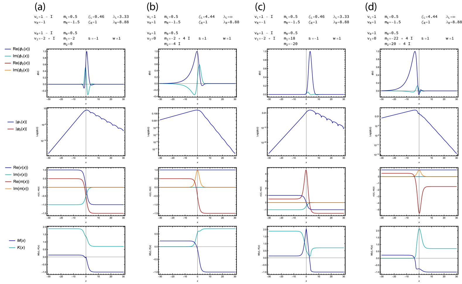
Figure 2: Zero modes on the interval $-\infty<x<\infty$ with a smooth domain wall given by S-shaped, symmetric or asymmetric Pöschl–Teller, or constant fields ${m}(x)$ and ${v}(x)$, and with its width smaller than or comparable with the characteristic decay lengths $w\lesssim\xi$. Panels on different rows from top to bottom show the spatial dependence of i) the real and imaginary parts of the wavefunctions, ii) the natural logarithm of the norm of the wavefunctions, iii) the real and imaginary parts of the fields ${m}(x)$ and ${v}(x)$, iv) the quantities ${M}(x)$ and ${K}(x)$. Panels on different columns from left to right correspond to different choices of the parameters ${m}_{0,1,2}$ and ${v}_{1,2}$, giving (a) single mode with exponentially damped oscillations on the right side and exponential decay on the left side of a smooth domain wall with an S-shaped field ${m}(x)$ and a complex S-shaped field ${v}(x)$ with $\mathrm{Im}({v}_{L})\neq 0$ (nonhermitian), (b) single mode with exponentially damped oscillations and nonuniform complex phase on the right side and exponential decay on the left side of a smooth domain wall with complex S-shaped field ${m}(x)$ with a nonzero imaginary component (nonhermitian). (c) single mode with exponentially damped oscillations and nonuniform complex phase on the right side and exponential decay on the left side of a smooth domain wall with asymmetric Pöschl–Teller field ${m}(x)$ and a complex S-shaped field ${v}(x)$ with $\mathrm{Im}({v}_{L})\neq 0$ (nonhermitian), (d) single mode with exponentially damped oscillations and nonuniform complex phase on the right side and exponential decay on the left side of a smooth domain wall with complex asymmetric Pöschl–Teller field ${m}(x)$ with a nonzero imaginary component (nonhermitian).

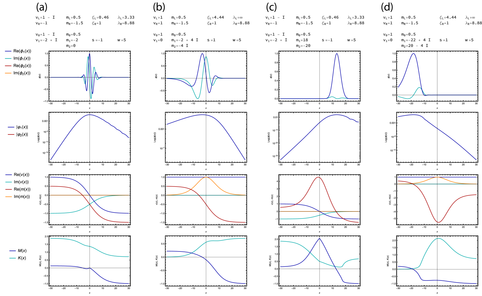
Figure 3: Zero modes on the interval $-\infty<x<\infty$ with S-shaped, symmetric, or asymmetric Pöschl–Teller, or constant fields ${m}(x)$ and ${v}(x)$ as in Fig.˜2, but where the width of the smooth domain wall is larger than the characteristic decay lengths $w>\xi$.

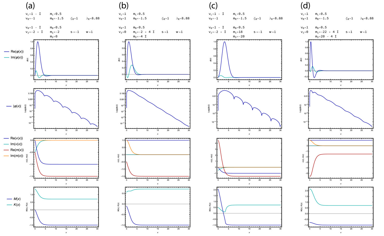
Figure 4: Zero modes on the interval $0\leq x<\infty$ with a smooth domain wall given by S-shaped, symmetric or asymmetric Pöschl–Teller, or constant fields ${m}(x)$ and ${v}(x)$, and with $w\lesssim\xi$. Panels on different rows are as in Fig.˜2. Panels on different columns from left to right correspond to different choices of the parameters ${m}_{0,1,2}$ and ${v}_{1,2}$ analogous to Fig.˜2, giving (a) single mode with exponentially damped oscillations with nonuniform complex phase on the right side of a smooth domain wall with S-shaped fields ${m}(x)$ and ${v}(x)$ with $\mathrm{Im}({v}_{R})\neq 0$ (nonhermitian), (b) single mode with exponentially damped oscillations with nonuniform complex phase on the right side of a smooth domain wall with S-shaped field ${m}(x)$ with a nonzero imaginary component (nonhermitian). (c) single mode with exponentially damped oscillations with nonuniform complex phase on the right side of a smooth domain wall with asymmetric Pöschl–Teller field ${m}(x)$ and S-shaped field ${v}(x)$ with $\mathrm{Im}({v}_{R})\neq 0$ (nonhermitian), (d) single mode with exponentially damped oscillations with nonuniform complex phase on the right side of a smooth domain wall with asymmetric Pöschl–Teller field ${m}(x)$ with a nonzero imaginary component (nonhermitian).

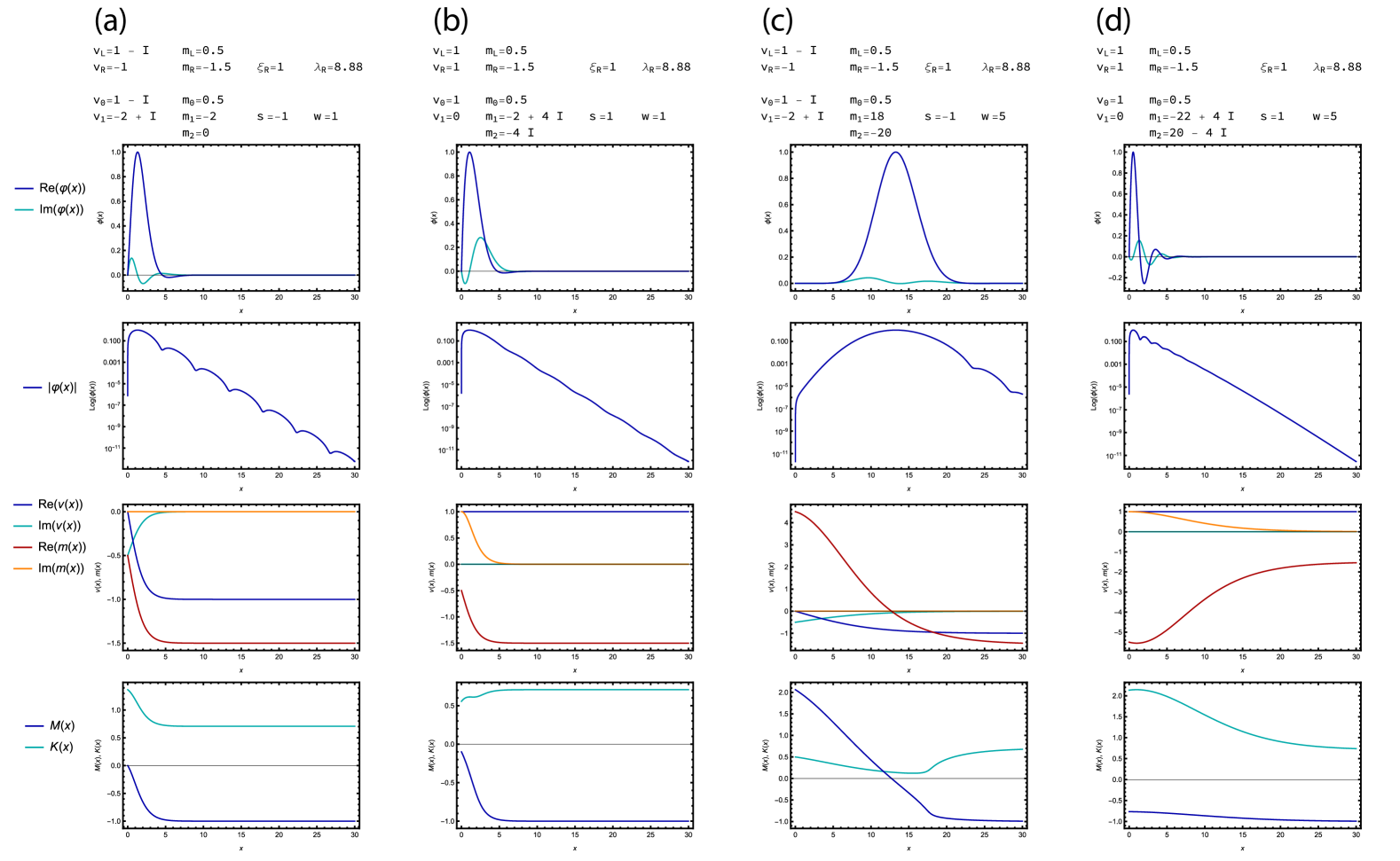
Figure 5: Zero modes on the interval $0\leq x<\infty$ with S-shaped, symmetric or asymmetric Pöschl–Teller, or constant fields ${m}(x)$ and ${v}(x)$ as in Fig.˜4, but with $w>\xi$.

IV.6 Experimental detection

From the definitions of the decay rates and momenta one has that $\mu_{L}^{\pm}+\mathrm{i}\kappa_{L}^{\pm}=-s{v}_{L}\pm\sqrt{{v}_{L}^{2}+{m}_{L}}$ and $\mu_{R}^{\pm}+\mathrm{i}\kappa_{R}^{\pm}=+s{v}_{R}\pm\sqrt{{v}_{R}^{2}+{m}_{R}}$, which yield

$$\mu_{L,R}+\mathrm{i}\kappa_{L,R}=\pm{v}_{L,R}\pm\sqrt{{v}_{L,R}^{2}+{m}_{L,R}},$$ (30)

which is valid for both hermitian and nonhermitian cases and both featureless and nonfeatureless zero modes. In the hermitian or in the asymptotically hermitian cases (i.e., if ${v}_{L,R},{m}_{L,R}\in\mathbb{R}$) and if the modes exhibit exponentially damped oscillations $\kappa_{L,R}\neq 0$, one gets $\mu_{L,R}=\pm{v}_{L,R}$ and consequently

$$\kappa_{L,R}^{2}+\mu_{L,R}^{2}=-{m}_{L,R},$$ (31)

which is valid for both featureless and nonfeatureless zero modes. Note that all the quantities on the left hand of Eqs.˜30 and 31 describe the wavefunction at large distances, in principle measurable by spatially-resolved spectroscopies, while the quantities on the right hand depend on the "bulk" properties of the system, i.e., the dispersion of bulk excitations of the system at large distances $x/w\to\pm\infty$. Thus, one can design an experiment in which some external parameters are varied and simultaneously measure the bulk dispersion at large distances and the decay rate and momenta of the zero modes. From these two sets of independent measures, one can thus obtain the quantities ${m}_{L,R}^{\text{exp}}$, ${v}_{L,R}^{\text{exp}}$ (bulk excitations) and $\mu_{L,R}^{\text{exp}}$, $\kappa_{L,R}^{\text{exp}}$ (zero modes). Strong evidence of the presence of zero modes is obtained when these quantities satisfy Eq.˜30 on an extended range of external parameters.

IV.7 Topological phases and differential order

We note that a general statement can be made on the maximum number of topologically protected modes and the maximum number of topologically distinct phases only by looking at the differential order of the Hamiltonian. The order of the differential equation determined by the Hamiltonian coincides with the maximum number of possible topologically protected modes and with twice the maximum possible value of the topological invariant as a consequence of the bulk-boundary correspondence. A second-order differential equation can support at most 2 linearly independent solutions satisfying the boundary conditions. Therefore, any Hamiltonian that can be reduced to a scalar second-order differential equation as in the modified Jackiw-Rebbi equation in Eq.˜3 may exhibit at most 2 topologically protected edge modes. In this case, the critical lines between topologically distinct phases, where the edge modes localize, can only separate phases with topological invariants $W,W^{\prime}$ with $|W-W^{\prime}|\leq 2$, due to the bulk-boundary correspondence. Hence, the topological invariant must be $|W|\leq 1$, with a maximum number of 2 nontrivial phases, regardless of the presence of antiunitary and unitary symmetries. More generally, given that an $n$-order differential equation can support at most $n$ linearly independent solutions satisfying the boundary conditions, any Hamiltonian that can be reduced to a scalar $n$-order differential equation may exhibit at most $n$ topologically-protected edge modes, and the critical lines can only separate distinct phases with topological invariants $W,W^{\prime}$ with $|W-W^{\prime}|\leq n$, which allows the presence of at most $\lfloor n/2\rfloor$ topologically nontrivial phases with $2|W|\leq n$, regardless of the presence of antiunitary and unitary symmetries.

V Conclusions

Concluding, we derived the analytical form of the wavefunctions of nonhermitian topological zero modes localized at smooth domain walls, by extending the modified Jackiw-Rebbi equation to nonhermitian systems with line gaps. Using these analytical results, we showed that the nonhermitian bulk-boundary correspondence for these systems can be directly derived by analyzing the asymptotic and localization properties of the zero modes. We thus identified a universal relation between the decay rates and oscillation wavelengths of the nonhermitian topological zero modes and the underlying scalar fields. This relation provides a direct link between the bulk properties and experimentally measurable physical quantities, which are, in principle, accessible via spatially resolved spectroscopies, suggesting an experimental way to probe nonhermitian topological zero modes. Analogously to their hermitian counterpart, the nonhermitian topological zero modes exhibit different localization behaviors, from featureless zero modes in the sharp domain wall limit to modes with "short" or "long hair" in the presence of smooth domain walls. Additionally, we showed that these modes can exhibit either pure exponential decay or exponentially damped oscillations in different regimes. These findings allow us to understand the physical properties of the zero modes, such as localization and oscillating behavior, that cannot be understood by topological considerations alone.

Appendix A Formal solutions of the modified Jackiw-Rebbi equation

We are specifically interested in the cases where the fields ${m}(x)$ and ${v}(x)$ are approximately uniform for $|x|>w$, and present nonnegligible spatial variations for $|x|<w$. This setup describes the case of a smooth domain wall between two uniform phases at $x\ll-w$ and $x\gg w$, or a sharp domain wall between two uniform phases at $x<0$ and $x>0$ in the limit $w\to 0$. In this setup, most of the interesting physics behavior is concentrated near the domain wall, and not at large distances. In this spirit, we map the whole real line $-\infty<x<\infty$ into the finite segment $0<y<1$ with the substitution

$$y(x)=\frac{1}{2}\left(1+\tanh{(x/2w)}\right)=\frac{{e}^{x/w}}{{e}^{x/w}+1},$$ (32)

where $w>0$ is a characteristic length describing the spatial variations of fields, i.e., the width of the smooth domain wall localized at the origin $x=0$. We thus expand the fields as a power series of $y$, with the assumption that the fields approach their asymptotic values on the left and right exponentially as

$$|{m}(x\to\mp\infty)-{m}_{L,R}|\sim{e}^{-|x|/w},$$ (33a)

$$|{v}(x\to\mp\infty)-{v}_{L,R}|\sim{e}^{-|x|/w}.$$ (33b)

Here, the characteristic length $w$ is, in principle, arbitrary but will be chosen, in practice, to match the characteristic length scale of the spatial variations of ${m}(x)$ and ${v}(x)$. The modified Jackiw-Rebbi equation in Eq.˜3 becomes

$$\varphi^{\prime\prime}(y)+\frac{1-2y+2ws{v}(y)}{y(1-y)}\varphi^{\prime}(y)-\frac{w^{2}{m}(y)}{y^{2}(1-y)^{2}}\varphi(y)=0,$$ (34)

which presents two regular singular points at $y=0,1$. Assuming a wavefunction in the form

$$\varphi(y)=y^{w\alpha_{L}}(1-y)^{w{\alpha_{R}}}F(y)$$ (35)

with $F(y)\neq 0$ at $y=0,1$, and expanding asymptotically at the singular points, we obtain the indicial equations for the exponents

$$\alpha_{L}^{2}+2s{{v}}_{L}{\alpha_{L}}-{m}_{L}=0,\qquad\alpha_{R}^{2}-2s{{v}}_{R}{\alpha_{R}}-{m}_{R}=0,$$ (36)

with solutions given by

$$\alpha_{L}^{\pm} =-s{{v}}_{L}\pm{q}_{L},\qquad{q}_{L}=\sqrt{{{v}}_{L}^{2}+{m}_{L}},$$ (37a)

$$\qquad\alpha_{R}^{\pm} =s{{v}}_{R}\pm{q}_{R},\quad\quad{q}_{R}=\sqrt{{{v}}_{R}^{2}+{m}_{R}}.$$ (37b)

For each set of exponents $({\alpha_{L}},{\alpha_{R}})=(\alpha_{L}^{\pm},\alpha_{R}^{\pm})$ the function $F(y)$ is given by the solution of the equation

$$F^{\prime\prime}(y)+\frac{C_{1}(y)}{y(1-y)}F^{\prime}(y)+\frac{C_{0}(y)}{y^{2}(1-y)^{2}}F(y)=0.$$ (38)

where

$$C_{1}(y)= {2w{\alpha_{L}}+1-2(w{\alpha_{L}}+w{\alpha_{R}}+1)y+2ws{v}(y)},$$ (39a)

$$C_{0}(y)= {w^{2}\alpha_{L}^{2}}-(2w{\alpha_{L}}+1)(w{\alpha_{L}}+w{\alpha_{R}})y$$

$$+(w{\alpha_{L}}+w{\alpha_{R}})(w{\alpha_{L}}+w{\alpha_{R}}+1)y^{2}-w^{2}{m}(y)$$

$$+2w\left(w{\alpha_{L}}-(w{\alpha_{L}}+w{\alpha_{R}})y\right)s{v}(y),$$ (39b)

are functions of $y$. There are four different choices of the exponents $(\alpha_{L}^{\pm},\alpha_{R}^{\pm})$, and for any of these choices, we obtain a distinct second-order differential equation for the function $F(y)$, which therefore admits two linearly independent solutions $F_{1,2}$. However, since the modified Jackiw-Rebbi is a differential equation is of second order, one can choose at most two solutions that are linearly independent: The general solution of the equation in Eq.˜3 is thus given by a linear combination of these two linearly independent solutions, e.g.,

$$\varphi_{1,2}^{s}(y)=y^{{w\alpha_{L}^{\pm}}}(1-y)^{{w\alpha_{R}^{\mp}}}F_{1,2}(y),$$ (40)

where $F_{1}(y)$ is one of the two solutions of Eq.˜38 corresponding to the exponents $(\alpha_{L}^{+},\alpha_{R}^{-})$ and $F_{2}(y)$ is one of the two solutions corresponding to the exponents $(\alpha_{L}^{-},\alpha_{R}^{+})$, chosen such that $\varphi_{1,2}^{s}(y)$ are linearly independent and well behaved at $y=0,1$, i.e., $\varphi_{1,2}^{s}(y\to 0)\sim y^{w\alpha_{L}^{\pm}}$ and $\varphi_{1,2}^{s}(y\to 1)\sim(1-y)^{w\alpha_{R}^{\mp}}$ in order to satisfy the boundary conditions. The last condition mandates that the functions converge in absolute value $|F(y)|<\infty$ for $y=0,1$ or, in the worst case, diverge logarithmically for $y\to 0$ or $y\to 1$. The solutions $F_{1,2}$ of Eq.˜38 can be determined by expanding the function $F(y)$ and the fields ${m}(y)$ and ${v}(y)$ in powers of $y$. We note again that the choice of the two linearly independent solutions in Eq.˜40 is not unique. Furthermore, choosing two linearly independent solutions is possible even if the exponents are degenerate, i.e., when $\alpha_{L,R}^{+}=\alpha_{L,R}^{-}$, as long as the functions $F_{1,2}$ are linearly independent.

Transforming back to the real line $-\infty<x<\infty$ the general solution is any linear combination

$$\varphi^{s}(x)=A_{1}\varphi_{1}^{s}(x)+A_{2}\varphi_{2}^{s}(x),$$ (41)

with $A_{1,2}\in\mathbb{C}$ and

$$\varphi_{1,2}^{s}(x)=G(\alpha_{L}^{\pm},\alpha_{R}^{\mp},x)F_{1,2}(x),$$ (42)

up to normalization constants with exponents given by Eq.˜37 and pseudospin in Eq.˜2 determined by the boundary conditions, where we define $G({\alpha_{L}},{\alpha_{R}},x)=y(x)^{w{\alpha_{L}}}(1-y(x))^{w{\alpha_{R}}}$ which is thus given by

$$G({\alpha_{L}},{\alpha_{R}},x)= \frac{{e}^{{\alpha_{L}\,x}}}{\left({e}^{{x}/{w}}+1\right)^{w{\alpha_{L}}+w{\alpha_{R}}}}$$

$$= \frac{{e}^{-{\alpha_{R}\,x}}}{\left({e}^{-{x}/{w}}+1\right)^{w{\alpha_{L}}+w{\alpha_{R}}}}$$

$$= \frac{{e}^{({\alpha_{L}}-{\alpha_{R}})x/2}}{\left(2\cosh{(x/2w)}\right)^{w{\alpha_{L}}+w{\alpha_{R}}}},$$ (43)

where we note that $G({\alpha_{L}},{\alpha_{R}},x)=G(-{\alpha_{L}},-{\alpha_{R}},x)^{-1}$, and with asymptotic behavior at large $x/w\to\pm\infty$ given by

$$G({\alpha_{L}},{\alpha_{R}},x\to\mp\infty)={{e}^{\mp{\alpha_{L,R}\,x}}}.$$ (44)

Moreover, if $0<|F_{1,2}|<\infty$, this also mandates that

$$\varphi_{1,2}^{s}(x\to-\infty) \sim{e}^{+\alpha_{L}^{\pm}\,x}={e}^{+\mu_{L}^{\pm}\,x}{e}^{+\mathrm{i}\kappa_{L}^{\pm}\,x},$$ (45a)

$$\varphi_{1,2}^{s}(x\to+\infty) \sim{e}^{-\alpha_{R}^{\mp}\,x}={e}^{-\mu_{R}^{\mp}\,x}{e}^{-\mathrm{i}\kappa_{R}^{\mp}\,x}.$$ (45b)

where $\mu_{L,R}^{\pm}=\mathrm{Re}(\alpha_{L,R}^{\pm})$ and $\kappa_{L,R}^{\pm}=\mathrm{Im}(\alpha_{L,R}^{\pm})$.

The asymptotic behavior of the functions $G({\alpha_{L}},{\alpha_{R}},x\to\pm\infty)$ does not depend on $w$ and on the functional form of the fields ${m}(x)$ and ${v}(x)$, but only on their values ${m}_{L,R}$ and ${v}_{L,R}$ at $x\to\pm\infty$. We will show that this property also holds for the solutions $\varphi_{1,2}^{s}(x)$ of the modified Jackiw-Rebbi equation in Eq.˜3.

Appendix B Exact solutions of the modified Jackiw-Rebbi equation

We found that the solutions $\varphi_{1,2}^{s}(x)$ can be written in closed form in terms of hypergeometric functions in the case where ${m}(y)$ and ${v}(y)$ can be expanded in powers of $y$, and these expansions can be truncated at the second order and first order, respectively, as

$${m}(x)= {m}_{0}+{m}_{1}y(x)+{m}_{2}y(x)^{2},$$ (46a)

$${v}(x)= {v}_{0}+{v}_{1}y(x),$$ (46b)

where ${m}_{0}={m}_{L}$, ${m}_{1}={m}_{R}-{m}_{L}-{m}_{2}$, ${m}_{2}=2({m}_{L}+{m}_{R})-4{m}(0)$, ${v}_{0}={v}_{L}$, and ${v}_{1}={v}_{R}-{v}_{L}$. At the zeroth order, Eq.˜46 describes the cases of constant fields ${m}(x)={m}_{L,R}={m}_{0}$ when ${m}_{1}={m}_{2}=0$ and ${v}(x)={v}_{L,R}={v}_{0}$ when ${v}_{1}=0$. At the first order, Eq.˜46 describes the case where the fields follow an S-shaped curve interpolating between ${v}_{L}={v}_{0}$ and ${v}_{R}={v}_{0}+{v}_{1}$ for $x=\pm\infty$, and interpolating between ${m}_{L}={m}_{0}$ and ${m}_{R}={m}_{0}+{m}_{1}$ when ${m}_{2}=0$. In particular, a symmetric S-shaped curve interpolating between ${v}_{L}={v}_{0}$ and ${v}_{R}=-{v}_{0}$ for $x=\pm\infty$ is obtained if ${v}_{1}=-2{v}_{0}$. At the second order, ${m}(x)$ in Eq.˜46 describes the symmetric Pöschl–Teller potential with ${m}_{L,R}={m}_{0}$ in the case where ${m}_{1}+{m}_{2}=0$ and an asymmetric Pöschl–Teller potential, i.e., a superposition of a Pöschl–Teller potential and an S-shaped potential otherwise.

If the expansion in Eq.˜46 holds, Eq.˜38 simplifies to

$$F^{\prime\prime}(y)+\frac{c-(a+b+1)y}{y(1-y)}F^{\prime}(y)-\frac{ab}{y(1-y)}F(y)=0,$$ (47)

which is the hypergeometric equation with $a,b,c$ depending on the exponents ${\alpha_{L}},{\alpha_{R}}$ as

$$a,b =w{\alpha_{L}}+w{\alpha_{R}}-ws{v}_{1}+\frac{1}{2}$$

$$\pm\frac{1}{2}\sqrt{\left(2ws{v}_{1}-1\right)^{2}+4w^{2}{m}_{2}},$$ (48a)

$$1-c =-2ws{v}_{L}-2w{\alpha_{L}},$$ (48b)

$$c-a-b =+2ws{v}_{R}-2w{\alpha_{R}}.$$ (48c)

The explicit expressions for $F_{1,2}$ in Eqs.˜42 and 40 are obtained by taking two solutions of the hypergeometric equation, i.e, choosing two linearly independent solutions out of the Kummer’s 24 solutions of the hypergeometric equation, which yields

$$f_{1}(y) ={{\,}_{2}F_{1}}\left(a,b,c,y\right),$$ (49a)

$$f_{2}(y) ={{\,}_{2}F_{1}}\left(a,b,a+b-c+1,1-y\right).$$ (49b)

Notice that, if one considers higher order terms in Eq.˜46, the resulting equation will not reduce to a hypergeometric equation in the general case. The equation above admits solutions that can be written in terms of two linearly independent solutions given by hypergeometric functions, although the choice is not unique. Hence, the explicit expressions for $F_{1,2}$ in Eq.˜40 are obtained by taking

$$F_{1}(y)= {{\,}_{2}F_{1}}(a_{1},b_{1},c_{1},y),$$ (50a)

$$F_{2}(y)= {{\,}_{2}F_{1}}(a_{2},b_{2},c_{2},1-y),$$ (50b)

where $a_{1},b_{1},c_{1}$ and $a_{2},b_{2},c_{2}$ are obtained from Eq.˜48 by substituting $({\alpha_{L}},{\alpha_{R}})=(\alpha_{L}^{+},\alpha_{R}^{-})$ and $({\alpha_{L}},{\alpha_{R}})=(\alpha_{L}^{-},\alpha_{R}^{+})$, respectively, giving

$$a_{1,2} =\pm w({{q}_{L}}-{{q}_{R}})$$

$$+\frac{1}{2}+\frac{1}{2}\sqrt{\left(2ws{v}_{1}-1\right)^{2}+4w^{2}{m}_{2}},$$ (51a)

$$b_{1,2} =\pm w({{q}_{L}}-{{q}_{R}})$$

$$+\frac{1}{2}-\frac{1}{2}\sqrt{\left(2ws{v}_{1}-1\right)^{2}+4w^{2}{m}_{2}},$$ (51b)

$$c_{1,2} =1+2{w{q}_{L,R}},$$ (51c)

provided that the corresponding solutions of the modified Jackiw-Rebbi equation in Eq.˜40 are linearly independent and can satisfy the boundary conditions. We notice that $a_{1}-a_{2}=b_{1}-b_{2}=c_{1}-c_{2}$ and that $b_{1,2}=1-a_{2,1}$.

Since ${q}_{L}$ and ${q}_{R}$ cannot be negative real numbers by definition, the hypergeometric functions above are well-defined, i.e., the hypergeometric function converges since $\mathrm{Re}(c_{1,2})\geq 1$ and therefore $c_{1,2}\notin\mathbb{Z}_{\leq}$. Moreover, to satisfy the boundary conditions, we must ensure that the functions defined above are sufficiently well-behaved at the extremes of the interval $0\leq y\leq 1$. We have that ${{\,}_{2}F_{1}}(a,b,c,0)=1$ which gives $F_{1}(0)=F_{2}(1)=1$. Furthermore, the asymptotic behavior of ${{\,}_{2}F_{1}}(a,b,c,y\to 1)$ depends on the value of $c-a-b$. Since, $c_{1}-a_{1}-b_{1}=c_{2}-1=2{w{q}_{R}}=2w\sqrt{{{v}}_{R}^{2}+{m}_{R}}$, by using the asymptotic properties of the hypergeometric functions, one obtains the following asymptotic behaviors, assuming $c_{1}-a_{1},c_{1}-b_{1}\notin\mathbb{Z}_{\leq}$. If either $a_{1}\in\mathbb{Z}_{\leq}$ or $b_{1}\in\mathbb{Z}_{\leq}$, the hypergeometric function reduces to a polynomial and one has

$${{\,}_{2}F_{1}}\left(a_{1},b_{1},c_{1},1\right)=\frac{\Gamma(c_{1})\Gamma(c_{1}-a_{1}-b_{1})}{\Gamma(c_{1}-b_{1})\Gamma(c_{1}-a_{1})}\neq 0,$$ (52)

which is nonzero since we assume $c_{1}-a_{1},c_{1}-b_{1}\notin\mathbb{Z}_{\leq}$. If $a_{1},b_{1},c_{1}-a_{1},c_{1}-b_{1}\notin\mathbb{Z}_{\leq}$, then $F_{1}(y)$ converges for $y\to 1$ to a nonzero value if $\mathrm{Re}({q}_{R})>0$ (e.g., ${{v}}_{R}^{2}+{m}_{R}>0$ in the asymptotically hermitian case ${v}_{R},{m}_{R}\in\mathbb{R}$) as

$$F_{1}(y\to 1)=\frac{\Gamma(c_{1})\Gamma(2w{q}_{R})}{\Gamma(c_{1}-a_{1})\Gamma(c_{1}-b_{1})}\neq 0,$$ (53)

it is bounded with oscillating behavior if $\mathrm{Re}({q}_{R})=0$ and ${q}_{R}\neq 0$ (e.g., ${{v}}_{R}^{2}+{m}_{R}<0$ in the asymptotically hermitian case ${v}_{R},{m}_{R}\in\mathbb{R}$) as

$$F_{1}(y\to 1) \sim(1-y)^{\mathrm{i}\mathrm{Im}(2w{q}_{R})}\frac{\Gamma(c_{1})\Gamma(-2w{q}_{R})}{\Gamma(a_{1})\Gamma(b_{1})}$$

$$+\frac{\Gamma(c_{1})\Gamma(2w{q}_{R})}{\Gamma(c_{1}-a_{1})\Gamma(c_{1}-b_{1})},$$ (54)

and it diverges logarithmically if ${q}_{R}=0$ (i.e., ${{v}}_{R}^{2}+{m}_{R}=0$) as

$$F_{1}(y\to 1)\sim-\frac{\Gamma(c_{1})}{\Gamma(a_{1})\Gamma(b_{1})}{\log\left(1-y\right)}.$$ (55)

Analogously, if $c_{2}-a_{2},c_{2}-b_{2}\notin\mathbb{Z}_{\leq}$ and either $a_{1}\in\mathbb{Z}_{\leq}$ or $b_{1}\in\mathbb{Z}_{\leq}$, then $F_{2}(0)$ is finite and nonzero, while if $a_{1},b_{1},c_{2}-a_{2},c_{2}-b_{2}\notin\mathbb{Z}_{\leq}$ then $F_{2}(y)$ converges for $y\to 0$ to a nonzero value if $\mathrm{Re}({q}_{L})>0$ (e.g., ${{v}}_{L}^{2}+{m}_{L}>0$ in the asymptotically hermitian case ${v}_{L},{m}_{L}\in\mathbb{R}$), it is bounded with oscillating behavior if $\mathrm{Re}({q}_{L})=0$ and ${q}_{L}\neq 0$ (e.g., ${{v}}_{L}^{2}+{m}_{L}<0$ in the asymptotically hermitian case ${v}_{L},{m}_{L}\in\mathbb{R}$), and it diverges logarithmically if ${q}_{L}=0$ (i.e., ${{v}}_{L}^{2}+{m}_{L}=0$) with asymptotic behavior given by analogous equations as in Eqs.˜52, 53, 54 and 55 where $a_{1},b_{1},c_{1}\to a_{2},b_{2},c_{2}$ and ${q}_{R}\to{q}_{L}$.

Hence, if $c_{1,2}-a_{1,2},c_{1,2}-b_{1,2}\notin\mathbb{Z}_{\leq}$, then $0<|F_{1,2}(y)|<\infty$ on the whole interval $0\leq y\leq 1$ or diverges logarithmically at the extremes of the interval. This ensures that $|\varphi_{1,2}^{s}(y\to 0)|\sim y^{w\mathrm{Re}(\alpha_{L}^{\pm}})$ and $|\varphi_{1,2}^{s}(y\to 1)|\sim(1-y)^{w\mathrm{Re}(\alpha_{R}^{\mp}})$. Finally, we notice that the choice of the functions $F_{1,2}$ in Eq.˜50 ensures that the solutions of the modified Jackiw-Rebbi equation in Eq.˜40 are linearly independent, since the Wronskian of the two solutions is

$$W\{\varphi_{1}^{s}\left(x\right),\varphi_{2}^{s}\left(x\right)\}=-\frac{\Gamma\left(c_{1}\right)\Gamma\left(c_{2}\right)}{\Gamma\left(c_{1}-a_{1}\right)\Gamma\left(c_{1}-b_{1}\right)}$$

$$\times y^{-sw{v}_{L}-1}(1-y)^{sw{v}_{R}-1}$$ (56)

which is always nonzero since we assume that $c_{1,2}-a_{1,2},c_{1,2}-b_{1,2}\notin\mathbb{Z}_{\leq}$.

Transforming back to the real line $-\infty<x<\infty$, the functions $F_{1,2}$ in Eq.˜42 are given by

$$F_{1,2}(x)={{{\,}_{2}F_{1}}\left(a_{1,2},b_{1,2},c_{1,2},\frac{1}{{e}^{\mp\,x/w}+1}\right)},$$ (57)

where we always assume that $c_{1,2}-a_{1,2},c_{1,2}-b_{1,2}\notin\mathbb{Z}_{\leq}$. Hereafter, for the sake of simplicity, we will not address explicitly the special cases where either $c_{1}-a_{1}=c_{2}-a_{2}\in\mathbb{Z}_{\leq}$ or $c_{1}-b_{1}=c_{2}-b_{2}\in\mathbb{Z}_{\leq}$, which may be obtained as limiting cases.

One has that $F_{1,2}(x\to\mp\infty)=1$. Furthermore, if $c_{1,2}-a_{1,2},c_{1,2}-b_{1,2}\notin\mathbb{Z}_{\leq}$, then $F_{1}(x)$ converges for $x\to\infty$ to a nonzero value if $\mathrm{Re}({q}_{R})>0$ (e.g., ${{v}}_{R}^{2}+{m}_{R}>0$ in the asymptotically hermitian case ${v}_{R},{m}_{R}\in\mathbb{R}$) while $F_{2}(x)$ converges for $x\to-\infty$ to a nonzero value if $\mathrm{Re}({q}_{L})>0$ (e.g., ${{v}}_{L}^{2}+{m}_{L}>0$ in the asymptotically hermitian case ${v}_{L},{m}_{L}\in\mathbb{R}$); $F_{1}(x)$ is bounded with oscillating behavior if $\mathrm{Re}({q}_{R})=0$ and ${q}_{R}\neq 0$ (e.g., ${{v}}_{R}^{2}+{m}_{R}<0$ in the asymptotically hermitian case ${v}_{R},{m}_{R}\in\mathbb{R}$) while $F_{2}(x)$ is bounded with oscillating behavior if $\mathrm{Re}({q}_{L})=0$ and ${q}_{L}\neq 0$ (e.g., ${{v}}_{L}^{2}+{m}_{L}<0$ in the asymptotically hermitian case ${v}_{L},{m}_{L}\in\mathbb{R}$); $F_{1}(x)$ diverges polynomially if ${q}_{R}=0$ (i.e., ${{v}}_{R}^{2}+{m}_{R}=0$) while $F_{2}(x)$ diverges polynomially if ${q}_{L}=0$ (i.e., ${{v}}_{L}^{2}+{m}_{L}=0$). These asymptotic behaviors are summarized in Table˜1. It follows that, if $c_{1,2}-a_{1,2},c_{1,2}-b_{1,2}\notin\mathbb{Z}_{\leq}$, then $0<|F_{1,2}(x)|<\infty$ on the whole real line or diverges polynomially for $x\to\pm\infty$.

As previously observed, in the hermitian case $\mathrm{Im}({m}(x))=\mathrm{Im}({v}(x))=0$, then the modified Jackiw-Rebbi equation in Eq.˜3 is real, and hence the solutions $\varphi_{1,2}^{s}(x)$ are either real or can be linearly combined into a set of linearly independent solutions which are real. In the nonhermitian case when $\mathrm{Im}({m}(x)\neq 0$ or $\mathrm{Im}({v}(x))\neq 0$ instead, the solutions $\varphi_{1,2}^{s}(x)$ cannot be linearly combined into a set of linearly independent solutions which are real.

In Table I of Ref. marra_topological_2024 are shown some special cases where the analytical expression of the general solution simplifies. In particular, we consider the cases where ${v}(x)={v}_{L,R}={v}$ is constant or a symmetric S-shaped curve (${v}_{0}={v}$ and ${v}_{1}=-2{v}$) with ${v}_{L,R}=\pm{v}$, and the cases where ${m}(x)={m}$ is constant or a symmetric Pöschl–Teller potential (${m}_{0}={m}$ and ${m}_{1}+{m}_{2}=0$), with ${m}_{L,R}={m}$, and more generally the case where ${q}_{L}={q}_{R}={q}$. In the cases considered, we have $|{v}_{L,R}|={v}$, and thus, we can assume ${v}\in\mathbb{R}$ up to a gauge transformation.

In particular, if ${q}_{L,R}={q}$, one has that $a_{1,2}=a$ and $b_{1,2}=b$ with $a+b=1$. In this case, the hypergeometric function can be written in terms of the associated Legendre functions as

$${{{\,}_{2}F_{1}}\left(a,b,c,\frac{1}{{e}^{\mp\,x/w}+1}\right)}=\Gamma(c){e}^{\pm{q}x}P^{1-c}_{-a}\left(\tanh\left(\mp\frac{x}{2w}\right)\right).$$ (58)

The correspondence between the hypergeometric functions and associated Legendre functions is the consequence of the fact that the hypergeometric equation can be transformed into a Legendre’s differential equation by mapping the interval $0\leq y\leq 1$ to the interval $-1\leq z\leq 1$ by the substitution $z=1-2y=\tanh(x/2w)$.

References

- (1) A. P. Schnyder, S. Ryu, A. Furusaki, and A. W. W. Ludwig, Classification of topological insulators and superconductors, AIP Conf. Proc. 1134, 10 (2009).
- (2) M. Hasan and C. Kane, Colloquium: Topological insulators, Rev. Mod. Phys. 82, 3045 (2010).
- (3) X.-L. Qi and S.-C. Zhang, Topological insulators and superconductors, Rev. Mod. Phys. 83, 1057 (2011).
- (4) S.-Q. Shen, W.-Y. Shan, and H.-Z. Lu, Topological insulator and the Dirac equation, SPIN 01, 33 (2011).
- (5) S.-Q. Shen, Topological insulators Dirac equation in condensed matters (Springer, 2017).
- (6) Y. Hatsugai, Chern number and edge states in the integer quantum Hall effect, Phys. Rev. Lett. 71, 3697 (1993).
- (7) S. Ryu and Y. Hatsugai, Topological origin of zero-energy edge states in particle-hole symmetric systems, Phys. Rev. Lett. 89, 077002 (2002).
- (8) J. Teo and C. Kane, Topological defects and gapless modes in insulators and superconductors, Phys. Rev. B 82, 115120 (2010).
- (9) Y. Ashida, Z. Gong, and M. U. and, Non-Hermitian physics, Adv. Phys. 69, 249 (2020).
- (10) N. Okuma and M. Sato, Non-Hermitian Topological Phenomena: A Review, Annu. Rev. Condens. Matter Phys. 14, 83 (2023).
- (11) H. Shen, B. Zhen, and L. Fu, Topological Band Theory for Non-Hermitian Hamiltonians, Phys. Rev. Lett. 120, 146402 (2018).
- (12) Z. Gong, Y. Ashida, K. Kawabata, K. Takasan, S. Higashikawa, and M. Ueda, Topological Phases of Non-Hermitian Systems, Phys. Rev. X 8, 031079 (2018).
- (13) K. Kawabata, K. Shiozaki, M. Ueda, and M. Sato, Symmetry and Topology in Non-Hermitian Physics, Phys. Rev. X 9, 041015 (2019).
- (14) F. Schindler, K. Gu, B. Lian, and K. Kawabata, Hermitian Bulk – Non-Hermitian Boundary Correspondence, PRX Quantum 4, 030315 (2023).
- (15) D. Nakamura, T. Bessho, and M. Sato, Bulk-Boundary Correspondence in Point-Gap Topological Phases, Phys. Rev. Lett. 132, 136401 (2024).
- (16) T. Gao, E. Estrecho, K. Y. Bliokh, T. C. H. Liew, M. D. Fraser, S. Brodbeck, M. Kamp, C. Schneider, S. Höfling, Y. Yamamoto, F. Nori, Y. S. Kivshar, A. G. Truscott, R. G. Dall, and E. A. Ostrovskaya, Observation of non-Hermitian degeneracies in a chaotic exciton-polariton billiard, Nature 526, 554 (2015).
- (17) A. Ghatak, M. Brandenbourger, J. van Wezel, and C. Coulais, Observation of non-Hermitian topology and its bulk–edge correspondence in an active mechanical metamaterial, Proceedings of the National Academy of Sciences 117, 29561 (2020).
- (18) W. Zhang, X. Ouyang, X. Huang, X. Wang, H. Zhang, Y. Yu, X. Chang, Y. Liu, D.-L. Deng, and L.-M. Duan, Observation of Non-Hermitian Topology with Nonunitary Dynamics of Solid-State Spins, Phys. Rev. Lett. 127, 090501 (2021).
- (19) R. Su, E. Estrecho, D. Biegańska, Y. Huang, M. Wurdack, M. Pieczarka, A. G. Truscott, T. C. H. Liew, E. A. Ostrovskaya, and Q. Xiong, Direct measurement of a non-Hermitian topological invariant in a hybrid light-matter system, Sci. Adv. 7, eabj8905 (2021).
- (20) C. Fleckenstein, A. Zorzato, D. Varjas, E. J. Bergholtz, J. H. Bardarson, and A. Tiwari, Non-Hermitian topology in monitored quantum circuits, Phys. Rev. Res. 4, L032026 (2022).
- (21) Q. Lin, T. Li, L. Xiao, K. Wang, W. Yi, and P. Xue, Observation of non-Hermitian topological Anderson insulator in quantum dynamics, Nat. Commun. 13, 3229 (2022).
- (22) B. Liu, Y. Li, B. Yang, X. Shen, Y. Yang, Z. H. Hang, and M. Ezawa, Experimental observation of non-Hermitian higher-order skin interface states in topological electric circuits, Phys. Rev. Res. 5, 043034 (2023).
- (23) A. Wang, Z. Meng, and C. Q. Chen, Non-Hermitian topology in static mechanical metamaterials, Sci. Adv. 9, eadf7299 (2023).
- (24) K. Ochkan, R. Chaturvedi, V. Könye, L. Veyrat, R. Giraud, D. Mailly, A. Cavanna, U. Gennser, E. M. Hankiewicz, B. Büchner, J. van den Brink, J. Dufouleur, and I. C. Fulga, Non-Hermitian topology in a multi-terminal quantum Hall device, Nat. Phys. 20, 395 (2024).
- (25) R. Jackiw and C. Rebbi, Solitons with fermion number, Phys. Rev. D 13, 3398 (1976).
- (26) P. Marra and A. Nigro, Topological zero modes and bounded modes at smooth domain walls: Exact solutions and dualities, Prog. Theor. Exp. Phys. 2025, 023A01 (2024).
- (27) P. Marra and A. Nigro, Zero Energy Modes with Gaussian, Exponential, or Polynomial Decay: Exact Solutions in Hermitian and non-Hermitian Regimes, Prog. Theor. Exp. Phys. 2025, 033A01 (2025).
- (28) A. Y. Kitaev, Unpaired Majorana fermions in quantum wires, Phys. Usp. 44, 131 (2001).