Computing Canonical Averages with Quantum and Classical Optimizers: Thermodynamic Reweighting for QUBO Models of Physical Systems

Abstract

Abstract. We present a general method to compute canonical averages for physical models sampled via quantum or classical quadratic unconstrained binary optimization (QUBO). First, we introduce a histogram reweighting scheme applicable to QUBO-based sampling constrained to specific intervals of an order parameter, e.g., physical energy. Next, we demonstrate that the scheme can accurately recover the density of states, which in turn allows for calculating expectation values in the conjugate ensemble, e.g., at a fixed temperature. The method can thus be used to advance the state-of-the-art characterization of physical systems that admit a QUBO-based representation and that are otherwise intractable with real-space sampling methods. A case in point are space-filling melts of lattice ring polymers, recently mapped in QUBO form, for which our method reveals that the ring catenation probability is non-monotonic with the bending rigidity.

Introduction The possibility of evaluating multiple solutions concurrently makes quantum computing ideally poised to solve optimization tasks in ways that are radically different from conventional methods. A prominent class of combinatorial problems solvable with quantum algorithms is quadratic unconstrained binary optimization (QUBO), which includes SAT, maximum clique, and graph coloring.

Solving a QUBO problem is equivalent to finding the ground state configuration(s) of a quadratic Ising-like Hamiltonian:

$$\mathcal{H}_{0}(\sigma)=\sum_{i}h_{i}\,\sigma_{i}\ +\sum_{i\neq j}J_{ij}\,\sigma_{i}\sigma_{j}\ ,$$ (1)

where the $h$ variables are the local external fields, $J$ is a symmetric interaction matrix, and the $\sigma$s are binary variables taking values of either 0 or 1.

In pursuit of potential advantages offered by quantum optimization and simulations Zhang et al. (2017); Albash and Lidar (2018); Kumar et al. (2020); Mazzola (2021); Layden et al. (2023); Abbas et al. (2023); Sandt and Spatschek (2023); Mazzola (2024); McArdle et al. (2020); Daley et al. (2022), and to leverage the practical speedups of special-purpose classical Ising machines Belletti et al. (2008a, b); Matsubara et al. (2018); Mohseni et al. (2022), researchers are increasingly recasting conventional sampling simulations of discrete physical systems as QUBO problems Perdomo-Ortiz et al. (2012); Lucas (2014); Hernandez and Aramon (2017); Xia et al. (2017); Li et al. (2018); Harris et al. (2018); King et al. (2018); Mulligan et al. (2019); Streif et al. (2019); Hauke et al. (2020); Willsch et al. (2020); Terry et al. (2020); Kitai et al. (2020); Carnevali et al. (2020); Micheletti et al. (2021); Hatakeyama-Sato et al. (2021); Yarkoni et al. (2022); Irbäck et al. (2022); Slongo et al. (2023); Baiardi et al. (2023); Irbäck et al. (2024). The mapping typically involves a one-to-one correspondence of the real-space configurations of the original system and the degenerate ground state solutions of an appropriate QUBO Hamiltonian. Uncorrelated configurations of the physical systems can thus be obtained by performing independent and unbiased minimizations of the QUBO Hamiltonian in the abstract space of its binary variables, followed by backmapping the solutions to real-space representations.

For soft matter systems, such as dense phases of polymers, resorting to the QUBO-based sampling on fully-quantum or hybrid classical-quantum annealers can be significantly more efficient than conventional Monte Carlo sampling in real space Slongo et al. (2023). Remarkably, the speedup benefits can be reaped, albeit to a lesser degree, even when the QUBO minimization is performed classically. A case in point is sampling maximally dense lattice ring polymers with infinite bending rigidity Slongo et al. (2023). Compared to real-space advanced sampling methods, numerical benchmarks show that classical QUBO-based sampling takes the runtime scaling with system size, $N$, from $N^{5.4}$ down to $N^{3.7}$.

QUBO-based sampling thus holds the promise of bringing significant performance improvements compared to Monte Carlo methods to many other instances of hard physical problems Perdomo-Ortiz et al. (2012); Lu and Li (2019); Robert et al. (2021); Irbäck et al. (2022); Ghamari et al. (2022); Linn et al. (2024), including protein design strategies and RNA secondary structure prediction Fox et al. (2022); Irbäck et al. (2024); Panizza et al. (2024). However, one known limitation is that QUBO-based sampling is natively tied to the microcanonical ensemble, unlike Monte Carlo methods, which naturally operate in the canonical ensemble. This is because QUBO schemes, as long as they are free of biases Moreno et al. (2003); Mandra et al. (2017), allow for covering the ground state manifold uniformly so that different energy-minimizing states are sampled with equal probability.

This limitation can be partly overcome in specific contexts, e.g., when excited states returned by quantum annealing runs are informative about the low-temperature Gibbs ensemble of the physical model Vuffray et al. (2022); Nelson et al. (2022); Ghamari et al. (2022); Sandt and Spatschek (2023); Layden et al. (2023). However, even aside from considerations of fair samplingMandra et al. (2017); Könz et al. (2019); Pochart et al. (2022), a general approach for calculating Boltzmann averages for QUBO representations of physical systems is still lacking.

In response to this challenge, here we introduce a QUBO-based scheme that enables computing canonical expectation values by combining the use of slack variables and a thermodynamic reweighting scheme. First, slack variables are introduced in the Hamiltonian to restrain the order parameter of interest, e.g., the energy of the physical model, within specific intervals. Next, a suitable weighted histogram method is used to combine data from overlapping intervals and thus recover the density of states. The latter is finally used to calculate expectation values in the conjugate ensemble, e.g., at a fixed temperature.

The approach is not restricted to computing energy-like expectation values and is, in principle, applicable to computing canonical averages of any order parameter. Accordingly, the method can be advantageously used on physical systems that are more tractable in QUBO form than in the native representation. For such systems, combining the intervalled QUBO-based sampling and reweighting scheme can significantly advance the characterization of the canonical equilibrium properties beyond state-of-the-art sampling methods such as real-space Monte Carlo.

We demonstrate this by considering space-filling melts of ring polymers. The system is, at one time, of broad interest in soft matter physics as well as a paradigm of the challenges of real-space sampling due to rapidly increasing autocorrelation times with system size and density. We show that our approach enables the first systematic characterization of inter-molecular linking of the rings as a function of their bending rigidity, revealing a non-monotonic relationship.

The findings highlight the method’s potential for providing breakthrough insights for QUBO-based physical models. They also motivate expanding the range of physical models mapped in QUBO form, where one could further harness the rapid development of optimization platforms using quantum algorithms and hardware.

I Multi-histogram reweighting for QUBO

I.1 Targeting QUBO-based sampling at energy intervals

We consider a QUBO-based encoding of a discrete physical system, represented by a Hamiltonian $\mathcal{H}$ whose ground states are in one-to-one correspondence with the admissible configurations of the physical system. As in eq. 1, $\mathcal{H}$ can include up to quadratic interactions of the variables $\sigma$, which take values 0 or 1. Throughout this manuscript, we interchangeably refer to the $\sigma$s as binary or spin variables, although in quantum computing contexts the latter term is commonly reserved for variables taking values $\pm 1$.

We further assume that the energy $E$ of the physical system – distinct from the QUBO Hamiltonian $\mathcal{H}$ – can be written as a linear combination of the spin variables with integer coefficients:

$$E=E_{0}+\Delta E\sum_{i}a_{i}\sigma_{i}$$ (2)

where the $a_{i}$s can also be null. Writing the physical energy in the form of eq. 2 may require introducing suitable ancilla spin variables Leib et al. (2016). Without loss of generality, in the following, we will set $E_{0}=0$ and $\Delta E=1$ unless otherwise stated. Specific examples for Ising and lattice polymer models will be discussed in Sections I.4 and II.

Plain QUBO-based sampling can be directed and restricted to single values of the discrete physical energy by complementing $\mathcal{H}_{0}$ of eq. 1 with a quadratic constraint that penalizes deviations of $E$ from $\bar{E}$:

$$\mathcal{H}\left(\sigma\right)=\mathcal{H}_{0}(\sigma)+A\left(\sum_{i}a_{i}\sigma_{i}-\bar{E}\right)^{2}\ ,$$ (3)

with $A>0$. Because the added constraint is quadratic, $\mathcal{H}$ is still a QUBO Hamiltonian. Its ground states manifold now provides a one-to-one coverage of the microcanonical ensemble at energy $\bar{E}$.

In principle, this energy targeting could be repeated for all admissible values of $\bar{E}$. However, even doing so would not enable the calculation of canonical averages since the necessary knowledge of the entropic weight of states at different energies can be gained only by targeting $E$ intervals spanning multiple energy levels rather than just a single value of $\bar{E}$.

To direct the QUBO-based sampling to a specific energy interval, we extend the space of spin variables to include a set of so-called slack variables, $s_{1},\ s_{2},...,\ s_{m}$. These variables are incorporated into a quadratic constraint that generalizes the one of eq. 3:

$$\mathcal{H}\left(\sigma\right)=\mathcal{H}_{0}(\sigma)+\left(\sum_{i}a_{i}\sigma_{i}-\bar{E}-\sum_{k=0}^{m-1}2^{k}s_{k}\right)^{2}\ .$$ (4)

Minimizing the above Hamiltonian enables the uniform sampling of microstates across the energy interval $E_{\rm min}\leq E\leq E_{\rm max}$, where $E_{\rm min}=\bar{E}$ and $E_{\rm max}=\bar{E}+\left(2^{m}-1\right)$. Systematically varying $\bar{E}$ allows for covering the energy spectrum of the physical system in its entirety.

I.2 Density of states from energy-intervalled sampling

The energy histograms obtained by sampling multiple overlapping energy intervals contain, in principle, sufficient information to reconstruct the density of states, $W(E)$, of the physical system. However, $W(E)$ cannot be reconstructed with standard weighted histogram analysis methods Ferrenberg and Swendsen (1989); Swendsen (1993); Tuckerman (2023). This is because weighted histogram methods are conceived for samples drawn from numerous Boltzmann or Boltzmann-like ensembles, a condition fundamentally different from our approach. In our framework, minimizing eq. 4 yields samples that lack Boltzmann-like statistical weights and, especially, are restricted to preassigned energy intervals of given widths and boundaries.

We use variational principles to derive a generalized weighted histogram analysis framework to recover $W(E)$ in this new context. This new method uses data sampled from multiple staggered energy intervals to optimally reconstruct $W(E)$ with gapless coverage of the energy range of interest.

We will use the following notation. The index $j$ labels the energy intervals, defined by $E_{\rm min}(j)\leq E\leq E_{\rm max}(j)$. The total number of microstates sampled for the $j$th interval is indicated by $N_{j}=\sum_{E}n_{j}(E)$, where $n_{j}(E)$ is the number of microstates with energy $E$ sampled for interval $j$.

The above quantities can be related to the density of states via:

$$\frac{\left\langle n_{j}(E)\right\rangle}{N_{j}}=\begin{cases}\frac{W(E)}{Z_{j}},&\text{if $E_{\rm min}(j)\leq E\leq E_{\rm max}(j)$}.\\ 0,&\text{otherwise}.\end{cases}$$ (5)

where the $\langle\rangle$ brackets denote the average over various realizations (sampling runs) and:

$$Z_{j}=\sum_{E_{\rm min}(j)\leq E\leq E_{\rm max}(j)}W(E)$$ (6)

Thus, by inverting the relationship of eq. 5 one has that the ratio $n_{j}(E)/{N_{j}}$ provides an estimator of $W(E)$ up to a multiplicative constant.

Note that an independent estimator for $W(E)$ can be obtained for each of the intervals covering the same energy level, $E$. These independent estimates can be combined into an optimal weighted average:

$$W(E)=\sum^{\prime}_{j}\alpha_{j}(E)\frac{n_{j}(E)}{N_{j}}\,Z_{j}\ ,$$ (7)

where the prime indicates that the sum is restricted to intervals that include $E$. For our purposes, the optimal $\alpha$s are those minimizing the error on the weighted sum. The variational calculation yields:

$$\alpha_{j}\propto\frac{1}{\delta n_{j}(E)^{2}}\cdot\frac{N_{j}^{2}}{\,Z_{j}^{2}}\ ,$$ (8)

and the proportionality coefficient is fixed by the constraint $\sum^{\prime}_{j}\alpha_{j}=1$.

Assuming that the microstates in each interval are sampled uniformly and using binomial statistics arguments, the variance of $n_{j}(E)$ can be written as:

$$\delta n_{j}(E)^{2}=g_{j}\langle n_{j}(E)\rangle\left(1-\frac{\langle n_{j}(E)\rangle}{N_{j}}\right)$$ (9)

where the factor $g_{j}=1+2\tau_{j}$ accounts for the possible finite autocorrelation time, $\tau_{j}$, of the microstate sampling process Müller-Krumbhaar and Binder (1973). When samples are uncorrelated, e.g. when obtained from independent quantum annealing runs, then $g_{j}=1$.

Combining expressions of eqs. 5, 8 and 9 yields:

$$W(E)=\frac{\sum_{j}^{\prime}\frac{n_{j}(E)}{g_{j}\left(1-\frac{W(E)}{Z_{j}}\right)}}{\sum_{k}^{\prime}\frac{N_{k}}{Z_{k}g_{k}\left(1-\frac{W(E)}{Z_{k}}\right)}}\ .$$ (10)

Note that the density of states can be reconstructed only up to a multiplicative constant, which can be set by imposing the normalization condition:

$$\sum_{E}W(E)=1\ .$$ (11)

The sought $W$s in the desired energy range are obtained by treating eq. 10 as a set of self-consistent equations to be solved iteratively. The procedure, its algorithmic formulation and convergence are presented in Supporting Information Section S1.

From the reconstructed $W(E)$ profile, the canonical expectation value of a generic observable, ${\cal O}$, at temperature $T$ can be obtained via thermodynamic reweighting Vernizzi et al. (2020); Tuckerman (2023):

$$\langle{\cal O}\rangle_{T}=\frac{\sum_{E}\langle{\cal O}\rangle_{E}\,\,W(E)e^{-\beta E}}{\sum_{E}W(E)e^{-\beta E}}$$ (12)

where $\beta=(k_{B}\,T)^{-1}$ and $\langle{\cal O}\rangle_{E}$ and $\langle{\cal O}\rangle_{T}$ are the averages of ${\cal O}$ at fixed energy $E$ and temperature $T$, respectively. Again, the mentioned summand-sorting procedure may be necessary for numerical precision.

We note that, though the optimally weighted averaging of eq. 8 is inspired by conventional histogram reweighting methods Ferrenberg and Swendsen (1989); Swendsen (1993); Tuckerman (2023), the two reconstruction approaches are fundamentally different. In the conventional case, recovering the density of states requires undoing the Boltzmann weight of overlapping histograms, collected at different temperatures, covering the energy range of interest. The position and width of the histograms cannot be enforced a priori because they are system- and temperature-dependent and hence need to be chosen through tentative or pre-conditioning runs. Instead, in our scheme, the sampling can be expressly directed at user-defined energy intervals of desired width position, thus facilitating the coverage of the energy range of interest.

I.3 Error analysis

To estimate the errors of the reconstructed $W(E)$, we resort to a block-like analysis that makes it straightforward to account for the correlations between the $n_{j}$s, $Z$s, and $W$s. For simplicity, we assume that all addressed energy intervals are covered with the same ”sampling depth,” $N_{j}=N$, and that the sampled states are uncorrelated ($\tau_{j}=0)$. For each interval, we subdivide the samples into $s$ blocks of equal size, $N/s$. Next, we carry out $s$ reconstructions of the density of states, using for each interval the first block, then the second, and so on, obtaining a total of $s$ independent (normalized) profiles, $W_{1}(E),W_{2}(E),\dots,W_{s}(E)$. The final $W$ profile and its statistical uncertainty are obtained by computing the mean of the $W_{i=1,\dots,s}$ and the associated statistical error for each value of $E$.

I.4 Validation

To validate the QUBO-based reconstruction of $W(E)$, we applied it to an exactly solvable physical system. To this end, we considered the Ising model on the $L\times L$ square lattice with uniform nearest-neighbour spin interactions and periodic boundary conditions. For even $L$, the density of states can be calculated exactly with the recursive enumeration method of ref.  Beale (1996). Because the energy of the system is solely determined by the number of parallel neighboring spins, $2n_{\shortparallel}$, we used $n_{\shortparallel}$ as the natural variable for profiling $W$, and mapped the admissible configurations on the QUBO model detailed in Appendix A.

The admissible range of $n_{\shortparallel}$ is bound by 0 and $L^{2}$, corresponding respectively to the antiferromagnetic and ferromagnetic states. $W(n_{\shortparallel})$ is unimodal and symmetric with respect to the midpoint $n_{\shortparallel}=L^{2}/2$. $W$ is minimum at the boundaries, where the ferromagnetic and antiferromagnetic states account for two configurations each, and is maximum at the midpoint.

For a stringent validation, we considered the $12\times 12$ Ising system ($L=12$), where the ”dynamic range” of $W$ spans across more than 40 orders of magnitude, making it impossible to recover the entire profile of $W(n_{\shortparallel})$ with simple sampling schemes. For the reconstruction, we used $m=1$, $2$, and $3$ slack variables, corresponding to $n_{\shortparallel}$ intervals of width $2$, $4$, and $8$, respectively, and sampled the ground state manifold using a parallel tempering scheme (see Supporting Information S2). We leveraged the unbiassed nature of classical parallel tempering-based optimizations to decouple the validation of the reconstruction method from potential external biases. These include those that can arise from, e.g. fair-sampling issues in quantum optimizersMandra et al. (2017); Könz et al. (2019); Pochart et al. (2022),and out-of-equilibrium effects in classical annealersMoreno et al. (2003).

As illustrated in Appendix A, the reconstructed profiles are practically indistinguishable from the exact one at all $m$s, and the observed agreement is remarkably consistent throughout the broad range spanned by $W$, despite its wide dynamic range. Furthermore, the reported data demonstrate that the block analysis provides a reliable and unbiased estimate of the statistical uncertainty of the reconstructed $W$.

II Application: Adding bending rigidity to ring polymer melts

We now apply the approach to characterize the topological entanglement in equilibrated melts of semiflexible, topologically unrestricted ring polymers. The canonical sampling of such a system is challenging for conventional approaches based on real-space representations, such as molecular dynamics or Monte Carlo simulations. Consequently, no results are available for how knotting and linking probabilities change with the rings’ bending rigidity.

These questions are relevant across diverse contexts, from biology and physical chemistry to material science and soft matter physics. For instance, polymer ring melts are key reference systems for understanding the unique features of the multiscale genome organization Grosberg et al. (1993); Rosa and Everaers (2014); Abdulla et al. (2023), and how topoisomerase enzymes influence it Piskadlo et al. (2017); Roca et al. (2022). Additionally, modern interpretations of density-induced phase transitions in liquids are related to entanglements of closed paths along the chemical bonds of the system Neophytou et al. (2022, 2024). Dense systems of circular molecules are also crucial for prospective realization of topological meta-materials, including Olympic gels and self-assembled molecular chainmails Luengo-Márquez et al. (2024); Klotz et al. (2020); Polles et al. (2016); Chiarantoni and Micheletti (2023); Liu et al. (2022); Gil-Ram´ırez et al. (2015); Rauscher et al. (2020a, b). Finally, in soft matter contexts, melts of rings polymers are at the heart of ongoing endeavors to understand anomalous relaxation dynamics and response to shear flow Ito (2007), aging of active topological glasses Smrek et al. (2020), and how it is affected by both chain density and topology O’Connor et al. (2020); Smrek et al. (2020); Farimani et al. (2024); Micheletti et al. (2024).

The computational challenges in tackling these systems arise from their high packing densitySchmid (2022). The latter dramatically hinders the physical relaxation of the chains, making it computationally prohibitive to obtain uncorrelated equilibrated samples using molecular dynamics simulations. An analogous slowing down affects Monte Carlo simulations, too. By employing non-local (non-physical) moves, Monte Carlo methods can often speed up the sampling compared to molecular dynamics. However, the acceptance rate of such non-local moves drops significantly with increasing system density, again due to steric clashes. The problem is exacerbated when going from fully flexible to semi-rigid and finally to rigid rings. These challenges affect continuum and lattice polymer models alike.

II.1 QUBO-based reconstruction of the density of states

Prompted by these considerations, we addressed the entanglement of canonically equilibrated self-assembled melts of lattice ring polymers for arbitrary values of their bending rigidity $\kappa_{b}$. We adopted the QUBO-based formulation of lattice polymers introduced in refs.  Micheletti et al. (2021); Slongo et al. (2023), which enables the sampling of self-assembled ring melts on regular and irregular lattices, and considered the stringent case of ring melts that fill cubic lattices of $N$ sites.

As detailed in Appendix B, the QUBO Hamiltonian for such systems can be formulated in terms of two types of Ising-like binary variables attached respectively to individual lattice edges and pairs of incident edges meeting at $\pi/2$ angles. The two sets of variables are introduced to keep track of (i) the lattice edges that are occupied by the bonds of the self-assembled rings and (ii) the number of corner turns of the rings, $n_{c}$.

Note that on hypercubic lattices, as in the considered case, $n_{c}$ is proportional to the total curvature of the ring melt up to a $\pi/2$ factor. It is thus the parameter of choice for the density of states, $W(n_{c})$, required to compute the desired canonical expectation values as a function of the conjugate variable, i.e. the ring’s bending rigidity, $\kappa_{b}$.

We reconstructed $W(n_{c})$ for space-filling ring melts on a $5\times 5\times 4$ cubic lattice for a total of 100 lattice sites; see (b-h) panels in Fig. 2. To cover the entire admissible range $32\leq n_{c}\leq 100$, we used multiple intervalled samplings with unit increment in $\bar{n}_{c}$ and $m=3$ slack variables, corresponding to intervals of widths 8. Considering the numerous intervals involved, we performed the sampling with a parallel tempering scheme on a classical high-performance computing cluster, and reserved the use of quantum optimization platforms to the more manageable $3\times 3\times 2$ system, which we discuss later.

The density of states obtained using $m=3$ variables is shown in Fig.1.

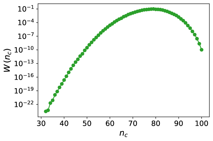
Figure 1: Density of states as a function of total curvature for a ring melt filling a $5\times 5\times 4$ lattice. The reconstruction was obtained using a sampling depth $d\approx 1,000$ for each of the $69$ intervals of length $8$ ($m=3$) straddling

the entire range of curvature values, $32\leq n_{c}\leq 100$. The data points represent the average density of states computed from $4$ reconstructions; error bars are smaller than the symbol size, because the average error is around $5\%$.

$W\left(n_{c}\right)$ is peaked around $n_{c}=78$, which would be the most probable value of $n_{c}$ for curvature-unrestricted sampling. $W$ decreases rapidly on both sides of the peak, dropping by more than 9 and 22 orders of magnitude to the right and left, respectively.

We note that if the same total number of states were collected from a curvature-unrestricted QUBO sampling, rather than from multiple overlapping intervals, then the single resulting histogram would only cover the $60\leq n_{c}\leq 96$ range. This limited coverage would preclude the calculation of the entire $W$ profile and, hence, of canonical expectation values at arbitrary $\beta\kappa_{b}$.

II.2 Canonical expectation values for varying bending rigidity

The density of states $W(n_{c})$ enables calculating the expectation values of a generic observable, $\mathcal{O}$, at fixed inverse temperature, $\beta$, and bending rigidity, $\kappa_{b}$, via:

$$\langle\mathcal{O}\rangle_{\beta\kappa_{b}}=\frac{\sum_{n_{c}}\langle\mathcal{O}\rangle_{n_{c}}W\left(n_{c}\right)e^{-\beta\kappa_{b}n_{c}}}{\sum_{n_{c}}W\left(n_{c}\right)e^{-\beta\kappa_{b}n_{c}}}\ ,$$ (13)

where $\langle\mathcal{O}\rangle_{n_{c}}$ is the average of the observable of interest computed at fixed $n_{c}$. In the above expression, which specializes eq. 12 to self-assembled ring melts, we have set $E=\kappa_{b}n_{c}$, thereby absorbing the curvature of $\pi/2$ at each corner turn into the definition of $\kappa_{b}$.

Note that $W$ is the same for any considered observable and, therefore, needs to be reconstructed only once by covering the admissible range of $n_{c}$ with overlapping intervals. In addition, it is advantageous to compute the constrained average, $\langle\mathcal{O}\rangle_{n_{c}}$, using (uncorrelated) states with the given $n_{c}$ from all intervals that include $n_{c}$.

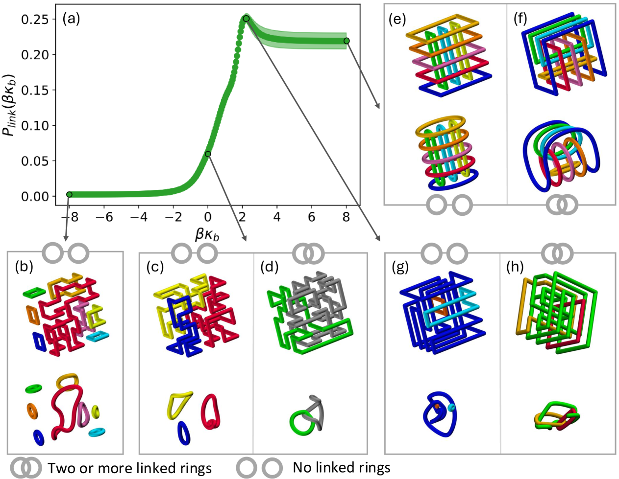
Figure 2: Equilibrium linking probability of melts of self-assembled rings as a function of the reduced bending rigidity $\beta\kappa_{b}$. (a) Linking probability $P_{\rm link}$ for a canonically-equilibrated ring melt filling a $5\times 5\times 4$ cubic lattice. The data points represent the average $P_{\rm link}$ computed from $4$ reconstructions and the shaded bands indicate the standard error of the mean. The considered range of $\beta\kappa_{b}$ spans from -8 to +8, i.e. from strongly favoured to strongly suppressed corner turns. Across this range, the linking probability is non-monotonic, peaking at $\beta\kappa_{b}\sim 2$. Panels (b-h) show typical configurations at the values of $\beta\kappa_{b}$ indicated by the callouts. The configurations were randomly picked among those with $n_{c}$ equal to the average curvature at the corresponding value $\beta\kappa_{b}$.

II.3 Results: linking probability

We used the above scheme to profile the linking (concatenation) probability of canonically equilibrated melts of rings as a function of the bending rigidity.

Concatenation constraints, also termed mechanical bonds, are key structural motifs for supramolecular self-assemblies, from self-limited synthetic catenanes Chichak et al. (2004); Beves et al. (2011); Polles et al. (2016); Marenda et al. (2018) to modular ones Niu and Gibson (2009); Wu et al. (2017); Datta et al. (2020); Chiarantoni and Micheletti (2022, 2023), including three-dimensional Olympic gels Speed et al. (2024).

In recent years, various experimental advancements Yamamoto and Tezuka (2015); Yamamoto et al. (2016), especially in metal-ion templating techniques, have finally made it possible not only to externally control the geometry and topology of mechanical bonding but also to boost the yield of these topological constructs. However, despite these breakthroughs, identifying the conditions most conducive to inter-molecular linking remains an open problem.

In this regard, the bending rigidity, $\kappa_{b}$ is a natural parameter for the design of topologically-bonded materials. However, studying the effect of $\kappa_{b}$ on concatenation probability of long and densely packed rings is challenging for real-space Monte Carlo and molecular dynamics because the autocorrelation times increase rapidly with the rings’ rigidity. For instance, high effective bending rigidities, e.g., due to electrostatic repulsions, can cause the dynamical arrest in ring melts Staňo et al. (2023); in addition, concatenation constraints significantly slow down the system’s relaxation dynamics Datta and Virnau (2024). Consequently, profiling inter-chain linking in canonical equilibrium has so far been feasible only for a few distinct values of $\beta\kappa_{b}$ and for discrete models amenable to special-purpose sampling methods Ubertini and Rosa (2023). Thus, how mutual entanglements in ring melts vary as a function of $\beta\kappa_{b}$ remains an unsolved problem for conventional Monte Carlo methods. For the same reasons, it is the natural avenue for applying the QUBO-based sampling and the thermodynamic reweighting technique. In fact, our recent study of ref. Slongo et al. (2023) has shown the potential of using QUBO-based models to profile the entanglement of ring melts. However, such considerations were restricted to the microcanonical constant-curvature ensemble, preventing to draw any conclusion for the conjugate canonical ones as a function of $\beta\kappa_{b}$.

Accordingly, we computed the $\beta\kappa_{b}$ dependence of the linking probability, $P_{\rm link}$, defined as the probability that self-assembled states contain at least one linked pair of rings. To this end, we used eq. 13 after identifying $\langle\mathcal{O}\rangle_{n_{c}}$ in with $P_{\rm link}(n_{c})$.

The resulting $P_{\rm link}(\beta\kappa_{b})$ is shown in Fig. 2a. The shaded band denotes the estimated statistical error on the average. Notice that $\beta\kappa_{b}$ is varied continuously and that positive and negative values of the bending rigidity can be seamlessly considered. The negative bending rigidity case, corresponding to situations where bending is energetically favored, is addressed rarely in conventional simulations.

The data in Fig. 2b establishes a remarkable novel result, namely that the linking probability has a unimodal dependence on $\beta\kappa_{b}$.

The non-monotonic dependence of the linking probability on bending rigidity is best discussed considering the limiting cases where $\beta\,\kappa_{b}$ takes on large negative and positive values.

For $\beta\kappa_{b}<-4$, $n_{c}$ is maximum, corresponding to a $\pi/2$ turn at each lattice site. The resulting rings are so tightly wound that they do not leave openings that can be threaded by the other rings thereby preventing linking. In the opposite case, $\beta\kappa_{b}>4$, typical configurations correspond to nested stacked rings – similar to the columnar structures observed in concentrated solutions of semiflexible ring polymers Poier et al. (2016) – as illustrated Fig. 2e. The rings in these columnar structures are planar and, hence, free of intra-chain entanglement (knotting). However, their inter-chain entanglement (linking) remains possible in the form of interlocked ring stacks, as shown in Fig. 2f. Consequently, $P_{\rm link}$ attains a finite value for $\beta\kappa_{b}\gg 0$. Remarkably, the two limits are bridged non-monotonically, with the maximum linking probability occurring at $\beta\kappa_{b}\sim 2$.

We conclude that a finite bending rigidity is required to balance two opposite effects: on the one hand, rings must not be too flexible or meandering because some degree of directional persistence is necessary to form loops wide enough to be threadable. On the other hand, while a large stiffness does produce configurations that could be threadable, it also suppresses configurational entropy, and hence it is not optimally conducive to linking.

The generality and robustness of the nonmonotonicity of $P_{\rm link}(\beta\kappa_{b})$ is indicated by the fact that it does not depend on whether the number of self-assembled rings is allowed to fluctuate or is set equal to 3 or more rings by a posteriori selection, see Appendix B and Fig. S1.

This behavior has not been previously reported or observed in polymer systems at large. The result significantly advanced the understanding of how bending rigidity influences the topological entanglement of polymer systems. Previous studies have been limited to single, isolated polymers, where the only possible form of topological entanglement is intra-chain (i.e., knotting), which is also unimodal with respect to bending rigidity Coronel et al. (2017). Interestingly, we found an analogous knotting property for rings that are not isolated but are part of self-assembled melts, as shown in Appendix B. The shared unimodality of both linking and knotting probabilities reveals a previously unrecognized connection and common microscopic basis between the intra- and inter-ring entanglements in spite of their otherwise very distinct nature.

We expect that the unimodality of $P_{\rm link}$, here established for a maximally dense system of ring melts, ought to manifest more broadly, e.g., at partial space-filling and in various realizations of supramolecular self-assemblies or topologically-unrestricted ring polymers. The applicative potential of the result to boost the inherently low yield of molecular interlockings in supramolecular self-assemblies Gil-Ram´ırez et al. (2015); Polles et al. (2016). Our results indicate that a judicious design of the bending rigidity of the circular elements could afford considerable latitude for tuning and maximizing the concatenation probability. For instance, in the case of Olympic gels assembled from individually circularizable linear DNAs Speed et al. (2024), two such control parameters would be the ionic strength/valency of the solution and the DNA length, which can influence the effective rigidity by modulating the DNA persistence length and the number of Kuhn lengths, respectively.

III Application to Quantum Annealers

Compared to conventional sampling methods, such as Monte Carlo of molecular dynamics with real-space polymer representations, the QUBO formulation can offer significant speedups with both classical and quantum optimizers. This advantage was demonstrated in ref. Slongo et al. (2023), which examined the computational cost of sampling space-filling ring melts with minimum curvature as a function of the system size (total ring length), $N$. For ad hoc optimized real-space sampling, the computational cost scaled as $N^{5.4}$, while QUBO-based sampling improved the scaling to $N^{3.7}$ with classical annealers and to $N^{3.2}$ with hybrid classical-quantum ones.

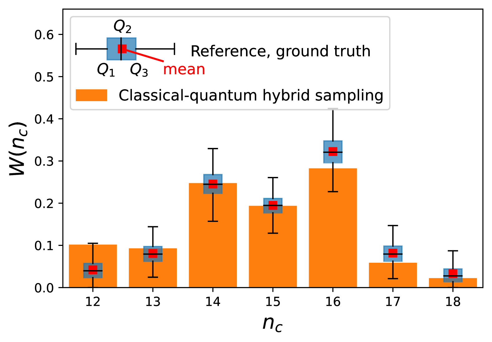
Figure 3: Validation of the density of states reconstructed from classical-quantum hybrid sampling of a ring melt filling a $3\times 3\times 2$ lattice. The reconstruction (orange histograms) was computed from samples obtained with the D-wave hybrid sampler, using a sampling depth $d=50$ for each of the $4$ intervals of length $4$ ($m=2$) spanning the entire range of curvature values, $12\leq n_{c}\leq 18$. The ground truth normalized density of states was obtained by exhaustive enumeration of all possible states. The box plots represent the probability distribution of $500$ independent reconstructions obtained via unbiased sampling of the exhaustively enumerated set, using the same intervals and depth $d$ as with the hybrid sampler. $Q1$, $Q2$ and $Q3$ mark the first, second (median), and third quartiles, respectively. The whiskers extend to the furthest data points within 1.5 IQR of the box edges, where IQR is the interquartile range ($Q_{1}$ to $Q_{3}$).

The implications are twofold. On the one hand, QUBO-based sampling of soft matter can already be advantageous on classical machines, for which computing power is widely available. On the other hand, as the size and power of quantum machines continue to advance, integrating quantum annealers and QUBO-based models could become a relevant and performative tool for physical systems where real-space MC schemes are hindered by the rapid growth of autocorrelation times with system size.

Towards these prospective applications, we used the D-Wave implementation of quantum annealers to assess their potential for reconstructing the density of states without biases arising from fair-sampling issues Mandra et al. (2017); Könz et al. (2019); Pochart et al. (2022).

For such proof of concept demonstration, we considered ring melts in a $3\times 3\times 2$ cuboid. This system size was chosen because it is sufficiently large to feature hundreds of distinct states across a certain curvature range, $12\leq n_{c}\leq 18$. At the same time, the entire conformational ensemble can be explored with exhaustive enumeration methods, which we leveraged to establish the exact density of states and the statistical confidence intervals of its reconstructions at a given sampling depth.

For the reconstruction, we used $m=2$ slack variables to cover the above-mentioned $n_{c}$ range with $4$ staggered intervals of 4 bins each. We set the sampling depth of each interval to 50, thus maintaining coverage well below the exhaustive limit. The minimization of the QUBO Hamiltonians, which involved $115$ qubits, was performed with the D-Wave hybrid classical-quantum sampler with the default runtime of 3s. Although this was the minimum runtime allowed, it consistently yielded one of the ground states at each minimization trial.

The density of states reconstructed from the hybrid sampling is presented in Fig. 3 alongside the ground truth result, i.e., the statistical distribution of equivalent reconstructions based on the uniform sampling of the exhaustively enumerated states. The comparison shows that the reconstruction based on the hybrid classical-quantum sampling is fully consistent with the ground truth reference. For instance, about half of the data points (4 out of 7 bins) fall within the Q1-Q3 interquartile range.

The result provides a proof-of-concept demonstration of the feasibility of using quantum optimization platforms for intervalled sampling that are sufficiently uniform that accurate reconstructions of the density of states can be achieved. With the constant improvements of quantum platforms, our method could thus enable studying QUBO-mapped physical models with significant speed improvements over classical optimizers.

IV Conclusions

We have introduced a general method to compute expectation values of observables by reweighting microstates obtained by minimizing QUBO Hamiltonians of physical models.

QUBO models are natively suited to sample systems with fixed order parameters, e.g. microstates at a fixed energy of the physical model, since their values can be straightforwardly fixed with quadratic constraints in the QUBO Hamiltonian. Our method enables computing observables in the conjugate ensembles, e.g. canonical averages at fixed temperature. First, we turn the quadratic constraints of the order parameters into quadratic restraints by introducing slack variables. In this way, the QUBO-based sampling can be directed towards finite intervals of the constrained order parameter. Next, we target an overlapping series of intervals that cover the entire range of interest of the order parameter. The gathered states are then processed with a generalized histogram reweighting technique to optimally reconstruct the density of states, which is finally harnessed to compute the sought expectation values in the conjugate ensembles.

The general formulation of our method makes it usable with different conjugate ensembles, as we demonstrated by using the method in two different contexts.

First, we validated the approach for the 2D Ising model, for which the density of states is known exactly. Using a $12\times 12$ system, we demonstrated that the method enables a bias-free reconstruction of the entire density of states. By using multiple energy intervals, and sampling negligible fraction of the entire configuration space, we achieved an average relative reconstruction accuracy of order $10^{-2}$ across the 42 orders of magnitudes spanned by the density of states.

Finally, we explored the topological entanglement of a melt of self-assembled semiflexible rings, which is relevant across diverse contexts, from polymer physics to synthetic supramolecular constructs and designed metamaterials. The problem is challenging for conventional sampling methods using real-space representations, and no results have heretofore been established for ring melts about how intra- and inter-ring entanglement vary with the bending rigidity. By leveraging the available efficient mapping to QUBO models and applying our reweighting method to states sampled in multiple intervals of the bending energy, we obtained the knotting and linking probabilities for a broad range of bending rigidities, the conjugate order parameter. We thus established, among other results, that the linking probability is non-monotonic and can be maximized at a suitable value of the bending rigidity. The result establishes, for the first time, that the linking probability in systems of topologically unrestricted ring polymers has a non-monotonic dependence on bending rigidity. Besides advancing the characterization of dense polymer self-assemblies beyond state-of-the-art real-space sampling methods, the findings suggest new ways to optimize mechanical-bonding in extended supramolecular assemblies, such as Olympic gels.

In both these contexts, the uniform sampling of the ground state manifold of the QUBO Hamiltonians was performed using a parallel tempering scheme on a classical computer. However, quantum optimization platforms are the ideal avenue for our method because they can afford increasing practical speedups as their size and performance continues to improve. To this end, we used classical-quantum optimizers to sample exhaustively-enumerable ring melts, and demonstrated the feasibility of obtaining accurate reconstructions of the density-of-states for computing canonical averages.

Our scheme can be extended in several directions, both for formulation and applications. For instance, the method can be generalized to reconstruct the density of states that are functions of several order parameters, $W(\mu_{1},\mu_{2},...)$. This would involve equipping the QUBO Hamiltonian with a quadratic restraint for each parameter and generalizing the self-consistent equations for $W$. In addition, while the powers-of-two linear combination of slack variables provides a natural uniform coverage of the intervals, it may be more efficient to devise other combination schemes designed to counteract the entropic suppression arising from wide dynamic ranges of the density of states. In this case, the self-consistent equations for $W$ would need to be adjusted to take into account the sampling biases introduced ad hoc. By the same token, data from the intervalled QUBO sampling could be combined with that from unconstrained sampling, performed with QUBO or even conventional methods.

Prospective applications of our method include QUBO-mapped physical systems that call for being treated in the canonical ensemble. For instance, incorporating finite-temperature considerations could enhance the realism of models in soft matter and biological physics, including protein folding, protein design, and RNA secondary structure predictions, which have all been mapped to QUBO models.

V Acknowledgments

We are grateful to Pietro Faccioli, Philipp Hauke, and Guglielmo Mazzola for feedback on the manuscript. We thank CINECA for access to the D-Wave platform under the PRACE programme. This study was funded in part by the European Union - NextGenerationEU, in the framework of the PRIN Project ”The Physics of Chromosome Folding” (code: 2022R8YXMR, CUP: G53D23000820006) and by PNRR Mission 4, Component 2, Investment 1.4_CN_00000013_CN-HPC: National Centre for HPC, Big Data and Quantum Computing - spoke 7 (CUP: G93C22000600001). The views and opinions expressed are solely those of the authors and do not necessarily reflect those of the European Union, nor can the European Union be held responsible for them.

Appendix A: Density of states reconstruction for the $L\times L$ Ising system

QUBO model for the $L\times L$ Ising system

To perform the QUBO-based reconstruction of $W$ for the 2D Ising system, we introduce the following QUBO-Hamiltonian, which involves site ($\sigma_{i}$) and edge ($\eta_{ij}$, $\theta_{ij}$) variables on the $L\times L$ lattice, as well as slack variables ($s_{k}$):

$$\mathcal{H}=\mathcal{H}_{0}+A\mathcal{H}_{s}=\sum_{\langle ij\rangle}V_{ij}+A\mathcal{H}_{s}\ ,$$ (14)

where:

$$V_{ij} =\left(1+2\sigma_{i}\sigma_{j}+2(\sigma_{i}+\sigma_{j})\eta_{ij}\right.$$

$$\left.-4(\sigma_{i}+\sigma_{j}+\eta_{ij})\theta_{ij}-\sigma_{i}-\sigma_{j}-\eta_{ij}+8\theta_{ij}\right)$$ (15)

$$\mathcal{H}_{s} =\left(\sum_{\langle ij\rangle}\eta_{ij}-2\bar{n}_{\shortparallel}-2\sum_{k=0}^{m-1}2^{k}s_{k}\right)^{2}\ .$$ (16)

In the above expressions, $A$ is a non-negative coefficient, which we set equal to 1, and $\sum_{\langle ij\rangle}$ indicates the summation over distinct pairs of neighboring lattice sites.

The $\sigma_{i}={0,1}$ binary site variables are in one-to-one correspondence with the up/down spins of the physical Ising model. The $\eta$ binary variables are instead introduced to keep track of parallel and antiparallel neighboring spins. They are tied to the $\sigma$s by an XNOR relation, which is enforced as a quadratic QUBO constraint involving the binary ancilla variables, $\theta$. This is best seen by setting $A=0$, which reduces the QUBO Hamiltonian to ${\cal H}_{0}$. In this case, minimizing the Hamiltonian for a given spin configuration $\sigma$ amounts to minimizing the individual quadratic terms $V_{ij}$, yielding the sought XNOR relation:

$$\eta_{ij}=\begin{cases}1&\text{if }\sigma_{i}=\sigma_{j},\\ 0&\text{otherwise.}\end{cases}$$ (17)

We note that the expressions for $V_{ij}$ are constructed such that for any set of the $\sigma$ variables – each mappable to a unique set of physical spins – the energy-minimizing $\eta$s and $\theta$s yield ${\cal H}_{0}=0$. Thus, the degenerate ground states of ${\cal H}_{0}$ are in one-to-one correspondence with the possible spin configurations and, thanks to the ancilla $\theta$ variables, also with the associated $\eta$s, which represent the parallel or antiparallel alignment of neighboring spins.

A schematic representation of the $\sigma$ and $\eta$ variables of a ground state solution of ${\cal H}_{0}$ in a $4\times 4$ system is shown in Fig. 4.

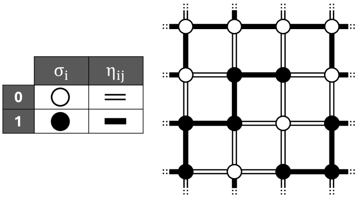
Figure 4: Example of QUBO encoding for energy-constrained Ising models. Left: Symbolic representation of QUBO binary variables associated to up/down physical spins ($\sigma_{i}$) and parallel/antiparallel spin pairs ($\eta_{ij}$). Right: The represented state is one of the possible ground state solutions of the QUBO Hamiltonian of eq. 14 formulated for a $4\times 4$ periodic Ising system with ${\cal H}_{s}$ parameters set to $\bar{n}_{\shortparallel}=8$ and $m=0$. The ground state solutions correspond to Ising spin configurations with $16$ pairs of parallel neighbouring spins, including those wrapping across the periodic boundary conditions (dotted).

The second quadratic term in eq. 14, which involves slack variables, has the same structure as that of eq. 4. Its minimization ensures that the number of parallel spins, $2n_{\shortparallel}=\sum_{\langle ij\rangle}\eta_{ij}$, falls within the interval $[2\bar{n}_{\shortparallel},2\bar{n}_{\shortparallel}+2^{m+1}-2]$.

Thus, by minimizing the total Hamiltonian of Eq. 14 the sampling can be targeted at specific intervals of $n_{\shortparallel}$, as needed for reconstructing the density of states $W(n_{\shortparallel})$.

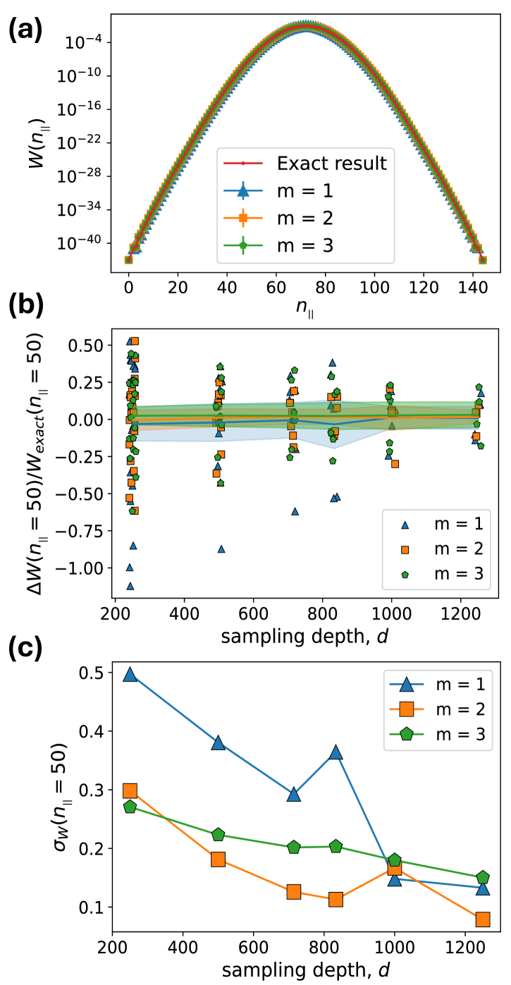
Figure 5: Density of states of the $12\times 12$ Ising model. (a) Exact and reconstructed density of states, $W(n_{\shortparallel})$ for a $12\times 12$ Ising model as a function of the number of parallel neighbouring spins. The data in this and the following panels are color-coded according to the number of slack variables and distinguished by different marker shapes. (b) Normalized reconstruction error, $\Delta W(n_{\shortparallel}=50)/W_{\rm exact}(n_{\shortparallel}=50)$, for different sampling depths, $d$. The solid lines connect the average values of $\Delta W(n_{\shortparallel}=50)$ computed from independent reconstructions. The data points include jitter along the $x$-axis for visual clarity. Non-overlapping blocks of $d$ samples were used from a population of 5000 independent samples per interval. The shaded bands indicate the standard error of the mean. (c) Statistical error of the reconstructed density of states, $W$, as a function of sampling depth, $d$, for $n_{\shortparallel}=50$.

Comparison of exact and reconstructed $W$s

We considered the $12\times 12$ Ising system ($L=12$) with periodic boundary conditions. The argument $n_{\shortparallel}$ can take on $L^{2}-1$ distinct values, corresponding to all integers between $0$ and $144$, except for $1$ and $L^{2}-1=143$. The peak value of $W$ is $\sim 2\times 10^{42}$, thus indicating that the ”dynamic range” of the density of states spans across more than 40 orders of magnitude.

For the QUBO-based reconstruction, we used multiple intervalled samplings with unit increments in $\bar{n}_{\shortparallel}$. We considered intervals of width $2$, $4$, and $8$, corresponding to $m=1$, $2$ and $3$ slack variables, respectively.

We covered each of the $\sim 150$ intervals with a sampling depth of $d\sim 5,000$ independent states. The latter were obtained using a classical parallel tempering scheme to minimize the QUBO Hamiltonian (Supporting Information Section S2).

The reconstructed $W$s are compared with the normalized exact one Beale (1996) in the semi-log plot of Fig. 5a, which shows a remarkably consistent agreement throughout the 40 orders of magnitude spanned by $W$.

The reconstructed profiles are visually indistinguishable from the exact one at all $m$s, although there are differences. While $W(n_{\shortparallel})$ can be accurately reconstructed across the entire range of the argument using $m=2$ and $m=3$, this is not the case for $m=1$, where $W$ is not resolved close to boundaries $n_{\shortparallel}=0$ and $n_{\shortparallel}=L^{2}$. This is because $m=1$ intervals are too short to bridge the gaps at $n_{\shortparallel}=1,L^{2}-1$.

At the same time, longer and longer intervals are not necessarily beneficial, as they would cover broader dynamic ranges of $W$, thus increasing the sampling depth $d$ required to cover the entire interval. Thus, the optimal choice of $m$ should be made by taking into account the variation of $W$ and the gaps of its argument.

To quantitatively assess the effect of sampling depth $d$ on reconstruction fidelity, we divided the $5,000$ collected states for each interval into $s$ non-overlapping blocks, each comprising $d$ microstates, with $d$ ranging from $200$ to $1250$. Next, we obtained $s$ independent reconstructions, $W_{1}$, $W_{2}$, … , $W_{s}$, by using respectively only the data from the first block of each interval, then from the second block, etc.

We next considered the pointwise error of the profiles:

$$\Delta W_{i}(n_{\shortparallel})=W_{i}(n_{\shortparallel})-W_{\rm exact}(n_{\shortparallel})\ ,$$ (18)

and computed the mean and variance of these errors across the $s$ equivalent and independent reconstructions:

$$\langle\Delta W(n_{\shortparallel})\rangle =\langle W(n_{\shortparallel})\rangle-W_{\rm exact}(n)$$

$${\rm Var}\left[\Delta W(n_{\shortparallel})\right] =\langle\Delta W^{2}(n_{\shortparallel})\rangle-\langle\Delta W(n_{\shortparallel})\rangle^{2}$$ (19)

$$={\rm Var}\left[W(n_{\shortparallel})\right]$$

where $\langle.\rangle$ denotes the average over the $s$ block estimates.

Fig. 5b shows the results of the error analysis for the representative bin $n_{\shortparallel}=50$, corresponding to one of the two midpoints of $\log(W)$. For clarity, the data are normalized to the exact $W$ value, $W_{\rm exact}(n_{\shortparallel}=50)$. For all considered $m$s, we observe that the $\Delta W_{i}$ values (data points) are clustered around zero. In fact, their means (solid lines) are compatible with zero within the estimated error on the mean (shaded band), which is equal to:

$${\rm Var}\left[\langle\Delta W(n_{\shortparallel})\rangle\right]=\frac{{\rm Var}\left[\Delta W(n_{\shortparallel})\right]}{\sqrt{s-1}}$$ (20)

Note that the results also establish that $\langle W\rangle$ is compatible with $W_{\rm exact}$ within the estimated error. Considering that the latter can be calculated without reference $W_{\rm exact}$ (see eq. Comparison of exact and reconstructed $W$s), we conclude that multiple independent reconstructions of the normalized $W$ allow for computing the associated statistical uncertainty in a reliable and unbiased manner.

In addition, the third panel shows the error on the individual reconstructions, $\sqrt{{\rm Var}\left[\Delta W(n_{\shortparallel})\right]}$, which decreases with the sampling depth for all $m$s.

Appendix B: melt of self-assembled rings with varying bending rigidity

QUBO-based sampling of self-assembled ring melts

We consider ring melts that completely fill cubic lattices of $N$ index sites. A QUBO Hamiltonian for such systems can be formulated in terms of two types of Ising-like binary variables, hereafter indicated as $\Gamma^{-}$ and $\Gamma^{\llcorner}$. A $\Gamma^{-}_{ij}$ variable is attached to each lattice edge, $ij$, to indicate whether a bond is present (1, active) or absent (0, inactive) between neighboring sites $i$ and $j>i$. Similarly, a $\Gamma^{\llcorner}_{ijk}$ variable is assigned to each corner triplet of sites, $j$ being neighbor to both $i$ and $k>i$. This variable indicates whether the two incident edges $ij$ and $jk$ are both occupied by bonds (1, active) or not (0, inactive).

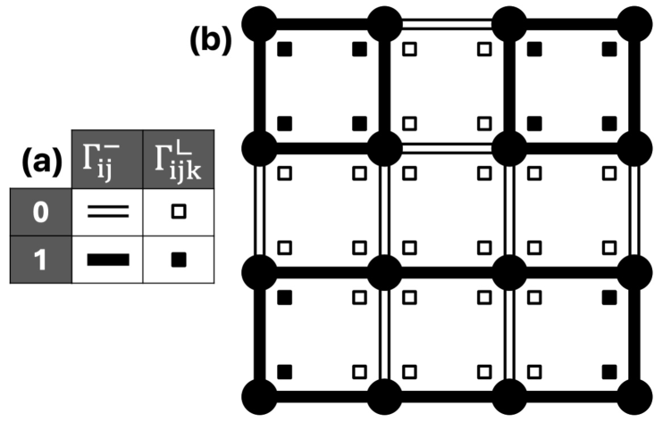
Figure 6: Example of QUBO encoding for space-filling melts of ring polymers. (a) Symbolic representation of QUBO binary variables corresponding to occupied/empty bonds ($\Gamma_{ij}^{-}$) and corner triplets ($\Gamma_{ijk}^{\llcorner}$). (b) The represented configuration is one of the possible ground state solutions of the QUBO Hamiltonian of eq. 21 formulated for a $4\times 4$ square lattice and with the setting $N=16$ to impose space-filling. In this example, the total curvature (number of corner turn) is $n_{c}=12$.

Using the above variables, the QUBO Hamiltonian for the system reads Slongo et al. (2023):

$${\cal H}_{N}=A_{\textrm{b}}\left({\sum}_{\langle ij\rangle}\Gamma^{-}_{ij}-N\right)^{2}+A_{\textrm{c}}{\sum}_{\langle ijk\rangle}{\sum}^{\prime}_{\langle ljm\rangle}\Gamma^{\llcorner}_{ijk}\Gamma^{\llcorner}_{ljm}$$

$$+A_{\textrm{bc}}{\sum}_{\langle ijk\rangle}\left[3\Gamma^{\llcorner}_{ijk}+\Gamma^{-}_{ij}\Gamma^{-}_{jk}-2\Gamma^{\llcorner}_{ijk}(\Gamma^{-}_{ij}+\Gamma^{-}_{jk})\right]$$ (21)

where the $A$ coefficients are non-negative, $\sum_{\langle ij\rangle}$ and $\sum_{\langle ijl\rangle}$ indicate summations over distinct neighboring pairs and triplets of lattice sites, respectively. The prime indicates the restriction over inequivalent triplets, $\langle ijk\rangle\neq\langle ljm\rangle$.

The first quadratic term is minimized when the total number of bonds (active edges) is equal to the number of lattice sites $N$, as required by the space-filling condition of the ring melt. The second term is a quadratic constraint that enforces the consistency of the $\Gamma^{-}$ and $\Gamma^{\llcorner}$ variables. In fact, this term is minimized if and only if the active corners of $\Gamma^{\llcorner}$ are compatible with the active bonds of $\Gamma^{-}$, i.e.,

$$\Gamma^{\llcorner}_{ijk}=\begin{cases}1,&\text{if }\Gamma^{-}_{ij}=\Gamma^{-}_{jk}=1\\ 0,&\text{otherwise.}\end{cases}$$ (22)

Finally, the third quadratic term is minimized when no branching is present and thus penalizes cases where three or more bonds meet at the same lattice site. Combining this constraint with the first one, i.e., that the number of active bonds is equal to the number of sites, implies that each site has exactly two incident bonds and is, therefore, part of a closed chain.

Thus, minimizing all three terms simultaneously yields a binary encoding of self-assembled polymers that satisfy the physical requirements of being space-filling, self-avoiding, and exclusively consisting of closed chains. Notice that the number of closed chains is not fixed and is determined by the self-assembly combinatorics.

The ground states of the QUBO Hamiltonian of eq. 21, which by construction correspond to ${\cal H}_{N}=0$, are thus in one-to-one correspondence with the configurations of maximally-dense melts of rings.

A schematic representation of the $\Gamma^{-}$ and $\Gamma^{\llcorner}$ of a ground state solution of ${\cal H}_{N}$ is shown in Fig. 6. For clarity, the illustrated case is for a two-dimensional $4\times 4$ lattice.

QUBO-based sampling for a bending energy interval

As noted in connection with eq. 13, a natural parameter for profiling the density of states $W$ is the total number of corner turns, $n_{c}$. This quantity is proportional to the total curvature and, hence, is the conjugate variable of the bending rigidity. In the ground state manifold ${\cal H}_{N}$, $n_{c}$ can be directly computed from the number of active $\Gamma^{\llcorner}$ variables in the ground states of ${\cal H}_{N}$:

$$n_{c}=\sum_{\langle ijk\rangle}\Gamma^{\llcorner}_{ijk}\ .$$ (23)

The intervalled sampling required to reconstruct $W(n_{c})$ can thus be achieved by adding to ${\cal H}_{N}$ a quadratic term proportional to:

$${\cal H}_{s}=\left(\sum_{\langle ijk\rangle}\Gamma^{\llcorner}_{ijk}-\bar{n}_{c}-\sum_{k=1}^{m}2^{k}\right)^{2}\ .$$ (24)

In fact, minimizing ${\cal H}_{N}+A{\cal H}_{s}$ with $A>0$ allows for sampling states in the interval $\bar{n}_{c}\leq n_{c}\leq\bar{n}_{c}+2^{m-1}$.

Repeating the sampling procedure for overlapping intervals covering the entire range of $n_{c}$, and applying the reconstruction method of section 1, one can obtain the full profile of the density of states $W()$.

Ring melt composition versus bending rigidity

The composition of the self-assembled rings melts is conveniently characterized in terms of the average number of self-assembled rings at fixed temperature and bending rigidity, $\langle N_{\rm rings}\rangle_{\beta\kappa_{b}}$. We recall that the number of chains in self-assembling polymer systems can be controlled with extrinsic design parameters, such as monomer density, and intrinsic ones, such as the monomers’ bonding volume Sciortino (2016). In our case, the former is fixed by the space-filling conditions, while the latter is varied via the bending rigidity.

We computed $\langle N_{\rm rings}\rangle_{\beta\kappa_{b}}$ using eq. 13 after identifying $\langle\mathcal{O}\rangle_{n_{c}}$ with the average number of rings per each admissible value of $n_{c}$, $\langle N_{\rm rings}\rangle_{n_{c}}$.

Fig. 7 illustrates the resulting profile of $\langle N_{\rm rings}\rangle_{\beta\kappa_{b}}$, obtained by averaging five independent reconstructions. The shaded band denotes the estimated statistical error on the average profile, which is typically smaller than $0.6$% except for $\beta\kappa_{b}<4$.

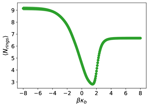
Figure 7: Average number of self-assembled rings as a function of the reduced bending rigidity $\beta\kappa_{b}$. The results are for a canonically equilibrated ring melt filling a $5\times 5\times 4$ cubic lattice. The data points represent the average $P_{\rm link}$ computed from $4$ reconstructions and the shaded bands indicate the standard error of the mean. The considered range of $\beta\kappa_{b}$ spans from $-8$ to $+8$, i.e. from strongly favoured to strongly suppressed corner turns. Across this range, the average number of rings is non-monotonic, having a minimum at $\beta\kappa_{b}\sim 1.5$.

For $\beta\kappa_{b}>4$, $\langle N_{\rm rings}\rangle_{\beta\kappa_{b}\gg 0}$ plateaus at about $6.5$. In this regime of large bending rigidity, typical configurations of the ring melt correspond to nested stacked rings, which typically involves approximately $7$ rings on $5\times 5\times 4$ space-filled lattice, as illustrated in Fig. 2e.

For $\beta\kappa_{b}<-4$, instead, $\langle N_{\rm rings}\rangle$ plateaus to about 9. This larger asymptotic value reflects the fact that, when chain turns are favored, the rings are smaller and hence more numerous, as shown in Fig. 2b.

Fig. 7 shows that in between two asymptotic values $\langle N_{\rm rings}\rangle_{\beta\kappa_{b}}$ is minimum for $\beta\kappa_{b}\sim 1.7$, where it is slightly smaller than 3. A typical configuration for such extremal case is shown in Fig. 2g-h.

Knotting probability versus bending rigidity

To characterize the intra-ring entanglement, we considered the knotting probability, defined as the probability that individual rings in the melt are knotted, $P_{\rm knot}$. To compute the knotting dependence on $\beta\kappa_{b}$, we used eq. 13 after identifying $\langle O\rangle_{n_{c}}$ in with $P_{\rm knot}\left(n_{c}\right)$.

The resulting $P_{\rm knot}$ vs $\beta\kappa_{b}$ curve is shown in Fig. 8. The curve approaches zero for large $\beta|\kappa_{b}|$, irrespective of the sign of the bending rigidity.

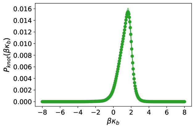
Figure 8: Equilibrium knotting probability of melts of self-assembled rings as a function of the reduced bending rigidity $\beta\kappa_{b}$. Knotting probability $P_{knot}$ for a canonically-equilibrated ring melt filling a $5\times 5\times 4$ cubic lattice. The data points represent the average $P_{knot}$ computed from $4$ reconstructions. The associated errors, indicated by the shaded band, are typically smaller than the symbol size, except near the peak. The considered range of $\beta\kappa_{b}$ spans from $-8$ to $+8$, i.e. from strongly favoured to strongly suppressed corner turns. Across this range, the knotting probability is non-monotonic, peaking at $\beta\kappa_{b}\sim 1.6$.

In the limit $\beta\kappa_{b}>4$, the vanishing knotting probability is due to the mentioned nested columnar structures. Since the stacked rings are planar, they are necessarily unknotted, too. Instead, in the opposite situation ($\beta\kappa_{b}<-4$), the microscopic basis for the vanishing $P_{\rm knot}$ is fundamentally different. In this regime, $n_{c}$ is largest, corresponding to a $\pi/2$ turn at each lattice site. These tightly wound rings do not leave openings that can be threaded by the other parts of the chain, thereby preventing knot formation (see Fig. 2b).

Between these two limits, $P_{\rm knot}$ is maximum for $\beta\kappa_{b}\sim 2$. In this regard, we recall that various systems of isolated rings have been shown to have a non-monotonic knotting probability as a function of bending rigidity, from lattice polymer models Orlandini et al. (2005), to off-lattice open Virnau et al. (2013) and closed chains Coronel et al. (2017). Our results demonstrate that this result, previously established only for isolated chains, equally applies to polymer melts, too.

References

- Zhang et al. (2017) B. H. Zhang, G. Wagenbreth, V. Martin-Mayor, and I. Hen, Scientific reports 7, 1044 (2017).
- Albash and Lidar (2018) T. Albash and D. A. Lidar, Physical Review X 8, 031016 (2018).
- Kumar et al. (2020) V. Kumar, C. Tomlin, C. Nehrkorn, D. O’Malley, and J. Dulny III, arXiv preprint arXiv:2007.08487 (2020).
- Mazzola (2021) G. Mazzola, Physical Review A 104, 022431 (2021).
- Layden et al. (2023) D. Layden, G. Mazzola, R. V. Mishmash, M. Motta, P. Wocjan, J.-S. Kim, and S. Sheldon, Nature 619, 282 (2023).
- Abbas et al. (2023) A. Abbas, A. Ambainis, B. Augustino, A. Bärtschi, H. Buhrman, C. Coffrin, G. Cortiana, V. Dunjko, D. J. Egger, B. G. Elmegreen, et al., arXiv preprint arXiv:2312.02279 (2023).
- Sandt and Spatschek (2023) R. Sandt and R. Spatschek, Scientific Reports 13, 6754 (2023).
- Mazzola (2024) G. Mazzola, The Journal of Chemical Physics 160 (2024).
- McArdle et al. (2020) S. McArdle, S. Endo, A. Aspuru-Guzik, S. C. Benjamin, and X. Yuan, Reviews of Modern Physics 92, 015003 (2020).
- Daley et al. (2022) A. J. Daley, I. Bloch, C. Kokail, S. Flannigan, N. Pearson, M. Troyer, and P. Zoller, Nature 607, 667 (2022).
- Belletti et al. (2008a) F. Belletti, M. Cotallo, A. Cruz, L. A. Fernandez, A. Gordillo-Guerrero, M. Guidetti, A. Maiorano, F. Mantovani, E. Marinari, V. Martin-Mayor, et al., Computing in Science & Engineering 11, 48 (2008a).
- Belletti et al. (2008b) F. Belletti, M. Cotallo, A. Cruz, L. Fernandez, A. Gordillo-Guerrero, M. Guidetti, A. Maiorano, F. Mantovani, E. Marinari, V. Martin-Mayor, et al., Physical review letters 101, 157201 (2008b).
- Matsubara et al. (2018) S. Matsubara, H. Tamura, M. Takatsu, D. Yoo, B. Vatankhahghadim, H. Yamasaki, T. Miyazawa, S. Tsukamoto, Y. Watanabe, K. Takemoto, et al., in Complex, Intelligent, and Software Intensive Systems: Proceedings of the 11th International Conference on Complex, Intelligent, and Software Intensive Systems (CISIS-2017) (Springer, 2018) pp. 432–438.
- Mohseni et al. (2022) N. Mohseni, P. L. McMahon, and T. Byrnes, Nature Reviews Physics 4, 363 (2022).
- Perdomo-Ortiz et al. (2012) A. Perdomo-Ortiz, N. Dickson, M. Drew-Brook, G. Rose, and A. Aspuru-Guzik, Scientific reports 2, 1 (2012).
- Lucas (2014) A. Lucas, Frontiers in physics 2, 5 (2014).
- Hernandez and Aramon (2017) M. Hernandez and M. Aramon, Quantum Information Processing 16, 133 (2017).
- Xia et al. (2017) R. Xia, T. Bian, and S. Kais, The Journal of Physical Chemistry B 122, 3384 (2017).
- Li et al. (2018) R. Y. Li, R. Di Felice, R. Rohs, and D. A. Lidar, NPJ quantum information 4, 14 (2018).
- Harris et al. (2018) R. Harris, Y. Sato, A. J. Berkley, M. Reis, F. Altomare, M. Amin, K. Boothby, P. Bunyk, C. Deng, C. Enderud, et al., Science 361, 162 (2018).
- King et al. (2018) A. D. King, J. Carrasquilla, J. Raymond, I. Ozfidan, E. Andriyash, A. Berkley, M. Reis, T. Lanting, R. Harris, F. Altomare, et al., Nature 560, 456 (2018).
- Mulligan et al. (2019) V. K. Mulligan, H. Melo, H. I. Merritt, S. Slocum, B. D. Weitzner, A. M. Watkins, P. D. Renfrew, C. Pelissier, P. S. Arora, and R. Bonneau, BioRxiv , 752485 (2019).
- Streif et al. (2019) M. Streif, F. Neukart, and M. Leib, in Quantum Technology and Optimization Problems: First International Workshop, QTOP 2019, Munich, Germany, March 18, 2019, Proceedings 1 (Springer, 2019) pp. 111–122.
- Hauke et al. (2020) P. Hauke, H. G. Katzgraber, W. Lechner, H. Nishimori, and W. D. Oliver, Reports on Progress in Physics 83, 054401 (2020).
- Willsch et al. (2020) D. Willsch, M. Willsch, H. De Raedt, and K. Michielsen, Computer physics communications 248, 107006 (2020).
- Terry et al. (2020) J. P. Terry, P. D. Akrobotu, C. F. Negre, and S. M. Mniszewski, Plos one 15, e0226787 (2020).
- Kitai et al. (2020) K. Kitai, J. Guo, S. Ju, S. Tanaka, K. Tsuda, J. Shiomi, and R. Tamura, Physical Review Research 2, 013319 (2020).
- Carnevali et al. (2020) V. Carnevali, I. Siloi, R. Di Felice, and M. Fornari, Physical Chemistry Chemical Physics 22, 27332 (2020).
- Micheletti et al. (2021) C. Micheletti, P. Hauke, and P. Faccioli, Physical Review Letters 127, 080501 (2021).
- Hatakeyama-Sato et al. (2021) K. Hatakeyama-Sato, T. Kashikawa, K. Kimura, and K. Oyaizu, Advanced Intelligent Systems 3, 2000209 (2021).
- Yarkoni et al. (2022) S. Yarkoni, E. Raponi, T. Bäck, and S. Schmitt, Reports on Progress in Physics 85, 104001 (2022).
- Irbäck et al. (2022) A. Irbäck, L. Knuthson, S. Mohanty, and C. Peterson, Physical Review Research 4, 043013 (2022).
- Slongo et al. (2023) F. Slongo, P. Hauke, P. Faccioli, and C. Micheletti, Science Advances 9, eadi0204 (2023).
- Baiardi et al. (2023) A. Baiardi, M. Christandl, and M. Reiher, ChemBioChem 24, e202300120 (2023).
- Irbäck et al. (2024) A. Irbäck, L. Knuthson, S. Mohanty, and C. Peterson, Physical Review Research 6, 013162 (2024).
- Lu and Li (2019) L.-H. Lu and Y.-Q. Li, Chinese Physics Letters 36, 080305 (2019).
- Robert et al. (2021) A. Robert, P. K. Barkoutsos, S. Woerner, and I. Tavernelli, npj Quantum Information 7, 38 (2021).
- Ghamari et al. (2022) D. Ghamari, P. Hauke, R. Covino, and P. Faccioli, Scientific Reports 12, 16336 (2022).
- Linn et al. (2024) H. Linn, I. Brundin, L. García-Álvarez, and G. Johansson, Physical Review Research 6, 033112 (2024).
- Fox et al. (2022) D. M. Fox, C. M. MacDermaid, A. M. Schreij, M. Zwierzyna, and R. C. Walker, PLOS Computational Biology 18, e1010032 (2022).
- Panizza et al. (2024) V. Panizza, P. Hauke, C. Micheletti, and P. Faccioli, PRX Life 2, 043012 (2024).
- Moreno et al. (2003) J. Moreno, H. G. Katzgraber, and A. K. Hartmann, International Journal of Modern Physics C 14, 285 (2003).
- Mandra et al. (2017) S. Mandra, Z. Zhu, and H. G. Katzgraber, Physical review letters 118, 070502 (2017).
- Vuffray et al. (2022) M. Vuffray, C. Coffrin, Y. A. Kharkov, and A. Y. Lokhov, PRX Quantum 3, 020317 (2022).
- Nelson et al. (2022) J. Nelson, M. Vuffray, A. Y. Lokhov, T. Albash, and C. Coffrin, Physical Review Applied 17, 044046 (2022).
- Könz et al. (2019) M. S. Könz, G. Mazzola, A. J. Ochoa, H. G. Katzgraber, and M. Troyer, Physical Review A 100, 030303 (2019).
- Pochart et al. (2022) T. Pochart, P. Jacquot, and J. Mikael, in 2022 IEEE 19th international conference on software architecture companion (ICSA-C) (IEEE, 2022) pp. 137–140.
- Leib et al. (2016) M. Leib, P. Zoller, and W. Lechner, Quantum Science and Technology 1, 015008 (2016).
- Ferrenberg and Swendsen (1989) A. M. Ferrenberg and R. H. Swendsen, Physical Review Letters 63, 1195 (1989).
- Swendsen (1993) R. H. Swendsen, Physica A: Statistical Mechanics and its Applications 194, 53 (1993).
- Tuckerman (2023) M. E. Tuckerman, Statistical mechanics: theory and molecular simulation (Oxford university press, 2023).
- Müller-Krumbhaar and Binder (1973) H. Müller-Krumbhaar and K. Binder, Journal of Statistical Physics 8, 1 (1973).
- Vernizzi et al. (2020) G. Vernizzi, T. D. Nguyen, H. Orland, and M. Olvera de la Cruz, Physical Review E 101, 021301 (2020).
- Beale (1996) P. D. Beale, Physical Review Letters 76, 78 (1996).
- Grosberg et al. (1993) A. Grosberg, Y. Rabin, S. Havlin, and A. Neer, Europhysics letters 23, 373 (1993).
- Rosa and Everaers (2014) A. Rosa and R. Everaers, Physical review letters 112, 118302 (2014).
- Abdulla et al. (2023) A. Z. Abdulla, M. M. Tortora, C. Vaillant, and D. Jost, Macromolecules 56, 8697 (2023).
- Piskadlo et al. (2017) E. Piskadlo, A. Tavares, and R. A. Oliveira, Elife 6, e26120 (2017).
- Roca et al. (2022) J. Roca, S. Dyson, J. Segura, A. Valdés, and B. Martínez-García, Bioessays 44, 2100187 (2022).
- Neophytou et al. (2022) A. Neophytou, D. Chakrabarti, and F. Sciortino, Nature Physics 18, 1248 (2022).
- Neophytou et al. (2024) A. Neophytou, F. W. Starr, D. Chakrabarti, and F. Sciortino, Proceedings of the National Academy of Sciences 121, e2406890121 (2024).
- Luengo-Márquez et al. (2024) J. Luengo-Márquez, S. Assenza, and C. Micheletti, Soft Matter (2024).
- Klotz et al. (2020) A. R. Klotz, B. W. Soh, and P. S. Doyle, Proceedings of the National Academy of Sciences 117, 121 (2020).
- Polles et al. (2016) G. Polles, E. Orlandini, and C. Micheletti, ACS Macro Letters 5, 931 (2016).
- Chiarantoni and Micheletti (2023) P. Chiarantoni and C. Micheletti, Macromolecules 56, 2736 (2023).
- Liu et al. (2022) G. Liu, P. M. Rauscher, B. W. Rawe, M. M. Tranquilli, and S. J. Rowan, Chemical Society Reviews 51, 4928 (2022).
- Gil-Ram´ırez et al. (2015) G. Gil-Ramírez, D. A. Leigh, and A. J. Stephens, Angewandte Chemie International Edition 54, 6110 (2015).
- Rauscher et al. (2020a) P. M. Rauscher, K. S. Schweizer, S. J. Rowan, and J. J. de Pablo, The Journal of Chemical Physics 152 (2020a).
- Rauscher et al. (2020b) P. M. Rauscher, K. S. Schweizer, S. J. Rowan, and J. J. De Pablo, Macromolecules 53, 3390 (2020b).
- Ito (2007) K. Ito, Polymer journal 39, 489 (2007).
- Smrek et al. (2020) J. Smrek, I. Chubak, C. N. Likos, and K. Kremer, Nature communications 11, 26 (2020).
- O’Connor et al. (2020) T. C. O’Connor, T. Ge, M. Rubinstein, and G. S. Grest, Physical review letters 124, 027801 (2020).
- Farimani et al. (2024) R. A. Farimani, Z. Ahmadian Dehaghani, C. N. Likos, and M. R. Ejtehadi, Physical Review Letters 132, 148101 (2024).
- Micheletti et al. (2024) C. Micheletti, I. Chubak, E. Orlandini, and J. Smrek, ACS Macro Letters 13, 124 (2024).
- Schmid (2022) F. Schmid, ACS Polymers Au 3, 28 (2022).
- Chichak et al. (2004) K. S. Chichak, S. J. Cantrill, A. R. Pease, S.-H. Chiu, G. W. Cave, J. L. Atwood, and J. F. Stoddart, Science 304, 1308 (2004).
- Beves et al. (2011) J. E. Beves, B. A. Blight, C. J. Campbell, D. A. Leigh, and R. T. McBurney, Angewandte Chemie International Edition 50, 9260 (2011).
- Marenda et al. (2018) M. Marenda, E. Orlandini, and C. Micheletti, Nature communications 9, 3051 (2018).
- Niu and Gibson (2009) Z. Niu and H. W. Gibson, Chemical reviews 109, 6024 (2009).
- Wu et al. (2017) Q. Wu, P. M. Rauscher, X. Lang, R. J. Wojtecki, J. J. De Pablo, M. J. Hore, and S. J. Rowan, Science 358, 1434 (2017).
- Datta et al. (2020) S. Datta, Y. Kato, S. Higashiharaguchi, K. Aratsu, A. Isobe, T. Saito, D. D. Prabhu, Y. Kitamoto, M. J. Hollamby, A. J. Smith, et al., Nature 583, 400 (2020).
- Chiarantoni and Micheletti (2022) P. Chiarantoni and C. Micheletti, Macromolecules 55, 4523 (2022).
- Speed et al. (2024) S. Speed, A. Atabay, Y.-H. Peng, K. Gupta, T. Müller, C. Fischer, J.-U. Sommer, M. Lang, and E. Krieg, bioRxiv , 2024 (2024).
- Yamamoto and Tezuka (2015) T. Yamamoto and Y. Tezuka, Soft Matter 11, 7458 (2015).
- Yamamoto et al. (2016) T. Yamamoto, S. Yagyu, and Y. Tezuka, Journal of the American Chemical Society 138, 3904 (2016).
- Staňo et al. (2023) R. Staňo, J. Smrek, and C. N. Likos, ACS nano 17, 21369 (2023).
- Datta and Virnau (2024) R. Datta and P. Virnau, arXiv preprint arXiv:2410.13797 (2024).
- Ubertini and Rosa (2023) M. A. Ubertini and A. Rosa, Macromolecules 56, 3354 (2023).
- Poier et al. (2016) P. Poier, P. Bačová, A. J. Moreno, C. N. Likos, and R. Blaak, Soft Matter 12, 4805 (2016).
- Coronel et al. (2017) L. Coronel, E. Orlandini, and C. Micheletti, Soft matter 13, 4260 (2017).
- Sciortino (2016) F. Sciortino, in Soft Matter Self-Assembly (IOS Press, 2016) pp. 1–17.
- Orlandini et al. (2005) E. Orlandini, M. C. Tesi, and S. G. Whittington, Journal of Physics A: Mathematical and General 38, L795 (2005).
- Virnau et al. (2013) P. Virnau, F. C. Rieger, and D. Reith, Biochemical Society Transactions 41, 528 (2013).