A Differentiable, End-to-End Forward Model for 21 cm Cosmology:
Estimating the Foreground, Instrument, and Signal Joint Posterior

Abstract

We present a differentiable, end-to-end Bayesian forward modeling framework for line intensity mapping cosmology experiments, with a specific focus on low-frequency radio telescopes targeting the redshifted 21 cm line from neutral hydrogen as a cosmological probe. Our framework is capable of posterior density estimation of the cosmological signal jointly with foreground and telescope parameters at the field level. Our key aim is to be able to optimize the model’s high-dimensional, non-linear, and ill-conditioned parameter space, while also sampling from it to perform robust uncertainty quantification within a Bayesian framework. We show how a differentiable programming paradigm, accelerated by recent advances in machine learning software and hardware, can make this computationally-demanding, end-to-end Bayesian approach feasible. We demonstrate a proof-of-concept on a simplified signal recovery problem for the Hydrogen Epoch of Reionization Array experiment, highlighting the framework’s ability to build confidence in early 21 cm signal detections even in the presence of poorly understood foregrounds and instrumental systematics. We use a Hessian-preconditioned Hamiltonian Monte Carlo algorithm to efficiently sample our parameter space with a dimensionality approaching $N\sim 10^{5}$, which enables joint, end-to-end nuisance parameter marginalization over foreground and instrumental terms. Lastly, we introduce a new spherical harmonic formalism that is a complete and orthogonal basis on the cut sky relevant to drift-scan radio surveys, which we call the spherical stripe harmonic formalism, and it’s associated three-dimensional basis, the spherical stripe Fourier-Bessel formalism.

1 Introduction

One of the frontiers of modern astrophysics and cosmology is the study of the high-redshift universe, particularly the epochs between the emission of the Cosmic Microwave Background (CMB) at recombination ($z\sim 1000$) and the onset of the dark energy-driven expansion ($z\sim 0.5)$. While the early universe and late universe have been mapped in exquisite detail, constraining the age, structure, and expansion of the universe (Planck Collaboration et al., 2020; Abbott et al., 2022; DESI Collaboration et al., 2024), the intervening epochs have been relatively underexplored. In particular, our understanding of the birth of the first stars, galaxies, and black holes, known as Cosmic Dawn, is only weakly constrained. Integrated CMB measurements combined with quasar absorption and galaxy observations from the Hubble Space Telescope tell us that the Epoch of Reionization (EoR), which marks the ionization of neutral hydrogen in the intergalactic medium (IGM) driven by early stellar populations, is ending around a redshift $z\sim 6$ (Robertson et al., 2015; Mason et al., 2018; Davies et al., 2024). Furthermore, recent observations from the James Webb Space Telescope (JWST) have revealed some of the brightest galaxies emerging from Cosmic Dawn; however, these observations have also complicated our understanding of the growth of quasars and the total ionizing photon budget of the first stellar populations (Robertson et al., 2023; Yung et al., 2024; Muñoz et al., 2024). Thus, alternative probes of the high-redshift universe, in particular ones that can reach deep into the early stages of Cosmic Dawn, are vital for constructing a comprehensive understanding of high-redshift astrophysics. To date, the only direct, wide-field probe of the ionization and temperature state of the IGM capable of reaching deep into Cosmic Dawn is the redshifted 21 cm transition from neutral hydrogen.

Mapping cosmologically-redshifted hydrogen via its 21 cm emission, known as 21 cm cosmology, has long been known as a potentially transformative probe of cosmology and astrophysics. It is a direct probe of the IGM during Cosmic Dawn and the Dark Ages, sensitive to inflationary physics (Scott & Rees, 1990; Loeb & Zaldarriaga, 2004; Mao et al., 2008) and the wide landscape of astrophysical models governing the formation of the first stellar populations and their feedback on the IGM (e.g. Madau et al., 1997; Furlanetto et al., 2006; Morales & Wyithe, 2010; Pritchard & Loeb, 2012; Mesinger et al., 2012; Fialkov et al., 2014; Liu & Shaw, 2020). In the post-reionization era at $z<5.5$, the 21 cm line is a tracer of the density field on large scales capable of constraining cosmological structure growth and deviations from $\Lambda$CDM cosmlogy (Shaw et al., 2014; Bull et al., 2015; Obuljen et al., 2018). However, across the redshift spectrum, 21 cm cosmology radio surveys are hindered by exceedingly bright astrophysical foregrounds that dwarf the cosmological signal by upwards of a factor of $10^{10}$ in the power spectrum (Liu & Shaw, 2020). This results in an exceedingly difficult signal separation problem, which has thus far made a robust direct detection of the 21 cm signal elusive.

Nonetheless, a wide range of experimental efforts have made tremendous progress over the past decade in setting increasingly stringent limits on the cosmological 21 cm signal. This includes probes of the Cosmic Dawn 21 cm power spectrum (Paciga et al., 2013; Trott et al., 2020; HERA Collaboration et al., 2022; The HERA Collaboration et al., 2022; Munshi et al., 2024; Mertens et al., 2025), the Cosmic Dawn 21 cm monopole (Bernardi et al., 2016; Bowman et al., 2018; Singh et al., 2018), and the post-reionization neutral hydrogen signal (Chang et al., 2010; Masui et al., 2013; Paul et al., 2023; Amiri et al., 2024). Recent upper limits on the Cosmic Dawn 21 cm power spectrum from the Hydrogen Epoch of Reionization Array ((HERA); DeBoer et al., 2017; Berkhout et al., 2024) have placed the most stringent constraints on the heating of the high-redshift IGM at $z>8$ and the efficiency of the first X-ray emitters (HERA Collaboration et al., 2022; Abdurashidova et al., 2022; The HERA Collaboration et al., 2022).

Going forward, how we transition from setting upper-limits on the 21 cm power spectrum to making a direct detection is more complex. A suite of tools have been developed for residual systematic testing (HERA Collaboration et al., 2022; Wilensky et al., 2023) and for simulated pipeline validation on data mocks (Barry et al., 2019; Mertens et al., 2020; Hothi et al., 2020; Tan et al., 2021; Aguirre et al., 2022; Line et al., 2025), which will help build confidence in early detections. However, we currently lack a framework for inverting the effects of systematics in an end-to-end fashion, and furthermore lack the ability to propagate the uncertainty on these terms to our final inferences in a statistically robust manner. Recently, the importance of end-to-end modeling for line intensity mapping (LIM) surveys has been appreciated, with particular emphasis placed on more realistic systematic modeling (Aguirre et al., 2022; Fronenberg & Liu, 2024; Cheng et al., 2024; Kittiwisit et al., 2025; O’Hara et al., 2025). Nevertheless, an end-to-end model that is capable of actually inverting the combined effects of foregrounds and systematics in raw 21 cm datasets currently does not exist.

Another way of phrasing the problem from a Bayesian perspective is that we currently lack a robust way to estimate the joint posterior distribution between the 21 cm signal, astrophysical foregrounds, and instrumental systematics. In theory, a robust power spectrum detection would entail marginalizing over the foreground and systematic nuisance parameters to yield a marginal posterior distribution that accounts for uncertainties due to thermal noise fluctuations in addition to the intrinsic degeneracies between the 21 cm signal and various systematics. End-to-end pipelines are key to this process, as they allow us to propagate subtle effects through our complex and possibly non-linear data model. Indeed, end-to-end approaches are increasingly being deployed for astrophysical and cosmological analyses where systematics are a major limiting factor (e.g. BeyondPlanck Collaboration et al., 2023; Alsing et al., 2023; Popovic et al., 2023).

Bayesian approaches to signal separation problems in cosmology found early traction in CMB data analysis (e.g. Jewell et al., 2004; Wandelt et al., 2004; Eriksen et al., 2004, 2008). Since then, the advent of automatic differentiation (AD) and backpropagation methods for computing gradients of non-linear, black-box models (Gunes Baydin et al., 2015) has led to the wider adoption of end-to-end Bayesian forward modeling in cosmological data analysis (e.g. Jasche & Wandelt, 2013; Horowitz et al., 2021; Böhm et al., 2021; Gu et al., 2022; Hahn et al., 2023; Li et al., 2024). This adoption has been fueled both by user-friendly AD-enabled software frameworks (e.g. Campagne et al., 2023; Li et al., 2024), but also by the advent of large-memory graphics processor unit (GPU) computing that excels in accelerating the kind of matrix operations central to scientific computing.

Given the difficult signal separation problem facing 21 cm cosmology, a fresh wave of attention has been given to Bayesian methods in recent years (e.g. Zhang et al., 2016; Sims et al., 2019; Rapetti et al., 2020; Anstey et al., 2021; Burba et al., 2023; Kennedy et al., 2023; Anstey et al., 2023; Scheutwinkel et al., 2023; Murphy et al., 2024; Pagano et al., 2024; Glasscock et al., 2024; Wilensky et al., 2024). For Bayesian frameworks applicable to radio interferometric datasets, the sheer size of the forward model makes full exploration of the joint posterior distribution computationally difficult. As a consequence, many previous works make simplifying assumptions about the forward model, for example by parameterizing the sky signals in the visibilities or by conditioning on the instrumental response and solving for the foregrounds (or vice versa). However, because the foregrounds are many orders of magnitude brighter than the cosmological signal, such approximations can lead to biased inference or over-constrained posteriors.

In this work, we present the first end-to-end, differentiable, Bayesian forward model for 21 cm cosmology experiments called BayesLIM, built with the PyTorch machine learning library (Paszke et al., 2019). It is capable of estimating the joint posterior between the foreground sky, the instrumental response, and the 3D 21 cm sky signal at the field level. It is a highly flexible and modular code designed to tackle a wide range of problems found in practical LIM scientific analysis. The framework parameterizes sky signals as 3D fields and numerically computes the telescope measurement process, adding in instrumental corruptions along the way. Expressing our forward model in an automatically differentiable programming language enables backpropagation through the model to efficiently compute parameter gradients. This in turn allows us to leverage optimization and Markov Chain Monte Carlo (MCMC) samplers that are particularly efficient for high-dimensional problems, such as quasi-Newton solvers and Hamiltonian Monte Carlo (HMC) samplers. Furthermore, the easy GPU-portability afforded by modern differentiable programming languages helps to accelerate the computationally intensive end-to-end forward model approach.

This framework is applicable to both interferometric and total-power intensity mapping surveys. In addition, while it is currently tuned for 21 cm intensity mapping, it is in principle a general framework capable of modeling and synthesizing together multiple intensity mapping probes. The challenge of such an approach mainly lies in accelerating the forward model such that it can be reasonably evaluated on the order of thousands of times or more, and the large memory footprint created by the computational graph. The former is alleviated by GPU acceleration, while the latter can be addressed by making judicious parameterization choices, in addition to standard techniques like gradient accumulation, data parallel training, and gradient checkpointing. Indeed, the recent availability of high-performance, large-memory GPU compute is key to enabling the approach described in this work.

To demonstrate our framework, we apply it to a mock observation for the Hydrogen Epoch of Reionization Array (HERA) experiment. For simplicity in this proof-of-concept work we only consider the joint modeling of: 1. the wide-field foreground sky, 2. the (antenna-independent) horizon-to-horizon antenna primary beam response, and 3) the 21 cm sky signal. In total, our model contains roughly 80,000 active parameters spanning those three components. Note that the ultimate goal is to not only produce maximum a posteriori (MAP) inference of the 21 cm signal, but also to explore the inherent degeneracies between the foregrounds, instrument, and 21 cm signal parameters, thereby estimating the joint posterior of the model at the field level. Future work will explore how to include other instrumental parameters such as antenna gain calibration and mutual coupling (Kern et al., 2020a; Josaitis et al., 2022; Rath et al., 2024; O’Hara et al., 2025).

In this paper we first discuss the 21 cm cosmology inverse problem and the general forward modeling framework. Next we describe in detail the choice of parameterization for our three model components and the mock observations used in this work. Finally, we show the results of our forward model optimization and posterior sampling, demonstrating the first marginalized posterior distribution on the 21 cm power spectrum from an end-to-end forward model across foreground and instrumental parameters. Lastly, we derive a new spherical harmonic basis that is band-limited complete and orthogonal on the spherical stripe, which is relevant for drift-scan 21 cm surveys like HERA. We call this the spherical stripe harmonics (SSH), and also discuss its associated 3D generalization, the spherical stripe Fourier Bessel (SSFB) formalism.

2 Data Modeling Formalism

Here we describe our data modeling formalism for radio interferometric observations. This includes a description of the forward model of the radio visibilities, and a description of the data likelihood and model posterior distribution. The forward model encodes the mapping of the model parameters to the observable data.

2.1 The Radio Interferometric Measurement Equation

The radio interferometric measurement equation (RIME) describes the fundamental measurable of a radio interferometer, known as the complex-valued visibility, and relates it the response of the instrument and the radiation incident on it from the sky (Hamaker et al., 1996; Sault et al., 1996; Carozzi & Woan, 2009; Smirnov, 2011; Wilson et al., 2013). In brief, the RIME describes a series of operations that modulate celestial radiation and its polarization state as it travels to a radio antenna and is then converted into the visibility by correlating two antenna voltage streams.

Often the RIME is written in the flat-sky, small field-of-view (FoV) limit, in which case it can be shown that the radio visibilities are simply the two-dimensional Fourier trasnform of the sky brightness distribution weighted by the antenna primary beam response, which is also known as the van Cittert-Zernike theorem (Wilson et al., 2013). However, in general, the RIME is the surface integral of the sky brightness distribution weighted by the antenna primary beam and the fringe response of a given baseline vector. In this general form, the visibility for a baseline vector formed between two antennas $p$ and $q$ is written as

$$V_{pq}(\nu)=\int d^{2}\hat{\bm{s}}\ e^{-2\pi i\bm{b}_{pq}\cdot\hat{\bm{s}}\nu/c}\ A_{pq}(\hat{\bm{s}},\nu)\ B(\hat{\bm{s}},\nu),$$ (1)

where $\bm{b}_{pq}=\bm{r}_{p}-\bm{r}_{q}$ is the baseline vector, $\hat{\bm{s}}$ is the unit pointing vector of the surface integral decomposed in spherical coordinates into a polar unit vector $\hat{\theta}$ and an azimuthal unit vector $\hat{\phi}$, $A_{pq}=A_{p}A_{q}^{\ast}$ is the primary beam total power response, assumed to be the same for all antennas, and $B$ is the unpolarized sky brightness distribution in units of specific intensity (Jansky/steradian). For a drift-scan telescope, which points at a fixed location in topocentric coordinates as the Earth rotates, we can compute a unique visibility for each local sidereal time of our observations. Thus the visibilities fundamentally have a baseline, frequency, and time dependence.

Note that Equation 1 is also defined for a single antenna feed polarization. Typically a radio receiver will measure two orthogonal feed polarizations to reconstruct the full Stokes I distribution on the sky; however, in this proof-of-concept study we will restrict ourselves to a single feed polarization, which is generally a good approximation of the Stokes I power within the main field of view anyways (Kohn et al., 2016).

We can also incorporate the response of the telescope analog system (e.g. amplification) and electronics (e.g. analog-to-digital conversion) through what is called direction-independent RIME terms, also known as the gain terms (Smirnov, 2011). While this is an important component of a practical 21 cm data analysis, we omit it here for brevity and only consider the antenna primary beam response as the instrumental component of our data model. Future work will explore joint modeling of gain and beam terms. Note that we can easily incorporate polarized sky sources, multiple feed polarizations, and instrumental gain terms into a single RIME equation via its matrix-based Jones formalism (Smirnov, 2011). However, given the limited scope of this proof-of-concept, we defer elaborating on this approach for future work.

If we discretize the integral into a sum over $N_{\rm pix}$ angular pixels, each with a solid angle $\delta\Omega$, we can write the numerical RIME as

$$V_{\alpha\nu}=\delta\Omega\sum_{j}^{N_{\rm pix}}K_{j\alpha\nu}A_{j\alpha\nu}B_{j\nu},$$ (2)

where $K_{j\alpha\nu}=\exp[-2\pi i\bm{b}_{\alpha}\hat{\bm{s}}_{j}\nu/c]$, and $\alpha=pq$ indexes each unique baseline in the array. If we collect the sky brightness pixels into a vector and put the fringe and beam terms into a design matrix $\bm{A}\in\mathbb{C}^{N_{\rm baselines}\times N_{\rm pix}}$, then we can express the (noiseless) RIME as the linear model

$$\bm{y}=\bm{A}\bm{x},$$ (3)

where $\bm{x}$ is a column vector of the pixelized sky, $\bm{y}$ is a vector of the measured visibilities for all baselines in the array, and the design marix $\bm{A}$ is not to be confused with the primary beam response $A_{pq}$. Here we’ve further assumed a celestial coordinates observer frame of reference, meaning that we have a unique $\bm{A}$ matrix for each observing time of the telescope. Note that although Equation 3 takes the form of a linear model, if we want to solve for different components within our forward model simultanouesly, for example the sky and the beam response, then we are left with a non-linear optimization problem.

A number of computer codes have been developed to efficiently evaluate the RIME for 21 cm cosmology applications (e.g. Sullivan et al., 2012; Lanman et al., 2019; Lanman & Kern, 2019), including GPU-accelerated codes (Line, 2022; Kittiwisit et al., 2025; O’Hara et al., 2025). The discretized surface integral approach in Equation 3 is an exact model of point source emission; however, for extended emission like that from the galactic plane the discretization incurs an error. One can make this error arbitrarily small by sampling at finer spatial resolutions. The angular resolution of an inteferometric baseline with length $b$, observing at a wavelength $\lambda$, will have a spatial resolution of $\theta=\lambda/b$ radians. Thus, we should discretize the sky at least as small as $\theta/2$ according to the Nyquist sampling theorem. For this work, we use a central observing frequency of 125 MHz and a longest baseline of 60 meters, yielding an angular resolution of 2.3 degrees. We discretize the sky using an equal-area, rectangular grid in declination and right ascension, with a pixel resolution of 0.5 degrees. For reference, this is comparable to a HEALpix NSIDE 128 pixel resolution. We tested the accuracy of this 0.5 degree pixelization for the telescope setup described in subsection 3.1, and found accurate reconstruction of a higher resolution HEALpix NSIDE 256 discretized simulation with a fractional RMS of $\sim 10^{-5}$, which is sufficient for the dynamic range between the foreground and 21 cm power simulated in this work.

After simulating the model visibilities via Equation 3, we are free to apply any further operations to the data to aid in its comparison to the raw data. It is common, for example, to filter the data across the frequency axis (e.g. Parsons et al., 2008; Mertens et al., 2020; Ewall-Wice et al., 2020; Kern & Liu, 2021) or across the time axis (e.g. Parsons et al., 2016; Kolopanis et al., 2019; Kern et al., 2020a; Garsden et al., 2024) to reduce the foreground contamination, or to perform baseline averaging to compress the data (CHIME Collaboration et al., 2022; HERA Collaboration et al., 2022). In this work, we will employ a high-pass delay filter on both the model visibilities and the noisy, raw visibilities to aid in comparing the two in our likelihood, which is applied to the simulated visibilities as

$$\bm{m}=\bm{F}\bm{y}^{\prime}$$ (4)

where $\bm{y}^{\prime}\in\mathbb{C}^{N_{\rm frequency}\times N_{\rm baselines}}$ is the stacked visibilities for all observing frequencies, $\bm{F}\in\mathbb{R}^{N_{\rm frequency}\times N_{\rm frequency}}$ is our high-pass filter, and $\bm{m}$ is our final model visibilities. In the context of optimization, this filter helps to upweight the modes relevant to an EoR 21 cm power spectrum detection, namely $k\gtrsim 0.1\ {\rm Mpc}^{-1}$, relative to the otherwise dominating $k\sim 0\ {\rm Mpc}^{-1}$ foreground modes in the raw data.

For the filter, we use a Gaussian process based filtering formalism from Kern & Liu (2021) inspired by the DAYENU filtering method proposed by Ewall-Wice et al. (2020), with the filter operator defined as

$$\bm{F}=\bm{I}-\bm{C}_{\rm fg}\left[\bm{C}_{\rm fg}+\bm{C}_{\rm noise}\right]^{-1},$$ (5)

where the foreground covariance $\bm{C}_{\rm fg}$ is taken to be a Sinc function (i.e. a tophat in delay space) with a rejection bandpass of $|\tau^{\rm max}|=250$ nanoseconds, and the noise covariance is diagonal with a variance of $10^{-8}$. Note that the above filter is mathematically equivalent to the DAYENU filter but with a different filter width. The sharp delay filter suppresses power below $|\tau|<$ 250 ns ($|k_{\parallel}|\lesssim 0.1$ Mpc^-1 for $z=10.4$) in all visibilities for all baselines, regardless of their length or orientation. This filtering will also have interesting consquences for the response of the data to the sky brightness distribution. In particular, it will downweight sensitivity to foreground emission near the peak response of the primary beam, thereby upweighting the relative importance of foreground emission coming from the observer’s horizon. We also validate the impact this filter has on the recovered 21 cm power spectrum in subsection 3.3.

2.2 The 21 cm Foreground Problem

The fundamental challenge of 21 cm cosmology is in separating bright contaminating foreground emission from the background cosmological signal. What makes this particularly difficult is the fact that foreground emission is thought to be $\sim 10^{5}$ times brighter than the background signal, setting up an extremely delicate signal separation problem. See Liu & Shaw (2020) and references therein for a review of the expansive foreground-modeling and subtraction studies for 21 cm cosmology. In effect, this places a requirement that foregrounds and spurious instrumental systematics be isolated to roughly 1 part in $10^{5}$. This is a daunting challenge that has required new developments in radio data analysis methodologies, and has thus far precluded direct detection of the 21 cm cosmological signal.

However, works studying the nature of smooth-spectrum foreground emission in interferometric datasets, like that generated by non-thermal synchrotron processes, have shown that foreground emission largely contaminates a wedge-like region of data in 2D Fourier space that can be identified and excised, known as the foreground wedge (Morales & Hewitt, 2004; Datta et al., 2010; Morales et al., 2012; Trott et al., 2012; Vedantham et al., 2012; Liu et al., 2014). Taking the Fourier transform of the visibilities across frequency transforms them into delay space ($\tau$),

$$\tilde{V}(\tau)=\int V(\nu)e^{-2\pi i\nu\tau}d\nu,$$ (6)

defined here such that the inverse transform picks up a normalizing $2\pi$. The Fourier-transformed visibility is a means of directly accessing the 21 cm power spectrum without having to make deep images of the sky, whose square is known as the delay power spectrum estimator (Parsons et al., 2012; Liu et al., 2014; Thyagarajan et al., 2015a). Parsons et al. (2012) showed that the delay spectrum can directly probe a windowed version of the power spectrum, where the delay and baseline length of the visibilities translate to the line-of-sight Fourier wavemode and transverse Fourier wavevectors:

$$k_{\parallel} =\tau\ \frac{2\pi\nu_{21}H_{0}E(z)}{c(1+z)^{2}},$$ (7)

$$\bm{k}_{\perp} =\bm{b}\ \frac{2\pi}{\lambda D(z)},$$ (8)

where $\lambda$ is the central wavelength of the observing band, $\nu_{21}$ is the restframe 21 cm transition frequency, $D(z)$ is the transverse comoving distance, $H_{0}$ is the Hubble constant, and $E(z)=[\Omega_{m}(1+z)^{3}+\Omega_{\Lambda}]^{1/2}$ (Liu et al., 2014).

If we assume the sky and the instrument to be frequency independent, for the moment, and we insert the complex exponential term from Equation 1 into Equation 6, we see that it acts as a delta function in the delay transform, pushing the intrinsically $\tau\sim 0$ foreground response to higher delays. The extent of this effect is determined by the dot product $\tau_{pq}=\bm{b}_{pq}\hat{\bm{s}}/c$, which achieves a maximum when radiation is incident from the observer’s horizon: $\tau_{pq}^{\rm horizon}=b_{pq}/c$, which translates to $k_{\parallel}^{\rm horizon}$ via Equation 7. This means that, in principle, smooth-spectrum foregrounds should occupy a region between $\pm k_{\parallel}^{\rm horizon}$ in the Fourier-transformed visibilities. This forms the basis for the “foreground avoidance” approach, which applies a high-pass filter to the visibilities that rejects signals in this region, resulting in residual $k_{\parallel}>|k_{\parallel}^{\rm horizon}|$ modes that are assumed to be foreground free. However, in reality this is not the full story, as any additional spectral structure from the instrument (say from the primary beam response or other instrumental effects), push foreground power to even higher delays, creating what is known as foreground leakage. Indeed, foreground leakage has been observed in most 21 cm experimental results (Pober et al., 2013; Kern et al., 2020a; Mertens et al., 2020; Kolopanis et al., 2023), and can be attributed to a variety of factors.

Thus we are left with a difficult question: at what point might we confuse foreground leakage with the real 21 cm cosmological signal? The natural question to ask is whether we can jointly model the complex interplay between foregrounds, instrumental effects, and the cosmological signal in order to 1) more robustly separate 21 cm signal from systematics and 2) faithfully propagate covariant uncertainties from our foreground and instrumental models onto our 21 cm signal reconstruction (i.e. marginalize the posterior distribution across our foreground and instrumental parameters). Furthermore, we must be able to do this to very high precision given the large dynamic range between the contaminants and the cosmological signal. This is the fundamental aim for an end-to-end model that can jointly explore foreground, instrumental, and signal parameters.

2.3 The Posterior Probability Distribution

Let the parameters of our forward model (instrumental, foreground, and 21 cm signal) be collected into a single column vector $\bm{\theta}$. Given a choice of model parameters, we can simulate the radio visibilities via a forward pass of our model (Equation 3 & Equation 4), creating a set of model visibilities ($\bm{m}$) as a function of observing frequency, observing time, and baseline vector. When comparing these to raw data from a telescope ($\bm{d}$), we need to write down a likelihood. A Gaussian likelihood for the our data is

$$\mathcal{L}(\bm{d}|\bm{m},\bm{\theta})=\frac{\exp\left[-\tfrac{1}{2}(\bm{d}-\bm{m}_{\bm{\theta}})^{\dagger}\bm{\Sigma}^{-1}(\bm{d}-\bm{m}_{\bm{\theta}})\right]}{(2\pi)^{n/2}|\bm{\Sigma}|^{1/2}},$$ (9)

where $n$ is the dimensionality of the data, $\bm{\Sigma}$ is the covariance matrix of the residuals, and $\bm{d}$ and $\bm{m}$ are column vectors holding the data visibilities and model visibilities, respectively. Noise in the raw data is well-modeled as Gaussian, however, the signal itself may have both Gaussian and non-Gaussian contributions. We defer exploration of non-Gaussian likelihoods and likelihood-free inference to future work. Given this, our adopted covariance matrix is populated with the noise variance along its diagional.

With the data likelihood in hand, we are prepared to make an inference of the model parameters by constructing the posterior probability distribution, or the probability density of the parameters given the data. This is given by Bayes’ theorem, which states that

$$P(\bm{\theta}|\bm{d})=\frac{\mathcal{L}(\bm{d}|\bm{m},\bm{\theta})\pi(\bm{\theta})}{\mathcal{Z}(\bm{d})},$$ (10)

where $P(\bm{\theta}|\bm{d})$ is the posterior distribution of the model parameters given the data, $\pi(\bm{\theta})$ is the prior distribution of the parameters, and $\mathcal{Z}(\bm{d})$ is the marginal likelihood of the data, also known as the Bayesian evidence. The marginal likelihood acts as a normalization coefficient of the posterior, and is not strictly needed for parameter inference and credible interval calculation; however, it is often used for performing model selection, which we will defer to future work given its complexity. The prior is critically important, and one of the advantages of the Bayesian approach is the ability to incorporate physically-motivated priors that can help steer inference. This could be prior information about the foregrounds (say from first-principles arguments or from sky maps of other experiments), as well as prior information about the instrument itself (say from theoretical modeling or from lab measurements of the instrumental response). We discuss our choice of priors for our proof-of-concept demonstration in section 3. Note that for the optimization and sampling work described throughout the text, we will technically extremize the negative log posterior instead of the posterior itself, or $\mathcal{P}(\bm{\theta}|\bm{d})=-\log P(\bm{\theta}|\bm{d})$.

The complexity of the forward model makes navigating the posterior distribution difficult. Depending on how we parameterize the signal, foregrounds, and systematics, the posterior can be poorly-conditioned and even degenerate. However, this is not necessarily a deficiency of the end-to-end approach adopted here; rather, it is a statement on the reality of the difficult signal separation problem facing 21 cm cosmology, where the desired signal is masked by foregrounds and systematics that can be partially degenerate with it. Tools that enable us to fully explore these degeneracies, such as the one proposed in this work, are therefore critical.

To optimize such a posterior distribution and derive our best-fitting combination of model parameters, we need to compute the derivative of the posterior with respect to our model parameters. Our approach for doing this leverages automatic differentiation (AD), specifically reverse-mode AD, which builds a computational graph of our forward model and then “backpropagates” through it to yield the desired gradients. Reverse-mode AD applied to neural network models is also known as the backpropagation algorithm (Gunes Baydin et al., 2015), although it can be applied to models without neural connections all the same. Indeed, our approach is to write a standard physical simulation with an AD-enabled backend to be able to leverage highly efficient gradient-based optimizers and samplers, which is a practice sometimes referred to as “differentiable programming.” Unlike finite-difference methods, automatic differentiation gradients are (numerically) exact, and are generally much faster to compute. A flowchart of our end-to-end Bayesian forward model for 21 cm cosmology is shown in Figure 1, which demonstrates how we simulate visibilities given a set of model parameters, compute a posterior, and then leverage AD to compute the gradient of the posterior with respect to our model parameters. Note that Figure 1 includes terms like antenna gain terms that are not explored in this work but are supported by BayesLIM. Our framework is built on PyTorch (Paszke et al., 2019) and uses its reverse-mode automatic differentiation library.

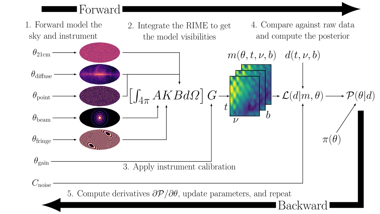
Figure 1: A flowchart describing a Bayesian RIME forward model, starting with the model parameters (left column) and ending with the posterior probability of the parameters given the observed data (right). These parameters could include, for example, the 21 cm signal ($\theta_{\rm 21cm}$), diffuse foregrounds ($\theta_{\rm diffuse}$), point source foregrounds ($\theta_{\rm point}$), antenna beam responses ($\theta_{\rm beam}$), antenna separation vectors ($\theta_{\rm fringe}$), direction-independent antenna gains ($\theta_{\rm gain}$), and a noise covariance of the data ($C_{\rm noise}$). Note that in this work we only treat $\theta_{\rm 21cm}$, $\theta_{\rm diffuse}$, and $\theta_{\rm beam}$ as free parameters, and treat $\theta_{\rm fringe}$, $\theta_{\rm gain}$ as both fixed and known. Wrapping this forward model with a reverse-mode automatic differentiation engine allows us to compute gradients of the posterior with respect to the model parameters after completing a forward pass.

3 Model Parameterization

Here we discuss our choice of parameterization for the components in our forward model, as well as the specifications for our mock HERA observations. In what follows, we will specify a data model for 21 cm intensity mapping at EoR redshifts, however, note that many of these parameterization choices are equally valid for low redshift 21 cm intensity mapping as well. Furthermore, the exact choice of parameterization may be context-dependent, and the process of selecting an optimal parameterization for a given telescope design is still an area of study. Also note that the process of model selection, or determining the degrees of freedom of the model, is a critical question that can be addressed by computing the Bayesian evidence factor in Equation 10 (e.g. Sims & Pober, 2020; Murray et al., 2022). However, this is computationally very expensive, particularly for the large number of parameters used in our forward model, and we defer exploration of this topic to future work.

As a concise summary, the parameters of our forward model that we actually optimize in this work include:

1. Antenna Primary Beam Response – We model the anntena primary beam total power response pattern (assumed to be shared by all antennas) with 75 (real-valued) spherical harmonic angular modes ($\ell_{\rm max}=40$ and $m_{\rm max}=6$) and 5 orthogonal polynomial modes across frequency, for a total of 385 parameters. We set a Gaussian prior on the beam in real space centered at the fiducial model, with a variance that yields $1\sigma$ beam fluctuations at roughly -25 dB, which is generally consistent with our prior knowledge of antenna primary beams (Line et al., 2018; Nunhokee et al., 2020).

2. Foregrounds – We model the (diffuse + point source) foregrounds with spherical cap harmonic modes (discussed below) up to $\ell_{\rm max}=160$, which covers the full horizon-to-horizon observable sky given HERA’s observing coordinates. We use 12,104 harmonic angular modes and 3 orthogonal Legendre polynomials across frequency, for a total of 36,312 (complex-valued) parameters. We adopt a Gaussian prior on the spherical harmonic coefficients that translates to a $\sim 5\%$ uncertainty on the starting fiducial foreground map, which is roughly consistent with our current understanding of the low-frequency foreground distribution (Zheng et al., 2017).

3. EoR Signal – We model the EoR signal with spherical stripe harmonic modes (discussed below) out to the same angular resolution as the foreground model ($\ell_{\rm max}=160$), which covers $\sim 4000$ square degrees across a drift-scan observing mask tracking the main field-of-view of the simulated HERA observations. We use 1,302 harmonic modes to model the angular dimension and 40 orthogonal polynomials for the frequency dimension for a total of 52,080 complex-valued parameters. We set a weak, mean-zero Gaussian prior on the harmonic coefficients, with a variance that is ten times greater than the variance of the mock 21 cm model used as the true underlying signal. This is meant to act as a minimally informative prior model, while still regularizing the modes to prevent them from taking on unrealistic values that would exceed current upper limits.

In total, our forward model contains roughly $\sim 88,000$ parameters across the instrument, foreground, and 21 cm signal components.

3.1 Array Model and Mock Observations

We use a condensed version of the HERA array as a prototype for testing our framework, shown in Figure 2. This consists of 91 antennas packed in a hexagonal fashion with 14.6 meter spacing between antennas, similar to the HERA design without the split-core feature (DeBoer et al., 2017). For this proof-of-concept study, we will only analyze data from baselines with lengths between $0<|\bm{b}|<60$ meters, thus excluding the auto-correlation visibilities ($|\bm{b}|=0)$ and the long baseline visibilities. The baseline cut is mainly for computational reasons due to the limited angular resolution of our foreground model; however, even with this baseline cut we preserve nearly 80% of the array’s power spectrum sensitivity between $0<k<0.35\ h\ {\rm Mpc}^{-1}$, assuming we’ve applied a horizon-wedge FG filter that is similar in specification to the pessimistic foreground case in Pober et al. (2014). This leaves a total of 30 unique baseline vectors that we simulate via Equation 1, which are then broadcasted to 1,785 physical baselines that are used as the model visibilities. This distribution of baseline lengths (combined with the frequency band described below) cover transverse Fourier modes between $0.004\leq|k_{\perp}|\leq 0.016\ {\rm Mpc}^{-1}$.

Our simulated frequencies span a 10 MHz bandwidth from 120 – 130 MHz, yielding a central redshift of $z\sim 10.4$ for the 21 cm line. This aligns with one of the main cosmology observing bands in HERA Collaboration et al. (2022). We simulate the data with a spectral resolution of roughly 222 kHz, which is somewhat more coarse-grain than typical 21 cm experiments; however, in this study we are mainly aiming to recover intermediate $k_{\parallel}$ modes, largely because the high $k_{\parallel}$ modes of most EoR models (i.e. $|k|>1\ {\rm Mpc}^{-1}$) are nearly entirely noise dominated, even for second-generation 21 cm experiments. A 10 MHz bandwidth with 222 kHz spectral resolution allows us to model cosmological line-of-sight Fourier modes between $0\leq|k_{\parallel}|\leq 0.75\ {\rm Mpc}^{-1}$, however, as noted above, we employ a frequency-based high-pass filter that eliminates power in the visibilities for $|k_{\parallel}|\leq 0.1\ {\rm Mpc}^{-1}$

Lastly, our mock HERA dataset is simulated along a contiguous 6-hour drift scan from a local sidereal time (LST) of $0<t<6$ hours, which tracks right ascensions of $0<\alpha<90$ degrees at a fixed declination of -30.72 degrees. This LST range covers the main fields-of-interest used in previous HERA results (HERA Collaboration et al., 2022; The HERA Collaboration et al., 2022). We simulate 68 time integrations evenly spaced throughout the 6-hour interval, resulting in a time difference of 5 minutes between distinct snapshot observations. While this is much longer than a typical observing cadence of real HERA data (on the order of tens of seconds), it is still below HERA’s beam-crossing time of roughly 30-minutes. This allows us to effectively interpolate between time integrations without significant loss of signal if needed. Also note that the final time binning cadence in recent HERA results (after calibration) are on the order of 5 minutes (HERA Collaboration et al., 2022). Figure 3 shows the sky regions used for modeling the foreground and EoR sky signals (top), showing how the diffuse model covers the entire observable sky from HERA’s coordinates, while the EoR model need only cover the main FoV of the drift-scan observations. It also shows the maximum primary beam response throughout the drift-scan observations (bottom), demonstrating that while most of the telescope’s sensitivity is contained within a stripe at fixed declination, the full observable sky is still measured at attenuations of $10^{-3}-10^{-4}$, which is enough to allow bright, off-axis foregrounds like the galactic plane to dominate the intrinsic EoR 21 cm amplitude in the visibilities.

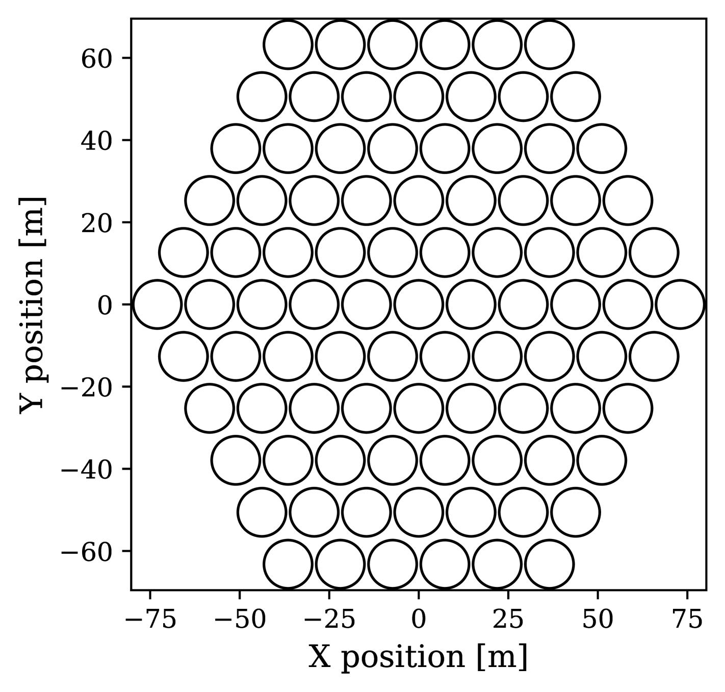
Figure 2: The modified HERA-91 array layout adopted in this work. The array consists of 91 antennas with 14.6-meter spacing. Note that in this work we only simulate baselines with lengths from $0<|\bm{b}|<60$ meters due to constraints on the angular resolution of our adopted sky model; however, this baseline cut still preserves nearly 80% of the total power spectrum sensitivity of the array after foreground wedge filtering.

3.2 Foreground Model

The dominant form of unpolarized astrophysical foregrounds come from non-thermal synchrotron radio emission in the galaxy and from extragalactic sources. Synchrotron continuum follows a powerlaw form of $\nu^{-\alpha}$ with a spectral index of $\alpha\sim 2.2$ (Condon, 1992; Haslam et al., 1982; Remazeilles et al., 2015). As a consequence of the power-law form, these foregrounds are particularly bright at the low radio frequencies used for 21 cm cosmology measurements, reaching up to $10^{5}$ times brigher than the expected 21 cm cosmological signal. A blessing of the power-law form, as discussed previously, is the assumed smoothness of the continuum as a function of frequency. However, the angular distribution of the foregrounds is more complex.

Considerable effort has gone into improving our understanding of these foregrounds for 21 cm cosmology science, particularly at the relatively less-studied frequency bands below 1000 MHz. This includes surveys of the vast population of radio point sources (e.g. Cohen et al., 2007; Hurley-Walker et al., 2017; Riseley et al., 2020; Hurley-Walker et al., 2022), surveys of the diffuse emission from the galaxy (e.g. Haslam et al., 1982; de Oliveira-Costa et al., 2008; Remazeilles et al., 2015; Zheng et al., 2017; Dowell et al., 2017; Eastwood et al., 2018; Mozdzen et al., 2019; Spinelli et al., 2021) and their polarized structures (Jelić et al., 2010; Moore et al., 2013; Nunhokee et al., 2017), and studies of individual, nearby resolved radio galaxies, like Fornax A (McKinley et al., 2015; Line et al., 2020). These synergies have been highly beneficial to the field as a whole, a recent example being how the HERA experiment leveraged the GLEAM survey as a key component in its absolute calibration pipeline (Kern et al., 2020b).

Recently it has become increasingly clear that robust foreground modeling requires a model of the full sky, as opposed to simply the main field-of-view (Pober et al., 2016; Bassett et al., 2021). In particular, diffuse foregrounds near the observer’s horizon creates the now well-studied phenomenon known as the pitchfork effect (Thyagarajan et al., 2015a), which has been observed in simulations (Kern et al., 2019; Lanman et al., 2020; Charles et al., 2023) and in the raw data of a variety of 21 cm telescopes (Thyagarajan et al., 2015b; Kern et al., 2020a; Rath et al., 2024). The pitchfork effect is particularly troublesome because the foregrounds manifest in the visibilities on the boundary of the foreground wedge at $|\tau_{\rm horizon}|$, and are easily leaked into the EoR window from instrumental chromaticity.

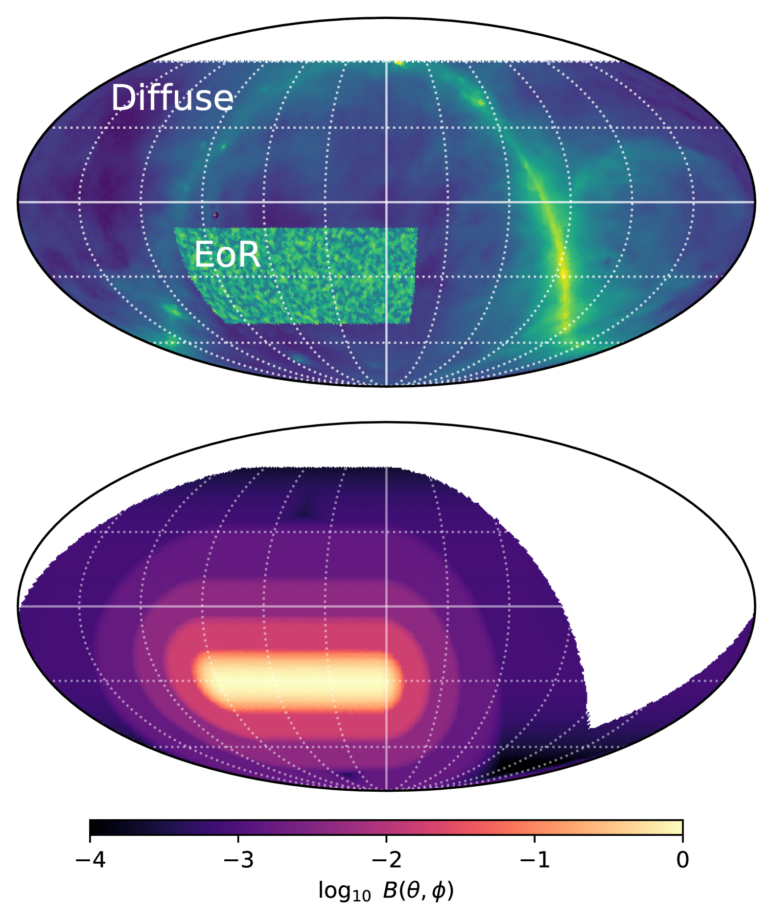
Figure 3: Top: We plot the angular coverage of our foreground model, which spans the full observable sky from HERA’s coordinates (diffuse). We also show the EoR sky model coverage, which tracks a smaller “stripe” across 120 degrees in right ascension at fixed declination. The EoR model amplitude is artificially boosted for visual clarity. Bottom: The maximum primary beam amplitude across the full 6 hour simulated drift-scan observation. This shows the maximum response of the telescope at each sky pixel over the course of the observations, showing that while most of HERA’s sensitivity is confined within a narrow stripe on the sky, it is still sensitive to bright, off-axis foregrounds at an attenuation of $\sim 10^{-3}-10^{-4}$, which is enough to dominate the intrinsic EoR signal in the simulated visibilities.

Our foreground model therefore spans the entire observable sky from HERA’s coordinates (Figure 3). We start with a fiducial model of the diffuse sky from the Global Sky Model catalogue (Haslam et al., 1982; de Oliveira-Costa et al., 2008; Remazeilles et al., 2015; Zheng et al., 2017), specifically the updated 2016 model (Price, 2016), which combines low-frequency measurements of the sky into a series of best-understanding maps at our observing frequencies. Note that while some care has gone into removing different telescope artifacts and bright, extended radio sources in constructing the GSM (Remazeilles et al., 2015), the model still contains a background extragalactic point source distribution.

After evaluating the GSM at each of our observing frequencies, we interpolate the foreground map onto an fixed, equal-area rectangular grid in right ascension and declination with an effective cell resolution of 0.5 degrees, which is similar to a HEALPix NSIDE 128 resolution. This converts the continuous foreground sky brightness distribution with units of specific intensity into pixelized cells with units of flux density, specifically Jansky. This is akin to our RIME integral pixelization in Equation 3, with the grid extending over the entire observable sky from HERA’s coordinates (Figure 3).

We parameterize the angular response of the foregrounds in a spherical harmonic basis, using the spherical cap harmonic formalism (see Appendix A). Briefly, the spherical cap harmonics (Haines, 1985) are a modified spherical harmonic basis that is complete and orthogonal on the spherical cap (as oppposed to the full sphere). This allows for a compressed basis for modeling signals on the cut sky, with the tradeoff being non-integer-valued $\ell$ modes. The forward transform of the angular coefficients into map space is defined as

$$B^{\rm fg}(\hat{s},\nu)=\left|{\rm Re}\left(\sum_{\ell m}^{\ell_{\rm max}}Y_{\ell m}^{\rm fg}(\hat{s})a_{\ell m}^{\rm fg}(\nu)\right)\right|,$$ (11)

where $B^{\rm fg}(\hat{s},\nu)$ is the real-valued, non-negative flux density of the pixelized foreground sky, $Y_{\ell m}^{\rm fg}$ are the complex-valued spherical cap harmonics as a function of sky angle, $a_{\ell m}^{\rm fg}(\nu)$ are the spherical cap harmonic coefficients as a function of frequency channel, and the sum runs over all $\ell$ and $m$ modes up to $\ell_{\rm max}$. Note that due to real-valued nature of the unpolarized foreground sky, we can throw out all negative $m$ modes in $Y_{\ell m}$ and simply multiply the $m>0$ fitted coefficients by a factor of two when taking the forward transform. In matrix form, we can solve for the best-fit harmonic coefficients given a map of the foreground sky via their least squares solution, given as

$$\hat{\bm{a}}=(\bm{Y}^{T}\bm{Y})^{-1}\bm{Y}^{T}\bm{B},$$ (12)

where $\bm{B}$ is the matrix of foreground maps in $\mathbb{R}^{N_{\rm pix}\times N_{\rm\nu}}$, $\bm{Y}$ is a matrix of spherical cap harmonic modes in $\mathbb{C}^{N_{\rm pix}\times N_{\rm modes}}$ and $\hat{\bm{a}}$ are the best-fit harmonic coefficients in $\mathbb{C}^{N_{\rm modes}\times N_{\nu}}$. We model all $\ell\ \&\ m$ modes up to an $\ell_{\rm max}=160$ cutoff for a total of 12,104 coefficients, beyond which the telescope is not particularly sensitive given the maximum baseline in our data and the observing frequencies. Note that the choice of an effectively band-limited model of the diffuse sky given the angular resolution of the telescope means that the foreground model acts effectively as a joint diffuse and point source model. The desire to have a band-limited foreground model in this work is what drives the maximum baseline cutoff of 60 meters, beyond which the number of foreground parameters becomes cumbersome to work with (but perhaps not technically computationally infeasible). Future work will explore other angular parameterizations that may enable a higher $\ell_{\rm max}$ cutoff.

The frequency axis is parameterized with a second-order orthogonal Legendre polynomial (3 coefficients) that enables recovery of the GSM powerlaw-like structures down to a fractional error of $10^{-5}$ over our 10 MHz observing bandwidth. The forward transform from the polynomial coefficient domain into the frequency domain is given as

$$a_{\ell m}^{\rm fg}(\nu)=\sum_{k=0}^{2}X_{k}^{\rm fg}(\nu)\ \tilde{a}_{\ell mk}^{\rm fg},$$ (13)

where $X^{\rm fg}_{k}(\nu)$ are the foreground Legendre coefficients and $\tilde{a}_{\ell mk}$ are the fully compressed foreground parameters. This leads to a total of 36,312 complex-valued parameters for our foreground model.

The native GSM model acts as our starting fiducial model of the low-frequency foreground sky. Fitting the harmonic and Legendre modes to these multi-frequency maps creates our initial parameter vector, $[\tilde{\bm{a}}^{\rm fg}_{\ell mk}]_{0}$, which acts as our starting point before optimization. To simulate a mock HERA observation we perturb the model about this starting point to act as a pseudo “ground truth” that is assumed to be a priori unknown. We do this by adding random Gaussian noise to the fiducial set of coefficients via

$$[\tilde{\bm{a}}_{\ell mk}^{\rm fg}]_{\rm truth}=[\tilde{\bm{a}}_{\ell mk}^{\rm fg}]_{0}+\bm{n}_{\ell mk},$$ (14)

where $\bm{n}_{\ell mk}\sim\mathcal{N}(0,[\sigma_{\rm prior}^{\rm fg}]^{2})$. We tune the amplitude of the noise such that it yields a forward modeled foreground map that has a residual fractional standard deviation that is $\sim 5\%$ of the fiducial foreground map amplitude, which is roughly consistent with our current understanding of low-frequency foregrounds (Zheng et al., 2017). In other words, we tune the noise amplitude $\sigma_{\rm prior}^{\rm fg}$ such that the standard deviation of the ratio $B_{\rm truth}^{\rm fg}/B_{\rm fiducial}^{\rm fg}$ is roughly 0.05. Finally, we set a Gaussian prior directly on the harmonic coefficients with a mean of $[\tilde{\bm{a}}_{\ell mk}^{\rm fg}]_{0}$ and a diagonal covariance matrix with a scalar amplitude of $[\sigma_{\rm prior}^{\rm fg}]^{2}$.

Lastly, we have a few final notes about our foreground parameterization for the avid practitioner. In particular, the bottleneck in the foreground forward model transform is the angular transform by the spherical cap harmonic matrix $\bm{Y}$, which for the specifications listed above would make it a 36,000 $\times$ 153,360 matrix, requiring 45 GB of RAM to store in computer memory (assuming a double precision, complex floating point data type). This is particularly cumbersome when running GPU-accelerated automatic differentiation as the matrix needs to be stored in GPU memory, which is significantly more limited compared to a generic CPU cluster. However, one can significantly decrease the size of this matrix by making it separable along the right ascension and declination axes, which is possible if we choose a uniform, rectangular grid sampling. In this case, the foreground forward transform can be written as

$$B^{\rm fg}(\hat{s},\nu)=\left|{\rm Re}\left(\sum_{\ell m}\Theta_{\ell m}^{\rm fg}(\theta)\Phi_{m}^{\rm fg}(\phi)\sum_{k}X_{k}^{\rm fg}(\nu)\tilde{a}_{\ell mk}^{\rm fg}\right)\right|,$$ (15)

where $\theta$ and $\phi$ are spherical polar and azimuthal angles, respectively, $\Theta_{\ell m}(\theta)$ are the Associated Legendre polynomials, and $\Phi_{m}(\phi)$ are the standard Fourier series (see Appendix A for more details). Having made the forward transform separable onto a rectangular grid of points in $(\theta,\phi)$, we need only store $\Theta_{\ell m}(\theta)$ of size $N_{\theta}$ and $\Phi_{m}(\phi)$ of size $N_{\phi}$, which are both considerably smaller than the $N_{\theta}\times N_{\phi}$ dimensionality of $Y_{\ell m}^{\rm fg}(\theta,\phi)$.

3.3 Cosmological 21 cm Signal Model

To model the cosmological 21 cm signal from the EoR, we first run a semi-numerical simulation of the 21 cm differential brightness temperature signal $\delta T_{21}$ using the 21cmFAST code (Mesinger et al., 2011). We use the default astrophysical and cosmology parameters found in the version-2 code (https://github.com/andreimesinger/21cmFAST), which puts the 21 cm reionization history in agreement with existing probes at the end of reionization (e.g. Park et al., 2019). We simulate a volume with side length $L=800$ Mpc and periodic boundary conditions with a cell resolution of 1 Mpc. Next, we band-limit the simulations by applying a Sinc filter that removes signal above $k\sim 0.75\ {\rm Mpc}^{-1}$, which is the largest Fourier wavemode probed given our frequency channelization. Next we use the “tile-and-interpolate” procedure of converting the simulation box output onto a series of full-sky maps (Kittiwisit et al., 2022). To do this, we tile the 21 cm simulation box in 3D space out to the line-of-sight comoving distance of our observations between $10<z<10.8$, and peform nearest neighbor interpolation onto a high resolution HEALpix grid of NSIDE 2048. We then apply a smoothing filter to bandlimit the maps before interpolating onto the 0.5-degree rectangular grid used for the foreground model. However, in this case, we only use a small cutout of the main field-of-view of the HERA primary beam response instead of using the full observable sky (see Figure 3). This spherical stripe region spans 120 degrees in right ascension and 40 degrees in declination, covering the sky where the primary beam remains over 1% of its peak value throughout the drift-scan observations. We need only model the EoR signal over this smaller area because the vast majority of the cosmological signal enters through this region of the sky due to primary beam attenuation in the far sidelobes.

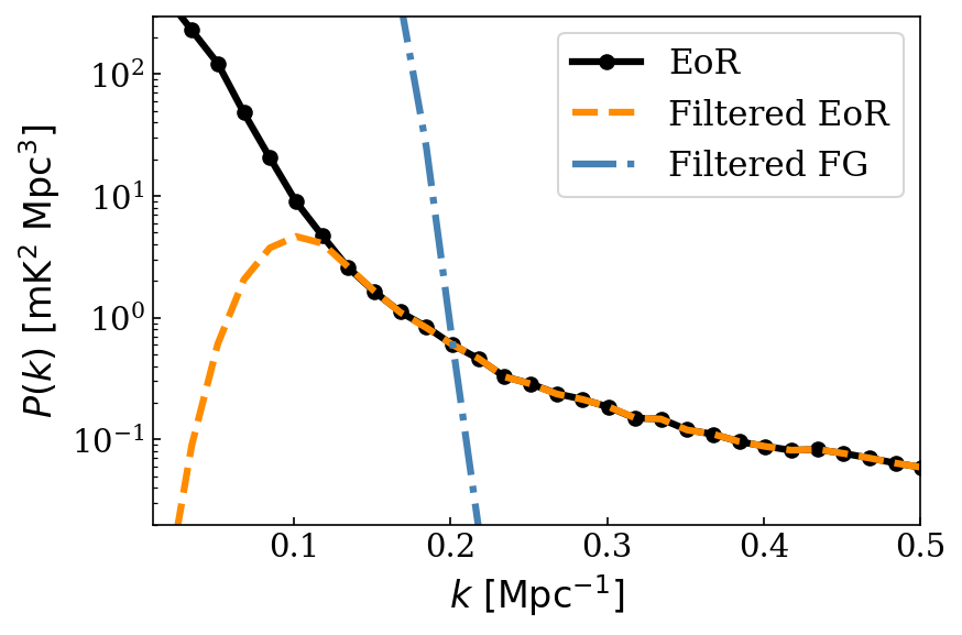
Figure 4: Comparison of a 21 cm power spectrum produced from forward-modeled interferometric visibilities of an EoR sky model (black), and a power spectrum produced from the same visibilities having applied the delay filter (orange-dashed) from Equation 4. The filter suppresses signal in the power spectrum for $k\leq 0.1\ {\rm Mpc}^{-1}$ and leaves other Fourier modes intact. We also plot a power spectrum from the (delay filtered) foreground component of our forward model to demonstrate the range of Fourier modes that would be contaminated without any sort of foreground subtraction, which includes effects from the instrumental response.

We parameterize the 21 cm EoR sky signal with the spherical stripe harmonics (SSH), introduced in Appendix A. Like the spherical cap harmonics, the SSH are a modified version of the spherical harmonics that form a complete and orthogonal basis but for a spherical stripe geometry, sometimes also known as a spherical segment (see Figure 3). This allows us to form a sparse basis given our observing mask while retaining certain statistical properties such as band-limited completeness. We review the SSH and its 3D analog, the spherical stripe Fourier-Bessel formalism, in detail in Appendix A. We model the EoR signal up the same $\ell_{\rm max}=160$ bandlimit of the foreground model, resulting in 1,302 complex-valued coefficients, significantly less than the $\sim$12,000 modes used for the full-sky foreground map with the same $\ell_{\rm max}$.

Like the foreground model, we decompose the harmonic transformation into separable polar and azimuthal transformations, while also using the same equal-area, 0.5 degree resolution sampling pattern as the foreground model. However, unlike the foreground model, we do not limit the sky maps to be non-negative. This is because we are modeling the differential brightness temperature, $\delta T_{21}$, relative to the CMB temperature. Although the total sky brightness is still a non-negative quantity, in practice, $\delta T_{21}$ will never be negative enough to drive the total sky brightness to a negative quantity given our prior model.

For the frequency axis we also use a set of orthogonal Legendre polynomials similar to the foreground model, but now use 40 coefficients to be able to capture the fine frequency fluctuations found in the 21 cm signal. This leads to a total of 52,080 complex-valued parameters for the EoR component of the data model. Thus, our full forward transformation from coefficient space to map space for the 21 cm sky model is given as

$$B^{21}(\hat{s},\nu)={\rm Re}\left(\sum_{\ell m}\Theta_{\ell m}^{\rm 21}(\theta)\Phi_{m}^{\rm 21}(\phi)\sum_{k}X_{k}^{\rm 21}(\nu)\tilde{a}_{\ell mk}^{\rm 21}\right).$$ (16)

The true coefficients for the 21 cm mock observation, $[\tilde{\bm{a}}^{21}_{lmk}]_{\rm truth}$, are computed by fitting them to the simulated 21 cm maps described above. Because there are no direct constraints on the EoR 21 cm field to date, our initial starting model for the 21 cm field is taken to be a vector of zeros. We set a weakly informative prior on the complex-valued 21 cm harmonic parameters with a mean of zero and a variance that is ten times times greater than the variance of the fitted truth parameters. This acts as a minimally informative prior model for the currently weakly constrainted 21 cm field, while still regularizing them to prevent them from taking on unrealistic values that would exceed current upper limits on the signal.

In Figure 4 we show the 21 cm power spectrum generated by the described EoR model. We also show the impact of the delay filter described in subsection 2.1, where to do so we have forward modeled the EoR sky model into a set of visibilities, applied the delay filter, and then estimated the power spectrum from the visibilities (discussed in subsection A.5). We see, as expected, a sharp cutoff in power at $k\leq 0.1\ {\rm Mpc}^{-1}$ for the filtered dataset, while other modes remain untouched.

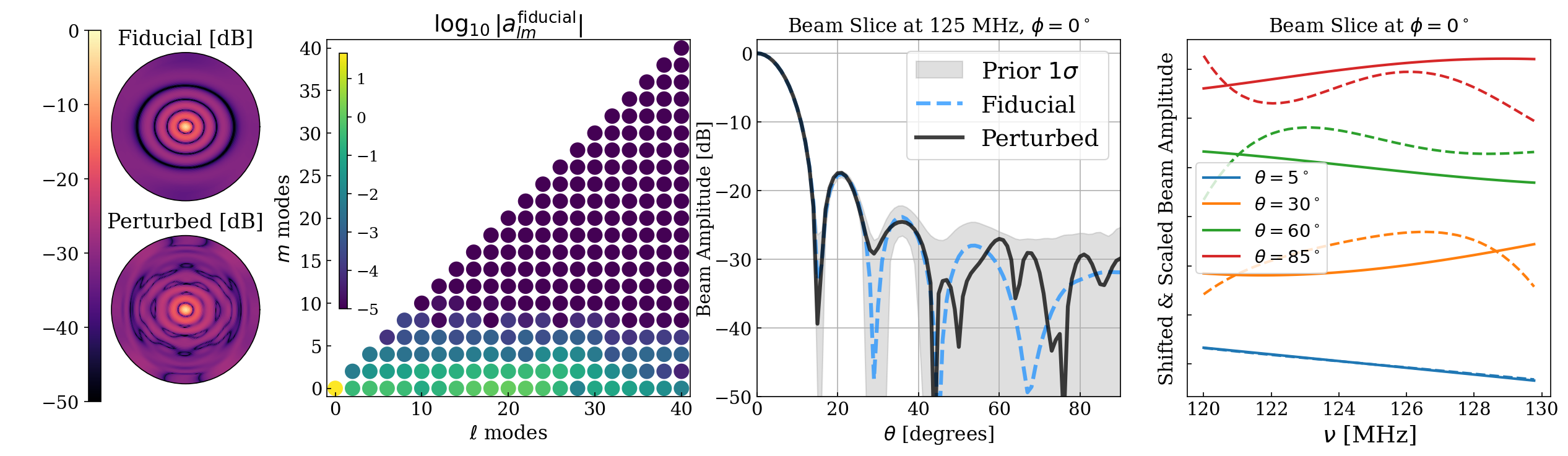
Figure 5: The fiducial and perturbed primary beam response as a function of angle and frequency. Left: Polar projection of the total power beam response at 125 MHz for the fiducial (top) and perturbed (bottom) beam in decibels. Center-Left: The log amplitude of the $a_{lm}$ decomposition of the fiducial beam, showing compression of the beam to low $m$ modes. The hemispherical cap harmonics allow even-valued sampling of $l$ modes, while the assumed 180^∘ degree beam symmetry allows even-valued sampling of $m$ modes and the real-valued nature of the beam allows us to drop negative $m$ modes (they are just complex conjugates of positive $m$ modes), resulting in even further compression. Taking all $a_{lm}$ modes for $m\leq 6$ and $l\leq 40$ results in just 78 real-valued parameters for the beam’s angular dimension. These 78 parameters fit the fiducial modified Airy pattern with a residual RMS less than $10^{-4}$. Center-Right: A slice through the beam amplitude of the fiducial beam (black) and the perturbed beam (red-dashed) in decibels, showing fairly complex structure in the perturbed beam, especially at large zenith angles. We also show the $1\sigma$ width of the prior (gray shaded) centered on the fiducial beam model. Right: A slice through the beam amplitude across frequency at fixed zenith angle (artifically normalized and offset for visual clarity), demonstrating the kind of non-trivial frequency structure found in the perturbed beam (dashed) relative to the fiducial beam (solid).

3.4 Antenna Primary Beam Model

The antenna primary beam response is one of the leading instrumental systematics for 21 cm cosmology, and deserves particular attention (e.g. Shaw et al., 2014; Sokolowski et al., 2017; Tauscher et al., 2018; Line et al., 2018; Kim et al., 2023). Here we adopt a single model for all antennas (sometimes referred to as the “average beam”), which has both angular and frequency degrees of freedom.

Our fiducial beam model is modeled as an Airy disk, which is a good first-order approximation of the HERA antenna response given that the dish carves out a circular aperture. However, we make a slight modification to account for the natural squashing of the beam along the east or north direction (for the east or north-oriented feed, respectively) that arises from the response of the feed. Our modified Airy disk function is written as

$$A(\theta,\phi,D_{\rm ew},D_{\rm ns},\nu) =2J_{1}(x)/x$$ (17)

where

$$x =[D_{\rm ns}+|\sin(\phi)|^{2}(D_{\rm ew}-D_{\rm ns})]\sin(\theta)\pi\nu/c,$$ (18)

and $J_{1}$ is the Bessel function of the 1st kind of order 1. Here, we replace the aperture diameter in the standard Airy disk function with an “effective” diameter that looks larger or smaller depending on the azimuth angle, creating the squashing effect. The square of this function is used as a model of the total power of the antenna primary beam. We defer modeling the polarized primary beam reponse to future work.

While the modified Airy function represents our fiducial (or starting beam model), the “truth” beam model used in simulating our mock, raw dataset is a perturbation about this fiducial model. To generate this perturbation, we decompose the beam model using the spherical cap harmonic formalism (Haines, 1985). In our case, we assume the beam model response covers the full hemisphere above the observer horizon, with a $\theta_{\rm max}=90^{\circ}$. In effect, this means that we use the standard spherical harmonic basis but truncate the odd $\ell$ modes. In the general case of any spherical cap (not just a hemispherical cap), this would translate to a new set of non-integer $\ell$ modes, as is the case for the foreground model described above. We describe the spherical cap harmonics and their associated spherical stripe harmonics in more detail in Appendix A.

We make one modification to the spherical cap harmonics to enable easier fitting to real beam data. First, based on our definition of the primary beam in Equation 1, the total power beam is a unitless quantity that is normalized such that the zenith pointing ($\theta=0^{\circ}$) should be equal to one. However, all of the $m=0$ spherical harmonic modes have a non-zero response at $\theta=0^{\circ}$, meaning there is a tight degeneracy between these modes when fitting the beam near boresight. We could set a very tight prior on our beam amplitude at $\theta=0^{\circ}$ to enforce this property, however, experimentation has shown this creates a posterior that is difficult optimize. Instead, we reparameterize the $m=0$ modes by replacing the $\ell=0$ monopole mode with a Gaussian function that is fit to the envelope of the beam’s main lobe. We then subtract this function from all other $m=0$ modes, such that all modes (except for $\ell=0$) go to zero for $\theta\rightarrow 0^{\circ}$. We then leave the $\ell=0$ mode fixed and only fit $\ell>0$ modes when optimizing for the beam shape. The angular parameterization is therefore defined as,

$$A(\hat{s},\nu)=\left|\sum_{lm}Y_{lm}^{\rm beam}(\hat{s})\ a_{lm}^{\rm beam}(\nu)\right|,$$ (19)

where $A(\hat{s})$ is the total power primary beam in Equation 1. We use an absolute value operator to enforce the intrinsic non-negativity of the total power beam. One could also enforce this by modeling the log power beam, or by setting a non-negative prior on the angular representation of the beam. Based on experimentation, however, we found that taking the absolute value was the most efficient way to enforce this property without degrading the natural sparsity of the harmonic basis.

To model the frequency dependence of the beam we use a set of orthogonal polynomials defined across the observing bandwidth. Specifically, we use a 4th-order Legendre polynomial that is able to capture the intrinsic frequency structure of the fiducial Airy model down to a fractional RMS of $10^{-5}$. Thus, we represent the frequency dimension of the fitted $a_{\ell m}^{\rm cap}$ harmonic modes as,

$$a_{\ell m}^{\rm beam}(\nu)=\sum_{k}X_{k}^{\rm beam}(\nu)\ \tilde{a}_{\ell mk}^{\rm beam},$$ (20)

where $X_{k}^{\rm beam}(\nu)$ is the design matrix holding the 5 orthogonal Legendre polynomials in our 4th-order polynomial model, and $\tilde{a}_{\ell m}^{\rm beam}$ are the fully compressed modes of our frequency and angularly dependent primary beam model.

Figure 5 shows the spherical harmonic decomposition of the this fiducial Airy model, showing good compression of the beam in harmonic space with $m\leq 6$ and $\ell\leq 40$. Furthermore, we achieve even further compression from the fact that we sample even-valued $\ell$ modes due to the hemispherical cap harmonics; we sample even-valued $m$ modes due to the assumed $180^{\circ}$ symmetry of the beam, and we sample only positive $m$ modes because the power beam is intrinsically real-valued. This results in the beam being well-compressed down to only 78 modes given the $\ell m$ cuts described above, which we find can represent the fiducial beam down to a fractional RMS of $10^{-4}$.

To generate our perturbed beam model (i.e. the a priori unknown “truth” beam that we will aim to solve for from the data), we take the $\ell m$ cuts described above and add random Gaussian noise to them, tuned to create fluctuations in the beam amplitude at roughly the -30 dB level (Fagnoni et al., 2020). Figure 5 shows this perturbed beam, demonstrating the complex angular and frequency structure one might expect from a real antenna response located in the field. Furthermore, we show the frequency response of the beam, demonstrating the perturbed beam’s more complex frequency structure relative to the fiducial model that looks visually In total, the primary beam model holds 5 frequency degrees of freedom and 77 angular degrees of freedom (not including $\ell=0$) for a total of 385 parameters.

Due to the differentiable nature of the forward model, we can enact priors on the beam in both harmonic space on the $a_{\ell m}$ modes, as well as in real space where our intuition of the beam is actually gleaned. In this work we set a Gaussian prior on the beam in real space centered at the fiducial beam with a variance that is tuned to yield fluctuations in the beam at the -25 dB level, demonstrated through prior predictive checks. This is a fairly realistic assumption for real low-frequency telescopes (Line et al., 2018; Nunhokee et al., 2020), and basically says that while we may have confidence in our theoretical models of the primary beam near zenith, our knowledge of the far sidelobes is effectively unconstrained.

3.5 Noise Model

Thermal noise in the raw data is sourced at the visibility level, and is drawn from a complex-valued normal distribution that is assumed to be uncorrelated between different time bins, frequency bins, and baselines. For thermal noise sourced at the amplifiers in the front end of a radio receiver, this is a very good approximation. We assume a single noise variance for all times, frequenices, and baselines, with an amplitude that is tuned to yield a $\sim 10\sigma$ power spectrum detection of our simulated EoR signal at $k\sim 0.2\ h\ {\rm Mpc}^{-1}$. This is representative of what an early detection by HERA might look like with a single observing season of data (DeBoer et al., 2017). In other words, the covariance of the noise vector $\bm{n}$, which has the same dimensionality of $\bm{y}$ in Equation 3, has a covariance

$$\bm{N}=\langle\bm{n}\bm{n}^{\dagger}\rangle$$ (21)

that is diagonal and scalar, such that $N_{ii}=\sigma_{n}^{2}$.

A slightly more realistic noise model would entail simulating a total-power observation of the diffuse foreground sky to compute the measured sky temperature as a function of frequency and observing time, and adding this with a receiver temperature describing thermal noise originating from the front-end analog system (as in Aguirre et al., 2022). However, the simpler model adopted here allows us to fine tune the noise amplitude for diagnostic purposes, and is more than sufficient to demonstrate the proof-of-concept signal recovery studied in this work.

Note that the delay filtering step applied to the raw and model visibilities (Equation 4) will slightly change the noise properties of the data, with an updated covariance given as

$$\tilde{\bm{N}}=\bm{F}\bm{N}\bm{F}^{\dagger}.$$ (22)

While $\bm{N}$ was a diagonal matrix, $\tilde{\bm{N}}$ need not be, however, due to the fact that $\bm{F}$ is a very narrow high-pass filter, visual inspection shows $\tilde{\bm{N}}$ to be strongly diagonally dominant, and thus we maintain the usage of a diagonal covariance matrix but replace $N_{ii}$ with $\tilde{N}_{ii}$ in the likelihood (Equation 9).

4 Signal Estimation and Posterior Sampling

In this section we demonstrate a proof-of-concept optimization and posterior sampling exercise given our mock HERA observation from a set of a priori unknown “truth” set of model parameters. The goal is to optimize the joint model to the maximum a posteriori (MAP) value, and then to sample the posterior via a Markov Chain Monte Carlo (MCMC) process. After sampling the posterior we are left with an approximation of it that will allow us to effectively marginalize the posterior across our foreground and instrumental nuisance parameters, thus acheiving our goal of characterizing the joint posterior distribution and performing end-to-end uncertainty propagation.

4.1 Posterior Optimization

One of the challenges in optimizing a model like the one described above is the intrinsic degeneracy between different components of our data model. For example, for the same frequency mode, the EoR and diffuse sky models are perfectly degenerate within the main field-of-view. In practice, low-order frequency modes of the foreground model modulated by high-frequency modes of the beam model can also be partially degenerate with higher frequency modes of the EoR model. This is not unique to our end-to-end forward model approach, and is indeed indicative of the challenge of the 21 cm inverse problem. These degeneracies create narrow valleys in the posterior that are difficult for the optimizer to navigate, especially in high dimensions. In our experimentation, we have therefore not suprisingly found the most success by employing 2nd-order optimization routines like the L-BFGS quasi-Newton method over 1st-order approaches liks stochastic gradient descent. The L-BFGS algorithm uses a sparse-Hessian approximation that allows it to better navigate ill-conditioned and high-dimensional parameter spaces like the one presented in this work (Liu & Nocedal, 1989; Nocedal & Wright, 2006).

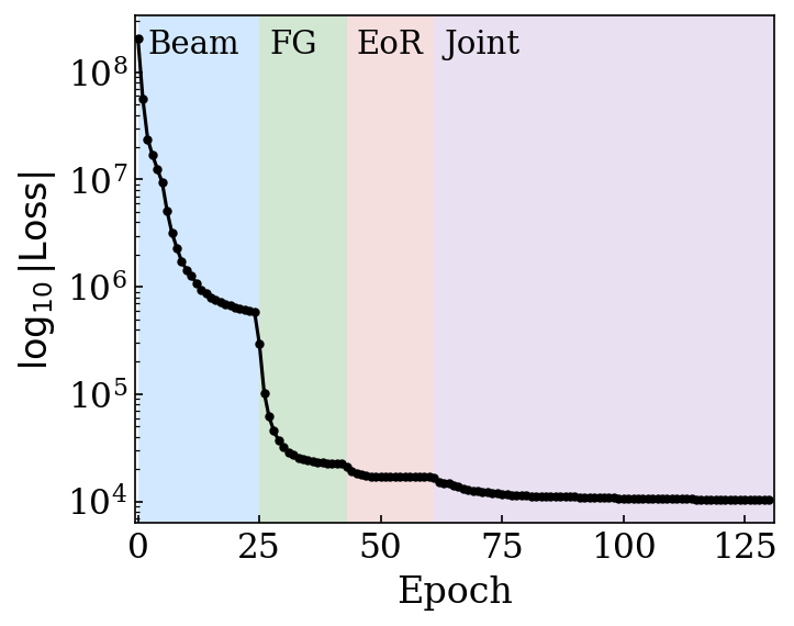
Figure 6: Optimization of the forward model using the quasi-Newton L-BFGS solver, starting with disjoint optimization of each component, followed by a joint optimization. We have thinned the number of epochs for visual clarity. In total we run roughly 100 iterations for each component separately and then run roughly 1000 iterations jointly.

In particular, we have found that there is a strong degeneracy between the $m=0$ mode of the 21 cm sky model and the beam model. Perhaps not surprisingly, this is due to the drift-scan nature of the simulated observations, where the $m=0$ mode of the sky acts as a constant offset in the visibilities as a function of observing time, which is degenerate with the combination of the beam and the foreground model. As a consequence, we remove the $m=0$ modes of the 21 cm model out of the optimization procedure because, without aggressive regularization, they can make the Hessian matrix singular. This does not impact our ability to make an unbiased recovery of the EoR power spectrum, as the final power spectrum (described in subsection A.5) is simply an average over $\ell\ \&\ m$ spherical harmonic modes, and we’ve effectively just set the $m=0$ weight to zero.

To further aid the convergence of the optimization, we first optimize each component independently before performing a joint optimization, running 100 iterations for each component before running roughly 1000 iterations with a joint parameterization. We plot the results of the optimization in Figure 6, showing the decrease in the loss function (in our case the un-normalized negative log posterior) as function of iterations. We see that the beam optimization does the most to bring the model data and raw data into alignment, which highlights its importance in end-to-end signal estimation. We terminate the optimization manually when the $k\sim 0.1\ {\rm Mpc}^{-1}$ modes of the forward modeled EoR visibilities have stabilized.

Running the forward model in a data parallel manner spread across four NVIDIA A100 GPUs results in a runtime of $\sim 0.3$ seconds for a single parameter update step, which involves a forward pass of the model and the backpropagation step. Thus the total time for the optimization described above takes only a few minutes.

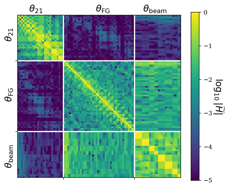
Figure 7: A subset of the diagonal-normalized Hessian matrix across the three components of the forward model, $\widetilde{\bm{H}}$. There are strong off-diagonal entries between the beam and foreground component, and weaker but still non-zero off-diagional entries between the beam and the 21 cm component. Note this does not necessarily represent the cross-covariance between the components, which would be found by inverting the Hessian, but this does give intuition for the degeneracies between the components. Also note that this is only a small subset of the otherwise 80-thousand by 80-thousand Hessian matrix.

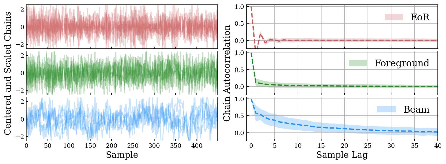
Figure 8: Left: HMC-NUTS chains from Appendix B for the three components of our data model (EoR, foreground, beam). Each chain that is shown represents a random parameter from its associated component, and is centered and scaled for visual clarity. Right: The average autocorrelation for all parameters of a given component (dashed) and their $\pm 1\sigma$ region (shaded). Using Equation 68 on the average autocorrelation for each component (dashed), we compute autocorrelation lengths of roughly (2, 3, 15) for the (EoR, foreground, beam) components, respectively.

4.2 Posterior Sampling

Once we’ve optimized to the maximum a posteriori (MAP) estimate, we’d like to quantify the shape and width of the posterior in order to perform uncertainty quantification. One approximate way we can do this is by quadratically Taylor expanding the posterior about its MAP estimate using the Hessian matrix, which forms a Gaussian approximation to the posterior known as the Laplace approximation. However, a Gaussian approximation to the posterior may be insufficient for noisy data or a posterior distribution that is multi-modal or has complex degeneracies. More standard in the Bayesian inference literature is to sample the posterior via a Markov Chain Monte Carlo (MCMC) method. In particular, the Hamiltonian Monte Carlo (HMC) approach (Duane et al., 1987; Neal, 2011) and its variants such as the No-U-Turn sampler (NUTS; Hoffman & Gelman, 2011) are considered state-of-the-art for complex, high-dimensional Bayesian inference problems. These samplers simulate Hamiltonian dynamics in a dual position and momentum space to make Markov proposals that have low autocorrelation, and thus converge to the underlying posterior distribution more quickly than a random walk Metropolis-Hastings algorithm. See also Jasche & Wandelt (2013); Hernández-Sánchez et al. (2021) for instances of HMC applied to cosmological parameter inference. We refer the reader to Betancourt (2017) for a review of HMC and NUTS.

Although HMC samplers are considered state-of-the-art for many Bayesian inference tasks (Betancourt, 2017), they still often need guidance when tackling high-dimensional and degenerate parameterizations found in real-world applications. To confront these inference problems, it is beneficial to precondition the system with the posterior Hessian matrix, $\bm{H}$ (Girolami & Calderhead, 2011). In the HMC literature, this is known as the Hamiltonian mass matrix, $\bm{M}$, which defines the mapping between the momentum vector and the gradient of the position vector (Neal, 2011). AD-enabled forward models are convenient in that they allow for explicit computation of the Hessian matrix using the computational graph itself. However, even with automatically differentiable gradient calculations, it can still be difficult to compute, store, and invert the full Hessian matrix of the system. As a consquence, it is common to see a diagonal mass matrix used to partially precondition the system.

For our case study, we have found that a diagonal approximations is not effective at enabling efficient exploration of the posterior distribution. Therefore, we use a block-diagonal Hessian matrix to precondition the HMC sampling. We compute dense Hessian matrices for each model component (e.g. EoR, FG, beam) while ignoring their off-diagonal terms, with the only exception being the $\theta_{\rm FG}\times\theta_{\rm beam}$ off-diagonal, which we keep because it is small in size and has outsized influence in the Hessian matrix. We show a small subset of the diagonally normalized Hessian matrix in Figure 7 to demonstrate this. This quantity, $\widetilde{\bm{H}}=\bm{h}^{-1/2}\bm{H}\bm{h}^{-1/2}$ where $\bm{H}$ is the Hessian matrix and $\bm{h}$ is the diagonal of the Hessian matrix, effectively normalizes the diagonal to be one, and thus makes it easier to visualize the importance of the off-diagonal components. The Hessian matrix, being the matrix of second-order derivatives of the negative log posterior, shows strong off-diagonals between the beam and foregrounds, and weaker off-diagonals between the beam and the EoR. Note this does not represent the cross-covariance between the different components of the forward model, which could be computed by inverting the Hessian matrix, but rather gives a sense for the degeneracies between the parameters. Also note that this is only a small subset of the nearly 80 thousand parameters in the full Hessian matrix, and only goes to roughly show the importance of the block diagonal and off diagonals.

Note that to run HMC we only need the Cholesky factor of the adopted mass matrix. In Appendix B we review the quantities needed to simulate HMC trajectories and discuss how to do this in $\mathcal{O}(N^{2})$ time given only the mass matrix Cholesky factor. Future work will explore how to leverage redundant structures in the Hessian matrix to create sparser preconditioners that will enable scaling to even larger parameter dimensionalities.

Having chosen our HMC-NUTS mass matrix, the final two parameters for HMC are the step-size and path-length. We manually tune the step-size to be the largest possible while still returning high acceptance probability (greater than 90%). The path-length parameter is automatically resolved by NUTS’ termination criterion (Hoffman & Gelman, 2011). In practice, we find that the HMC trajectories often terminate between 128 – 256 steps. Finally, we use the biased progressive sampling approach to sample the final ending point of the HMC trajectroy (Betancourt, 2017), which gives preference to points in the trajectory farther away from the initial point.

We run the sampler for 500 iterations, discarding the first 50 due to burn-in. In total the sampling process takes 16 hours to run across 4 GPUs, totalling to 64 GPU hours. A visualization of the resultant HMC chains and their autocorrelation can be found in Figure 8, showing relatively low autocorrelation with an effective sample size (ESS) of over 100 for the EoR component. The foreground component also maintains a low autocorrelation length, while the beam component sees a higher autocorrelation and thus a lower effective sample size (see Appendix B). We speculate that the longer autocorrelation length for the beam model is due to the non-linear absolute value operation applied to the beams during the forward modeling process, making the parameter space slightly more difficult to navigate.

In Figure 9, we show draws from the posterior chains of the beam response, which represents the marginal posterior on the beam model. We see that the posterior draws do a good job representing the true underlying beam response while also capturing the differing levels of uncertainty as a function of polar angle. We also compare the resultant standard deviation of the beam’s marginal posterior, the starting prior, and the conditional posterior (i.e. the posterior holding the foregrounds and EoR parameters constant). As expected, we see the marginal posterior is tighter than the prior, but not as tight as the conditional posterior. This tells us that we are indeed capturing the extra uncertainty in our beam model due to degeneracies between the beam and other components in our model.

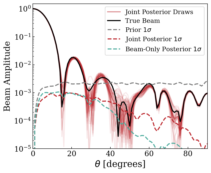
Figure 9: The estimated posterior distribution of the beam at 125 MHz, cut along an azimuthal slice. We plot the true beam response (black) against a representative set of MCMC draws from the forward modeled beam posterior distribution (red solid), showing good agreement of the posterior draws with the underlying ground truth. We also plot the standard deviation of the forward modeled prior distribution (also known as the prior predictive distribution) of the beam (gray dashed), the jointly marginalized posterior predictive distribution (dashed red), and the beam-only marginalized posterior predicive distribution (blue dashed). We see that the posterior is tighter than the prior, as one would expect, and that the variance shrinks near the observer’s horizon (for $\theta\rightarrow 90^{\circ}$), as we intuited before based on the effects of the high-pass delay filter. Furthermore, we see that the beam-only marginalized posterior is indeed tighter than the full, jointly marginalized posterior, indicative of non-neglible correlations between the beam and other components in the data model, as we suspected.

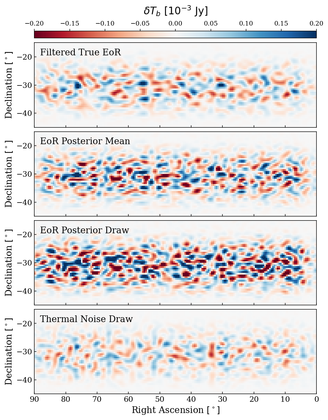
Figure 10: Forward-modeled EoR maps at 125 MHz. These maps come from forward modeling a signal to the full time-ordered visibilities and then applying the imaging step Equation 24. The maps have not been primary beam corrected, so the preceived flux is attenuated near the image boundaries. We show the true underlying EoR signal after high-pass visibility filtering (top), as well as the EoR map corresponding to the mean of the HMC posterior chains (middle-top) and a random draw from the HMC chain (middle-bottom). We also image a thermal noise draw from our visibility noise covariance (bottom). Relative to the true EoR map, the recovered posterior mean appears noisier due to a combination of the thermal noise in the maps as well as degeneracies with the foreground and instrumental components of the forward model.

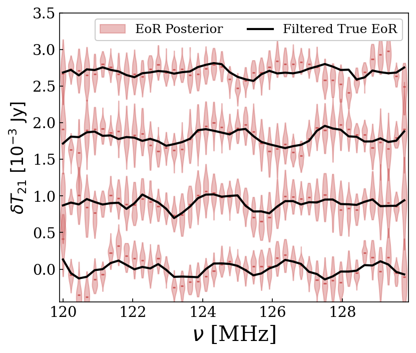
Figure 11: The EoR component of the HMC posterior chains forward modeled and imaged into sky maps, showing a few sight-lines within the main field-of-view. We show the marginal EoR posterior distribution (red) alongside the underlying true EoR signal after delay-filtering and imaging (black). The width of the posterior is driven mainly by marginalized uncertainty from foregrounds and instrument parameters, with a subdominant component coming from the thermal noise in the raw data. The sight-lines have been artificially shifted for visual clarity. This demonstrates that we can estimate the 21 cm marginal posterior at the field level, which can then be projected to a summary statistic if desired.

Next we can inspect the posterior distribution marginalized over the beam and foreground components onto the EoR signal. This is in effect probing the posterior of the 3D EoR signal at the field level, which allows us to capture uncertainty on the maps as well as any summary statistic we might care to form on top of these maps. Recall that so far we have yet to define any kind of formal summary statistic for the EoR field: our optimization and sampling have simply leveraged the forward model that maps signals directly to the complex visibilities. To visualize the EoR component of the MCMC chains we take each EoR sample in the chain and forward model it to the visibility level. Then we apply an imaging step to turn it into a wide-field map. We discuss the mathematics of this step in subsection 4.3 but we will discuss the results here.

Figure 10 shows an example of the maps produced by this process at 125 MHz. Note that the maps have not been primary beam corrected, so they will be naturally attenuated by the edges of the image. We show the true underlying EoR signal imaged after applying the delay filter (top), along with the marginal posterior mean (middle-top), a random draw from the posterior (middle-bottom), and a realization of the thermal noise in the data (bottom). We see there is more effective noise in the posterior mean and draws that comes from the marginalization of uncertainty from the foreground and instrumental parameters. Looking carefully, one can see that the rough features of the filtered true EoR map are indeed preserved in the posterior mean image, particularly nearly the maximum response of the telescope at a declination of -30.72 degrees.

Because we are producing 3D images of the EoR sky signal, we can also look at the data along a line-of-sight at a fixed right ascension and declination. Recall that for an intensity mapping probe the line-of-sight direction is directly mapped to the observing frequency of the telescope. Figure 11 shows a few random sightlines near the peak response of the telescope. We plot the true underlying EoR signal after applying the delay filter (black) alongside the full marginalized posterior (red). This better represents the fact that we are indeed probing the posterior of the EoR signal at the field level, whose per-frequency averages show high correlation with the underlying signal in the data. Given we now have posterior chains of the EoR signal at the map level, we are free to project these to any summary statistic of our choosing.

4.3 Map-making and Power Spectrum Estimation

We use the power spectrum as a summary statistic, which is both well understood and holds a significant amount of the information content in the Cosmic Dawn 21 cm signal (Prelogović & Mesinger, 2024), although future work could explore alternative summaries that exploit non-Gaussian information. There are multiple ways to estimate the 21 cm power spectrum given a set of interferometric visibilities. Some estimators, such as the delay spectrum discussed in subsection 2.2, go straight from the visibiltiies to the power spectrum, while other approaches first reconstruct the sky via a map-making process and then estimate the power spectrum from those maps. There is an expansive literature on interferometric map-making for 21 cm cosmology (e.g. Sullivan et al., 2012; Shaw et al., 2014; Dillon et al., 2015; Eastwood et al., 2018; Morales et al., 2019; Xu et al., 2024), which we will not review in depth here and instead refer the reader to (Liu & Shaw, 2020) for detailed discussions. Recall that all of the optimization and posterior sampling described above relies only on the forward pass of the model (from sky to visibilities) and the backpropagation algorithm. Having already performed the optimization and sampling, we will now use images and power spectra to quantify the results.

4.3.1 Map-making

Briefly, the map-making step produces images of the sky by transposing the forward transformation of the visibility simulation (Equation 3) and multiplying by a user-defined normalization matrix. Let the noisy visibility ($\bm{y}$) for a single frequency channel be written as

$$\bm{y}=\bm{A}\bm{x}+\bm{n},$$ (23)

where $\bm{n}$ is Gaussian noise. Then the generalized map-making solution is defined as

$$\hat{\bm{x}}=\bm{D}\bm{A}^{\dagger}\bm{N}^{-1}\bm{y},$$ (24)

where $\hat{\bm{x}}$ is the estimated map, $\bm{A}$ is the matrix encoding the beam and fringe response in Equation 3, and $\bm{D}$ is a user-defined invertible normalization matrix (Tegmark, 1997; Dillon et al., 2015). The noise in the visibilities is assumed to be drawn from a mean-zero, uncorrelated Gaussian distribution with a covariance of $\bm{N}=\langle\bm{n}\bm{n}^{\dagger}\rangle$. The choice of normalization matrix $\bm{D}$ depends on the desired statistical properties of the map. We can further write down the point spread function (PSF) of the maps,

$$\bm{P}=\bm{D}\bm{A}^{\dagger}\bm{N}^{-1}\bm{A},$$ (25)

which, under an ensemble average of the maps $\langle\hat{\bm{x}}\rangle$, satisfies the following relation

$$\langle\hat{\bm{x}}\rangle=\bm{P}\bm{x}.$$ (26)

Thus $\bm{P}$ describes how the measurement process of the interferometer mixes the intrinsic flux of a map pixel with neighboring pixels. The “optimal” choice of $\bm{D}$ depends on the desired statistical properties of $\hat{\bm{x}}$, but generally the optimal map-making formalism refers to a collection of approaches that retain all of the statistical information encoded in $\bm{y}$. In theory one would choose the maximum likelihood solution $\bm{D}=(\bm{A}^{\dagger}\bm{N}^{-1}\bm{A})^{-1}$, but this is almost never strictly invertible for radio interferometers and thus a range of alternatives exist. Note that if we wanted to include the high-pass Fourier filtering of the visibilities described in subsection 2.1 then the PSF matrix becomes $\bm{P}=\bm{D}\bm{A}^{\dagger}\tilde{\bm{N}}^{-1}\bm{F}\bm{A}$, where recall $\bm{F}$ is the filtering operation, and now $\bm{D}$, $\bm{A}$, $\tilde{\bm{N}}$, and $\bm{y}$ are stacks of themselves for each frequency bin. Many authors choose a simple diagonal normalization matrix that, although does not deconvolve the map, is computationally efficient, and so long as we can compute $\bm{P}$ we can always make faithful comparisons to models of the sky (Dillon et al., 2015). In this work we also use such a diagonal normalization matrix

4.3.2 Power Spectrum Estimation

Having produced maps of the sky we are now prepared to compute their power spectra. Under a flat sky approximation we could take the 2D transverse Fourier transform to generate $\bm{k}_{\perp}$ modes and a 1D line-of-sight transform to generate $\bm{k}_{\parallel}$ modes, however, for large fields-of-view this relationship breaks down as a single line-of-sight does not exist. The appropriate generalization of 3D Fourier transforms on the sphere is the spherical Fourier-Bessel (SFB) formalism, used extensively in wide-field galaxy survey analyses (e.g. Binney & Quinn, 1991; Leistedt et al., 2012; Rassat & Refregier, 2012; Pratten & Munshi, 2013; Grasshorn Gebhardt & Doré, 2021), and recently adapted for intensity mapping experiments (Liu et al., 2016). Here we will use the SFB formalism for power spectra estimation, but do so under the newly defined spherical stripe Fourier-Bessel (SSFB) formalism, which we introduce in Appendix A.

Figure 12: The EoR power spectrum posterior. Left: Power spectra from forward modeling draws from the HMC chain (red), representing the marginal posterior distribution on the EoR power spectrum. These distributions are in good-agreement with the underlying true EoR power spectrum down to the delay-filtering scale of $k=0.1\ {\rm Mpc}^{-1}$, below which the data are attenuated by the filter. We also show the averaged $2\sigma$ level from our mock noise draws, which represents the noise floor in the recovered power spectra (blue-dashed). Right: The maximum a posterior EoR power spectrum divided by the true filtered EoR power spectrum (points). We also show the $\pm 2\sigma$ noise distribution (blue) and EoR marginal posterior (red), the latter of which demonstrates good agreement with the fractional errors observed in the recovered power spectra across all $k$ modes up to $k\sim 0.5\ {\rm Mpc}^{-1}$, above which the data are noise dominated. The sharp increase in uncertainty for $k<0.15\ {\rm Mpc}^{-1}$ is due to the marginalization of uncertainty from the foreground and instrument model onto these modes, achieving our stated goal of computing a fully “end-to-end” errorbar on the power spectrum.

In subsection A.5 we specifically discuss power spectrum estimation within the SSFB formalism, which we will briefly review here. Let the 21 cm temperature field be $T(\bm{r})$ in units of Kelvin. The 3D Fourier transform of the field is written as

$$\widetilde{T}(\bm{k})=\int d^{3}r\ e^{i\bm{k}\bm{r}}\ T(\bm{r}),$$ (27)

with the inverse transform $T(\bm{r})=\mathcal{FT}^{-1}(\widetilde{T}(\bm{k}))$ picking up units of $1/(2\pi)^{3}$ for normalization. The power spectrum is defined as the square of the Fourier-transformed field under an ensemble average, given as

$$\langle\widetilde{T}(\bm{k})\widetilde{T}^{\ast}(\bm{k}^{\prime})\rangle=(2\pi)^{3}\delta^{D}(\bm{k}-\bm{k}^{\prime})P(\bm{k}),$$ (28)

where $\delta^{D}(\bm{k}-\bm{k}^{\prime})$ is the Dirac delta function. Thus we often think of the power spectrum as the square of the Fourier-transformed field.

In the spherical Fourier-Bessel formalism, we have a different representation of the field in Fourier space, one that is given as

$$T_{\ell m}(k)=\int d\Omega dr\ r^{2}j_{\ell}(kr)Y_{\ell m}^{\ast}(\hat{r})T(\hat{r},r),$$ (29)

where $T_{\ell m}(k)$ are the SFB coefficients, $d\Omega={\rm sin}\theta d\theta d\phi$, $Y_{\ell m}$ are the spherical harmonics, and $j_{\ell}$ is the spherical Bessel function of the first kind. To estimate $P(\bm{k})$ using the spherical Fourier-Bessel formalism, we need an analogous relationship between the SFB-transformed field and the power spectrum, which is given in (Liu et al., 2016) as

$$\langle T_{\ell m}(k)T^{\ast}_{\ell^{\prime}m^{\prime}}(k^{\prime})\rangle=k^{-2}\delta^{D}(k-k^{\prime})\delta_{\ell\ell^{\prime}}\delta_{mm^{\prime}}P(k).$$ (30)

Similar to before, we see that we can estimate the power spectrum directly by squaring and binning SFB modes estimated from the maps. In practice, to do this numerically we create SFB transformation matrices that map the pixelized sky to the SFB coefficients and then square them and average them to estimate the 1D power spectrum $P_{k}$. We use a Hann function to apodize the maps along the frequency direction before taking the SSFB transform, which reduces Fourier-space sidelobes when taking the SFB transformation.

When forming the power spectrum as in Equation 30, if the two temperature fields $T_{\ell m}(k)$ and $T_{\ell^{\prime}m^{\prime}}^{\ast}(k^{\prime})$ are drawn with the same thermal noise then we will end up with an additive noise bias term in the power spectrum (Dillon et al., 2014). This can be removed by cross-multiplying maps with different noise statistics, such that they average to zero, or it can be subtracted directly from the final power spectrum given an estimate of the bias. In this work we use the latter approach, using a handful of simulated noise visibilities drawn from the noise covariance to estimate this noise bias term. Note that we never include the actual noise realization in this bias subtraction, only noise realizations drawn from the same covariance.

4.3.3 The 21 cm Power Spectrum Posterior

We are now prepared to take our HMC posterior chains on the EoR component and forward model them to the visibilities, image them into maps, and then estimate their SSFB power spectra. In the left panel of Figure 12 we show the derived marginal posterior on the power spectrum bins (red shaded) and their MAP estimates (black points) alongside the underlying filtered true EoR power spectrum (black line), which we truncate below $k\leq 0.1\ {\rm Mpc}^{-1}$ due to attenuation of the visibility delay filer (Figure 4). For modes above the filter scale, we see good agreement between the recovered posterior distributions and the true power spectrum, which bottoms-out to the noise floor for $k\geq 0.5\ {\rm Mpc}^{-1}$.

The agreement between the estimated power spectrum and the true underlying power spectrum is better captured in the right panel of Figure 12. Here, we show the ratio of the maximum a posteriori (MAP) EoR power spectrum to the true EoR power spectrum (black points), with the shaded regions indicating the marginal posterior $2\sigma$ width (red) and the standard thermal noise $2\sigma$ width (blue). As noted previously, most current 21 cm analyses only compute the thermal noise uncertainty (The HERA Collaboration et al., 2022), which is relatively straightforward to compute, and are unable to account for an end-to-end uncertainty model that we now show here for the first time (red). As expected, this uncertainty increases at a certain $k$ scale (in this case $k\sim 0.15\ {\rm Mpc}^{-1}$), below which the EoR model becomes increasingly degenerate with the combined foreground and beam model. To our knowledge, this is the first demonstration of an end-to-end, marginalized posterior distribution on the 21 cm power spectrum accounting for fluctuations in both foreground parameters and instrumental parameters.

In a practical analysis, one would opt to use this joint uncertainty model when claiming a putative power spectrum detection, making it more robust to the threat of partially degenerate foreground and instrument parameters. For example if we simply used the thermal noise uncertainty model for the power spectrum bins between $0.1<k<0.15\ {\rm Mpc}^{-1}$, the right panel of Figure 12 shows we would produce biased measurements by upwards of $10\sigma$. This is particularly important because these Fourier modes are also the modes that, for many theoretical EoR models (Mesinger et al., 2011), have the largest signal-to-noise ratio. This means they make up the bulk of our total sensitivity and tend to drive astrophysical parameter inference (Breitman et al., 2024), making their robust estimation even more important.

5 Conclusion

Given the difficulty in separating the 21 cm signal from bright foregrounds and complex instrumental systematics, recent years have seen a fresh wave of attention paid to more robust uncertainty quantification, systematic modeling, and the application of Bayesian methods (e.g. Sims et al., 2019; Rapetti et al., 2020; Anstey et al., 2021; Burba et al., 2023; Kennedy et al., 2023; Scheutwinkel et al., 2023; Murphy et al., 2024; Pagano et al., 2024; Glasscock et al., 2024; Wilensky et al., 2024). The overarching aim of these approaches is to be able to more accurately and robustly subtract foregrounds and systematics while also accounting for their degeneracies with the underlying 21 cm signal. However, to date, a unified, end-to-end Bayesian forward model that can marginalize over both foregrounds and the telescope response for an interferometric experiment has yet to be developed. In this work we set out to develop the first end-to-end, differentiable Bayesian forward model for 21 cm cosmology and line intensity mapping (LIM) more generally, called BayesLIM. The framework aims to estimate the joint posterior distribution between a 3D cosmological signal alongside the often degenerate and poorly constrained foreground and instrumental response. This is particularly important for 21 cm LIM due to the presence of overwhelming foregrounds. Although computationally demanding, we show that the advent of high-level automatic differentiation software libraries combined with large-memory graphics processing unit (GPU) computing can make the end-to-end Bayesian forward model a feasible solution in certain cases.

We provide a proof-of-concept on a mock HERA observation where we model the antenna primary beam’s frequency and angle-dependent response alongside a full-sky foreground sky model and a 21 cm sky model. In total the data model contains roughly 80,000 active parameters spanning the three components, with priors that are representative of our current best-understanding of the foreground sky and of low-frequency antenna primary beams. We show we can optimize to an unbiased maximum a posteriori (MAP) solution for EoR Fourier modes $k>0.1\ {\rm Mpc}^{-1}$, and also demonstrate end-to-end uncertainty quantification via Hamiltonian Monte Carlo sampling that for the first time can marginalize the uncertainty from both foreground and instrumental parameters onto the EoR model at the field level. The framework presented here will be key in moving the current state of 21 cm cosmology from setting upper limits to making direct, robust detections of the 21 cm cosmological signal, both for the 21 cm power spectrum and the 21 cm monopole.

In addition, we have presented a novel extension to the spherical harmonic formalism specific to the sky mask used by drift-scan radio telescope observations, which we call the spherical stripe harmonics. These harmonics are a bandlimited-complete and orthogonal basis on the spherical stripe cut sky, and enable an order of magnitude reduction in the number of parameters needed to model a 21 cm sky signal for HERA. We also introduce their 3D analog, the spherical stripe Fourier Bessel formalism (SSFB) for modeling 3D intensity mapped signals and computing power spectra.

While the BayesLIM codebase is expanded and the framework applied to real experimental data, there are a number of areas for improvement going forward. In particular, the inclusion of instrumental systematics like mutual coupling and gain calibration terms could be included for a more realistic end-to-end instrument model. Second, foreground models that include polarized sources as well as bright, extended radio sources like Fornax A will improve model realism when applied to real data. In addition, more efficient posterior sampling, e.g. with neural posterior estimation (Zeghal et al., 2022), will help to tackle larger datasets such as a full HERA array or the SKA-core array. Additionally, the inclusion of a differentiable astrophysical model, for example an emulated cosmological simulation, would enable direct constraints on astrophysical parameters and would make the priors on our cosmological signal more physically-motivated. Finally, the power of an end-to-end differentiable framework like BayesLIM expands beyond just single-experiment 21 cm signal inference. To begin with, the model is perfectly amenable to combined 21 cm monopole (i.e. global signal) and interferometric inference, where these could come from the same telescope or from different telescopes in different locations on Earth (e.g. Anstey et al., 2023). Futhermore, this can be extended to multi-tracer LIM analyses, where the shared model is the underlying cosmological density field and two separate signal and instrument models are created to jointly analyze 21 cm data alongside another overlapping LIM tracer.

GPU acceleration is key to the feasibility of this approach on realistic interferometric datasets. Assuming modest improvements to the efficiency of the forward model, based on current benchmarks (Appendix C), it is reasonable to expect that a similar analysis presented here could be repeated on real HERA data or future SKA-core data with less than 1k GPU hours of compute (assuming similar baseline cuts but an increased number of frequency channels and time integrations). These benchmarks put the performance of BayesLIM on par with other state-of-the-art GPU-based 21 cm forward model simulators (e.g. Kittiwisit et al., 2025; O’Hara et al., 2025), with the added benefit of BayesLIM’s automatic differentiation backend. It remains to be seen how much this computational budget will grow when additional components are added to the forward model, such as antenna calibration terms, mutual coupling systematics, or higher resolution sky models. Nevertheless, there are a wide range of scientific LIM analyses, even ones short of a full end-to-end signal extraction analysis, that will benefit from more statistically rigorous, accelerated, differentiable Bayesian forward models like the one presented in this work.

Data Availability

Data used in this work may be made available upon reasonable request to the corresponding author.

Appendix A The Spherical Stripe Fourier Bessel Formalism

Here we describe the construction of an orthogonal set of three-dimensional modes in spherical coordinates defined over an observing mask suitable for drift-scan radio telescopes. The novelty here is the derivation of a new set of angular modes on a spherical stripe of arbitrary polar extent and nearly arbitrary azimuthal extent, which we call the spherical stripe harmonics (SSH). This formalism is inspired by the spherical cap harmonic (SCH) analysis developed for geophysics (Haines, 1985; ThéBault et al., 2006; Torta, 2019) and more recently suggested for use in 3D cosmological surveys (Samushia, 2019). Like standard spherical harmonics operating over the full sky, spherical cap harmonics are orthogonal and complete over a cut sky confined to a polar cap on the sphere. They were originally derived by Haines (1985), who solved the self-adjoint Sturm-Liouville problem for Laplace’s equation defined over a polar cap, whose eigenfunctions are gauranteed to be band-limited complete and orthogonal. The new spherical stripe harmonics presented here build upon this by treating both the minimum and maximum polar extent of the observing mask as free parameters. The reason for pursuing a spherical harmonic basis tailored to a specific observing mask is mainly the need for parameter sparsity: fewer parameters means a smaller posterior dimensionality, which can yield significant improvements in computational efficiency when exploring the high dimensional parameter space.

Incorporating these new harmonics into the spherical Fourier Bessel formalism, which we now call the spherical stripe Fourier Bessel (SSFB) formalism, allows for more efficient representation of 3D cosmological fields. The main drawback of this approach is the computational demand in computing the new harmonic modes on the sky: computing non-integer degree Legendre polynomials to high precision requires arbitrary precision computations that are generally slow, especially when attempting to generate all harmonic modes down to fine spatial scales. However, when using these in a forward model that is to be evaluated many times with the same harmonic basis functions, one can pre-compute and cache the functions, which only incurs a one-time computational cost.

A.1 Overview: The Spherical Fourier Bessel Formalism

The spherical Fourier Bessel (SFB) decomposition is a means of representating a three dimensional field in harmonic space using basis vectors that are solutions to the Helmholtz differential equation. They have been used extensively for the representation of 3D cosmological data including galaxy surveys, weak lensing surveys, and more recently for intensity mapping surveys (Binney & Quinn, 1991; Heavens & Taylor, 1995; Rassat & Refregier, 2012; Liu et al., 2016; Samushia, 2019; Grasshorn Gebhardt & Doré, 2021). The advantage of the SFB approach is its natural ability to incorporate curved-sky effects from wide field-of-view surveys where the flat-sky approximation breaks down.

A generalization of Laplace’s equation, the Helmholtz equation is written acting on a scalar field $f$ as

$$\nabla^{2}f+k^{2}f=0,$$ (31)

where $k$ is the wavevector of a wave propagating through the field. The general solution to the Helmholtz equation in spherical coordinates can be broken into radial, polar, and azimuthal solutions, the latter two of which combine to form the well-known spherical harmonics. This general solution can then be written in spherical coordinates as (e.g. Samushia, 2019)

$$f_{lmk}(r,\theta,\phi)=\ g_{lk}(r)Y_{lm}(\theta,\phi)=g_{lk}(r)\Theta_{lm}(\theta)\Phi_{m}(\phi)$$

$$=\ [A^{j}_{l}j_{l}(kr)+A^{y}_{l}y_{l}(kr)]\times$$

$$[A^{P}_{lm}P_{l}^{m}(\cos\theta)+A^{Q}_{lm}Q_{l}^{m}(\cos\theta)]\times$$

$$[A^{+}_{m}e^{im\phi}+A^{-}_{m}e^{-im\phi}],$$ (32)

where $Y_{lm}$ are the spherical harmonics, $j_{l}$ and $y_{l}$ are the spherical Bessel functions of the first and second kind, $P_{l}^{m}$ and $Q_{l}^{m}$ are the associated Legendre polynomials of the first and second kind, and the $A$s are a series of coefficients (Arfken & Weber, 2005, Table 9.2). In the following, we will redefine the general solution by dividing by the first $A$ coefficient of the radial, azimuthal and polar terms to get

$$f_{lmk}(r,\theta,\phi)=\ A_{l}^{g}[j_{l}(kr)+\tilde{A}^{y}_{l}y_{l}(kr)]\times$$

$$A_{lm}^{Y}[P_{l}^{m}(\cos\theta)+\tilde{A}^{Q}_{lm}Q_{l}^{m}(\cos\theta)]\times$$

$$[e^{im\phi}+\tilde{A}^{-}_{m}e^{-im\phi}].$$ (33)

The consequence of this is to fold the overall normalization of the radial and angular solutions into $A_{l}^{g}$ and $A_{lm}^{Y}$, which we can compute after-the-fact given their respective orthonormality conditions. We can then express the general spherical Fourier Bessel solution in compact notation as

$$f_{lmk}(\hat{r},r)=g_{l}(kr)Y_{lm}(\hat{r}).$$ (34)

Note that although we denote $l$, $m$, and $k$ as subscripts we have yet to specify their values, and for the time being assume $m,k\in\mathbb{R}$ and $l\in\mathbb{R}\ |\ l\geq 0$ until we specify their orthogonality and boundary conditions, at which point they will become discretized.

The relationship between real space (i.e. map space) and harmonic space (i.e. coefficient space) is dictated by the forward (harmonic to map space) and reverse (map to harmonic space) SFB transforms. The reverse angular transform is known as the spherical harmonic transform (SHT)

$$T_{lm}(r)=\int d\Omega Y^{\ast}_{lm}(\hat{r})T(\hat{r},r),$$ (35)

where $d\Omega=\sin\theta d\theta d\phi$ is the angular differential integrated across the full-sky. The (orthonormalized) spherical harmonics satisfy the following orthogonality condition

$$\int d\Omega Y_{lm}(\hat{r})Y_{l^{\prime}m^{\prime}}^{\ast}(\hat{r})=\delta_{ll^{\prime}mm^{\prime}}.$$ (36)

The forward transformation from coefficient to map space is then written as

$$T(\hat{r},r)=\sum_{lm}Y_{lm}(\hat{r})T_{lm}(r),$$ (37)

where the sum is over $-l\leq m\leq l$ and $0\leq l<\infty$, athough in practice we truncate the sum over $l$ at some $l_{\rm max}$.

The reverse radial transform is known as the spherical Bessel transform (SBT)

$$T_{lm}(k)=\sqrt{\frac{2}{\pi}}\int_{r_{1}}^{r_{2}}dr\ r^{2}kg_{l}(kr)T_{lm}(r).$$ (38)

The spherical Bessel radial modes satisfy the orthogonality condition

$$\int_{r_{1}}^{r_{2}}dr\ r^{2}g_{l}(kr)g_{l}(k^{\prime}r)=\frac{\pi}{2}\frac{1}{kk^{\prime}}\delta_{kk^{\prime}}.$$ (39)

The forward radial transform therefore is

$$T_{lm}(r)=\sqrt{\frac{2}{\pi}}\int dk\ kg_{l}(kr)T_{lm}(k).$$ (40)

Thus the full reverse and forward SFB transforms can be written as

$$T_{lm}(k) =\sqrt{\frac{2}{\pi}}\int_{r_{1}}^{r_{2}}dr\ kr^{2}\int d\Omega\ f_{lmk}^{\ast}(\hat{r},r)T(\hat{r},r)$$ (41)

$$T(\hat{r},r) =\sqrt{\frac{2}{\pi}}\int dk\ k\sum_{lm}f_{lmk}(\hat{r},r)T_{lm}(k),$$ (42)

where $f_{lmk}(\hat{r},r)$ is defined in Equation 34. Computationally, the relative order of the SHT and SBT can be interchanged or done simultaneously, with implications for accuracy and computational speed of the SFB transform depending on the nature of the survey (Leistedt et al., 2012).

Normally, $l$ and $m$ are constrainted to be integer-valued, set by the boundary condition that the Legendre polynomials are well-behaved at the poles ($\theta=0,\pi$), and the adoption of the azimuthal periodicity boundary condition. This also allows for the polynomials to be written in recursive form as derivatives of the standard Legendre functions of integer degree. However, the associated Legendre functions can be re-written in a more general form allowing for non-integer degree $l\geq 0$ and non-integer order $|m|\leq l$ using the Gaussian hypergeometric function (Cohl & Costas-Santos, 2020). In this form, both $P_{l}^{m}(x)$ and $Q_{l}^{m}(x)$, and their derivatives, are well-defined on the interval $|x|<1$ for non-integer order and degree, and are also known as Ferrers function of the first and second kind. Indeed, this is the approach for generating the aforementioned spherical cap harmonics. Note that while $P_{l}^{m}(x)$ contains a regular singularity at $|x|=1$, $Q_{l}^{m}(x)$ diverges, which is why the latter is discarded when composing full-sky spherical harmonics.

Deviation from integer values of the degree $l$ and order $m$ amounts to re-evaluation of the boundary conditions of the Helmholtz equation solution at new locations, dictated by an observing mask that is separable along the angular and radial directions. This ensures the SFB solutions are well-behaved and maintain orthogonality over the newly defined interval. In practice while we allow for non-integer $l$ degree in this work, we keep the order $m$ integer-valued to simplify some of our calculations, as the Gaussian hypergeometric function has a useful simplification in this limit (Cohl & Costas-Santos, 2020).

As noted, the spherical cap mask is one example that has been widely used in the geophysics literature (Haines, 1985). In this work, we introduce a SFB basis that is orthogonal over a 3D spherical stripe mask. This mask is constructed by enacting a minimum and maximum $\theta$ and $\phi$ on the sphere, and a minimum and maximum $r$ along the line-of-sight. In the formalism that follows, we leave the polar extent of the mask to be set arbitrarily by the observer (i.e. its polar arclength) but require that the azimuthal extent evenly divide into $2\pi$ (i.e. $2\pi/\Delta\phi\in\mathbb{N}$) for reasons discussed above. In total, three parameters describe the observing mask: $\theta_{\rm min}$ is the minimum polar extent of the mask (i.e. the angle closest to the positive z axis); $\theta_{\rm max}$ is the maximum polar extent of the mask, and $\Delta\phi$ is the azimuthal extent of the mask, assuming that the mask starts at $\phi=0$. Note this happens to be the observing mask of a fixed-pointing, drift-scan survey with a telescope at some designated latitude on Earth.

Next, we derive the spectrum of $l,m,$ and $k$ modes than satisfy our boundary conditions along the polar, azimuthal, and radial axes, as well as maintain orthogonality over the spherical stripe mask. These modes have the same behavior as full-sky spherical harmonics (i.e. composed of zonal, sectoral, and tesseral modes) and satisfy a set of boundary conditions set on the cut sky, however, they require a non-integer degree $l$ to do so. The specifics of the stripe mask are described in subsection A.5. We also compare the new stripe decomposition against the standard full-sky routines in the HEALPix and healpy packages (Górski et al., 2005; Zonca et al., 2019), which are widely used and well-tested. We show the results of passing a simulated isotropic random Gaussian field cut with a spherical stripe mask on the sphere through the reverse and forward SHT of the full-sky (healpy) and the stripe harmonics (SSH) in Figure 13, both with an $L_{\rm max}=100$. We show that the reconstruction of the field with the SSH is in good agreement with the full-sky routines, which use vastly fewer modes. We also show the sampling of the $lm$ plane of the SSHs, demonstrating the sparse and non-uniform sampling that arises from conforming to the stripe mask. For this mask, we acheive over an order of magnitude reduction in the number of parameters needed to model the signal up to the same bandlimit.

A.2 Azimuthal Boundary Conditions

The azimuthal component of the general solution is written up to a constant as $\Phi_{m}(\phi)\propto e^{im\phi}+\tilde{A}^{-}_{m}e^{-im\phi}$. Given that the cosmological field is real-valued, negative $m$ modes contain no extra information so we can set $\tilde{A}_{m}^{-}=0$. The boundary condition on $\Phi(\phi)$ is only that the function is periodic about the azimuth interval. This implies that $e^{im0}=e^{im\Delta\phi}$, or that $m$ take on values $m=0/\Delta\phi,2\pi/\Delta\phi,4\pi/\Delta\phi$ and so on. Given our condition on $\Delta\phi$, we see that $m\in\mathbb{N}$ as before, but now $m$ may not be separated simply by $\pm 1$. For example, if a mask’s azimuthal extent was $\Delta\phi=\pi/2$, then we get $m=0,4,8$ and so on. Here we see that a truncation of the azimuthal range limits the number of $m$ modes generated for a given degree $l$: this is entirely expected, and in fact desireable, as it achieves one of the goals of this endeavor, which is to produce a sparser basis for modeling spherical signals on the cut-sky. Note that an azimuthally truncated sky signal will not be inherehtly periodic over the interval $\Delta\phi$. Although this is not ideal, it is not fundamentally different than the assumptions made in a discretized Cartesian Fourier basis. The effect of an azimuthally non-periodic sky signal can be reduced by applying a tapering function that smoothly connects either end of the azimuthal range. Finally, note that enforcing continuity over the interval $0<\phi<\Delta\phi$ imposes orthogonality between $\Phi_{m}(\phi)$ modes of different $m$, as is the case for the standard 1D Fourier basis.

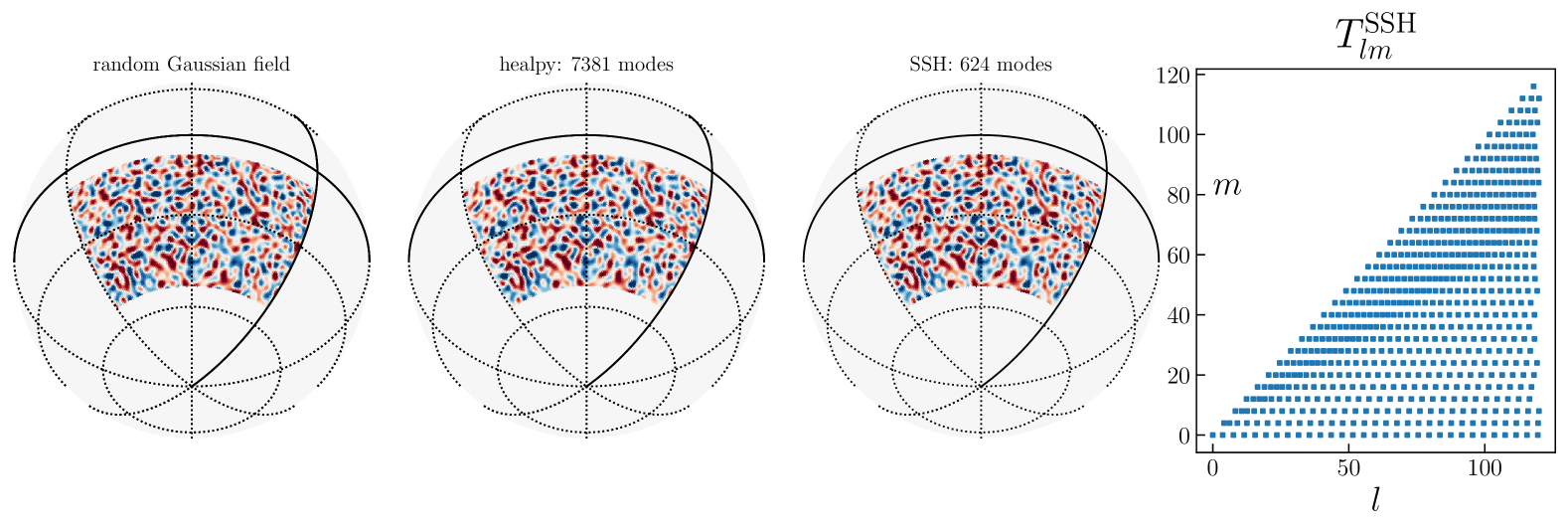
Figure 13: Spherical harmonic fitting with full-sky spherical harmonics (healpy) and spherical stripe harmonics (SSH). We show a realization of a random Gaussian field on the cut sky (left), which is then transformed to the $a_{lm}$ domain using the full-sky routines and the cut-sky SSH routines with an $l_{\rm max}=100$, and then transformed back into map-space. The full-sky routines use over 5000 modes for the given band-limit, while the SSH approach uses less then $5\times$ that amount. We show the sampling points in $lm$ space of the SSH modes (right), showing their sparsity and non-uniform sampling of harmonic space.

A.3 Polar Boundary Conditions

The polar component of the general solution is written up to a constant as $\Theta_{lm}(\theta)\propto P_{l}^{m}(\cos\theta)+\tilde{A}^{Q}_{lm}Q_{l}^{m}(\cos\theta)$. The standard conditions enforcing regularity for full-sky spherical harmonics are

$$\frac{d\Theta_{lm}(\theta^{\star})}{d\theta}=0\hskip 14.22636pt{\rm for}\ m =0$$ (43)

$$\Theta_{lm}(\theta^{\star})=0\hskip 14.22636pt{\rm for}\ m \neq 0,$$ (44)

where $\theta^{\star}$ is evaluated at the bounds of the interval at $\theta_{\rm min}=0$ and $\theta_{\rm max}=\pi$. For spherical cap harmonic formalism (Haines, 1985; ThéBault et al., 2006; Torta, 2019), we shift the maximum polar boundary to some arbitrary value within $0<\theta_{\rm max}<\pi$ and set a boundary condition on either the field or its derivative at the surface edge, also known as Dirichlet (Type 1) or Neumann (Type 2) conditions, respectively. This condition can be written as

$$C_{1}\Theta_{lm}(\theta_{\rm max})+C_{2}\Theta_{lm}^{\prime}(\theta_{\rm max})=0,$$ (45)

where one would set $C_{2}=0$ for Dirichlet conditions or $C_{1}=0$ for Neumann conditions, and $\Theta_{lm}^{\prime}$ is the polar derivative of $\Theta_{lm}$. The benefit of Neumann conditions is the ability to reconstruct an arbitrary signal amplitude when approaching the surface edge. Because $Q_{l}^{m}$ diverges at $\theta=0$ it is not included in the standard spherical harmonics or the spherical cap harmonics.

For the spherical stripe harmonics presented in this work, the boundary condition at $\theta_{\rm min}$ takes the same form as $\theta_{\rm max}$. However, in order to satisfy both boundary conditions we must now include $Q_{l}^{m}$ terms into the solution. Assuming, for simplicity but without loss of generality, Neumann conditions of $C_{1}=0$, the spherical stripe boundary conditions lead to the equality

$$P_{l}^{\prime m}(\cos\theta^{\star})+\tilde{A}_{lm}^{Q}Q_{l}^{\prime m}(\cos\theta^{\star})=0,$$ (46)

where $\theta^{\star}$ is evaluated at $\theta_{\rm min}$ and $\theta_{\rm max}$, and $P_{l}^{\prime m}$ is the polar derivative of $P_{l}^{m}$. This can be rearranged to form

$$\tilde{A}_{lm}^{Q}=\frac{-P_{l}^{\prime m}(\cos\theta^{\star})}{Q_{l}^{\prime m}(\cos\theta^{\star})},$$ (47)

where here $\cos\theta^{\star}$ can be evaluated at either $\theta_{\rm min}$ or $\theta_{\rm max}$, and

$$P_{l}^{\prime m}(\cos\theta_{\rm min})Q_{l}^{\prime m}(\cos\theta_{\rm max})-$$

$$P_{l}^{\prime m}(\cos\theta_{\rm max})Q_{l}^{\prime m}(\cos\theta_{\rm min})=0.$$ (48)

The latter is used to solve for the non-integer spectrum of $l$ for each integer $m$, and the former is used to solve for the $\tilde{A}_{lm}^{Q}$ coefficients for each $l$ and $m$. Normalization of the spherical harmonics $Y_{lm}(\theta,\phi)=\Theta_{lm}(\theta)\Phi_{m}(\phi)$ can then be performed such that their inner product sums to one.

Computing the associated Legendre functions $P_{l}^{m}(x)$ and $Q_{l}^{m}(x)$ on the interval $x\in[-1,1]$ for high orders ($l=m>100$) with standard formulas for the Gaussian hypergeometric function (Cohl & Costas-Santos, 2020) will result in numerical overflow even with double precision arithmetic. This is a result of the large dynamic range in the normalization factors that scale as $m!$ and $(l+m)!$, even though they effectivly cancel out in the final spherical harmonic. To alleviate this, one simply needs to scale down the hypergeometric function by $1/|m|!$ when computing it, and then re-normalize when applying the overall orthonormalization factor. Furthermore, evaluating factorial or gamma function products with large arguments in log space, summing and subtracting neighboring log factorials, and then exponentiating will help to prevent numerical overflow. In BayesLIM, these implementations allow for stable computation of high integer order and non-integer degree spherical harmonics up to $l=m\sim 400$, which is sufficiently high for the studies performed in this work.

A.4 Radial Boundary conditions

The general solution for the radial component is written up to a constant as $g_{l}(kr)\propto j_{l}(kr)+\tilde{A}^{y}_{l}y_{l}(kr)$. There are multiple methods for enacting boundary conditions along the radial dimension of the SFB, including imposing the field or its derivative go to zero at the boundary (e.g. Heavens & Taylor, 1995; Leistedt et al., 2012; Samushia, 2019; Chakraborty & Pullen, 2019), or imposing continuity on a potential field and its gradient (e.g. Fisher et al., 1995; Grasshorn Gebhardt & Doré, 2021). Doing so discretizes the $k$ wavevectors into a spectrum of $k_{n}$ orthogonal modes along the radial interval. Additionally, similar to the polar coordinate, we can choose to truncate the radial mask and enact the boundary conditions at an arbitrary $r_{\rm min}$ and $r_{\rm max}$. While many previous works have assumed the case of $r_{\rm min}\to 0$ for simplicity, recent studies have begun to derive boundary conditions for a non-trivial $r_{\rm min}$ (Samushia, 2019; Chakraborty & Pullen, 2019; Grasshorn Gebhardt & Doré, 2021).

For an intensity mapping survey with a well-defined radial selection function (i.e. the set of observed frequencies), it is fairly straightforward to take the latter approach. Imposing (Neumann) conditions at the radial boundaries yields

$$j_{l}^{\prime}(k_{ln}r^{\star})+\tilde{A}_{ln}^{y}y_{l}^{\prime}(k_{ln}r^{\star})=0,$$ (49)

where $r^{\star}$ is either $r_{\rm min}$ or $r_{\rm max}$. Similar to the polar axis case, we see that both the first and second order spherical Bessel functions are needed when using a non-vanishing $r_{\rm min}$. This yields the following equalities,

$$\tilde{A}_{ln}^{y}=\frac{-j_{l}^{\prime}(k_{ln}r^{\star})}{y_{l}^{\prime}(k_{ln}r^{\star})},$$ (50)

and

$$j_{l}^{\prime}(k_{ln}r_{\rm min})y_{l}^{\prime}(k_{ln}r_{\rm max})-j_{l}^{\prime}(k_{ln}r_{\rm max})y_{l}^{\prime}(k_{ln}r_{\rm min})=0.$$ (51)

The zeros of the latter equation yields the spectrum of $k_{ln}$ modes where our radial boundary conditions are satisfied, and the former can be used to compute the relative coefficient of the spherical Bessel functions. Finally, we can re-normalize the radial modes such that their inner products satisfy our previous orthogonality condition (Equation 39).

A.5 Power Spectrum Estimation

The 3D spatial Fourier transform of the temperature field is defined as

$$\widetilde{T}(\bm{k})=\int d^{3}r\ e^{i\bm{k}\bm{r}}T(\bm{r})$$ (52)

with its inverse transform defined as

$$T(\bm{r})=\int\frac{d^{3}k}{(2\pi)^{3}}\ e^{-i\bm{k}\bm{r}}\widetilde{T}(\bm{k}).$$ (53)

The relationship between the field in Fourier space and its power spectrum is

$$\langle\widetilde{T}(\bm{k})\widetilde{T}^{\ast}(\bm{k}^{\prime})\rangle=(2\pi)^{3}\delta^{D}(\bm{k}-\bm{k}^{\prime})P(\bm{k}),$$ (54)

where $\langle\rangle$ represents an ensemble average and $\delta^{D}(\bm{k}-\bm{k}^{\prime})$ is the Dirac delta function. To estimate the power spectrum with the SFB or SSFB formalism, we need a relation between $P(k)$ and the SFB coefficients of Equation 41, which is given in (Liu et al., 2016) as

$$\langle T_{lm}(k)T_{l^{\prime}m^{\prime}}^{\ast}(k^{\prime})\rangle=k^{-2}\delta^{D}(k-k^{\prime})\delta_{ll^{\prime}}\delta_{mm^{\prime}}P(k).$$ (55)

This demonstrates the close relationship between $\widetilde{T}(k)$ and $T_{lm}(k)$ modes and their connection to the power spectrum. This also shows us that the averaged, 1D power spectrum can be recovered by binning $T_{lm}(k)$ in $k$ and averaging over all $l$ and $m$ modes; however, (Liu et al., 2016) points out that for a practical survey, the minimum variance estimate of the power spectrum requires an $l$ (and possibly $m$) dependent weight in the average to account for the survey geometry.

To demonstrate the SSFB formalism in practice, we apply it here to a simulated wide-field 21 cm data cube using the quadratic estimator (QE) formalism (Hamilton, 1997; Tegmark, 1997; Liu et al., 2014; Dillon et al., 2015). For clarity, we will first briefly describe the quadratic estimator formalism: a full review is beyond the scope of this section and curious readers should consult the above references.

To make a numerical estimate of an underlying continuous power spectrum, we can discretize the power spectrum into a set of band powers. To do so, we model the continuous power spectrum as piecewise constant whose amplitudes in each $k$ band are called the band powers,

$$P(k)=p_{1}\Gamma_{1}(k)+p_{2}\Gamma_{2}(k)+\ldots=\sum_{\alpha}p_{\alpha}\Gamma_{\alpha}(k),$$ (56)

where $\Gamma_{\alpha}(k)$ is the windowing function of the $\alpha$ band power, which is 1 for all $k$ within $k_{\alpha}^{\rm min}<k<k_{\alpha}^{\rm max}$ and 0 otherwise. Notably, the band powers are linearly related to the covariance matrix of the data as

$$C(\bm{r},\bm{r}^{\prime})=\langle T(\bm{r})T(\bm{r}^{\prime})^{\ast}\rangle=\sum_{\alpha}p_{\alpha}C_{,\alpha}(\bm{r},\bm{r}^{\prime}),$$ (57)

where $C_{,\alpha}$ is the derivative of the covariance with respect to the $\alpha$ band power. If we discretize the temperature field (i.e. the data) into a column vector $\bm{x}$ of length $NM$ where $N$ is the number of radial shells and $M$ is the number of sky pixels, and discretize the SFB transform into a row vector $\bm{z}$ of the same size, we can express Equation 41 as

$$t_{lmn}=\bm{z}_{lmn}\bm{R}\bm{x},$$ (58)

where $\bm{z}_{lmn}$ is a row vector, $t_{lmn}$ is a single $T_{lm}(k_{n})$ coefficient, and $\bm{R}$ is a square matrix that acts as a pre-weighting of the data before taking the SFB transform. This can, for example, be a diagonal matrix that holds an apodization or windowing of the data such that the data transition smoothly to the mask boundaries. Throughout this section, we use lowercase boldface to denote vectors and uppercase boldface to denote matrices.

Drawing from our conclusion that the power spectrum is related to the square of $T_{lm}(k)$, we assert that an (unnormalized) estimate of the power spectrum can be written as

$$\hat{q}_{lmn}=t_{lmn}^{\ast}t_{lmn}=\bm{x}^{\dagger}\bm{R}^{\dagger}\bm{z}_{lmn}^{\dagger}\bm{z}_{lmn}\bm{R}\bm{x},$$ (59)

where $\hat{q}$ implies it is an estimate of $q$ from our finite survey volume. One may notice the similarity of Equation 59 to that of the quadratic estimator (Tegmark, 1997; Liu & Tegmark, 2011), where $\bm{z}_{lmn}^{\dagger}\bm{z}_{lmn}$ is equivalent to $C_{,\alpha}$ discussed before and $\alpha$ indexes a unique $lmn$ combination. We will use this similarity to derive certain statistical properties of the estimated power spectrum, specifically its window functions.

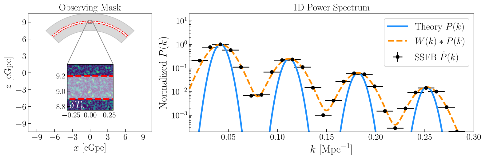
Figure 14: SSFB power spectrum recovery test of a simulated random Gaussian field. We show the azimuthal and radial extent of the observing mask (left), where $z$ is oriented along the line-of-sight, with a zoom-in inset showing the simulated random Gaussian field. We also show the recovered SSFB power spectrum (right) with their errorbars (black points), the theoretical input, double-tone power spectrum (blue), and the theoretically measured power spectrum (dashed orange), which is the theory $P(k)$ convolved with the SSFB estimator’s window function. The measured points are in good agreement with the convolved theory prediction, with small vertical errorbars given the large angular extent of the mask. We see accurate recovery of the location of the tones in $k$ space, as well as the relative amplitudes of the tones. All curves have been normalized by the peak of the theory curve (blue) to better capture the dynamic range as a function of $k$.

Following the quadratic estimator formalism, we introduce a normalization matrix $\bm{M}$ to produce a normalized estimate of the power spectrum,

$$\hat{p}_{\alpha}=\sum_{\beta}M_{\alpha\beta}\hat{q}_{\beta}.$$ (60)

Note that this does not show the usual bias term associated with the QE because we are assuming, for the sake of this demonstration, that the data is only populated by a signal term (no noise or foregrounds). Following Dillon et al. (2014), one can also ignore the bias terms if we use statistically independent samples for $\bm{x}$ in Equation 59, which is often the case in real analyses (HERA Collaboration et al., 2022). In case one isn’t using statistically independent noise draws, there will be a noise bias term, which can be estimated from the input noise covariance and subtracted.

Taking the expectation value of our estimated power spectrum yields

$$\langle\hat{p}_{\alpha}\rangle =\sum_{\alpha\beta}M_{\alpha\beta}\langle\hat{q}_{\beta}\rangle$$

$$=\sum_{\beta}M_{\alpha\beta}\operatorname{Tr}[\langle\bm{x}\bm{x}^{\dagger}\rangle\bm{R}^{\dagger}\bm{z}^{\dagger}_{\beta}\bm{z}_{\beta}\bm{R}]$$

$$=\sum_{\beta}M_{\alpha\beta}\sum_{\gamma}\operatorname{Tr}[\bm{z}^{\dagger}_{\gamma}\bm{z}_{\gamma}\bm{R}^{\dagger}\bm{z}^{\dagger}_{\beta}\bm{z}_{\beta}\bm{R}]p_{\gamma}$$

$$=\sum_{\beta\gamma}M_{\alpha\beta}|\bm{z}_{\beta}\bm{R}\bm{z}_{\gamma}^{\dagger}|^{2}p_{\gamma}$$

$$=\sum_{\beta\gamma}M_{\alpha\beta}H_{\beta\gamma}p_{\gamma},$$ (61)

where in the third line we used Equation 57, and in the fourth line we recognized that $\bm{z}_{\beta}\bm{R}\bm{z}_{\gamma}^{\dagger}$ is a scalar and $\bm{R}=\bm{R}^{\dagger}$. This final form reveals that the estimated bandpowers are related to the true bandpowers via a window function matrix $\bm{W}$ defined as

$$\langle\hat{\bm{p}}\rangle=\bm{M}\bm{H}\bm{p}=\bm{W}\bm{p}.$$ (62)

Various choices of the normalization matrix $\bm{M}$ can be made that yield different properties of the estimated bandpowers (e.g. Tegmark et al., 2002): the only constraint is that we choose an $\bm{M}$ matrix that allows the rows of $\bm{W}$ to sum to one, thus making $\hat{\bm{p}}$ an unbiased estimator (see also Liu & Tegmark, 2011; Liu et al., 2014; Dillon et al., 2015; Kern & Liu, 2021). In this work, we will adopt a diagonal $\bm{M}$ matrix that simply enforces this property for each row in $\bm{W}$.

Note that because of the orthogonality of $f_{lmn}$ with respect to $l^{\prime}$, $m^{\prime}$, and $n^{\prime}$ over the observing mask, one can show that the off-diagonal of $H_{\alpha\beta}$ vanish while the diagonal holds the inner product of $f_{lmn}$, making the window function also diagonal and therefore trivial. However, orthogonality is partially broken in the case a non-uniform pre-weighting $\bm{R}$ matrix. In this work, we apply a Hann tapering function across the line-of-sight axis, meaning the only non-trivial components of the window function are those of $\bm{W}_{n}^{n^{\prime}}$, which are considerably smaller and easier to compute than the general $\bm{W}_{lmn}^{l^{\prime}m^{\prime}n^{\prime}}$. This tapering (or apodization) is applied to reduce sidelobe $k$-mode ringing due to the fact that the real data do not strictly meet the boundary conditions assumed by the radial modes (either that the field or its derivative goes exactly to zero).

Next we demonstrate the ability of the SSFB approach to accurately model and re-construct a random Gaussian field observed through a spherical stripe observing mask, and ensure that it produces an accurate estimate of the field’s power spectrum. The mask used in this test extends across the azimuthal direction $-45^{\circ}<\phi<45^{\circ}$, the polar direction $35^{\circ}<\theta<80^{\circ}$, and the radial direction $8900<r<9200$ cMpc, which corresponds to a frequency range of 155–173 MHz and a redshift range of 7.2–8.2 for the 21 cm line. We simulate a 3D periodic box with $500^{3}$ voxels and a sidelength of $L=1000$ cMpc (2.0 cMpc resolution). The random field is drawn from a power spectrum with a decaying set of tones, with a maximum $k$ scale of 0.3 cMpc^-1. This test seeks to ensure that 1) the $k$ modes of the tones are recovered accurately and 2) the relative amplitude between the tones are recovered.

After generating a 3D Gaussian random field we tile it onto an NSIDE=512 HEALpix map at 64 different shells within the radial range. We do this by stacking the boxes in 3D out to the spherical shell comoving radius and use bilinear interpolation to sample each map pixel. We then band-limit the maps by smoothing them at an $l_{\max}=90$, and then downsample them to a NSIDE=128 HEALpix resolution. Note this is similar to how the 21 cm signal simulation is constructed in subsection 3.3.

The result of estimating the SSFB power spectrum on the simulations described above is shown in Figure 14, which shows a cut through the survey mask (left) where $z$ is oriented along the line-of-sight and the zoom-in inset shows the a slice of the simulated random Gaussian field. The gray shaded region shows the full extent of the volume probed by an experiment like HERA (50 - 250 MHz), while the red dashed box shows the region over which the power spectrum is actually estimated. The estimated spherical stripe Fourier Bessel (SSFB) power spectrum is plotted (right, dots) against the input quadruple-tone theory power spectrum (blue) and the theory power spectrum convolved with the SSFB estimator’s window function (dashed orange). Horizontal errorbars represent the full width half max of the window functions, vertical errorbars (not visible) represent sample variance on the signal given the finite volume. Relative to the convolved theory (dashed-orange), the SSFB estimator does a good job reconstructing the power spectrum, and accurately measures the location and relative amplitude of the inserted tones in the power spectrum. We artifically normalize the unitless power spectra by the peak theory curve (blue) to better capture the dynamic range as a function of $k$.

Appendix B Efficient Matrix-Vector Products for Dense Mass Matrices in HMC

Recall that the Hamiltonian Monte Carlo (HMC) approach to posterior sampling uses Hamiltonian dynamics to trace the trajectory of a particle in a potential well defined by the negative log posterior distribution (Neal, 2011). To briefly review our notation, we define the particle position and momentum column vectors as $\bm{q}$ and $\bm{p}$, respectively, where the position vector is a proxy for the forward model’s parameter vector. The covariance of the position vector is $\bm{C}$ and its inverse is called the mass matrix $\bm{M}$, which is equivalent to the model’s Hessian matrix (the matrix containing the posterior’s second derivatives with respect to the model parameters). We will define a lower-triangular Cholesky decomposition of the mass matrix as $\bm{M}=\bm{L}_{M}\bm{L}_{M}^{T}$. The key quantities that are required to accurately simulate this Hamiltonian trajectory are a series of matrix-vector products, including:

• $K=\tfrac{1}{2}\bm{p}^{T}\bm{M}^{-1}\bm{p}$ [kinetic energy term]

• $\partial_{t}\bm{q}=\bm{M}^{-1}\bm{p}$ [position update term]

• $\bm{p}=\bm{L}_{M}\bm{p}_{0}$ [momentum scaling term],

which can be found in Eqn. 2.6, Eqn. 2.7, and Sec. 4.1, respectively, from Neal (2011). In many cases, the mass matrix is approximated as diagonal, which simplifies the above matrix-vector products into trivial element-wise vector operations. However, for poorly conditioned posteriors this can make sampling extremely inefficient, and a dense mass matrix can dramatically improve sampling efficiency if such matrix operations can be computationally tolerated. However, even if we can compute and store the mass matrix, we generally will not want to invert it, as would be suggested by the above equations. General matrix inversion scales as $\mathcal{O}(N^{3})$ and can be unstable depending on the matrix’s condition number. Instead, we can use relationships between the previously defined Cholesky factors and use efficient triangular linear solves, which run in $\mathcal{O}(N^{2})$ time. Note that although Cholesky factorization also scales as $\mathcal{O}(N^{3})$ it has a smaller prefactor (roughly 3$\times$ faster than inversion), and is more stable than direct inversion (Nocedal & Wright, 2006).

One caveat is that the Hessian matrix may not necessarily be positive definite (e.g. if we are at a saddle point), which would prohibit a Cholesky factorization. To work around this, we can use the nearest positive definite approximation of the Hessian by regularizing it, which fits well with our Bayesian approach because this is equivalent to placing a stronger prior on our parameters. The total Hessian of the negative log posterior is simply the Hessian of the negative log likelihood summed with the Hessian of the negative log prior. To make the minimal adjustment needed to make the posterior Hessian symmetric positive definite (SPD), we experiment by adding small multiplicative increases to the computed prior Hessian until the posterior Hessian becomes SPD.

Next, given a permissible Cholesky factorization of the mass matrix, we will briefly show how we can compute the three required quantities for simulating HMC. First, we relate the inverse of the mass matrix to it’s Cholesky factors

$$\bm{M}^{-1}=\bm{L}_{M}^{-T}\bm{L}_{M}^{-1}.$$ (63)

Then, we can rewrite the kinetic energy term (1.) as

$$K=\tfrac{1}{2}(\bm{L}_{M}^{-1}\bm{p})^{T}\bm{L}_{M}^{-1}\bm{p}=\tfrac{1}{2}\bm{z}^{T}\bm{z}.$$ (64)

This means we can efficiently compute $\bm{z}$ via forward substitution of the linear system,

$$\bm{L}_{M}\bm{z}=\bm{p}.$$ (65)

Next, we can define a similar solution for the position update term (2.), which uses forward substitution followed by backward substitution. We can rewrite (2.) above as

$$\partial_{t}\bm{q}=\bm{M}^{-1}\bm{p}=\bm{L}_{M}^{-T}\bm{L}_{M}^{-1}\bm{p}=\bm{L}_{M}^{-T}\bm{z}.$$ (66)

We can first use forward substitution to solve $\bm{L}_{M}\bm{z}=\bm{p}$ for $\bm{z}$, then we can use backward substitution to solve $\bm{L}_{M}^{T}(\partial_{t}\bm{q})=\bm{z}$. Finally, computing (3.) is straightforward, where $\bm{p}_{0}\sim\mathcal{N}(0,1)$.

Relatedly, we can also draw uncorrelated samples from the parameter covariance $\bm{C}$ given only access to $\bm{L}_{M}$. To draw a random sample $\bm{v}\sim\mathcal{N}(0,\bm{C})$, usually we would first draw an uncorrelated unit-Gaussian vector $\bm{v}_{0}\sim\mathcal{N}(0,1)$ and then transform it by the Cholesky of the covariance. However, using the relationship above, we can also solve for $\bm{v}$ via backward substitution of

$$\bm{L}_{M}^{T}\bm{v}=\bm{v}_{0},$$ (67)

where $\bm{L}_{M}^{T}$ is upper triangular. Note that these are not draws from the true posterior, but are draws from a covariance defined implicitly by the mass matrix, which is an approximation to the true posterior (also known as the Laplace approximation).

We show the MCMC chains from our proof-of-concept run for a handful of parameters along with their averaged autocorrelations in Figure 8. Note that, as discussed in Appendix B, the HMC sampler is preconditioned with a block diagonal mass matrix, where each component in our data model (EoR, foreground, beam) is assumed to be dense, but the inter-component off-diagonals are zero (with the exception of the foreground-beam off-diagonals, which are kept for reasons discussed in subsection 4.2).

To assess how many independent samples we have drawn from the posterior we can compute the effective sample size (ESS). Because MCMC chains inevitably have some amount of correlation between samples, the effective sample size is generally less than the total sample size. The ESS is therefore defined as the chain length ($N$) divided by the average autocorrelation of the chain, computed as

$$N_{\rm eff}=\frac{N}{1+2\sum_{\tau=1}^{M}\rho(\tau)},$$ (68)

where $\rho(\tau)$ is the measured autocorrelation function of the chain as a function of the sample lag ($\tau$), and the sum runs up to an integer $M<N$ to limit sampling noise in $\rho(\tau)$ from affecting our $N_{\rm eff}$ estimate (Vehtari et al., 2021). For our MCMC chains shown in Figure 8, we compute the effective sample size by first taking the average of all measured autocorrelations functions within each component, and then use Equation 68 to derive $N_{\rm eff}$ for the averaged autocorrelation function (dashed lines in Figure 8). We compute effective sample sizes of 3, 5, & 15 for our EoR, foreground, & beam components, respectively, out of our $N\sim 500$ length chains. We suspect the beam component has a longer autocorrelation length because the underlying parameterization is more internally degenerate and more poorly conditioned than that of the foreground and EoR components.

One twist we added to make the sampling more efficient is an adaptive step size feature. Before sampling, we can tune the HMC step size to yield high acceptance probability, which we can do manually or automatically via a dual-averaging approach (Hoffman & Gelman, 2011). However, for complex distributions, for example ones that are not simply multivariate Gaussians, the sampler can walk into regions of parameter space with sufficiently higher curvature leading to larger HMC integration errors that force down the acceptance rate to very low levels. HMC step size adaptation is a means for trying to automatically adjust the step size to account for regions of higher curvature, such as the delayed rejection approach (Modi et al., 2024). Here, we use a similar but slightly different step size adjustment approach. Let the originally-tuned step size parameter be $\epsilon_{0}$. After simulating an HMC trajectory and evaluating the Metropolis-Hastings adjustment, if the acceptance probability falls below some pre-defined threshold (say 0.2) then we shrink the step size parameter by $\sim 20\%$ of its current value: in other words, we set $\epsilon\leftarrow\epsilon/1.2$. A new trajectory is then proposed and integrated and we repeat the update process, with a key difference being that the step size does not refresh to its original value, but keeps its reduced size. At the same time, for future trajectories, if the acceptance probability falls above the pre-defined threshold, we increase the step size by $\sim 20\%$ of its current value with a maximum achievable value of its original setting: in other words, $\epsilon\leftarrow{\rm Min}[\epsilon_{0},1.2\epsilon]$. Thus our approach can be thought of as a running step size adjustment that tracks the sampler as it walks through the parameter space. This is by no means an optimal step size adjustment procedure necessarily, but one that worked for the proof-of-concept at hand. Future work will aim to incorporate more complex and dynamic step size and mass matrix adaptations as needed.

Appendix C Computational Scaling

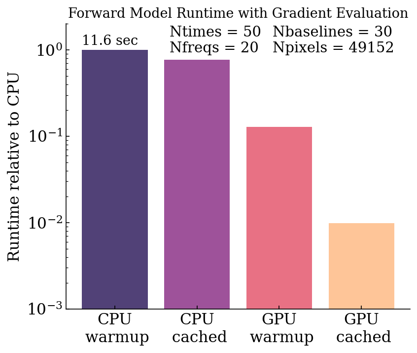
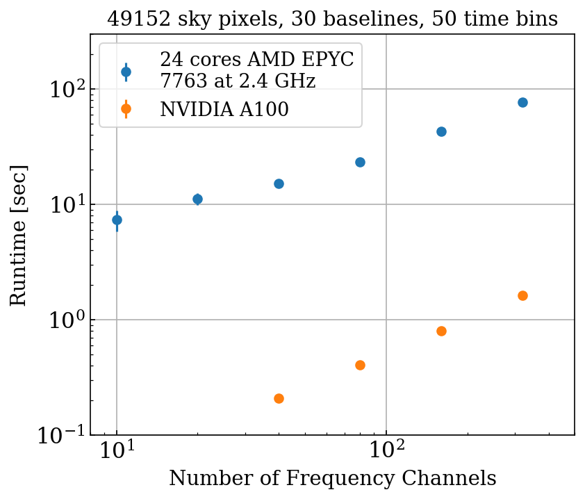
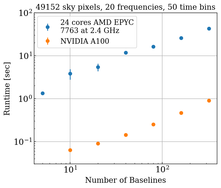
Figure 15: Computational benchmark and scaling tests of the BayesLIM forward model. The model used in these tests include an NSIDE 64 resolution sky map and a 1-degree resolution antenna primary beam model (hemispherical), where the parameters for each component are the pixel values. We simulate 20 frequency channels, 50 time bins, and 30 baseline vectors, and profile the total runtime of the foward pass and the backpropagation step. We run the profiling on a 24-core AMD EPYC 7763 CPU running at 2.4 GHz as well as a single NVIDIA A100 GPU. We find that roughly equal time is split between the forward pass and the backpropagation step. Left: The runtime of the model (forward pass and backpropagation step) on the CPU and GPU in a warm-up and a cached mode. Relative to the CPU timing, we see that the GPU in the cached mode delivers a factor of 100 in speed-up. Center: A scaling test showing the runtime in cached mode while varying the number of frequency channels. The plot the average and standard deviation of 20 runs for each scenario. We see the the runtime approach linear scaling. Right: A similar scaling test showing the runtime relative to the number of baselines in the data. Again we see similar speed-ups for the GPU relative to the CPU and linear scaling with an increased number of baselines.

Given the computational demands of the proposed framework, we run benchmarks and scaling tests to forecast the required computational load for an analysis on real data where the number of time stamps, frequencies, or baselines could be non-negligibly larger. In Figure 15 we show the results of CPU and GPU based benchmarks, as well as scaling tests while varying the number of frequency channels and baselines being computed. For the scaling tests, we plot the mean and standard deviation of 20 runs for each test case. The model adopted for these tests include a single NSIDE 64 resolution sky model ($t\times 10^{4}$ sky pixels), whose parameters are each sky pixel for each frequency channel, and a 1-degree resolution antenna primary beam model, whose parameters are each sky pixel for each frequency channel. We use a default of 30 baselines, 50 time bins, and 20 frequency channels, unless otherwise specified. The array model adopted is a HERA-217 array, but this is not actually relevant to the runtime of the tests, as what really matters is the number of unique baselines being simulated $(N_{\rm baselines}$), which is explicitly controlled for in the tests. Therefore, if we specify $N_{\rm baselines}=30$, this means we only simulate 30 baselines of the total number of unique baselines in the array, and the choice of baseline has no impact on the runtime. We run the profiling on 24 cores of a single AMD EPYC 7763 CPU clocked at 2.4 GHz, in addition to a single NVIDIA A100 GPU with 80 GB of VRAM. In both cases we run the model in double precision

We profile the runtime of a single gradient update, which involves the visibility simulation forward pass and the computation of the parameter gradients via backpropagation. For the model adopted here, roughly equal time is spent in the forward pass and the backward pass. For our first test (Left, Figure 15), we show the runtime on the CPU and the GPU in two modes. The first is a “warmup” mode where we have yet to compute intermediate products necessary for the forward pass (e.g. coordinate transformations, beam interpolation splines, etc.). These, it turns out, are often the bottleneck for realistic RIME visibility simulations Kittiwisit et al. (2025). The second mode, called a “cached” mode, is profiled where we cache all of these intermediate products so that they can be automatically resused. This allows the forward pass to be largely dominated by the matrix operations described by Equation 3, which allows the GPU to deliver significant acceleration. Thus, we see two orders of magnitude in speed-up delivered by the GPU relative to the CPU when operating in the cached mode (which is the normal operating mode after a single forward pass).

Next we show the results of model scaling with respect to the number of frequency channels and the number of simulated baselines (center and right, Figure 15). We plot the average and standard deviation of 20 runs for each test case. We expect to see asymptotic linear scaling with the number frequencies and baselines (Ewall-Wice et al., 2022; Kittiwisit et al., 2025), which we observe in both cases. For these tests we are always operating in the cached mode, and again observe a speed-up on the GPU by over an order of magnitude relative to the CPU. Assuming continued linear scaling, these benchmarks put BayesLIM on-par in terms of speed with other state-of-the-art, GPU-based visibility simulators that are being developed for next-generation radio telescopes like the SKA (Kittiwisit et al., 2025; O’Hara et al., 2025). Extrapolating these benchmarks to a realistic data quantity for HERA Phase II (Berkhout et al., 2024), we estimate that a similar analysis as demonstrated here but with double the the number of frequency channels and time integrations could be run in under a few hundred GPU hours, which is a very reasonable cost given the availability of GPU compute.

Memory limitations and CPU-to-GPU communications are often the bottlenecks when running a large model on a GPU. We can alleviate this by running the model in a data parallel manner, where we break the data into chunks and move it and an identical copy of the model over to a new GPU. After computing the gradient for that minibatch of data we can copy the gradient tensor back to a centralized GPU to be summed with the other workers, which is known as gradient accumulation. Assuming we have a fast GPU-to-GPU interconnect, this allows for near optimal parallelization across GPUs, in theory.

References

- Abbott et al. (2022) Abbott T. M. C., et al., 2022, Phys. Rev. D, 105, 023520
- Abdurashidova et al. (2022) Abdurashidova Z., et al., 2022, ApJ, 924, 51
- Aguirre et al. (2022) Aguirre J. E., et al., 2022, ApJ, 924, 85
- Alsing et al. (2023) Alsing J., Peiris H., Mortlock D., Leja J., Leistedt B., 2023, ApJS, 264, 29
- Amiri et al. (2024) Amiri M., et al., 2024, ApJ, 963, 23
- Anstey et al. (2021) Anstey D., de Lera Acedo E., Handley W., 2021, MNRAS, 506, 2041
- Anstey et al. (2023) Anstey D., de Lera Acedo E., Handley W., 2023, MNRAS, 520, 850
- Arfken & Weber (2005) Arfken G. B., Weber H. J., 2005, Mathematical methods for physicists 6th ed.
- Barry et al. (2019) Barry N., Beardsley A. P., Byrne R., Hazelton B., Morales M. F., Pober J. C., Sullivan I., 2019, Publ. Astron. Soc. Australia, 36, e026
- Bassett et al. (2021) Bassett N., Rapetti D., Tauscher K., Nhan B. D., Bordenave D. D., Hibbard J. J., Burns J. O., 2021, ApJ, 923, 33
- Berkhout et al. (2024) Berkhout L. M., et al., 2024, PASP, 136, 045002
- Bernardi et al. (2016) Bernardi G., et al., 2016, MNRAS, 461, 2847
- Betancourt (2017) Betancourt M., 2017, arXiv e-prints, p. arXiv:1701.02434
- BeyondPlanck Collaboration et al. (2023) BeyondPlanck Collaboration et al., 2023, A&A, 675, A1
- Binney & Quinn (1991) Binney J., Quinn T., 1991, MNRAS, 249, 678
- Böhm et al. (2021) Böhm V., Feng Y., Lee M. E., Dai B., 2021, Astronomy and Computing, 36, 100490
- Bowman et al. (2018) Bowman J. D., Rogers A. E. E., Monsalve R. A., Mozdzen T. J., Mahesh N., 2018, Nature, 555, 67
- Breitman et al. (2024) Breitman D., Mesinger A., Murray S. G., Prelogović D., Qin Y., Trotta R., 2024, MNRAS, 527, 9833
- Bull et al. (2015) Bull P., Ferreira P. G., Patel P., Santos M. G., 2015, ApJ, 803, 21
- Burba et al. (2023) Burba J., Sims P. H., Pober J. C., 2023, MNRAS, 520, 4443
- CHIME Collaboration et al. (2022) CHIME Collaboration et al., 2022, ApJS, 261, 29
- Campagne et al. (2023) Campagne J.-E., et al., 2023, The Open Journal of Astrophysics, 6, 15
- Carozzi & Woan (2009) Carozzi T. D., Woan G., 2009, MNRAS, 395, 1558
- Chakraborty & Pullen (2019) Chakraborty P., Pullen A. R., 2019, MNRAS, 488, 1828
- Chang et al. (2010) Chang T.-C., Pen U.-L., Bandura K., Peterson J., 2010, Nature, 466, 463
- Charles et al. (2023) Charles N., Kern N., Bernardi G., Bester L., Smirnov O., Fagnoni N., Acedo E. d. L., 2023, Monthly Notices of the Royal Astronomical Society, 522, 1009
- Cheng et al. (2024) Cheng Y.-T., Wang K., Wandelt B. D., Chang T.-C., Doré O., 2024, ApJ, 971, 159
- Cohen et al. (2007) Cohen A. S., Lane W. M., Cotton W. D., Kassim N. E., Lazio T. J. W., Perley R. A., Condon J. J., Erickson W. C., 2007, AJ, 134, 1245
- Cohl & Costas-Santos (2020) Cohl H. S., Costas-Santos R. S., 2020, Symmetry, 12
- Condon (1992) Condon J. J., 1992, ARA&A, 30, 575
- DESI Collaboration et al. (2024) DESI Collaboration et al., 2024, arXiv e-prints, p. arXiv:2411.12022
- Datta et al. (2010) Datta A., Bowman J., Carilli C., 2010, ApJ, 724, 526
- Davies et al. (2024) Davies F. B., et al., 2024, ApJ, 965, 134
- DeBoer et al. (2017) DeBoer D., et al., 2017, PASP, 129, 45001
- Dillon et al. (2014) Dillon J., et al., 2014, Phys. Rev. D, 89, 23002
- Dillon et al. (2015) Dillon J., et al., 2015, Phys. Rev. D, 91, 23002
- Dowell et al. (2017) Dowell J., Taylor G. B., Schinzel F. K., Kassim N. E., Stovall K., 2017, MNRAS, 469, 4537
- Duane et al. (1987) Duane S., Kennedy A., Pendleton B. J., Roweth D., 1987, Physics Letters B, 195, 216
- Eastwood et al. (2018) Eastwood M. W., et al., 2018, AJ, 156, 32
- Eriksen et al. (2004) Eriksen H. K., et al., 2004, ApJS, 155, 227
- Eriksen et al. (2008) Eriksen H. K., Jewell J. B., Dickinson C., Banday A. J., Górski K. M., Lawrence C. R., 2008, ApJ, 676, 10
- Ewall-Wice et al. (2020) Ewall-Wice A., et al., 2020, Monthly Notices of the Royal Astronomical Society, 500, 5195
- Ewall-Wice et al. (2022) Ewall-Wice A., Dillon J. S., Gehlot B., Parsons A., Cox T., Jacobs D. C., 2022, ApJ, 938, 151
- Fagnoni et al. (2020) Fagnoni N., et al., 2020, Monthly Notices of the Royal Astronomical Society, 500, 1232
- Fialkov et al. (2014) Fialkov A., Barkana R., Visbal E., 2014, Nature, 506, 197
- Fisher et al. (1995) Fisher K. B., Lahav O., Hoffman Y., Lynden-Bell D., Zaroubi S., 1995, MNRAS, 272, 885
- Fronenberg & Liu (2024) Fronenberg H., Liu A., 2024, ApJ, 975, 222
- Furlanetto et al. (2006) Furlanetto S., Oh S., Briggs F., 2006, Phys. Rep., 433, 181
- Garsden et al. (2024) Garsden H., et al., 2024, MNRAS, 535, 3218
- Girolami & Calderhead (2011) Girolami M., Calderhead B., 2011, Journal of the Royal Statistical Society: Series B (Statistical Methodology), 73, 123
- Glasscock et al. (2024) Glasscock K. A., Bull P., Burba J., Garsden H., Wilensky M. J., 2024, RAS Techniques and Instruments, 3, 607
- Górski et al. (2005) Górski K. M., Hivon E., Banday A. J., Wandelt B. D., Hansen F. K., Reinecke M., Bartelmann M., 2005, ApJ, 622, 759
- Grasshorn Gebhardt & Doré (2021) Grasshorn Gebhardt H. S., Doré O., 2021, arXiv e-prints, p. arXiv:2102.10079
- Gu et al. (2022) Gu A., et al., 2022, ApJ, 935, 49
- Gunes Baydin et al. (2015) Gunes Baydin A., Pearlmutter B. A., Andreyevich Radul A., Siskind J. M., 2015, arXiv e-prints, p. arXiv:1502.05767
- HERA Collaboration et al. (2022) HERA Collaboration et al., 2022, ApJ, 925, 221
- Hahn et al. (2023) Hahn C., et al., 2023, Proceedings of the National Academy of Science, 120, e2218810120
- Haines (1985) Haines G. V., 1985, Journal of Geophysical Research, 90, 2583
- Hamaker et al. (1996) Hamaker J. P., Bregman J. D., Sault R. J., 1996, A&AS, 117, 137
- Hamilton (1997) Hamilton A. J. S., 1997, MNRAS, 289, 285
- Haslam et al. (1982) Haslam C. G. T., Salter C. J., Stoffel H., Wilson W. E., 1982, A&AS, 47, 1
- Heavens & Taylor (1995) Heavens A. F., Taylor A. N., 1995, MNRAS, 275, 483
- Hernández-Sánchez et al. (2021) Hernández-Sánchez M., Kitaura F.-S., Ata M., Dalla Vecchia C., 2021, MNRAS, 502, 3976
- Hoffman & Gelman (2011) Hoffman M. D., Gelman A., 2011, arXiv e-prints, p. arXiv:1111.4246
- Horowitz et al. (2021) Horowitz B., Zhang B., Lee K.-G., Kooistra R., 2021, ApJ, 906, 110
- Hothi et al. (2020) Hothi I., et al., 2020, MNRAS,
- Hurley-Walker et al. (2017) Hurley-Walker N., et al., 2017, MNRAS, 464, 1146
- Hurley-Walker et al. (2022) Hurley-Walker N., et al., 2022, Publ. Astron. Soc. Australia, 39, e035
- Jasche & Wandelt (2013) Jasche J., Wandelt B. D., 2013, MNRAS, 432, 894
- Jelić et al. (2010) Jelić V., Zaroubi S., Labropoulos P., Bernardi G., de Bruyn A. G., Koopmans L. V. E., 2010, MNRAS, 409, 1647
- Jewell et al. (2004) Jewell J., Levin S., Anderson C. H., 2004, ApJ, 609, 1
- Josaitis et al. (2022) Josaitis A. T., Ewall-Wice A., Fagnoni N., Acedo E. d. L., 2022, MNRAS
- Kennedy et al. (2023) Kennedy F., Bull P., Wilensky M. J., Burba J., Choudhuri S., 2023, ApJS, 266, 23
- Kern & Liu (2021) Kern N. S., Liu A., 2021, MNRAS, 501, 1463
- Kern et al. (2019) Kern N. S., Parsons A. R., Dillon J. S., Lanman A. E., Fagnoni N., de Lera Acedo E., 2019, ApJ, 884, 105
- Kern et al. (2020a) Kern N. S., et al., 2020a, ApJ, 888, 70
- Kern et al. (2020b) Kern N. S., et al., 2020b, ApJ, 890, 122
- Kim et al. (2023) Kim H., et al., 2023, ApJ, 953, 136
- Kittiwisit et al. (2022) Kittiwisit P., Bowman J. D., Murray S. G., Gehlot B. K., Jacobs D. C., Beardsley A. P., 2022, MNRAS, 517, 2138
- Kittiwisit et al. (2025) Kittiwisit P., et al., 2025, RAS Techniques and Instruments, 4, rzaf001
- Kohn et al. (2016) Kohn S., et al., 2016, ApJ, 823, 88
- Kolopanis et al. (2019) Kolopanis M., et al., 2019, ApJ, 883, 133
- Kolopanis et al. (2023) Kolopanis M., Pober J. C., Jacobs D. C., McGraw S., 2023, MNRAS, 521, 5120
- Lanman & Kern (2019) Lanman A. E., Kern N., 2019, healvis: Radio interferometric visibility simulator based on HEALpix maps, Astrophysics Source Code Library (ascl:1907.002)
- Lanman et al. (2019) Lanman A., Hazelton B., Jacobs D., Kolopanis M., Pober J., Aguirre J., Thyagarajan N., 2019, The Journal of Open Source Software, 4, 1234
- Lanman et al. (2020) Lanman A. E., Pober J. C., Kern N. S., de Lera Acedo E., DeBoer D. R., Fagnoni N., 2020, MNRAS, 494, 3712
- Leistedt et al. (2012) Leistedt B., Rassat A., Réfrégier A., Starck J. L., 2012, A&A, 540, A60
- Li et al. (2024) Li Y., Modi C., Jamieson D., Zhang Y., Lu L., Feng Y., Lanusse F., Greengard L., 2024, ApJS, 270, 36
- Line (2022) Line J., 2022, The Journal of Open Source Software, 7, 3676
- Line et al. (2018) Line J. L. B., et al., 2018, Publ. Astron. Soc. Australia, 35, e045
- Line et al. (2020) Line J. L. B., et al., 2020, Publ. Astron. Soc. Australia, 37, e027
- Line et al. (2025) Line J. L. B., Trott C., Barry N., Null D., Jordan C. H., 2025, Publ. Astron. Soc. Australia, 42, e024
- Liu & Nocedal (1989) Liu D. C., Nocedal J., 1989, Mathematical Programming, 45, 503
- Liu & Shaw (2020) Liu A., Shaw J. R., 2020, PASP, 132, 062001
- Liu & Tegmark (2011) Liu A., Tegmark M., 2011, Phys. Rev. D, 83, 103006
- Liu et al. (2014) Liu A., Parsons A., Trott C., 2014, Phys. Rev. D, 90, 23018
- Liu et al. (2016) Liu A., Zhang Y., Parsons A., 2016, ApJ, 833, 242
- Loeb & Zaldarriaga (2004) Loeb A., Zaldarriaga M., 2004, Phys. Rev. Lett., 92, 211301
- Madau et al. (1997) Madau P., Meiksin A., Rees M., 1997, ApJ, 475, 429
- Mao et al. (2008) Mao Y., Tegmark M., McQuinn M., Zaldarriaga M., Zahn O., 2008, Phys. Rev. D, 78, 23529
- Mason et al. (2018) Mason C. A., Treu T., Dijkstra M., Mesinger A., Trenti M., Pentericci L., de Barros S., Vanzella E., 2018, ApJ, 856, 2
- Masui et al. (2013) Masui K. W., et al., 2013, ApJ, 763, L20
- McKinley et al. (2015) McKinley B., et al., 2015, MNRAS, 446, 3478
- Mertens et al. (2020) Mertens F. G., et al., 2020, MNRAS, 493, 1662
- Mertens et al. (2025) Mertens F. G., et al., 2025, arXiv e-prints, p. arXiv:2503.05576
- Mesinger et al. (2011) Mesinger A., Furlanetto S., Cen R., 2011, MNRAS, 411, 955
- Mesinger et al. (2012) Mesinger A., McQuinn M., Spergel D., 2012, MNRAS, 422, 1403
- Modi et al. (2024) Modi C., Barnett A., Carpenter B., 2024, Bayesian Analysis, 19, 815
- Moore et al. (2013) Moore D. F., Aguirre J. E., Parsons A. R., Jacobs D. C., Pober J. C., 2013, ApJ, 769, 154
- Morales & Hewitt (2004) Morales M. F., Hewitt J., 2004, ApJ, 615, 7
- Morales & Wyithe (2010) Morales M., Wyithe J., 2010, ARA&A, 48, 127
- Morales et al. (2012) Morales M., Hazelton B., Sullivan I., Beardsley A., 2012, ApJ, 752, 137
- Morales et al. (2019) Morales M. F., Beardsley A., Pober J., Barry N., Hazelton B., Jacobs D., Sullivan I., 2019, MNRAS, 483, 2207
- Mozdzen et al. (2019) Mozdzen T. J., Mahesh N., Monsalve R. A., Rogers A. E. E., Bowman J. D., 2019, MNRAS, 483, 4411
- Muñoz et al. (2024) Muñoz J. B., Mirocha J., Chisholm J., Furlanetto S. R., Mason C., 2024, MNRAS, 535, L37
- Munshi et al. (2024) Munshi S., et al., 2024, A&A, 681, A62
- Murphy et al. (2024) Murphy G. G., et al., 2024, MNRAS, 534, 2653
- Murray et al. (2022) Murray S. G., Bowman J. D., Sims P. H., Mahesh N., Rogers A. E. E., Monsalve R. A., Samson T., Vydula A. K., 2022, MNRAS, 517, 2264
- Neal (2011) Neal R., 2011, in , Handbook of Markov Chain Monte Carlo. pp 113–162, doi:10.1201/b10905
- Nocedal & Wright (2006) Nocedal J., Wright S. J., 2006, Numerical Optimization, second edn. Springer, New York, NY, USA
- Nunhokee et al. (2017) Nunhokee C. D., et al., 2017, ApJ, 848, 47
- Nunhokee et al. (2020) Nunhokee C. D., et al., 2020, ApJ, 897, 5
- O’Hara et al. (2025) O’Hara O. S. D., et al., 2025, MNRAS,
- Obuljen et al. (2018) Obuljen A., Castorina E., Villaescusa-Navarro F., Viel M., 2018, J. Cosmology Astropart. Phys., 2018, 004
- Paciga et al. (2013) Paciga G., et al., 2013, MNRAS, 433, 639
- Pagano et al. (2024) Pagano M., Sims P., Liu A., Anstey D., Handley W., de Lera Acedo E., 2024, MNRAS, 527, 5649
- Park et al. (2019) Park J., Mesinger A., Greig B., Gillet N., 2019, MNRAS, 484, 933
- Parsons et al. (2008) Parsons A., et al., 2008, PASP, 120, 1207
- Parsons et al. (2012) Parsons A., Pober J., Aguirre J., Carilli C., Jacobs D., Moore D., 2012, ApJ, 756, 165
- Parsons et al. (2016) Parsons A. R., Liu A., Ali Z. S., Cheng C., 2016, ApJ, 820, 51
- Paszke et al. (2019) Paszke A., et al., 2019, in Wallach H., Larochelle H., Beygelzimer A., d'Alché-Buc F., Fox E., Garnett R., eds, , Advances in Neural Information Processing Systems 32. Curran Associates, Inc., pp 8024–8035, http://papers.neurips.cc/paper/9015-pytorch-an-imperative-style-high-performance-deep-learning-library.pdf
- Paul et al. (2023) Paul S., Santos M. G., Chen Z., Wolz L., 2023, arXiv e-prints, p. arXiv:2301.11943
- Planck Collaboration et al. (2020) Planck Collaboration et al., 2020, A&A, 641, A6
- Pober et al. (2013) Pober J., et al., 2013, ApJ, 768, L36
- Pober et al. (2014) Pober J., et al., 2014, ApJ, 782, 66
- Pober et al. (2016) Pober J., et al., 2016, ApJ, 819, 8
- Popovic et al. (2023) Popovic B., Brout D., Kessler R., Scolnic D., 2023, ApJ, 945, 84
- Pratten & Munshi (2013) Pratten G., Munshi D., 2013, MNRAS, 436, 3792
- Prelogović & Mesinger (2024) Prelogović D., Mesinger A., 2024, A&A, 688, A199
- Price (2016) Price D. C., 2016, PyGDSM: Python interface to Global Diffuse Sky Models, Astrophysics Source Code Library, record ascl:1603.013
- Pritchard & Loeb (2012) Pritchard J., Loeb A., 2012, Reports Prog. Phys., 75, 86901
- Rapetti et al. (2020) Rapetti D., Tauscher K., Mirocha J., Burns J. O., 2020, ApJ, 897, 174
- Rassat & Refregier (2012) Rassat A., Refregier A., 2012, A&A, 540, A115
- Rath et al. (2024) Rath E., et al., 2024, arXiv e-prints, p. arXiv:2406.08549
- Remazeilles et al. (2015) Remazeilles M., Dickinson C., Banday A. J., Bigot-Sazy M. A., Ghosh T., 2015, MNRAS, 451, 4311
- Riseley et al. (2020) Riseley C. J., et al., 2020, Publ. Astron. Soc. Australia, 37, e029
- Robertson et al. (2015) Robertson B., Ellis R., Furlanetto S., Dunlop J., 2015, ApJ, 802, L19
- Robertson et al. (2023) Robertson B. E., et al., 2023, Nature Astronomy, 7, 611
- Samushia (2019) Samushia L., 2019, arXiv e-prints, p. arXiv:1906.05866
- Sault et al. (1996) Sault R. J., Hamaker J. P., Bregman J. D., 1996, A&AS, 117, 149
- Scheutwinkel et al. (2023) Scheutwinkel K. H., Handley W., de Lera Acedo E., 2023, Publ. Astron. Soc. Australia, 40, e016
- Scott & Rees (1990) Scott D., Rees M., 1990, MNRAS, 247, 510
- Shaw et al. (2014) Shaw J. R., Sigurdson K., Pen U.-L., Stebbins A., Sitwell M., 2014, ApJ, 781, 57
- Sims & Pober (2020) Sims P. H., Pober J. C., 2020, MNRAS, 492, 22
- Sims et al. (2019) Sims P. H., Lentati L., Pober J. C., Carilli C., Hobson M. P., Alexander P., Sutter P. M., 2019, MNRAS, 484, 4152
- Singh et al. (2018) Singh S., et al., 2018, ApJ, 858, 54
- Smirnov (2011) Smirnov O. M., 2011, A&A, 527, A106
- Sokolowski et al. (2017) Sokolowski M., et al., 2017, Publ. Astron. Soc. Australia, 34, e062
- Spinelli et al. (2021) Spinelli M., Bernardi G., Garsden H., Greenhill L. J., Fialkov A., Dowell J., Price D. C., 2021, MNRAS, 505, 1575
- Sullivan et al. (2012) Sullivan I. S., et al., 2012, ApJ, 759, 17
- Tan et al. (2021) Tan J., et al., 2021, ApJS, 255, 26
- Tauscher et al. (2018) Tauscher K., Rapetti D., Burns J. O., Switzer E., 2018, ApJ, 853, 187
- Tegmark (1997) Tegmark M., 1997, Phys. Rev. D, 55, 5895
- Tegmark et al. (2002) Tegmark M., Hamilton A. J. S., Xu Y., 2002, MNRAS, 335, 887
- The HERA Collaboration et al. (2022) The HERA Collaboration et al., 2022, arXiv e-prints, p. arXiv:2210.04912
- ThéBault et al. (2006) ThéBault E., Schott J. J., Mandea M., 2006, Journal of Geophysical Research (Solid Earth), 111, B01102
- Thyagarajan et al. (2015a) Thyagarajan N., et al., 2015a, ApJ, 804, 14
- Thyagarajan et al. (2015b) Thyagarajan N., et al., 2015b, ApJ, 807, L28
- Torta (2019) Torta J. M., 2019, Surveys in Geophysics, 41, 201
- Trott et al. (2012) Trott C., Wayth R., Tingay S., 2012, ApJ, 757, 101
- Trott et al. (2020) Trott C. M., et al., 2020, MNRAS, 493, 4711
- Vedantham et al. (2012) Vedantham H., Udaya Shankar N., Subrahmanyan R., 2012, ApJ, 745, 176
- Vehtari et al. (2021) Vehtari A., Gelman A., Simpson D., Carpenter B., Bürkner P.-C., 2021, Bayesian Analysis, 16, 667
- Wandelt et al. (2004) Wandelt B. D., Larson D. L., Lakshminarayanan A., 2004, Phys. Rev. D, 70, 083511
- Wilensky et al. (2023) Wilensky M. J., et al., 2023, MNRAS, 518, 6041
- Wilensky et al. (2024) Wilensky M. J., et al., 2024, RAS Techniques and Instruments, 3, 400
- Wilson et al. (2013) Wilson T. L., Rohlfs K., Hüttemeister S., 2013, Tools of Radio Astronomy, doi:10.1007/978-3-642-39950-3.
- Xu et al. (2024) Xu Z., et al., 2024, ApJ, 971, 16
- Yung et al. (2024) Yung L. Y. A., Somerville R. S., Finkelstein S. L., Wilkins S. M., Gardner J. P., 2024, MNRAS, 527, 5929
- Zeghal et al. (2022) Zeghal J., Lanusse F., Boucaud A., Remy B., Aubourg E., 2022, in Machine Learning for Astrophysics. p. 52 (arXiv:2207.05636), doi:10.48550/arXiv.2207.05636
- Zhang et al. (2016) Zhang L., Bunn E. F., Karakci A., Korotkov A., Sutter P. M., Timbie P. T., Tucker G. S., Wandelt B. D., 2016, ApJS, 222, 3
- Zheng et al. (2017) Zheng H., et al., 2017, MNRAS, 464, 3486
- Zonca et al. (2019) Zonca A., Singer L., Lenz D., Reinecke M., Rosset C., Hivon E., Gorski K., 2019, Journal of Open Source Software, 4, 1298
- de Oliveira-Costa et al. (2008) de Oliveira-Costa A., Tegmark M., Gaensler B. M., Jonas J., Landecker T. L., Reich P., 2008, MNRAS, 388, 247