Identifying Unknown Stochastic Dynamics via Finite expression methods

Abstract

Modeling stochastic differential equations (SDEs) is crucial for understanding complex dynamical systems in various scientific fields. Recent methods often employ neural network-based models, which typically represent SDEs through a combination of deterministic and stochastic terms. However, these models usually lack interpretability and have difficulty generalizing beyond their training domain. This paper introduces the Finite Expression Method (FEX), a symbolic learning approach designed to derive interpretable mathematical representations of the deterministic component of SDEs. For the stochastic component, we integrate FEX with advanced generative modeling techniques to provide a comprehensive representation of SDEs. The numerical experiments on linear, nonlinear, and multidimensional SDEs demonstrate that FEX generalizes well beyond the training domain and delivers more accurate long-term predictions compared to neural network-based methods. The symbolic expressions identified by FEX not only improve prediction accuracy but also offer valuable scientific insights into the underlying dynamics of the systems, paving the way for new scientific discoveries.

Key words. Stochastic differential equations, Symbolic learning, Generalization, Interpretability

1 Introduction

Stochastic differential equations (SDEs) are essential mathematical tools for modeling systems affected by random noise and uncertainty. They are widely applied in a variety of fields, including natural sciences and social systems [11]. Notable examples include particle motion in fluids and wind dynamics in physics, tumor growth in biology, and stock price fluctuations in finance [1, 24, 46, 6, 37]. Modeling SDEs from data is important for both the understanding and prediction of stochastic processes. To model SDEs from the data, one way is to solve the associated Fokker-Planck equation, which describes the time evolution of the probability density function of the system [21, 16]. Alternatively, one may aim to recover the drift and diffusion components directly. However, the inherent stochasticity of such systems makes learning an SDE challenging.

Advancements in data-driven computational methods have improved the ability to model SDEs. These approaches approximate unknown components of Itô-type SDEs by extracting patterns and mathematical structures from observational data. Gaussian processes provide nonparametric methods for capturing uncertainty in functional relationships, while polynomial approximations offer a simpler yet effective approach for systems with lower complexity. For more complex high-dimensional systems, advanced machine learning techniques such as deep neural networks [3, 36], generative adversarial networks [34, 38], and autoencoders [47] are employed to learn intricate patterns and latent structures within noisy data. These innovations enhance the ability to model and predict the behavior of systems driven by stochastic processes, even in cases where traditional analytical techniques struggle. Recently, a notable development has been the training-free conditional diffusion model [30], which uses the Monte Carlo method to approximate the exact closed-form score function without requiring neural network training. Using this approximated score function alongside labeled data generated from the corresponding reverse ODE, this approach facilitates supervised learning of the flow map in stochastic dynamics. These models mainly focus on producing numerical results rather than deriving explicit mathematical expressions, making it challenging to interpret the underlying learning process. This difficulty persists even for deterministic systems like ODE and becomes even more pronounced in the context of stochastic dynamics.

To overcome this limitation, symbolic learning has become a powerful tool for discovering governing equations, particularly through symbolic regression methods [9, 39, 42, 45]. These methods generally fall into two main categories. The first category focuses on exploring the solution space using techniques such as genetic programming and heuristic search [13, 19]. The second category leverages large-scale supervised pretraining, where models are trained on synthetic datasets to efficiently generate symbolic expressions [22, 27]. Beyond regression tasks, symbolic learning is also essential for deriving closed-form solutions for partial differential equations (PDEs). An approach to improving PDE solutions is symbolic regression based on genetic algorithms [2, 32], which incorporates automatic differentiation to refine the equations. More recently, Kolmogorov-Arnold Networks have been introduced in [31] to employ physics-regularized loss functions to enhance symbolic solutions and improve accuracy. Finite Expression Method (FEX) is a symbolic approach for high-dimensional problems, introduced in Refs. [28, 10, 20, 40]. FEX formulates the discovery of mathematical expressions as a combinatorial optimization (CO) problem. By integrating reinforcement learning (RL), it efficiently navigates a vast solution space, automating the identification of governing equations. This approach not only accelerates model development, but also ensures that the resulting expressions remain interpretable and aligned with underlying physical laws.

In this work, we assume that SDEs can be decomposed into deterministic and stochastic components, providing a structured framework for understanding complex dynamical systems. Our approach leverages the FEX method to learn the deterministic component, which is governed by underlying tendencies. Unlike conventional black-box models, FEX offers a transparent and interpretable framework that enables the discovery of unknown SDEs through explicit mathematical expressions for their evolution. To model the stochastic component, we incorporate advanced existing techniques, such as a variant of the training-free conditional diffusion model, as an example of methods that explicitly depend on latent random variables. Numerical experiments on various SDEs—including linear, nonlinear, and multidimensional systems—demonstrate the effectiveness of our approach. Additionally, our method remains highly flexible, allowing integration with other stochastic modeling techniques to ensure broad adaptability. By combining FEX with a model that accurately captures the stochastic component, our framework enables the separate extraction of drift and diffusion function while preserving accuracy, interpretability, and generalizability beyond the training domain. In addition, it ensures stability in long-term stochastic predictions. By integrating symbolic mathematical representations with deep learning, our approach bridges the gap between data-driven inference and traditional mathematical modeling, offering a more structured and interpretable framework for learning stochastic dynamics.

Compared with other methods in [4, 5, 30, 47, 48], this work introduces several key advantages:

• Explicit Mathematical Representation: Our approach provides a clear mathematical formulation for the deterministic component of unknown stochastic systems. This serves as a foundational benchmark for developing extended models and refining further stochastic components.

• Improved Generalization: By effectively capturing long-term stochastic behaviors, our framework maintains reliable performance. Unlike many data-driven models that struggle with extrapolation, our method continues to work well even beyond the training domain.

• Efficient Data Utilization: Leveraging explicit mathematical expressions, our framework requires significantly fewer trajectory data points than conventional learning-based approaches. This reduces computational costs while preserving accuracy, making it a more efficient alternative for modeling complex stochastic dynamics.

These advantages establish FEX as a powerful framework for modeling complex real-world systems, including those in finance, physics, and epidemiology, where governing equations are often unknown or difficult to analyze.

The remainder of this paper is organized as follows. Section 2 introduces the fundamental notations and concepts for learning SDEs from data. Section 3 presents an overview of FEX, followed by a detailed discussion on integrating a variant of the training-free diffusion model as an example in Section 4. Section 5 evaluates the performance of this approach through applications to analytical stochastic systems and real-world scenarios. Finally, the paper concludes with a summary in the last section.

2 Problem setting

Let $\left\{\Omega,\mathcal{F},\mathbb{P},\{\mathcal{F}_{t}\}_{0\leq t\leq T}\right\}$ be a complete filtered probability space supporting the Brownian motion $m-$ dimensional $W_{t}$. Here, $\{\mathcal{F}_{t}\}_{0\leq t\leq T}$ is the natural filtration of the Brownian motion $W_{t}$ augmented with the $\mathbb{P}$-null sets to ensure completeness.

2.1 Assumption

Within this probability space, we consider the following $d-$dimensional SDE:

(1) $$d\mathbf{x}_{t}=\mu(\mathbf{x}_{t})dt+\sigma(\mathbf{x}_{t})dW_{t},$$

where $\mu(\mathbf{x}_{t}):\mathbb{R}^{d}\to\mathbb{R}^{d}$, and $\sigma(\mathbf{x}_{t}):\mathbb{R}^{d}\to\mathbb{R}^{d\times m}$ with $m\in\mathbb{Z}_{+}$.

We impose the Lipschitz condition and the linear growth condition on $\mu(\mathbf{x}_{t})$ and $\sigma(\mathbf{x}_{t})$, ensuring the existence and uniqueness of the SDE solution. Moreover, we assume that both $\mu$ and $\sigma$ are time homogeneous, that is, they do not explicitly depend on time $t$, but only on the current state $\mathbf{x}_{t}$. Under these conditions, the solution takes the following form:

(2) $$\mathbf{x}_{t+\Delta t}=\mathbf{x}_{t}+\int_{t}^{t+\Delta t}\mu(\mathbf{x}_{s})\,ds+\int_{t}^{t+\Delta t}\sigma(\mathbf{x}_{s})\,dW_{s},$$

for any $0\leq t\leq T$ and $\Delta t>0$. Here, $\mathbf{x}_{t+\Delta t}$ represents the state of the process at time $t+\Delta t$, given that $\mathbf{x}_{t}$ at time $t$. The second term is an Itô integral, capturing stochastic fluctuations driven by Brownian motion $W_{t}$. Moreover, in this work, we assume $\mu$ and $\sigma$ are unknown, and that the Brownian motion $W_{t}$ is not observable.

2.2 Data Generation

In practice, solving (1) requires a numerical approximation. By discretizing time and approximating the integral form in (2), we can generate trajectories that capture the dynamics of the underlying stochastic system. To achieve this, we partition the time interval $[0,T]$ into discrete points:

$$\mathbf{\tau}=\left\{t_{n}|t_{n}=n\Delta t\quad\text{for}\quad n=0,1,...,N_{T}\right\},$$

where $N_{T}$ is the number of time steps, and the time increment is given by $\Delta t=T/N_{T}$. We assume that at least $N_{T}$ solution trajectories of $\mathbf{x}_{t}$ are observed at these discrete time points, using Euler-Maruyama (EM) discretization of (1), given by:

(3) $$\mathbf{x}_{t_{k+1}}=\mathbf{x}_{t_{k}}+\mu(\mathbf{x}_{t_{k}})\Delta t+\sigma(\mathbf{x}_{t_{k}})\Delta W_{t_{k}}\quad\text{for}\quad{k=0,1,...,N_{T}-1},$$

where $\Delta W_{t_{k}}$ represents the Brownian motion increment which is from Guassian distribution $\mathcal{N}(0,\Delta t)$. Thus, each trajectory consists of a sequence of observations:

(4) $$\mathbf{x}^{(j)}\left(t_{0}\right),\mathbf{x}^{(j)}\left(t_{1}\right),\ldots,\mathbf{x}^{(j)}\left(t_{N_{T}}\right),\quad j=1,\ldots,L,$$

where $L$ represents the number of trajectories. The initial state $\mathbf{x}^{(j)}\left(t_{0}\right)$ is sampled from a given initial distribution $p_{0}$. Under the assumption of time homogeneity, explicit time values are not necessary for modeling. Hence, we can represent the trajectory data as:

(5) $$\mathbf{x}^{(j)}_{0},\mathbf{x}^{(j)}_{1},\ldots,\mathbf{x}^{(j)}_{N_{T}},\quad j=1,\ldots,L,$$

which has the same format as equation (4) but without the need for notations of time variables. To construct the training dataset, we extract data pairs from each trajectory, leading to a total of $LN_{T}$ training samples which has the following form:

$$(\mathbf{x}_{0}^{(j)},\mathbf{x}_{1}^{(j)}),(\mathbf{x}_{1}^{(j)},\mathbf{x}_{2}^{(j)}),...,(\mathbf{x}_{N_{T}-1}^{(j)},\mathbf{x}_{N_{T}}^{(j)}),\quad j=1,...,L.$$

Since the stochastic process is time-homogeneous, we can regroup the data and further condense the dataset into the collection of paired observations:

(6) $$\mathscr{D}_{\text{obs}}=\left\{(\mathbf{X}_{0},\mathbf{X}_{1})\right\},$$

where $\mathbf{X}_{0}=\left[\mathbf{x}_{0}^{0},\mathbf{x}_{1}^{0},...,\mathbf{x}_{N_{T}-1}^{L}\right]^{T}\in\mathbb{R}^{N_{T}L\times d}$, and $\mathbf{X}_{1}=\left[\mathbf{x}_{1}^{0},\mathbf{x}_{2}^{0},...,\mathbf{x}_{N_{T}}^{L}\right]^{T}\in\mathbb{R}^{N_{T}L\times d}$.

2.3 Objective of this Work

To identify unknown SDEs, we assume that their dynamics can be decomposed into deterministic and stochastic components. The goal of this work is to develop a structured framework that learns these components separately from observed trajectory data. In each time step, we introduce a latent random variable $z_{k}\sim\mathcal{N}(0,I)$, which captures the sample-specific stochasticity. Based on this formulation, we can define a model $\mathbf{G}_{\theta}(x,z)$ , which reconstructs the underlying dynamics in alignment with (3):

(7) $$\bm{x}_{t_{k}+1} \approx\bm{x}_{t_{k}}+\mathbf{G}_{\theta}(\bm{x}_{t_{k}},z_{k}),$$

(8) $$\mathbf{G}_{\theta}(x,z) =\underbrace{\mathbf{D}_{\theta_{1}}(x)}_{\text{deterministic}}+\underbrace{\mathbf{S}_{\theta_{2}}(z)}_{\text{stochastic}}.$$

Here, $x$ denotes sample points from observed trajectories $\mathscr{D}_{\text{obs}}$, and $z$ is a latent variable drawn from a standard normal distribution. The model parameters $\theta=(\theta_{1},\theta_{2})$ jointly govern the deterministic and stochastic components of the dynamics. The function $\mathbf{D}_{\theta_{1}}(x)$ captures the underlying deterministic trends, while $\mathbf{S}_{\theta_{2}}(z)$ accounts for stochastic variability consistent with the diffusion term in the SDEs. This decomposition enables a structured and interpretable framework for learning stochastic dynamics from data.

In the next section, we will focus on using the observation dataset $\mathscr{D}_{\text{obs}}$ from (6) to derive the deterministic submap ${\mathbf{D}}_{\theta_{1}}(x)$. Using FEX, we aim to construct a fundamental mathematical representation of the deterministic component, establishing a foundation for further modeling the stochastic term.

3 Finite Expression Method (FEX) for deterministc component

In this section, we provide a detailed explanation of FEX to obtain $\mathbf{D}_{\theta_{1}}(x)$, which represents the deterministic component. Section 3.1 provides an overview of the fundamental concepts underlying FEX. Additionally, Section 3.2 expands on the computational rules that define expressions based on binary trees. Section 3.3 focuses on solving the CO problem, highlighting the reason for using $\mathbf{D}_{\theta_{1}}(x)$. To address the CO problem, we propose a systematic search loop that identifies effective operators capable of reconstructing the true solution when incorporated into an expression. More details on the CO problem and its resolution strategy are provided in the subsections of Section 3.3.

3.1 Description of FEX

FEX is a computational approach to solving differential equations by constructing closed-form expressions using a finite set of mathematical operators. Unlike traditional numerical methods and black-box machine learning models, FEX derives explicit analytical solutions within a structured function space, ensuring both interpretability and computational efficiency. This method has been successfully applied to solve PDE problems [28], dynamical systems [10], and various special problems [20, 40].

FEX represents expressions as a binary tree $\mathcal{T}$, where each node corresponds to a unary or a binary operation($u$ or $b$, respectively). The sets of unary operators and binary operators are denoted as $\mathbb{U}$ and $\mathbb{B}$, respectively. Thus, each expression is formed by an operator sequence $\mathbf{e}\in\mathbb{U}\cup\mathbb{B}$, with each operator linked to trainable parameters $\theta_{1}=\left\{\alpha,\beta\right\}$, where $\alpha$ represents a scaling parameter and $\beta$ is a bias term. This formulation allows the expression to be compactly represented as: $f(x,\mathcal{T},\mathbf{e},\theta_{1})$ with the input variable $x$.

3.2 Computational Rule of $\mathcal{T}$

The structure of a binary tree $\mathcal{T}$ is defined by several key components: the depth of the tree, denoted as $H$, determines the number of computational layers. Each input is represented as $i_{mn}$ where $m$ indicates the depth level and $n$ refers to the node index (specifically, when $n=1$, we denote $i_{mn}$ as $i_{m}$). The unary operators applied at a given depth are represented as $u_{mn}$, which corresponds to parameters $\alpha_{mn}$ and $\beta_{mn}$. Binary operators, denoted as $b_{mn}$, combine inputs based on their positions in the tree.

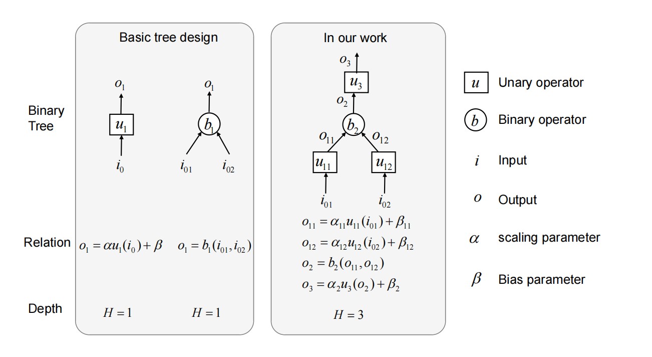
Fig. 1: The computational structure of a Basic tree and Binary tree in our work.

Figure 1 illustrates the binary tree structure at depths $H=1$ and $H=3$, which are utilized in our work. At depth $H=1$, a unary operator $u_{1}$ acts on a single input $i_{0}$, producing an output $o_{1}$. Alternatively, a binary operator $b_{1}$ can combine $i_{01}$ and $i_{02}$ to generate $o_{1}$. For depth $H=3$, unary operators $u_{11}$ and $u_{12}$ process inputs $i_{01}$ and $i_{02}$, respectively, resulting in intermediate outputs $o_{11}$ and $o_{12}$. These values are then combined by a binary operator $b_{2}$ to compute $o_{2}$, which undergoes a final unary transformation $u_{3}$ to produce $o_{3}$. This hierarchical design enhances the expressiveness of binary tree models, making them well-suited for complex function representation. For additional details on tree configurations, refer to [28].

3.3 Solving a CO in FEX

One of the key strengths of FEX is its ability to identify governing equations through an optimization framework that minimizes a functional loss $\mathcal{L}$ derived from (1). Using the results from (2), the functional $\mathcal{L}$ is defined as:

(9) $$\mathcal{L}(f)=\int_{\Omega}||\frac{\mathbf{x}_{t+\Delta t}-\mathbf{x}_{t}}{\Delta t}-f(\mathbf{x}_{t})||^{2}\rho(\mathbf{x}_{t})d\mathbf{x}_{t},$$

where $\rho$ is the probability density function of the observed data. To determine the optimal expression of drift tendency of SDE, we solve CO problem:

(10) $$\min\left\{\mathcal{L}(f(x,\mathcal{T},\mathbf{e},\theta_{1}))|\mathbf{e},\theta_{1}\text{ for a given $\mathcal{T}$}\right\}.$$

In practice, (9) and (10) can be reformulated into an empirical version, denoted as $\hat{\mathcal{L}}(f)$, using (6). This empirical loss is expressed as:

(11) $$\hat{\mathcal{L}}(f)=\frac{1}{N_{T}L}\sum_{i=1}^{N_{T}L}||\frac{\mathbf{X}_{1}^{(i)}-\mathbf{X}_{0}^{(i)}}{\Delta t}-f(\mathbf{X}_{0}^{i},\mathcal{T},\mathbf{e},\theta_{1})||^{2},$$

where $\mathbf{X}_{0}^{(i)}$ and $\mathbf{X}_{1}^{(i)}$ are the i-th state vectors sampled from $\mathbf{X}_{0}$ and $\mathbf{X}_{1}$ in (6), and it also leads to the optimization problem:

(12) $$\min\left\{\hat{\mathcal{L}}(f(\mathbf{X}_{0},\mathcal{T},\mathbf{e},\theta_{1}))|\mathbf{e},\theta_{1}\text{ for a given $\mathcal{T}$}\right\}.$$

FEX employs reinforcement learning techniques to explore the space of possible expressions, refining candidates iteratively based on their performance. This process in our work is illustrated in Figure 2 and involves key components such as score computations, operator selection, controller updates, and candidate refinement, which are discussed in the next subsection.

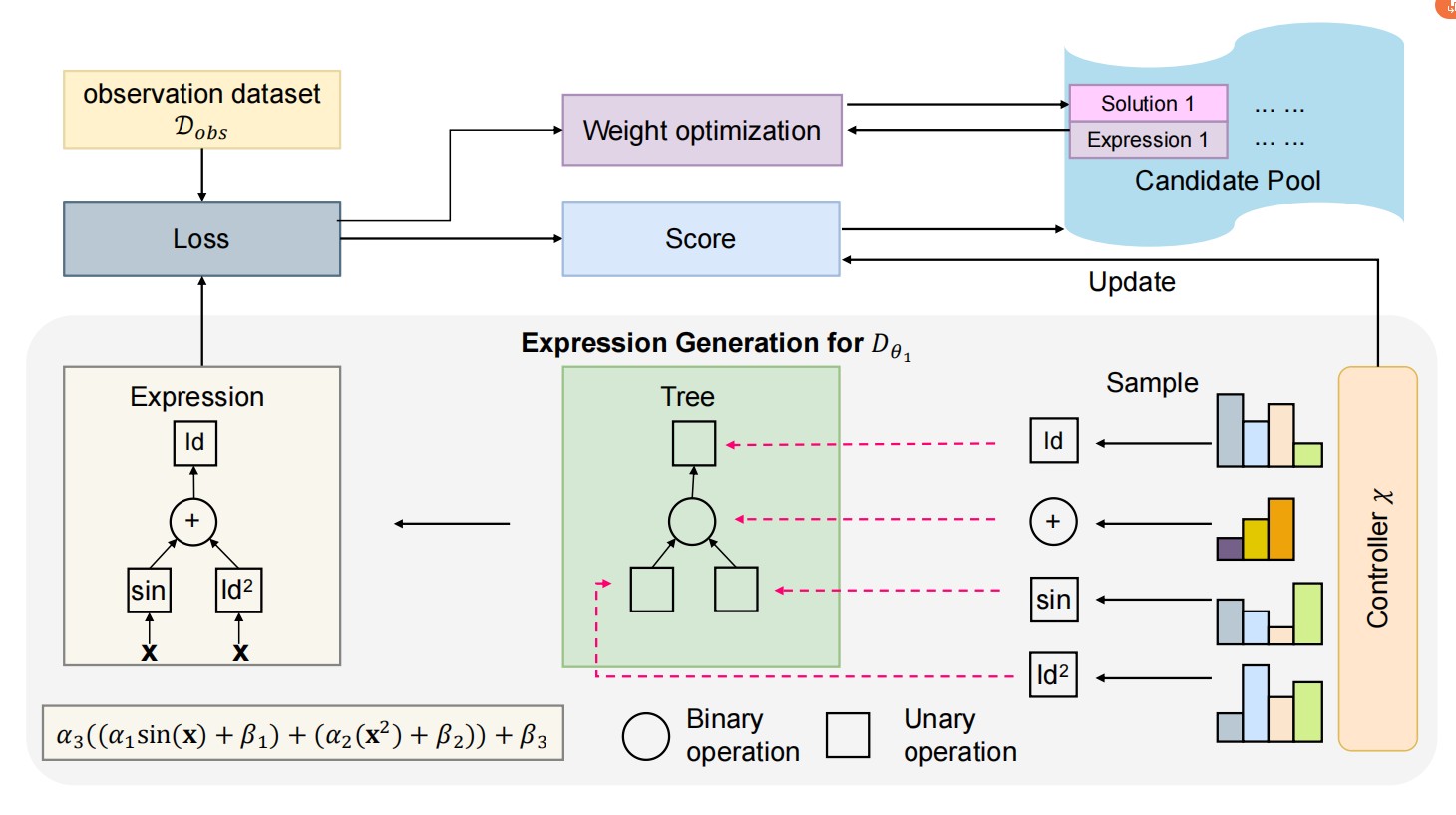
Fig. 2: Representation of a search loop of FEX implementation.

However, it is important to note that $f(x,\mathcal{T},\mathbf{e},\theta_{1})$ with the variable $x$ may not accurately represent the exact expression of the drift term. For practical purposes of our goal, the obtained expression serves as the deterministic component:

(13) $$\mathbf{D}_{\theta_{1}}(x)=f(x,\mathcal{T},\mathbf{e},\theta_{1}).$$

Remark 1.

If SDE in (1) follows a distribution other than Gaussian, such as an exponential distribution with expectation parameter $\lambda$, then (11) needs to be modified accordingly. Specifically, for an exponential distribution, we adjust the loss by subtracting $\lambda$ from the term inside the squared norm to correctly model the expected behavior of the data.

3.3.1 Score computation

The effectiveness of an operator sequence $\mathbf{e}$ is determined by a score function, which helps the controller prioritize optimal selections. This score is based on the ability of the sequences to minimize functional $\mathcal{L}$. We define the score of $\mathbf{e}$, $S(\mathbf{e})$, by

$$S(\mathbf{e})=\left(1+\sqrt{L(\mathbf{e})}\right)^{-1},\quad\text{where}\quad L(\mathbf{e})=\min_{\theta_{1}}\left\{\mathcal{L}(\hat{D}_{\theta_{1}}(\cdot))|\theta_{1}\right\}.$$

This ensures that sequences achieving lower losses receive higher scores, increasing their likelihood of being selected while reducing the influence of suboptimal choices.

3.3.2 Operator Sequence Generation

To ensure the proper generation of the operator sequence $\mathbf{e}$, we employ a robust control mechanism, the controller $\chi_{\Phi}$, which is parameterized by $\Phi$. This controller is designed to enhance the probability of selecting an operator sequence that aligns closely with the exact solution during the search loop in Figure 2. We represent the sampling process of $\mathbf{e}$ from the controller $\chi_{\Phi}$.

By treating the values of the tree nodes in $\mathcal{T}$ as random variables, the controller $\chi_{\Phi}$ generates probability mass functions $\mathbf{p}_{\Phi}^{1},\mathbf{p}_{\Phi}^{2},...,\mathbf{p}_{\Phi}^{s}$ to characterize their distributions, where $s$ is the total number of nodes. Each tree node value $e_{j}$ is sampled from $\mathbf{p}_{\Phi}^{j}$ to determine an operator. Consequently, the operator sequence $\mathbf{e}=(e_{1},e_{2},...,e_{s})$ is obtained as a sample from $\chi_{\Phi}$. In addition, we adopt the $\epsilon-$ greedy strategy [41] to improve the exploration of a potentially high score $\mathbf{e}$ which can potentially improve the quality of the search process.

3.3.3 Controller Update

In this work, the controller $\chi_{\Phi}$ is implemented using a neural network. The controller’s objective is to identify the operator sequence $\mathbf{e}$ that produces the highest score. Instead of optimizing the average scores of all generated operator sequences, following the method outlined in [35], we define the optimization problem as:

(14) $$\arg\max_{\Phi}\mathcal{J}(\Phi)=\arg\max\mathbb{E}_{\mathbf{e}\sim\chi_{\Phi}}\left\{S(\mathbf{e})|S(\mathbf{e})\geq S_{v,\Phi}\right\},$$

where $S_{v,\Phi}$ represents the $(1-v)\times 100\%$-quantile of the score distribution generated by $\chi_{\Phi}$. In practice, the model parameter $\Phi$ is updated via the gradient descent with a learning rate $\eta$ for

$$\Phi\leftarrow\Phi+\eta\nabla_{\Phi}\mathcal{J}(\Phi),$$

where $\nabla_{\Phi}\mathcal{J}(\Phi)\approx\frac{1}{N}\sum_{k=1}^{N}\left\{(S(\mathbf{e}^{(k)}))-\hat{S}_{v,\Phi})1_{S(\mathbf{e}^{(k)}))\geq\hat{S_{v},\Phi})}\sum_{i=1}^{s}\nabla_{\Phi}\log(\mathbf{p}_{\Phi}^{i}(\mathbf{e}_{i}^{k}))\right\}$ with $N$ is batch size, $\mathbf{e}^{(k)}$ represents the sampled operator sequence, and 1 is an indicator function that takes the value 1 if the condition inside holds and 0 otherwise. $\hat{S}_{v,\Phi}$ is the empirical $(1-v)-$ quantile of the observed score distribution.

3.3.4 Candidate Optimization

Note that the score of $\mathbf{e}$ is determined by optimizing a non-convex function $\mathcal{J}$ with random initialization, which can lead to local minima and a suboptimal solution. Consequently, the highest scoring sequence may not always correspond to the true solution. To mitigate this issue, we maintain a candidate pool $\mathbb{P}$ of size $N$ to store promising $\mathbf{e}$ of a high score.

During the search loop, if $\mathbb{P}$ has space available, newly generated sequences are added to $\mathbb{P}$ directly. When $\mathbb{P}$ reaches $N$, a new operator sequence can be added only if the score $S(\mathbf{e})$ is higher than the lowest score in the pool, while the lowest-ranked sequence is removed. This adaptive updating mechanism ensures that $\mathbb{P}$ retains the most promising candidates throughout optimization. Once the search loop is complete, the best sequences from $\mathbb{P}$, which we use to refine optimization (12) by adjusting hyperparameters and retraining to improve the likelihood of identifying an optimal solution, are obtained.

4 Existing methods for stochastic component

We now present the component of our framework that models the stochastic term in (7). Building upon the deterministic expression already defined, we can leverage advanced techniques to model the stochastic dynamics effectively. As an example, we introduce a score-based diffusion model that serves this purpose. Specifically, Section 4.1 presents the integration of this score-based model with the FEX framework, allowing the generation of labeled data for latent random variables via a Monte Carlo–approximated score function. Section 4.2 describes the training procedure for learning the stochastic submap $\mathbf{S}_{\theta_{2}}(z)$ using the generated data. Finally, Section 4.3 focuses on how to generate an effective drift term and diffusion term through $\mathbf{G}_{\theta}(x,z)$.

4.1 Training-free diffusion model

This method, originally proposed by [30], is integrated with the mathematical representation generated by FEX. We begin by defining the residual term $\mathbf{X}_{1}-\mathbf{X}_{0}-\Delta t\mathbf{D}_{\theta_{1}}(\mathbf{X}_{0})$ as $Z_{0}$, which is a random variable whose distribution depends on the underlying properties of $\mathbf{X}_{1}-\mathbf{X}_{0}$ and $\mathbf{D}_{\theta_{1}}(\mathbf{X}_{0})$. To model this randomness, we consider a forward linear SDE that progressively transforms $Z_{0}$ into a standard normal distribution:

(15) $$dZ_{\tau}=b(\tau)Z_{\tau}d\tau+\sigma(\tau)dW\tau\quad\text{with}\quad Z_{0}=\mathbf{X}_{1}-\mathbf{X}_{0}-\Delta t\mathbf{D}_{\theta_{1}}(\mathbf{X}_{0}),$$

where $\tau\in[0,1)$, $b(\tau)=\frac{d\log\alpha_{\tau}}{d\tau}$ and $\sigma^{2}(\tau)=\frac{d\beta^{2}_{\tau}}{d\tau}-2\frac{d\log\alpha_{\tau}}{d\tau}\beta_{\tau}^{2}$, with $\alpha_{\tau}=1-\tau$, $\beta^{2}=\tau$. The specific choice of coefficients ensures that the SDE transports the initial distribution $p_{Z_{0}}$ towards a standard normal distribution as $\tau\to 1$.

To corresponding reverse SDE, which generates new samples from the target distribution and act as a denoiser, is given by

(16) $$dZ_{\tau}=\left[b(\tau)Z_{\tau}-\sigma^{2}(\tau)S(Z_{\tau},\tau)\right]d\tau+\sigma(\tau)dB_{\tau}\quad\text{with}\quad Z_{1}=Z\sim\mathcal{N}(0,I_{d}),$$

where $B_{\tau}$ is the reverse-time Brownian motion and $S(Z_{\tau},\tau)$ is the score function defined as:

(17) $$S(Z_{\tau},\tau)=\nabla_{Z}\log p_{Z_{\tau}}(Z_{\tau}),$$

To further analyze the score, we consider its relation to PDF:

(18) $$\nabla p_{Z_{\tau}}(Z_{\tau})=p_{Z_{\tau}}(Z_{\tau})\nabla\log(p_{Z_{\tau}}(Z_{\tau}))=p_{Z_{\tau}}(Z_{\tau})S(Z_{\tau},\tau),$$

which holds true for all distribution of the exponential family. By considering the Fokker-Planck equation associated with (16), we obtain:

(19) $$\frac{\partial p_{Z_{\tau}}(Z_{\tau})}{\partial\tau}=\nabla\left[(b(\tau)Z_{\tau}-\sigma^{2}(\tau)S(Z_{\tau},\tau))p_{Z_{\tau}(Z_{\tau})}+\frac{\sigma^{2}(\tau)}{2}\nabla p_{Z_{\tau}}(Z_{\tau})\right].$$

By substituting (18) into (19), we obtain the reverse-time Fokker-Planck equation, which leads to the deterministic formulation as ordinary differential equation(ODE):

(20) $$dZ_{\tau}=\left[b(\tau)Z_{\tau}-\frac{1}{2}\sigma^{2}(\tau)S(Z_{\tau},\tau)\right]d\tau,$$

where $Z_{1}=Z\sim\mathcal{N}(0,I_{d})$, In practical applications, we discretize (20) using the Euler method to efficiently approximate the reverse process:

(21) $$Z_{\tau_{k-1}}=Z_{\tau_{k}}-\left[b(\tau_{k})Z_{\tau_{k}}-\frac{1}{2}\sigma^{2}(\tau_{k})S(Z_{\tau_{k}},\tau_{k})\right]\Delta{\tau},\quad k=K,...,1,$$

where $\Delta\tau=1/K$ and $\tau_{k}=k\Delta\tau$ for $k=0,1,...,K$. The choice of $K$ will be demonstrated in numerical experiments. Furthermore, to avoid training a neural network for score estimation, [30] introduces a Monte Carlo approximation of this score function which can be expressed as:

(22) $$\hat{S}(Z_{\tau_{k}},\tau_{k})\approx\frac{1}{N_{T}L}\sum_{i=1}^{N_{T}L}\frac{Z_{\tau_{k}}^{(i)}-\alpha_{\tau}Z_{0}^{(i)}}{\beta^{2}_{\tau_{k}}}\hat{w}(Z_{\tau_{k}}^{(i)},Z_{0}^{(i)}),$$

where $Z_{\tau_{k}}^{(i)}$ and $Z_{0}^{(i)}$ are $i-$ th component computed from observed data and $\hat{w}(Z_{\tau_{k}}^{(i)},Z_{0}^{(i)})$ are normalized weights reflecting likelihood contributions, defined as:

$$\hat{w}(Z_{\tau_{k}}^{(i)},Z_{0}^{(i)})=\frac{\exp\big{(}-\frac{||Z_{\tau_{k}}^{(i)}-\alpha_{\tau_{k}}Z_{0}^{(i)}||^{2}}{2\beta_{\tau_{k}}^{2}}\big{)}\exp\big{(}-\frac{||x-\mathbf{X}_{0}^{(i)}||^{2}}{2v^{2}}\big{)}}{\sum_{j=1}^{N_{T}L}\exp\big{(}\frac{||Z_{\tau_{k}}^{(j)}-\alpha_{\tau}Z_{0}^{(j)}||^{2}}{2\beta_{\tau_{k}}^{2}}\big{)}\exp\big{(}-\frac{||x-\mathbf{X}_{0}^{(j)}||^{2}}{2v^{2}}\big{)}}.$$

Note that we can apply $v=1$ when selecting the closest negligible number of scattering of trajectory data to accelerate the calculation for this score function numerically. Then we use (6), (21) and (22) to summarize the corresponding labeled dataset by:

(23) $$\mathscr{D}_{\text{label}}=\left\{(z_{j},y_{j})|z_{j}\sim\mathcal{N}(0,\mathbf{I}_{d}),y_{j}{\text{ is the numerical solution of (4.7), }j=1,...,J}\right\},$$

where for each $j$ can corresponds to a vector $Z_{0}^{(j)}$ which is gained from $Z_{0}$ through $\mathcal{D}_{\text{obs}}$ and $J$ is the size of the labeled dataset.

By incorporating discretized ODE data points, this method provides an interpretable mechanism for modeling the transformation of $Z_{0}$ and generates labeled data for supervised learning, ensuring accurate recovery of the stochastic component within the neural network framework described below.

4.2 Diffusion term Learning

Once $\mathscr{D}_{\text{label}}$ is generated, we train a fully connected neural network (FNN) to estimate the stochastic component $\mathbf{S}_{\theta_{2}}$ in (1). We may also define this neural network simply as $\mathbf{S}_{\theta_{2}}$. Mathematically speaking, given an activation function $\Phi$, let $M\in\mathbb{Z}_{+}$ denote the total number of layers, and let $W_{\mathrm{s}}\in\mathbb{Z}_{+}$ represent the width of the $\mathrm{s}$-th layer for $\mathrm{s}=1,...,M$. An FNN is modeled as a composition of $M$ simple nonlinear transformations:

(24) $$\hat{S}_{\theta_{2}}(z)=\mathbf{a}^{T}\mathbf{h}_{M}\circ\mathbf{h}_{M-1}\circ\cdots\mathbf{h}_{1}(z)\quad\text{for}\quad z\in\mathbb{R}^{d},$$

where $\mathbf{a}\in\mathbb{R}^{W_{M}}$; $\mathbf{h}_{\mathrm{s}}(z_{\mathrm{s}})=\Phi(\mathbf{W}_{\mathrm{s}}z_{\mathrm{s}}+\mathbf{b}_{\mathrm{s}})$ with $\mathbf{W}_{\mathrm{s}}\in\mathbb{R}^{W_{\mathrm{s}}\times W_{\mathrm{s}-1}}$; and $\mathbf{b}_{\mathrm{s}}\in\mathbb{R}^{W_{\mathrm{s}}}$. By a slight notational adjustment, $\Phi(z)$ means that $\Phi$ is applied entry-wise to a vector $z$ to obtain another vector of the same size. And $\theta_{2}=\left\{\mathbf{a},\mathbf{W}_{\mathrm{s}},\mathbf{b}_{\mathrm{s}}:1\leq\mathrm{s}\leq M\right\}$ is the set of all parameters to determine the underlying neural network. To ensure flexibility and expressive power, common activation functions such as the ReLU and the tanh function are used. Here, the network is trained using MSE loss between the predicted outputs and the labeled dataset. Given input samples $z_{j}$, we optimize ${\theta_{2}}$ by using the following objective function:

(25) $$\theta_{2}^{*}=\arg\min_{\theta_{2}}\frac{1}{J}||\mathbf{S}_{\theta_{2}}(z_{j})-y_{j}||_{2}^{2}.$$

Once the optimal parameters $\theta_{2}^{*}$ are obtained and applied to $\hat{S}_{\theta_{2}}$, the diffusion term is learned not only for the pointwise estimation but also for the distribution-level modeling, ensuring a more accurate representation of the stochastic process.

4.3 Generating efficient drift and diffusion terms

To examine the accuracy of our framework, we propose the following estimator as efficient drift and diffusion terms:

Let $\mathbf{Z_{j}}$ be the random variables sampled from standard normal distribution corresponding to $\mathbf{X}_{0}$ through (15). The refined estimator for the drift term is:

(26) $$\hat{\mu}(\mathbf{X}_{0})=\frac{1}{N_{T}L}\sum_{i=1}^{N_{T}L}\left[\mathbf{S}_{\theta_{2}}(\mathbf{Z}^{(i)})+\mathbf{X}_{0}^{(i)}+\Delta t\mathbf{D}_{\theta_{1}}(\mathbf{X}_{0}^{i})\right].$$

Similarly, the stochastic component is refined as

(27) $$\hat{\sigma}(\mathbf{X}_{0})=\text{Std}(\left[\mathbf{S}_{\theta_{2}}(\mathbf{Z})+\mathbf{X}_{0}+\Delta t\mathbf{D}_{\theta_{1}}(\mathbf{X}_{0})\right]).$$

With these refinements, we recover the effective drift and diffusion terms through the framework defined in (7). The complete workflow of the proposed method is summarized in the following algorithm. Although alternative models can also be used to identify the stochastic component, the FEX-based formulation provides a distinctive approach, enabling different treatments and yielding refined versions of the drift and diffusion terms tailored to this framework.

Algorithm 1 A training free diffusion model govern by FEX

Input: Observation dataset $\mathcal{D}_{\text{obs}}=\{(\mathbf{X}_{0}^{(i)},\mathbf{X}_{1}^{(i)})\}_{i=1}^{N_{T}L}$
Output: The model $\mathbf{G}_{\theta}(x,z)$

1:Procedure:

2:Train FEX term $\mathbf{D}_{\theta_{1}}(x)$ using $\mathcal{D}_{\text{obs}}$;$\triangleright$ Generating approximated term

3:Compute the term $Z_{0}=\mathbf{X}_{1}-\mathbf{X}_{0}-\Delta t\mathbf{D}_{\theta_{1}}(\mathbf{X}_{0})$;

4:for $j=1,2,\dots,J$ do $\triangleright$ Generating labeled data

5:  Randomly select a sample $Z_{0j}$ from $Z_{0}$;

6:  Generate a sample $z_{j}$ from $\mathcal{N}(0,\mathbf{I}_{d})$ and set $Z_{\tau_{K}}=z_{j}$ in (21);

7:  for $k=K,\dots,1$ do

8:   Compute the score function $\hat{S}(Z_{\tau_{k}},\tau_{k})$ mentioned in [30];

9:   Solve $Z_{\tau_{k-1}}$ using the Euler scheme in (21);

10:  end for

11:  Set $y_{j}=Z_{\tau_{0}}$ and assemble dataset $(z_{j},y_{j})$ which corresponds to $Z_{0}^{(j)}$;

12:end for

13:Train $\mathbf{S}_{\theta_{2}}(z)$ using the labeled dataset $\mathcal{D}_{\text{label}}=\{(z_{j},y_{j})\}_{j=1}^{J}$;

14:Obtain $G_{\theta}(x,z)$ then deduce $\hat{\mu}(x)$ and $\hat{\sigma}(x)$;

5 Numerical Experiments

In this section, we conduct a series of numerical experiments to evaluate the effectiveness of the FEX applied to learning stochastic dynamical systems. The selected examples encompass a diverse range of SDEs, including

• Linear SDEs: We consider only Ornstein–Uhlenbeck (OU) Process, which serves as a key example due to its well-characterized steady-state distribution and its widespread application in modeling noise-driven dynamics. It also describes a system that undergoes random fluctuations while exhibiting a tendency to revert to a long-term mean. Originally introduced by Uhlenbeck and Ornstein in the context of Brownian motion [43], this process has been widely applied in various fields, including finance [44], biology [14], and statistical physics [12].

• Nonlinear SDEs: To assess the capability of FEX in handling more complex, nonlinear stochastic dynamics, we consider three distinct nonlinear SDEs:

  • SDE with Trigonometric Drift Functions: These SDEs are designed to model periodic stochastic dynamics commonly observed in biological rhythms, climate systems, and fluid dynamics. Incorporating trigonometric terms introduces oscillatory behavior, which is essential to capture cyclic phenomena in nature [23, 33].

  • Double-well Potential Model: This class of SDEs describes metastable dynamics, where a system fluctuates between two potential wells under stochastic influences. Such models are widely used in chemical reaction kinetics, statistical mechanics, and phase-transition dynamics. Building on Kramers reaction rate theory [26], they provide a theoretical foundation for understanding bi-stability and noise-induced transitions [17].

  • Oscillatory Langevin (OL) Process: The OL process generalizes the classical Langevin equation by incorporating inertia-driven oscillations alongside stochastic fluctuations. Unlike standard mean-reverting processes, this model accounts for both damping and oscillatory effects, making it particularly relevant in molecular dynamics, soft matter physics, and nonequilibrium thermodynamics [15, 7]. It serves as a crucial framework for studying systems that exhibit stochastic resonance, active matter dynamics, and energy dissipation in fluctuating environments.

• SDEs with Non-Gaussian Noise: SDEs driven by non-Gaussian noise provide a powerful framework for modeling systems characterized by irregular and discontinuous fluctuations. Unlike traditional Gaussian noise, which assumes normally distributed variations, exponentially distributed noise and other heavy-tailed processes play a crucial role in capturing asymmetric, skewed, and jump-like behaviors. These types of SDEs are particularly prevalent in fields such as financial markets, where asset price movements often exhibit sudden jumps [8], ecological dynamics, where environmental disturbances follow non-Gaussian distributions [25], and neuroscience, where synaptic input and neural spiking can be irregular and burst-like [29].

The Construction of Training Dataset

For each case, we generate trajectory datasets of varying sizes by numerical integration (1) using the Euler-Maruyama method. The number of trajectories varies by scenario, with some cases producing up to 10,000 trajectories, as an example. Then this results in observation data $\mathcal{D}_{\text{obs}}$ of size $100,000$ for $N_{T}L$. The initial conditions are uniformly sampled from predefined regions specific to each case. Simulations are performed using a fixed time step of $\Delta t=0.01$ over a total time horizon of $T=1.0$.

Implementation of FEX

The FEX framework is designed to construct and optimize mathematical expressions using a binary tree structure, a neural network-based controller, and an adaptive score computing mechanism. In the following, we highlight four essential components of its implementation.

• For computation, the score is optimized using the Adam algorithm with an initial learning rate $8.0\times 10^{-3}$ for $10,000$ iterations. The loss function (11) guides this optimization process.

• The binary tree, consisting of three unary operators and one binary operator, is used to construct mathematical expressions, as shown in Figure 1. The binary operator set is defined as $\mathbb{B}=\{+,-,\times\}$, while the unary operator set is given by:

  $$\mathbb{U}=\{\sin(x),\cos(x),\exp(x),0,1,x,x^{2},x^{3},x^{4}\},$$

  where $x$ represents the variable.

• An FNN is used as a controller $\chi_{\Phi}$ with constant input. The output size of the controller NN is determined by $|\mathbb{B}|+3|\mathbb{U}|$ representing the number of binary and unary operators, respectively, and $|\cdot|$ denotes the cardinality of a set. For controller updates, the policy gradient method is used with a batch size of 2. The controller is trained using the Adam optimizer with a fixed learning rate of 0.002, while the number of training iterations is adjusted according to the specific case requirements.

• Due to potential ambiguities in the selection of expressions, the capacity of the candidate pool is set to $N=30$, ensuring robustness in the identification of expressions that align with the ground truth while minimizing the potential interference with the diffusion term in Equation (1). For any $\mathbf{e}\in\mathbb{P}$, parameter optimization is performed using the Adam optimizer, starting with an initial learning rate of $0.005$ for $80,000$ iterations. The learning rate is gradually reduced following a cosine decay schedule [18] to improve stability and convergence.

Settings for $\mathbf{S}_{\theta_{2}}(z)$

For each case, we randomly select clustered points from the observation dataset, which serves to calculate the Monte Carlo approximation of the score function. The reverse-time ODE is then solved with $K=10,000$, producing the labeled dataset $\mathcal{D}_{\text{label}}$. To train $\mathbf{S}_{\theta_{2}}(z)$, we divide $\mathcal{D}_{\text{label}}$ into training sets $80\%$ and validation sets $20\%$, used exclusively for FNN which consists of a single hidden layer with 50 neurons and employs the tanh activation function. Each experiment trains the FNN for 2000 epochs using the Adam optimizer, with a learning rate of $0.01$ and a weight decay of $10^{-6}$ to mitigate overfitting.

Evaluation Metrics for Testing $\mathbf{G}_{\theta}(x;z)$

This framework is evaluated based on its ability to predict SDE over an extended time horizon for $T=5$ with the flexibility to perform a detailed evaluation of long-term predictive performance. For all numerical experiments, we simulate $500,000$ trajectories in 1-dimensional cases and $10,000$ trajectories in 2-dimensional cases using both $\mathbf{G}_{\theta}(x;z)$ and the ground truth, then compare their outputs based on the following criteria:

• Statistical Robustness: The mean and standard deviation of the simulated trajectories are analyzed to assess their alignment with the expected distribution, confirming that the model maintains consistency in the broader domain.

• Drift and diffusion accuracy: The estimated drift and diffusion coefficients of the simulated trajectories are compared against the true drift and diffusion values, even in some regions beyond the training domain.

By evaluating performance over a broader, previously unseen domain, we assess how well this framework can generalize beyond the observed data, highlighting its potential for application to more complex stochastic systems. In the following figures, FEX-TF-DM refers to a training-free diffusion model governed by FEX, while TF-CDM denotes a training-free conditional diffusion model, as introduced in [30].

5.1 Linear SDEs

We first consider two cases for the OU process in different dimensions.

5.1.1 1-dimensional OU process

The evolution of the one-dimensional OU process is governed by the following SDE:

(28) $$d\mathbf{x}_{t}=\theta(\mu-\mathbf{x}_{t})dt+\sigma dW_{t},$$

where $\theta=1.0,\mu=1.2$ and $\sigma=0.3$. The observation dataset $\mathcal{D}_{obs}$ is constructed by generating $L=15,000$ trajectories samples, obtained by solving (28) with initial values drawn uniformly from $U(0,2.5)$ up to $T=1.0$. To estimate the deterministic component $\mathbf{D}_{\theta_{1}}(\mathbf{x}_{t})$, we randomly select 50,000 initial states from $\mathcal{D}_{\text{obs}}$ and apply the principles discussed in Section 3 to derive an analytic representation, as presented in Table 1.

True drift expression	Best expression for $\mathbf{D}_{\theta_{1}}(\mathbf{x}_{t})$
$1.2-\mathbf{x}_{t}$	$1.1989-0.9953\mathbf{x}_{t}$

Table 1: Comparison of true drift term and the FEX-learned deterministic component.

The model indicated by $\mathbf{G}_{\theta}$ is evaluated against the true solution, as shown in Figure 3, using four different initial conditions $\mathbf{x}_{0}=-6,1.5,6$, respectively. In particular, $\mathbf{x}_{0}=-6$ and $6$ are outside the range of the training domain $(0,2.5)$. Despite this, the proposed approach maintains high fidelity to the true solution trajectory up to $T=5.0$, showcasing excellent extrapolation ability far beyond the training horizon of $T=1.0$, outperforming previous techniques such as the one described in [30]. Figure 4 illustrates the learned one-step conditional distributions, which are visually consistent with the true distributions for all initial conditions tested, confirming the effectiveness of the model in accurately characterizing the underlying stochastic dynamics.

In addition, Figure 5 presents the effective estimators $\hat{\mu}$ and $\hat{\sigma}$ compared to their true counterparts in a broader domain of $[-6,6]$, which extends well beyond the training interval. The model accurately identifies the drift and diffusion functions and demonstrates strong generalization performance across this extended range. This behavior indicates that the model captures the essential structure of the dynamics and maintains reliable predictions even at extrapolated values. The relative errors for both the drift and diffusion functions remain low, approximately on the order of $10^{-2}$ and $10^{-3}$, respectively, further demonstrating the robustness of the model $\mathbf{G}_{\theta}$.

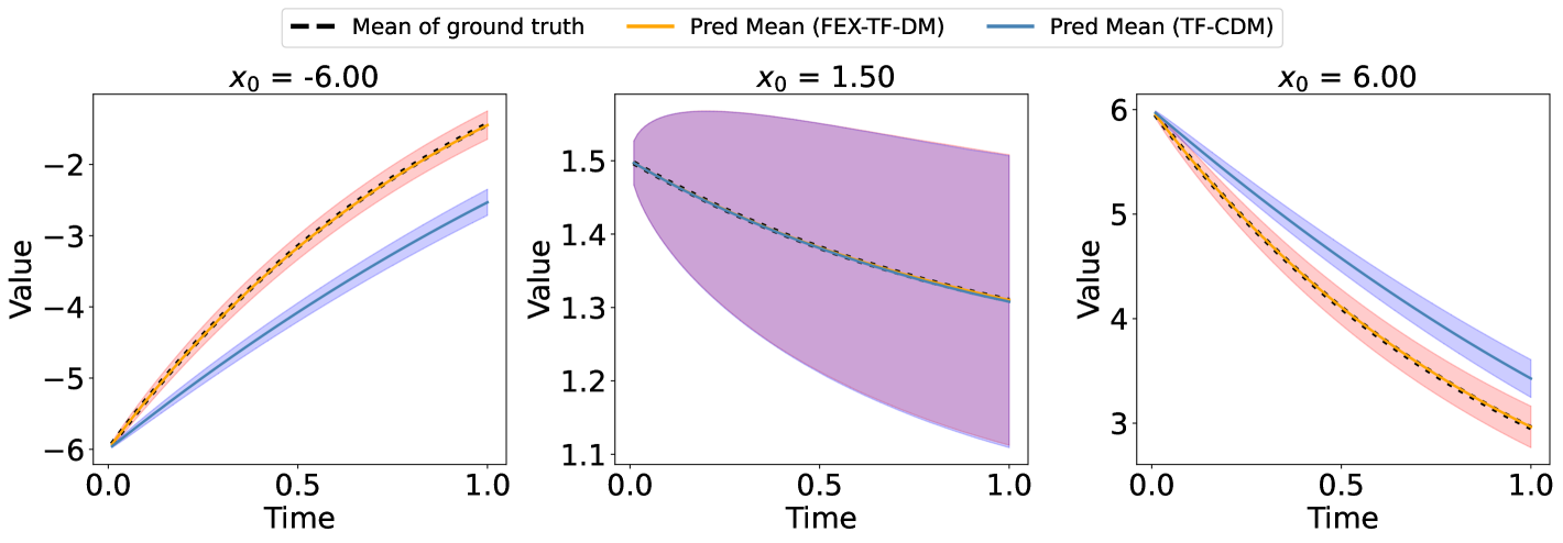
Fig. 3: Comparison of predicted mean trajectories and corresponding mean $\pm$ standard deviation bands of solutions for 1-dimensional OU process, evaluated at initial conditions $\mathbf{x}_{0}=-6,1.5,6$, obtained using the FEX-TF-DM, TF-CDM, and the ground truth.

Fig. 4: Comparison of conditional PDF $p_{\mathbf{x}_{t+\Delta t|\mathbf{x}_{t}}}(\mathbf{x}_{t+\Delta t}|\mathbf{x}_{t}=c)$ determined by FEX-TF-DM, TF-CDM and the ground truth for 1-dimensional OU process, with $c=-6,1.5,6$ at $t=0$, respectively.

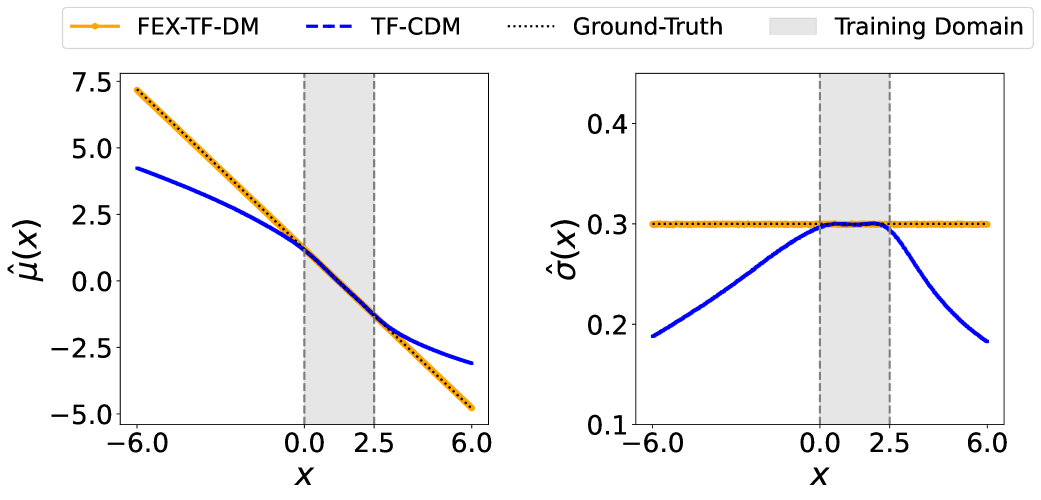
Fig. 5: Comparison of drift and diffusion functions obtained by the FEX-TF-DM, TF-CDM and the ground truth over domain $[-6,6]$ for 1-dimensional OU process. Left: drift term $\hat{\mu}(x)$; Right: diffusion term $\hat{\sigma}(x)$; The shaded region indicates the training domain $[0,2.5]$.

5.1.2 2-dimensional OU process

As a second example, we explore the two-dimensional OU process, which evolves according to the following SDE:

(29) $$d\mathbf{x}_{t}=B\mathbf{x}_{t}dt+\Sigma dW_{t},$$

where state variable $\mathbf{x}_{t}=({x}_{1},{x}_{2})\in\mathbb{R}^{2}$ evolves under the influence of the drift matrix $B$ and the diffusion matrix $\Sigma$, both defined as:

$$B=\begin{pmatrix}-1&-0.5\\ -1&-1\end{pmatrix},\quad\quad\Sigma=\begin{pmatrix}1&0\\ 0&0.5\\ \end{pmatrix}.$$

To build the dataset $\mathcal{D}_{\text{obs}}$, we simulate $35,000$ trajectories, generating a total of $350,000$ data points using (29). The initial states are uniformly sampled from $(-4,4)\times(-3,3)$ and integrated up to $T=1.0$. To recover the deterministic component $\mathbf{D}_{\theta_{1}}(\mathbf{x}_{t})$, we randomly choose 60,000 initial states from $\mathcal{D}_{\text{obs}}$ and apply FEX to derive an analytical expression. Following the one-dimensional setup, we construct two binary tree models and incorporate the dimension-adaptive formulation from (11). The resulting expressions are shown in Table 2, where the learned drift closely matches the ground truth. Although additional nonlinear terms appear in the approximation, the framework $\mathbf{G}_{\theta}$ is designed to reduce their effect and ensure accurate modeling of true system behavior.

True Drift Expression (2D)	Best Approximation for $\mathbf{D}_{\theta_{1}}(\mathbf{x}_{t})$ (2D)
$-{x}_{1}-0.5{x}_{2}$	$-0.9835{x}_{1}-0.4917{x}_{2}$
	$-0.0004515{x}_{1}^{5}+0.0015927{x}_{1}{x}_{2}^{4}-0.0002257{x}_{1}^{4}{x}_{2}$
	$+0.0007969{x}_{1}^{5}+0.0002689{x}_{1}^{4}-0.0009491{x}_{2}^{4}+0.2996$
$-{x}_{1}-{x}_{2}$	$-0.9869{x}_{1}-0.9642{x}_{2}$
	$-0.0133\sin({x}_{1})-0.0355\sin({x}_{2})+0.0165$

Table 2: Comparison of true drift term and the FEX-learned deterministic component.

To label the training data, we construct a dataset $\mathcal{D}_{\text{label}}$ using these 60,000 selected states. Once the model $\mathbf{G}_{\theta}$ is trained, we generate 65,000 predicted trajectories and extend the simulations to $T=5.0$. Figure (6) illustrates how the predicted means and standard deviations of the solutions for initial conditions $\mathbf{x}_{0}=(5,4),(0.3,0.4)$ and $(-5,-4)$ align with the ground truth. Although training was limited to $T=1.0$, the model generalizes well, maintaining close agreement with the exact solutions throughout the extended time horizon. Furthermore, Figure (7) shows the one-step conditional probability distribution $p_{\mathbf{x}_{t+\Delta t}|\mathbf{x}_{t}}(\mathbf{x}_{t+\Delta t}|\mathbf{x}_{t}=(0,0))$, demonstrating that the predicted distribution effectively replicates the true stochastic behavior of the system.

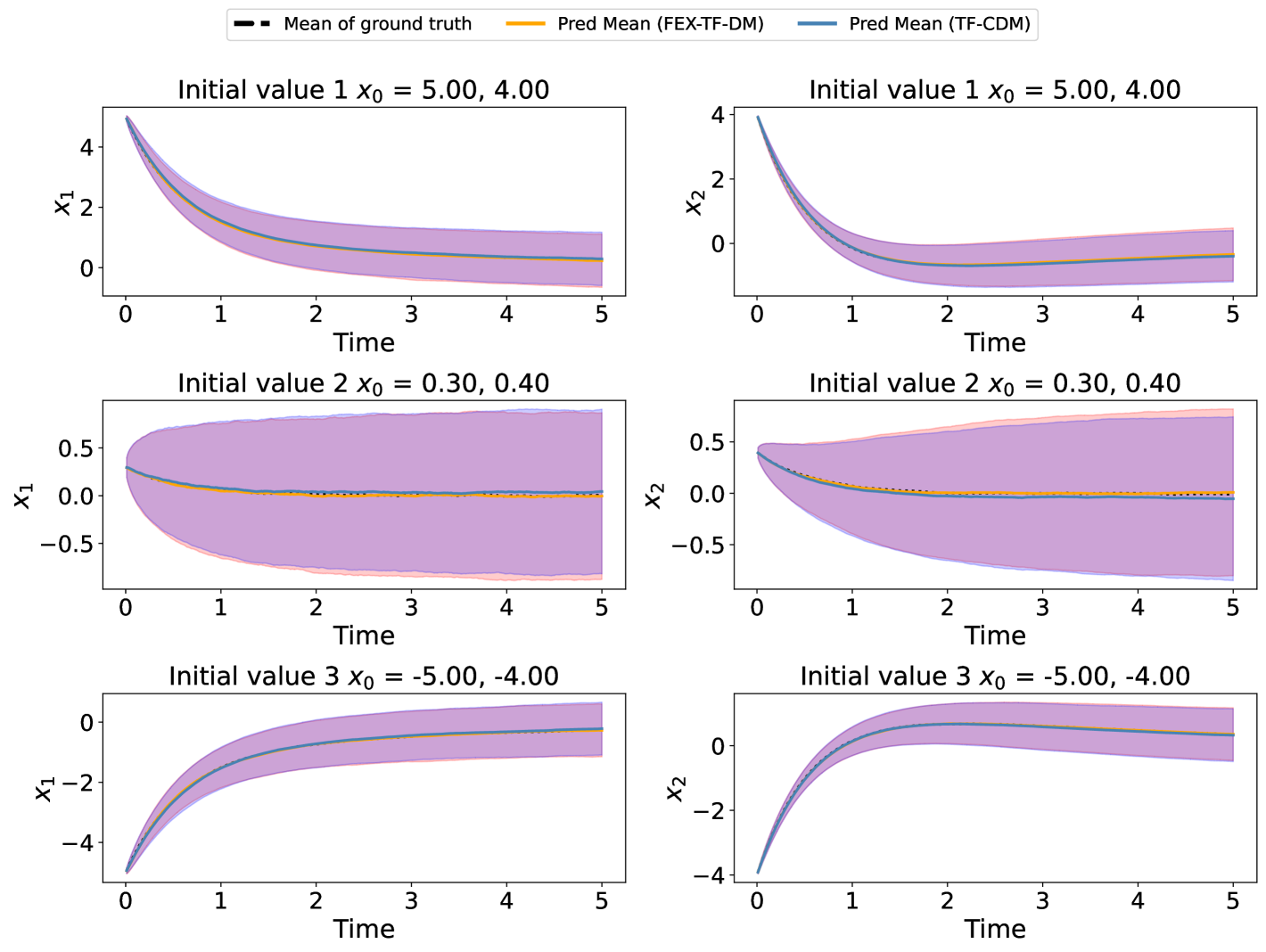
Fig. 6: Comparison of predicted mean trajectories and corresponding mean $\pm$ standard deviation bands of solutions for 2-dimensional OU process, evaluated at initial conditions $\mathbf{x}_{0}=(5,4),(0.3,0.4)(-5,-4)$, obtained using the FEX-TF-DM, TF-CDM, and the ground truth.

Fig. 7: Comparison of conditional PDF $p_{\mathbf{x}_{t+\Delta t|\mathbf{x}_{t}}}(\mathbf{x}_{t+\Delta t}|\mathbf{x}_{t}=(0.3,0.4))$ determined by FEX-TF-DM, TF-CDM and the ground truth for 2-dimensional OU process at $t=0$.

5.2 Nonlinear SDEs

We now consider It$\hat{o}$ type SDEs with nonlinear drift and diffusion functions. These models capture complex stochastic dynamics beyond linear approximations, making them essential for describing real-world phenomena influenced by randomness. In this section, we focus on three representative examples as follows.

5.2.1 1-dimensional SDE with trigonometric drift

The SDE with trigonometric drift is defined by

(30) $$d\mathbf{x}_{t}=\sin(2m\pi\mathbf{x}_{t})dt+\sigma dW_{t},$$

where $m=1$ and $\sigma=0.8$. The observation dataset $\mathcal{D}_{\text{obs}}$ comprises 100,000 data pairs from $L=10,000$ trajectories, obtained by solving the SDE in (30) with initial values uniformly sample from $\mathcal{U}(0,1)$ up to $T=1.0$. To estimate the deterministic component $\mathbf{D}_{\theta_{1}}(\mathbf{x}_{t})$, we randomly choose 60,000 initial states from $\mathcal{D}_{\text{obs}}$. Using the approach described in Section 3 to derive a closed-form expression, presented in Table 3.

True drift expression	Best expression for $\mathbf{D}_{\theta_{1}}(\mathbf{x}_{t})$
$\sin(2\pi\mathbf{x}_{t})$	$-1.1989\cos(6.2476\mathbf{x}_{t}-4.6837)-0.0104$

Table 3: Comparison of true drift term and the FEX-learned deterministic component.

We generate labeled training data points and use them to train the model $\mathbf{G}_{\theta}$, after which we simulate 500,000 prediction trajectories extending to $T=5.0$. The performance of the model is evaluated for the initial conditions $\mathbf{x}_{0}=-3,0.5,3$, and the results are compared against the ground truth in Figure 8. This figure offers a direct comparison between the predicted and actual solutions. Although the model was trained only up to $T=1.0$, it accurately captures both the mean and the standard deviation of the true dynamics over the extended time interval, highlighting its strong generalizability beyond the training horizon. Furthermore, Figure (9) shows the one-step conditional distributions at $t=0$ for each of the initial conditions chosen. The predicted distributions are in close agreement with the exact distributions, indicating that the model effectively captures the underlying stochastic behavior.

Furthermore, Figure 10 shows the effective drift and diffusion functions learned by the model, compared with the true functions in an extended domain over an extended domain $[-5,5]$, beyond the original training interval of $(0,1)$. The learned terms match the true functions well within the training region and continue to exhibit consistent behavior beyond it. This consistency suggests that the model not only learns accurate representations of the dynamics but also maintains robustness when extrapolating to unseen regions of the domain.

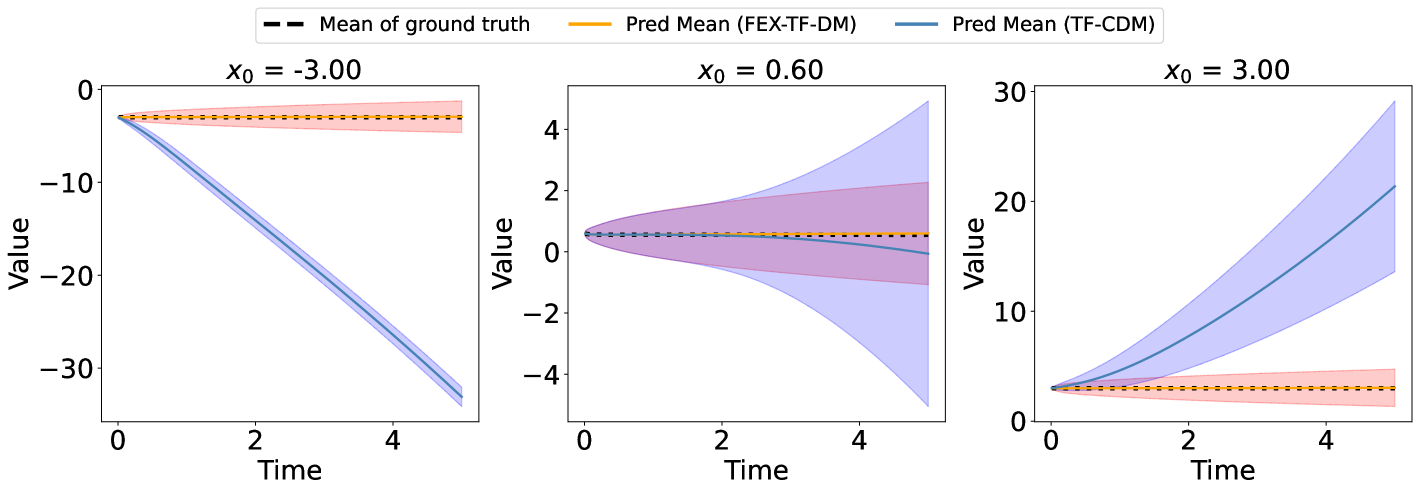
Fig. 8: Comparison of predicted mean trajectories and corresponding mean $\pm$ standard deviation bands of solutions for SDE with trigonometric drift, evaluated at initial conditions $\mathbf{x}_{0}=-3,0.6,3$, obtained using the FEX-TF-DM, TF-CDM, and the ground truth.

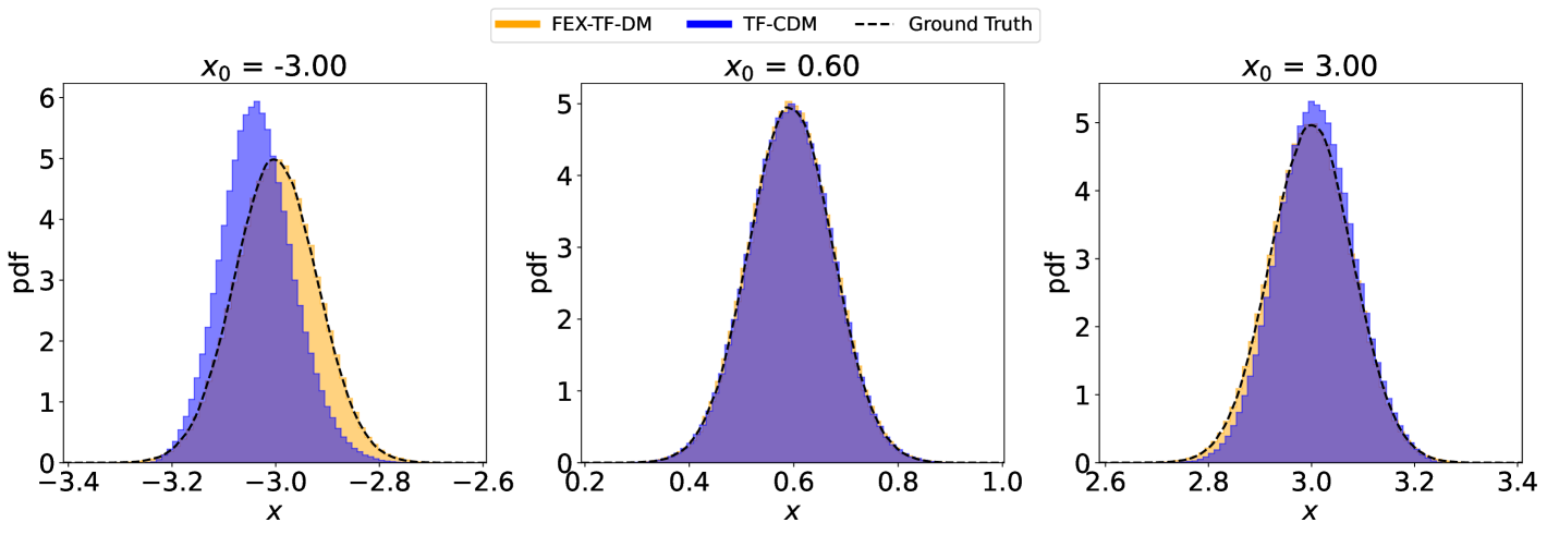
Fig. 9: Comparison of conditional PDF $p_{\mathbf{x}_{t+\Delta t|\mathbf{x}_{t}}}(\mathbf{x}_{t+\Delta t}|\mathbf{x}_{t}=c)$ determined by FEX-TF-DM, TF-CDM and the ground truth for SDE with trigonometric drift, with $c=-3,0.6,3$ at $t=0$, respectively.

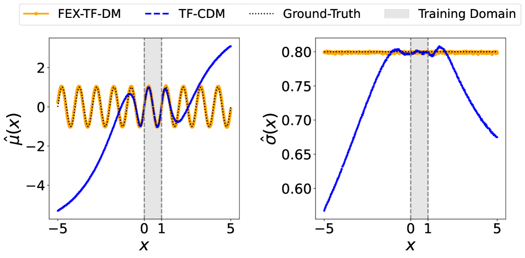
Fig. 10: Comparison of drift and diffusion functions obtained by the FEX-TF-DM, TF-CDM and the ground truth over domain $[-5,5]$ for SDE with trigonometric drift. Left: drift term $\hat{\mu}(x)$; Right: diffusion term $\hat{\sigma}(x)$; The shaded region indicates the training domain $[0,1]$.

5.2.2 1-dimensional SDE with Double-Well Potential

We consider an SDE with a double-well potential:

$$dx_{t}=(x_{t}-x_{t}^{3})dt+\sigma dW_{t},$$

where $\sigma=0.5$. There are two stable states at $x=-1$ and $x=1$, and the system can randomly transition between these two stable states over time. The observation dataset $\mathcal{D}_{\text{obs}}$ consists of 10,0000 data pairs from $L=10,000$ trajectories, obtained by solving the SDE in (30) with the initial values uniformly sampled from $\mathcal{U}(-2,2)$ up to $T=1.0$. To estimate the deterministic component $\mathbf{D}_{\theta_{1}}(\mathbf{x}_{t})$, we randomly choose 60,000 initial states from $\mathcal{D}_{\text{obs}}$. Using the approach described in Section 3 to derive a closed-form expression, presented in Table 4.

True drift expression	Best expression for $\mathbf{D}_{\theta_{1}}(\mathbf{x}_{t})$
$\mathbf{x}_{t}-\mathbf{x}_{t}^{3}$	$-0.9922\mathbf{x}_{t}^{3}+0.9709\mathbf{x}_{t}+0.0019$

Table 4: Comparison of true drift term and the FEX-learned deterministic component.

We simulate 500,000 prediction trajectories up to $T=5.0$ to test the trained model $\mathbf{G}_{\theta}$. The predicted solutions for the initial values $\mathbf{x}_{0}=-5,1.5,5$ are compared with the ground truth in Figure 11, which provides a side-by-side visualization of the predicted and exact results. Although the model is only trained with data up to $T=1.0$, it successfully captures the mean and standard deviation of the true solution over the extended time interval, demonstrating strong generalization performance up to $T=5.0$. In addition, Figure 12 shows the trajectories from $\mathbf{x}_{0}=1.5$ to $T=500$, clearly revealing the presence of the well potential within the dynamics.

Furthermore, Figure 13 illustrates the one-step conditional distributions at $t=0$ for the initial values $\mathbf{x}_{0}=-5,1.5,5$, respectively. The predicted distributions closely match the exact ones, further validating the model’s ability to accurately capture and maintain key stochastic properties. And we also show the evolution of the solution for case $\mathbf{x}_{0}=1.5$ at times $t=5,\ 10,\ 30,\ 100$ in Figure 14. Finally, Figure 15 compares the learned drift and diffusion functions with the true functions in an extended domain $[-5,5]$, beyond the original interval $(-2,2)$. The results show that the learned terms remain accurate within the training region and extend reliably to unseen areas. This indicates that the model not only fits the known data well, but also exhibits strong extrapolation ability, maintaining asymptotic consistency and further reinforcing its robustness.

Fig. 11: Comparison of predicted mean trajectories and corresponding mean $\pm$ standard deviation bands of solutions for SDE with double well potential, evaluated at initial conditions $\mathbf{x}_{0}=-5,1.5,5$, obtained using the FEX-TF-DM, TF-CDM, and the ground truth.

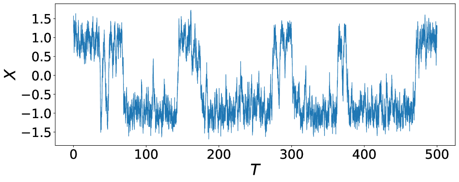
Fig. 12: Solution trajectory for time up to $T=500$ when $\mathbf{x}_{0}=1.5$.

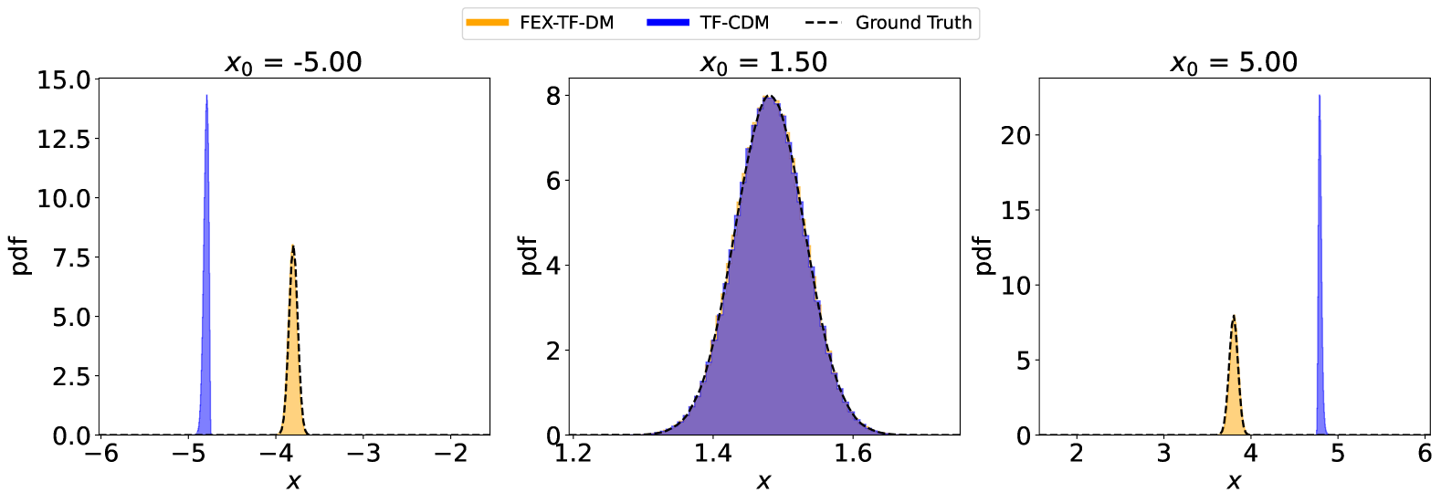
Fig. 13: Comparison of conditional PDF $p_{\mathbf{x}_{t+\Delta t|\mathbf{x}_{t}}}(\mathbf{x}_{t+\Delta t}|\mathbf{x}_{t}=c)$ determined by FEX-TF-DM, TF-CDM and the ground truth for SDE with double well potential, with $c=-5,1.5,5$ at $t=0$, respectively.

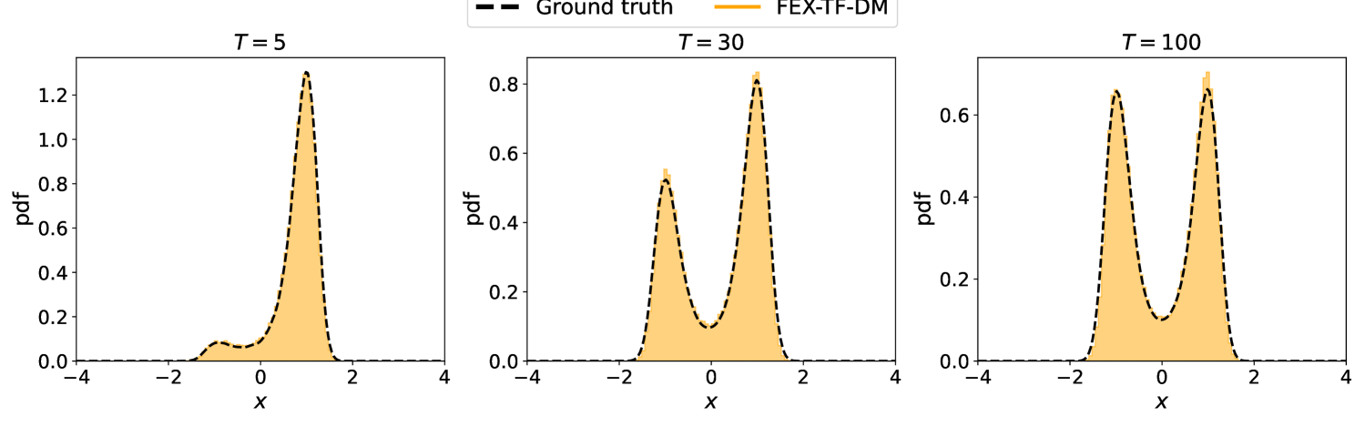
Fig. 14: Evolution of conditional PDF $p_{\mathbf{x}_{t+\Delta t|\mathbf{x}_{t}}}(\mathbf{x}_{t+\Delta t}|\mathbf{x}_{t}=1.5)$ determined by FEX-TF-DM and the ground truth for SDE with double well potential, at $t=5,30,100$, respectively.

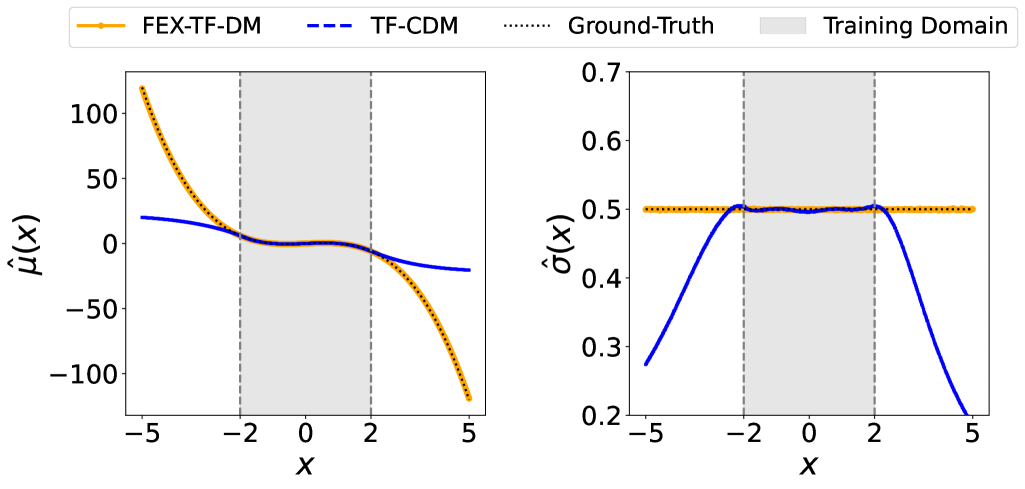
Fig. 15: Comparison of the drift and diffusion functions learned by FEX-TF-DM and TF-CDM against the ground truth over the domain $[-5,5]$ for the SDE with double well potential. Left: drift term $\hat{\mu}(x)$; Right: diffusion term $\hat{\sigma}(x)$; The shaded region indicates the training domain $[-2,2]$.

5.2.3 2-dimensional OL process

We consider a two-dimensional OL process governed by the following SDE:

(31) $$d\mathbf{x}_{t}=-\nabla V(\mathbf{x}_{t})dt+\Sigma dW_{t},$$

where the state variable is $\mathbf{x}_{t}=({x}_{1},{x}_{2})\in\mathbb{R}^{2}.$ And the drift term is derived from the potential function:

$$V(\mathbf{x}_{t})=2.5({x}_{1}^{2}-1)^{2}+5{x}_{2}^{2},$$

with diffusion function by:

$$\Sigma=\begin{pmatrix}\sqrt{2}&0\\ 0&\sqrt{2}\end{pmatrix}.$$

The corresponding simulation of the potential function $V(\mathbf{x}_{t})$ and its contour is illustrated in the following figure.

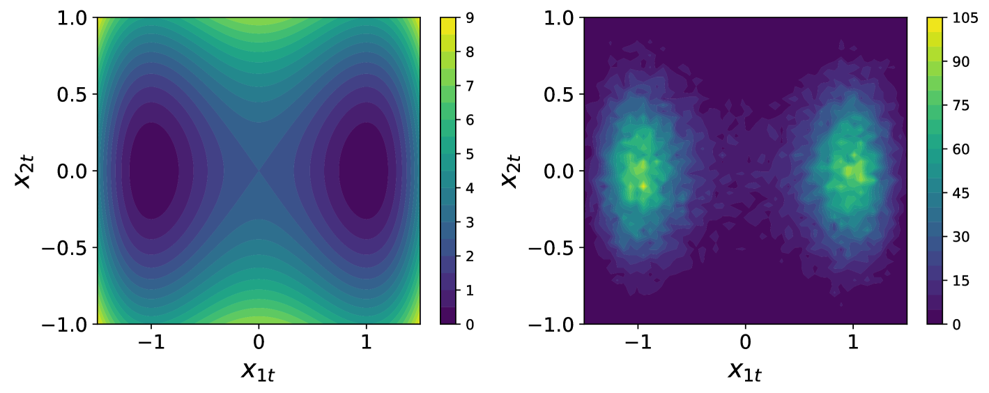
Fig. 16: Visualization of the potential function $V(\mathbf{x}_{t})$ and the corresponding density of particle positions. The left plot illustrates the contour of the potential function. And The right plot displays the density distribution of particle positions over time.

The observation dataset $\mathcal{D}_{\text{obs}}$ comprises $350,000$ data pairs collected from $L=35,000$ trajectories, generated by SDE in (29) with initial values uniformly sampled from $(-1.5,1.5)\times(-1,1)$ to $T=1.0$. To estimate the deterministic component $\hat{D}_{\theta_{1}}(\mathbf{x}_{t})$, we randomly select 60,000 initial states from $\mathcal{D}_{\text{obs}}$ and apply the FEX to derive an analytical expression. Following the one-dimensional setup, we construct two binary tree models and incorporate the dimension-adaptive formulation from (11). The resulting expressions are shown in Table 5, where the learned drift closely matches the ground truth. Although additional nonlinear terms appear in the approximation, the framework $\mathbf{G}_{\theta}$ is designed to reduce their effect and ensure accurate modeling of true system behavior.

True Drift Expression (2D)	Best Approximation for $\hat{D}_{\theta_{1}}(\mathbf{x}_{t})$ (2D)
$-10{x}_{1}({x}_{1}^{2}-1)$	$-9.9178{x}_{1}^{3}+0.1625{x}_{2}^{3}$
	$+9.8165{x}_{1}+0.1204{x}_{2}+0.03$
$-10{x}_{2}$	$-0.0613{x}_{1}-9.9911{x}_{2}+0.0011$

Table 5: Comparison of true drift term and the FEX-learned deterministic component.

We also construct the labeled training data $\mathcal{D}_{\text{label}}$ from the observation dataset. After training the model $\mathbf{G}_{\theta}$, we simulate 65,000 predictive trajectories up to $T=5.0$. Figure (17) shows the predicted results for initial values $\mathbf{x}_{0}=(-3,-3),(0.6,0.6)$ and $(3,3)$, compared to the ground truth. Although trained only on data up to $T=1.0$, the model demonstrates a strong generalizability, accurately reproducing the mean and standard deviation of the true solution over the extended time range. Furthermore, Figure (18) illustrates the one-step conditional probability distribution $p_{\mathbf{x}_{t+\Delta t}|\mathbf{x}_{t}}(\mathbf{x}_{t+\Delta t}|\mathbf{x}_{t}=(0.6,0.6))$, demonstrating that the predicted distribution effectively replicates the true stochastic behavior of the system.

Lastly, Figure 19 compares the effective drift and diffusion functions with the ground truth in an extended domain $[-5,5]\times[-5,5]$, rather than the original domain. The observation is that the learned functions remain accurate within the training interval and continue to behave consistently in extrapolated regions.

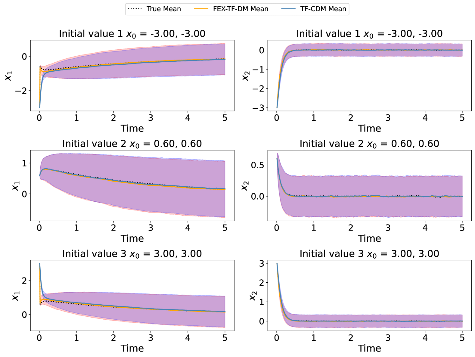
Fig. 17: Comparison of the mean and the standard deviation of solutions for $\mathbf{x}_{0}=(-3,-3),(0.6,0.6)$, and $(3,3)$, obtained by the FEX-TF-DM, TF-CDM and the ground truth for SDE with OL process.

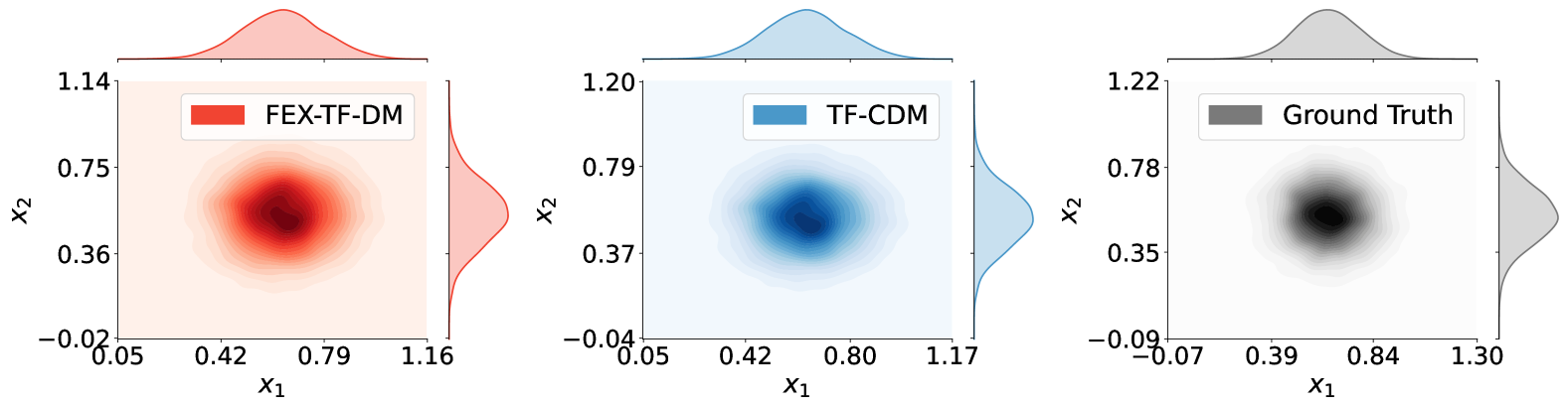
Fig. 18: Comparison of conditional PDF $p_{\mathbf{x}_{t+\Delta t|\mathbf{x}_{t}}}(\mathbf{x}_{t+\Delta t}|\mathbf{x}_{t}=(0.6,0.6))$ determined by FEX-TF-DM, TF-CDM and the ground truth for OL process at $t=0$.

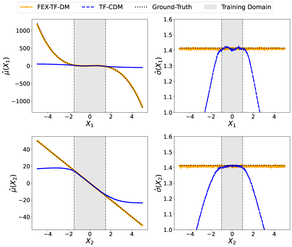
Fig. 19: Comparison of drift and diffusion functions obtained by the FEX-TF-DM and the ground truth over domain $[-5,5]$ for the SDE with OL process. Here $\hat{u}(\mathbf{x}_{1})$ and $\hat{u}(\mathbf{x}_{2})$ are the expressions in the second column of Table 5. $\hat{\sigma}(\mathbf{x}_{1})$ and $\hat{\sigma}(\mathbf{x}_{2})$ are $\sqrt{2}$ in this case.

5.3 SDEs with Non-Gaussian Noise

In this section, we consider a 1-dimensional SDE driven by exponential distribution as following:

(32) $$d\mathbf{x}_{t}=\mu\mathbf{x}_{t}dt+\sigma\sqrt{dt}\eta_{t},\quad\eta_{t}\sim\text{exp}(1),$$

where $\eta_{t}$ has an exponential PDF $f_{\eta}(x)=e^{-x},x\geq 0$, and $\mu=-2.0,\sigma=0.1$. The observation dataset $\mathcal{D}_{\text{obs}}$ is constructed by generating $L=10,000$ trajectories samples, obtained by solving (32) with initial values uniformly sampled from $\mathcal{U}(0,2.5)$ to $T=1.0$. To estimate the deterministic component $\mathbf{D}_{\theta_{1}}(\mathbf{x}_{t})$, we randomly choose 60,000 initial states from $\mathcal{D}_{\text{obs}}$ and apply the principles discussed in Section 3 to derive an analytic representation, as presented in Table 6.

True drift expression	Best expression for $\mathbf{D}_{\theta_{1}}(\mathbf{x}_{t})$
$-2\mathbf{x}_{t}$	$-1.9750528\mathbf{x}_{t}$

Table 6: Comparison of true drift term and the FEX-learned deterministic component.

The predicted solutions generated by the model are compared with the ground truth in Figure 20 for the initial value for the initial values $\mathbf{x}_{0}=-1,1.5,4$, respectively. In particular, the values $\mathbf{x}_{0}=-1$ and $\mathbf{x}_{0}=4$ are outside the training domain of $(0,2.5)$. However, the model accurately tracks the true solution up to $T=5.0$, highlighting its strong generalization capability beyond the training horizon of $T=1.0$. Figure 21shows the one-step conditional distributions predicted for each initial value, which closely match the corresponding true distributions. This consistency further confirms the model’s ability to capture and preserve the underlying stochastic behavior.

Furthermore, Figure 22 presents the effective drift and diffusion function curves alongside the true drift $\mu$ and the diffusion function $\sigma$ in an extended domain $[-2,10]$, compared to the training range $(0,2.5)$. The results indicate that the model not only captures the true dynamics accurately within the training region but also generalizes effectively to a broader domain. This suggests that the learned functions remain asymptotically consistent as the input domain expands toward larger values.

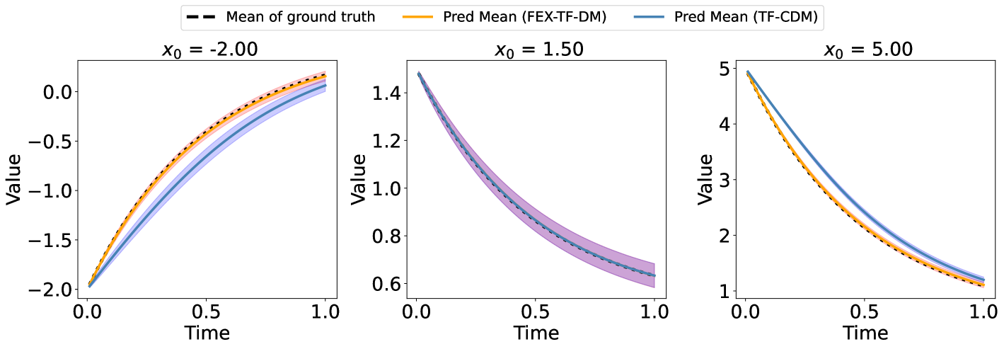
Fig. 20: Comparison of predicted mean trajectories and corresponding mean $\pm$ standard deviation bands for solutions to the SDE with exponential diffusion, evaluated at initial conditions $\mathbf{x}_{0}=-2,1.5,5$, obtained using the FEX-TF-DM, TF-CDM, and the ground truth.

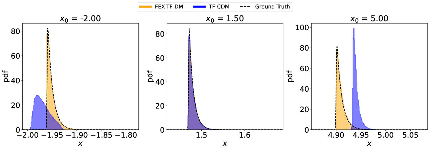
Fig. 21: Comparison of conditional PDF $p_{\mathbf{x}_{t+\Delta t|\mathbf{x}_{t}}}(\mathbf{x}_{t+\Delta t}|\mathbf{x}_{t}=c)$ estimated by FEX-TF-DM, TF-CDM, and the ground truth for the SDE with exponential diffusion, with $c=-2,1.5,5$ at $t=0$, respectively.

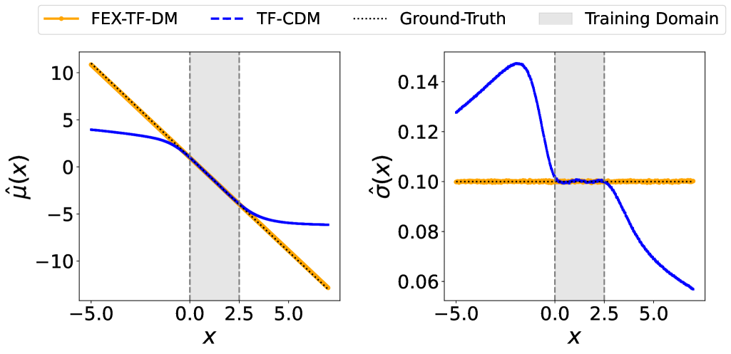
Fig. 22: Comparison of the drift and diffusion functions learned by FEX-TF-CDM, TF-CDM and the ground truth over the domain $[-5,7]$ for the SDE with exponential diffusion. Left: drift term $\hat{\mu}(x)$; Right: diffusion term $\hat{\sigma}(x)$; The shaded region indicates the training domain $[0,2.5]$.

6 Discussion and perspectives

This paper introduces a novel framework for modeling SDEs that combines explicit mathematical representations of the deterministic component - derived via a finite expression method - with complementary techniques for modeling the stochastic component. The approach prioritizes transparency and interpretability, avoiding dependence on black-box neural architectures. By learning closed-form expressions directly from the data, the model demonstrates strong predictive performance across a wide range of stochastic systems. It generalizes well beyond the training domain, accurately captures both short- and long-term dynamics, and effectively models complex behaviors in linear, nonlinear, and multidimensional settings. In particular, the learned drift and diffusion terms remain consistent in the extrapolated regions, which highlights the flexibility of the method.

Despite these promising results, several extensions could further improve and broaden the approach. First, incorporating state-dependent or control-dependent diffusion functions would allow the model to represent more complex systems, including those exhibiting nonlocal behavior or critical transitions. Second, extending the framework to accommodate non-autonomous systems, where system properties evolve explicitly over time, would expand its applicability to time-varying environments. Third, adapting the model to handle more advanced stochastic structures, such as jump processes or systems driven by fractional Brownian motion, could increase its utility in domains like finance, neuroscience, and climate science. Finally, a deeper theoretical investigation of the underlying mechanisms of the score-based sampling strategy, particularly its convergence properties and error bounds, would provide stronger guarantees and insight into the foundations of the method. These directions highlight the potential for continued development of mathematically grounded and interpretable approaches for learning and simulating complex stochastic systems.

7 Acknowledgements

The research of Chunmei Wang was partially supported by National Science Foundation Grant DMS-2206332. This material was based upon work supported by the U.S. Department of Energy, Office of Science, Office of Advanced Scientific Computing Research SciDAC program under Contract No. DE-AC02-05CH11231.

References

- [1] Thomas Bose and Steffen Trimper. Stochastic model for tumor growth with immunization. Physical Review E—Statistical, Nonlinear, and Soft Matter Physics, 79(5):051903, 2009.
- [2] Lulu Cao, Zimo Zheng, Chenwen Ding, Jinkai Cai, and Min Jiang. Genetic programming symbolic regression with simplification-pruning operator for solving differential equations. In International Conference on Neural Information Processing, pages 287–298. Springer, 2023.
- [3] Xiaoli Chen, Jinqiao Duan, Jianyu Hu, and Dongfang Li. Data-driven method to learn the most probable transition pathway and stochastic differential equation. Physica D: Nonlinear Phenomena, 443:133559, 2023.
- [4] Yuan Chen and Dongbin Xiu. Learning stochastic dynamical system via flow map operator. Journal of Computational Physics, 508:112984, 2024.
- [5] Yuan Chen and Dongbin Xiu. Modeling unknown stochastic dynamical system subject to external excitation. arXiv preprint arXiv:2406.15747, 2024.
- [6] Kai Leong Chong, Jun-Qiang Shi, Guang-Yu Ding, Shan-Shan Ding, Hao-Yuan Lu, Jin-Qiang Zhong, and Ke-Qing Xia. Vortices as brownian particles in turbulent flows. Science advances, 6(34):eaaz1110, 2020.
- [7] William Coffey and Yu P Kalmykov. The Langevin equation: with applications to stochastic problems in physics, chemistry and electrical engineering, volume 27. World Scientific, 2012.
- [8] Rama Cont and Peter Tankov. Financial modelling with jump processes. Chapman and Hall/CRC, 2003.
- [9] Miles Cranmer, Alvaro Sanchez Gonzalez, Peter Battaglia, Rui Xu, Kyle Cranmer, David Spergel, and Shirley Ho. Discovering symbolic models from deep learning with inductive biases. Advances in neural information processing systems, 33:17429–17442, 2020.
- [10] Jianda Du, Senwei Liang, and Chunmei Wang. Learning epidemiological dynamics via the finite expression method. arXiv preprint arXiv:2412.21049, 2024.
- [11] Albert Einstein. Über die von der molekularkinetischen theorie der wärme geforderte bewegung von in ruhenden flüssigkeiten suspendierten teilchen. Annalen der physik, 4, 1905.
- [12] JN Elgin. The fokker-planck equation: methods of solution and applications. Optica Acta: International Journal of Optics, 31(11):1206–1207, 1984.
- [13] Stephanie Forrest. Genetic algorithms: principles of natural selection applied to computation. Science, 261(5123):872–878, 1993.
- [14] C Gardiner. Stochastic methods: A handbook for the natural and social sciences fourth edition (2009).
- [15] CW Gardiner. Handbook of stochastic methods, eds. 4th, 2009.
- [16] Yiqi Gu, John Harlim, Senwei Liang, and Haizhao Yang. Stationary density estimation of itô diffusions using deep learning. SIAM Journal on Numerical Analysis, 61(1):45–82, 2023.
- [17] Peter Hänggi, Peter Talkner, and Michal Borkovec. Reaction-rate theory: fifty years after kramers. Reviews of modern physics, 62(2):251, 1990.
- [18] Tong He, Zhi Zhang, Hang Zhang, Zhongyue Zhang, Junyuan Xie, and Mu Li. Bag of tricks for image classification with convolutional neural networks. In Proceedings of the IEEE/CVF conference on computer vision and pattern recognition, pages 558–567, 2019.
- [19] Nan Jiang and Yexiang Xue. Symbolic regression via control variable genetic programming. In Joint European Conference on Machine Learning and Knowledge Discovery in Databases, pages 178–195. Springer, 2023.
- [20] Zhongyi Jiang, Chunmei Wang, and Haizhao Yang. Finite expression methods for discovering physical laws from data. arXiv preprint arXiv:2305.08342, 2023.
- [21] Richard Jordan, David Kinderlehrer, and Felix Otto. The variational formulation of the fokker–planck equation. SIAM journal on mathematical analysis, 29(1):1–17, 1998.
- [22] Pierre-Alexandre Kamienny, Stéphane d’Ascoli, Guillaume Lample, and François Charton. End-to-end symbolic regression with transformers. Advances in Neural Information Processing Systems, 35:10269–10281, 2022.
- [23] Ioannis Karatzas and Steven Shreve. Brownian motion and stochastic calculus, volume 113. Springer Science & Business Media, 1991.
- [24] Takeaki Kariya, Regina Y Liu, Takeaki Kariya, and Regina Y Liu. Options, futures and other derivatives. Asset Pricing: -Discrete Time Approach-, pages 9–26, 2003.
- [25] GABRIEL GEORGE Katul, Amilcare Porporato, R Nathan, M Siqueira, MB Soons, Davide Poggi, HS Horn, and SA Levin. Mechanistic analytical models for long-distance seed dispersal by wind. The American Naturalist, 166(3):368–381, 2005.
- [26] Hendrik Anthony Kramers. Brownian motion in a field of force and the diffusion model of chemical reactions. physica, 7(4):284–304, 1940.
- [27] Wenqiang Li, Weijun Li, Linjun Sun, Min Wu, Lina Yu, Jingyi Liu, Yanjie Li, and Songsong Tian. Transformer-based model for symbolic regression via joint supervised learning. In The Eleventh International Conference on Learning Representations, 2022.
- [28] Senwei Liang and Haizhao Yang. Finite expression method for solving high-dimensional partial differential equations. arXiv preprint arXiv:2206.10121, 2022.
- [29] Benjamin Lindner and Lutz Schimansky-Geier. Transmission of noise coded versus additive signals through a neuronal ensemble. Physical review letters, 86(14):2934, 2001.
- [30] Yanfang Liu, Yuan Chen, Dongbin Xiu, and Guannan Zhang. A training-free conditional diffusion model for learning stochastic dynamical systems. arXiv preprint arXiv:2410.03108, 2024.
- [31] Ziming Liu, Yixuan Wang, Sachin Vaidya, Fabian Ruehle, James Halverson, Marin Soljačić, Thomas Y Hou, and Max Tegmark. Kan: Kolmogorov-arnold networks. arXiv preprint arXiv:2404.19756, 2024.
- [32] Hongsup Oh, Roman Amici, Geoffrey Bomarito, Shandian Zhe, Robert Kirby, and Jacob Hochhalter. Genetic programming based symbolic regression for analytical solutions to differential equations. arXiv preprint arXiv:2302.03175, 2023.
- [33] Bernt Oksendal. Stochastic differential equations: an introduction with applications. Springer Science & Business Media, 2013.
- [34] Manfred Opper. Variational inference for stochastic differential equations. Annalen der Physik, 531(3):1800233, 2019.
- [35] Brenden K Petersen, Mikel Landajuela, T Nathan Mundhenk, Claudio P Santiago, Soo K Kim, and Joanne T Kim. Deep symbolic regression: Recovering mathematical expressions from data via risk-seeking policy gradients. arXiv preprint arXiv:1912.04871, 2019.
- [36] Tong Qin, Kailiang Wu, and Dongbin Xiu. Data driven governing equations approximation using deep neural networks. Journal of Computational Physics, 395:620–635, 2019.
- [37] Georgios Rigas, Aimee S Morgans, RD Brackston, and Jonathan F Morrison. Diffusive dynamics and stochastic models of turbulent axisymmetric wakes. Journal of Fluid Mechanics, 778:R2, 2015.
- [38] Tim Salimans, Ian Goodfellow, Wojciech Zaremba, Vicki Cheung, Alec Radford, and Xi Chen. Improved techniques for training gans. Advances in neural information processing systems, 29, 2016.
- [39] Michael Schmidt and Hod Lipson. Distilling free-form natural laws from experimental data. science, 324(5923):81–85, 2009.
- [40] Zezheng Song, Chunmei Wang, and Haizhao Yang. Finite expression method for learning dynamics on complex networks. arXiv preprint arXiv:2401.03092, 2024.
- [41] Richard S Sutton. Reinforcement learning: An introduction. A Bradford Book, 2018.
- [42] Silviu-Marian Udrescu and Max Tegmark. Ai feynman: A physics-inspired method for symbolic regression. Science advances, 6(16):eaay2631, 2020.
- [43] George E Uhlenbeck and Leonard S Ornstein. On the theory of the brownian motion. Physical review, 36(5):823, 1930.
- [44] Oldrich Vasicek. An equilibrium characterization of the term structure. Journal of financial economics, 5(2):177–188, 1977.
- [45] Shu Wei, Yanjie Li, Lina Yu, Min Wu, Weijun Li, Meilan Hao, Wenqiang Li, Jingyi Liu, and Yusong Deng. Closed-form symbolic solutions: A new perspective on solving partial differential equations. arXiv preprint arXiv:2405.14620, 2024.
- [46] Darren J Wilkinson. Stochastic modelling for quantitative description of heterogeneous biological systems. Nature Reviews Genetics, 10(2):122–133, 2009.
- [47] Zhongshu Xu, Yuan Chen, Qifan Chen, and Dongbin Xiu. Modeling unknown stochastic dynamical system via autoencoder. Journal of Machine Learning for Modeling and Computing, 5(3), 2024.
- [48] Minglei Yang, Pengjun Wang, Diego del Castillo-Negrete, Yanzhao Cao, and Guannan Zhang. A pseudoreversible normalizing flow for stochastic dynamical systems with various initial distributions. SIAM Journal on Scientific Computing, 46(4):C508–C533, 2024.