Machine Learning Approach towards Quantum Error Mitigation for Accurate Molecular Energetics
Abstract
Despite significant efforts, the realization of the hybrid quantum-classical algorithms has predominantly been confined to proof-of-principles, mainly due to the hardware noise. With fault-tolerant implementation being a long-term goal, going beyond small molecules with existing error mitigation (EM) techniques with current noisy intermediate scale quantum (NISQ) devices has been a challenge. That being said, statistical learning methods are promising approaches to learning the noise and its subsequent mitigation. We devise a graph neural network and regression-based machine learning (ML) architecture for practical realization of EM techniques for molecular Hamiltonian without the requirement of the exponential overhead. Given the short coherence time of the quantum hardware, the ML model is trained with either ideal or mitigated expectation values over a judiciously chosen ensemble of shallow sub-circuits adhering to the native hardware architecture. The hardware connectivity network is mapped to a directed graph which encodes the information of the native gate noise profile to generate the features for the neural network. The training data is generated on-the-fly during ansatz construction thus removing the computational overhead. We demonstrate orders of magnitude improvements in predicted energy over a few strongly correlated molecules.
I introduction
Finding the exact ground state of general many-body systems is computationally hard and belongs to classically intractable problems[1, 2]. In fact, finding the ground state of a -local Hamiltonian is QMA-complete [3]. Nevertheless, with recent advancements in developing Noisy Intermediate-Scale Quantum (NISQ) devices[4, 5], handling the exponential scaling of resources has become tractable. Even though state-of-the-art quantum computers do not offer substantial quantum advantages due to quantum decoherence and a limited number of qubits, there has been active research in developing quantum algorithms and error mitigation techniques to harness the potential of quantum computing which might even allow us to study emerging phenomena in physics and chemistry.
Variational Quantum Eigensolver (VQE)[6] is a promising near-term application to find the ground state energy as it is designed to run on noisy machines with low coherence time [7]. VQE takes the parameterized quantum ansatz , and classically optimizes parameters to reach the ground state of a given molecular Hamiltonian.
| (1) |
There has been an extensive study on the choice of ansatz [8, 9]. Within the domain of chemistry the unitary coupled cluster with singles and doubles (UCCSD)[8, 9, 10] ansatz has emerged as a prevalent choice for the trial wavefunction where the unitary is expressed as:
| (2) |
Here, is the excitation operator where are the occupied orbital indices and are the virtual orbital indices with respect to reference Hartree-Fock (HF) state. In our implementations, we’ve reduced excitation operators by focusing solely on the dominant ones in the unitary, as detailed in section II.1. Although VQE has been proven to be resilient to noise for smaller quantum systems, inherent noise present in the current quantum processors deteriorates the performance of VQE for larger many-body Hamiltonian and complex quantum circuits. The sampling complexity of the expectation value estimation within VQE scales as for given precision , leading to exponential runtime and thus preventing it from going beyond proof of principles[11]. The theory of quantum fault tolerance could be used to deal with noise in the long run; however, in the current NISQ era, focusing on mitigating the noise instead of eliminating it is practically more realistic. The most captivating feature of Quantum Error Mitigation (QEM) techniques is their ability to minimize the noise-induced distortion in expectation values calculated on noisy hardware. Current methods such as Zero Noise Extrapolation (ZNE)[12], Dynamical Decoupling [13, 14], Probabilistic Error Cancellation [15], etc rely on modifying the existing circuit into a logically equivalent circuit but with an increased number of gates and hence gate errors. The requirement of such additional mitigating circuits and exponential overheads make these methods impractical. Along with VQE, works have been done in the Projective Quantum Eigensolver (PQE)[16] framework using ZNE [17].
Statistical learning methods are known to learn complex functions underlying the input data very well and the field of QEM is no exception to such models, as they eliminate the need for extra mitigating circuit execution, reducing runtime overheads. Although initial machine learning (ML) exploration for QEM has shown promising results, [18, 19, 20, 21, 22, 23] they are limited to shallow circuits and small fermionic systems. Scalable and cost-efficient QEM techniques must be tested for molecular Hamiltonians for strongly correlated systems beyond two-electron as they pose the most versatile and diverse circuit classes. However, existing schemes face information-theoretic limitations, such as entanglement spreading. To achieve quantum advantage, entanglement is necessary, but it comes at the cost of rapid noise spreading. Even when operating at depth, estimating the expectation values of noiseless observables, in the worst-case scenario, requires a super-polynomial number of samples[24]. Many QEM strategies like ZNE use exponentially many samples with respect to circuit depth, implying that the information should quickly get degraded due to sequential noise effects, requiring exponential overhead to remove the accumulated error [25]. Hence such QEM strategy is primarily limited to model Hamiltonian and very shallow quantum circuits.
In this work, we develop GraphNetMitigator (GNM) - a combined Graph Neural Network (GNN) and regression-based learning model to mitigate the noisy expectation values obtained through VQE for strongly correlated molecular systems over their entire potential energy profile across diverse quantum devices. We use snippets of the entire circuit consisting of single- and two-body fermionic excitations for model training and use them to predict the mitigated expectation values for the complete ansatz. The use of GNN is motivated from the fact that graph representations are the best modeling choice for such type of data where the instances have a similar circuit structures but differ in terms of two-qubit gate connectivity. We dynamically generate a portion of noisy training data during ansatz construction to ensure runtime efficiency. To validate the robustness of the GNM, we train it in two different settings: (1) assuming access to the ideal quantum computer (simulator-generated expectation values are used as labels) and (2) assuming we do not have access to the fault-tolerant quantum computer. In the latter case, we generate the labels by sequentially mitigating quantum error (see supplementary materials for details) which was found to produce accurate energetics for shallow quantum circuits without additional mitigation circuits. We employed CNOT-efficient implementation throughout to reduce circuit depth drastically [26, 27]. The performance of the GNM is tested on linear and molecules across their dissociation energy surface with diverse noise profiles derived from real hardware. We also study the robustness of GNM over other QEM techniques with varied synthetic noise strengths.
II Theory
The current limitations of the hardware has motivated research to construct shallow dynamic ansatz that can be realized in NISQ hardware[28, 29]. In often cases, the construction of the dynamic ansatz relies on the evaluation of gradients[28] in quantum hardware and under noisy scenario, such ansatz are often sub-optimally expressive. We previously advocated the importance of minimizing (or entirely bypassing) the usage of quantum resources while the dynamic ansatze are constructed such that the resulting ansatze maintain the requisite expressibility[30, 31, 32]. Of course, their execution (through whatever method they are generated) in a quantum device requires additional EM routines for accurate prediction of energetics. In this manuscript, while our principal focus is to develop the ML based EM strategy for any arbitrary disentangled ansatz[10], we also propose a robust methodology that forms a dynamic ansatz in a noisy quantum architecture which is nearly identical to an ansatz constructed under noiseless environment from the same operator pool. Such an undertaking serves twin desirable goals: firstly, it automatically generates the features needed for the regressor of our subsequent ML model and more importantly, due to its compatibility with a sequential reference error mitigation (SREM) strategy that generates mitigated results (which are used as training labels) for sub-circuits on the fly as the ansatz gets constructed. In short, this entire workflow can be executed in noisy quantum device without any implicit or explicit dependence to the fault-tolerant qubits. In the following section, we begin with the dynamic ansatz construction strategy in a noisy environment and demonstrate how this strategy generates additional features that are used up by the ML regressor.
II.1 Construction of a Dynamic Ansatz in Noisy Architecture
For all the two-body excitations characterized by the hole-particle composite index tuple , we calculate the one-parameter energy functional by optimizing the single parameter circuits
| (3) |
where is the sole variational parameter in each such optimization. Furthermore, we calculate the "noisy" reference energy for each of these one-parameter circuits with the parameter values set to be zero:
| (4) |
With the knowledge of the noisy reference energy for each one parameter circuit, we only screen in those operators in our ansatz for which , where is a suitably chosen threshold[30, 33]. With number of such parameters screened in, we align them in descending order of their stabilization energy to form the ansatz:
| (5) |
where This forms the basis of our ansatz towards the development of the GNM mitigation model. The determination of for various can be performed independently in parallel. Note that the set of noisy expectation value ’s are to be used as one of the features of the ML model (vide infra). Also it is pertinent to mention that in our actual implementation, we used a fixed seed value of the sampling error for reproducibility which is compatible with the modern hardware noise suppression techniques.
The method outlined above selects only effective double excitation operators. The dominant single excitation operators are chosen based on spin-orbital symmetry considerations. Only those single excitation operators are selected for which the product of the irreducible representation of the occupied and virtual spin-orbital is totally symmetric () and thus their selection does not incur any additional quantum resource utilization[34, 35]. If there is a number of such totally symmetric single excitation operators then the final unitary can be represented as:
| (6) |
It is important to note the ordering of the operators in which they appear in the ansatz Eq. 6 as the various circuit snippets (as required for training the NN) uses this ordered pool of operators.
II.2 Additional Feature Vector and Label Generation for Data Training
For circuit generation that forms our training data, we consider a predefined operator pool forming the ansatz given by Eq. 6. The circuits over which the data training is performed are snippets of the final parametrized quantum circuit corresponding to the ansatz given by Eq. 6. There are various possible approaches one may adopt to select these smaller circuits (to be referred interchangeably as snippet circuit). An option is to randomly group the operators from the pool of selected operators. However, we specifically choose to generate and mitigate the noisy data with up to 3-parameter circuits and the corresponding mitigated energy values of these snippet circuits form the training labels for the GNM. Towards this, we generate the snippets of all allowed 1-parameter circuits {(), (),… ()}, ordered 2-parameter circuits {(), (),… ()}, and ordered 3-parameter circuits {()}, taken from the ordered set of operators selected in the parametrized quantum circuit. The ordering of the operators is preserved in these snippet (training) circuits as they appear in Eq. 6. The corresponding quantum circuits are transpiled for the chosen hardware as per its qubit connectivity and native gate configuration. Each circuit constructed adhering to the above ordering and hardware layout has a one-to-one correspondence with a directed graph that captures all the CNOT connections and acts as an input to our GNN of hybrid GNM. Details of graph construction are given in section II.3.1. We derive the additional features like the noisy expectation values, number of two-qubit gates, number of single-qubit gates, and the number of parameters from the transpiled circuit and they serve as inputs to our regressor. As mentioned before, our model is trained in two different ways; (1) with ideal simulated values and (2) with SREM values. In SREM, the noisy expectation values from the transpiled snippets are sequentially mitigated starting from the 1-parameter snippets to all the way down to the 3-parameter snippets (see supplementary materials for their detailed working equations). These mitigated energy values are used as labels of GNM for training. This is also to be noted that we could have used any mitigation strategy for label generation but the accompanying exponential overhead of such strategies (like ZNE and PEC) makes them difficult to be cost-efficient and thus we rely upon the sequential error mitigation strategy for the label generation.
In principle, the SREM values generated from the 1, 2, 3 parameter snippets for the labels are nearly as accurate as when the model is trained against the ideal values. To summarize, our approach, in principle, does not require any fault-tolerant qubit, nor does it necessarily have any dependence on any existing error mitigation strategy that itself requires exponential quantum overheads to generate the training labels. In the next subsections, we discuss the details of the graph formulation and the subsequent GraphNetMitigator Architecture.
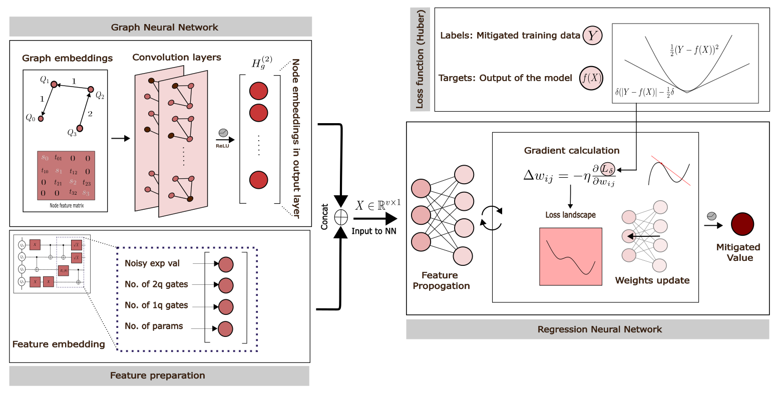
II.3 Machine Learning Model Architecture
We begin this section with the following disclaimer: while in this particular work we generated an ansatz on the fly, the ML model and the associated EM strategy that follow is independent of the way the ansatz is formed and in all aspects, is compatible with any disentangled ansatz. In this section, we give a detailed explanation of how the training data and training labels are generated, how the graph inputs are formulated which serve as an input to GNN, and the working of the entire model along with its complexity.
II.3.1 Graph formulation
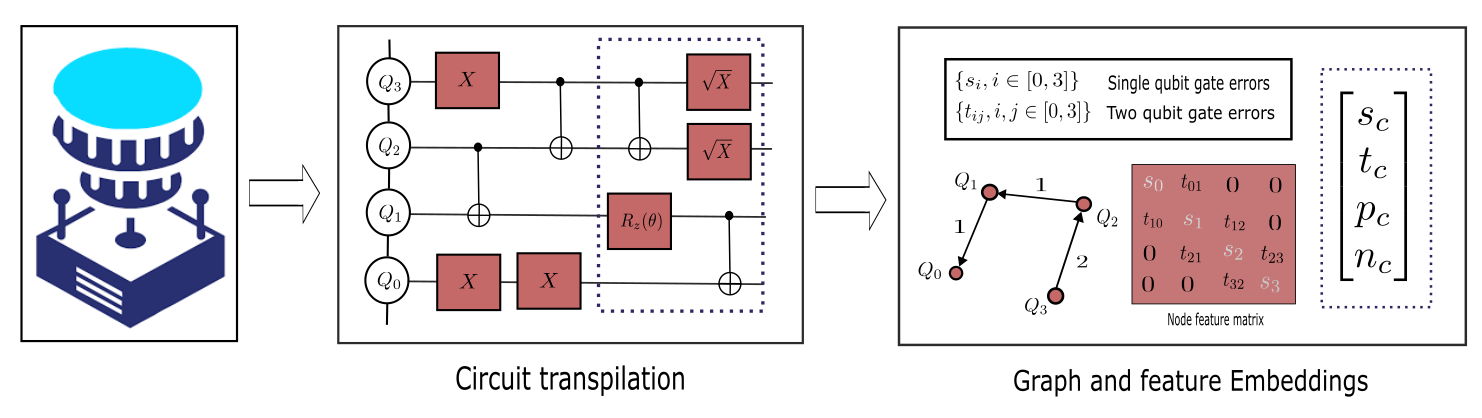
As mentioned in the section I, our training data consists of snippets of circuit ansatz consisting of one- and two-body fermionic excitations which only differ in terms of one and two-qubit gate applications. Therefore, graph representation is a natural modeling choice for such training data and GNNs can elegantly integrate such data structures. As mentioned in the section II.2, we derive the graph by transpiling the circuit adhering to the qubit-connectivity of the real quantum device having number of qubits. Graphs contain two types of information that we may wish to utilize for making predictions: nodes and edge connectivity. The node information can be embedded in the node feature matrix . Expressing the graph’s connectivity is not that straightforward. Using an adjacency matrix might be the most straightforward option, as it can be easily converted into a tensor format. Here we explain how the graph and its corresponding attributes are constructed.
The graph is represented as follows: The nodes correspond to the number of qubits in the device, and directed edges symbolize the CNOT connectivity between the -th (parent node) and -th (target node). The edge weights represent the frequency of identical edges. Subsequently, the matrix is created to incorporate self-loops ( is the identity matrix). The degree matrix is derived from to account for next-neighboring nodes. with . normalizes the adjacency matrix to incorporate information from neighboring nodes.
The feature matrix (g stands for GNN) of the nodes is then constructed. The diagonal elements encode information about single-qubit gate errors specific to each qubit in the hardware used in the circuit. This information encompasses all single-qubit errors associated with the native gates. The off-diagonal elements portray errors in two-qubit CNOT gates concerning the coupling map. The coupling map is a reflection of the physical connectivity of qubits in the hardware. The adjacency matrix represents CNOT connectivity with representing the edge weight between two nodes and . For more details, refer to Fig. 1. The adjacency matrix representation suffers from drawbacks like redundancy and memory issues. One elegant and compact way to represent such sparse matrices is the adjacency list. It represents the connectivity of -th edge as a tuple in the -th entry of the list. For instance, the adjacency list of the graph in Fig. 1 is given as .
II.3.2 GraphNetMitigator Architecture and Training Details
In this section, we describe the GNM architecture developed for error mitigation. We use a Graph Convolutional Network (GCN) to learn the features of the graph where each node corresponds to an dimensional embedding. Once we get the feature matrix and adjacency list of the graph, this input is passed to the GCN which transforms with the following propagation rule for -th layer:
| (7) |
Where is a feature transformation/weight matrix which maps the node features of size to size . The GCN contains two convolutional layers. The first layer has input channels reflecting the number of qubits present in the hardware and output channels and the second layer has input channels and output channel (This flow indicates the node feature transformation from dimension ). When the first layer is applied to the input , it transforms in a way with the weight matrix as shown below. A ReLU activation function is applied on top of it.
Where . This represents the node representations after the first layer of the GCN. After passing through the second layer with a weight matrix of we get,
Where . represents the node representations after the second layer of the GCN. This transformation corresponds to one-dimensional node embedding and serves as an input to our regressor along with additional features.
 |
We construct the rest of the features from the following data set: noisy expectation values learnt over the snippet circuits, number of two-qubit gates, number of single-qubit gates, number of variational parameters (number of single and double excitation operators). We construct a feature vector ( stands for regression) where is the number of features in regressor. is then concatenated with to get final feature vector where . The quantity serves as an input to the feed-forward neural network with one hidden layer of = 64 nodes which is used for the regression task to mitigate the noisy value. First, transforms as follows:
| (9) |
and are weights and biases applied to the input layer with ReLU activation. Hidden layer also transforms in a similar manner giving the mitigated expectation values as output:
| (10) |
The loss function used to calculate the loss is Huber loss. The Huber loss function is often used in regression problems as a combination of the mean squared error and mean absolute error which is defined as:
 |
| (11) |
Where is the mitigated prediction and is the ideal/SREM value (from the snippets) used as a target to calculate the loss. Here is a hyper-parameter determining where the loss transitions from quadratic to linear behavior. In our case, is defined by analyzing the mean square error between ideal/SREM values of the snippets and the corresponding noisy expectation values and for indicating 1, 2, 3-parameter snippet circuits from the training set to handle the outliers. The choice of the loss function is based on the fact that with a given circuit, sampling cost scales exponentially with respect to its depth implying eventual intractability in mitigating associated errors[36]. Giving less weightage to such non-shallow circuit expectation values which show large deviation when SREM values are used as labels or when ideal values are used as labels ensures the proper handling of outliers.
II.3.3 Complexity analysis of the model
Time and Space complexity of GCN: For matrices and , matrix multiplication has a time complexity of . We use pytorch geometric to implement the GCN. PyTorch Geometric first computes the matrix multiplication of of and . To compute , they use coordinate form edge index matrix of size and store the normalization coefficient in a separate matrix called norm. The computation of is what involves the so-called "message passing" and aggregation. So it’s done in a two-step process. The first step is a dense matrix multiplication between matrices of size and . So the time complexity becomes . The second step matrix multiplication of and will have a similar time complexity. In practice, it is computed using a sparse operator, such as the PyTorch scatter function. The activation is simply an element-wise function with a complexity. Considering the neighborhood aggregation of each node, over layers the total time complexity becomes . Backward pass also has a similar time complexity of . More details can be found in [37]. The overall time and space complexity of the GCN model is described in the table below:
Time and Space complexity of Regressor: The regressor uses a simple feed-forward neural network given by the Eq. 9 and Eq. 10. The matrix multiplication of and has a time complexity of = . Adding the activation layer leads to the total time complexity of for layers.
| Algorithm | Time Complexity |
|---|---|
| GCN forward pass | |
| GCN backward pass | |
| Regressor forward pass | |
| Regressor backward pass |
III Results and Discussions:
To demonstrate the working of the GNM (shown in Fig. 2), we test it on two different molecules and two different devices with diverse noise profiles. Since the model is not based on the variational principle, the estimated expectation value can go below the ideal value. With the advent of modern gate error suppression techniques, such as dynamic decoupling and gate twirling, fluctuations in measurement can be greatly suppressed. In a simulation protocol, this can be approximated by using a fixed seed value to represent an averaged sampling statistics which we have chosen to use throughout this work. In this architecture, we train an ML model with circuits composed of single and double excitations to predict noiseless expectation values using noisy ones. The GNM model is developed using PyTorch[38] and PyTorch Geometric. For GNN, we use Graph Convolution Networks. The details of graph encoding and feature construction are found in the Methodology section. In the training data, labels are generated sequentially using the reference error mitigation strategy which uses VQE as a subroutine and is implemented using Qiskit- Nature[39]. The one- and two-body integrals are imported from PySCF[40]. The second-quantized fermionic operators are transformed into qubit operators by using Jordan-Wigner encoding[41]. All the noise models used are derived from fake IBM Quantum hardware. We mainly use noise models imported from fake backends of two quantum devices: ibmq Melbourne and ibmq Guadalupe having 14 and 16 qubits respectively. The model is trained separately for each bond length using the Adam optimizer with 100 epochs. Due to a limited number of data in the training set, batch size is taken as 1.
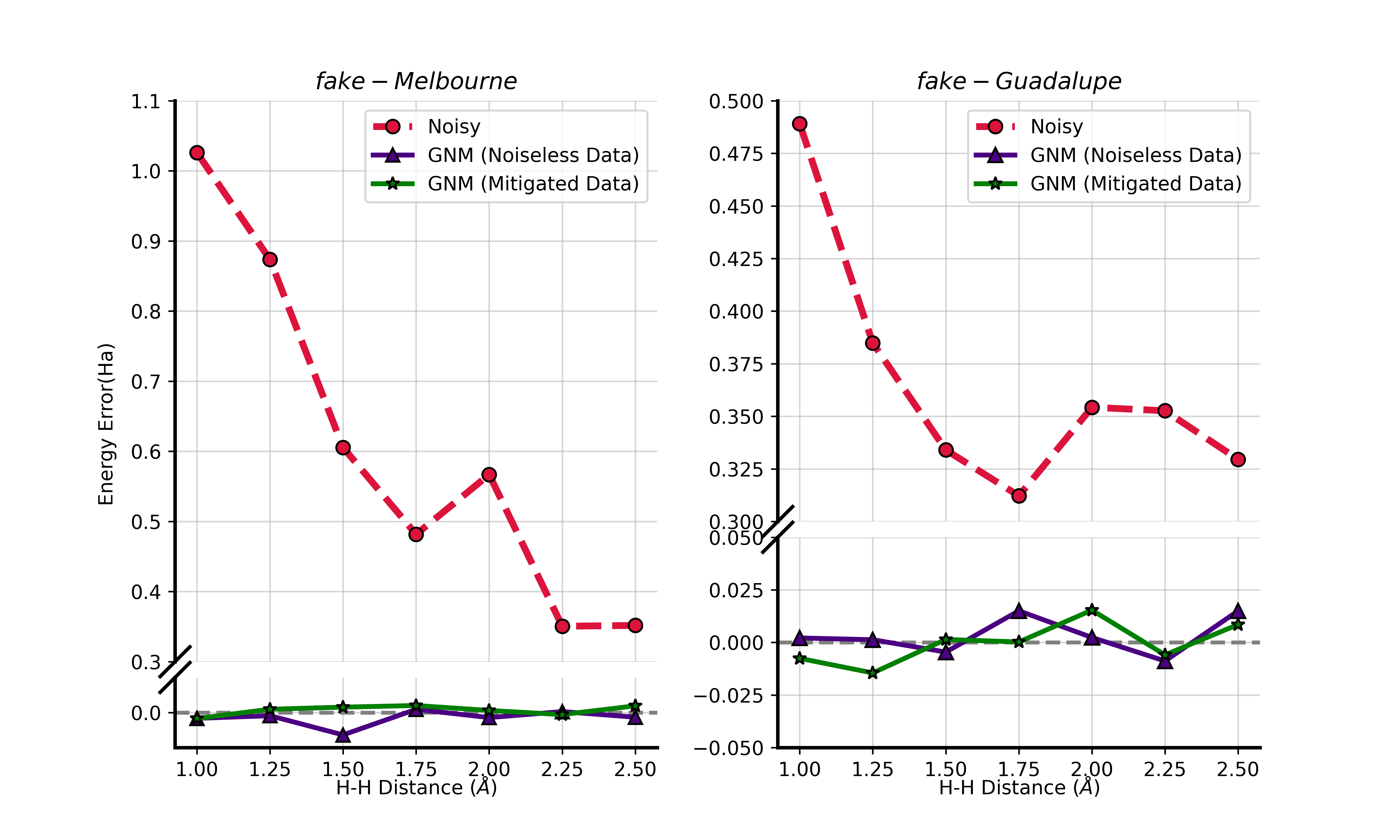
To illustrate the functionality of the GNM, our initial testing focuses on the molecule where we symmetrically stretch all the bonds. In STO-3G basis has 4 electrons in 8 spin-orbitals. From the findings depicted in Fig. 3, it becomes evident that the optimized energy difference for full circuit between the noisy and corresponding noiseless scenarios ranges from approximately 1 to 0.32 on the ibmq-Melbourne machine and from 0.48 to 0.3 on the ibmq-Guadalupe machine. However, when considering the mitigated energy compared to the noiseless energy, the difference is confined within 12 on the ibmq-Melbourne machine when the GNM model is trained with either the noiseless (simulator generated) or SREM training datasets of the snippets. Similarly, on the ibmq-Guadalupe machines, the maximum observed error for GNM mitigated energy reaches around 20 for both the noiseless and SREM training datasets generated from the snippets.
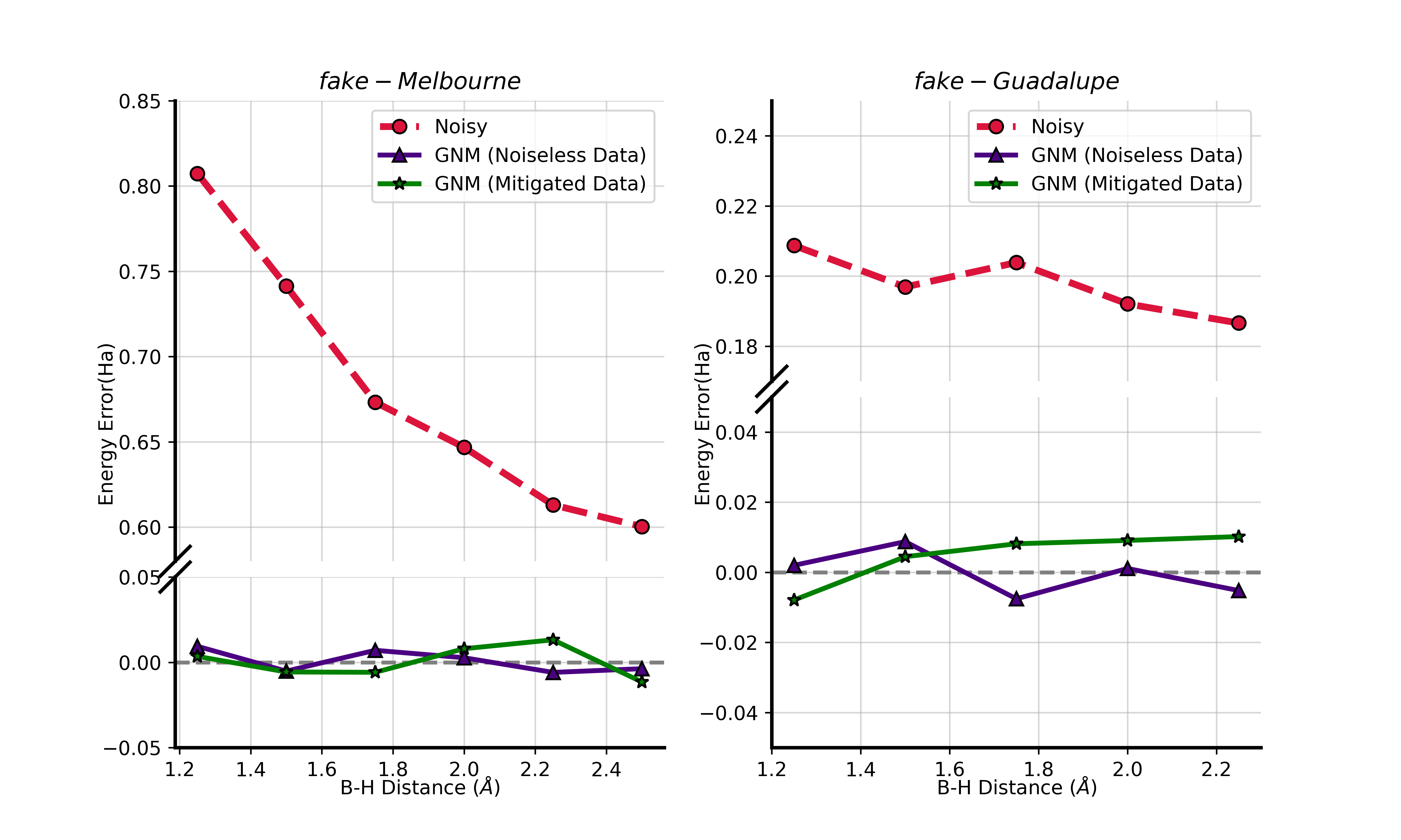
The stretching of the bond represents one of the most challenging test cases for NISQ implementations. In STO-3G basis with frozen 1s core orbital of , it turns out to be a system of 4 electrons in 10 spin-orbitals. Observing Figure 4, it becomes evident that the energy error between the noisy and noiseless scenarios for full circuit fall within the range of 0.82 to 0.59 on fake-ibmq-Melbourne device, and within 0.21 to 0.19 on the fake-ibmq- Guadalupe device. In contrast, the GNM model predicts the mitigated energies which are within 20 and 18 (at max over the potential energy surface, with respect to the corresponding noiseless values) on fake-ibmq-Melbourne and fake-ibmq-Guadalupe machine respectively, irrespective of the training dataset used for the snippets.
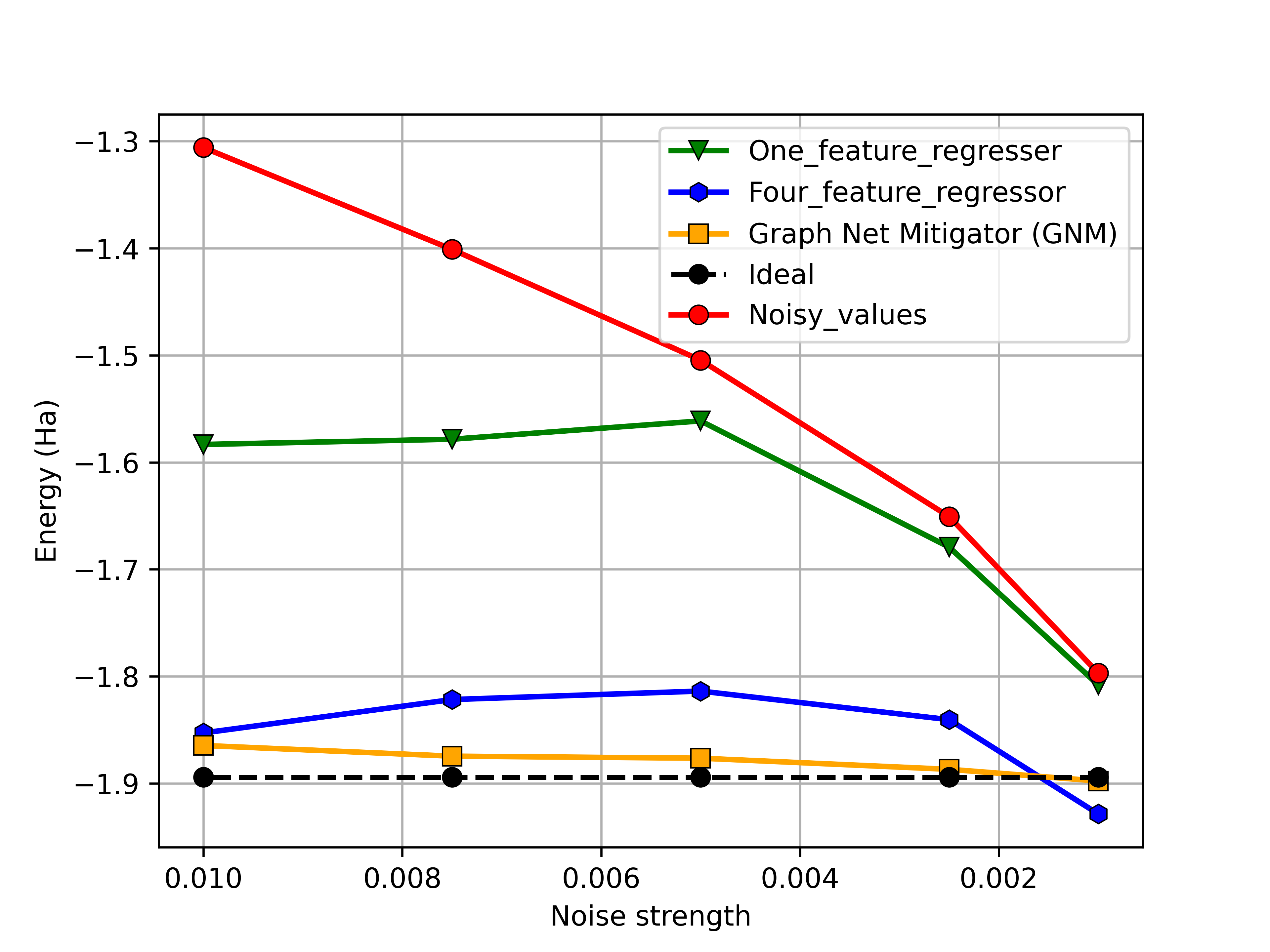
We also tested the robustness of our model against varying noise levels for at 2Å. For this particular analysis, we specifically accounted for the depolarizing noise (which is one of the primary sources of noise in NISQ hardware) with noise strength varying from {0.0001, 0.001} to {0.001, 0.01} for one-qubit and two-qubit gates, respectively. Here the training labels are generated via the SREM mitigated values. The results are shown in Fig. 5. We test for different variations of machine learning models, from only one-feature regression to GNM and in all occasions, GNM predicts the most accurate energy, establishing its robustness across a spectrum of noise strengths. It is particularly interesting to note that with the decrease in noise strength, as expected with the improvement of the hardware quality, GNM predicted values linearly approach the corresponding ’exact’ value, demonstrating its ability to handle the spectrum of noise strength. without overestimating or underestimating. Despite its good performance with some of the most dominant noise channels as discussed so far, its robustness is subject to further validation when the state preparation and measurement (SPAM) errors, without sampling noise suppression models[14, 42], are accounted for. In principle, a separate SPAM error mitigation strategy may be complemented as an additional mitigation layer for better state preparation. However, the current graph network-based model gives us a practical tool to mitigate gate errors that otherwise incur exponential overheads and deep mitigation circuits.
IV Conclusions and Future Outlook
In this work, we developed a learning-based error mitigation technique to accurately predict the ground state energy of molecular Hamiltonian. The developed GNM model successfully predicts the ground state energy of the many-electron Hamiltonian without the need for any additional mitigation circuits and bypasses exponential overhead. GNM outperforms current EM methods like digital-ZNE and PEC which fail at larger and complex circuits. Unlike other NN-based techniques which often use ideal expectation values generated on the simulator as labels, we generate our labels, either by ideal values or by sequentially mitigating the reference error over much shallower snippet circuits, thus eliminating the need to access the ideal quantum computer. The data for training the model is generated on the fly while the ansatz is constructed in a noisy quantum environment. GNM is entirely general mitigation model, and does not have any specific dependence to the underlying ansatz. Our results consistently demonstrate the robustness and effectiveness of GNM across hardware connectivity and a spectrum of synthetic noise strengths, and thus GNM is expected to hold its ground when the qubit quality improves over the coming years.
One important future research direction is the generalization of the model across diverse and larger classes of Hamiltonians and ansatze. Testing the model while considering different noise channels with nonlinear sampling complexity is an important future direction towards establishing its robustness. More importantly, feature selection can be improved using a different set of features altogether. The current method captures the device characteristics through a CNOT-connectivity graph adhering to the coupling map of the device and gate errors. An additional set of features like decoherence time of qubits and other device-specific parameters can be incorporated to further capture the noise profile accurately.
Software
The current model supports Qiskit SDK and is developed using Torch and Torch-Geometric. For mitigation purposes, we use AerEstimator to calculate the noisy values and subsequently mitigated SREM values. We provide detailed documentation and source code of training data generation through SREM and GraphNetMitigator model at https://github.com/Next-di-mension/GraphNetErrorMitigator
Supplementary Material
See supplementary material for the Sequential Reference Error Mitigation (SREM) strategy and the distribution of the all the noisy and REM mitigated energies for two representative molecules in two extreme geometries that were used for label generation.
Acknowledgements
S.P. Thanks to the Industrial Research and Consultancy Center (IRCC), IIT Bombay. S.P. is also thankful to Ananyapam De (Claushtal University of Technology, Germany) for useful discussions on developing the ML model. D.M. acknowledges the Prime Ministers Research Fellowship (PMRF), Government of India for their research fellowships. R.M. acknowledges the financial support from the Anusandhan National Research Foundation (ANRF) (erstwhile SERB), Government of India (Grant Number: MTR/2023/001306).
Conflict of Interests
The authors have no conflict of interest to disclose.
Data Availability
The data that support the findings of this study are available from the corresponding author upon reasonable request.
References
- Abrams and Lloyd [1999] D. S. Abrams and S. Lloyd, “Quantum algorithm providing exponential speed increase for finding eigenvalues and eigenvectors,” Phys. Rev. Lett. 83, 5162–5165 (1999).
- McArdle et al. [2020] S. McArdle, S. Endo, A. Aspuru-Guzik, S. C. Benjamin, and X. Yuan, “Quantum computational chemistry,” Rev. Mod. Phys. 92, 015003 (2020).
- O’Gorman et al. [2022] B. O’Gorman, S. Irani, J. Whitfield, and B. Fefferman, “Intractability of electronic structure in a fixed basis,” PRX Quantum 3, 020322 (2022).
- Colless et al. [2018] J. I. Colless, V. V. Ramasesh, D. Dahlen, M. S. Blok, M. E. Kimchi-Schwartz, J. R. McClean, J. Carter, W. A. de Jong, and I. Siddiqi, “Computation of molecular spectra on a quantum processor with an error-resilient algorithm,” Phys. Rev. X 8, 011021 (2018).
- Hempel et al. [2018] C. Hempel, C. Maier, J. Romero, J. McClean, T. Monz, H. Shen, P. Jurcevic, B. P. Lanyon, P. Love, R. Babbush, A. Aspuru-Guzik, R. Blatt, and C. F. Roos, “Quantum chemistry calculations on a trapped-ion quantum simulator,” Phys. Rev. X 8, 031022 (2018).
- Peruzzo et al. [2014] A. Peruzzo, J. McClean, P. Shadbolt, M.-H. Yung, X.-Q. Zhou, P. J. Love, A. Aspuru-Guzik, and J. L. O’brien, “A variational eigenvalue solver on a photonic quantum processor,” Nature communications 5, 4213 (2014).
- Kandala et al. [2017] A. Kandala, A. Mezzacapo, K. Temme, M. Takita, M. Brink, J. M. Chow, and J. M. Gambetta, “Hardware-efficient variational quantum eigensolver for small molecules and quantum magnets,” nature 549, 242–246 (2017).
- Anand et al. [2022] A. Anand, P. Schleich, S. Alperin-Lea, P. W. K. Jensen, S. Sim, M. Díaz-Tinoco, J. S. Kottmann, M. Degroote, A. F. Izmaylov, and A. Aspuru-Guzik, “A quantum computing view on unitary coupled cluster theory,” Chem. Soc. Rev. 51, 1659–1684 (2022).
- Tilly et al. [2022] J. Tilly, H. Chen, S. Cao, D. Picozzi, K. Setia, Y. Li, E. Grant, L. Wossnig, I. Rungger, G. H. Booth, and J. Tennyson, “The variational quantum eigensolver: A review of methods and best practices,” Phys. Rep. 986, 1–128 (2022).
- Evangelista, Chan, and Scuseria [2019] F. A. Evangelista, G. K.-L. Chan, and G. E. Scuseria, “Exact parameterization of fermionic wave functions via unitary coupled cluster theory,” The Journal of Chemical Physics 151, 244112 (2019), https://pubs.aip.org/aip/jcp/article-pdf/doi/10.1063/1.5133059/16659468/244112_1_online.pdf .
- Wecker, Hastings, and Troyer [2015] D. Wecker, M. B. Hastings, and M. Troyer, “Progress towards practical quantum variational algorithms,” Phys. Rev. A 92, 042303 (2015).
- Temme, Bravyi, and Gambetta [2017] K. Temme, S. Bravyi, and J. M. Gambetta, “Error mitigation for short-depth quantum circuits,” Physical review letters 119, 180509 (2017).
- Khodjasteh and Lidar [2005] K. Khodjasteh and D. A. Lidar, “Fault-tolerant quantum dynamical decoupling,” Phys. Rev. Lett. 95, 180501 (2005).
- Ezzell et al. [2023] N. Ezzell, B. Pokharel, L. Tewala, G. Quiroz, and D. A. Lidar, “Dynamical decoupling for superconducting qubits: A performance survey,” Phys. Rev. Appl. 20, 064027 (2023).
- Van Den Berg et al. [2023] E. Van Den Berg, Z. K. Minev, A. Kandala, and K. Temme, “Probabilistic error cancellation with sparse pauli–lindblad models on noisy quantum processors,” Nature Physics 19, 1116–1121 (2023).
- Stair and Evangelista [2021] N. H. Stair and F. A. Evangelista, “Simulating many-body systems with a projective quantum eigensolver,” PRX Quantum 2, 030301 (2021).
- Halder, Shrikhande, and Maitra [2023] S. Halder, C. Shrikhande, and R. Maitra, “Development of zero-noise extrapolated projective quantum algorithm for accurate evaluation of molecular energetics in noisy quantum devices,” The Journal of Chemical Physics 159, 114115 (2023).
- Kim, Park, and Rhee [2020] C. Kim, K. D. Park, and J.-K. Rhee, “Quantum error mitigation with artificial neural network,” IEEE Access 8, 188853–188860 (2020).
- Bennewitz et al. [2022] E. R. Bennewitz, F. Hopfmueller, B. Kulchytskyy, J. Carrasquilla, and P. Ronagh, “Neural error mitigation of near-term quantum simulations,” Nature Machine Intelligence 4, 618–624 (2022).
- Kim et al. [2022] J. Kim, B. Oh, Y. Chong, E. Hwang, and D. K. Park, “Quantum readout error mitigation via deep learning,” New Journal of Physics 24, 073009 (2022).
- Saravanan and Saeed [2022] V. Saravanan and S. M. Saeed, “Graph neural networks for idling error mitigation,” in Proceedings of the 41st IEEE/ACM International Conference on Computer-Aided Design (2022) pp. 1–9.
- Liao et al. [2023] H. Liao, D. S. Wang, I. Sitdikov, C. Salcedo, A. Seif, and Z. K. Minev, “Machine learning for practical quantum error mitigation,” (2023), arXiv:2309.17368 [quant-ph] .
- Czarnik et al. [2021] P. Czarnik, A. Arrasmith, P. J. Coles, and L. Cincio, “Error mitigation with Clifford quantum-circuit data,” Quantum 5, 592 (2021).
- Quek et al. [2023] Y. Quek, D. S. França, S. Khatri, J. J. Meyer, and J. Eisert, “Exponentially tighter bounds on limitations of quantum error mitigation,” (2023), arXiv:2210.11505 [quant-ph] .
- Takagi, Tajima, and Gu [2023] R. Takagi, H. Tajima, and M. Gu, “Universal sampling lower bounds for quantum error mitigation,” Phys. Rev. Lett. 131, 210602 (2023).
- Yordanov, Arvidsson-Shukur, and Barnes [2020] Y. S. Yordanov, D. R. M. Arvidsson-Shukur, and C. H. W. Barnes, “Efficient quantum circuits for quantum computational chemistry,” Physical Review A 102 (2020), 10.1103/physreva.102.062612.
- Magoulas and Evangelista [2023] I. Magoulas and F. A. Evangelista, “Cnot-efficient circuits for arbitrary rank many-body fermionic and qubit excitations,” Journal of Chemical Theory and Computation 19, 822–836 (2023), pMID: 36656643, https://doi.org/10.1021/acs.jctc.2c01016 .
- Grimsley et al. [2019] H. R. Grimsley, S. E. Economou, E. Barnes, and N. J. Mayhall, “An adaptive variational algorithm for exact molecular simulations on a quantum computer,” Nat. Commun. 10, 3007 (2019).
- Lee et al. [2018] J. Lee, W. J. Huggins, M. Head-Gordon, and K. B. Whaley, “Generalized unitary coupled cluster wave functions for quantum computation,” J. Chem. Theory Comput. 15, 311–324 (2018).
- Mondal et al. [2023] D. Mondal, D. Halder, S. Halder, and R. Maitra, “Development of a compact Ansatz via operator commutativity screening: Digital quantum simulation of molecular systems,” The Journal of Chemical Physics 159, 014105 (2023), https://pubs.aip.org/aip/jcp/article-pdf/doi/10.1063/5.0153182/18032301/014105_1_5.0153182.pdf .
- Halder, Mondal, and Maitra [2024] D. Halder, D. Mondal, and R. Maitra, “Noise-independent route toward the genesis of a COMPACT ansatz for molecular energetics: A dynamic approach,” The Journal of Chemical Physics 160, 124104 (2024), https://pubs.aip.org/aip/jcp/article-pdf/doi/10.1063/5.0198277/19844810/124104_1_5.0198277.pdf .
- Halder et al. [2024] S. Halder, A. Dey, C. Shrikhande, and R. Maitra, “Machine learning assisted construction of a shallow depth dynamic ansatz for noisy quantum hardware,” Chem. Sci. 15, 3279–3289 (2024).
- Fan et al. [2023] Y. Fan, C. Cao, X. Xu, Z. Li, D. Lv, and M.-H. Yung, “Circuit-depth reduction of unitary-coupled-cluster ansatz by energy sorting,” The Journal of Physical Chemistry Letters 14, 9596–9603 (2023), pMID: 37862387, https://doi.org/10.1021/acs.jpclett.3c01804 .
- Cao et al. [2022] C. Cao, J. Hu, W. Zhang, X. Xu, D. Chen, F. Yu, J. Li, H.-S. Hu, D. Lv, and M.-H. Yung, “Progress toward larger molecular simulation on a quantum computer: Simulating a system with up to 28 qubits accelerated by point-group symmetry,” Phys. Rev. A 105, 062452 (2022).
- Mondal and Maitra [2025] D. Mondal and R. Maitra, “Determination of molecular symmetry adapted eigenroots in the variational quantum eigensolver framework,” International Journal of Quantum Chemistry 125, e70029 (2025), https://onlinelibrary.wiley.com/doi/pdf/10.1002/qua.70029 .
- Takagi et al. [2022] R. Takagi, S. Endo, S. Minagawa, and M. Gu, “Fundamental limits of quantum error mitigation,” npj Quantum Information 8, 114 (2022).
- Blakely, Lanchantin, and Qi [2021] D. Blakely, J. Lanchantin, and Y. Qi, “Time and space complexity of graph convolutional networks,” Accessed on: Dec 31, 2021 (2021).
- Paszke et al. [2019] A. Paszke, S. Gross, F. Massa, A. Lerer, J. Bradbury, G. Chanan, T. Killeen, Z. Lin, N. Gimelshein, L. Antiga, A. Desmaison, A. Köpf, E. Yang, Z. DeVito, M. Raison, A. Tejani, S. Chilamkurthy, B. Steiner, L. Fang, J. Bai, and S. Chintala, “Pytorch: An imperative style, high-performance deep learning library,” (2019), arXiv:1912.01703 [cs.LG] .
- developers and contributors [2023] T. Q. N. developers and contributors, “Qiskit nature 0.6.0,” (2023).
- Sun et al. [2018] Q. Sun, T. C. Berkelbach, N. S. Blunt, G. H. Booth, S. Guo, Z. Li, J. Liu, J. D. McClain, E. R. Sayfutyarova, S. Sharma, S. Wouters, and G. K.-L. Chan, “Pyscf: the python-based simulations of chemistry framework,” WIREs Comput. Mol. Sci. 8, e1340 (2018).
- Seeley, Richard, and Love [2012] J. T. Seeley, M. J. Richard, and P. J. Love, “The bravyi-kitaev transformation for quantum computation of electronic structure,” J. Chem. Phys. 137, 224109 (2012).
- Wallman and Emerson [2016] J. J. Wallman and J. Emerson, “Noise tailoring for scalable quantum computation via randomized compiling,” Phys. Rev. A 94, 052325 (2016).