Universal neural wave functions for high-pressure hydrogen

Abstract

We leverage the power of neural quantum states to describe the ground state wave function of solid and liquid dense hydrogen, including both electronic and protonic degrees of freedom. For static protons, the resulting Born-Oppenheimer energies are consistently lower than all previous projector Monte Carlo calculations for systems containing up to $128$ hydrogen atoms. In contrast to conventional methods, we introduce a universal trial wave function whose variational parameters are optimized simultaneously over a large set of proton configurations spanning a wide pressure-temperature spectrum and covering both molecular and atomic phases. This global optimization not only yields lower energies compared to benchmarks but also brings an enormous reduction in computational cost. By including nuclear quantum effects in the zero-temperature ground state, thus going beyond the Born-Oppenheimer approximation, our description overcomes major limitations of current wave functions, notably by avoiding any explicit symmetry assumption on the expected quantum crystal and sidestepping efficiency issues of imaginary time evolution with disparate mass scales. As a first application, we examine crystal formation in an extremely high-density region where pressure-induced melting is expected.

Introduction–

Atomic and molecular hydrogen have played a fundamental role in the development of quantum mechanics and quantum chemistry. High-pressure experiments have revealed the existence of several unexpected molecular solid phases [1, 2] in the long-lasting search for atomic metallic hydrogen [3]. Despite the apparent simplicity, understanding the properties of high-pressure hydrogen and deuterium remains a formidable challenge for advanced first-principle simulation methods [4, 5].

Diffusion Monte Carlo (DMC) calculations [6] have provided some of the most accurate zero-temperature descriptions. However, hydrogen simulations remain challenging for two main reasons. First, the fixed-node approximation—inherent to DMC and required to resolve the fermion sign problem—relies on trial wave functions of exceptional accuracy to capture the subtle physics of high-pressure phases. Second, the very large proton-to-electron mass ratio ($m_{p}/m_{e}\simeq 1836$) requires long projection times in imaginary time evolution, substantially increasing the computational cost. These difficulties are compounded in related methods like reptation Monte Carlo (RMC) and finite-temperature path integral Monte Carlo (PIMC) [7, 8].

In this work, we show that Variational Monte Carlo (VMC) with neural quantum states (NQS) overcomes these limitations by employing a flexible backflow wave function—enhanced through a graph neural network that couples electrons and protons—and globally optimizing its parameters over a diverse set of proton configurations. The associated universal ansatz, akin to recent foundation models for wave functions [9, 10, 11], spans a wide pressure–temperature range, capturing both molecular and atomic phases, and yields energies below DMC benchmarks with orders-of-magnitude computational savings. By naturally including nuclear quantum effects beyond the traditional Born–Oppenheimer approximation (BOA), our method avoids ad hoc symmetry constraints, which is essential for exploring high-pressure hydrogen phases where crystalline structures are unknown and conventional methods falter due to mass-scale disparities. As a first application, we study the onset of crystal formation in an ultra-dense region where pressure-induced melting is expected.

Since the first quantum Monte Carlo (QMC) studies on hydrogen [6, 12], only a few works have treated electronic and protonic degrees of freedom on equal footing [13, 14, 15]. Advances in QMC stem from decoupling electronic and protonic motions within the BOA. This underlies coupled electron ion Monte Carlo (CEIMC) [16] and ab-initio molecular dynamics (MD) [17] methods, operating at temperatures substantially below the electronic Fermi temperature, but high enough to describe nuclear motion within the adiabatic approximation (i.e. the BOA). Within the BOA, robust QMC trial wave functions are built from Hartree-Fock or density functional theory (DFT) band structure methods [18, 13, 14, 19], and improved with backflow coordinates [20]. The nuclear motion is then obtained via MD or PIMC [21, 4, 22] with recent deep network free energy methods [23, 24].

Benchmarking our NQS on static proton configurations, for instance from the Dense hydrogen DMC database [25, 26], we obtain BO energies that surpass DMC accuracy. This demonstrates the flexibility of backflow-based NQS for high-pressure hydrogen, as seen in studies of other systems such as atoms and molecules [27, 28, 29, 30, 11, 10, 31, 32, 33], as well as electron matter [34, 35, 36, 37, 38, 39, 40]. Moreover, our network serves as a fully transferable foundation model for extended hydrogen.

We then address the full Schrödinger equation for electrons and protons—the “dynamic” case—thereby going beyond the BOA. Unlike BO wave functions with orbitals tied to a fixed proton configuration, our NQS explicitly incorporates proton motion via a factor capturing zero-point motion. Our ansatz accurately describes liquid and solid phases in a translationally invariant form, without imposing a particular crystal symmetry [41, 42], which is crucial for high-pressure hydrogen where the phase diagram is not fully determined. Unlike DMC methods, burdened by fixed crystalline assumptions and mass-dependent convergence issues [43], the convergence of our VMC approach does not depend on the nuclear mass. Finally, we present preliminary results in the region where atomic hydrogen is expected to melt at ultra-high pressures.

Method–

We consider $N$ hydrogen atoms in a simulation cell of volume $V=4\pi Nr_{s}^{3}a_{0}^{3}/3$, where $r_{s}=a/a_{0}$ parametrizes the electronic number density, with $a$ and $a_{0}$ being the mean electronic distance and the Bohr radius, respectively. To simplify the notation, we will consider only the case of a cubic box of extension $L=V^{1/3}$ in the following. We denote the electron and proton coordinates by $\{\mathbf{r}_{i}\}$ and $\{\mathbf{R}_{I}\}$, respectively. As we simultaneously sample both sets of coordinates using Monte Carlo, a configuration is denoted $\mathbf{X}\equiv\{\mathbf{r},\mathbf{R}\}\equiv\{\mathbf{r}_{1},\ldots,\mathbf{r}_{N},\mathbf{R}_{1},\ldots,\mathbf{R}_{N}\}$. We periodize the simulation cell so that the Hamiltonian in atomic units reads

$$H=-\sum_{a=1}^{2N}\frac{1}{2m_{a}}\nabla_{\mathbf{x}_{a}}^{2}+\frac{1}{2}\sum_{\mathbf{n\in\mathbb{Z}^{3}}}\sum_{a,b=1}^{2N}{}^{\hskip-2.84526pt{}^{\prime}}\frac{q_{a}q_{b}}{|\mathbf{x}_{a}-\mathbf{x}_{b}+\mathbf{n}L|},$$ (1)

where $\mathbf{x}_{a}\in\mathbf{X}$, $m_{a}$ and $q_{a}$ are respectively the mass and electric charge of particle $a$. The restriction on the Coulomb sum, denoted by an apostrophe, specifies that $\mathbf{n}=\mathbf{0}$ is omitted when $a=b$. The Ewald procedure [44] is used to evaluate the (conditionally convergent) second term in Eq.˜1.

To construct a ground state trial wave function, it is convenient to consider the following general form

$$\Psi(\mathbf{X})=\Phi(\mathbf{R})\mathrm{det}[\phi_{a}(\mathbf{r}_{i}|\mathbf{X})]e^{-U(\mathbf{X})},$$ (2)

where $U(\mathbf{X})$ denotes a symmetric correlation factor, $\Phi(\mathbf{R})$ is a pure nuclear wave function, and $\{\phi_{a}(\mathbf{r}_{i}|\mathbf{X})\}$ is a set of electronic orbitals, with $1\leq a\leq N$, which may symmetrically depend on all coordinates in $\mathbf{X}$ that are different from $\mathbf{r}_{i}$. Although this form is general for all fermionic ground state wave functions [45, 46, 47], there is no guarantee that the orbitals $\phi_{a}(\mathbf{r}_{i}|\mathbf{X})$ can be efficiently represented numerically.

In the first calculations on dense hydrogen [6, 12], $U(\mathbf{X})$ was chosen as a sum of pairwise correlation factors in terms of electron-electron (e-e), electron-proton (e-p) and proton-proton (p-p) pseudo-potentials. The orbital part of the wave function consisted of Slater determinants for spin-up and spin-down electrons occupying either plane wave orbitals with wavevectors $\mathbf{k}$ below the Fermi surface, or Gaussians localized at the crystalline lattice sites $\{\mathbf{R}_{I}^{(0)}\}$. Later calculations [14] have used orbitals from DFT within the local-density approximation (LDA), with the orbitals also pinned at $\{\mathbf{R}_{I}^{(0)}\}$. Exchange effects for protons (and deuterium) are expected to be small in the crystalline phase [6]. Quantum statistical effects on protons have thus been neglected, and the proton crystal was described by the asymmetric (Nosanow) wave function $\Phi(\mathbf{R})=\prod_{I}\varphi(|\mathbf{R}_{I}-\mathbf{R}_{I}^{(0)}|)$ [48, 49], where $\varphi$ is a Gaussian function with a width variational parameter to optimize. Although DMC stochastically improves the wave function via imaginary time projection, in practice the results are strongly biased by the explicit dependence on the assumed crystalline structure. Full exploration of the nuclear phase space in imaginary time is difficult due to the large mass imbalance between protons and electrons. We note that the effect is amplified when considering the deuterium having twice the proton’s mass and obeying bosonic nuclear statistics. Backflow and three-body correlations in hydrogen [20] have shown to improve energies also for the fully dynamic protons at zero-temperature [15], but it has not been explored further since.

Our wave function builds upon these previous ones by incorporating two important modifications. First, as electronic orbitals we use

$$\phi_{\mathbf{k}}^{\sigma}(\mathbf{r}_{i})=\sum_{\mathbf{n}\in\mathbb{Z}^{3}}\sum_{I=1}^{N}e^{i\mathbf{k}\cdot(\mathbf{R}_{I}+\mathbf{n}L)}\chi(\mathbf{r}_{i}^{\sigma}-\mathbf{R}_{I}-\mathbf{n}L),$$ (3)

which coincide with Bloch functions for static protons. For $\chi$, we have chosen a Gaussian with a free width parameter. While these radially symmetric s-orbitals seem to be sufficient at describing the range of densities studied in this work, angular dependence via higher orbitals (p, d, f, etc.) can be included in a straightforward manner.

Second, we increase the expressivity of the trial wave function by adding propagator-like backflow to the electron coordinates,

$$\mathbf{r}_{i}\to\mathbf{r}_{i}+W\mathbf{y}_{i}^{(b)},$$ (4)

where $\mathbf{y}_{i}^{(b)}$ is the electron vertex output of a message-passing neural network (MPNN) after $b$ iterations, and $W$ is a matrix of complex variational parameters. This electron backflow is only added in the orbital part of the wave function. For $U(\mathbf{X})$, we take advantage of the electron edge output of the MPNN, denoted $\mathbf{Y}_{ij}^{(b)}$, to create a propagator-like term, similarly as in [42]. With this additional piece the correlation factor $U(\mathbf{X})$ reads

$$U(\mathbf{x})\to U(\mathbf{x})+\sum_{i<j}\left[w\ \mathrm{MLP}(\mathbf{Y}_{ij}^{(b)})\right],$$ (5)

where MLP stands for multilayer perceptron and $w\in\mathbb{R}$ is some variational parameter. The MPNN operates on two underlying graphs: the electron one and the proton one, which interact at each message-passing iteration. In particular, it involves e-e and e-p contributions, meaning that the resulting backflow involve both the electron and proton coordinates, with the e-p contributions capturing a smaller – though important – part of the correlation. Details are provided in the Supplemental Material. This corresponds to a modified version of the message-passing neural quantum state (MP-NQS) architecture introduced in [50]. In the dynamic case, when the protons are not localized to lattice sites, the zero-point motion of the protons is captured with the edge output $\mathbf{Y}_{IJ}^{(b)}$ of a different MPNN than the electronic one, which is processed similarly as in Eq.˜5. This latter MPNN operates only on a single graph – the proton one.

Although we can reach large system sizes of around $10^{2}$ particles with our implementation (see the Results), important finite-size effects remain, which can be addressed from strategies discussed in Ref. [51]. Most important, especially for metallic systems, are shell effects due to the sharp Fermi surface. These shell effects can however be strongly reduced by employing twist-averaged boundary conditions (TABC) [52], which impose the following constraint on the wave function

$$\Psi(\mathbf{r}_{1}+L\mathbf{e}_{\alpha},\ldots,\mathbf{r}_{N},\mathbf{R})=e^{i\theta_{\alpha}}\Psi(\mathbf{r}_{1},\ldots,\mathbf{r}_{N},\mathbf{R}),$$ (6)

where $\mathbf{e}_{\alpha}$ denotes the unit vector in the direction of $\alpha\in\{x,y,z\}$, $-\pi\leq\theta_{\alpha}<\pi$, and it was applied without loss of generality to the first electron coordinate. We remark that we have only imposed TABC on the electronic degrees of freedom. Periodic boundary conditions (PBC) correspond to the special case where the twist angle is trivial, that is $\bm{\theta}\equiv(\theta_{x},\theta_{y},\theta_{z})=\bm{0}$. We can impose TABC on the wave function by selecting the “twisted” wavevector $\mathbf{k}=(2\pi\mathbf{m}+\bm{\theta})/L$, with $\mathbf{m}\in\mathbb{Z}^{3}$, for the electronic orbitals. In practice, the electron orbitals are then filled by taking the twisted wavevectors with the smallest norm.

Global Variational Energy –

Within the static protons framework, we use a global optimization strategy, where a single wave function is used to approximate the electronic ground states corresponding to any arbitrary proton configurations, in principle. To fully capture the coupled electronic and nuclear degrees of freedom within our universal variational ansatz, we compute the expectation value of the Hamiltonian over a large ensemble of proton configurations. Concretely, the global variational energy is given by

$$E_{\mathrm{global}}(\bm{\alpha})=\int d\mathbf{R}\mathcal{P}(\mathbf{R})\frac{\langle\Psi_{\bm{\alpha}}(\mathbf{R})|H_{\mathbf{R}}|\Psi_{\bm{\alpha}}(\mathbf{R})\rangle}{\langle\Psi_{\bm{\alpha}}(\mathbf{R})|\Psi_{\bm{\alpha}}(\mathbf{R})\rangle},$$ (7)

where $\Psi_{\bm{\alpha}}(\mathbf{R})$ denotes the electronic component of the trial wave function corresponding to a particular proton configuration $\mathbf{R}$, and $\mathcal{P}(\mathbf{R})$ is a given probability density for proton configurations. Here, $H_{\mathbf{R}}$ is the BO Hamiltonian evaluated for fixed proton positions $\mathbf{R}$. A single global set of variational parameters, $\bm{\alpha}$, is then optimized over the entire ensemble of proton configurations, ensuring unbiased sampling across different regions of the phase diagram. In essence, this global evaluation approach embodies the key idea behind foundation models, where a universal ansatz is trained on a diverse dataset to achieve both high accuracy and significant computational efficiency. This general global optimization paradigm is discussed for example in Ref. [9], where, importantly, the theoretical framework to generalize the stochastic reconfiguration optimization scheme [53, 54, 55] to multiple auxiliary systems (in this case, labeled by $\mathbf{R}$) is presented. Details on the global optimization procedure are further provided in the End Material.

Results–

$N$	wave function	$E/N$	$\sigma^{2}/N$
16	SJ-PW (DMC)	-0.4857(1)	0.0773(25)
	SJ-LDA (DMC)	-0.4890(5)	-
	BF-PW (DMC)	-0.4905(1)	0.0232(1)
	NQS (VMC)	-0.49154(1)	0.0062(1)
54	SJ-PW (DMC)	-0.5329(1)	0.0642(9)
	BF-PW (DMC)	-0.5382(1)	0.0222(2)
	SJ-LDA (DMC)	-0.5390(5)	-
	NQS (VMC)	-0.54007(2)	0.00479(7)
128	SJ-PW	-0.4900(2)	0.0656(23)
	BF-PW (DMC)	-0.4978(4)	0.030(1)
	SJ-LDA (DMC)	-0.4978(2)	-
	NQS (VMC)	-0.49991(7)	0.00771(4)

Table 1: Static hydrogen with protons pinned to a BCC lattice at $r_{s}=1.31$ using PBC. The energy per atom, $E/N$, is given in units of Hartree, and $\sigma^{2}$ denotes the energy variance. The NQS energy, obtained from VMC calculations using the ansatz given in Eq.˜2, is compared to previous DMC reference energies taken from [20], based on Slater-Jastrow (SJ-PW) and backflow (BF-PW) plane wave orbitals as well as Slater-Jastrow calculations using DFT-LDA (SJ-LDA) orbitals.

As a first step, we want to establish the accuracy of our NQS compared to previous VMC and DMC results. Prior calculations have almost exclusively focused on BOA ground state of electrons using the external (Coulomb) potential of the static protons. Formally, the BOA Hamiltonian corresponds to infinite proton mass in Eq. (1), in which case the protonic coordinates of our wave function, given in Eq.˜2, merely become static parameters. Additional implicit parametric dependence on $\mathbf{R}$ may be introduced via the optimization parameters.

In Table˜1, we compare our results for static protons localized on a perfect body-centered cubic (BCC) lattice around metallization, at $r_{s}=1.31$, with DMC calculations using Slater-Jastrow (SJ) and backflow wave functions with metallic plane wave orbitals [20], as well as with LDA-DFT orbitals [14]. Those calculations have been performed for $N=16$, $54$, and $128$ electrons under PBC. Our VMC results systematically lower the energies per atom by $\sim 1$ mHa compared to the best DMC calculations. The quality of the wave function is further quantified by roughly a fivefold reduction in variance. Notably, about the same improvement is obtained for all three system sizes, illustrating the size consistency of our wave function and of the results. In the Supplemental Material, we further provide explicit comparisons of twist-averaged calculations for static protons in different crystal structures obtained with RMC in Ref. [19], based on backflow wave functions with DFT orbitals, and as used in CEIMC calculations.

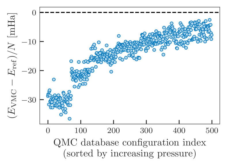
Figure 1: Performance of the NQS on a randomly selected subset of the DMC database [25, 26] configurations, not necessarily included in the training set. The configurations are in a pressure range of $[50,200]$ GPa and a temperature range of $[600,2200]$ K. The trial wave function’s parameters were simultaneously optimized for 1024 different (static) proton configurations from the database, each with a different twist angle. The twist-averaged energy $E_{\mathrm{VMC}}$ of a given configuration is then calculated using these globally optimized parameters and compared to the DMC reference energy, $E_{\text{ref}}$, of the database. The configurations were sorted by increasing pressure from left (lower pressures) to right (higher pressures).

So far, we have shown that our NQS wave function reaches and improves DMC energies by focusing on high-symmetry configurations, which enabled direct comparison with the literature. We now turn to generic proton configurations provided in the dense hydrogen DMC database from Ref. [25, 26]. The database includes molecular-solid and liquid configurations for $N=96$ atoms, spanning a broad pressure-temperature region in the phase diagram, with pressures from 50 to 200 GPa and temperatures from 600 to 2200 K. Here, rather than optimizing our NQS with a single proton configuration at a time, we simultaneously optimize the NQS over many configurations to obtain “global” variational parameters (see Eq. 7, and End Matter for more details), valid over the full pressure-temperature range in the database.

$N$	wave function	$E/N$	$\sigma^{2}/N$
16	SJ-LDA (VMC)	-0.46785(2)	-
	BF-PW (VMC)	-0.4724(1)	0.030(2)
	BF-PW (DMC)	-0.4792(1)	-
	NQS (VMC)	-0.48091(5)	0.0114(1)
54	SJ-LDA (VMC)	-0.5195(2)	-
	SJ-LDA (DMC)	-0.52415(5)	-
	BF-PW (VMC)	-0.52194(5)	0.025(1)
	BF-PW (DMC)	-0.52610(7)	-
	NQS (VMC)	-0.52854(9)	0.0088(1)

Table 2: Ground state energies for dynamic hydrogen at $r_{s}=1.31$, for different wave functions obeying PBC. The reference VMC and DMC energies for Slater-Jastrow with LDA-DFT orbitals (SJ-LDA) and backflow plane wave orbitals (BF-PW) are taken from [15]. For all calculations, the nuclear part of the trial wave function is given by gaussians localized around BCC lattice sites.

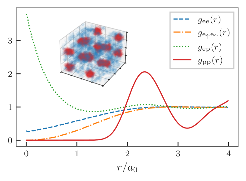
Figure 2: Four pair correlation functions are shown for $N=54$ between three different types of particles: “e”, “p” and “e_↑”, corresponding to electrons, protons and spin-up electrons respectively. An inset with 300 Monte Carlo configurations in the BCC crystal is depicted (for $N=16$, for clarity), where protons form the localized red balls while electrons form the delocalized blue cloud.

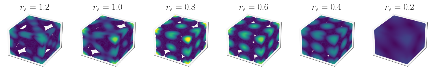
Figure 3: Pair correlation function for $N=8$ protons at different densities under PBC. The same color scale is used in all subplots, globally adjusted with a power law normalization to enhance visibility of the structural features. A fixed threshold is manually set to prevent plotting areas where the pair correlation function has low values. At $r_{s}=0.2$, the structure is drastically reduced suggesting that the system turned liquid.

The configurations used for the global optimization were randomly selected, without biasing a particular region of the phase diagram. Fig.˜1 shows that our NQS reaches in all cases considered the twist-averaged SJ DMC energies of Ref. [25], based on DFT orbitals, and often provides a significant gain in energy. The global variational parameters were optimized for roughly three days on a single NVIDIA H100 GPU. The energy calculations of the 500 proton configurations, shown in Fig.˜1, were performed on configurations that were not necessarily included in the training set, for an additional $\sim$15 hours of runtime on two NVIDIA H100 GPUs. The computational cost savings are substantial compared to DMC, ranging from one to several orders of magnitude (see the End Matter). However, the gain in energy with respect to DMC is decreasing with increasing pressure, suggesting that the SJ nodes, limiting the accuracy of the DMC calculations in Ref. [25], become better when approaching atomic (metallic) states at higher pressure. A more detailed investigation of this pressure bias is beyond the scope of the present paper. We remark that energies can be systematically improved by taking a larger training set, that is, optimizing over a larger number of proton configurations from the database. We further stress that while optimizing for a single proton configuration at a time would also systematically lower the energies, it would be a computationally expensive and inefficient process.

Our results already clearly demonstrate that our ansatz competes with state-of-the-art DMC results both in robustness and computational efficiency, and can be used to improve the electronic part of CEIMC in future work. Furthermore, as an application, in particular to the large scale exploration of the hydrogen phase diagram, energies provided in the benchmark with the dense hydrogen database [25, 26] can be used to improve the precision of machine-learned effective potentials for hydrogen atoms [56, 57, 58, 59, 25, 60, 61, 62] or to benchmark DFT functionals [63, 64].

We finally present the calculations of ground state energies with dynamical protons without relying on the BOA. As a first benchmark, we consider hydrogen at $r_{s}=1.31$, with localized Gaussians for the nuclear wave function $\Phi(\mathbf{R})$, so that the proton positions fluctuate around BCC lattice sites. This allows us to faithfully compare in Table˜2 with VMC and DMC results from Ref. [15], based on BF-PW and SJ-LDA trial wave functions. Again, improvement is consistently obtained. To provide more insights into the structure of the optimized wave function, we further show in Fig.˜2 pair correlation functions between different particle types (electrons, protons and spin-up electrons), as well as Monte Carlo configurations in position space showcasing the BCC lattice structure.

We finally fully relax the nuclear wave function without imposing any crystalline lattice – keeping the wave function fully translationally invariant – and explore the ground state structures of $N=8$ atoms under increasing compression. Fig.˜3 shows the (proton-proton) pair correlation function in three dimensional space, at various pressures near the expected melting transition. The method used is clearly able to find structural changes when increasing the pressure (or lowering $r_{s}$) and the system turns liquid around $r_{s}\approx 0.2$. However, studies at larger system sizes and different cell geometries are required to precisely determine the melting density. So far, pressure-induced melting of hydrogen has only been studied from approximate matching to calculations for the one-component plasma [65], as well as under the approximate Thomas-Fermi screening model that uses a Yukawa pair-potential for the proton-proton interaction [66, 67, 68]. The method presented here – relying on NQS – is promising for identifying and characterizing the expected melting transition.

Although melting occurs at ultra-high densities, the inter-protonic distance $a^{p}$ remains larger than the protonic Bohr radius ($a_{0}^{p}\equiv a_{0}m_{e}/m_{p}$), that is, $a^{p}/a_{0}^{p}\simeq 1836\,r_{s}$. This justifies neglecting fermionic statistics in the solid phase, which means in practice that no protonic determinants are included in the wave function. Inclusion of finite-size effects, by imposing TABC for instance, as well as Fermi statistics for protons and isotope effects, will be addressed in future work.

Conclusion–

We have introduced a neural quantum state (NQS) that accurately describes electron-ion systems, embodying a universal, foundation-model approach. Validated against RMC and DMC results, our method achieves high precision both in the Born–Oppenheimer regime and for the full zero–temperature ground state beyond traditional approximations. Our preliminary study demonstrates that our NQS can capture the zero–temperature melting of atomic hydrogen while treating protons and electrons on equal footing. This universal ansatz not only improves on established QMC methods in accuracy and scalability but also offers orders-of-magnitude computational savings. These attributes pave the way for an extensive exploration of the high–pressure phase diagram—including molecular solids—for both protons and deuterium. Moreover, the incorporation of nuclear quantum statistics opens promising avenues for studying isotope effects and nuclear spin phenomena such as the ortho–para transitions in molecular hydrogen.

End Matter

Global Optimization over Many Proton Configurations –

Our aim is to optimize a single set of variational parameters, $\bm{\alpha}$, so that the electronic ground state wave function $\Psi_{\alpha}(\mathbf{R})$ accurately describes all BO Hamiltonians, $H_{\mathbf{R}}$, associated with different static proton configurations $\mathbf{R}$. In the most general form, the associated global variational energy $E_{\mathrm{global}}(\alpha)$ is given in Eq.˜7. In practice, the integration over $\mathcal{P}(\mathbf{R})$ is performed through Monte Carlo averages obtained using a finite set of $M$ proton configurations i.i.d. from the reference probability distribution, that is, $\mathbf{R}_{I}\sim\mathcal{P}(\mathbf{R}_{I})$. It then takes the following discrete form

$$E_{\mathrm{global}}(\bm{\alpha})=\frac{1}{M}\sum_{I=1}^{M}\frac{\langle\Psi_{\bm{\alpha}}(\mathbf{R}_{I})|H_{\mathbf{R}_{I}}|\Psi_{\bm{\alpha}}(\mathbf{R}_{I})\rangle}{\langle\Psi_{\bm{\alpha}}(\mathbf{R}_{I})|\Psi_{\bm{\alpha}}(\mathbf{R}_{I})\rangle}.$$ (8)

In this work, we consider proton configurations re-sampled uniformly from an existing dataset of configurations, $\mathcal{D}$. A uniform distribution $\mathcal{P}(\mathbf{R})=1/M$ is therefore implicitly assumed in Eq.˜8, with $\mathbf{R}_{I}\in\mathcal{D}$. We consider $M=17\,528$ configurations from the Dense hydrogen DMC database [25, 26]—spanning pressures from 50 to 200 GPa and temperatures from 600 to 2200 K. This global optimization contrasts sharply with the conventional approach of individually optimizing the electronic wave function for each proton configuration. Although the latter might yield marginal energy gains, it is exceedingly inefficient and requires extensive computational resources and human intervention.

In our procedure, a training set of 1024 configurations is randomly selected from the database (without bias toward any pressure or temperature region), and $\bm{\alpha}^{*}$ is obtained by minimizing Eq. (7) over this set. A test set is then used to assess the predictive power of the optimized model; the energies of 500 test configurations, computed with a $4\times 4\times 4$ twist grid (matching the protocol of [25, 26]), are shown in Fig.˜1. (Note that finite-size corrections included in the database energies have been removed here to compare the bare twist energies.)

It is noteworthy that our energy estimates not only match or exceed DMC accuracy, but also achieve orders-of-magnitude reductions in computational cost. The global optimization routine ran once on a single NVIDIA H100 GPU for approximately 72 hours, with an additional 15 hours required to compute 500 test-set energies—amounting to roughly 100 GPU hours in total. In contrast, conventional procedures, which independently optimize the electronic wave function for each configuration, demand one to several orders of magnitude more computational time as well as intensive human oversight.

For context, a similar hydrogen database [64]—constructed for 128 hydrogen atoms and comprising 31,584 VMC and 5,824 Lattice Regularized Diffusion Monte Carlo (LRDMC) configurations—required 57 million CPU hours (VMC) and 25 million CPU hours (LRDMC). Even assuming that 1 GPU hour is equivalent to 100 CPU hours, our approach remains 100–1000 times faster.

This global optimization strategy, analogous to the framework described in the Foundation Neural-Network Quantum States (FNQS) paper [9], leverages an extended stochastic reconfiguration scheme [53, 54, 55] for multiple auxiliary systems—here labeled by the proton coordinates $\mathbf{R}$. For completeness, we rewrite this procedure, simply adapting the notation, which states that the variational parameter update $\bm{\delta\theta}$ is given by the following matrix equation

$$\mathcal{S}\bm{\delta\theta}=-\eta\mathbf{F},$$ (9)

where the quantum geometric tensor $\mathcal{S}$ has size $P\times P$, with $P$ the total number of variational parameters, $\eta$ is the learning rate and $\mathbf{F}=\nabla_{\bm{\alpha}}E_{\mathrm{global}}(\bm{\alpha})$ is the gradient of the loss function. The component of the latter $\mathcal{F}_{k}\in\mathbf{F}$, with $k\in{1,\ldots,P}$, are formally defined as $\mathcal{F}_{k}=\int d\mathbf{R}\mathcal{P}(\mathbf{R})F_{k}(\mathbf{R})$, with

$$F_{k}(\mathbf{R})=-2\mathrm{Re}\{\langle H_{\mathbf{R}}O_{k}^{\dagger}(\mathbf{R})\rangle-\langle H_{\mathbf{R}}\rangle\langle O_{k}^{\dagger}(\mathbf{R})\},$$ (10)

where the expectation value $\langle\dots\hskip-0.02864pt\rangle$ is taken over electronic configurations $\mathbf{r}$, from the conditional probability density $P_{\bm{\alpha}}(\mathbf{r}|\mathbf{R})=|\langle\Psi_{\bm{\alpha}}(\mathbf{R})|\mathbf{r}\rangle|^{2}/\langle\Psi_{\bm{\alpha}}(\mathbf{R})|\Psi_{\bm{\alpha}}(\mathbf{R})\rangle$, and where $O_{k}(\mathbf{R})=\partial\ln\Psi_{\bm{\alpha}}(\mathbf{r},\mathbf{R})/\partial\alpha_{k}$, with $\alpha_{k}\in\bm{\alpha}$. The extension of the quantum geometric tensor to the extended space is performed similarly, so that $\mathcal{S}_{kl}=\int d\mathbf{R}\mathcal{P}(\mathbf{R})S_{kl}(\mathbf{R})$, with

$$S_{kl}(\mathbf{R})=\mathrm{Re}\{\langle O^{\dagger}_{k}(\mathbf{R})O_{l}(\mathbf{R})\rangle-\langle O_{k}^{\dagger}(\mathbf{R})\rangle\langle O_{l}(\mathbf{R})\rangle\}.$$ (11)

Supplemental Material

Appendix A Message-passing neural network (MPNN) implementation

The implementation used in this work is detailed in Algorithm˜1. Other recent MPNN implementations for NQS were presented for instance in [50, 76, 77, 42].

Algorithm 1 MPNN

Data– Given a Monte-Carlo configuration $((\mathbf{r}_{1},s_{1}),\ldots,(\mathbf{r}_{N},s_{N}),\mathbf{R}_{1},\ldots,\mathbf{R}_{N})$, where $s_{i}$ is an electron spin label, the following electron-electron and electron-proton input tensors can be constructed:

$$\mathbf{I}_{ij} =[\sin(2\pi\mathbf{r}_{ij}/L),\cos(2\pi\mathbf{r}_{ij}/L),|\sin(\pi\mathbf{r}_{ij}/L)|,s_{i}s_{j}]\in\mathbb{R}^{2d+2},$$ (12)

$$\mathbf{I}_{iI} =[\sin(2\pi\mathbf{r}_{iI}/L),\cos(2\pi\mathbf{r}_{iI}/L),|\sin(\pi\mathbf{r}_{iI}/L)|]\in\mathbb{R}^{2d+1},$$ (13)

where $\mathbf{r}_{ij}=\mathbf{r}_{i}-\mathbf{r}_{j}$, $\mathbf{r}_{iI}=\mathbf{r}_{i}-\mathbf{R}_{I}$ and the square brackets correspond to the concatenation operation. The following hyperparameters have to be fixed by the user: the hidden dimension $h$, the attention dimension $a$, the MLP output dimension $e$, and the number of message-passing iteration $b$.

(The vector or matrix dimension is shown below as a comment on the right.)

Initialization– instantiate “hidden” embedding parameters $\mathbf{h}_{i}^{(0)},\mathbf{H}_{ij}^{(0)},\mathbf{H}_{iI}^{(0)}$ $\triangleright$ $h$

Define vertex states $\mathbf{y}_{i}^{(0)}=\mathbf{h}_{i}^{(0)}$ $\triangleright$ $h$

Define edge states $\mathbf{Y}_{ij}^{(0)}=[\mathbf{I}_{ij},\mathbf{H}_{ij}^{(0)}],\mathbf{Y}_{iI}^{(0)}=[\mathbf{I}_{iI},\mathbf{H}_{iI}^{(0)}]$ $\triangleright$ $2d+2+h$,  $2d+1+h$

for  $0\leq\ell\leq b$  do

  Electron-proton edge update:

  Initialize query and key matrices $Q_{ep}^{(\ell)},\ K_{ep}^{(\ell)}$ $\triangleright$ $\mathrm{dim}(\mathbf{Y}_{iI}^{(\ell)})\times a$

  Compute queries and keys $\mathbf{Q}_{iI}^{(\ell)}=Q_{ep}^{(\ell)}\mathbf{Y}_{iI}^{(\ell)},\ \ \mathbf{K}_{iI}^{(\ell)}=K_{ep}^{(\ell)}\mathbf{Y}_{iI}^{(\ell)}$ $\triangleright$ $a$

  Compute attention weights $\mathbf{W}_{iI}^{(\ell)}=\mathrm{MLP}_{ep,1}^{(\ell)}(\mathbf{Q}^{(\ell)}\mathbf{K}^{(\ell)}/\sqrt{a})_{iI}$ $\triangleright$ $e$

  Compute messages $\mathbf{M}_{iI}^{(\ell)}=\mathbf{W}_{iI}^{(\ell)}\odot\mathrm{MLP}_{ep,2}^{(\ell)}(\mathbf{Y}_{iI}^{(\ell)})$ $\triangleright$ $e$

  Update edge hidden states $\mathbf{H}_{iI}^{(\ell+1)}=\mathrm{MLP}_{ep,3}^{(\ell)}([\mathbf{Y}_{iI}^{(\ell)},\mathbf{M}_{iI}^{(\ell)}])$ $\triangleright$ $e$

  Update edge states $\mathbf{Y}_{iI}^{(\ell+1)}=[\mathbf{I}_{iI},\mathbf{H}_{iI}^{(\ell+1)}]$ $\triangleright$ $2d+1+e$

  Electron-electron edge and vertex update:

  Initialize query and key matrices $Q_{ee}^{(\ell)},\ K_{ee}^{(\ell)}$ $\triangleright$ $\mathrm{dim}(\mathbf{Y}_{ij}^{(\ell)})\times a$

  Compute queries and keys $\mathbf{Q}_{ij}^{(\ell)}=Q_{ee}^{(\ell)}\mathbf{Y}_{ij}^{(\ell)},\ \ \mathbf{K}_{ij}^{(\ell)}=K_{ee}^{(\ell)}\mathbf{Y}_{ij}^{(\ell)}$ $\triangleright$ $a$

  Compute attention weights $\mathbf{W}_{ij}^{(\ell)}=\mathrm{MLP}_{ee,1}^{(\ell)}(\mathbf{Q}^{(\ell)}\mathbf{K}^{(\ell)}/\sqrt{a})_{ij}$ $\triangleright$ $e$

  Compute messages $\mathbf{M}_{ij}^{(\ell)}=\mathbf{W}_{ij}^{(\ell)}\odot\mathrm{MLP}_{ee,2}^{(\ell)}(\mathbf{Y}_{ij}^{(\ell)})$ $\triangleright$ $e$

  Compute vertex cross-species contributions: $\mathbf{C}_{i}^{(\ell)}=\sum_{I}\mathrm{MLP}_{ee,3}(\mathbf{Y}_{iI}^{(\ell+1)})$ $\triangleright$ $e$

  Compute edge cross-species contributions: $\mathbf{C}_{ij}^{(\ell)}=\sum_{I}\mathrm{MLP}_{ee,4}(\mathbf{Y}_{iI}^{(\ell+1)})\odot\mathrm{MLP}_{ee,5}(\mathbf{Y}_{jI}^{(\ell+1)})$ $\triangleright$ $e$

  Update vertex hidden states $\mathbf{h}_{i}^{(\ell+1)}=\mathrm{MLP}_{ee,6}^{(\ell)}([\mathbf{h}_{i}^{(\ell)},\sum_{j}\mathbf{M}_{ij}^{(\ell)},\mathbf{C}_{i}^{(\ell)}])$ $\triangleright$ $e$

  Update edge hidden states $\mathbf{H}_{ij}^{(\ell+1)}=\mathrm{MLP}_{ee,7}^{(\ell)}([\mathbf{Y}_{ij}^{(\ell)},\mathbf{M}_{ij}^{(\ell)},\mathbf{C}_{ij}^{(\ell)}])$ $\triangleright$ $e$

  Update vertex states $\mathbf{y}_{i}^{(\ell+1)}=\mathbf{h}_{i}^{(\ell+1)}$ $\triangleright$ $e$

  Update edge states $\mathbf{Y}_{ij}^{(\ell+1)}=[\mathbf{I}_{ij},\mathbf{H}_{ij}^{(\ell+1)}]$ $\triangleright$ $2d+2+e$

end for

return final vertex and edge states $\mathbf{y}_{i}^{(b)},\mathbf{Y}_{ij}^{(b)},\mathbf{Y}_{iI}^{(b)}$

Appendix B Energy comparison for various crystal structures

In Table˜3, we compare twist-averaged calculations for static protons with different crystal structures, as well as different $N$ and $r_{s}$, with the best reptation Monte Carlo (RMC) results from Ref. [19]. We further provide PBC energies to facilitate the comparison for future work. We find that the NQS generally performs as good or better than the RMC wave functions, except for the diamond lattice where NQS energies are slightly higher.

			$r_{s}=1$		$r_{s}=1.4$
System	Boundary condition	WF	$E/N$	$\sigma^{2}/N$	$E/N$	$\sigma^{2}/N$
$N=54$, BCC	PBC	NQS	-0.42232(2)	0.0101(1)	-0.55003(3)	0.00392(5)
	TABC	Met	-0.3721(1)	0.0182(7)	-	-
		IPP+BF	-	-	-0.5228(1)	0.01413(7)
		NQS	-0.37489(2)	0.01538(6)	-0.52576(1)	0.00589(2)
$N=32$, FCC	PBC	NQS	-0.35927(1)	0.00983(3)	-0.51956(7)	0.00365(2)
	TABC	Met	-0.3792(1)	0.01543(4)	-	-
		IPP+BF	-	-	-0.5280(1)	0.01352(5)
		NQS	-0.38028(2)	0.01611(5)	-0.52909(1)	0.00629(2)
$N=64$, DIAM	PBC	NQS	-0.35473(7)	0.0176(1)	-0.51887(7)	0.01027(4)
	TABC	LDA+BF	-0.3635(1)	0.0406(1)	-	-
		IPP+BF	-	-	-0.5346(1)	0.01740(7)
		NQS	-0.36167(2)	0.01482(6)	-0.52955(1)	0.00829(2)
$N=8$, DIAM	PBC	NQS	-0.10057(7)	0.00821(3)	-	-
	TABC	Met	-0.41368(6)	0.01032(2)	-	-
		NQS	-0.41599(4)	0.0137(1)	-	-
$N=8$, SC	PBC	NQS	-0.25179(3)	0.01051(8)	-	-
	TABC	NQS	-0.40829(6)	0.032(2)	-	-

Table 3: Hydrogen with static protons for various physical settings. A $10\times 10\times 10$ twist grid is used when applying TABC. The reference energies, taken from Ref. [78], were obtained with RMC and a $6\times 6\times 6$ twist grid. The column label “WF” stands for wave function, “Met” corresponds to a metallic wave function, and “IPP+BF” stands for Independent Particle Potential (IPP) with backflow, which involves plane-wave orbitals with coefficients obtained by solving an eigenvalue problem with the electron-nuclear interaction as the effective potential. The lattices considered include body-centered cubic (BCC), face-centered cubic (FCC), diamond (DIAM) and simple cubic (SC).

References

- Mao and Hemley [1994] H.-k. Mao and R. J. Hemley, Rev. Mod. Phys. 66, 671 (1994).
- Goncharov et al. [2011] A. F. Goncharov, R. J. Hemley, and H.-k. Mao, The Journal of Chemical Physics 134, 174501 (2011).
- Gregoryanz et al. [2020] E. Gregoryanz, C. Ji, P. Dalladay-Simpson, B. Li, R. T. Howie, and H.-K. Mao, Matter and Radiation at Extremes 5, 038101 (2020).
- McMahon et al. [2012] J. M. McMahon, M. A. Morales, C. Pierleoni, and D. M. Ceperley, Rev. Mod. Phys. 84, 1607 (2012).
- Bonitz et al. [2024] M. Bonitz, J. Vorberger, M. Bethkenhagen, M. P. Böhme, D. M. Ceperley, A. Filinov, T. Gawne, F. Graziani, G. Gregori, P. Hamann, S. B. Hansen, M. Holzmann, S. X. Hu, H. Kählert, V. V. Karasiev, U. Kleinschmidt, L. Kordts, C. Makait, B. Militzer, Z. A. Moldabekov, C. Pierleoni, M. Preising, K. Ramakrishna, R. Redmer, S. Schwalbe, P. Svensson, and T. Dornheim, Physics of Plasmas 31, 110501 (2024).
- Ceperley and Alder [1981] D. Ceperley and B. Alder, Physica B+C 108, 875 (1981).
- Baroni and Moroni [1999] S. Baroni and S. Moroni, Phys. Rev. Lett. 82, 4745 (1999).
- Pierleoni et al. [1994] C. Pierleoni, D. Ceperley, B. Bernu, and W. Magro, Physical Review Letters 73, 2145 (1994).
- Rende et al. [2025] R. Rende, L. L. Viteritti, F. Becca, A. Scardicchio, A. Laio, and G. Carleo, Foundation neural-network quantum states (2025), arXiv:2502.09488 [quant-ph] .
- Scherbela et al. [2024] M. Scherbela, L. Gerard, and P. Grohs, Nature Communications 15, 120 (2024).
- Gao and Günnemann [2024] N. Gao and S. Günnemann, Neural pfaffians: Solving many many-electron schrödinger equations (2024), arXiv:2405.14762 [cs.LG] .
- Ceperley and Alder [1987] D. M. Ceperley and B. J. Alder, Physical Review B 36, 2092 (1987).
- Natoli et al. [1993] V. Natoli, R. M. Martin, and D. M. Ceperley, Phys. Rev. Lett. 70, 1952 (1993).
- Natoli et al. [1995] V. Natoli, R. M. Martin, and D. Ceperley, Phys. Rev. Lett. 74, 1601 (1995).
- Holzmann et al. [2005] M. Holzmann, C. Pierleoni, and D. M. Ceperley, Computer Physics Communications 169, 421 (2005), proceedings of the Europhysics Conference on Computational Physics 2004.
- Pierleoni et al. [2004] C. Pierleoni, D. Ceperley, and M. Holzmann, Physical Review Letters 93, 146402 (2004).
- Attaccalite and Sorella [2008] C. Attaccalite and S. Sorella, Phys. Rev. Lett. 100, 114501 (2008).
- Wang et al. [1990] X. W. Wang, J. Zhu, S. G. Louie, and S. Fahy, Phys. Rev. Lett. 65, 2414 (1990).
- Pierleoni et al. [2008a] C. Pierleoni, K. T. Delaney, M. A. Morales, D. M. Ceperley, and M. Holzmann, Computer Physics Communications 179, 89 (2008a), special issue based on the Conference on Computational Physics 2007.
- Holzmann et al. [2003] M. Holzmann, D. M. Ceperley, C. Pierleoni, and K. Esler, Phys. Rev. E 68, 046707 (2003).
- Pierleoni and Ceperley [2006] C. Pierleoni and D. Ceperley, The coupled electron-ion monte carlo method, in Computer Simulations in Condensed Matter Systems: From Materials to Chemical Biology Volume 1, edited by M. Ferrario, G. Ciccotti, and K. Binder (Springer Berlin Heidelberg, Berlin, Heidelberg, 2006) pp. 641–683.
- Holzmann [2024] M. Holzmann, High-pressure phases of hydrogen, in Correlations and Phase Transitions, edited by E. Pavarini and E. Koch (Verlag des Forschungszentrums Jülich, Jülich, 2024).
- Xie et al. [2023] H. Xie, Z.-H. Li, H. Wang, L. Zhang, and L. Wang, Phys. Rev. Lett. 131, 126501 (2023).
- Dong et al. [2025] X. Dong, H. Xie, Y. Chen, W. Liang, L. Zhang, L. Wang, and H. Wang, Discovering dense hydrogen solid at 1200k with deep variational free energy approach (2025), arXiv:2501.09590 [physics.comp-ph] .
- Niu et al. [2023] H. Niu, Y. Yang, S. Jensen, M. Holzmann, C. Pierleoni, and D. M. Ceperley, Phys. Rev. Lett. 130, 076102 (2023).
- Yang et al. [2022] Y. Yang, S. Jensen, D. Ceperley, K. Kowalik, and M. Turk, https://qmc-hamm.hub.yt/data.html (2022).
- Holzmann and Moroni [2019] M. Holzmann and S. Moroni, Phys. Rev. B 99, 085121 (2019).
- Pfau et al. [2020] D. Pfau, J. S. Spencer, A. G. Matthews, and W. M. C. Foulkes, Physical review research 2, 033429 (2020).
- Hermann et al. [2020] J. Hermann, Z. Schätzle, and F. Noé, Nature Chemistry 12, 891 (2020).
- Gao and Günnemann [2023] N. Gao and S. Günnemann, Generalizing neural wave functions (2023), arXiv:2302.04168 [cs.LG] .
- Zhang et al. [2025] Y. Zhang, B. Jiang, and H. Guo, Journal of Chemical Theory and Computation 21, 670 (2025), pMID: 39772624, https://doi.org/10.1021/acs.jctc.4c01287 .
- Hermann et al. [2023] J. Hermann, J. Spencer, K. Choo, A. Mezzacapo, W. M. C. Foulkes, D. Pfau, G. Carleo, and F. Noé, Nature Reviews Chemistry 7, 692 (2023).
- Scherbela et al. [2025] M. Scherbela, N. Gao, P. Grohs, and S. Günnemann, Accurate Ab-initio Neural-network Solutions to Large-Scale Electronic Structure Problems (2025), arXiv:2504.06087 [physics].
- Holzmann and Moroni [2020] M. Holzmann and S. Moroni, Phys. Rev. Lett. 124, 206404 (2020).
- Wilson et al. [2023] M. Wilson, S. Moroni, M. Holzmann, N. Gao, F. Wudarski, T. Vegge, and A. Bhowmik, Phys. Rev. B 107, 235139 (2023).
- Li et al. [2022] X. Li, Z. Li, and J. Chen, Nature Communications 13, 7895 (2022).
- Cassella et al. [2023] G. Cassella, H. Sutterud, S. Azadi, N. D. Drummond, D. Pfau, J. S. Spencer, and W. M. C. Foulkes, Phys. Rev. Lett. 130, 036401 (2023).
- Smith et al. [2024] C. Smith, Y. Chen, R. Levy, Y. Yang, M. A. Morales, and S. Zhang, Phys. Rev. Lett. 133, 266504 (2024).
- Luo et al. [2024] D. Luo, D. D. Dai, and L. Fu, Simulating moiré quantum matter with neural network (2024), arXiv:2406.17645 [cond-mat].
- Luo et al. [2025] D. Luo, T. Zaklama, and L. Fu, Solving fractional electron states in twisted MoTe$_2$ with deep neural network (2025), arXiv:2503.13585 [cond-mat].
- Ruggeri et al. [2018] M. Ruggeri, S. Moroni, and M. Holzmann, Phys. Rev. Lett. 120, 205302 (2018).
- Linteau et al. [2024] D. Linteau, G. Pescia, J. Nys, G. Carleo, and M. Holzmann, Phase diagram and crystal melting of helium-4 in two dimensions (2024), arXiv:2412.05332 [cond-mat.stat-mech] .
- Boninsegni and Moroni [2012] M. Boninsegni and S. Moroni, Phys. Rev. E 86, 056712 (2012).
- Ewald [1921] P. P. Ewald, Annalen der Physik 369, 253 (1921).
- Taddei et al. [2015] M. Taddei, M. Ruggeri, S. Moroni, and M. Holzmann, Phys. Rev. B 91, 115106 (2015).
- Ceperley [1991] D. M. Ceperley, J. Stat. Phys. 63, 1237 (1991).
- Luo and Clark [2019] D. Luo and B. K. Clark, Phys. Rev. Lett. 122, 226401 (2019).
- Nosanow [1964] L. H. Nosanow, Phys. Rev. Lett. 13, 270 (1964).
- Hansen and Levesque [1968] J.-P. Hansen and D. Levesque, Phys. Rev. 165, 293 (1968).
- Pescia et al. [2024] G. Pescia, J. Nys, J. Kim, A. Lovato, and G. Carleo, Phys. Rev. B 110, 035108 (2024).
- Holzmann et al. [2016] M. Holzmann, R. C. Clay, M. A. Morales, N. M. Tubman, D. M. Ceperley, and C. Pierleoni, Phys. Rev. B 94, 035126 (2016).
- Lin et al. [2001] C. Lin, F. H. Zong, and D. M. Ceperley, Phys. Rev. E 64, 016702 (2001).
- Sorella [1998] S. Sorella, Phys. Rev. Lett. 80, 4558 (1998).
- Sorella [2005] S. Sorella, Phys. Rev. B 71, 241103 (2005).
- Becca and Sorella [2017] F. Becca and S. Sorella, Quantum Monte Carlo Approaches for Correlated Systems (Cambridge University Press, 2017).
- Zong et al. [2020] H. Zong, H. Wiebe, and G. J. Ackland, Nature communications 11, 5014 (2020).
- Cheng et al. [2020] B. Cheng, G. Mazzola, C. J. Pickard, and M. Ceriotti, Nature 585, 217 (2020).
- Karasiev et al. [2021] V. V. Karasiev, J. Hinz, S. Hu, and S. Trickey, Nature 600, E12 (2021).
- Tirelli et al. [2022] A. Tirelli, G. Tenti, K. Nakano, and S. Sorella, Phys. Rev. B 106, L041105 (2022).
- Goswami et al. [2025] S. Goswami, S. Jensen, Y. Yang, M. Holzmann, C. Pierleoni, and D. M. Ceperley, The Journal of Chemical Physics 162, 054118 (2025).
- Istas et al. [2024] M. Istas, S. Jensen, Y. Yang, M. Holzmann, C. Pierleoni, and D. M. Ceperley, The liquid-liquid phase transition of hydrogen and its critical point: Analysis from ab initio simulation and a machine-learned potential (2024), arXiv:2412.14953 [cond-mat.stat-mech] .
- Tenti et al. [2025] G. Tenti, B. Jäckl, K. Nakano, M. Rupp, and M. Casula, arXiv preprint arXiv:2502.02447 (2025).
- Clay et al. [2016] R. C. Clay, M. Holzmann, D. M. Ceperley, and M. A. Morales, Phys. Rev. B 93, 035121 (2016).
- Cozza et al. [2025] C. Cozza, K. Nakano, S. Howard, H. Xie, R. Helled, and G. Mazzola, A denser hydrogen inferred from first-principles simulations challenges jupiter’s interior models (2025), arXiv:2501.12925 [astro-ph.EP] .
- Jones and Ceperley [1996] M. D. Jones and D. M. Ceperley, Phys. Rev. Lett. 76, 4572 (1996).
- Mon et al. [1980] K. K. Mon, G. V. Chester, and N. W. Ashcroft, Phys. Rev. B 21, 2641 (1980).
- Ceperley [1989] D. M. Ceperley, Quantum monte carlo simulation of systems at high pressure, in Simple Molecular Systems at Very High Density, edited by P. L. A. Polian and N. Boccara (Plenum Press, 1989).
- Militzer and Graham [2006] B. Militzer and R. L. Graham, Journal of Physics and Chemistry of Solids 67, 2136 (2006).
- Carleo et al. [2019] G. Carleo, K. Choo, D. Hofmann, J. E. Smith, T. Westerhout, F. Alet, E. J. Davis, S. Efthymiou, I. Glasser, S.-H. Lin, M. Mauri, G. Mazzola, C. B. Mendl, E. van Nieuwenburg, O. O’Reilly, H. Théveniaut, G. Torlai, F. Vicentini, and A. Wietek, SoftwareX 10, 100311 (2019).
- Vicentini et al. [2022] F. Vicentini, D. Hofmann, A. Szabó, D. Wu, C. Roth, C. Giuliani, G. Pescia, J. Nys, V. Vargas-Calderón, N. Astrakhantsev, and G. Carleo, SciPost Phys. Codebases , 7 (2022).
- Bradbury et al. [2018] J. Bradbury, R. Frostig, P. Hawkins, M. J. Johnson, C. Leary, D. Maclaurin, G. Necula, A. Paszke, J. VanderPlas, S. Wanderman-Milne, and Q. Zhang, JAX: composable transformations of Python+NumPy programs (2018).
- Häfner and Vicentini [2021] D. Häfner and F. Vicentini, Journal of Open Source Software 6, 3419 (2021).
- Gao et al. [2023] N. Gao, J. Köhler, and A. Foster, folx - forward laplacian for jax (2023).
- Chen [2024] Y. Chen, Poor man’s forward laplacian (using jax tracer!) (2024).
- Li et al. [2024] R. Li, H. Ye, D. Jiang, X. Wen, C. Wang, Z. Li, X. Li, D. He, J. Chen, W. Ren, and L. Wang, Nature Machine Intelligence 6, 209 (2024).
- Kim et al. [2024] J. Kim, G. Pescia, B. Fore, J. Nys, G. Carleo, S. Gandolfi, M. Hjorth-Jensen, and A. Lovato, Communications Physics 7, 148 (2024).
- Nys et al. [2024] J. Nys, G. Pescia, A. Sinibaldi, and G. Carleo, Nature Communications 15, 9404 (2024).
- Pierleoni et al. [2008b] C. Pierleoni, K. T. Delaney, M. A. Morales, D. M. Ceperley, and M. Holzmann, Series on Advances in Quantum Many-Body Theory , 217 (2008b).