Physics informed neural network for forward and inverse modeling of low grade brain tumors.

Abstract

A low-grade tumor is a slow-growing tumor with a lower likelihood of spreading compared to high-grade tumors. Mathematical modeling using partial differential equations (PDEs) plays a crucial role in describing tumor behavior, growth and progression. This study employs the Burgess and extended Fisher–Kolmogorov equations to model low-grade brain tumors. We utilize Physics-Informed Neural Networks (PINNs) based algorithm to develop an automated numerical solver for these models and explore their application in solving forward and inverse problems in brain tumor modeling. The study aims to demonstrate that the PINN based algorithms serve as advanced methodologies for modeling brain tumor dynamics by integrating deep learning with physics-informed principles. Additionally, we establish generalized error bounds in terms of training and quadrature errors. The convergence and stability of the neural network are derived for both models. Numerical tests confirm the accuracy and efficiency of the algorithms in both linear and nonlinear cases. Additionally, a statistical analysis of the numerical results is presented.

^∗Centre for Computational Mathematics and Data Science

Department of Mathematics, IIT Madras, Chennai 600036, India

$\dagger$ Department of Mathematics, VNIT, Nagpur, Maharashtra 440010, India

kmurari2712@gmail.com, pradipvnit@yahoo.com, slnt@iitm.ac.in

Keywords: Brain tumor dynamics modeling, PINN, Forward Problems, Inverse Problems, Reaction-Diffusion Equations.

1 Introduction

A brain tumor represents an anomalous tissue mass resulting from unchecked cellular proliferation, serving no useful purpose within the brain. These growths can emerge in various brain regions and exhibit diverse imaging features. Brain tumors are commonly divided into two main types: primary and metastatic. Primary tumors originate in the brain, affecting cells, glands, neurons, or the encompassing membranes. Metastatic, or secondary, tumors occur when cancer cells from other body parts spread to the brain. Gliomas originate from glial cells and represent the most prevalent form of primary brain tumors. The tumors are distinguished by their aggressive growth and invasive behavior in humans. Glioma treatment typically includes chemotherapy, radiation, and surgery. The model was designed to represent a recurrent anaplastic astrocytoma case undergoing chemotherapy. It has since been adapted to estimate the effects of varying surgical resection levels and to account for differences in tumor growth and diffusion, thereby capturing a wide range of glioma behaviors. Gliomas, although capable of developing at any age, are predominantly found in adults aged over forty-five. These tumors usually form in the brain’s hemispheres but can also emerge in the lower part of the brain. Burgess et al. [8] developed mathematical framework for gliomas in 1997. A model incorporating fractional operators was later developed by [20]. More recently, [38] conducted simulations of this model using Fibonacci and Haar wavelets. The EFK equation was developed by augmenting the Fisher–Kolmogorov (FK) model with a fourth-order derivative term, as presented in [10], [16], and [49]. The EFK equation is widely applied across various physics disciplines, including fluid dynamics, plasma science, nuclear reactions, ecological modeling, and epidemic studies [2]. However, these equations can exhibit very complex behavior, especially in reaction-diffusion systems, due to their nonlinear nature and complex computational domains [2]. [7] provides a fundamental framework for describing low-grade glioma growth and progression, effectively capturing tumor cells’ infiltration and proliferation characteristics. Low-grade brain tumors also have low cellular density and tend not to metastasize to other organs. As cell density increases, hypoxia may develop, resulting in metabolic alterations, including genomic instability. This hypoxic reaction may accelerate tumor progression and can eventually lead to malignancy [43]. A crucial application of the Fisher–Kolmogorov equation lies in the modeling of brain tumor dynamics [23]. The study employs the interpolating element-free Galerkin (IEFG) method for numerical simulation, offering a meshless approach that effectively handles complex tumor growth patterns. Various methods have been developed for the EFK equation, including the interpolating element-free Galerkin (IEFG) method [23], finite difference and second-order schemes for 2D FK equations [29], [28], and a Fourier pseudo-spectral method [31]. The direct local boundary integral equation method was applied by [24], and an error analysis of IEFG was conducted by [1]. Meshfree schemes using radial basis functions were introduced by [30], and a meshless generalized finite difference method was developed by [27]. Recent developments include adaptive low-rank splitting [57], finite element analysis [3], and superconvergence analysis of FEMs [41].

Deep learning has become an essential technique for addressing the curse of dimensionality, making it a critical tool in modern technology and cutting-edge research over recent years. Deep learning techniques are particularly well-suited for approximating highly nonlinear functions by employing multiple layers of transformations and nonlinear functions. These methods, advanced statistical learning, and large-scale optimization techniques have become increasingly reliable for solving nonlinear and high-dimensional partial differential equations (PDEs). The universal approximation theorem, demonstrated by Cybenko [11], Hornik et al. [22], Barron [6], and Yarotsky [52], shows that deep neural networks (DNNs) can approximate any continuous function under specific conditions. This makes DNNs highly suitable for use as trial functions in solving PDEs. One common technique involves minimizing the residual of the PDE by evaluating it at discrete points, often called collocation points. Several algorithms have been developed based on deep learning, with some of the most prominent being Physics-Informed Neural Networks (PINNs) and deep operator networks such as Deeponets and their variants. PINNs, first introduced by Raissi et al. [44], have proven highly effective in addressing high-dimensional PDEs. Their mesh-free nature and ability to solve forward and inverse problems within a single optimization framework make them particularly powerful. Extensions to this algorithm have been proposed in works such as [25], [26], [47], [36] and [53], with libraries such as [32] developed to facilitate solving PDEs using PINNs. Furthermore, domain decomposition methods have been applied to PINNs by [17]. Despite their success, challenges remain in training these models, as highlighted by [50], who explored these difficulties using the Neural Tangent Kernel (NTK) framework. Mishra and Molinaro analyzed the generalization error of PINN-based Algorithms for forward [35] and inverse problems [34] across various linear and nonlinear PDEs. Mishra and his collaborators also derived error bounds [14], [13], [33], [4] and also introduced weak PINNs (wPINNs) for estimating entropy solutions to scalar conservation laws [15]. [4] conducted numerical experiments and derived generalized error bounds for nonlinear dispersive equations, including the KdV-Kawahara, Camassa-Holm, and Benjamin-Ono equations, using PINN-based algorithms. The study by [56] examines the boundedness and convergence properties of neural networks in the context of PINNs. The recent work of [46] explores the numerical analysis of PINNs. Recent studies have introduced a range of promising deep learning approaches, as seen in [51], [18], [5], [39], [19] and [48]. [45] has applied PINN for tumor cell growth modeling using differential equation for montroll growth model, verhulst growth model. [55] determined individualized parameters for a reaction-diffusion PDE framework describing glioblastoma progression using a single 3D structural MRI scan. [54] analyzed the movement of molecules within the human brain using MRI data and PINNs.

The contribution of the work is following: This study proposes a deep learning framework to model glioblastoma progression by solving the Burgess and extended Fisher–Kolmogorov equations, effectively capturing tumor growth in both forward and inverse problem settings. The Physics-Informed Neural Network (PINN) based architecture is designed to achieve precise approximations of low-grade tumor dynamics. The residual and the corresponding loss function approximation are derived. The proposed approach establishes a strong theoretical foundation by formulating a rigorous generalized error bound, which is expressed in terms of training and quadrature errors. Additionally, a rigorous proof of the boundedness and convergence of the neural network is provided, verifying the theoretical validity of the neural network approximation. Numerical experiments are conducted for both forward and inverse problems in linear and nonlinear cases. Extensive computational results, supported by statistical analyses, demonstrate the method’s effectiveness and accuracy. These findings highlight the potential of PINN algorithms as powerful tools for simulating low-grade tumors, providing a reliable framework for modeling glioblastoma progression.

This paper is structured as follows: Section 2 presents the mathematical formulation and methodology, including the problem definition, PINN framework, governing equations, quadrature techniques, neural network design, residual computation, loss functions, optimization approach, generalization error estimation, and the stability and convergence of multilayer neural networks. Section 3 details numerical experiments and validates the proposed approach. Section 4 provides a theoretical measure of errors. Finally, Section 5 summarizes the key findings. An appendix is included for proofs and lemmas.

2 Problem Definitions and PINN Approximation

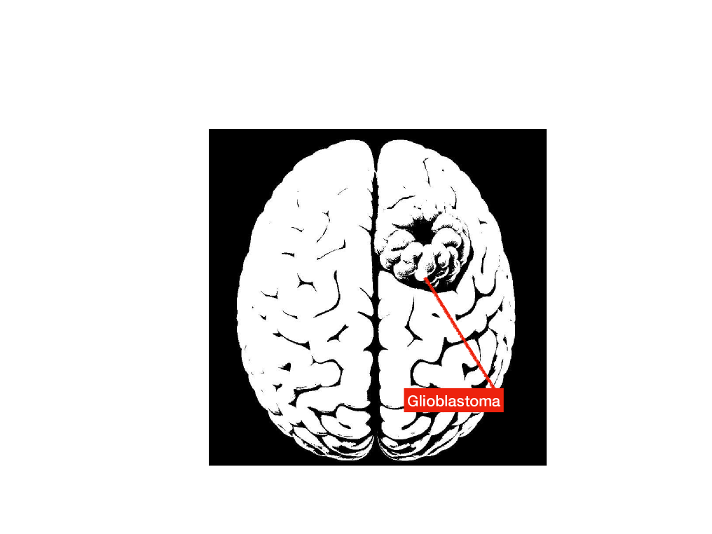
(a)

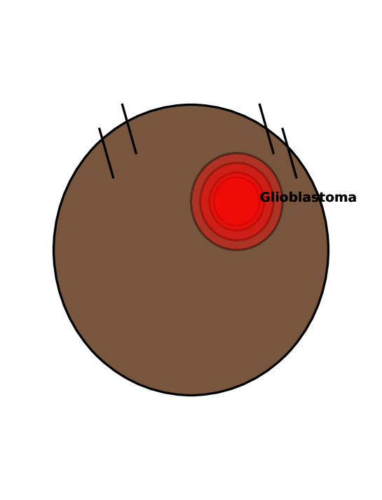
(b)

Figure 1: Illustration of glioblastoma tumor

Accurately predicting tumor progression requires solving a nonlinear PDE that characterizes variations in tumor cell density, including the movement of tumor cells through heterogeneous brain tissues. Proliferation based on available nutrients and carrying capacity. Cell death or treatment effects, such as chemotherapy or immune response. The geometrical illustration of low-grade brain tumors, such as glioblastoma, is shown in Fig. 1.

The tumor growth model can be written as a single equation is the following form:

$$\frac{\partial u}{\partial t}=\nabla\cdot(D\nabla u)+G(u)-K(u),$$ (2.1)

where:

• Rate of change of tumor cell density: $\frac{\partial u}{\partial t}.$

• Diffusion of tumor cells: $\nabla\cdot(D\nabla u).$

• Growth of tumor cells: $G(u)=\rho u\left(1-\frac{u}{K}\right)$, where $\rho$ is a constant.

• Killing rate of tumor cells: $K(u)=\eta u$, where $\eta$ is a constant.

We can write a growth of tumor:

Rate of change of tumor cell density $$=\text{Diffusion of tumor cells}$$

$$\quad+\text{Growth of tumor cells}-\text{Killing rate of tumor cells}.$$ (2.2)

2.1 Models

This work discusses two different models: the Burgesss’ equation and the extended Fisher–Kolmogorov equation. The Burgess equation explain growth of low grades tumors and EFK euation explain brain tumour dynamics. The models are as follows:

2.1.1 Burgess equation

Several studies have analyzed the fundamental model of two-dimensional tumor growth and its governing equation, describing the methodology used for its evaluation. According to these models, tumor cell density evolves based on the combined effects of cell movement and proliferation [38, 20].

$$\partial_{t}\mathcal{U}(t,x) =D\nabla^{2}\mathcal{U}(t,x)+\rho\mathcal{U}(t,x)$$ (2.3)

$$=D\frac{1}{x^{2}}\partial_{x}(x^{2}\partial_{x}\mathcal{U}(t,x))+\rho\mathcal{U}(t,x).$$ (2.4)

The above model can be rewritten as

$$\partial_{t}\mathcal{U}(t,x) =D\frac{1}{x^{2}}\partial_{x}(x^{2}\partial_{x}\mathcal{U}(t,x))+\rho\mathcal{U}(t,x)-k_{t}\mathcal{U}(t,x).$$ (2.5)

The following strategy of [38] and [20]. Let $t=2Dt$, $u(t,x)=x\mathcal{U}(t,x)$ with these equation (2.3) leads to

$$\frac{\partial u(t,x)}{\partial t}=\frac{1}{2}\frac{\partial^{2}u(t,x)}{\partial x^{2}}+\frac{(\rho-k_{t})}{2D}u(t,x).$$ (2.6)

By letting $R(t,x)=\frac{(\rho-k_{t})}{2D}u(t,x)$ equation (2.6) becomes

$$\frac{\partial u(t,x)}{\partial t} =\frac{1}{2}\frac{\partial^{2}u(t,x)}{\partial x^{2}}+R(t,x),\quad \text{on}\quad[0,T]\times\mathbf{D},$$ (2.7)

$$u(0,x) =u_{0}(x),\quad \text{on}\quad\mathbf{D},$$ (2.8)

$$u =\Gamma_{1},\quad u=\Gamma_{2},\quad \text{on}\quad[0,T]\times\partial\mathbf{D}.$$ (2.9)

2.1.2 Extended Fisher–Kolmogorov equation

The EFK equation represents a nonlinear biharmonic equation. It is expressed as [23]

$$u_{t}+\gamma\Delta^{2}u-\Delta u+F(u) =0, \text{on}\quad[0,T]\times\mathbf{D},$$ (2.10)

$$u(0,x) =u_{0}(x), \text{on}\quad\mathbf{D},$$ (2.11)

$$u=\Gamma_{1},\quad\Delta u =\Gamma_{2}, \text{on}\quad[0,T]\times\partial\mathbf{D}.$$ (2.12)

Here, $u_{t}$ represents the time evolution of the tumor cell density, $\gamma\Delta^{2}u$ accounts for higher-order diffusion (biharmonic diffusion), which influences the tumor’s spatial spread but does not represent treatment, $-\Delta u$ corresponds to standard diffusion, describing tumor cell movement, and $F(u)=u^{3}-u$ is a nonlinear reaction term, modeling tumor proliferation.

In this context, $\Gamma_{1}$ and $\Gamma_{2}$ denote given functions, while $t\in[0,T],x\in\mathbf{D}\subset\mathbb{R}^{d}$ and $u\in[0,T]\times\mathbf{D}\rightarrow\mathbb{R}$ represents a confined domain. The parameter $\gamma$ is a strictly positive constant. An essential characteristic of the EFK equation is its energy dissipation law, defined through the energies dissipation law, defined through the energy functional can be written as [41]

$$E(u)=\int\limits_{\mathbf{D}}\left(\frac{\gamma}{2}|\Delta u|^{2}+\frac{1}{2}|\nabla u|^{2}+\frac{1}{4}(1-u^{2})^{2}\right)dx.$$ (2.13)

2.2 The Underlying Abstract PDE

Consider separable Banach spaces $X$ and $Y$ with norms $\|\cdot\|_{X}$ and $\|\cdot\|_{Y}$, respectively. To be precise, define $Y=L^{p}(\mathbbm{D};\mathbb{R}^{m})$ and $X=W^{s,q}(\mathbbm{D};\mathbb{R}^{m})$, where $m\geqslant 1$, $1\leqslant p,q<\infty$, and $s\geqslant 0$, with $\mathbbm{D}\subset{\mathbb{R}}^{\overline{d}}$ for some $\bar{d}\geqslant 1$. $\mathbbm{D}=\mathbf{D}_{T}=[0,T]\times\mathbf{D}\subset\mathbb{R}^{d}$. Let $X^{\ast}\subset X$ and $Y^{\ast}\subset Y$ be closed subspaces equipped with norms $\|\cdot\|_{X^{\ast}}$ and $\|\cdot\|_{Y^{\ast}}$, respectively. The forward problem is well-posed, as all necessary information is available, while the inverse problem is inherently ill-posed due to missing or incomplete information.

2.2.1 Forward problems

The abstract formulation of the governing PDE is

$$\mathcal{D}(u)=\mathbf{f},$$ (2.14)

where $\mathcal{D}$ represents a differential operator mapping $X^{\ast}$ to $Y^{\ast}$, and $\mathbf{f}\in Y^{\ast}$ satisfies the following conditions:

$$\text{(H1)}:\quad\|\mathcal{D}(u)\|_{Y^{\ast}}<\infty,\quad\forall u\in X^{\ast}\text{ with }\|u\|_{X^{\ast}}<\infty.$$ (2.15)

$$\text{(H2)}:\quad\|\mathbf{f}\|_{Y^{\ast}}<\infty.$$

Additionally, assume that for each $\mathbf{f}\in Y^{\ast}$, a unique solution $u\in X^{\ast}$ exists for (2.14), subject to approximate boundary and initial conditions given by

$$\mathcal{B}(u)=u_{b}\quad\text{on }\partial\mathbf{D},\quad u(0,x)=u_{0}\quad\text{on }\mathbf{D}.$$ (2.16)

Here, $\mathcal{B}$ represents a boundary operator, $u_{b}$ is the prescribed boundary data, and $u_{0}(x)$ denotes the initial condition.

2.2.2 Inverse problems

The problem is considered with unknown boundary and initial conditions, rendering the forward problem defined in (2.14) ill-posed. Let the solution $u$ satisfy the given equation within the subdomain $\mathbf{D}^{\prime}_{T}$. The operator $\mathcal{L}$ applied to $u$ in this region is given by a prescribed function $g$ expressed as:

$$\mathcal{L}(u)=g,\quad\forall(t,\bm{x})\in\mathbf{D}^{\prime}_{T}.$$ (2.17)

Here, $\mathbf{D}^{\prime}$ is a subset of $\mathbf{D}$, and the temporal-spatial domain is given by $\mathbf{D}_{T}^{\prime}=[0,T]\times\mathbf{D}^{\prime}\subset[0,T]\times\mathbf{D}$.

2.3 Quadrature Rules

Let $\mathbbm{D}$ represent a domain and $h$ an integrable function defined by $h:\mathbbm{D}\to\mathbb{R}$. Consider the space-time domain $\mathbbm{D}=\mathbf{D}_{T}=[0,T]\times\mathbf{D}\subset\mathbb{R}^{d}$, where $\bar{d}=2d+1\geqslant 1$. The function $h$ is given on $\mathbbm{D}$ as follows:

$$h=\int\limits_{\mathbbm{D}}h(z)\,dz,$$ (2.18)

where $dz$ denotes the $\bar{d}$-dimensional Lebesgue measure. For quadrature, we select points $z_{i}\in\mathbbm{D}$ for $1\leqslant i\leqslant N$, along with corresponding weights $w_{i}$. The quadrature approximation then takes the form:

$$h_{N}=\sum_{i=1}^{N}w_{i}h(z_{i}).$$ (2.19)

Here, $z_{i}$ are the quadrature points. For moderately high-dimensional problems, low-discrepancy sequences such as Sobol and Halton sequences can be employed as quadrature points. For very high-dimensional problems ($d\gg 20$), Monte Carlo quadrature becomes the preferred method for numerical integration [9], where quadrature points are selected randomly and independently.
For a set of weights $w_{i}$ and quadrature points $y_{i}$, we assume that the associated quadrature error adheres to the following bound:

$$\left|\overline{h}-\overline{h}_{N}\right|\leqslant C_{quad}\left(\|h\|_{Z^{\ast}},\bar{d}\right)N^{-\alpha},$$ (2.20)

for some $\alpha>0$.

2.4 Training Points

Physics informed neural networks require four types of training points as described in [33, 34]: interior points $\textit{S}_{\text{int}}$, temporal boundary points $\textit{S}_{\text{tb}}$, spatial boundary points $\textit{S}_{\text{sb}}$, and data points $\textit{S}_{\bm{d}}$. Figs.2 and 3 illustrate the training points used in forward and inverse problems. The training set for forward problems is given by

$$\bm{S}=\textit{S}_{\text{int}}\cup\textit{S}_{\text{sb}}\cup\textit{S}_{\text{tb}}.$$

For the inverse problem, additional training points are required, i.e., data training points $\textit{S}_{\bm{d}}$. The defined training points $\textit{S}_{\text{int/sb/tb}/\bm{d}}$ correspond to quadrature points with weights $w_{j}^{\text{int}/\text{sb}/\text{tb}/\bm{d}}$, determined by an appropriate quadrature rule. In domains $\mathbf{D}$ that are logically rectangular, the training set can be constructed using either Sobol points or randomly selected points. Thus we can define these training points $N$ as following:

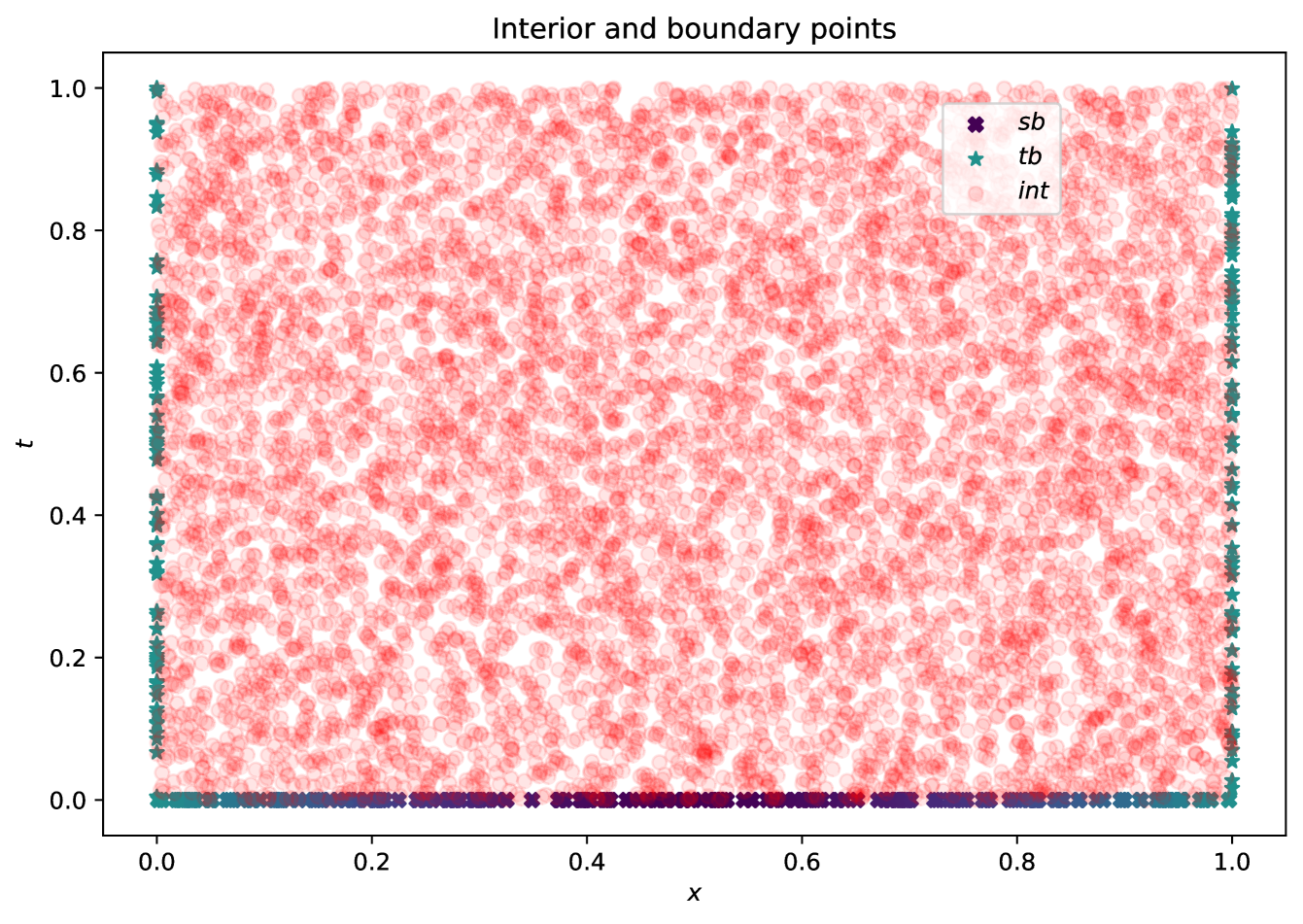
Figure 2: Training points (forward problem): The training set $\bm{S}$ consists of randomly chosen points. Red dots denote interior points, whereas green and blue dots correspond to temporal and spatial boundary points.

2.4.1 Interior training points

The interior training points are denoted by $\textit{S}_{\text{int}}=\left\{z_{j}^{\text{int}}\right\}$ for $1\leqslant j\leqslant N_{\text{int}}$, where $z_{j}^{\text{int}}=\left(t_{j}^{\text{int}},x_{j}^{\text{int}}\right)$. Here, $t_{j}^{\text{int}}\in\left[0,T\right]$, $x_{j}^{\text{int}}\in\mathbf{D}$ for all $j$.

2.4.2 Temporal boundary training points

The temporal boundary points are represented as $\textit{S}_{\text{tb}}=\left\{z_{j}^{\text{tb}}\right\}$, for $1\leqslant j\leqslant N_{\text{tb}}$, with $z_{j}^{\text{tb}}=\left(x_{j}^{\text{tb}}\right)$. Here, $x_{j}^{\text{tb}}\in\mathbf{D}$, $\forall$ $j$.

2.4.3 Spatial boundary training points

The spatial boundary points are denoted as $\textit{S}_{\text{sb}}=\left\{z_{j}^{\text{sb}}\right\}$, for $1\leqslant j\leqslant N_{\text{sb}}$, where $z_{j}^{\text{sb}}=\left(t_{j}^{\text{tb}},x_{j}^{\text{tb}}\right)$. In this case, $t_{j}^{\text{tb}}\in\left[0,T\right]$, $x_{j}^{\text{tb}}\in\partial\mathbf{D}$.

2.4.4 Data training points

The data training set is defined as $\textit{S}_{\bm{d}}=\left\{y_{j}^{\bm{d}}\right\}$ for $1\leqslant j\leqslant N_{\bm{d}}$, where $y_{j}^{\bm{d}}\in\mathbf{D}_{T}^{\prime}$.

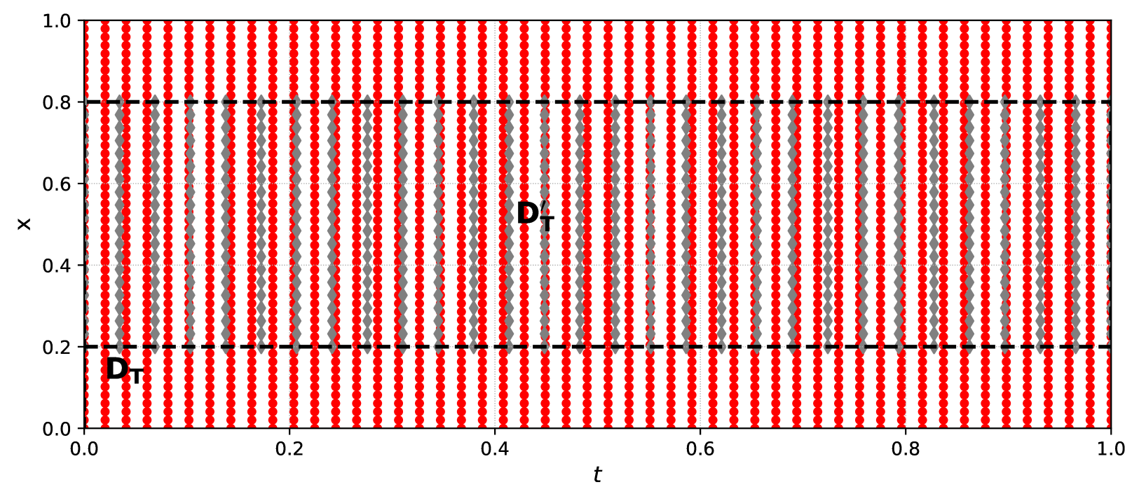
Figure 3: Training points (inverse problem): A visualization of the training set $\bm{S}$ with randomly sampled training points. Red dots denote interior points, while gray dots correspond to Sobol points.

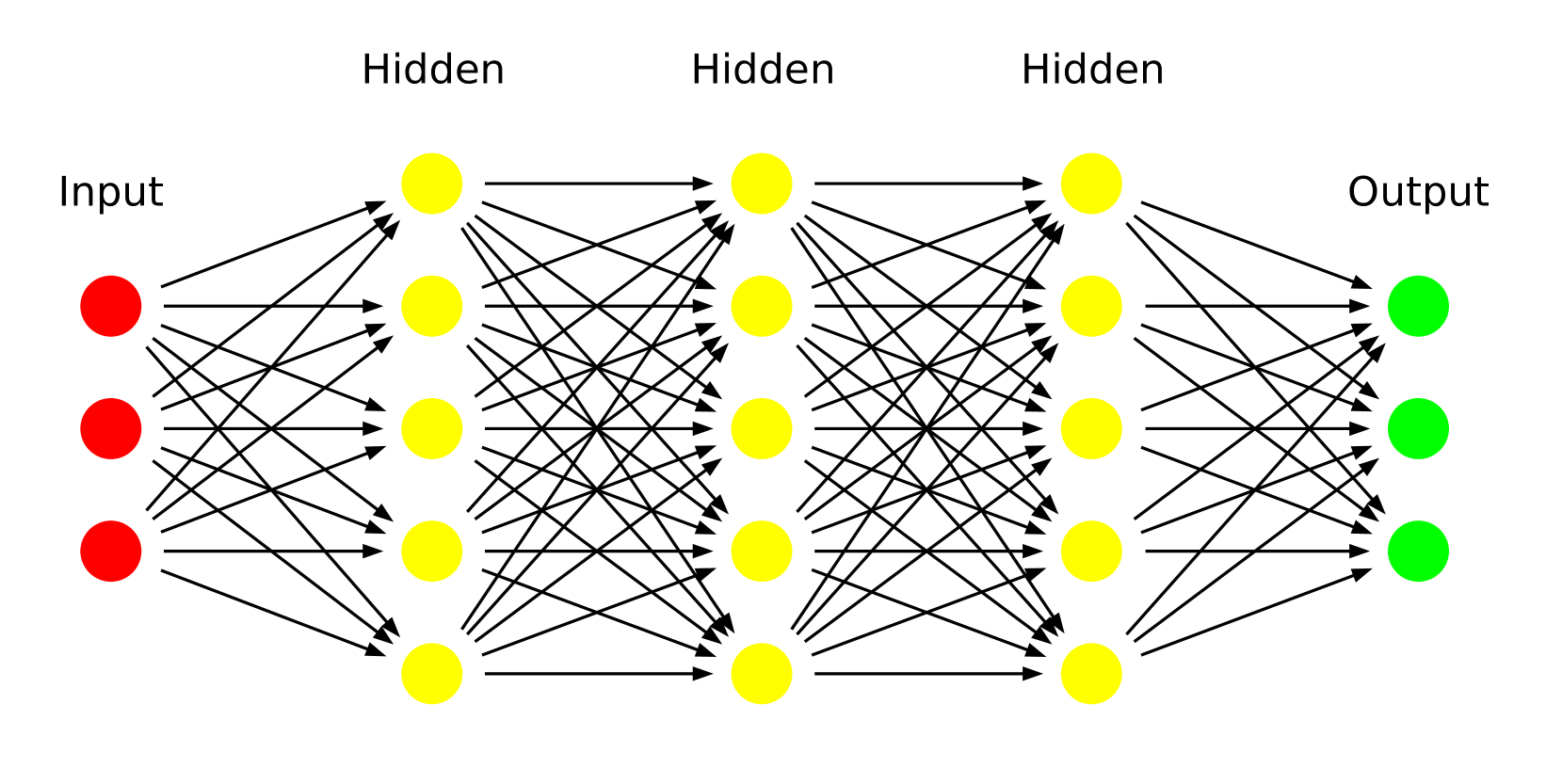
Figure 4: In this diagram, neurons in the input layer are shown in red, those in the hidden layer are represented in yellow, and neurons in the output layer are depicted in green.

2.5 Neural Networks

The PINN operates as a feed-forward neural network, as depicted in Fig. 5. Without an activation function, a neural network functions similarly to a multiple regression model. The activation function introduces non-linearity, enabling the network to learn and perform complex tasks. Examples of activation functions include sigmoid, hyperbolic tangent (tanh), and ReLU [21]. The network receives an input $y=(t,x)\in\mathbbm{D}$, and can be formulated as an affine transformation:

$$u_{\theta}(y)=C_{K}\circ\sigma\circ C_{K-1}\circ\dots\circ\dots\sigma\circ C_{1}(y).$$ (2.21)

Here, $\circ$ denotes function composition, and $\sigma$ represents activation functions. For each layer $k$ where $1\leqslant k\leqslant K$, the transformation is given by:

$$C_{k}z_{k}=W_{k}z_{k}+b_{k},\quad\text{where}\quad W_{k}\in\mathbb{R}^{d_{k+1}\times d_{k}},\,z_{k}\in\mathbb{R}^{d_{k}},\quad\text{and}\quad b_{k}\in\mathbb{R}^{d_{k+1}}.$$ (2.22)

To maintain consistency, we define $d_{1}=\bar{d}=2d+1$, where $d$ is the spatial dimension, and set $d_{K}=1$ for the output layer. Structurally, the network consists of an input layer, an output layer, and $K-1$ hidden layers, subject to the condition $1<K<\mathbb{N}$.

Each hidden layer $k$, comprising $d_{k}$ neurons, processes an input vector $z_{k}\in\mathbb{R}^{d_{k}}$. The transformation begins with the linear mapping $C_{k}$, followed by the application of the activation function $\sigma$. The total number of neurons in the network is given by $2d+2+\sum_{k=2}^{K-1}d_{k}$.

The set of network parameters, including weights and biases, is denoted as $\theta=\left\{W_{k},b_{k}\right\}$. Additionally, the weight parameters alone are represented as $\theta_{w}=\left\{W_{k}\right\}$ for all $1\leqslant k\leqslant K$ [33, 34]. The parameters $\theta$ belong to the space $\theta^{\prime}\subset\mathbb{R}^{P}$, where $P$ represents the total number of parameters:

$$P=\sum_{k=1}^{K-1}\left(d_{k}+1\right)d_{k+1}.$$ (2.23)

2.6 Residuals

This section describes the residuals linked to different training sets, including interior, temporal, spatial and data points used for inverse problems. The primary objective is to minimize these residuals. Optimization will incorporate stochastic gradient descent techniques, such as ADAM for first-order optimization, along with higher-order methods like variants of the BFGS algorithm. The PINN $u_{\theta}$ depends on tuning parameters $\theta\in\theta^{\prime}$, which correspond to the network’s weights and biases. In a standard deep learning framework, training involves adjusting these parameters to ensure that the neural network approximation $u_{\theta}$ closely matches the exact solution $u$. The interior residual is defined as:

$$\mathfrak{R}_{\text{int},\theta}=\mathfrak{R}_{\text{int},\theta}(t,x),\quad\forall(t,x)\in[0,T]\times\mathbf{D}.$$ (2.24)

It can be expressed in terms of the differential operator as follows:

$$\mathfrak{R}_{\text{int},\theta}=\mathcal{D}(u_{\theta})-\mathbf{f}.$$ (2.25)

The residual formulation of our models, given in Eq. (2.6) and Eq. (2.10), can be written as:

$$\mathfrak{R}_{\text{int},\theta} =\partial_{t}u_{\theta}-0.5\partial_{xx}u_{\theta}-R(u_{\theta})$$ (2.26)

$$\mathfrak{R}_{\text{int},\theta} =\partial_{t}u_{\theta}+\gamma\Delta^{2}u_{\theta}-\Delta u_{\theta}+F(u_{\theta}).$$

Residuals corresponding to initial, boundary, and data points are formulated as:

$$\mathfrak{R}_{\text{tb}} =\mathfrak{R}_{\text{tb},\theta}=u_{\theta}-u_{0},\quad\forall x\in\mathbf{D},$$ (2.27)

$$\mathfrak{R}_{\text{sb}} =\mathfrak{R}_{\text{sb},\theta}=u_{\theta}-u_{b},\quad\forall(t,x)\in\partial{\mathbf{D}}.$$

Additionally, the residual for data points is given by:

$$\mathfrak{R}_{{\bm{d}}}=\mathcal{L}(u_{\theta})-g,\quad\forall(t,x)\in\mathbf{D}^{\prime}_{T}.$$ (2.28)

The goal is to determine the optimal tuning parameters $\theta\in\theta^{\prime}$ that minimize the residual in the forward problem:

$$\theta^{\ast}\in\theta^{\prime}:\theta^{\ast}=\arg\min_{\theta\in\theta^{\prime}}\left(\|\mathfrak{R}_{\text{int},\theta}\|^{2}_{L^{2}(\mathbf{D}_{T})}+\|\mathfrak{R}_{\text{sb},\theta}\|^{2}_{L^{2}(\mathbf{[0,T]\times\partial D})}+\|\mathfrak{R}_{\text{tb},\theta}\|^{2}_{L^{2}(\mathbf{D})}\right).$$ (2.29)

For the inverse problem, an additional term corresponding to the data residual $\mathrm{R}_{\bm{d}}$ is introduced in Eq. (2.29), leading to the following minimization problem:

$$\theta^{\ast}\in\theta^{\prime}:\theta^{\ast}=\arg\min_{\theta\in\theta^{\prime}}\left(\|\mathfrak{R}_{\text{int},\theta}\|^{2}_{L^{2}(\mathbf{D}_{T})}+\|\mathfrak{R}_{\text{sb},\theta}\|^{2}_{L^{2}(\mathbf{[0,T]\times\partial D})}+\|\mathfrak{R}_{\bm{d},\theta}\|^{2}_{L^{2}(\mathbf{D}^{\prime}_{T})}+\|\mathfrak{R}_{\text{tb},\theta}\|^{2}_{L^{2}(\mathbf{D})}\right).$$ (2.30)

Since the integrals in Eqs. (2.29) and (2.30) involve the $L^{2}$ norm, an exact computation is not feasible. Instead, numerical quadrature methods are employed for approximation.

2.7 Loss Functions and Optimization

The integrals (2.25) is approximated using the following loss functions for forward problems:

$$\mathscr{L}_{1}(\theta)=\sum\limits_{j=1}^{N_{sb}}w_{j}^{sb}|\mathfrak{R}_{\text{sb},\theta}(z_{j}^{sb})|^{2}+\sum\limits_{j=1}^{N_{tb}}w_{j}^{tb}|\mathfrak{R}_{\text{tb},\theta}(z_{j}^{tb})|^{2}+\lambda\sum\limits_{j=1}^{N_{int}}w_{j}^{int}|\mathfrak{R}_{\text{int},\theta}(z_{j}^{int})|^{2},$$ (2.31)

The integrals (2.27) is approximated using the following loss functions for inverse problems:

$$\mathscr{L}_{2}(\theta)=\sum\limits_{j=1}^{N_{d}}w_{j}^{d}|\mathfrak{R}_{\bm{d},\theta}(z_{j}^{d})|^{2}+\sum\limits_{j=1}^{N_{sb}}w_{j}^{sb}|\mathfrak{R}_{\text{sb},\theta}(z_{j}^{sb})|^{2}+\sum\limits_{j=1}^{N_{tb}}w_{j}^{tb}|\mathfrak{R}_{\text{tb},\theta}(z_{j}^{tb})|^{2}+\lambda\sum\limits_{j=1}^{N_{int}}w_{j}^{int}|\mathfrak{R}_{\text{int},\theta}(z_{j}^{int})|^{2}.$$ (2.32)

The loss function minimization is regularized as follows:

$$\theta^{\ast}=\arg\min_{\theta\in\theta^{\prime}}(\mathscr{L}_{i}(\theta)+\lambda_{reg}\mathscr{L}_{reg}(\theta)),$$ (2.33)

where $i=1,2$. In deep learning, regularization helps prevent over-fitting. A common form of regularization is $\mathscr{L}_{\text{reg}}(\theta)=\|\theta\|_{q}^{q}$, where $q=1$ (for $L^{1}$ regularization) or $q=2$ (for $L^{2}$ regularization). The regularization parameter $\lambda_{\text{reg}}$ balances the trade-off between the loss function $\mathscr{L}$ and the regularization term, where $0\leqslant\lambda_{\text{reg}}\ll 1$. Stochastic gradient descent algorithms such as ADAM will be used for optimization, as they are widely adopted for first-order methods. Additionally, second-order optimization strategies, including different versions of the BFGS algorithm, may be employed. The objective is to determine the optimal neural network solution $u^{\ast}=u_{\theta^{\ast}}$ using the training dataset. The process begins with an initial parameter set $\bar{\theta}\in\theta^{\prime}$, and the corresponding network output $u_{\bar{\theta}}$, residuals, loss function, and gradients are computed iteratively. Ultimately, the optimal solution, denoted as $u^{\ast}=u_{\theta^{\ast}}$, is obtained through PINN. The local minimum in Eq. (2.33) is approximated as $\theta^{\ast}$, yielding the deep neural network solution $u^{\ast}=u_{\theta^{\ast}}$, which serves as an approximation to $u$ in low grades tumors models.

The hyper-parameters used in numerical experiments are summarized in Table 1. The PINN framework for solving the low grades tumors models follows the methodologies outlined in [33, 34, 4, 35]. The illustration in Fig. 5 represents the PINN framework. Below, Algorithm 2.1 is presented for forward problems, while Algorithm 2.2 addresses inverse problems:

Table 1: The configurations of hyper-parameters and the frequency of retraining utilized in ensemble training for PINN.

Experiments	$K-1$	$\bar{d}$	$\lambda$	$\lambda_{\text{reg}}$	$n_{\theta}$
3.1.1	4	20	0.1, 1, 10	0	4
3.1.2	4	20	0.1, 1, 10	0	10
3.1.3	4	20	0.1, 1, 10	0	4
3.1.4	4	20	0.1, 1, 10	0	12
3.1.5	4	32	0.1, 1, 10	0	10
3.2.1	4	16	0.1, 1, 10	0	10
3.2.2	4	20	0.1, 1, 10	0	10
3.2.3	4	24, 36, 42	0.1, 1, 10	0	10,10,4

Algorithm 2.1.

The PINN framework is employed for estimating low-grade tumors in forward problems

• Define the computational domain, problem data, and coefficients for the low grade tumor models. Specify quadrature points and weights for numerical integration. Choose a gradient-based optimization method for training the neural network.

• Develop a PINN approximation $u^{\ast}=u_{\theta^{\ast}}$ for solving the model.

• Select the training points following the methodology described in Section 2.4.

• Initialize the network with parameters $\bar{\theta}\in\theta^{\prime}$ and compute the following: neural network output $u_{\bar{\theta}}$ Eq. (2.21), PDE residual Eq. (2.25), boundary residuals Eq. (2.27), loss function Eq. (2.31), Eq. (2.33), and gradients required for optimization.

• Apply the optimization algorithm iteratively until an approximate local minimum $\theta^{\ast}$ of Eq. (2.33) is obtained. The trained network $u^{\ast}=u_{\theta^{\ast}}$ serves as the PINN solution for the tumor growth models.

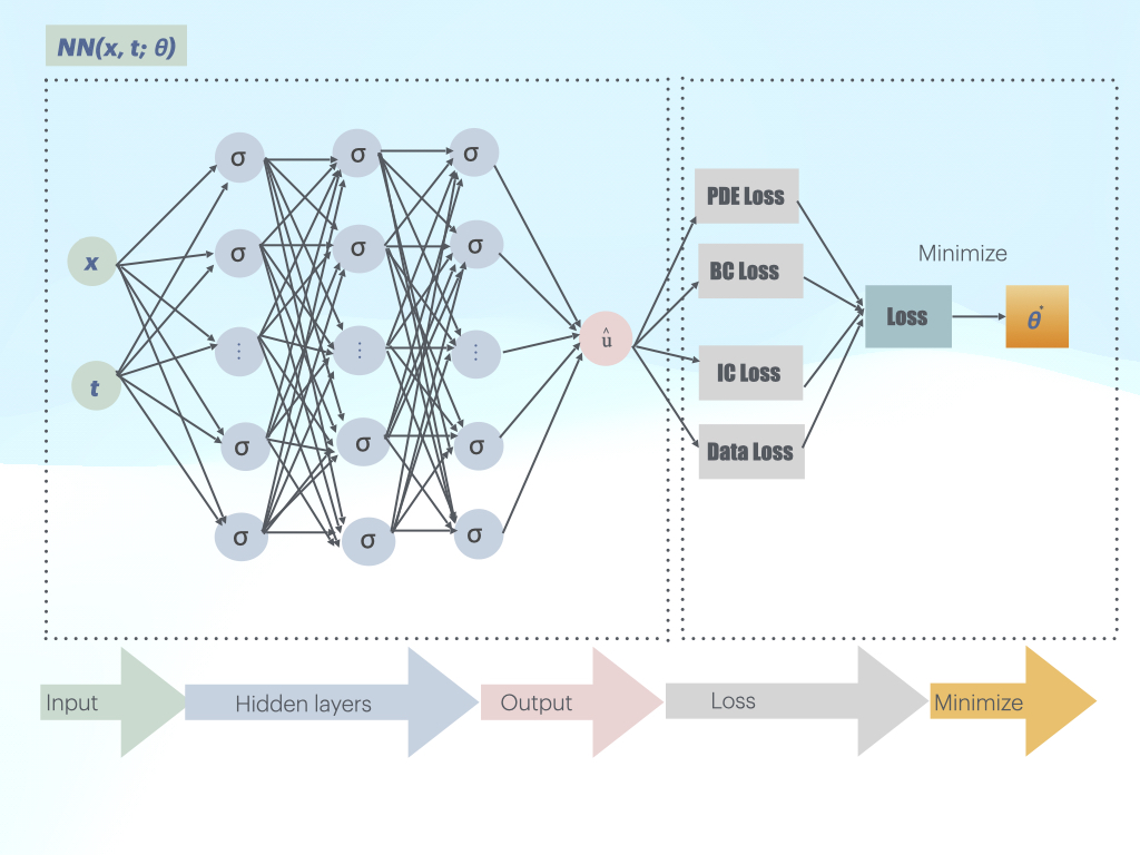
Figure 5: Schematic representation of the PINN framework.

Algorithm 2.2.

The PINN framework is employed for estimating low-grade tumors in s inverse problems

• Define the computational domain, problem data, and coefficients for the low-grade tumor model. Specify quadrature points and weights for numerical integration. Choose a suitable non-convex gradient-based optimization method.

• Construct a PINN approximation $u^{\ast}=u_{\theta^{\ast}}$ to estimate the solution $u$ of low grade tumor models for inverse problems.

• Select training points according to the methodology outlined in Section 2.4.

• Initialize the neural network with parameters $\bar{\theta}\in\theta^{\prime}$ and compute the following components: neural network output $u_{\bar{\theta}}$ Eq. (2.21), PDE residual Eq. (2.25), data residuals Eq. (2.28), loss function Eq. (2.32), Eq. (2.33), and gradients for optimization.

• Apply the optimization algorithm iteratively until an approximate local minimum $\theta^{\ast}$ of Eq. (2.33) is reached. The trained network $u^{\ast}=u_{\theta^{\ast}}$ serves as the PINN solution for the low-grade tumor model.

2.8 Estimation on Generalization Error

Let the spatial domain be $\mathbf{D}=[0,1]^{d}$, where $d$ denotes the spatial dimension. This section focuses on obtaining an accurate estimation of the generalization error, also referred to as the total error, for the trained neural network $u^{\ast}=u_{\theta^{\ast}}$. This result arises from the application of the PINN algorithms 2.1 and 2.2. The error can be expressed as follows:

$$\bm{\mathcal{E}}_{G}:=\left(\int\limits_{0}^{T}\int\limits_{0}^{1}|u(t,x)-u^{\ast}(t,x)|^{2}dxdt\right)^{\frac{1}{2}}.$$ (2.34)

This approach is outlined in [33], [4], [34] and [35]. This section provides an estimation of the generalization error, as defined in equation (2.34), based on the training error. For the abstract PDE equation (2.14), the generalization error is analyzed by expressing it in terms of the training error, which is defined as follows:

$$(\bm{\mathcal{E}}_{T}^{int})^{2} =\sum\limits_{n=1}^{N_{int}}w^{int}_{n}|\mathfrak{R}_{int,\theta^{\ast}}|^{2},\quad(\bm{\mathcal{E}}_{T}^{sb})^{2}=\sum\limits_{n=1}^{N_{sb}}w^{sb}_{n}|\mathfrak{R}_{sb,\theta^{\ast}}|^{2},$$

$$(\bm{\mathcal{E}}_{T}^{tb})^{2} =\sum\limits_{n=1}^{N_{tb}}w^{tb}_{n}|\mathfrak{R}_{tb,\theta^{\ast}}|^{2},\quad(\bm{\mathcal{E}}_{T}^{d})^{2}=\sum\limits_{n=1}^{N_{\bm{d}}}w^{\bm{d}}_{n}|\mathfrak{R}_{\bm{d},\theta^{\ast}}|^{2}.$$ (2.35)

For the EFK equation, we modify $\bm{\mathcal{E}}_{T}^{sb}$ as in [4]:

$$(\bm{\mathcal{E}}_{T}^{sb})^{2}=\sum\limits_{n=1}^{N_{sb}}\sum\limits_{i=1}^{4}w^{sb}_{n}|\mathfrak{R}_{sbi,\theta^{\ast}}|^{2}.$$ (2.36)

The training error can be directly computed a posteriori using the loss function equation (2.33). Additionally, the following assumptions on the quadrature error are required, similar to equations (2.33) and (2.32). For any function $h\in C^{k}(\mathbf{D})$, the quadrature rule, defined using quadrature weights $w^{tb}_{n}$ at points $x_{n}\in\mathcal{S}_{tb}$ for $1\leqslant n\leqslant N_{tb}$, satisfies the bound

$$\left|\int\limits_{\mathbf{D}}h(x)dx-\sum\limits_{n=1}^{N_{tb}}w^{tb}_{n}h(x_{n})\right|\leqslant C^{tb}_{quad}(\|h\|_{C^{k}})N_{tb}^{-\alpha_{tb}}.$$ (2.37)

For any function $g\in C^{k}(\partial\mathbf{D}\times[0,T])$, the quadrature rule corresponding to quadrature weights $w^{sb}_{n}$ at points $(x_{n},t_{n})\in\mathcal{S}_{sb}$, with $1\leqslant n\leqslant N_{sb}$, satisfies

$$\left|\int\limits_{0}^{T}\int\limits_{\partial\mathbf{D}}h(x,t)ds(x)dt-\sum\limits_{n=1}^{N_{sb}}w^{sb}_{n}h(x_{n},t_{n})\right|\leqslant C^{sb}_{quad}(\|h\|_{C^{k}})N_{sb}^{-\alpha_{sb}}.$$ (2.38)

Finally, for any function $h\in C^{\ell}(\mathbf{D}\times[0,T])$, the quadrature rule corresponding to quadrature weights $w^{int}_{n}$ at points $(x_{n},t_{n})\in\mathcal{S}_{int}$, with $1\leqslant n\leqslant N_{int}$, satisfies

$$\left|\int\limits_{0}^{T}\int\limits_{\mathbf{D}}h(x,t)dxdt-\sum\limits_{n=1}^{N_{int}}w^{int}_{n}h(x_{n},t_{n})\right|\leqslant C^{int}_{quad}(\|h\|_{C^{\ell}})N_{int}^{-\alpha_{int}}.$$ (2.39)

In the above, $\alpha_{int},\alpha_{sb},\alpha_{tb}>0$ and in principle, different-order quadrature rules can be used. The generalization error for the Burgess equation and the EFK equation, obtained using Algorithm 2.1, is given in the following form:

$$\bm{\mathcal{E}}_{G}\leqslant C_{1}\left(\bm{\mathcal{E}}_{T}^{tb}+\bm{\mathcal{E}}_{T}^{int}+C_{2}(\bm{\mathcal{E}}_{T}^{sb})^{\frac{1}{2}}+(C_{quad}^{tb})^{\frac{1}{2}}N_{tb}^{-\frac{\alpha_{tb}}{2}}+(C_{quad}^{int})^{\frac{1}{2}}N_{int}^{-\frac{\alpha_{int}}{2}}+C_{2}(C_{quad}^{sb})^{\frac{1}{4}}N_{sb}^{-\frac{\alpha_{sb}}{4}}\right),$$ (2.40)

where the constants $C_{1}$ and $C_{2}$ are shown in Appendix E.1 and Appendix E.2.

2.9 Stability and Convergence of Multilayer Neural Network

This section presents the stability and convergence analysis of the neural network for both models. For convenience, let $u_{\theta}=U$.

2.9.1 Stability of multilayer neural network

Here, $L^{\infty}$ bounds are derived for both models.

Theorem 2.3.

Let $U$ be a neural network solution to the equation

$$\frac{\partial U}{\partial t}=\frac{1}{2}\frac{\partial^{2}U}{\partial x^{2}}+R(U),$$ (2.41)

where the reaction term $R(U)$ satisfies the Lipchitz condition Appendix E.6 along with one of the following conditions:

• (i) Linear growth condition: If there exists a constant $C>0$ such that

  $$|R(U)|\leqslant C(1+|U|),$$ (2.42)

  then $U$ is uniformly bounded in $L^{2}(\mathbf{D})$, i.e., there exists a constant $M>0$ such that

  $$\sup_{t\in[0,T]}\|U(t)\|_{L^{2}(\mathbf{D})}\leqslant M.$$ (2.43)

• (ii) Exponential decay condition

  $$|R(U)|\leqslant Ce^{-\alpha U},$$ (2.44)

  for some constants $C,\alpha>0$. Then $U$ is uniformly bounded in $L^{\infty}(\mathbf{D})$ and satisfies the estimate:

  $$\sup_{t\in[0,T]}\|U(t)\|_{L^{\infty}(\mathbf{D})}\leqslant C^{\prime}e^{-\beta t}\|U_{0}\|_{L^{2}(\mathbf{D})},$$ (2.45)

  for some constant $C^{\prime}>0$, decay rate $\beta>0$ and initial condition $U_{0}$.

Proof.

Multiplying the equation (2.41) by $U$ and integrating over $\mathbf{D}$:

$$\int_{\mathbf{D}}U\frac{\partial U}{\partial t}\,dx=\frac{1}{2}\int_{\mathbf{D}}U\frac{\partial^{2}U}{\partial x^{2}}\,dx+\int_{\mathbf{D}}UR(U)\,dx.$$ (2.46)

Using integration by part and the Dirichlet boundary condition $U=0$ on $\partial\mathbf{D}$,

$$\int_{\mathbf{D}}U\frac{\partial^{2}U}{\partial x^{2}}\,dx=-\int_{\mathbf{D}}\left(\frac{\partial U}{\partial x}\right)^{2}\,dx\leqslant 0.$$ (2.47)

Thus,

$$\int_{\mathbf{D}}U\frac{\partial U}{\partial t}\,dx\leqslant\int_{\mathbf{D}}UR(U)\,dx.$$ (2.48)

Applying the Linear Growth Condition,

$$\int_{\mathbf{D}}UR(U)\,dx\leqslant C\int_{\mathbf{D}}(1+|U|^{2})\,dx.$$ (2.49)

Using Gronwall’s inequality,

$$\sup_{t\in[0,T]}\|U(t)\|_{L^{2}(\mathbf{D})}\leqslant M.$$ (2.50)

Multiply equation (2.41) by $|U|^{p-2}U$ and integrate over $\mathbf{D}$:

$$\int_{\mathbf{D}}|U|^{p-2}U\frac{\partial U}{\partial t}\,dx=\frac{1}{2}\int_{\mathbf{D}}|U|^{p-2}U\frac{\partial^{2}U}{\partial x^{2}}\,dx+\int_{\mathbf{D}}|U|^{p-2}UR(U)\,dx.$$ (2.51)

Using integration by parts and the Dirichlet boundary condition:

$$\int_{\mathbf{D}}|U|^{p-2}U\frac{\partial^{2}U}{\partial x^{2}}\,dx=-(p-1)\int_{\mathbf{D}}|U|^{p-2}\left(\frac{\partial U}{\partial x}\right)^{2}\,dx\leqslant 0.$$ (2.52)

Thus,

$$\int_{\mathbf{D}}|U|^{p-2}U\frac{\partial U}{\partial t}\,dx\leqslant\int_{\mathbf{D}}|U|^{p-2}UR(U)\,dx.$$ (2.53)

Applying the exponential decay condition:

$$\int_{\mathbf{D}}|U|^{p-2}UR(U)\,dx\leqslant C\int_{\mathbf{D}}|U|^{p-2}Ue^{-\alpha U}\,dx.$$ (2.54)

For large $|U|$, the term

$$|U|^{p-1}e^{-\alpha U}\leqslant Ce^{-\alpha U/2}.$$ (2.55)

Since $e^{-\alpha U/2}$ decays exponentially and dominates any polynomial growth, the integral remains bounded. Using Moser’s iteration,

$$\sup_{t\in[0,T]}\|U(t)\|_{L^{\infty}(\mathbf{D})}\leqslant C^{\prime}e^{-\beta t}\|U_{0}\|_{L^{2}(\mathbf{D})}.$$ (2.56)

This proves that $U$ remains strictly bounded in $L^{\infty}$ with exponential decay. ∎

Theorem 2.4.

Suppose that the EFK equation satisfies the Lipschitz condition of Lemma Appendix E.7, and the neural network solution $U$ preserves an energy dissipation law. Moreover, let $U_{0}\in H^{2}_{0}(\mathbf{D})$, so that the energy dissipation property holds:

$$E(U)\leqslant E(U_{0}).$$ (2.57)

Then, the solution $U$ is bounded in the $L^{\infty}$-norm.

Proof.

The energy function in neural network $U$ terms is defined as from eq (2.13):

$$E(U)=\int_{\mathbf{D}}\left(\frac{\gamma}{2}|\Delta U|^{2}+\frac{1}{2}|\nabla U|^{2}+\frac{1}{4}(1-U^{2})^{2}\right)dx.$$ (2.58)

Differentiating $E(U)$ with respect to time:

$$\frac{dE}{dt}=\int_{\mathbf{D}}\left(\frac{\gamma}{2}\frac{d}{dt}|\Delta U|^{2}+\frac{1}{2}\frac{d}{dt}|\nabla U|^{2}+\frac{1}{4}\frac{d}{dt}(1-U^{2})^{2}\right)dx.$$ (2.59)

First term: $\frac{d}{dt}|\Delta U|^{2}$
Since $|\Delta U|^{2}=(\Delta U)^{2}$, differentiation gives:

$$\frac{d}{dt}|\Delta U|^{2}=2\Delta U\cdot\Delta U_{t}.$$ (2.60)

Thus,

$$\frac{d}{dt}\frac{\gamma}{2}|\Delta U|^{2}=\gamma\Delta U\cdot\Delta U_{t}.$$ (2.61)

Second Term: $\frac{d}{dt}|\nabla U|^{2}$ Expanding $|\nabla U|^{2}$ as $\sum_{i=1}^{d}(\partial_{x_{i}}U)^{2}$, differentiation gives:

$$\frac{d}{dt}|\nabla U|^{2}=2\nabla U\cdot\nabla U_{t}.$$ (2.62)

Thus,

$$\frac{d}{dt}\frac{1}{2}|\nabla U|^{2}=\nabla U\cdot\nabla U_{t}.$$ (2.63)

Applying integration by parts:

$$\int_{\mathbf{D}}\nabla U\cdot\nabla U_{t}dx=-\int_{\mathbf{D}}(\Delta U)U_{t}dx.$$ (2.64)

Third Term: $\frac{d}{dt}(1-U^{2})^{2}$ Using the chain rule:

$$\frac{d}{dt}(1-U^{2})^{2}=-4U(1-U^{2})U_{t}.$$ (2.65)

Thus,

$$\frac{d}{dt}\frac{1}{4}(1-U^{2})=-U(1-U^{2})U_{t}.$$ (2.66)

Substituting into $\frac{dE}{dt}$,

$$\frac{dE}{dt}=\int_{\mathbf{D}}\left[\gamma\Delta U\cdot\Delta U_{t}-(\Delta U)U_{t}-U(1-U^{2})U_{t}\right]dx.$$ (2.67)

Rewriting:

$$\frac{dE}{dt}=\int_{\mathbf{D}}U_{t}\left(\gamma\Delta^{2}U-\Delta U-U(1-U^{2})\right)dx.$$ (2.68)

If $U$ satisfies the evolution equation (2.10):

$$U_{t}=-(\gamma\Delta^{2}U-\Delta U-U(1-U^{2})),$$ (2.69)

substituting into $\frac{dE}{dt}$ gives:

$$\frac{dE}{dt}=\int_{\mathbf{D}}-(\gamma\Delta^{2}U-\Delta U-U(1-U^{2}))^{2}dx.$$ (2.70)

Since the integrand is non-positive,

$$\frac{dE}{dt}\leqslant 0.$$ (2.71)

Thus, $E(U)$ is non-increasing, ensuring energy dissipation and stability of the system.

$$E(U)\leqslant E(U_{0}).$$ (2.72)

Using Poincaré’s inequality in the energy dissipation property,

$$\|U\|_{L^{2}}\leqslant C\frac{1}{\gamma}\|U_{0}\|_{L^{2}}.$$ (2.73)

An application of the Sobolev embedding theorem then gives

$$\|U\|_{L^{\infty}}\leqslant C\frac{1}{\gamma}\|U_{0}\|_{L^{2}}.$$ (2.74)

Thus, $U$ is uniformly bounded in $L^{\infty}$, completing the proof. ∎

2.9.2 Convergence of multilayer neural network

This section establishes $L^{2}$ bounds and analyzes the convergence of the multilayer neural network $U^{n}$ for both models. From 2.2.1

$$\mathcal{D}(U^{n})=\mathbf{f}.$$ (2.75)

Additionally, assume that for each $\mathbf{f}\in Y^{\ast}$, a unique solution $u\in X^{\ast}$ exists for (2.14), subject to approximate boundary and initial conditions given by

$$\mathcal{B}(U^{n})=U_{b}^{n}\quad\text{on }\partial\mathbf{D},\quad U^{n}(0,x)=U^{n}_{0}\quad\text{on }\mathbf{D}.$$ (2.76)

Here, $\mathcal{B}$ represents a boundary operator, $U_{b}^{n}$ is the prescribed boundary data, and $U^{n}_{0}$ denotes the initial condition.

Theorem 2.5.

Let $U^{n}_{0}\in H^{1}_{0}(\mathbf{D})$ be the initial neural network approximation of the Burgess equation. Under the assumptions of lemma Appendix E.5, there exists a unique solution $u\in H^{1}(\mathbf{D})\cap H^{2}(\mathbf{D})$ to the Burgess equation. Assume that the Burgess equation satisfies the Lipschitz condition given in Appendix E.6, and that the sequence $\{U^{n}\}$ is uniformly bounded in $L^{2}([0,T];H^{1}(\mathbf{D}))$. Then, the approximate solution $U^{n}$ satisfies the following properties:

1. Strong convergence in $L^{2}$: $U^{n}\to u$ strongly in $L^{2}(\mathbf{D})$.

2. Uniform convergence: $U^{n}$ converges uniformly to $u$ in $\mathbf{D}$.

Suppose $U^{n}$ satisfies the PDE in a bounded domain $\mathbf{D}$ with homogeneous Dirichlet boundary conditions:

$$\frac{\partial U^{n}}{\partial t}=\frac{1}{2}\Delta U^{n}+R(U^{n}),$$ (2.77)

where the reaction term $R(U^{n})$ satisfies one of the following conditions:

1. Linear Growth Condition:

   $$|R(U^{n})|\leqslant C(1+|U^{n}|),\quad\text{for some constant }C>0.$$ (2.78)

   Under this condition, there exists a constant $M>0$ such that:

   $$\sup_{t\in[0,T]}\|U^{n}(t)\|_{L^{2}(\mathbf{D})}\leqslant M.$$ (2.79)

2. Exponential decay condition:

   $$|R(U^{n})|\leqslant Ce^{-\lambda|U^{n}|},\quad\text{for some constants }C>0,\lambda>0.$$ (2.80)

   In this case, $U^{n}$ exhibits moderate decay properties, ensuring:

   • Boundedness in $L^{2}(\mathbf{D})$,

Under the above assumptions, the sequences $\{U^{n}\}$ and $\{\Delta U^{n}\}$ remain uniformly bounded in $L^{2}(\mathbf{D})$ and $H^{2}(\mathbf{D})$, respectively.

Proof.

To prove that the sequence $\{U^{n}\}$ is uniformly bounded in $L^{2}(\mathbf{D})$, we use energy estimates. The sequence $U^{n}$ satisfies the PDE:

$$\frac{\partial U^{n}}{\partial t}=\frac{1}{2}\Delta U^{n}+R(U^{n}),$$ (2.81)

in a bounded domain $\mathbf{D}$ with homogeneous Dirichlet boundary conditions. Taking the $L^{2}(\mathbf{D})$-inner product with $U^{n}$, we obtain:

$$\left\langle\frac{\partial U^{n}}{\partial t},U^{n}\right\rangle=\left\langle\frac{1}{2}\Delta U^{n},U^{n}\right\rangle+\left\langle R(U^{n}),U^{n}\right\rangle.$$ (2.82)

Using integration by parts and the boundary condition $U^{n}=0$ on $\partial\mathbf{D}$, we get:

$$\left\langle\Delta U^{n},U^{n}\right\rangle=-\|\nabla U^{n}\|^{2}_{L^{2}(\mathbf{D})}.$$ (2.83)

Thus, the equation simplifies to:

$$\frac{d}{dt}\|U^{n}\|^{2}_{L^{2}(\mathbf{D})}=-\|\nabla U^{n}\|^{2}_{L^{2}(\mathbf{D})}+2\left\langle R(U^{n}),U^{n}\right\rangle.$$ (2.84)

Bounding the Reaction Term We consider the two different reaction term conditions. Linear Growth Condition

$$|R(U^{n})|\leqslant C(1+|U^{n}|).$$ (2.85)

Applying Hölder’s inequality:

$$\left\langle R(U^{n}),U^{n}\right\rangle\leqslant C\int_{\mathbf{D}}(1+|U^{n}|)|U^{n}|dx.$$ (2.86)

Thus,

$$\left\langle R(U^{n}),U^{n}\right\rangle\leqslant C\left(\|U^{n}\|^{2}_{L^{2}(\mathbf{D})}+\|U^{n}\|_{L^{2}(\mathbf{D})}\right).$$ (2.87)

Using Young’s inequality, for some constant $C_{1}$:

$$\|U^{n}\|_{L^{2}(\mathbf{D})}\leqslant\frac{1}{2}\|U^{n}\|^{2}_{L^{2}(\mathbf{D})}+C_{1}.$$ (2.88)

Thus, we obtain:

$$\left\langle R(U^{n}),U^{n}\right\rangle\leqslant C_{2}\|U^{n}\|^{2}_{L^{2}(\mathbf{D})}+C_{3}.$$ (2.89)

Using this in the energy estimate:

$$\frac{d}{dt}\|U^{n}\|^{2}_{L^{2}(\mathbf{D})}\leqslant C_{2}\|U^{n}\|^{2}_{L^{2}(\mathbf{D})}+C_{3}.$$ (2.90)

Applying Gronwall’s inequality, we conclude:

$$\|U^{n}(t)\|^{2}_{L^{2}(\mathbf{D})}\leqslant M,$$ (2.91)

Exponential Decay Condition

$$|R(U^{n})|\leqslant Ce^{-\zeta|U^{n}|}.$$ (2.92)

Since $e^{-\zeta|U^{n}|}$ decays exponentially, the reaction term does not cause uncontrolled growth. More formally, since:

$$|U^{n}R(U^{n})|\leqslant C|U^{n}|e^{-\zeta|U^{n}|}\leqslant C,$$ (2.93)

It follows that:

$$\left\langle R(U^{n}),U^{n}\right\rangle\leqslant C_{4}.$$ (2.94)

Thus, the energy estimate simplifies to:

$$\frac{d}{dt}\|U^{n}\|^{2}_{L^{2}(\mathbf{D})}\leqslant C_{4}.$$ (2.95)

Integrating over $t$, we obtain:

$$\|U^{n}(t)\|^{2}_{L^{2}(\mathbf{D})}\leqslant\|U^{n}(0)\|^{2}_{L^{2}(\mathbf{D})}+C_{4}T.$$ (2.96)

This implies uniform boundedness. In both cases, we have shown that there exists a constant $M>0$ such that:

$$\sup_{t\in[0,T]}\|U^{n}(t)\|_{L^{2}(\mathbf{D})}\leqslant M.$$ (2.97)

To prove that $\{\Delta U^{n}\}$ is uniformly bounded in $L^{2}(\mathbf{D})$, we derive an energy estimate. Taking the Laplacian of the PDE The given equation is:

$$\frac{\partial U^{n}}{\partial t}=\frac{1}{2}\Delta U^{n}+R(U^{n}).$$ (2.98)

Applying the Laplacian $\Delta$ on both sides,

$$\frac{\partial}{\partial t}\Delta U^{n}=\frac{1}{2}\Delta^{2}U^{n}+\Delta R(U^{n}).$$ (2.99)

Testing with $\Delta U^{n}$ Taking the $L^{2}(\mathbf{D})$-inner product with $\Delta U^{n}$,

$$\left\langle\frac{\partial}{\partial t}\Delta U^{n},\Delta U^{n}\right\rangle=\left\langle\frac{1}{2}\Delta^{2}U^{n},\Delta U^{n}\right\rangle+\left\langle\Delta R(U^{n}),\Delta U^{n}\right\rangle.$$ (2.100)

Using integration by parts and boundary conditions,

$$\left\langle\Delta^{2}U^{n},\Delta U^{n}\right\rangle=-\|\nabla\Delta U^{n}\|^{2}_{L^{2}(\mathbf{D})}.$$ (2.101)

Thus,

$$\frac{1}{2}\frac{d}{dt}\|\Delta U^{n}\|^{2}_{L^{2}(\mathbf{D})}+\frac{1}{2}\|\nabla\Delta U^{n}\|^{2}_{L^{2}(\mathbf{D})}=\left\langle\Delta R(U^{n}),\Delta U^{n}\right\rangle.$$ (2.102)

For the linear growth condition,

$$|\Delta R(U^{n})|\leqslant C(1+|\Delta U^{n}|).$$ (2.103)

Using Young’s inequality, we obtain:

$$\frac{d}{dt}\|\Delta U^{n}\|^{2}_{L^{2}(\mathbf{D})}\leqslant C_{1}\|\Delta U^{n}\|^{2}_{L^{2}(\mathbf{D})}+C_{2}.$$ (2.104)

Applying Gronwall’s inequality,

$$\sup_{t\in[0,T]}\|\Delta U^{n}(t)\|_{L^{2}(\mathbf{D})}\leqslant M.$$ (2.105)

Thus, $\{\Delta U^{n}\}$ is uniformly bounded in $L^{2}(\mathbf{D})$. Thus, $\{\Delta U^{n}\}$ is uniformly bounded in $L^{2}([0,T];H^{2}(\mathbf{D}))$. Assume the reaction term $R(U^{n})$ satisfies the exponential decay condition:

$$|R(U^{n})|\leqslant Ce^{-\zeta|U^{n}|}.$$ (2.106)

Differentiating both sides gives:

$$|\Delta R(U^{n})|\leqslant Ce^{-\zeta|U^{n}|}|\Delta U^{n}|.$$ (2.107)

Taking the $L^{2}(\mathbf{D})$-inner product with $\Delta U^{n}$, We obtain:

$$\left\langle\Delta R(U^{n}),\Delta U^{n}\right\rangle\leqslant C\int_{\mathbf{D}}e^{-\zeta|U^{n}|}|\Delta U^{n}|^{2}dx.$$ (2.108)

Since $e^{-\zeta|U^{n}|}$ is strictly decreasing, there exists a constant $C_{0}>0$ such that:

$$e^{-\zeta|U^{n}|}\leqslant e^{-\zeta\|U^{n}\|_{L^{\infty}}}\leqslant e^{-\zeta C_{0}}.$$ (2.109)

Thus, we get:

$$\left|\left\langle\Delta R(U^{n}),\Delta U^{n}\right\rangle\right|\leqslant C_{1}e^{-\zeta C_{0}}\|\Delta U^{n}\|^{2}_{L^{2}(\mathbf{D})}.$$ (2.110)

This leads to the energy inequality:

$$\frac{d}{dt}\|\Delta U^{n}\|^{2}_{L^{2}(\mathbf{D})}\leqslant-\lambda\|\Delta U^{n}\|^{2}_{L^{2}(\mathbf{D})},$$ (2.111)

where $\lambda=C_{1}e^{-\zeta C_{0}}$ is positive. Applying Grönwall’s inequality, we conclude:

$$\|\Delta U^{n}(t)\|_{L^{2}(\mathbf{D})}\leqslant\|\Delta U^{n}(0)\|_{L^{2}(\mathbf{D})}e^{-\lambda t}.$$ (2.112)

Thus, $\|\Delta U^{n}\|_{L^{2}(\mathbf{D})}$ decays exponentially over time.

Taking the time derivative of both sides of the Burgess equation, multiplying by $U^{n}_{t}$, and applying Grönwall’s inequality, we obtain the boundedness of $U^{n}_{t}$. Combining this with the Aubin-Lions compactness theorem and the uniform boundedness of $\{U^{n}\}$, $\{\Delta U^{n}\}$, and $\{\partial_{t}U^{n}\}$, there exists a subsequence of $\{U^{n}\}_{n\in\mathbb{N}}$ (still denoted by $\{U^{n}\}_{n\in\mathbb{N}}$), which converges to some function

$$U\in C([0,T];H^{1}(\mathbf{D}))\cap L^{2}([0,T];H^{2}(\mathbf{D})).$$ (2.113)

Moreover, $U^{n}$ converges strongly to $U$ in $L^{2}(\mathbf{D})$. By the Arzelà-Ascoli theorem, $U^{n}$ uniformly converges to $U$ in $\mathbf{D}$. ∎

To establish the convergence of the EFK equation, we follow the approach used for the Cahn-Hilliard equation in [56].

Theorem 2.6.

Under the assumptions of Lemma Appendix E.4 and nonlinear term $F$ satisfies Appendix E.7, there exists a unique solution $u\in H^{2}(\mathbf{D})\cap H^{4}(\mathbf{D})$ to the EFK equation 2.10. Moreover, if the sequence $\{U_{n}\}$ is uniformly bounded and equicontinuous, then the neural network approximation $U_{n}$ converges strongly to $u$ in $L^{2}(\mathbf{D})$. Furthermore, $U_{n}$ uniformly converges to $u$ in $\mathbf{D}$.

Proof.

The proof is provided in  Appendix E.3. ∎

3 Numerical Experiments

The PINN algorithms (2.1) and (2.2) were implemented using the PyTorch framework [40]. All numerical experiments were conducted on an Apple Mac-Book equipped with an M3 chip and 24 GB of RAM. Several hyper-parameters play a crucial role in the PINN framework, including the number of hidden layers $K-1$, the width of each layer, the choice of activation function $\sigma$, the weighting parameter $\lambda$ in the loss function, the regularization coefficient $\lambda_{\text{reg}}$ in the total loss and the optimization algorithm for gradient descent. The activation function $\sigma$ is chosen as the hyperbolic tangent ($\tanh$), which ensures smoothness properties necessary for theoretical guarantees in neural networks. To enhance convergence, the second-order LBFGS optimizer is employed. For optimizing the remaining hyper-parameters, an ensemble training strategy is used, following the methodology in [4, 33, 34, 35, 37]. This approach systematically explores different configurations for the number of hidden layers, layer width, parameter $\lambda$, and regularization term $\lambda_{\text{reg}}$, as summarized in Table 1. Each hyper-parameter configuration is tested by training the model $n_{\theta}$ times in parallel with different random weight initializations. The relative $L^{2}$ error and training loss are denoted as $\mathcal{E}_{G}^{r}$ and $\mathcal{E}_{T}$, respectively. The configuration that achieves the lowest training loss is selected as the optimal model. Numerical experiments have been conducted with a maximum of 5000 LBFGS iterations.

3.1 Forward Problem

The forward problems for both models are discussed as follows:

3.1.1 1D linear Burgess equation

The linear term $R(x,t)$ characterizes the tumor’s progression in the absence of treatment [38, 20]. Consider the linear brain tumor growth model:

$$\frac{\partial u(t,x)}{\partial t}=\frac{1}{2}\frac{\partial^{2}u(t,x)}{\partial x^{2}}+R(t,x),$$ (3.1)

subject to the conditions:

$$u(0,x)=e^{x},\quad u(t,0)=e^{t},\quad u(t,1)=e^{1+t},$$ (3.2)

where

$$R(t,x)=\frac{1}{2}u(t,x).$$ (3.3)

The exact solution is

$$u(t,x)=e^{x+t}.$$ (3.4)

Figure 6 shows a graphical analysis of the exact solution alongside the approximate solutions derived from PINN for the model given by Eq. (3.1). The results indicate that the PINN-based approximation closely aligns with the exact solution, confirming the stability of PINN. Additionally, Fig. 6 illustrates the increasing tumor cell density over time $t$. A three-dimensional graphical comparison between the PINN and exact solutions is provided in Fig. 7. Table 2 displays the relative error $\mathcal{E}_{G}^{r}$ and training error $\mathcal{E}_{T}$ alongside the selected hyper-parameters. A zoomed-in view of the plot at $t=0.5$ clearly shows that the PINN prediction is more accurate than the solutions obtained using the Fibonacci and Haar wavelet methods [38].

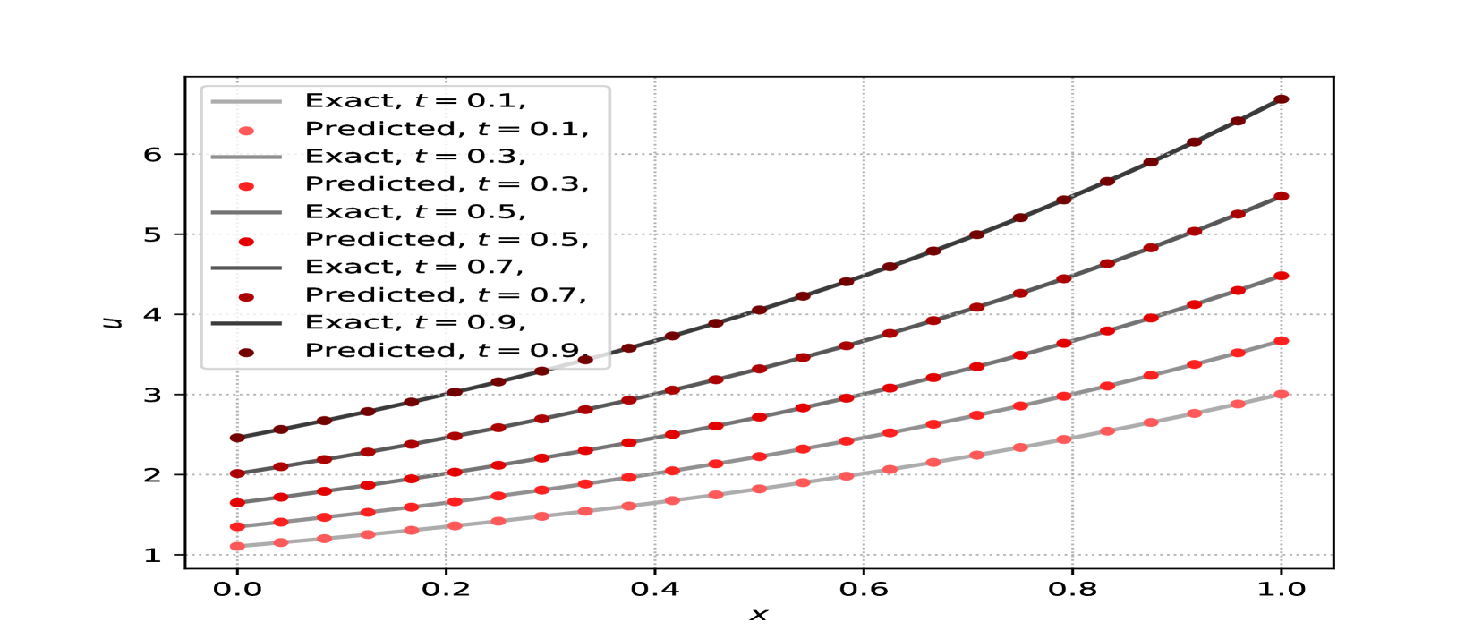
(a) Exact versus prediction at different time $t$

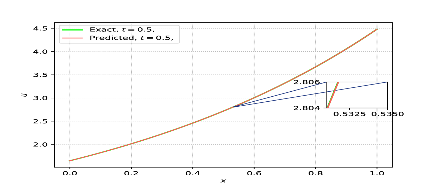
(b) Exact versus prediction at time $t=0.5$

Figure 6: Comparison between exact solution and PINN solution.

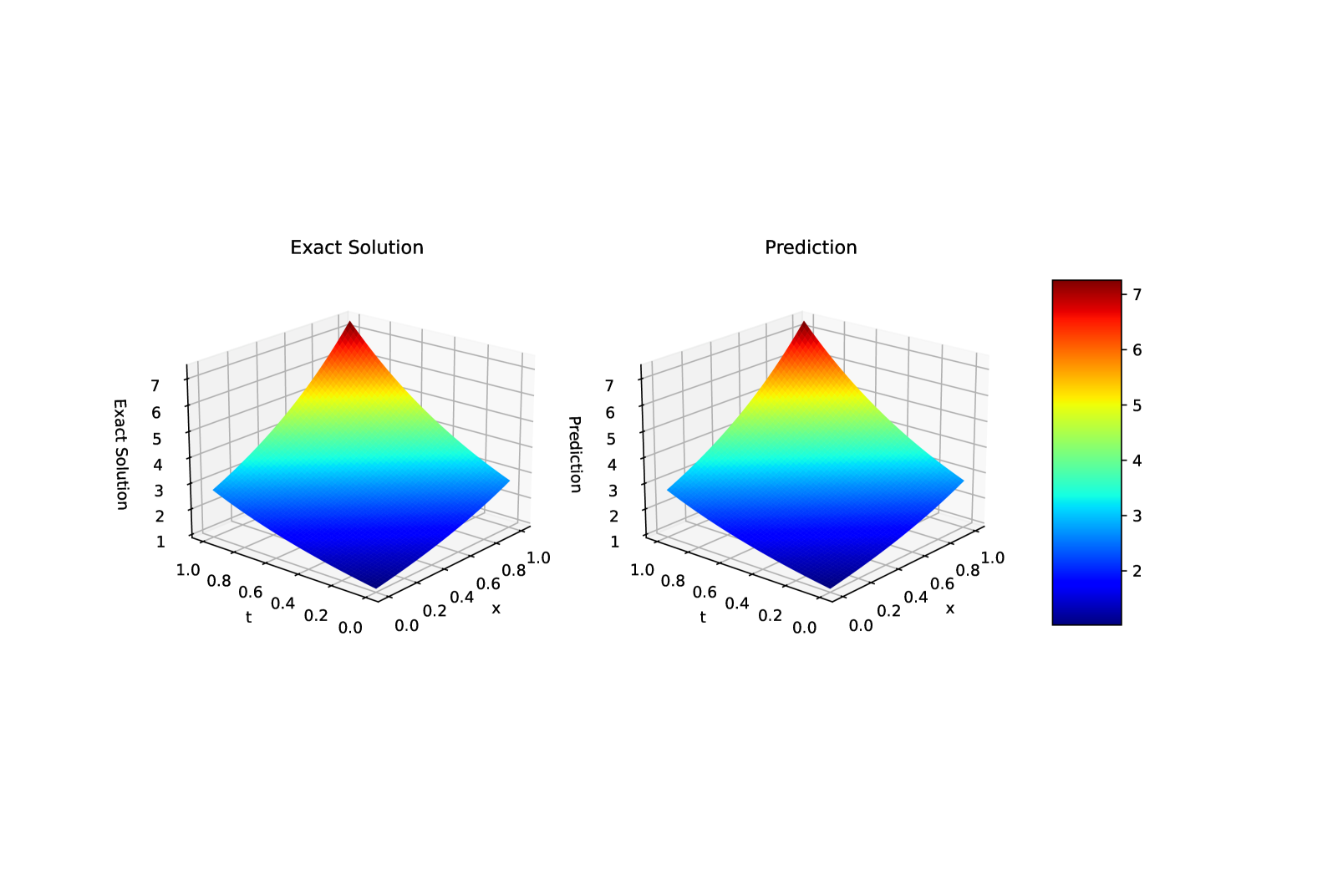
Figure 7: Comparison between exact solution and PINN solution.

$N_{\text{int}}$	$N_{\text{sb}}$	$N_{\text{int}}$	$K-1$	$\bar{d}$	$\lambda$	$\mathcal{E}_{T}$	$\mathcal{E}_{G}^{r}$	Training Time/s
2048	512	512	4	20	0.1	0.0001	8.6e-06	5.6

Table 2: Best-Performing PINN Configuration for Section 3.1.1.

3.1.2 1D nonlinear Burgess equation:

The nonlinear brain tumor growth model proposed in [38, 20] is considered:

$$\frac{\partial u(t,x)}{\partial t}=\frac{1}{2}\frac{\partial^{2}u(t,x)}{\partial x^{2}}+R(t,x),$$ (3.5)

subject to the conditions:

$$u(0,x)=\log(x+2),\quad u(t,0)=\log(t+2),\quad u(t,1)=\log(t+3),$$ (3.6)

where

$$R(t,x)=e^{-u(t,x)}+\frac{1}{2}e^{-2u(t,x)}.$$ (3.7)

The exact solution is:

$$u(t,x)=\log(x+t+2).$$ (3.8)

Figure 8 showcases a graphical comparison between the approximate solutions obtained using PINN and the exact solution for the model given by Eq. (3.5). The results demonstrate that the PINN-based approximation remains highly consistent with the exact solution, highlighting its stability. Moreover, Fig. 8 clearly depicts the increase in tumor cell density as time $t$ progresses. A three-dimensional visualization comparing the PINN and exact solutions is presented in Fig. 9. Additionally, Table 3 provides the relative error $\mathcal{E}_{G}^{r}$ and training error $\mathcal{E}_{T}$ along with the chosen hyper-parameters. A zoom view of the plot at $t=0.5$ reveals that the PINN prediction aligns more closely with the exact solution compared to the Fibonacci and Haar wavelet methods [38].

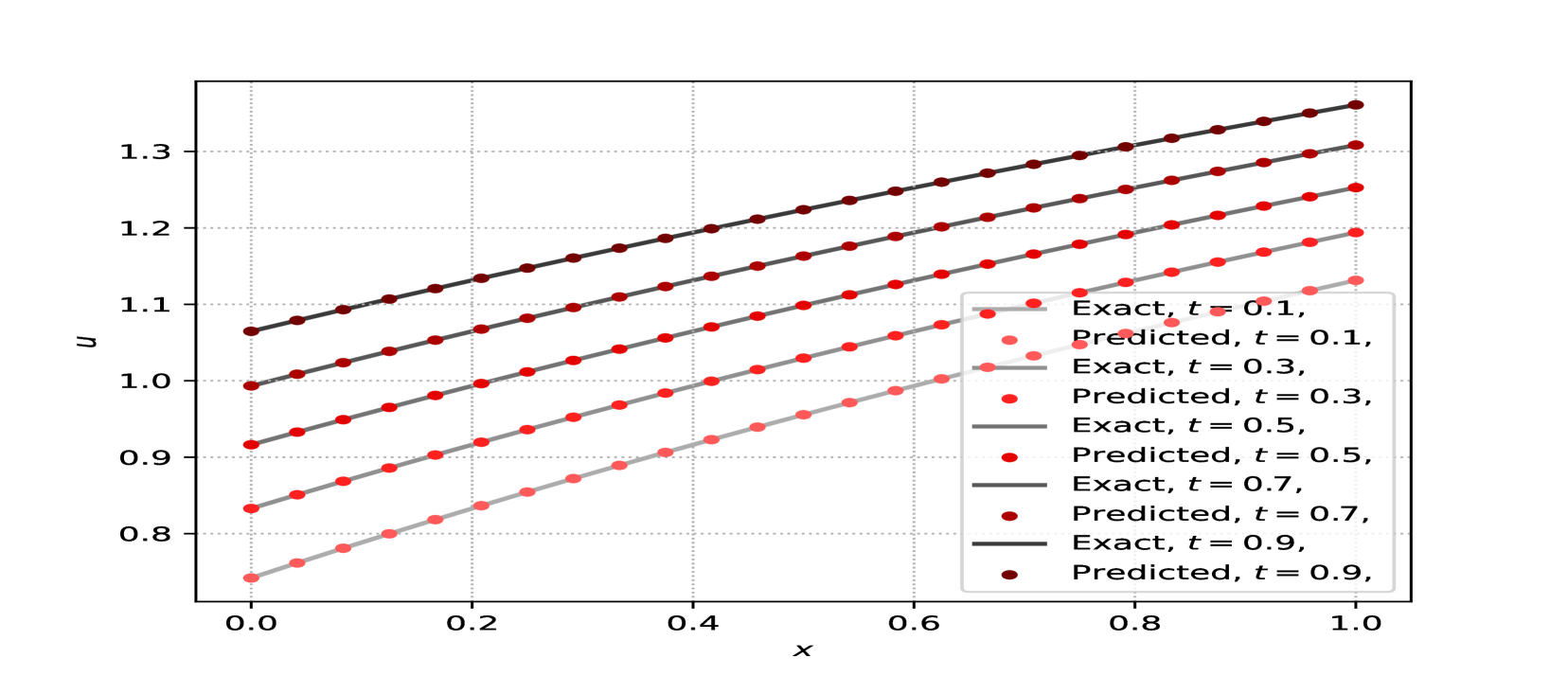
(a) Exact and predicted solution at Different $t$.

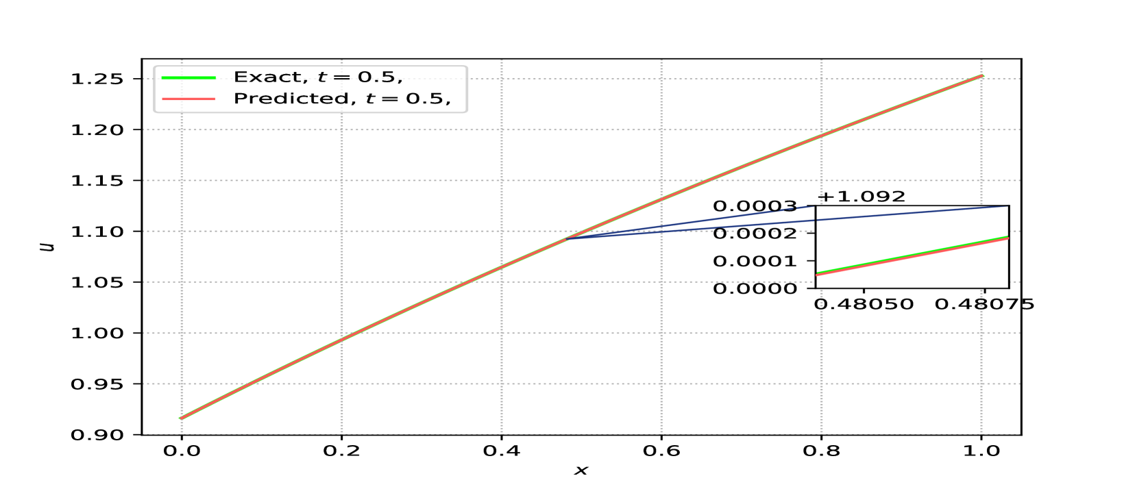
(b) Exact and predicted solution at different $t=0.5$.

Figure 8: Exact and predicted solution.

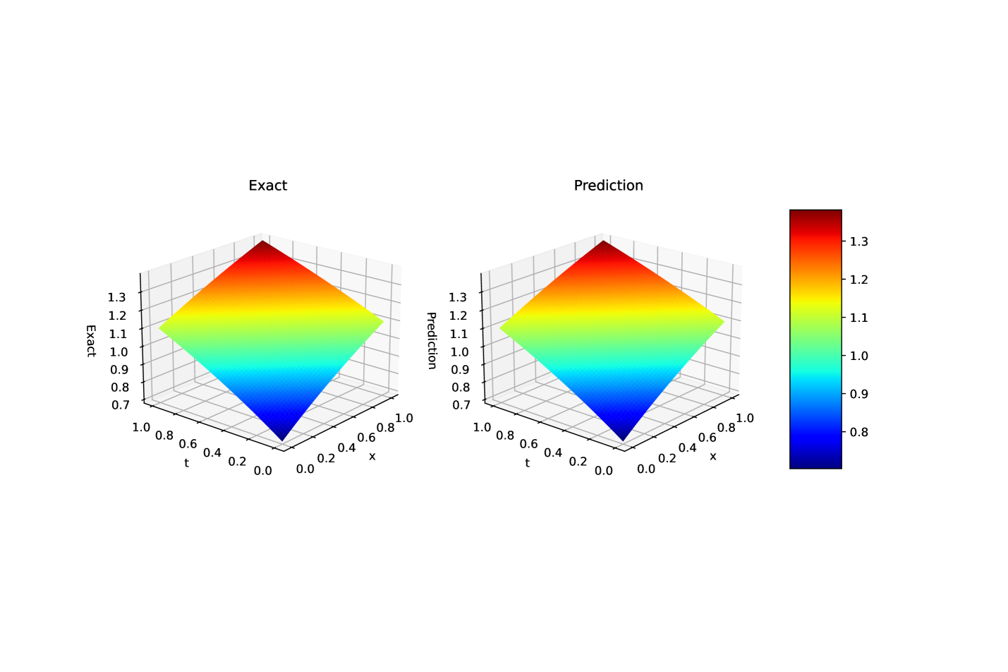
Figure 9: Comparison between exact solution and PINN solution.

$N_{\text{int}}$	$N_{\text{sb}}$	$N_{\text{sb}}$	$K-1$	$\bar{d}$	$\lambda$	$\mathcal{E}_{T}$	$\mathcal{E}_{G}^{r}$	Training Time/s
2048	512	512	4	20	0.1	7.1e-05	2.1e-05	4.9

Table 3: Best-Performing PINN Configuration for Section 3.1.2.

3.1.3 1D nonlinear extended Fisher–Kolmogorov equation

The EFK model in one dimension is expressed as follows:

$$u_{t}+\gamma u_{xxxx}-k_{2}u_{xx}+u^{3}-u =f,$$ (3.9)

$$u(0,x) =\sin(\pi x).$$ (3.10)

$$u(t,0)=0,\quad u(t,1) =0.$$ (3.11)

The analytic solution to this model, as presented in [1] (though with different boundary conditions), is given by $\exp(-t)\sin(\pi x)$. The source term is:

$$\exp(-t)\sin(\pi x)\left(\gamma\pi^{4}+\pi^{2}-2+\exp(-2t)(\sin(\pi x))^{2}\right).$$

Figure 12 shows a graphical comparison between the approximate solutions obtained using PINN and the exact solution. The results demonstrate that the PINN-based approximation closely matches the exact solution, validating its stability. Furthermore, Fig. 17(a) illustrates the variation in tumor cell density over time $t$. Table 4 presents the relative error $\mathcal{E}_{G}^{r}$ and training error $\mathcal{E}_{T}$, along with the selected hyper-parameters.

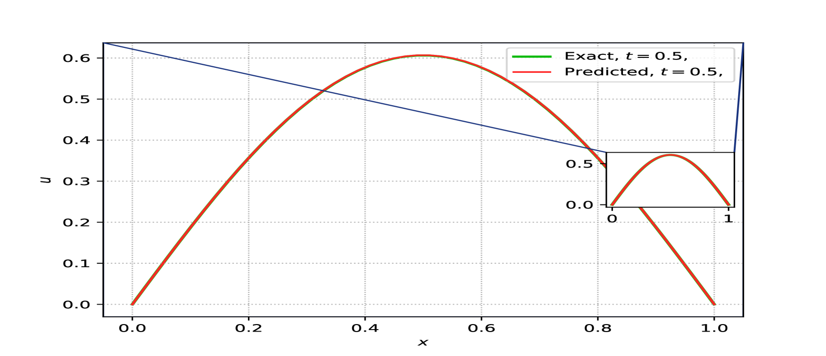
(a) Exact versus predicted solution at different $t=0.5$.

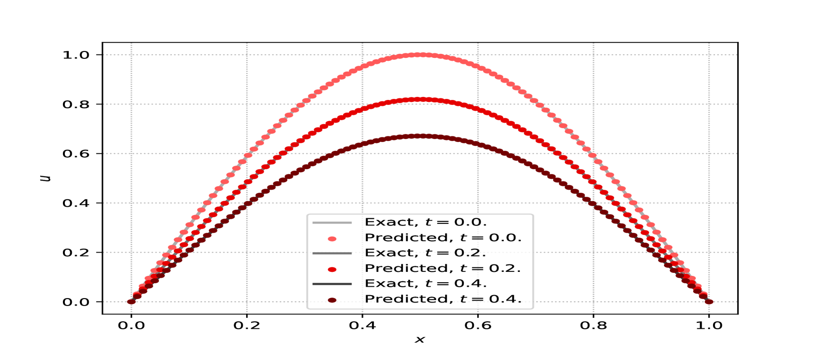
(b) Exact and predicted solution at different t.

Figure 10: Comparison between exact solution and PINN solution at $\gamma=0.0001$.

$N_{\text{int}}$	$N_{\text{sb}}$	$N_{\text{sb}}$	$K-1$	$\bar{d}$	$\lambda$	$\mathcal{E}_{T}$	$\mathcal{E}_{G}^{r}$	Training Time/s
4096	1024	1024	4	20	0.1	0.0003	0.0002	84

Table 4: Best-Performing PINN Configuration for Section 3.1.3.

3.1.4 1D extended Fisher–Kolmogorov equation

Consider the EFK equation:

$$u_{t}+\gamma u_{xxxx}-u_{xx}+u^{3}-u=0,\quad(x,t)\in[0,1]\times(0,T],$$ (3.12)

with initial and boundary conditions:

• $u(x,0)=x^{3}(1-x)^{3}$,

• $u(x,0)=x^{2}(1-x)^{2}$,

$$u(0,t)=0,\quad u(1,t)=0,$$ (3.13)

$$u_{xx}(0,t)=0,\quad u_{xx}(1,t)=0.$$ (3.14)

The numerical solution for this equation has been computed using the parameter $\gamma=0.01$ with different initial values. Figure 11(a) shows the numerical solution for the initial condition $u(x,0)=x^{3}(1-x)^{3}$, while Figure 11(b) corresponds to the initial condition $u(x,0)=x^{2}(1-x)^{2}$. Both figures display the numerical solutions at different times, exhibiting the same characteristics as those presented in [42]. Table 5 reports the training error $\mathcal{E}_{T}$ alongside the chosen hyperparameters.

$N_{\text{int}}$	$N_{\text{sb}}$	$N_{\text{sb}}$	$K-1$	$\bar{d}$	$\lambda$	$\mathcal{E}_{T}$	Training Time/s
2048	512	512	4	20	1	0.0008	36
2048	512	512	4	20	1	0.001	36

Table 5: Best-Performing PINN Configuration for Section 3.1.4.

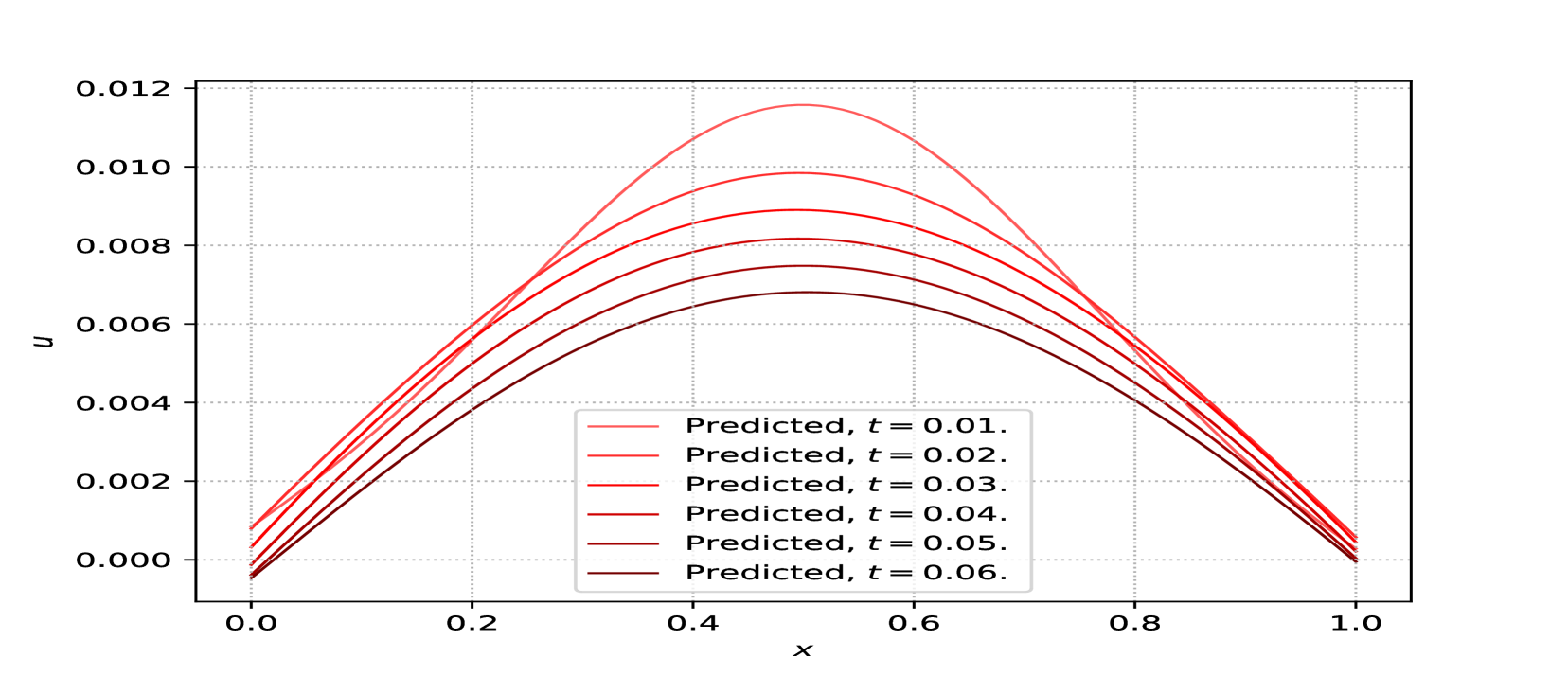
(a) Prediction

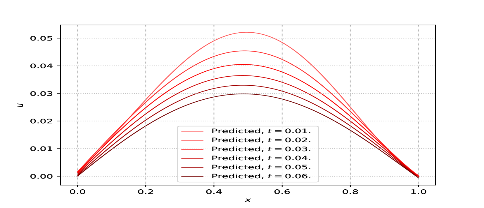
(b) Prediction

Figure 11: Predicted plot with $\gamma=0.01.$

3.1.5 2D extended Fisher–Kolmogorov equation

In this study, we focus on the 2D nonlinear EFK equation.

$$u_{t}+\gamma\Delta^{2}u-\Delta u+u^{3}-u =g(t,x,y)\quad \text{in}\quad(0,T]\times\mathbf{D}$$ (3.15)

$$u(0,x,y) =\sin(\pi x)\sin(\pi y)\quad \text{in}\quad\mathbf{D}$$ (3.16)

$$u =f_{1},\quad\Delta u=f_{2}\quad \text{on}\quad(0,T]\times\partial\mathbf{D}.$$ (3.17)

The exact solution to equation (3.15) is $\sin(\pi x)\sin(\pi y)\exp(-t)$. The source term $g$ can be derive from exact solution. The subsequent plots compare the exact and predicted solutions, shown in both contour and 3D surface formats. Figures 12 and 14 provide graphical comparisons of the approximate solutions obtained using PINN and the exact solution for $\gamma=0.01$, displayed as 3D visualizations at $t=0$ and $t=1$. The results confirm that the PINN-based approximation aligns closely with the exact solution, demonstrating its stability. Additionally, Fig. 14 depicts the contour plot at $t=1$. Table 7 reports the relative error $\mathcal{E}_{G}^{r}$ and training error $\mathcal{E}_{T}$, alongside the chosen hyper-parameters.

(a) Exact

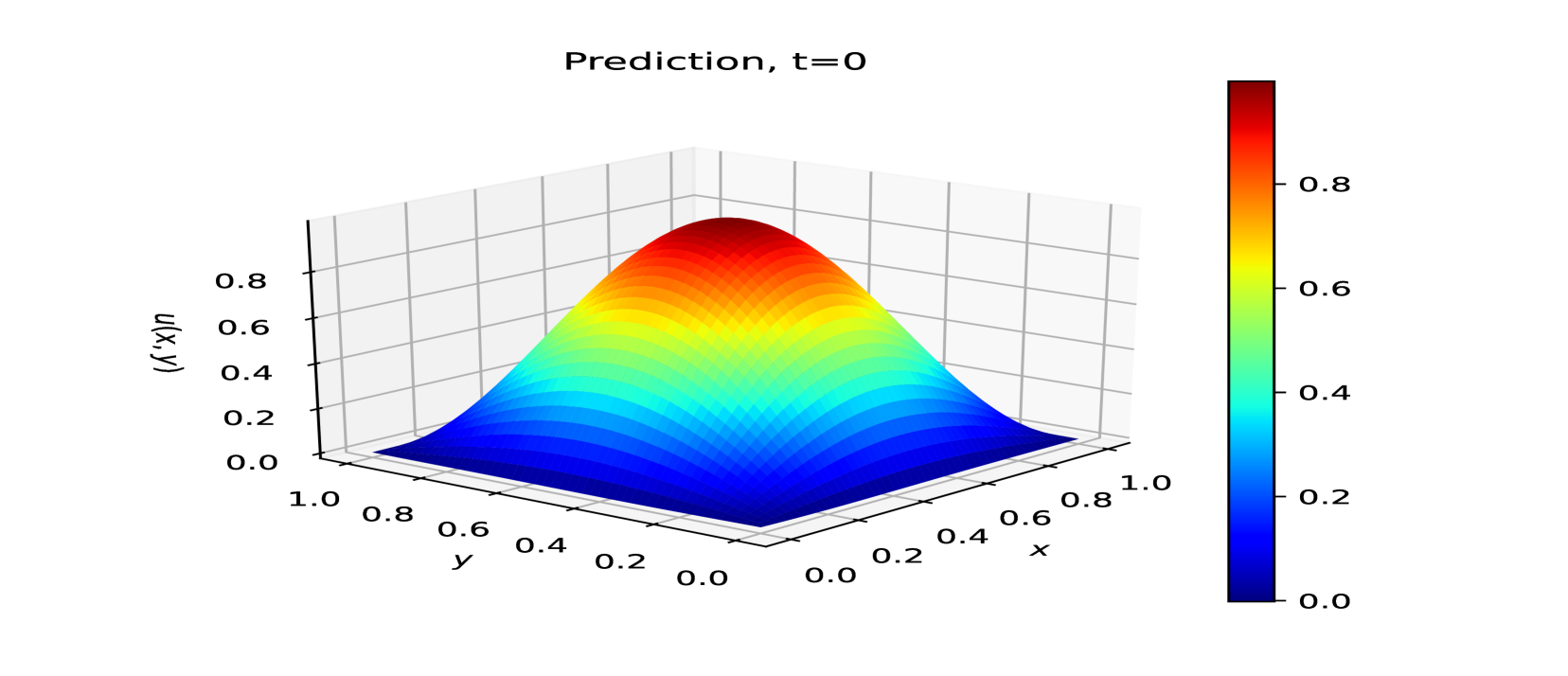
(b) Predicted

Figure 12: Exact and predicted contour plot at $T=0$ with $\gamma=0.01$.

(a) Exact

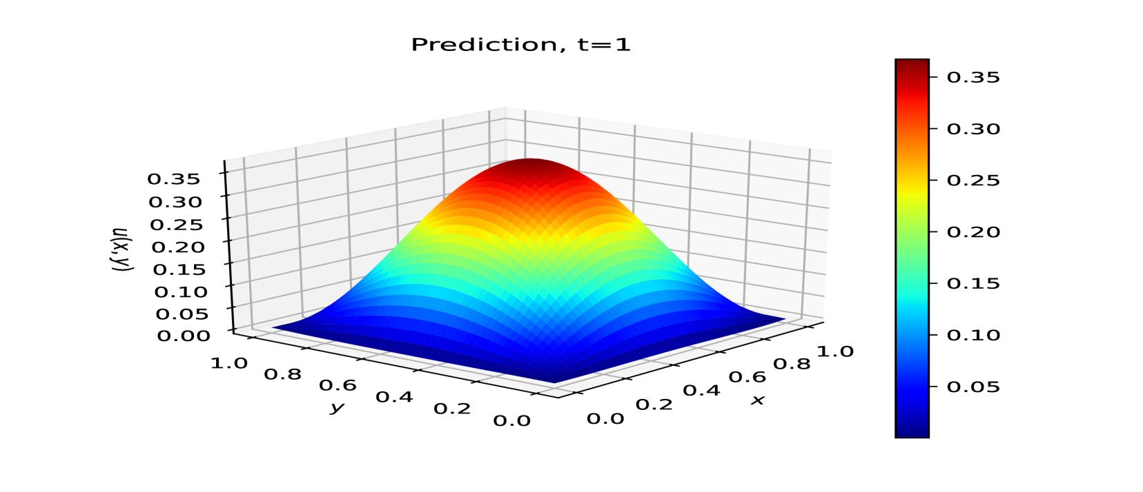
(b) Predicted

Figure 13: Exact and predicted 3D plot at $T=1$ with $\gamma=0.01$.

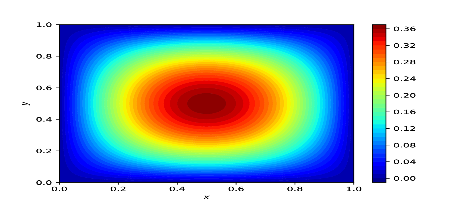
(a) Exact

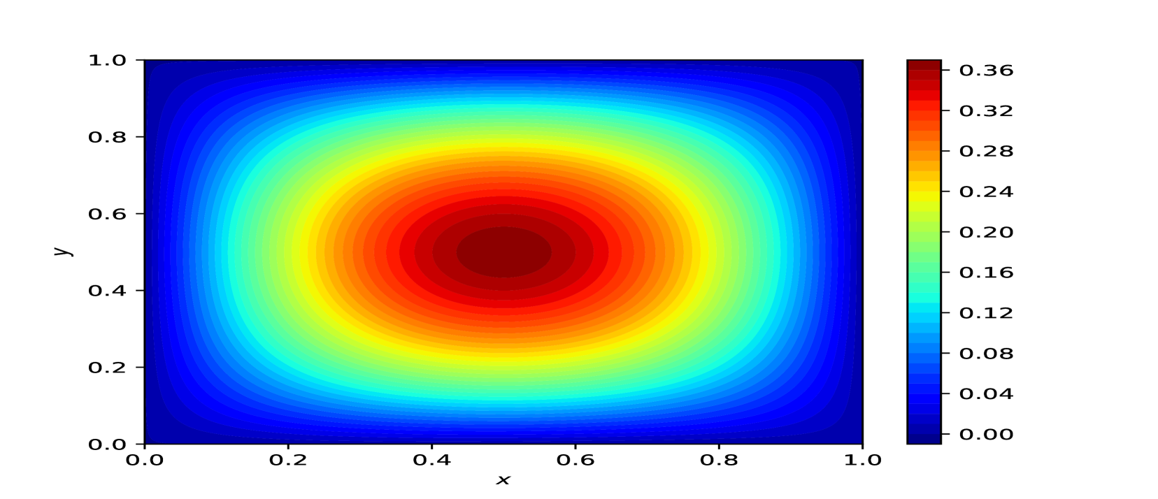
(b) Predicted

Figure 14: Exact and predicted contour plot at $T=1$ with $\gamma=0.01$.

$N_{\text{int}}$	$N_{\text{tb}}$	$N_{\text{sb}}$	$K-1$	$\bar{d}$	$\lambda$	$\mathcal{E}_{T}$	$\mathcal{E}_{G}^{r}$	Training Time/s
8192	2048	2048	4	32	1	0.001	0.0007	650

Table 6: Best-Performing PINN Configuration for Section 3.2.1.

3.2 Inverse Problems

The inverse problems for both models are discussed as follows:

3.2.1 1D linear Burgess equation

The model for linear brain tumor growth given in [38, 20] is analyzed:

$$\frac{\partial u}{\partial t}=\frac{1}{2}\frac{\partial^{2}u}{\partial x^{2}}+u(t,x),$$ (3.18)

subject to the conditions:

$$u(0,x)=x,\quad u(t,0)=0,\quad u(t,1)=e^{t},$$ (3.19)

where in Eq. (2.7), $R(t,x)=u(t,x)$. The exact solution is:

$$u(t,x)=xe^{t}.$$ (3.20)

Figure 15 presents a graphical comparison of the approximate solutions computed using PINN and the exact solution for the model defined by Eq. (3.18). The results confirm that the PINN-based approximation closely matches the exact solution, demonstrating its stability. Furthermore, Fig. 15 illustrates the growth in tumor cell density as time $t$ advances. A three-dimensional representation comparing the PINN and exact solutions is shown in Fig. 16. Additionally, Table 7 reports the relative error $\mathcal{E}_{G}^{r}$ and training error $\mathcal{E}_{T}$ along with the selected hyper-parameters. The zoom view of the plot at $t=0.5$ clearly illustrates that the PINN prediction is closer to the exact solution than the Fibonacci and Haar wavelet methods [38].

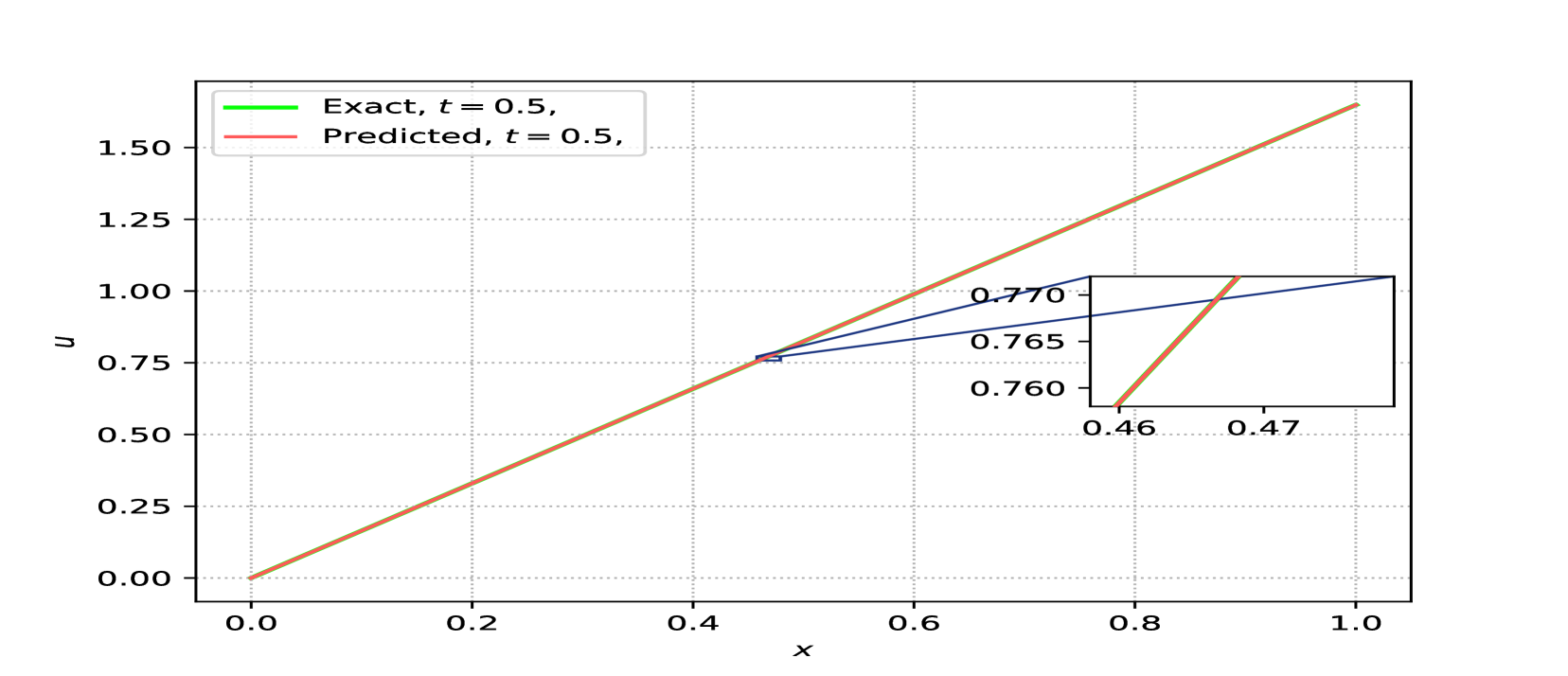
(a) Exact and predicted solution at $t=0.5$.

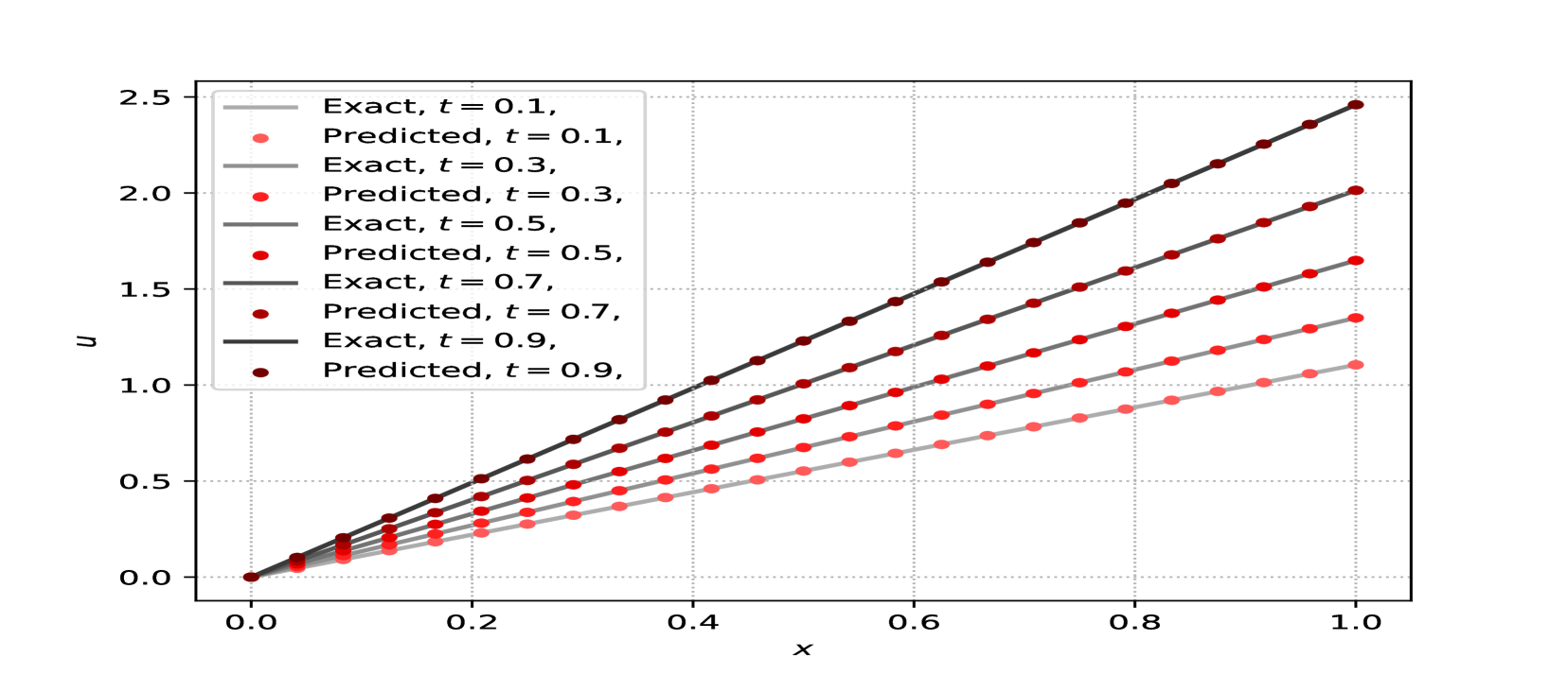
(b) Exact and predicted solution at different t.

Figure 15: Exact and predicted solution of model.

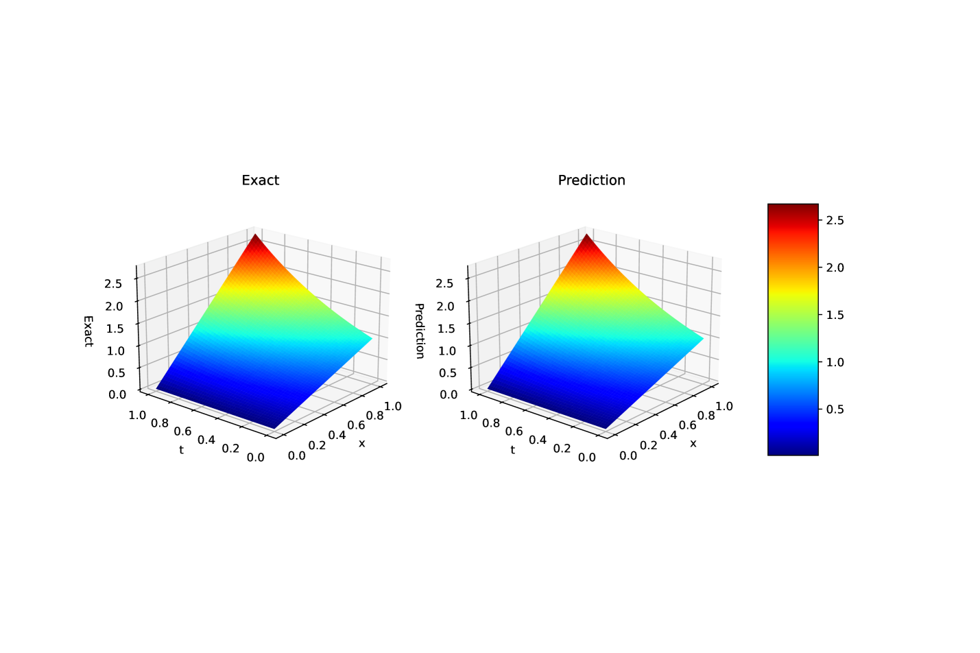
Figure 16: Exact and predicted surface plot.

$N$	$K-1$	$\bar{d}$	$\lambda$	$\mathcal{E}_{T}$	$\mathcal{E}_{G}^{r}$	Training Time/s
3072	4	16	0.1	0.0004	3.9e-05	4

Table 7: Best-Performing PINN Configuration for Section 3.2.1.

3.2.2 1D extended Fisher–Kolmogorov equation

The 1D case of the EFK model is given as follows:

$$u_{t}+\gamma u_{xxxx}-u_{xx}+u^{3}-u=f,$$ (3.21)

The exact solution [1]is :

$$u(t,x)=\exp{(-t)}\sin(\pi x).$$ (3.23)

The corresponding source term is:

$$f(t,x)=\exp{(-t)}\sin(\pi x)\left(\gamma\pi^{4}+\pi^{2}-2+\exp(-2t)(\sin(\pi x))^{2}\right).$$

Figure 17 presents a graphical comparison of the approximate solutions obtained using PINN and the exact solution for the model represented by Eq. (3.23). The results indicate that the PINN-based approximation aligns closely with the exact solution, validating its stability. Additionally, Fig. 17(a) illustrates the variation in tumor cell density over time $t$. A three-dimensional visualization comparing the PINN and exact solutions is provided in Fig. 17(b). Furthermore, Table 8 presents the relative error $\mathcal{E}_{G}^{r}$ and training error $\mathcal{E}_{T}$ alongside the chosen hyper-parameters.

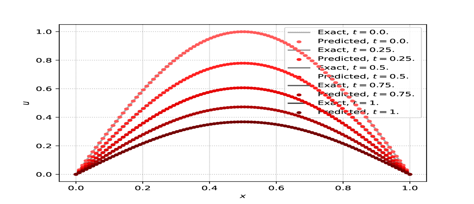
(a) Exact and Predicted solution at different t

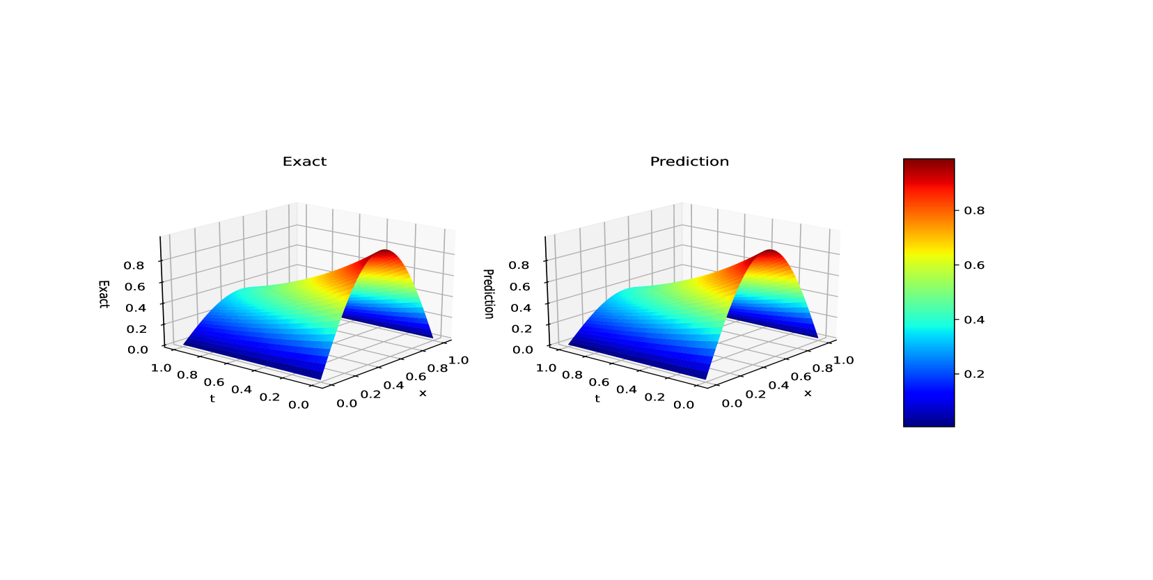
(b) Exact and Predicted surface plot

Figure 17: Exact and predicted solution of model at $\gamma=0.0001$.

$N$	$K-1$	$\bar{d}$	$\lambda$	$\mathcal{E}_{T}$	$\mathcal{E}_{G}^{r}$	Training Time (s)
6144	4	20	0.1	0.0008	0.0002	60

Table 8: Best-Performing PINN Configuration for Section 3.2.2.

3.2.3 2D extended Fisher–Kolmogorov equation:

The 2D equation has following exact solution [3][24] :

$$\exp({-t})\exp\left(-\frac{(x-0.5)^{2}}{\beta}-\frac{(y-0.5)^{2}}{\beta}\right).$$

The source term is derived from the exact solution. The model is solved for different parameter values over time. Both the exact and predicted solutions are presented in contour and 3D surface formats, as shown in the following sub-figures. Figures 18, 19, and 20 present a graphical comparison of the approximate solutions obtained using PINN and the exact solution for varying values of $\beta$, displayed as contour plots and 3D visualizations. The results show that the PINN-based approximation closely matches the exact solution, confirming its stability. Additionally, Fig. 17(a) illustrates the changes in tumor cell density over time $t$. Table 9 reports the relative error $\mathcal{E}_{G}^{r}$ and training error $\mathcal{E}_{T}$ along with the selected hyper-parameters.

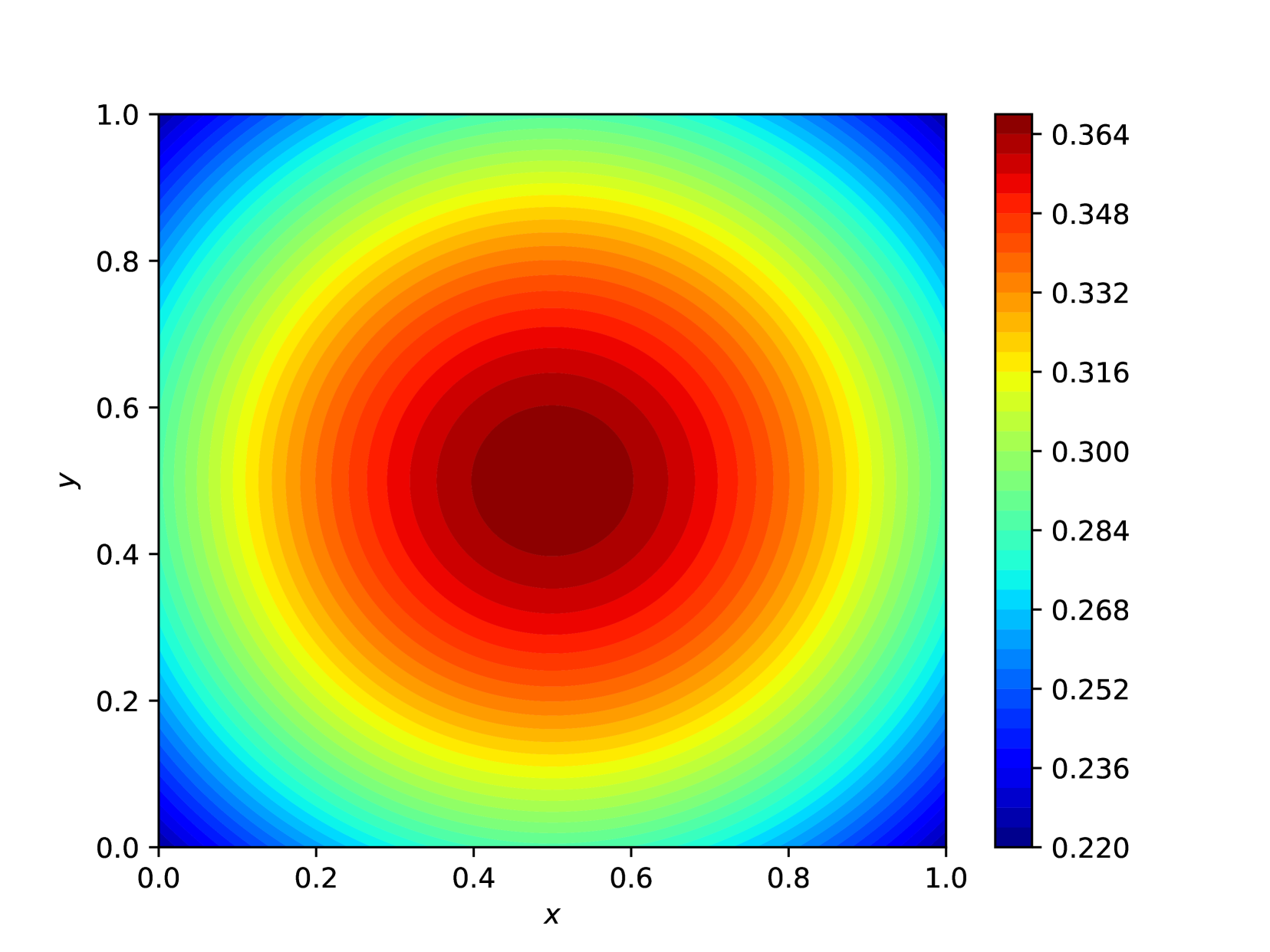
(a) Exact

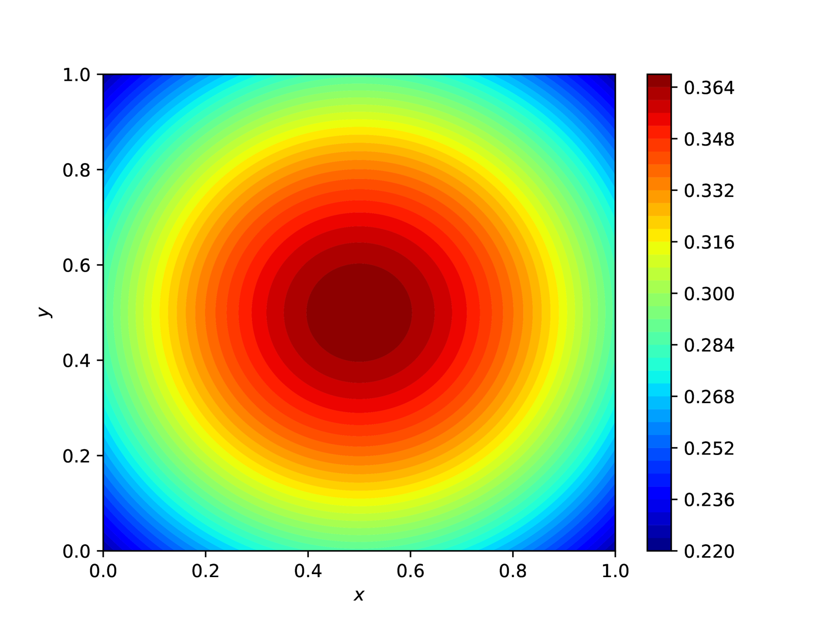
(b) Predicted

(c) Exact

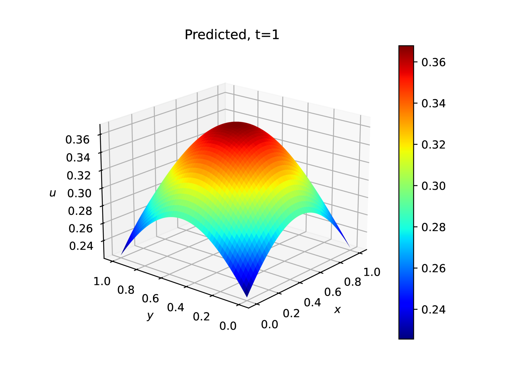
(d) Predicted

Figure 18: The exact and predicted solutions at $T=1$, with $\gamma=0.0001$ and $\beta=1$.

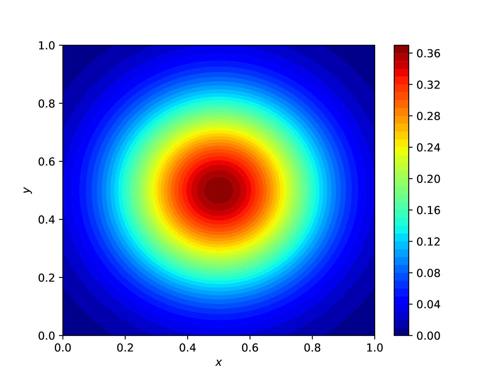
(a) Exact

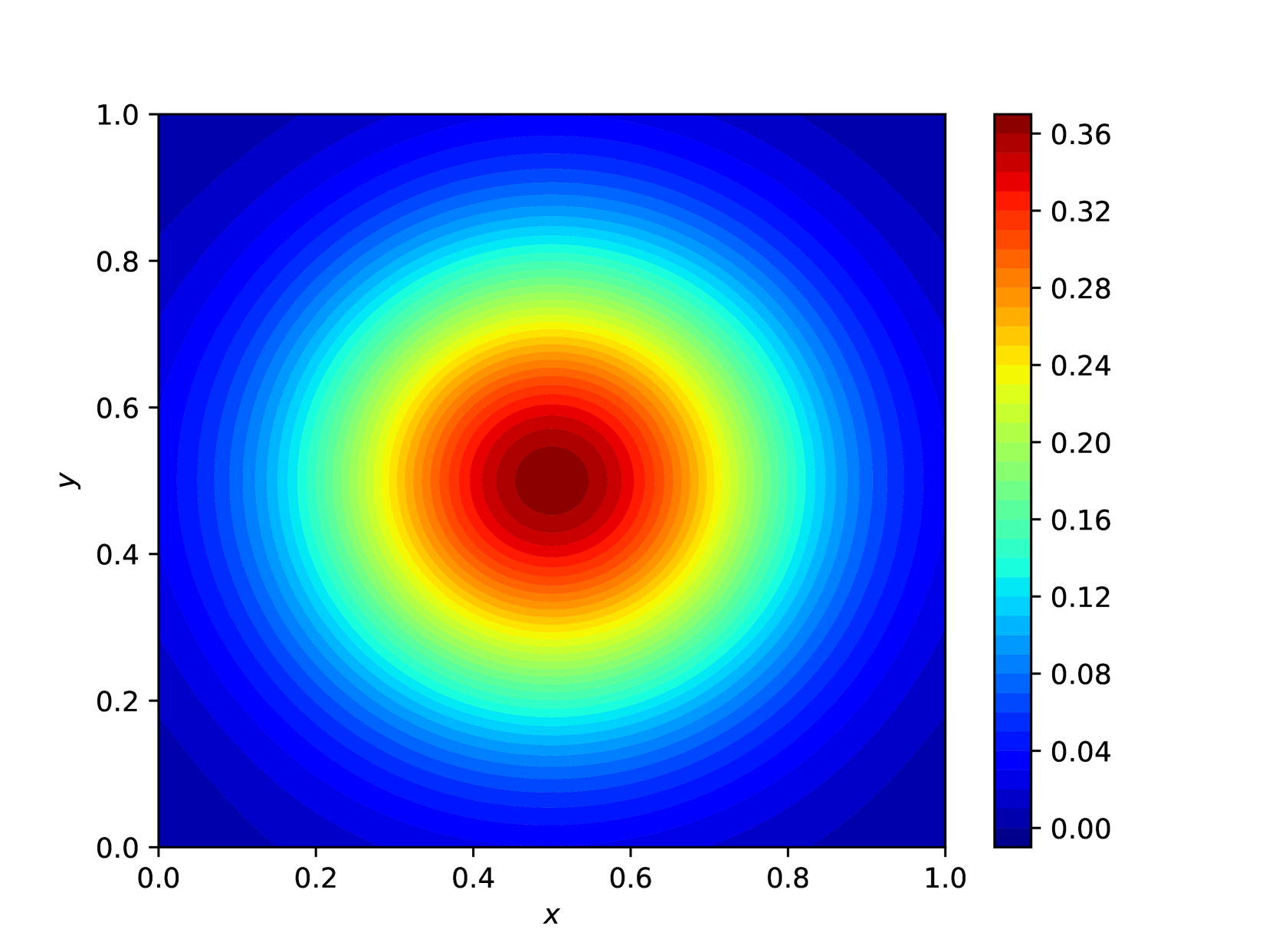
(b) Predicted

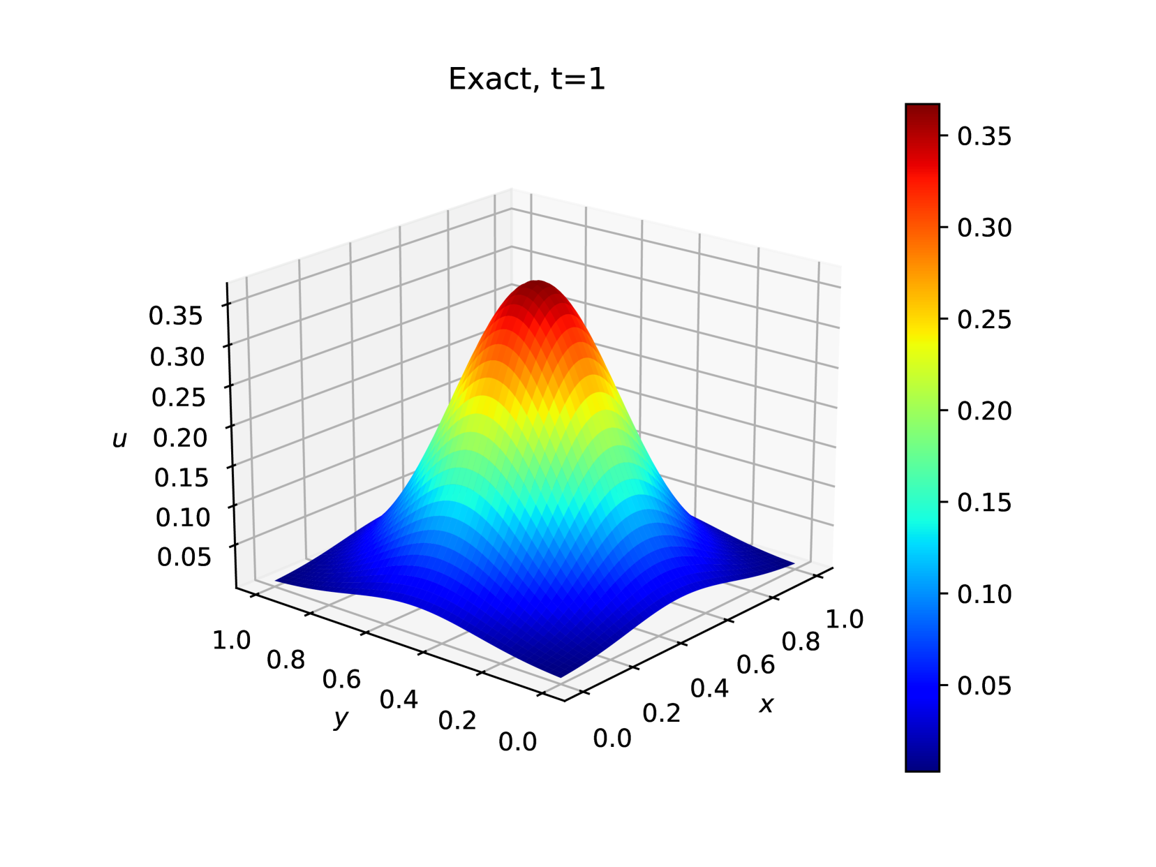
(c) Exact

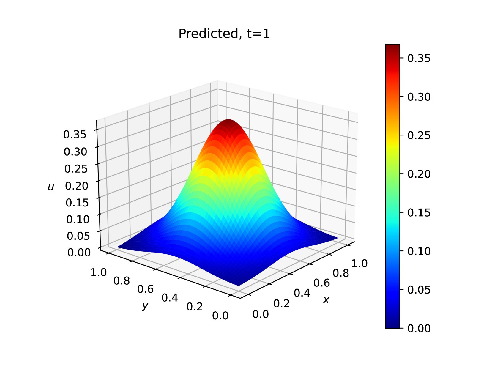
(d) Predicted

Figure 19: The exact and predicted solutions at $T=1$, with $\gamma=0.0001$ and $\beta=0.1$.

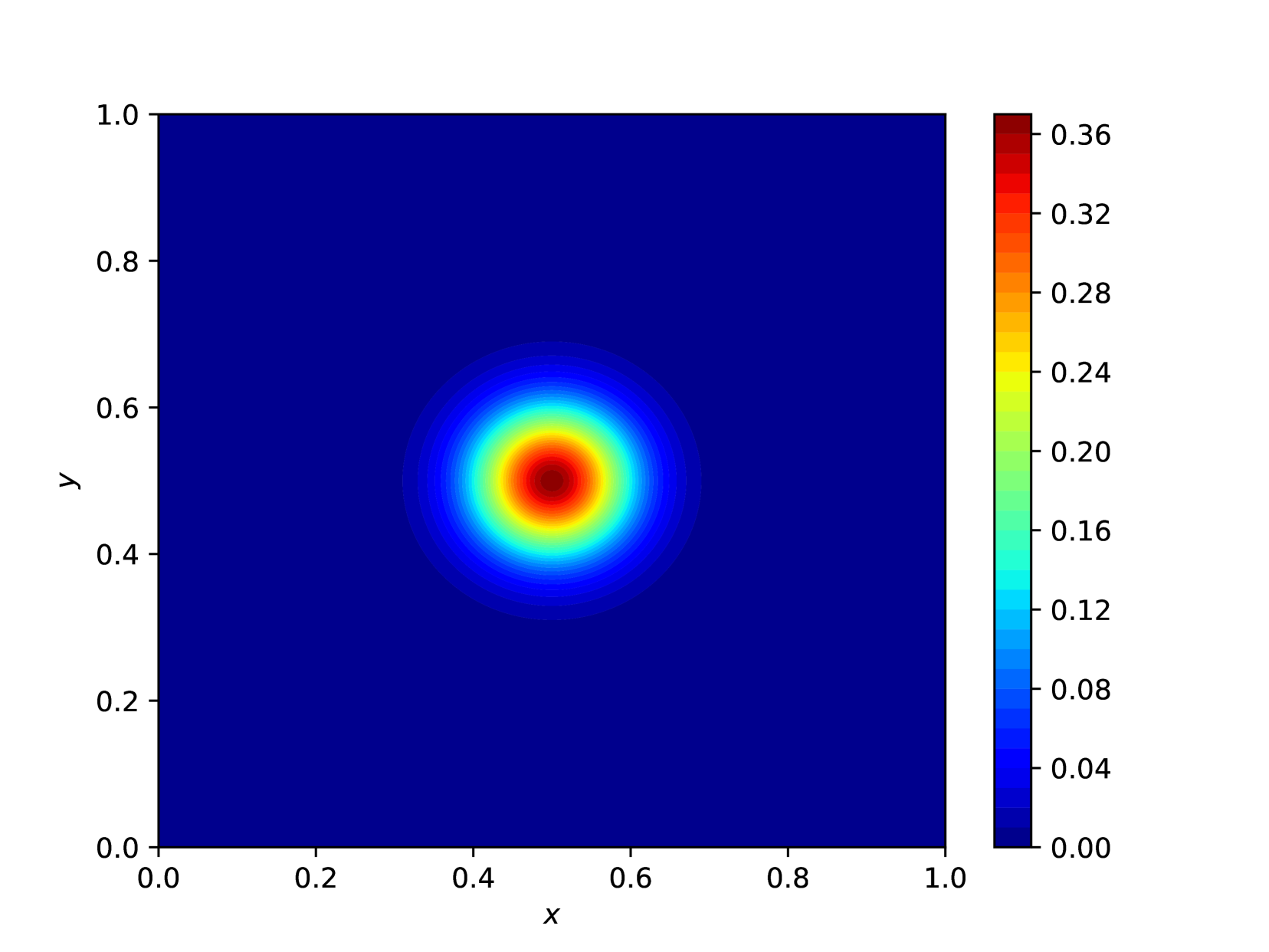
(a) Exact

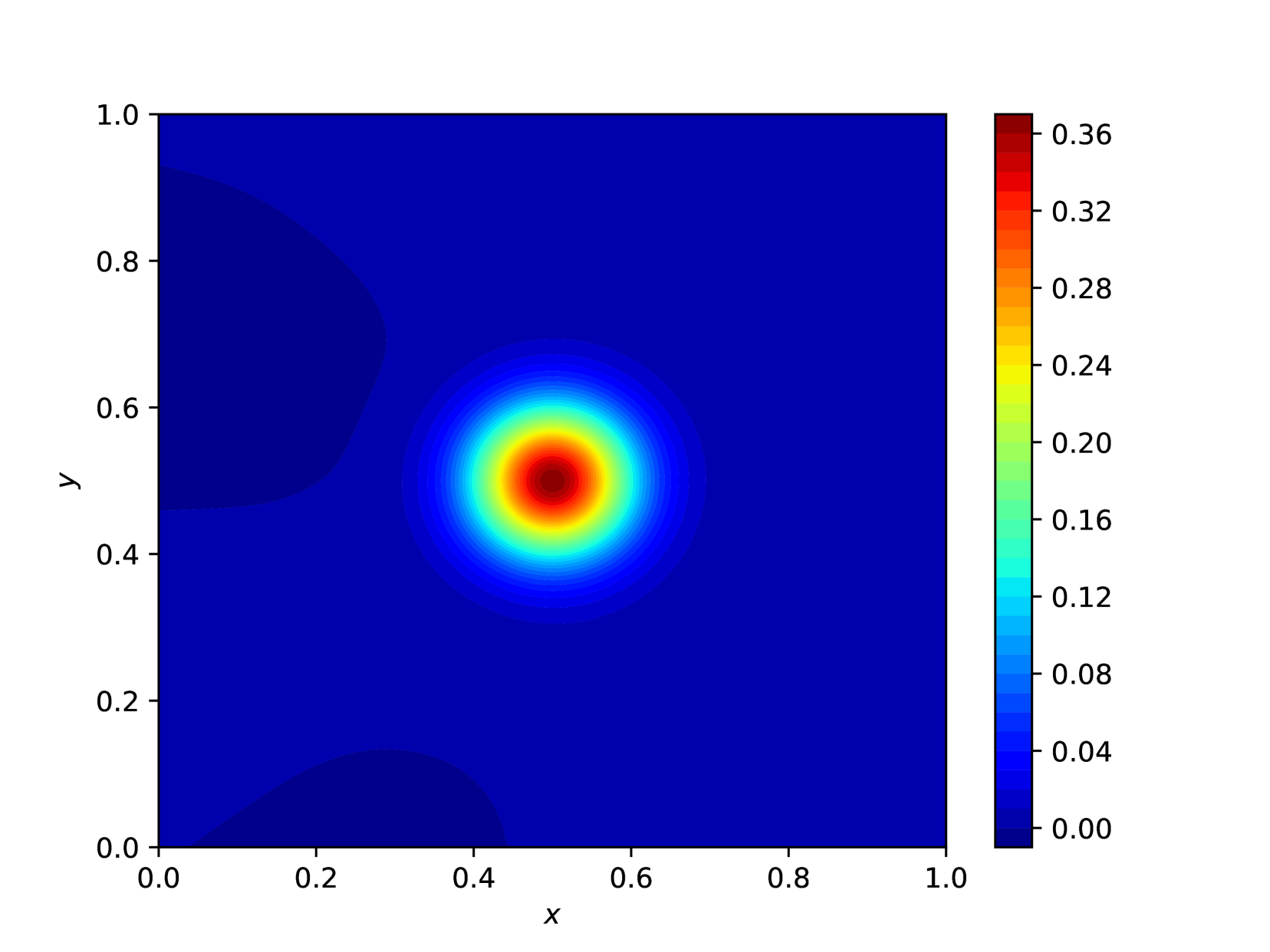
(b) Predicted

(c) Exact

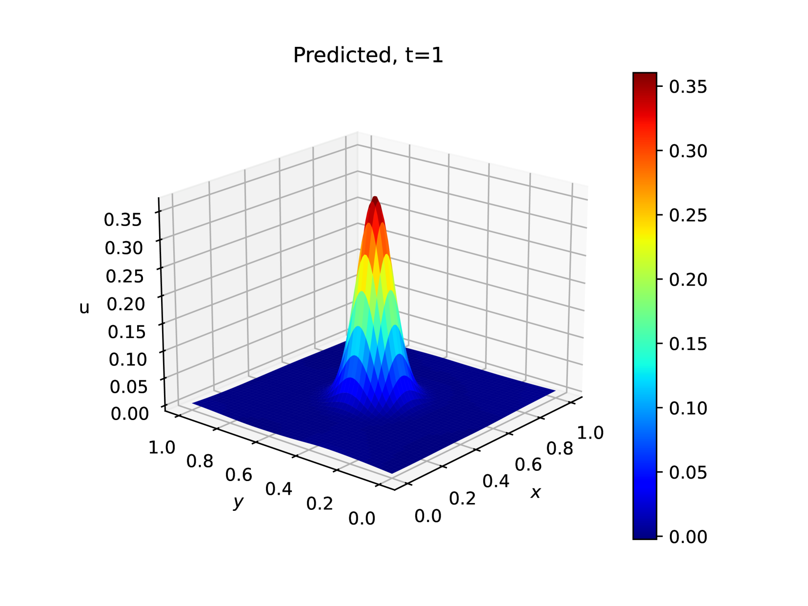
(d) Predicted

Figure 20: The exact and predicted solutions at $T=1$, with $\gamma=0.0001$ and $\beta=0.01.$

$\beta$	$N$	$K-1$	$\bar{d}$	$\lambda$	$\mathcal{E}_{T}$	$\mathcal{E}_{G}^{r}$	Training Time (sec.)
1	12288	4	24	0.1	0.0003	0.0002	550
0.1	12288	4	36	1	0.002	0.0009	700
0.01	6144	4	42	1	0.02	0.01	483

Table 9: Best-Performing PINN Configuration for Section 3.2.3.

4 Discussions

This section presents the statistical analysis of the first and last experiments, conducted using RStudio software. Figures 21 and 22 provide an overall comparison. Figures 22(a), 21(b) and 21(c) illustrate the variation in training error, $L^{2}$ error and relative $L^{2}$ error, respectively, across different neuron counts (12, 16, 20 and 24) over multiple LBFGS iterations (500, 1000 and 5000). Outliers are highlighted with red circles in the $L^{2}$ and relative $L^{2}$ error plots. Additionally, Figure 21(d) presents a bar plot comparing the $L^{2}$ and relative $L^{2}$ errors for the best-performing configuration, corresponding to the maximum LBFGS iterations (5000). These visualizations provide insights into training behavior, error convergence, and the impact of hyperparameter selection. Similarly, Figures 22(a), 22(b) and 22(c) depict the variation in training error, $L^{2}$ error and relative $L^{2}$ error for the last experiment, considering neuron counts of 16, 20, 24 and 28 over the same LBFGS iterations. Outliers are again highlighted with red circles in the $L^{2}$ and relative $L^{2}$ error plots. Figure 22(d) presents a bar plot comparing the $L^{2}$ and relative $L^{2}$ errors for the best-performing configuration at 5000 LBFGS iterations. These visualizations facilitate the analysis of training behavior, error convergence, and the influence of hyperparameter selection across experiments. The analysis highlights how the number of neurons affects different error types. Increasing the LBFGS iterations leads to error reduction. Notably, an outlier in the relative error $\mathcal{E}_{G}^{r}$ is observed at 500 LBFGS iterations for different neuron counts.

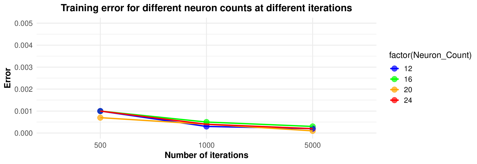
(a) Training error of 3.1.1 with varying neuron counts and different L-BFGS iterations.

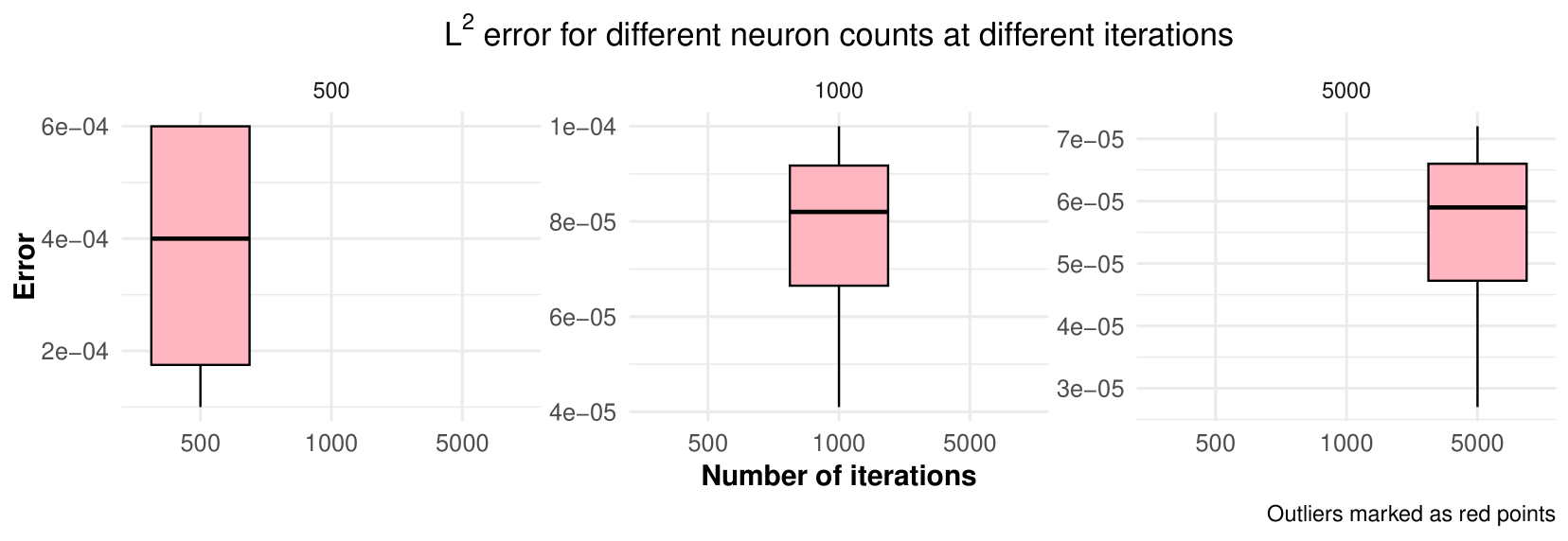
(b) L² error of numerical experiment 3.1.1 with 12, 16, 20, and 24 neurons and varying L-BFGS iterations.

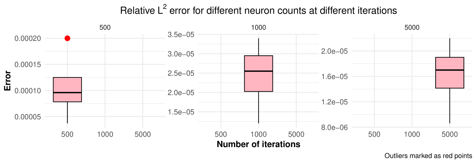
(c) L² relative error of numerical experiment 3.1.1 with 12, 16, 20, and 24 neurons and varying L-BFGS iterations.

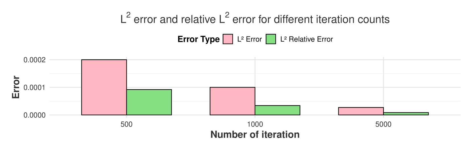
(d) Bar plot of $L^{2}$ error and relative $L^{2}$ error for numerical experiment 3.1.1 with different L-BFGS iterations under the best hyperparameter configuration.

Figure 21: Statistical measure of errors for numerical experiment 3.1.1.

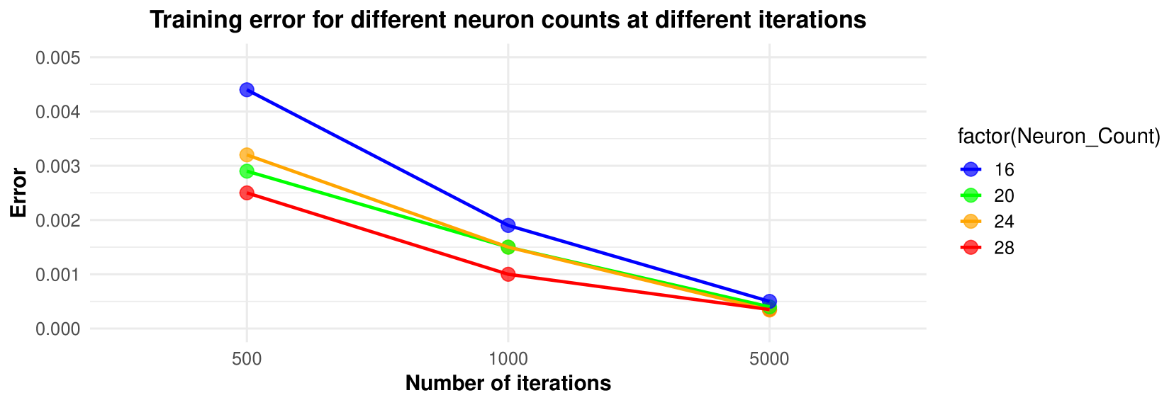
(a) Training error of numerical experiment 3.2.3 for $\beta=1$ with different neuron counts and varying L-BFGS iterations

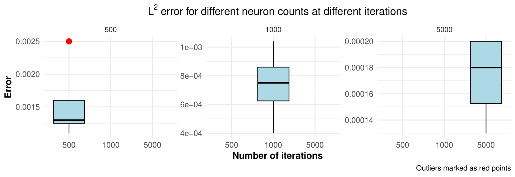
(b) L² error of numerical experiment 3.2.3 for $\beta=1$, with 16, 20, 24, and 28 neurons and varying L-BFGS iterations.

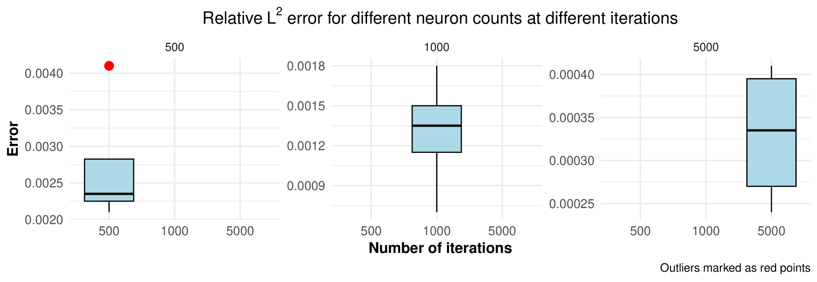
(c) Relative L² error of numerical experiment 3.2.3 for $\beta=1$, with 16, 20, 24, and 28 neurons and varying L-BFGS iterations.

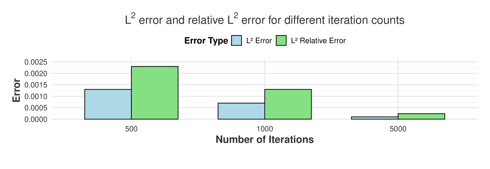
(d) Bar plot of $L^{2}$ error and relative $L^{2}$ error for numerical experiment 3.2.3 with $\beta=1$, using different L-BFGS iterations under the best hyperparameter configuration.

Figure 22: Statistical measure of errors for numerical experiment 3.2.3 with $\beta=1$.

5 Conclusion

This paper presents Physics-Informed Neural Networks (PINNs) for approximating solutions to partial differential equations in the modeling of low-grade brain tumors. The approach involves training a neural network to approximate classical solutions by minimizing the residuals of the governing PDE. Both well-posed problems (with initial and boundary conditions) and ill-posed problems (without complete initial or boundary data) are considered, using a gradient-based optimization method. Theoretical error bounds for the PINN approximation are derived, and both forward and inverse numerical experiments are conducted to demonstrate the effectiveness of PINNs in solving linear and nonlinear PDEs efficiently. Glioblastoma is a frequently occurring malignant brain tumor in adults, characterized by rapid progression and an unfavorable prognosis. Standard treatment typically involves a combination of surgery, radiation therapy, and chemotherapy. In recent years, mathematical modeling has played a crucial role in studying brain tumors under both treated and untreated conditions. This study presents a mathematical model for glioblastoma, integrating key factors of tumor growth: cancer cell diffusion and proliferation rates. The PINN method was applied to obtain numerical solutions for the nonlinear biharmonic EFK equation, which arises in brain tumor dynamics, as well as the Burgesss equation. A comparison with other mesh-less local weak-form methods demonstrated that the PINN Algorithm effectively solves forward and inverse nonlinear fourth-order PDEs, particularly the EFK equation and the first-order Burgesss equation relevant to brain tumor modeling. The results strongly correlate with established exact solutions, while graphical and tabular analyses indicate that the advanced PINNs method achieves superior accuracy in brain tumor modeling, exceeding traditional computational techniques. We derive rigorous error bounds for PINNs and perform numerical experiments to assess their accuracy in solving both linear and nonlinear equations. Additionally, we establish the convergence and reliability of the neural network.

Declaration of competing interest

The authors declare that they have no competing interests.

Appendix

An estimate for the generalization error of the given equation is derived for forward problems.

Appendix E.1.

Let $u\in C^{2}(\mathbf{D}\times[0,T])$ be the unique classical solution of the Burgess equation (2.7), where the source term $R$ satisfies Lipchitz condition (Appendix E.6). Consider $u^{\ast}=u_{\theta^{\ast}}$, a PINN approximation obtained through Algorithm 2.1, corresponding to the loss functions (2.31) and (2.32). Then, the generalization error (2.34) satisfies the following bound:

$$\bm{\mathcal{E}}_{G}\leqslant C_{1}\left(\bm{\mathcal{E}}_{T}^{tb}+\bm{\mathcal{E}}_{T}^{int}+C_{2}(\bm{\mathcal{E}}_{T}^{sb})^{\frac{1}{2}}+(C_{quad}^{tb})^{\frac{1}{2}}N_{tb}^{-\frac{\alpha_{tb}}{2}}+(C_{quad}^{int})^{\frac{1}{2}}N_{int}^{-\frac{\alpha_{int}}{2}}+C_{2}(C_{quad}^{sb})^{\frac{1}{4}}N_{sb}^{-\frac{\alpha_{sb}}{4}}\right),$$ (5.1)

where the constants are given by:

$$C_{1} =\sqrt{T+(1+2C_{R})T^{2}e^{(1+2C_{R})T}},\quad C_{2}=\sqrt{C_{\partial\mathbf{D}}(u,u^{\ast})T^{\frac{1}{2}}},$$ (5.2)

$$C_{\partial\mathbf{D}} =0.5|\partial\mathbf{D}|^{\frac{1}{2}}\left(\|u\|_{C^{1}([0,T]\times\partial\mathbf{D})}+\|u^{\ast}\|_{C^{1}([0,T]\times\partial\mathbf{D})}\right).$$

The constants $C_{quad}^{tb}=C_{quad}^{tb}(\|\mathfrak{R}^{2}_{tb,\theta^{\ast}}\|_{C^{2}})$, $C_{quad}^{sb}=C_{quad}^{tb}(\|\mathfrak{R}^{2}_{sb,\theta^{\ast}}\|_{C^{2}})$, and $C_{quad}^{int}=C_{quad}^{int}(\|\mathfrak{R}^{2}_{int,\theta^{\ast}}\|_{C^{0}})$ arise from the quadrature error.

Proof.

The proof follows the approach of [35] (see Theorem 3.1). The authors briefly discuss a related argument in [46]. ∎

Appendix E.2.

Consider $u\in C^{4}\left([0,1]\times[0,T]\right)$ as the unique solution to the EFK (2.10). Let $u^{\ast}=u_{\theta^{\ast}}$ be the Physics-Informed Neural Network (PINN) approximation obtained using Algorithm 2.1. The non linear term $F(u)$ satisfied the Lipchitz condition Appendix E.7. Then, the generalization error (2.34) satisfies the following bound:

$$\bm{\mathcal{E}}_{G}\leqslant C_{1}\left(\bm{\mathcal{E}}_{T}^{tb}+\bm{\mathcal{E}}_{T}^{int}+C_{2}(\bm{\mathcal{E}}_{T}^{sb})^{\frac{1}{2}}+(C_{quad}^{tb})^{\frac{1}{2}}N_{tb}^{-\frac{\alpha_{tb}}{2}}+(C_{quad}^{int})^{\frac{1}{2}}N_{int}^{-\frac{\alpha_{int}}{2}}+C_{2}(C_{quad}^{sb})^{\frac{1}{4}}N_{sb}^{-\frac{\alpha_{sb}}{4}}\right),$$ (5.3)

where:

• $\bm{\mathcal{E}}_{G}$ denotes the generalization error.

• $\bm{\mathcal{E}}_{T}^{tb}$, $\bm{\mathcal{E}}_{T}^{sb}$, and $\bm{\mathcal{E}}_{T}^{int}$ are the errors associated with the temporal boundary, spatial boundary, and interior points, respectively.

• The constants are defined as:

  $$C_{1} =\sqrt{(T+2T^{2}C_{3}e^{2C_{3}T})},$$

  $$C_{3} =\sqrt{\gamma(\|u\|_{C^{2}_{x}}+\|u^{\ast}\|_{C^{2}_{x}})^{2}+(\|u\|_{C^{2}_{x}}+\|u^{\ast}\|_{C^{2}_{x}})+\frac{1}{2}+C_{E}},$$

  $$C_{2} =\sqrt{8\gamma(\|u\|_{C^{3}_{x}}+\|u^{\ast}\|_{C^{3}_{x}})T^{1/2}}.$$

• The quadrature error constants are:

  $$C_{quad}^{tb} =C_{quad}^{tb}(\|\mathfrak{R}^{2}_{tb,\theta^{\ast}}\|_{C^{4}}),$$

  $$C_{quad}^{sb} =C_{quad}^{sb}(\|\mathfrak{R}^{2}_{sb,\theta^{\ast}}\|_{C^{2}}),$$

  $$C_{quad}^{int} =C_{quad}^{int}(\|\mathfrak{R}^{2}_{int,\theta^{\ast}}\|_{C^{0}}).$$

• $N_{tb}$, $N_{sb}$, and $N_{int}$ represent the number of training points for the temporal boundary, spatial boundary, and interior domain, respectively.

Proof.

Let $\bar{u}:u^{\ast}-u$.
We can write the residual of EFK equation (2.29) in the following form:

$$\bar{u}_{t}+\gamma\bar{u}_{xxxx}-\bar{u}_{xx}+F(u^{\ast}-u)=\mathfrak{R}_{int},$$ (5.4)

$$\text{where}~x\in(0,1)~\text{and}~t\in(0,T),$$

$$\bar{u}(x,0)=\mathfrak{R}_{tb}~\text{where}~x\in(0,1),$$

$$\bar{u}(0,t)=\mathfrak{R}_{sb_{1}}~\text{where}~t\in(0,T),$$

$$\bar{u}(1,t)=\mathfrak{R}_{sb_{2}}~\text{where}~t\in(0,T),$$

$$\bar{u}_{xx}(0,t)=\mathfrak{R}_{sb_{3}}~\text{where}~t\in(0,T),$$

$$\bar{u}_{xx}(1,t)=\mathfrak{R}_{sb_{4}}~\text{where}~t\in(0,T).$$

We can write

$$\bar{u}\bar{u}_{xxxx}=(\bar{u}\bar{u}_{xxx})_{x}-(\bar{u}_{x}\bar{u}_{xx})_{x}+(\bar{u}_{xx})^{2}$$ (5.5)

We denote $\mathfrak{R}_{int}=\mathfrak{R}_{int,\theta^{\ast}},\mathfrak{R}_{tb}=\mathfrak{R}_{tb,\theta^{\ast}},\mathfrak{R}_{sb_{i}}=\mathfrak{R}_{sb,\theta^{\ast}}~\text{where}~i=0~\text{to}~4$ Multipyling the eq (5.4) by $\bar{u}$ and integrating over $(0,1),$ we get

$$\frac{1}{2}\frac{d}{dt}\int_{0}^{1}\bar{u}^{2}\,dx+\gamma\int_{0}^{1}\bar{u}\bar{u}_{xxxx}\,dx-\int_{0}^{1}\bar{u}\bar{u}_{xx}\,dx+\int_{0}^{1}\bar{u}F(u^{\ast}-u)\,dx=\int_{0}^{1}\bar{u}\mathfrak{R}_{int}\,dx.$$ (5.6)

$$\frac{1}{2}\frac{d}{dt}\int_{0}^{1}\bar{u}^{2}\,dx =-\gamma\int_{0}^{1}\bar{u}\bar{u}_{xxxx}\,dx+\int_{0}^{1}\bar{u}\bar{u}_{xx}\,dx-\int_{0}^{1}\bar{u}F(u^{\ast}-u)\,dx+\int_{0}^{1}\mathfrak{R}_{int}\bar{u}\,dx.$$ (5.7)

Now putting the value of $\bar{u}\bar{u}_{xxxx}$ from (5.5), we get

$$\frac{1}{2}\frac{d}{dt}\int_{0}^{1}\bar{u}^{2}\,dx=-\gamma\bar{u}\bar{u}_{xxx}\mid_{0}^{1}+\gamma\bar{u}_{x}\bar{u}_{xx}\mid_{0}^{1}-\gamma\int\limits_{0}^{1}\bar{u}_{xx}^{2}dx+\int\limits_{0}^{1}\bar{u}\bar{u}_{xx}dx+\int_{0}^{1}\bar{u}F(u^{\ast}-u)\,dx+\int_{0}^{1}\mathfrak{R}_{int}\bar{u}\,dx.$$ (5.8)

$$\frac{1}{2}\frac{d}{dt}\int_{0}^{1}\bar{u}^{2}\,dx \leqslant\gamma\|\bar{u}\|_{C_{x}^{3}}\left(|\mathfrak{R}_{sb_{1}}|+|\mathfrak{R}_{sb_{2}}|+|\mathfrak{R}_{sb_{3}}|+|\mathfrak{R}_{sb_{4}}|\right)+\gamma\left(\|\bar{u}\|_{C^{2}_{x}}\right)^{2}\int_{0}^{1}1\,dx+\|\bar{u}\|_{C^{2}_{x}}\int_{0}^{1}\bar{u}\,dx$$

$$\quad+\frac{1}{2}\int_{0}^{1}\mathfrak{R}_{int}^{2}\,dx+\left(\frac{1}{2}+C_{E}\right)\int_{0}^{1}\bar{u}^{2}\,dx.$$ (5.9)

$$\frac{1}{2}\frac{d}{dt}\int_{0}^{1}\bar{u}^{2}\,dx\leqslant\gamma\parallel\bar{u}\parallel_{C_{x}^{3}}\left(|\mathfrak{R}_{sb_{1}}|+|\mathfrak{R}_{sb_{2}}|+|\mathfrak{R}_{sb_{3}}|+|\mathfrak{R}_{sb_{4}}|\right)+\left(\gamma(\|\bar{u}\|_{C^{2}_{x}})^{2}+\|\bar{u}\|_{C^{2}_{x}}+\frac{1}{2}+C_{E}\right)\left(\int_{0}^{1}\bar{u}^{2}dx\right)+\frac{1}{2}\int_{0}^{1}\mathfrak{R}_{int}^{2}dx.$$ (5.10)

$$\frac{1}{2}\frac{d}{dt}\int_{0}^{1}\bar{u}^{2}\,dx \leqslant\gamma(\|u\|_{C^{3}_{x}}+\|u^{\ast}\|_{C^{3}_{x}})\left(|\mathfrak{R}_{sb_{1}}|+|\mathfrak{R}_{sb_{2}}|+|\mathfrak{R}_{sb_{3}}|+|\mathfrak{R}_{sb_{4}}|\right)$$

$$\quad+\left(\gamma(\|u\|_{C^{2}_{x}}+\|u^{\ast}\|_{C^{2}_{x}})^{2}+(\|u\|_{C^{2}_{x}}+\|u^{\ast}\|_{C^{2}_{x}})+\frac{1}{2}+C_{E}\right)\int_{0}^{1}\bar{u}^{2}\,dx$$

$$\quad+\frac{1}{2}\int_{0}^{1}\mathfrak{R}_{int}^{2}\,dx.$$ (5.11)

$$\frac{1}{2}\frac{d}{dt}\int_{0}^{1}\bar{u}^{2}\,dx\leqslant C_{1}\sum\limits_{i}^{4}\left(\mathfrak{R}_{sb_{i}}\right)+C_{2}\int_{0}^{1}\bar{u}^{2}dx\quad +\frac{1}{2}\int_{0}^{1}\mathfrak{R}_{int}^{2}\,dx.$$ (5.12)

The mixed norm is defined as

$$\|u\|_{C^{m}_{t}C^{n}_{x}}.$$

Then, integrating the above inequality over $[0,\bar{T}]$ for any $\bar{T}\leqslant T$, and using the Cauchy-Schwarz and Gronwall’s inequalities, we obtain the following estimate:

$$\int\limits_{0}^{1}\bar{u}^{2}\,dx \leqslant\int\limits_{0}^{1}\mathfrak{R}_{tb}^{2}\,dx+2C_{1}\bar{T}^{\frac{1}{2}}\sum\limits_{i=1}^{4}\left(\int\limits_{0}^{T}\mathfrak{R}^{2}_{sb_{i}}\,dt\right)^{\frac{1}{2}}$$

$$\quad+\int\limits_{0}^{T}\int\limits_{0}^{1}\mathfrak{R}_{int}^{2}\,dx\,dt+2C_{2}\int\limits_{0}^{T}\int\limits_{0}^{1}\bar{u}^{2}\,dx\,dt.$$ (5.13)

$$\int\limits_{0}^{1}\bar{u}^{2}\,dx \leqslant(1+2TC_{2}e^{2C_{2}T})\left[\int\limits_{0}^{1}\mathfrak{R}_{tb}^{2}dx+8C_{1}T^{\frac{1}{2}}\sum\limits_{i}^{4}\left(\int\limits_{0}^{T}\mathfrak{R}^{2}_{sb_{i}}dt\right)^{\frac{1}{2}}\right]$$

$$+(1+2\bar{T}C_{2}e^{2C_{2}T})\left[2\int\limits_{0}^{T}\int\limits_{0}^{1}\mathfrak{R}_{int}^{2}dxdt+2C_{2}\int\limits_{0}^{T}\int\limits_{0}^{1}\bar{u}^{2}dxdt\right].$$ (5.14)

Again integrating over $T$ we get,

$$\bm{\mathcal{E}}_{G} \leqslant(T+2T^{2}C_{2}e^{2C_{2}T})\left[\int\limits_{0}^{1}\mathfrak{R}_{tb}^{2}dx+8C_{1}T^{\frac{1}{2}}\sum\limits_{i}^{4}\left(\int\limits_{0}^{T}\mathfrak{R}^{2}_{sb_{i}}dt\right)^{\frac{1}{2}}\right]$$

$$+(\bar{T}+2T^{2}C_{2}e^{2C_{2}T})\left[2\int\limits_{0}^{\bar{T}}\int\limits_{0}^{1}\mathfrak{R}_{int}^{2}dxdt+2C_{2}\int\limits_{0}^{T}\int\limits_{0}^{1}\bar{u}^{2}dxdt\right],$$ (5.15)

where $C_{1}=\left(\gamma(\|u\|_{C^{3}_{x}}+\|u^{\ast}\|_{C^{3}_{x}})\right)$ and $C_{2}=\left(\gamma(\|u\|_{C^{2}_{x}}+\|u^{\ast}\|_{C^{2}_{x}})^{2}+(\|u\|_{C^{2}_{x}}+\|u^{\ast}\|_{C^{2}_{x}})+\frac{1}{2}+C_{E}\right)$ . ∎

Appendix E.3Proof of Theorem 2.6.

Consider the EFK equation:

$$\partial_{t}U^{n}-\Delta W^{n}=F(U^{n}),\quad x\in\mathbf{D},\ t>0,$$ (5.16)

where

$$W^{n}=k_{2}U^{n}-k_{1}\Delta U^{n},$$ (5.17)

with Neumann boundary conditions:

$$\frac{\partial U^{n}}{\partial n}=0,\quad\frac{\partial W^{n}}{\partial n}=0,\quad x\in\partial\mathbf{D},$$ (5.18)

and the initial condition:

$$U^{n}(x,0)=U^{n}_{0}(x).$$ (5.19)

The nonlinear term is given by

$$F(U^{n})=(U^{n})^{3}-U^{n}.$$ (5.20)

Taking the $L^{2}$ inner product of the first equation with $U^{n}$, we obtain:

$$\int_{\mathbf{D}}\partial_{t}U^{n}\cdot U^{n}\,dx-\int_{\mathbf{D}}\Delta W^{n}\cdot U^{n}\,dx=\int_{\mathbf{D}}F(U^{n})\cdot U^{n}\,dx.$$ (5.21)

Using the identity

$$\int_{\mathbf{D}}\partial_{t}U^{n}\cdot U^{n}\,dx=\frac{1}{2}\frac{d}{dt}\|U^{n}\|_{L^{2}(\mathbf{D})}^{2},$$ (5.22)

we obtain

$$\frac{1}{2}\frac{d}{dt}\|U^{n}\|_{L^{2}(\mathbf{D})}^{2}-\int_{\mathbf{D}}\Delta W^{n}\cdot U^{n}\,dx=\int_{\mathbf{D}}F(U^{n})\cdot U^{n}\,dx.$$ (5.23)

Using integration by parts and the Neumann boundary conditions,

$$\int_{\mathbf{D}}\Delta W^{n}\cdot U^{n}\,dx=-\int_{\mathbf{D}}\nabla W^{n}\cdot\nabla U^{n}\,dx.$$ (5.24)

Substituting $W^{n}=k_{2}U^{n}-\gamma\Delta U^{n}$ gives

$$\nabla W^{n}=k_{2}\nabla U^{n}-\gamma\nabla\Delta U^{n}.$$ (5.25)

Taking the inner product with $\nabla U^{n}$,

$$\int_{\mathbf{D}}\nabla W^{n}\cdot\nabla U^{n}\,dx=k_{2}\|\nabla U^{n}\|_{L^{2}(\mathbf{D})}^{2}-\gamma\int_{\mathbf{D}}\nabla\Delta U^{n}\cdot\nabla U^{n}\,dx.$$ (5.26)

Using integration by parts,

$$\int_{\mathbf{D}}\nabla\Delta U^{n}\cdot\nabla U^{n}\,dx=-\|\Delta U^{n}\|_{L^{2}(\mathbf{D})}^{2}.$$ (5.27)

Thus,

$$\int_{\mathbf{D}}\nabla W^{n}\cdot\nabla U^{n}\,dx=k_{2}\|\nabla U^{n}\|_{L^{2}(\mathbf{D})}^{2}+\gamma\|\Delta U^{n}\|_{L^{2}(\mathbf{D})}^{2}.$$ (5.28)

Substituting back,

$$\frac{1}{2}\frac{d}{dt}\|U^{n}\|_{L^{2}(\mathbf{D})}^{2}+k_{2}\|\nabla U^{n}\|_{L^{2}(\mathbf{D})}^{2}+\gamma\|\Delta U^{n}\|_{L^{2}(\mathbf{D})}^{2}=\int_{\mathbf{D}}F(U^{n})U^{n}\,dx.$$ (5.29)

For $F(U^{n})=(U^{n})^{3}-U^{n}$,

$$\int_{\mathbf{D}}F(U^{n})U^{n}\,dx=\int_{\mathbf{D}}((U^{n})^{4}-(U^{n})^{2})\,dx.$$ (5.30)

Using $(U^{n})^{4}\leqslant c_{0}(U^{n})^{2}$ for some $c_{0}$, we obtain

$$\int_{\mathbf{D}}F(U^{n})U^{n}\,dx\leqslant c_{0}\|U^{n}\|_{L^{2}(\mathbf{D})}^{2}.$$ (5.31)

Thus,

$$\frac{1}{2}\frac{d}{dt}\|U^{n}\|_{L^{2}(\mathbf{D})}^{2}+\gamma\|\Delta U^{n}\|_{L^{2}(\mathbf{D})}^{2}\leqslant c_{0}\|U^{n}\|_{L^{2}(\mathbf{D})}^{2}.$$ (5.32)

Applying Grönwall’s inequality,

$$\|U^{n}\|_{L^{2}(\mathbf{D})}^{2}+\gamma\int_{0}^{T}\|\Delta U^{n}\|_{L^{2}(\mathbf{D})}^{2}\,d\tau\leqslant\|U^{n}(0)\|_{L^{2}(\mathbf{D})}^{2}\exp(2c_{0}T).$$ (5.33)

Thus, $\{U^{n}\}$ is uniformly bounded in $C([0,T];H^{2}(\mathbf{D}))$. Define the energy functional:

$$E(U^{n})=\int_{\mathbf{D}}\left(\frac{\gamma}{2}|\Delta U^{n}|^{2}+\frac{1}{2}|\nabla U^{n}|^{2}+\frac{1}{4}(1-(U^{n})^{2})^{2}\right)dx.$$ (5.34)

Form Theorem 2.4

$$\frac{d}{dt}E(U^{n})\leqslant 0.$$ (5.35)

Since $E(U^{n})$ is non-increasing, it follows that

$$E(U^{n})\leqslant E(U^{n})\leqslant C(U^{n}(0)).$$ (5.36)

Thus,

$$\|\nabla U^{n}\|_{L^{2}(\mathbf{D})}^{2}+\|\Delta U^{n}\|_{L^{2}(\mathbf{D})}^{2}+2\int_{\mathbf{D}}F(U^{n})dx\leqslant C(U^{n}(0)).$$ (5.37)

By the Sobolev embedding theorem, this implies the uniform bound:

$$\|U^{n}(t)\|_{\infty}\leqslant C^{\prime},\quad\forall t\in[0,T].$$ (5.38)

$$\frac{\partial U^{n}}{\partial t}+\gamma\Delta^{2}U^{n}-\Delta U^{n}+({U^{n}})^{3}-U^{n}=0.$$ (5.39)

Multiplying both sides by $\Delta^{2}U^{n}$ and integrating over $\mathbf{D}$ to get

$$\int_{\mathbf{D}}\frac{\partial U^{n}}{\partial t}\Delta^{2}U^{n}\,dx+\gamma\int_{\mathbf{D}}\Delta^{2}U^{n}\Delta^{2}U^{n}\,dx-\int_{\mathbf{D}}\Delta U^{n}\Delta^{2}U^{n}\,dx+\int_{\mathbf{D}}(({U^{n}})^{3}-U^{n})\Delta^{2}U^{n}\,dx=0.$$ (5.40)

Using integration by parts and the symmetry of the Laplacian,

$$\frac{1}{2}\frac{d}{dt}\|\Delta U^{n}\|_{L^{2}(\mathbf{D})}^{2}+\gamma\|\Delta^{2}U^{n}\|_{L^{2}(\mathbf{D})}^{2}+\|\nabla\Delta U^{n}\|_{L^{2}(\mathbf{D})}^{2}=-\int_{\mathbf{D}}(U^{n}-({U^{n}})^{3})\Delta^{2}U^{n}\,dx.$$ (5.41)

Applying Sobolev embedding,

$$\int_{\mathbf{D}}(U^{n}-(U^{n})^{3})\Delta^{2}U^{n}\,dx\leqslant C_{T}(1+\|U^{n}\|_{\infty}^{2})\|\Delta U^{n}\|_{L^{2}(\mathbf{D})}^{2}+\frac{\gamma}{4}\|\Delta^{2}U^{n}\|_{L^{2}(\mathbf{D})}^{2}.$$ (5.42)

Thus,

$$\frac{1}{2}\frac{d}{dt}\|\Delta U^{n}\|_{L^{2}(\mathbf{D})}^{2}+\frac{3\gamma}{4}\|\Delta^{2}U^{n}\|_{L^{2}(\mathbf{D})}^{2}+\|\nabla\Delta U^{n}\|_{L^{2}(\mathbf{D})}^{2}\leqslant C_{T}(1+\|U^{n}\|_{\infty}^{2})\|\Delta U^{n}\|_{L^{2}(\mathbf{D})}^{2}.$$ (5.43)

Applying Grönwall’s inequality,

$$\|\Delta U^{n}\|_{L^{2}(\mathbf{D})}^{2}+\gamma\int_{0}^{T}\|\Delta^{2}U^{n}\|_{L^{2}(\mathbf{D})}^{2}\,d\tau\leqslant C_{T}e^{C_{T}\int_{0}^{T}(1+\|U^{n}\|_{\infty}^{2})\,d\tau}.$$ (5.44)

This establishes the uniform boundedness:

$$\{\Delta U^{n}\}_{n\in\mathbb{N}}\text{ is uniformly bounded in }L^{2}([0,T];H^{2}(\mathbf{D})).$$ (5.45)

Taking the time derivative of both sides,

$$U^{n}_{tt}+\gamma\Delta^{2}U^{n}_{t}-\Delta U^{n}_{t}+3({U^{n}})^{2}U^{n}_{t}-U^{n}_{t}=0.$$ (5.46)

Multiplying by $U^{n}_{t}$ and integrating over $\mathbf{D}$,

$$\frac{1}{2}\frac{d}{dt}\|U^{n}_{t}\|_{L^{2}(\mathbf{D})}^{2}+\gamma\|\Delta U^{n}_{t}\|_{L^{2}(\mathbf{D})}^{2}\leqslant C_{T}(1+\|U^{n}\|_{\infty}^{2})\|U^{n}_{t}\|_{L^{2}(\mathbf{D})}^{2}.$$ (5.47)

Applying Grönwall’s inequality, we conclude the boundedness of $U^{n}_{t}$. Thus, by integrating in time, the uniform boundedness follows. Combining with the Aubin-Lions compactness theorem and the uniform boundedness of $\{U^{n}\}$, $\{\Delta U^{n}\}$, and $\{\partial_{t}U^{n}\}$, there exists a subsequence of $\{U^{n}\}_{n\in\mathbb{N}}$ (still denoted by $\{U^{n}\}_{n\in\mathbb{N}}$), which converges to some function

$$U\in C([0,T];H^{2}(\mathbf{D}))\cap L^{2}([0,T];H^{4}(\mathbf{D})).$$ (5.48)

Moreover, $U^{n}$ converges strongly to $U$ in $L^{2}(\mathbf{D})$. By the Arzelà-Ascoli theorem, $U^{n}$ uniformly converges to $U$ in $\mathbf{D}$.

Appendix E.4Lemma.

Under Assumption (H1), if $u_{0}\in H^{2}(\mathbf{D})$, then the EFK equation (2.10) admits a unique solution $u$ on $[0,T]$ satisfying

$$u\in C([0,T];H^{2}(\mathbf{D}))\cap L^{2}(0,T;H^{4}(\mathbf{D})).$$

Appendix E.5Lemma.

Under Assumption (H2), let $u_{0}\in H^{1}(\mathbf{D})$, then the Burgess equation (2.10) has a unique solution $u$ on $[0,T]$ such that

$$u\in C([0,T];H^{1}(\mathbf{D}))\cap L^{2}([0,T];H^{2}(\mathbf{D})).$$

Appendix E.6Lemma.

Assuming that the non-linearity is globally Lipschitz, there exists a constant $C_{R}$ (independent of $u_{1},u_{2}$) such that

$$|R(u_{1})-R(u_{2})|\leqslant C_{R}|u_{1}-u_{2}|,\quad u_{1},u_{2}\in\mathbb{R}.$$ (5.49)

Appendix E.7Lemma.

Let $u\in C^{\infty}(\mathbf{D})$, where $\mathbf{D}$ is a closed set in $\mathbb{R}^{d}$. Consider the function $F(u)=u^{3}-u$. Then, $F(u)$ satisfies a Lipschitz condition, i.e., there exists a constant $C_{F}$ (independent of $u_{1},u_{2}$) such that:

$$|F(u_{1})-F(u_{2})|\leqslant C_{F}|u_{1}-u_{2}|$$

for all $u_{1},u_{2}\in\mathbf{D}$.

Proof.

See [23]. ∎

Appendix E.8Theorem [12].

Let $u_{0}\in H^{2}_{0}(\mathbf{D})$ be the initial condition of $u(t)$, satisfying

$$u(0)=u_{0}.$$ (5.50)

There exists a constant $C>0$ such that the following bound holds for all $t>0$:

$$\|u(t)\|_{L^{2}}\leqslant C(\gamma,\|u_{0}\|_{L^{2}}).$$ (5.51)

Moreover, the solution remains uniformly bounded in the $L^{\infty}$-norm as

$$\|u(t)\|_{L^{\infty}}\leqslant C(\gamma,\|u_{0}\|_{L^{2}}),\quad t>0.$$ (5.52)

References

- [1] M. Abbaszadeh, M. Dehghan, A. Khodadadian, and C. Heitzinger. Error analysis of interpolating element free galerkin method to solve non-linear extended fisher–kolmogorov equation. Computers & Mathematics with Applications, 80(1):247–262, 2020.
- [2] G. Ahlers and D. S. Cannell. Physical review letters vortex-front propagation in rotating couette-taylor flow, 1983.
- [3] G. A. Al-Musawi and A. J. Harfash. Finite element analysis of extended fisher-kolmogorov equation with neumann boundary conditions. Applied Numerical Mathematics, 201:41–71, 2024.
- [4] G. Bai, U. Koley, S. Mishra, and R. Molinaro. Physics informed neural networks (pinns) for approximating nonlinear dispersive pdes. J. Comp. Math., 39:816–847, 2021.
- [5] J. Bai, Z. Lin, Y. Wang, J. Wen, Y. Liu, T. Rabczuk, Y. Gu, and X.-Q. Feng. Energy-based physics-informed neural network for frictionless contact problems under large deformation. 11 2024.
- [6] A. R. Barron. Universal approximation bounds for superpositions of a sigmoidal function. IEEE Transactions on Information theory, 39(3):930–945, 1993.
- [7] J. Belmonte-Beitia, G. F. Calvo, and V. M. Pérez-García. Effective particle methods for fisher-kolmogorov equations: Theory and applications to brain tumor dynamics. Communications in Nonlinear Science and Numerical Simulation, 19:3267–3283, 2014.
- [8] P. K. Burgess, P. M. Kulesa, J. D. Murray, and E. C. Alvord Jr. The interaction of growth rates and diffusion coefficients in a three-dimensional mathematical model of gliomas. Journal of Neuropathology & Experimental Neurology, 56(6):704–713, 1997.
- [9] R. E. Caflisch. Monte carlo and quasi-monte carlo methods. Acta numerica, 7:1–49, 1998.
- [10] P. Coullet, C. Elphick, and D. Repaux. Nature of spatial chaos.
- [11] G. Cybenko. Approximations by superpositions of a sigmoidal function. Mathematics of Control, Signals and Systems, 2:183–192, 1989.
- [12] P. Danumjaya and A. K. Pani. Numerical methods for the extended fisher-kolmogorov (efk) equation. International Journal of Numerical Analysis and Modeling, 3(2):186–210, 2006.
- [13] T. De Ryck, A. D. Jagtap, and S. Mishra. Error estimates for physics-informed neural networks approximating the navier–stokes equations. IMA Journal of Numerical Analysis, 44(1):83–119, 2024.
- [14] T. De Ryck and S. Mishra. Error analysis for physics-informed neural networks (pinns) approximating kolmogorov pdes. Advances in Computational Mathematics, 48(6):79, 2022.
- [15] T. De Ryck, S. Mishra, and R. Molinaro. wpinns: Weak physics informed neural networks for approximating entropy solutions of hyperbolic conservation laws. SIAM Journal on Numerical Analysis, 62(2):811–841, 2024.
- [16] G. T. Dee and W. V. Saarloos. Bistable systems with propagating fronts leading to pattern formation. 60:25, 1988.
- [17] V. Dolean, A. Heinlein, S. Mishra, and B. Moseley. Finite basis physics-informed neural networks as a schwarz domain decomposition method. In International Conference on Domain Decomposition Methods, pages 165–172. Springer, 2022.
- [18] M. S. Eshaghi, C. Anitescu, M. Thombre, Y. Wang, X. Zhuang, and T. Rabczuk. Variational physics-informed neural operator (vino) for solving partial differential equations. 11 2024.
- [19] M. S. Eshaghi, M. Bamdad, C. Anitescu, Y. Wang, X. Zhuang, and T. Rabczuk. Applications of scientific machine learning for the analysis of functionally graded porous beams. Neurocomputing, 619, 2 2025.
- [20] R. Ganji, H. Jafari, S. Moshokoa, and N. Nkomo. A mathematical model and numerical solution for brain tumor derived using fractional operator. Results in Physics, 28:104671, 2021.
- [21] I. Goodfellow. Deep learning. MIT press, 2016.
- [22] K. Hornik, M. Stinchcombe, and H. White. Multilayer feedforward networks are universal approximators. Neural networks, 2(5):359–366, 1989.
- [23] M. Ilati. Analysis and application of the interpolating element-free galerkin method for extended fisher–kolmogorov equation which arises in brain tumor dynamics modeling. Numerical Algorithms, 85(2):485–502, 2020.
- [24] M. Ilati and M. Dehghan. Direct local boundary integral equation method for numerical solution of extended fisher–kolmogorov equation. Engineering with Computers, 34:203–213, 2018.
- [25] A. D. Jagtap and G. E. Karniadakis. Extended physics-informed neural networks (xpinns): A generalized space-time domain decomposition based deep learning framework for nonlinear partial differential equations. Communications in Computational Physics, 28(5), 2020.
- [26] A. D. Jagtap, E. Kharazmi, and G. E. Karniadakis. Conservative physics-informed neural networks on discrete domains for conservation laws: Applications to forward and inverse problems. Computer Methods in Applied Mechanics and Engineering, 365:113028, 2020.
- [27] B. Ju and W. Qu. Three-dimensional application of the meshless generalized finite difference method for solving the extended fisher–kolmogorov equation. Applied Mathematics Letters, 136:108458, 2023.
- [28] T. Kadri and K. Omrani. A second-order accurate difference scheme for an extended fisher–kolmogorov equation. Computers & Mathematics with Applications, 61(2):451–459, 2011.
- [29] N. Khiari and K. Omrani. Finite difference discretization of the extended fisher–kolmogorov equation in two dimensions. Computers & Mathematics with Applications, 62(11):4151–4160, 2011.
- [30] S. Kumar, R. Jiwari, and R. Mittal. Radial basis functions based meshfree schemes for the simulation of non-linear extended fisher–kolmogorov model. Wave Motion, 109:102863, 2022.
- [31] F. Liu, X. Zhao, and B. Liu. Fourier pseudo-spectral method for the extended fisher-kolmogorov equation in two dimensions. Advances in Difference Equations, 2017:1–17, 2017.
- [32] L. Lu, X. Meng, Z. Mao, and G. E. Karniadakis. Deepxde: A deep learning library for solving differential equations. SIAM review, 63(1):208–228, 2021.
- [33] S. Mishra and R. Molinaro. Physics informed neural networks for simulating radiative transfer. Journal of Quantitative Spectroscopy and Radiative Transfer, 270:107705, 2021.
- [34] S. Mishra and R. Molinaro. Estimates on the generalization error of physics-informed neural networks for approximating a class of inverse problems for pdes. IMA Journal of Numerical Analysis, 42(2):981–1022, 2022.
- [35] S. Mishra and R. Molinaro. Estimates on the generalization error of physics-informed neural networks for approximating pdes. IMA Journal of Numerical Analysis, 43(1):1–43, 2023.
- [36] B. Moseley, A. Markham, and T. Nissen-Meyer. Finite basis physics-informed neural networks (fbpinns): a scalable domain decomposition approach for solving differential equations. Advances in Computational Mathematics, 49(4):62, 2023.
- [37] K. Murari and S. Sundar. Physics-Informed neural network for forward and inverse radiation heat transfer in graded-index medium. arXiv, 2412.14699, December 2024.
- [38] N. A. Nayied, F. A. Shah, K. S. Nisar, M. A. Khanday, and S. Habeeb. Numerical assessment of the brain tumor growth model via fibonacci and haar wavelets. Fractals, 31(02):2340017, 2023.
- [39] A. Noorizadegan, R. Cavoretto, D. L. Young, and C. S. Chen. Stable weight updating: A key to reliable pde solutions using deep learning. Engineering Analysis with Boundary Elements, 168, 11 2024.
- [40] A. Paszke, S. Gross, S. Chintala, G. Chanan, E. Yang, Z. DeVito, Z. Lin, A. Desmaison, L. Antiga, and A. Lerer. Automatic differentiation in pytorch. NIPS Autodiff Workshop, 2017.
- [41] L. Pei, C. Zhang, and D. Shi. Unconditional superconvergence analysis of two-grid nonconforming fems for the fourth order nonlinear extend fisher-kolmogorov equation. Applied Mathematics and Computation, 471:128602, 2024.
- [42] P. Priyanka, F. Mebarek-Oudina, S. Sahani, and S. Arora. Travelling wave solution of fourth order reaction diffusion equation using hybrid quintic hermite splines collocation technique. Arabian Journal of Mathematics, 13:341–367, 8 2024.
- [43] V. M. Pérez-García, M. Bogdanska, A. Martínez-González, J. Belmonte-Beitia, P. Schucht, and L. A. Pérez-Romasanta. Delay effects in the response of low-grade gliomas to radiotherapy: a mathematical model and its therapeutical implications. Mathematical Medicine and Biology, 32:307–329, 2015.
- [44] M. Raissi, P. Perdikaris, and G. E. Karniadakis. Physics-informed neural networks: A deep learning framework for solving forward and inverse problems involving nonlinear partial differential equations. Journal of Computational physics, 378:686–707, 2019.
- [45] J. A. Rodrigues. Using physics-informed neural networks (pinns) for tumor cell growth modeling. Mathematics, 12, 4 2024.
- [46] T. D. Ryck and S. Mishra. Numerical analysis of physics-informed neural networks and related models in physics-informed machine learning. Acta Numerica, 33:633–713, 2024.
- [47] K. Shukla, A. D. Jagtap, and G. E. Karniadakis. Parallel physics-informed neural networks via domain decomposition. Journal of Computational Physics, 447:110683, 2021.
- [48] J. Sun, Y. Liu, Y. Wang, Z. Yao, and X. Zheng. Binn: A deep learning approach for computational mechanics problems based on boundary integral equations. Computer Methods in Applied Mechanics and Engineering, 410:116012, 2023.
- [49] W. Van and S. Atc Physical review letters dynamical velocity selection: Marginal stability, 1987.
- [50] S. Wang, X. Yu, and P. Perdikaris. When and why pinns fail to train: A neural tangent kernel perspective. Journal of Computational Physics, 449:110768, 2022.
- [51] Y. Wang, J. Sun, T. Rabczuk, and Y. Liu. Dcem: A deep complementary energy method for linear elasticity. International Journal for Numerical Methods in Engineering, 125(24):e7585, 2024.
- [52] D. Yarotsky. Error bounds for approximations with deep relu networks. Neural networks, 94:103–114, 2017.
- [53] J. Yu, L. Lu, X. Meng, and G. E. Karniadakis. Gradient-enhanced physics-informed neural networks for forward and inverse pde problems. Computer Methods in Applied Mechanics and Engineering, 393:114823, 2022.
- [54] B. Zapf, J. Haubner, M. Kuchta, G. Ringstad, P. K. Eide, and K. A. Mardal. Investigating molecular transport in the human brain from mri with physics-informed neural networks. Scientific Reports, 12, 12 2022.
- [55] R. Z. Zhang, I. Ezhov, M. Balcerak, A. Zhu, B. Wiestler, B. Menze, and J. S. Lowengrub. Personalized predictions of glioblastoma infiltration: Mathematical models, physics-informed neural networks and multimodal scans. Medical Image Analysis, 101:103423, 2025.
- [56] W. Zhang and J. Li. The robust physics-informed neural networks for a typical fourth-order phase field model. Computers and Mathematics with Applications, 140:64–77, 6 2023.
- [57] Y.-L. Zhao and X.-M. Gu. An adaptive low-rank splitting approach for the extended fisher–kolmogorov equation. Journal of Computational Physics, 506:112925, 2024.