Towards a Higher Roofline for Matrix-Vector Multiplication in Matrix-Free HOSFEM

Abstract.

The high-order/spectral finite element method (HOSFEM) is a widely used numerical method for solving PDEs, with its performance primarily relying on axhelm, a matrix-free kernel for element-local matrix-vector multiplications. In axhelm, geometric factors account for over half of memory access but minimally contribute to computational workload. This imbalance significantly constrains the performance roofline, indicating that further optimization of tensor contraction, the core computation in axhelm, yields only minimal improvements. To overcome this bottleneck, we propose a low-cost on-the-fly recalculation of geometric factors for trilinear elements, thereby unlocking substantial potential for optimizing tensor contraction. The proposed approach is implemented in Nekbone, a standard HOSFEM benchmark. With optimizations such as merging scalar factors, partial recalculation, Tensor Core acceleration, and constant memory utilization, performance reaches 85%-100% of the higher roofline. The optimized kernels achieve speedups of 1.74x-4.10x on NVIDIA A100 and 1.99x-3.78x on DCU K100. This leads to a 1.12x-1.40x speedup for Nekbone.

1. Introduction

HOSFEM is extensively utilized in computational fluid dynamics (CFD), structural mechanics, and electromagnetics for solving PDEs. Compared to low-order methods, it achieves the desired accuracy with fewer degrees of freedom and lower computational costs. Its high compute-to-memory-access ratio, block-structured computation, and localized communication make it well-suited for Exascale HPC architectures. As the core discretization method within the Center for Efficient Exascale Discretizations (CEED) (CEED Team, 2025b) under the Exascale Computing Project (ECP) (Project, 2025), HOSFEM has been widely adopted in flagship software projects such as MFEM (Team, 2025a), the Nek series (Fischer et al., 2025), and libParanumal (Team, 2025b).

Iterative methods for solving linear systems primarily rely on matrix-vector multiplication ($\mathbf{Y}=\mathbf{A}\mathbf{X}$) and basic vector operations, with $\mathbf{Y}=\mathbf{A}\mathbf{X}$ being the most critical and computationally demanding operation. HOSFEM uses matrix-free kernels like axhelm and gather-scatter to avoid assembling $\mathbf{A}$ and local element matrix $\mathbf{A}^{(e)}$, which has the benefit of reducing memory requirements and improving computational efficiency (Anderson et al., 2021). The axhelm computes the local product $\mathbf{Y}^{(e)}=\mathbf{A}^{(e)}\mathbf{X}^{(e)}$ for each element, and the gather-scatter handles communication across elements and ultimately assembles the global product $\mathbf{Y}$. The axhelm kernel has been repeatedly identified as one of the most computationally significant components in HOSFEM (Ivanov et al., 2015; Gong et al., 2016; Świrydowicz et al., 2019; Fischer et al., 2022; Karp et al., 2020; Brown, 2020; Tsuji et al., 2022; Jackson et al., 2020; Chen et al., 2025), and serves as a common operator in various applications (Fischer et al., 2022; Jansson et al., 2024; Karp et al., 2023; Min et al., 2024, 2022; Merzari et al., 2023; Min et al., 2025). As the 5th Back-off Kernel (BK5) (CEED Team, 2025a; Karp et al., 2021), it plays a crucial role in the CEED co-design effort (CEED Team, 2025b; Świrydowicz et al., 2019). Previous research on HOSFEM and matrix-free kernels mainly focused on Nekbone. We adopt the same approach, targeting the axhelm kernel on GPGPU platforms.

Nekbone is the skeleton program of NekRS (Fischer et al., 2022), which is a well-known GPU-accelerated Navier-Stokes (NS) solver. Without solving the complete NS equations, Nekbone solves Poisson/Helmholtz equations at a single time step, capturing the core structure, communication patterns, and kernels of NekRS. Besides axhelm and gather-scatter, key components of Nekbone also include dot (vector operations) and bw (bandwidth test). These components, along with Nekbone itself, are integrated into the NekBench benchmark suite. Nekbone/NekBench not only provides benchmarking for HOSFEM and matrix-free kernels but also serves as an ideal tool for evaluating acceleration methods for NekRS due to its concise codebase. As a Tier-1 CORAL-2 benchmark (CORAL Team, 2025), Nekbone is used for evaluating all exascale supercomputer systems funded by the US Department of Energy CORAL-2 program (Chalmers et al., 2023). It can also serve to evaluate advanced architectures (Jackson et al., 2020) as a complement to other well-known benchmarks such as HPCG.

The axhelm kernel performs tensor contractions on the input vector $\mathbf{X}^{(e)}$, and incorporates the geometric factors of element $e$, without assembling $\mathbf{A}^{(e)}$. These fixed geometric data account for over half of the memory accesses in axhelm, resulting in significant bandwidth demand during runtime. Our research is driven by the following key observations: 1) The performance of PDE solvers is often limited by bandwidth constraints, making it crucial to fully utilize the excess peak performance of the target platform to alleviate this bottleneck. 2) The trilinear type is the default choice for hexahedral meshes in real-world HOSFEM applications, as the non-boundary elements (constitute the majority) in the problem domain can be categorized into this type. 3) The geometric factors of a trilinear element could be recalculated at runtime with significantly lower cost. This raises important questions: What is the performance upper bound of a HOSFEM-based solver, and how can it be achieved in meshes dominated by trilinear elements? In this paper, unlike previous studies that have focused solely on the Poisson equation for scalar fields, we conduct a comprehensive study of all four questions in Nekbone. Our contributions are three-fold:

• A low/zero cost geometric factor recalculation algorithm is proposed for trilinear/parallelepiped elements, overcoming the original bandwidth bottleneck. It is the first solution with a low enough cost to make recalculation applicable.

• A higher roofline suggests substantial room for further tensor contraction optimization. With optimizations such as merging scalar factors, partial recalculation, loop unrolling, Tensor Core acceleration, and constant memory utilization, the performance approaches the new roofline.

• A speedup of 1.74x to 4.10x for axhelm and 1.12x to 1.40x for Nekbone is achieved for optimized performance on the NVIDIA A100 and DCU K100 platforms.

Section 2 introduces background. Section 3 analyzes the performance bottleneck and proposes the recalculation algorithms. The implementation and optimization details are discussed in Section 4. Experimental results are presented in Section 5. Section 6 reviews related works. Section 7 concludes and discusses future work.

2. Background

2.1. HOSFEM Discretization

Table 1. Key concepts (M. O. Deville et al., 2003) in HOSFEM ($0\leq i,j,k\leq N$).

Concept Symbol Definition Legendre Polynomial $L_{N}(x)$ $\frac{1}{2^{N}N!}\cdot\frac{\mathrm{d}^{N}}{{\mathrm{d}x}^{N}}(x^{2}-1)^{N}$ GLL Points: $(\xi_{0},\dots,\xi_{N})^{\mathrm{T}}$ $\mathbf{\Xi}_{N}$ zeros of $(1-x^{2})L_{N}^{\prime}(x)$ GLL Weights: $(w_{0},\dots,w_{N})^{\mathrm{T}}$ $\mathbf{W}_{N}$ $\frac{2}{w_{i}}={N(N+1)[L_{N}(\xi_{i})]^{2}}$ Differentiation Matrix (2.4.9) $\hat{\mathbf{D}}_{N}$ $\hat{\mathbf{D}}_{N}(i,j)=\pi_{j}^{\prime}(\xi_{i})$

Table 1 lists the key concepts in HOSFEM. For this paper, it suffices to note that once the order $N$ is determined, the vectors, matrices, and polynomial coefficients become fixed constants. For instance, when $N=2$, $L_{2}(x)=\frac{3x^{2}-1}{2}$, $\mathbf{\Xi}_{2}=(-1,0,1)^{\mathrm{T}}$, $\mathbf{W}_{2}=(\frac{1}{3},\frac{4}{3},\frac{1}{3})^{\mathrm{T}}$, and $\hat{\mathbf{D}}_{2}=$ $\begin{bmatrix}-1.5&2&-0.5\\ -0.5&0&0.5\\ 0.5&-2&1.5\end{bmatrix}$. As shown in Figure 1, an example of HOSFEM discretization in $\mathbb{R}^{3}$, includes:

1) Mesh: The global domain $\Omega$ is divided into $E$ elements (or subdomains) $\Omega^{(e)}$, where $0\leq e<E$. The reference element $\hat{\Omega}=[-1,1]^{3}$ is mapped to $\Omega^{(e)}$ through the mapping $\Phi^{(e)}:\hat{\Omega}\to\Omega^{(e)}$.

2) High-Order Nodal Basis: The reference nodes $\{(\xi_{i},\xi_{j},\xi_{k})\mid 0\leq i,j,k\leq N\}$ in the reference element are mapped to the physical nodes in element $e$ through $\Phi^{(e)}$. Each element contains $(N+1)^{3}$ nodes, with boundary nodes shared by adjacent elements. The global domain has $\mathcal{N}$ unique nodes, satisfying $\mathcal{N}<E(N+1)^{3}$. The global-to-local matrix $\mathbf{Q}$, of size $E(N+1)^{3}\times\mathcal{N}$, is sparse and binary: $\mathbf{Q}(e(N+1)^{3}+l_{\text{id}},g_{\text{id}})=1$. Within each element, the geometric deformation at each node introduces 7 geometric factors (Section 3.2). Once the mesh and nodes are determined, they remain fixed.

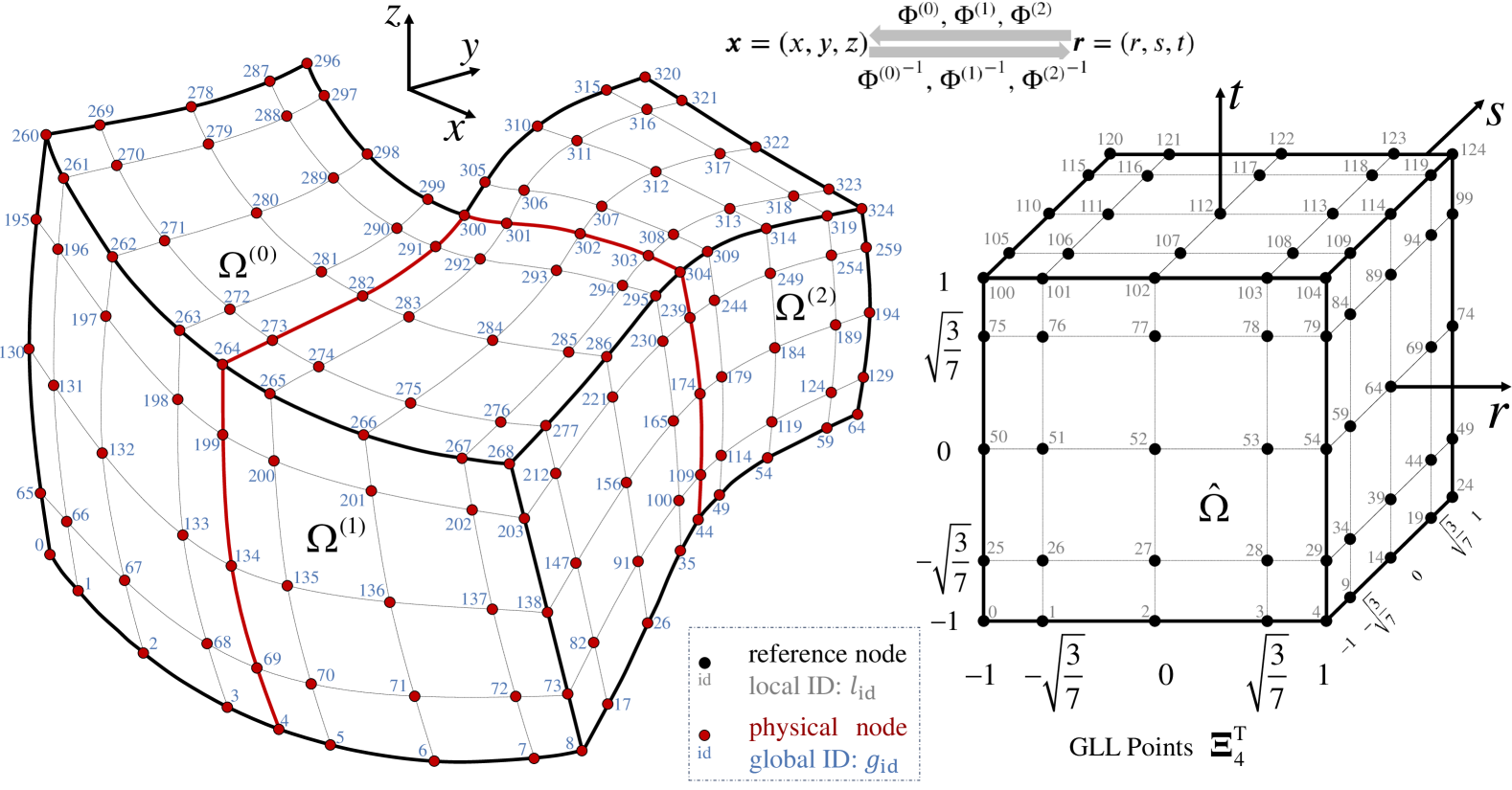
Figure 1. HOSFEM discretization example: $(E,N,\mathcal{N})$=(3,4,325).

2.2. Matrix-Free HOSFEM Kernels

For simplicity, we define $N_{1}=N+1$. Taking the Helmholtz/Poisson equation as an example, we introduce the fundamental principles of the matrix-free method. The Helmholtz equation is defined as:

(1) $$-\nabla\cdot(\lambda_{0}(\bm{x})\nabla\bm{u}(\bm{x}))+\lambda_{1}(\bm{x})\bm{u}(\bm{x})=\bm{f}(\bm{x}),\quad\bm{x}\in\Omega\subset\mathbb{R}^{3},$$

where: 1) $\bm{u}$ is the unknown scalar ($d=1$) or vector ($d=3$) field. 2) $\bm{f}$ is the source term. 3) $\lambda_{0}(\bm{x})$ and $\lambda_{1}(\bm{x})$ are given scalar fields. It reduces to the Poisson equation when $\lambda_{0}(\bm{x})\equiv 1$ and $\lambda_{1}(\bm{x})\equiv 0$. After HOSFEM discretization, the linear system is $\mathbf{A}\mathbf{u}=\mathbf{b}$, where

(2) $$\mathbf{A}=\mathbf{Q}^{\mathrm{T}}\begin{bmatrix}\mathbf{A}^{(0)}&&&\\ &\mathbf{A}^{(1)}&&\\ &&\ddots&\\ &&&\mathbf{A}^{(E-1)}\end{bmatrix}\mathbf{Q}.$$

Here, for each element $e$, the local $N_{1}^{3}\times N_{1}^{3}$ matrix is given by:

(3) $$\mathbf{A}^{(e)}=\mathbf{D}^{\mathrm{T}}\begin{bmatrix}\mathbf{\Lambda}_{0}^{(e)}&&\\ &\mathbf{\Lambda}_{0}^{(e)}&\\ &&\mathbf{\Lambda}_{0}^{(e)}\end{bmatrix}\begin{bmatrix}\mathbf{G}_{00}^{(e)}&\mathbf{G}_{01}^{(e)}&\mathbf{G}_{02}^{(e)}\\ \mathbf{G}_{01}^{(e)}&\mathbf{G}_{11}^{(e)}&\mathbf{G}_{12}^{(e)}\\ \mathbf{G}_{02}^{(e)}&\mathbf{G}_{12}^{(e)}&\mathbf{G}_{22}^{(e)}\end{bmatrix}\mathbf{D}+\mathbf{\Lambda}_{1}^{(e)}\mathbf{G}_{\mathrm{wj}}^{(e)},$$

where:

• $\mathbf{\Lambda}_{0}^{(e)}$ and $\mathbf{\Lambda}_{1}^{(e)}$ are diagonal matrices of size $N_{1}^{3}\times N_{1}^{3}$, with their diagonal elements representing the values of $\lambda_{0}(\bm{x})$ and $\lambda_{1}(\bm{x})$ at each node in element $e$.

• All geometric factors of element $e$ form 7 diagonal matrices of size $N_{1}^{3}\times N_{1}^{3}$: $\mathbf{G}_{00}^{(e)}$, $\mathbf{G}_{01}^{(e)}$, $\mathbf{G}_{02}^{(e)}$, $\mathbf{G}_{11}^{(e)}$, $\mathbf{G}_{12}^{(e)}$, $\mathbf{G}_{22}^{(e)}$, $\mathbf{G}_{\mathrm{wj}}^{(e)}$.

• $\mathbf{D}$ is the discrete form of the gradient $\nabla$, defined as

  (4) $$\mathbf{D}:=\begin{bmatrix}\mathbf{D}_{r}\\ \mathbf{D}_{s}\\ \mathbf{D}_{t}\end{bmatrix}:=\begin{bmatrix}\mathbf{I}\otimes\mathbf{I}\otimes\hat{\mathbf{D}}_{N}\\ \mathbf{I}\otimes\hat{\mathbf{D}}_{N}\otimes\mathbf{I}\\ \hat{\mathbf{D}}_{N}\otimes\mathbf{I}\otimes\mathbf{I}\end{bmatrix},$$

  where $\mathbf{I}$ is the identity matrix of size $N_{1}\times N_{1}$ and $\otimes$ denotes the tensor-product operation. $\mathbf{D}$ has size $3N_{1}^{3}\times N_{1}^{3}$.

$\mathbf{A}$ is of size $\mathcal{N}\times\mathcal{N}$. Matrix-based methods, such as those used in HPCG, store $\mathbf{A}$ in a sparse format and compute $\mathbf{Y}=\mathbf{A}\mathbf{X}$ through sparse matrix-vector multiplication (SpMV). In contrast, HOSFEM does not store $\mathbf{A}$ or even $\mathbf{A}^{(e)}$, but rather utilizes Algorithm 1. Although the gather-scatter kernel performs the multiplication of $\mathbf{Q}$ (or $\mathbf{Q}^{\mathrm{T}}$) and the vector, in practice, $\mathbf{Q}$ and $\mathbf{Q}^{\mathrm{T}}$ are never explicitly constructed. Instead, their actions are implemented within the communication library gslib.

Input : $\mathbf{\Lambda}_{0}^{(e)}$, $\mathbf{\Lambda}_{1}^{(e)}$, $\mathbf{G}_{00}^{(e)}$, …, $\mathbf{G}_{22}^{(e)}$, $\mathbf{G}_{\mathrm{wj}}^{(e)}$, $\hat{\mathbf{D}}_{N}$: sub-blocks in Eq. (3).       $\mathbf{X}$: $\mathcal{N}\times d$ matrix ($d$ vectors).             $\mathbf{Q}$: global-to-local matrix.

Output : $\mathbf{Y}$: $\mathcal{N}\times d$ matrix.

$\{\mathbf{X}^{(e)}\}\leftarrow\mathrm{scatter}(\mathbf{Q},\mathbf{X})$;

  // global-to-local, $\mathbf{X}^{(e)}$: $N_{1}^{3}\times d$

// $\{\mathbf{X}^{(e)}\}$: shorthand for set $\{\mathbf{X}^{(e)}|0\leq e<E\}$

1 $\{\mathbf{Y}^{(e)}\}\leftarrow\mathrm{axhelm}(\{\mathbf{\Lambda}_{0}^{(e)},\mathbf{\Lambda}_{1}^{(e)},\mathbf{G}_{00}^{(e)},...,\mathbf{G}_{22}^{(e)},\mathbf{G}_{\mathrm{wj}}^{(e)},\mathbf{X}^{(e)}\},\hat{\mathbf{D}}_{N})$;

$\mathbf{Y}\leftarrow\mathrm{gather}(\mathbf{Q}^{\mathrm{T}},\{\mathbf{Y}^{(e)}\})$;

  // local-to-global, $\mathbf{Y}^{(e)}$: $N_{1}^{3}\times d$

Algorithm 1 Matrix-free method for $\mathbf{Y}=\mathbf{A}\mathbf{X}$

Figure 2. PCG framework of Nekbone.

Nekbone uses the PCG method (Figure 2) in double precision to solve the Poisson/Helmholtz equation for scalar/vector fields within a box-shaped domain. The domain is divided into $E=n_{x}\times n_{y}\times n_{z}$ equally sized box elements. As a proxy application, Nekbone employs either simple preconditioning (JACOBI) or no preconditioning (COPY). This setup restricts computation to the axhelm kernel (Table 2) and communication to the gather-scatter kernel (Markidis et al., 2015; Ivanov et al., 2015; Gong et al., 2016; Chalmers et al., 2023), making Nekbone a minimal yet representative framework for studying the two most critical matrix-free kernels in HOSFEM.

Table 2. Time proportion and ranking of axhelm kernels in related works on Nekbone.

Ranking Proportion Platform 1 or 2 25.83-86.73% AMD EPYC 7763 (Chen et al., 2025), Intel Xeon Gold 6132 (Chen et al., 2025) core - K20X GPU (Gong et al., 2016), M2090 GPU (Gong et al., 2016), A64FX (Tsuji et al., 2022) 1 - Intel Xeon E5-2698v3 (Beskow) (Ivanov et al., 2015) 1 - P100 GPU (Karp et al., 2020), V100 GPU (Karp et al., 2020) 1 75% A64FX (Jackson et al., 2020), Alveo U280 FPGA (Brown, 2020) 1 81.8% K20X GPU (Titan) (Markidis et al., 2015)

2.3. Axhelm: Core Computation in HOSFEM

Definition 0 (Tensor Contraction).

Let $\mathbf{x}$ be an $N_{1}^{3}$ vector. Let $\mathbf{y}_{r}=\mathbf{D}_{r}\mathbf{x}$, $\mathbf{y}_{s}=\mathbf{D}_{s}\mathbf{x}$, and $\mathbf{y}_{t}=\mathbf{D}_{t}\mathbf{x}$ ($\mathbf{D}_{r}^{\mathrm{T}}$, $\mathbf{D}_{s}^{\mathrm{T}}$, and $\mathbf{D}_{t}^{\mathrm{T}}$ are similar). Then, $\mathbf{y}_{r}$, $\mathbf{y}_{s}$, and $\mathbf{y}_{t}$ can be computed as follows for $0\leq i,j,k\leq N$:

(5) $$\begin{matrix}\mathbf{y}_{r}(i,j,k)=\sum_{0\leq m\leq N}\hat{\mathbf{D}}_{N}(i,m)\mathbf{x}(m,j,k),\\ \mathbf{y}_{s}(i,j,k)=\sum_{0\leq m\leq N}\hat{\mathbf{D}}_{N}(j,m)\mathbf{x}(i,m,k),\\ \mathbf{y}_{t}(i,j,k)=\sum_{0\leq m\leq N}\hat{\mathbf{D}}_{N}(k,m)\mathbf{x}(i,j,m),\end{matrix}$$

where the 3D index $(i,j,k)$ represents the $i+jN_{1}+kN_{1}^{2}$-th row.

The kernel used to compute $\mathbf{Y}^{(e)}=\mathbf{A}^{(e)}\mathbf{X}^{(e)}$ has various names, such as Ax (Min et al., 2024; Karp et al., 2021), AX (Brown, 2020),or ax3D (Markidis et al., 2015). This paper adopts the name axhelm (Tsuji et al., 2022; Nek5000 Team, 2025). As an example, consider the case when $d=1$ (scalar field: $\mathbf{X}^{(e)}$ has only one column). One of the state-of-the-art implementations of axhelm from Nekbone/RS is presented in Algorithm 2. It employs the 2D thread block structure (Świrydowicz et al., 2019): 1) Each block processes for a single element $e$. 2) Each block employs a layer of $N_{1}\times N_{1}$ threads to process $N_{1}$ k-layers in lock-step.

The primary computational workload (Lines 15-16, 24-25) arises from six tensor contractions (Definition 1), each involving the multiplication of a tensor-product (e.g., $\mathbf{D}_{r}$) with a vector, requiring $2N_{1}^{4}$ FLOPs. Tensor contraction arises from the sum factorization technique (M. O. Deville et al., 2003; Fischer et al., 2022; Min et al., 2024), which exploits the local tensor-product structure to reduce the computational complexity of $\mathbf{Y}^{(e)}=\mathbf{A}^{(e)}\mathbf{X}^{(e)}$ from $\mathcal{O}(N_{1}^{6})$ to $\mathcal{O}(N_{1}^{4})$. This is the fundamental source of HOSFEM’s high performance. In addition, Lines 17-21 incorporate the geometric and scalar factors. For Poisson equation ($\lambda_{0}=1$ and $\lambda_{1}=0$), Line 10, 21 and ”$\lambda_{0}*$” in Lines 17-19 are unnecessary.

Input : $\mathbf{\Lambda}_{0}^{(e)},\mathbf{\Lambda}_{1}^{(e)},\mathbf{G}_{00}^{(e)},...,\mathbf{G}_{22}^{(e)},\mathbf{G}_{\mathrm{wj}}^{(e)},\mathbf{X}^{(e)},\hat{\mathbf{D}}_{N}$.

Output : $\mathbf{Y}^{(e)}$ (both input and output are in global memory).

1 e = blockIdx.x; j = threadIdx.y; i = threadIdx.x;

s_Dhat[j][i] = $\hat{\mathbf{D}}_{N}$(j,i);

  // ’s_’ means shared memory

2 for $0\leq\mathrm{k}\leq N$ do

3    x[k] = $\mathbf{X}^{(e)}$(i,j,k); y[k] = 0;

4   

5syncthreads();

6 for $0\leq\mathrm{k}\leq N$ do

    g00 = $\mathbf{G}_{00}^{(e)}$(i,j,k); g01 = $\mathbf{G}_{01}^{(e)}$(i,j,k); g02 = $\mathbf{G}_{02}^{(e)}$(i,j,k);

     // only

    g11 = $\mathbf{G}_{11}^{(e)}$(i,j,k); g12 = $\mathbf{G}_{12}^{(e)}$(i,j,k); g22 = $\mathbf{G}_{22}^{(e)}$(i,j,k);

     // access

7    if $\mathrm{isHelm}$ then

       gwj = $\mathbf{G}_{\mathrm{wj}}^{(e)}$(i,j,k); $\lambda_{0}$ = $\mathbf{\Lambda}_{0}^{(e)}$(i,j,k); $\lambda_{1}$ = $\mathbf{\Lambda}_{1}^{(e)}$(i,j,k);

        // diag.

8      

9   s_x[j][i] = x[k];

10    syncthreads();

11    xr = 0; xs = 0; xt = 0; tmp = 0;

12    for $0\leq\mathrm{m}\leq N$ do

       xr+=s_Dhat[i][m]*s_x[j][m];

        // $\mathbf{D}_{r},\mathbf{D}_{s},\mathbf{D}_{t}$

13       xs+=s_Dhat[j][m]*s_x[m][i]; xt+=s_Dhat[k][m]*x[m];

14      

15   s_gxr[j][i] = $\lambda_{0}$ * (g00 * xr + g01 * xs + g02 * xt);

16    s_gxs[j][i] = $\lambda_{0}$ * (g01 * xr + g11 * xs + g12 * xt);

17    gxt    = $\lambda_{0}$ * (g02 * xr + g12 * xs + g22 * xt);

18    if $\mathrm{isHelm}$ then

       tmp = gwj * $\lambda_{1}$ * x[k];

        // isHelm: Helmholtz/Poisson

19      

20   syncthreads();

21    for $0\leq\mathrm{m}\leq N$ do

       tmp+=s_Dhat[m][i]*s_gxr[j][m];

        // $\mathbf{D}_{r}^{\mathrm{T}},\mathbf{D}_{s}^{\mathrm{T}},\mathbf{D}_{t}^{\mathrm{T}}$

22       tmp+=s_Dhat[m][j]*s_gxs[m][i];  y[m]+=s_Dhat[k][m]*gxt;

23      

24   y[k] += tmp;

25   

26for $0\leq\mathrm{k}\leq N$ do

27    $\mathbf{Y}^{(e)}$(i,j,k) = y[k];

28   

Algorithm 2 Original axhelm kernel for a scalar field

3. The Proposed Method

3.1. Bottleneck Analysis of Axhelm

Different studies suggest varying appropriate ranges for $N$: $7\leq N\leq 11$ (Karp et al., 2022b), $N\leq 10$ (NekRS Team, 2025), and $7\leq N\leq 15$ (Table 2). Although some studies investigate smaller values (Fischer et al., 2020), the most commonly used $N$ is 7 (Fischer et al., 2022; Jansson et al., 2023; Karp et al., 2022a; Jansson et al., 2024; Min et al., 2025; Karp et al., 2022b; Tsuji et al., 2022). For a single element, the computation of the axhelm requires: 1) $12N_{1}^{4}$ FLOPs for six tensor contractions. 2) $15N_{1}^{3}$ FLOPs for geometric factors. 3) Additional $5N_{1}^{3}$ FLOPs for the scale factors in the Helmholtz equation. The above computational cost needs to be multiplied by $d$. Apart from the differentiation matrix, the total global memory access consists of two main parts:

(6) $$\text{geometric factors}: \ \ \mathcal{M}_{\text{geo}}=(6+\text{isHelm})N_{1}^{3}\times\text{FPSize},$$

(7) $$\mathbf{X}^{(e)}\mathbf{Y}^{(e)}\mathbf{\Lambda}_{0}^{(e)}\mathbf{\Lambda}_{1}^{(e)}: \ \ \mathcal{M}_{\text{XYL}}=(2\times\text{isHelm}+2d)N_{1}^{3}\times\text{FPSize}.$$

Here, isHelm is a binary value (0 or 1), indicating whether the Helmholtz equation is being solved, and FPSize refers to the size of the floating-point data type. The above statistics are summarized in Table 3. The operational intensity is defined as $\mathcal{I}=\mathcal{F}/\mathcal{M}$.

Table 3. Computational workload and memory access requirements for the original axhelm kernels.

Kernel Type	$\mathcal{F}_{\mathrm{ax}}$ (FLOP)	$\mathcal{M}_{\mathrm{orig}}$ (Byte)
Poisson, $d=1$	$12N_{1}^{4}+15N_{1}^{3}$	$(8N_{1}^{3}+N_{1}^{2})\times\text{FPSize}$
Helmholtz, $d=1$	$12N_{1}^{4}+20N_{1}^{3}$	$(11N_{1}^{3}+N_{1}^{2})\times\text{FPSize}$
Poisson, $d=3$	$36N_{1}^{4}+45N_{1}^{3}$	$(12N_{1}^{3}+N_{1}^{2})\times\text{FPSize}$
Helmholtz, $d=3$	$36N_{1}^{4}+60N_{1}^{3}$	$(15N_{1}^{3}+N_{1}^{2})\times\text{FPSize}$

The platform’s peak-to-bandwidth ratio is defined as $\text{PBR}=\frac{\mathcal{P}_{\text{peak}}}{\mathcal{B}}$, where $\mathcal{P}_{\text{peak}}$ is the theoretical peak performance and $\mathcal{B}$ is the maximum achievable global memory bandwidth. PBR is the minimum operational intensity required to achieve $\mathcal{P}_{\text{peak}}$ (Williams et al., 2009).

Figure 3 shows that at $N_{1}=18$, the operational intensity of the axhelm kernel (Poisson, $d=3$) exceeds one of the PBR lines. The following observations can be made: 1) The operational intensity shows a linear growth trend as $N$ increases. 2) The axhelm’s performance is constrained by memory bandwidth in real-world applications. Therefore, previous studies on the axhelm performance optimization have typically utilized a performance model (Świrydowicz et al., 2019; Karp et al., 2020) based on memory access bandwidth limitations:

(8) $$\mathcal{R}_{\text{orig}}=\mathcal{B}\cdot\frac{\mathcal{F}_{\text{ax}}}{\mathcal{M}_{\text{orig}}}.$$

Under this model, related work has seemingly approached their respective theoretical performance limits. This implies that continuing to optimize tensor contractions is no longer effective. To achieve further optimization, memory access must be reduced. Meanwhile, we note that the geometric factors account for a significant portion of memory access, but contribute only lower-order terms ($\mathcal{O}(N_{1}^{3})$) to the computational workload. So far, this paper, like most studies of the axhelm, treats the geometric factors as abstract constants. Next, we will clearly outline their computation process.

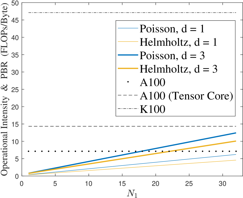
Figure 3. Operational intensity of the four axhelm kernels vs. PBR of the target platforms (FP64 precision, FPSize = 8).

3.2. Computation of Geometric Factors

The geometric factors are related to the Jacobian matrix. For each element $e$, the mapping $\Phi^{(e)}:\hat{\Omega}\to\Omega^{(e)}$, $(r,s,t)\mapsto(x,y,z)$, uniquely determines the Jacobian matrix function:

(9) $$\mathbf{J}^{\Phi^{(e)}}(r,s,t):=\begin{bmatrix}\frac{\partial{\Phi^{(e)}}(r,s,t)}{\partial r}\\ \frac{\partial{\Phi^{(e)}}(r,s,t)}{\partial s}\\ \frac{\partial{\Phi^{(e)}}(r,s,t)}{\partial t}\end{bmatrix}^{\mathrm{T}}=\begin{bmatrix}\frac{\partial x}{\partial r}&\frac{\partial x}{\partial s}&\frac{\partial x}{\partial t}\\ \frac{\partial y}{\partial r}&\frac{\partial y}{\partial s}&\frac{\partial y}{\partial t}\\ \frac{\partial z}{\partial r}&\frac{\partial z}{\partial s}&\frac{\partial z}{\partial t}\end{bmatrix}$$

This defines a $3\times 3$ matrix at any point $(r,s,t)\in\hat{\Omega}=[-1,1]^{3}$. Therefore, at each physical node $(e,i,j,k)$, there is a corresponding, unique Jacobian matrix of size $3\times 3$:

(10) $$\mathbf{J}_{ijk}^{(e)}:=\mathbf{J}^{\Phi^{(e)}}(\xi_{i},\xi_{j},\xi_{k}).$$

The 7 geometric factors at the physical node are then defined as:

(11) $$w_{i}w_{j}w_{k}|\mathbf{J}_{ijk}^{(e)}|\cdot{\mathbf{J}_{ijk}^{(e)}}^{-1}{\mathbf{J}_{ijk}^{(e)}}^{\mathrm{-T}}\quad\text{and}\quad w_{i}w_{j}w_{k}|\mathbf{J}_{ijk}^{(e)}|,$$

where the latter is a scalar, and the former is a $3\times 3$ symmetric matrix (with only 6 values needed). The computational cost of obtaining the geometric factors from the Jacobian matrix is easily estimated, primarily involving the calculation of a $3\times 3$ determinant and the inverse of a $3\times 3$ matrix.

The problem ”How to cost-effectively obtain the geometric factors” can be reformulated as ”How to cost-effectively obtain the Jacobian matrix.” However, for a general $\Phi^{(e)}$ without an analytical expression, we can only obtain the Jacobian matrix through the following discrete and transposed form of Equation (9):

(12) $$\mathbf{D}\mathbf{C}_{\text{nodes}}^{(e)} =\begin{bmatrix}\mathbf{D}_{r}\mathbf{C}_{\text{nodes}}^{(e)}\\ \mathbf{D}_{s}\mathbf{C}_{\text{nodes}}^{(e)}\\ \mathbf{D}_{t}\mathbf{C}_{\text{nodes}}^{(e)}\end{bmatrix}=\begin{bmatrix}\mathbf{D}_{r}\mathbf{x}_{\text{nodes}}^{(e)}&\mathbf{D}_{r}\mathbf{y}_{\text{nodes}}^{(e)}&\mathbf{D}_{r}\mathbf{z}_{\text{nodes}}^{(e)}\\ \mathbf{D}_{s}\mathbf{x}_{\text{nodes}}^{(e)}&\mathbf{D}_{s}\mathbf{y}_{\text{nodes}}^{(e)}&\mathbf{D}_{s}\mathbf{z}_{\text{nodes}}^{(e)}\\ \mathbf{D}_{t}\mathbf{x}_{\text{nodes}}^{(e)}&\mathbf{D}_{t}\mathbf{y}_{\text{nodes}}^{(e)}&\mathbf{D}_{t}\mathbf{z}_{\text{nodes}}^{(e)}\\ \end{bmatrix}$$

Here, $\mathbf{C}_{\text{nodes}}^{(e)}=[\mathbf{x}_{\text{nodes}}^{(e)},\mathbf{y}_{\text{nodes}}^{(e)},\mathbf{z}_{\text{nodes}}^{(e)}]$ is the $N_{1}^{3}\times 3$ matrix of physical node coordinates in element $e$, which is naturally the discrete form of $\Phi^{(e)}$ as a sampled subset. $\mathbf{D}_{r}$, $\mathbf{D}_{s}$, and $\mathbf{D}_{t}$ represent the discrete forms of the partial differential operators $\frac{\partial}{\partial r}$, $\frac{\partial}{\partial s}$, and $\frac{\partial}{\partial t}$, respectively. The final result is a $3N_{1}^{3}\times 3$ matrix representing the $3\times 3$ Jacobian matrix of the $N_{1}^{3}$ nodes in element $e$.

Continuous: $$\Phi^{(e)} \xrightarrow{\text{Eq. }\eqref{Jacobian_matrix_function}} \mathbf{J}^{\Phi^{(e)}}$$

$$\downarrow \text{Eq. }\eqref{Jacobian_matrix_at_node}$$

Discrete: $$\mathbf{C}_{\text{nodes}}^{(e)} \xrightarrow{\text{Eq. }\eqref{Jacobian_matrix_tensor_contraction}} \mathbf{J}_{ijk}^{(e)} \xrightarrow{\text{Eq. }\eqref{Jacobian_matrix_to_geometric_factors}}\begin{array}[]{c}\text{Geometric}\\ \text{Factors}\end{array}$$

The above figure summarizes both the continuous and discrete representations of the Jacobian matrix. The discrete approach applies to any deformed hexahedral element. However, for a single hexahedral element, this method involves $3N_{1}^{3}$ memory references to node coordinates, 9 tensor contractions (totaling $18N_{1}^{4}$ FLOPs), and $N_{1}^{3}$ evaluations of Equation (11). Introducing this overhead into the axhelm kernel to replace $6N_{1}^{3}$ or $7N_{1}^{3}$ memory references for geometric factors is not worthwhile. However, when $\Phi^{(e)}$ has a simple analytical expression, $\mathbf{J}^{\Phi^{(e)}}$ often does as well. In this case, the continuous approach (Equation (10)) can efficiently compute the Jacobian matrices at each physical node.

The continuous (analytical) approach does not apply to all elements. Therefore, it must be designed for a specific type of hexahedral element: 1) It is sufficiently simple to ensure an analytical expression for its Jacobian matrix. 2) It is flexible enough to be widely applicable across various meshes. In Section 3.3, we see that the trilinear element is a suitable candidate for this purpose.

3.3. Low-Cost Recalculation of Geometric Factors for Trilinear Elements

Definition 0 (Trilinear Element).

Given eight vertices coordinates $\mathbf{v}_{i}\in\mathbb{R}^{3}$, $0\leq i\leq 7$, a trilinear element is uniquely determined by the mapping $(x,y,z)=\Phi(r,s,t):=\sum_{i=0}^{7}\sigma_{i}(r,s,t)\mathbf{v}_{i},$ where $(r,s,t)\in\hat{\Omega}=[-1,1]^{3}$ and the functions $\sigma_{i}$ are defined as
$\sigma_{0}(r,s,t)=\frac{1}{8}(1-r)(1-s)(1-t),\sigma_{1}(r,s,t)=\frac{1}{8}(1+r)(1-s)(1-t),\\ \sigma_{2}(r,s,t)=\frac{1}{8}(1-r)(1+s)(1-t),\sigma_{3}(r,s,t)=\frac{1}{8}(1+r)(1+s)(1-t),\\ \sigma_{4}(r,s,t)=\frac{1}{8}(1-r)(1-s)(1+t),\sigma_{5}(r,s,t)=\frac{1}{8}(1+r)(1-s)(1+t),\\ \sigma_{6}(r,s,t)=\frac{1}{8}(1-r)(1+s)(1+t),\sigma_{7}(r,s,t)=\frac{1}{8}(1+r)(1+s)(1+t).$

As a fundamental Q1 type (with linear shape functions) in both geometric modeling and FEM, the trilinear element has long been favored by researcher (Cifuentes and Kalbag, 1992; Ilic and Notaros, 2001; Korelc and Wriggers, 1996; Ilic and Notaros, 2003; Simo et al., 1993; Schneider et al., 2019). As shown in Figure 4 and Definition 1, a trilinear element is uniquely determined by eight freely chosen vertices(M. O. Deville et al., 2003). The flexibility allows for the arbitrary selection of vertices, which in turn determines the edges, faces, and the whole element. This enables the trilinear element to adapt to complex geometries and effectively fill the global domain $\Omega$. It is a feasible and common practice to fill $\Omega$ entirely using trilinear elements. If higher precision is needed, more sophisticated higher-order elements, such as Q2 or Q3 (Schneider et al., 2019), are typically employed only at the boundaries of $\Omega$. Based on our statistics of the mesh (Figure 5) used in a typical NekRS application (Fischer et al., 2022; Team, 2025c), boundary elements account for only 11%. This indicates that trilinear elements possess sufficient versatility and a high proportion of the overall mesh. Moreover, the trilinear element has an analytical Jacobian matrix.

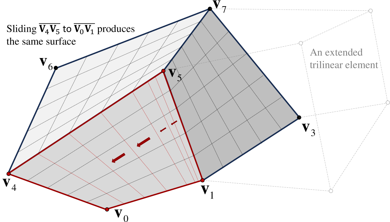
Figure 4. A trilinear element: 1) Each edge is a line segment. 2) The line segment $\overline{\mathbf{v}_{1}\mathbf{v}_{5}}$ slides to $\overline{\mathbf{v}_{0}\mathbf{v}_{4}}$, forming a ruled surface, with similar surfaces for the other faces. By placing vertices around it, more trilinear elements can be expanded.

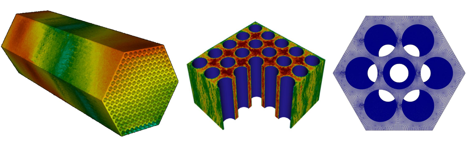
Figure 5. A mesh: nuclear fuel rod cooling fluid simulation.

Let $\mathbf{V}^{(e)}=(\mathbf{v}_{0}^{\mathrm{T}},...,\mathbf{v}_{7}^{\mathrm{T}})^{\mathrm{T}}$ is a matrix of size $8\times 3$. It is also noted that the trilinear mapping has a compact tensor-product form:

(13) $$\Phi^{(e)}(r,s,t)=\frac{1}{8}[(1-t,1+t)\otimes(1-s,1+s)\otimes(1-r,1+r)]\mathbf{V}^{(e)}.$$

Substituting Equation (13) into Equation (9), we obtain

(14) $$\mathbf{J}^{\Phi^{(e)}}(r,s,t)=\frac{1}{8}{\mathbf{V}^{(e)}}^{\mathrm{T}}\begin{bmatrix}(1-t,1+t)\otimes(1-s,1+s)\otimes(-1,1)\\ (1-t,1+t)\otimes(-1,1)\otimes(1-r,1+r)\\ (-1,1)\otimes(1-s,1+s)\otimes(1-r,1+r)\end{bmatrix}^{\mathrm{T}}.$$

However, directly substituting $\mathbf{J}^{\Phi^{(e)}}(\xi_{i},\xi_{j},\xi_{k})$ ($0\leq i,j,k\leq N$) into Equation (14) and expanding it to compute $\mathbf{J}_{ijk}^{(e)}$ remains impractical. Because even a single node requires a $3\times 3\times 8$ matrix multiplication, the computational cost (144 FLOPs) remains high. To enhance efficiency, we must analyze the formula’s structure, identify common terms, and extract invariant components for optimization. Based on this, we propose Algorithm 3, with key design aspects as follows:

Input : $\mathbf{V}^{(e)}$: stored in s_V[8][3].

1 e = blockIdx.x; j = threadIdx.y; i = threadIdx.x;

2 s = c_gllx[j]; r = c_gllx[i]; tmp[3] = {0, 0, 0};

3 s0 = 1 - s; s1 = 1 + s; r0 = 1 - r; r1 = 1 + r;

4 if $j<3$ then

5    tmp1 = r0 * (s_V[1][j] - s_V[0][j]) + r1 * (s_V[3][j] - s_V[2][j]);

6    tmp2 = r0 * (s_V[5][j] - s_V[4][j]) + r1 * (s_V[7][j] - s_V[6][j]);

7    tmp3 = r0 * (s_V[2][j] - s_V[0][j]) + r1 * (s_V[3][j] - s_V[1][j]);

8    tmp4 = r0 * (s_V[6][j] - s_V[4][j]) + r1 * (s_V[7][j] - s_V[5][j]);

9    s_E0[i][j] = tmp1 + tmp2; s_E1[i][j] = tmp2 - tmp1;

10    s_F0[i][j] = tmp3 + tmp4; s_F1[i][j] = tmp4 - tmp3;

11   

12for $0\leq\mathrm{d}<3$ do

13    tmp[d]=r0*s0*(s_V[4][d]-s_V[0][d])+r1*s0*(s_V[5][d]-s_V[1][d]) +r1*s1*(s_V[7][d]-s_V[3][d])+r0*s1*(s_V[6][d]-s_V[2][d]);

14   

15J02 = tmp[0]; J12 = tmp[1]; J22 = tmp[2];

gllw_ij_div_8 = 0.125 * c_gllw[i] * c_gllw[j];

  // constant $\mathbf{W}_{N}$

16 syncthreads();

17 for $0\leq\mathrm{k}\leq N$ do

    t = c_gllx[k];

     // ’c_’: constant memory copy of $\mathbf{\Xi}_{N}$

18    J00=s_E0[j][0]+t*s_E1[j][0]; J01=s_F0[i][0]+t*s_F1[i][0];

19    J10=s_E0[j][1]+t*s_E1[j][1]; J11=s_F0[i][1]+t*s_F1[i][1];

20    J20=s_E0[j][2]+t*s_E1[j][2]; J21=s_F0[i][2]+t*s_F1[i][2];

21   

22   JJ00=J00*J00+J10*J10+J20*J20; JJ01=J00*J01+J10*J11+J20*J21;

23    JJ02=J00*J02+J10*J12+J20*J22; JJ11=J01*J01+J11*J11+J21*J21;

24    JJ12=J01*J02+J11*J12+J21*J22; JJ22=J02*J02+J12*J12+J22*J22;

25   

26   detJ = J00 * (J11 * J22 - J21 * J12) - J10 * (J01 * J22 - J21 * J02)    + J20 * (J01 * J12 - J11 * J02);

27    gScale = gllw_ij_div_8 * c_gllw[k] / detJ;

28    g00=(JJ11*JJ22-JJ12*JJ12)*gScale; g01=(JJ02*JJ12-JJ01*JJ22)*gScale;

29    g02=(JJ01*JJ12-JJ02*JJ11)*gScale; g11=(JJ00*JJ22-JJ02*JJ02)*gScale;

30    g12=(JJ01*JJ02-JJ00*JJ12)*gScale; g22=(JJ00*JJ11-JJ01*JJ01)*gScale;

31    if $\mathrm{isHelm}$ then

32       gwj = gScale * detJ * detJ * 0.015625;

33      

34   

Algorithm 3 Geometric factors Recalculation (trilinear)

1) Invariant Components (Lines 11-13): Each thread $(i,j)$ needs to compute $N_{1}$ matrices of $\mathbf{J}_{ijk}^{(e)}$ ($0\leq k\leq N$). It is important to note that the third column of $\mathbf{J}^{\Phi^{(e)}}(r,s,t)$ in Equation (14) depends only on $r$ and $s$, meaning the third column of $\mathbf{J}_{ijk}^{(e)}$ is only dependent on $i$ and $j$. Therefore, this column only needs to be computed once and can be shared across the $k$-loop.

2) Common Terms (Lines 4-10): Noting that the transpose of the first column of $\mathbf{J}_{ijk}^{(e)}$ is given by (the second column is analogous)

(15) $$\begin{matrix}&[(1-\xi_{k},1+\xi_{k})\otimes(1-\xi_{j},1+\xi_{j})\otimes(-1,1)]{\mathbf{V}^{(e)}}=\\ &\quad[(1,1)\otimes(1-\xi_{j},1+\xi_{j})\otimes(-1,1)]{\mathbf{V}^{(e)}}+\mathrel{\phantom{-\xi_{k}}}\\ &\quad[(-1,1)\otimes(1-\xi_{j},1+\xi_{j})\otimes(-1,1)]{\mathbf{V}^{(e)}}\cdot\xi_{k}.\end{matrix}$$

Here, Except for $\xi_{k}$, the remaining parts are shared among threads $(i,j)$ with the same $j$. Therefore, we can precompute four matrices, $\mathbf{E}_{0}$, $\mathbf{E}_{1}$, $\mathbf{F}_{0}$, and $\mathbf{F}_{1}$, each of size $N_{1}\times 3$, before the $k$-loop and store them in shared memory to eliminate redundant computations:

(16) $$\begin{matrix}&\mathbf{E}_{0}=\mathrel{\phantom{-}}[(1,1)\otimes(\mathbf{1}-\mathbf{\Xi}_{N},\mathbf{1}+\mathbf{\Xi}_{N})\otimes(-1,1)]\mathbf{V}^{(e)},\\ &\mathbf{E}_{1}=[(-1,1)\otimes(\mathbf{1}-\mathbf{\Xi}_{N},\mathbf{1}+\mathbf{\Xi}_{N})\otimes(-1,1)]\mathbf{V}^{(e)},\\ &\mathbf{F}_{0}=\mathrel{\phantom{-}}[(1,1)\otimes(-1,1)\otimes(\mathbf{1}-\mathbf{\Xi}_{N},\mathbf{1}+\mathbf{\Xi}_{N})]\mathbf{V}^{(e)},\\ &\mathbf{F}_{1}=[(-1,1)\otimes(-1,1)\otimes(\mathbf{1}-\mathbf{\Xi}_{N},\mathbf{1}+\mathbf{\Xi}_{N})]\mathbf{V}^{(e)},\\ \end{matrix}$$

where $\mathbf{1}$ is an $N_{1}$-dimensional column vector of ones. Thanks to the common terms, the six values in the first and second columns of $\mathbf{J}_{ijk}^{(e)}$ can be recomputed with only 12 FLOPs (Lines 18-20).

3) Jacobian Matrix to Geometric Factors (Lines 21-30): After obtaining the Jacobian matrix $\mathbf{J}_{ijk}^{(e)}$ of a node, for the computation in Equation (11), we first compute $\mathbf{K}={\mathbf{J}_{ijk}^{(e)}}^{\mathrm{T}}\mathbf{J}_{ijk}^{(e)}$ and then

(17) $$|\mathbf{J}_{ijk}^{(e)}|\cdot{\mathbf{J}_{ijk}^{(e)}}^{-1}{\mathbf{J}_{ijk}^{(e)}}^{\mathrm{-T}}=|\mathbf{J}_{ijk}^{(e)}|\cdot\mathbf{K}^{-1}=|\mathbf{J}_{ijk}^{(e)}|\cdot\frac{\text{adj}(\mathbf{K})}{|\mathbf{K}|}=\frac{\text{adj}(\mathbf{K})}{|\mathbf{J}_{ijk}^{(e)}|},$$

where $\text{adj}(\mathbf{K})$ is the adjugate matrix of $\mathbf{K}$. Meanwhile, introduced by $\frac{1}{8}$ and the GLL weights, the scaling coefficient (gScale) is deferred to the final stage of the algorithm. In summary, Algorithm 3 replaces the memory references for the geometric factors with 24 memory references for $\mathbf{V}^{(e)}$ and $72N_{1}+51N_{1}^{2}+(82+\mathrm{isHelm}\times 3)N_{1}^{3}$ FLOPs.

For the special case of trilinear elements, parallelepipeds, Algorithm 4 enables geometric factor recomputation at virtually zero cost, since $\mathbf{J}^{\Phi^{(e)}}(r,s,t)\equiv\mathbf{J}^{(e)}$ remains constant. further, at each node $(e,i,j,k)$, $\mathbf{J}_{ijk}^{(e)}=\mathbf{J}^{(e)}$. Thus, in Equation (11), the geometric factors excluding GLL weights, i.e., $|\mathbf{J}^{(e)}|\cdot{\mathbf{J}^{(e)}}^{-1}{\mathbf{J}^{(e)}}^{\mathrm{-T}}$ and $|\mathbf{J}^{(e)}|$, can be get with just seven memory references. This property effectively removes the bottleneck associated with the geometric factors, making performance entirely dependent on tensor contractions.

Input : $h_{00}^{(e)},...,h_{22}^{(e)}$, and $h_{\mathrm{det}}^{(e)}$: geometric factors without GLL weights, stored in shared memory s_h[7].

1 e = blockIdx.x; j = threadIdx.y; i = threadIdx.x;

2 h00 = s_h[0]; h01 = s_h[1]; h02 = s_h[2];

3 h11 = s_h[3]; h12 = s_h[4]; h22 = s_h[5]; hdet= s_h[6];

4 gllw_ij = c_gllw[i] * c_gllw[j];

5 for $0\leq\mathrm{k}\leq N$ do

6    w = gllw_ij * c_gllw[k]; gwj = w * hdet;

7    g00 = w * h00; g01 = w * h01; g02 = w * h02;

8    g11 = w * h11; g12 = w * h12; g22 = w * h22;

9   

Algorithm 4 Geometric factors Recalculation (parallelepiped)

4. Implementation and optimization

4.1. Optimization of Geometric Factors

The optimization in this Section is discussed in terms of two types of equations, focusing on the trilinear element.

4.1.1. Merging Scalar Factors

For the Helmholtz equation, the axhelm kernel requires each node to access the scalar factors $\lambda_{0}$ and $\lambda_{1}$. It is important to note that: 1) In Algorithm 2, both $\lambda_{0}$ and $\lambda_{1}$ must be multiplied by the geometric factor. 2) In Algorithm 3, the recalculation of the geometric factor also involves a scaling coefficient, gScale (considered as a custom geometric factor). We can multiply gScale and gwj with $\lambda_{0}$ and $\lambda_{1}$, respectively:

$$\mathbf{\Lambda}_{2}^{(e)}=\mathbf{G}_{\mathrm{scale}}^{(e)}\mathbf{\Lambda}_{0}^{(e)},\qquad\text{and}\qquad\mathbf{\Lambda}_{3}^{(e)}=\mathbf{G}_{\mathrm{wj}}^{(e)}\mathbf{\Lambda}_{1}^{(e)}.$$

The computation of $\mathbf{\Lambda}_{2}^{(e)}$ and $\mathbf{\Lambda}_{3}^{(e)}$ will be completed before starting to solve the linear system, and they will be used as new scalar factors to be read by the axhelm kernel. This eliminates the computations related to gScale and gwj (Lines 24, 25, and 30) in Algorithm 3. Moreover, the costly division operations (Huang and Chen, 2015) are no longer needed.

4.1.2. Partial Recalculation

For the Poisson equation, the optimization in Section 4.1.1 is no longer effective because the axhelm in this case no longer involves $\mathbf{\Lambda}_{0}^{(e)}$, $\mathbf{\Lambda}_{1}^{(e)}$, and $\mathbf{G}_{\mathrm{wj}}^{(e)}$. However, we can revert the scaling coefficient gScale in Algorithm 3 to be obtained through memory access, instead of being recomputed in kernels (Lines 24-25). We refer to this approach as partial recomputation. This approach substitutes complex computation, including division, with memory accesses, making it a balanced solution.

Table 4 summarizes the overhead of various geometric factor acquisition approaches discussed in this paper and other existing methods, highlighting the flexibility in this process. Notably, our proposed approach exhibits significantly lower overhead compared to the others. In theory, numerous viable approaches exist, each corresponding to a distinct roofline model.

Table 4. Overhead of acquiring geometric factors for different approaches.

Approach General Parallelepiped Trilinear Existing Approaches Full Access Algorithm 4 Algorithm 3 Section 4.1 Remacle et al. (Remacle et al., 2016) NekRS (NekRS Team, 2025) Karp et al. (Karp et al., 2022b) $\mathcal{F}_{\mathrm{reGeo}}$ 0 $(7+\mathrm{isHelm})N_{1}^{3}$ $\begin{matrix}72N_{1}+51N_{1}^{2}\\ +(82+\mathrm{isHelm}\times 3)N_{1}^{3}\end{matrix}$ $72N_{1}+51N_{1}^{2}+66N_{1}^{3}$ $242N_{1}^{3}$ $296N_{1}^{3}$ $81N_{1}^{3}+18N_{1}^{4}$ $\mathcal{M}_{\mathrm{geo}}/\mathrm{FPSize}$ $(6+\mathrm{isHelm})N_{1}^{3}$ $6+\mathrm{isHelm}$ 24 $24+\mathrm{isPois}\times N_{1}^{3}$ 24 24 $24+N_{1}^{3}$

4.2. Optimization of Tensor Contractions

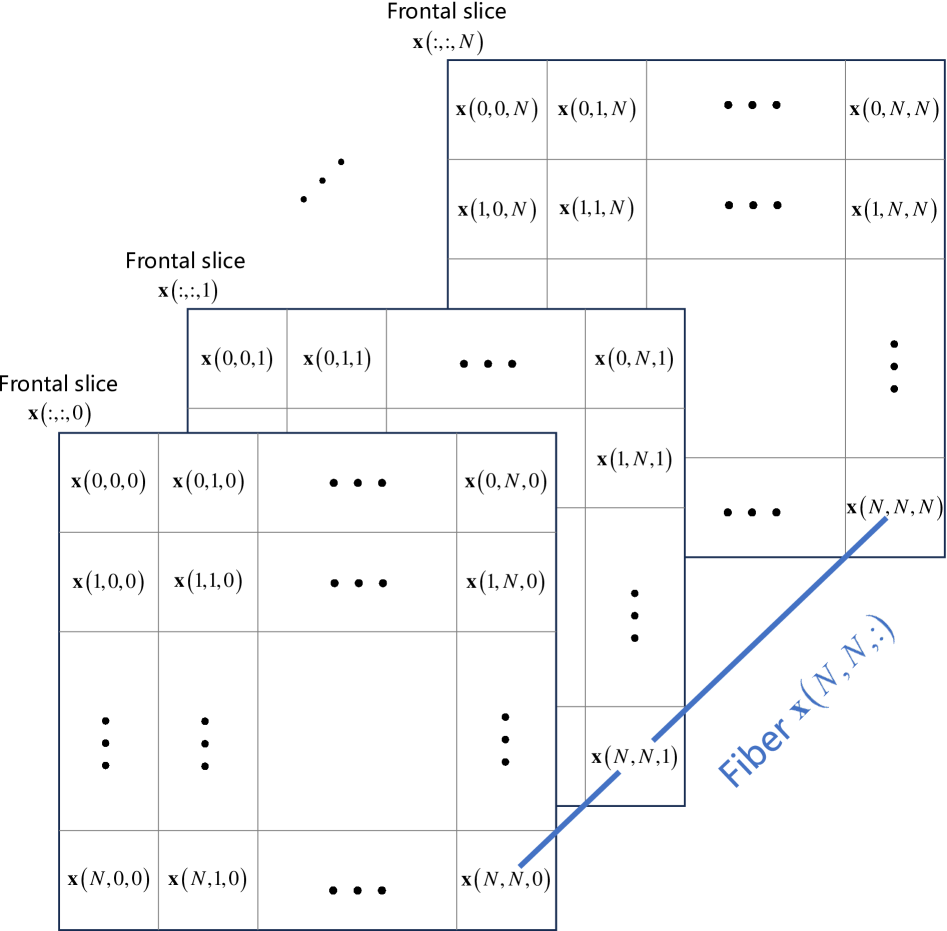
Figure 6. A third-order tensor, its slices, and fibers.

The majority of the computations in axhelm result from tensor contractions (Section 3.1). With the alleviation of the memory access bottleneck for geometric factors, tensor contraction now becomes the most time-critical operation to be accelerated.

As shown in Equation (5), a vector of size $N_{1}^{3}$ can be represented by a 3D index $(i,j,k)$, where $0\leq i,j,k\leq N$. This vector can be treated as a third-order tensor (Kolda and Bader, 2009). As shown in Figure 6, a slice of a third-order tensor is a matrix obtained by fixing one of the indices, while a fiber is a vector obtained by fixing all but one of the indices (Kolda and Bader, 2009). In Algorithm 2, each thread $(i,j)$ owns a fiber $\mathbf{x}(i,j,:)$. For a fixed $k$, the tensor contractions of $\mathbf{D}_{r}$, $\mathbf{D}_{s}$ and $\mathbf{D}_{t}$ in Equation (5), corresponding to Lines 14-16, can be interpreted as follows:

• Matrix multiplication: $\hat{\mathbf{D}}_{N}$ and the $k$-th slice $\mathbf{x}(:,:,k)$.

• Matrix multiplication: $\hat{\mathbf{D}}_{N}$ and the transpose of $\mathbf{x}(:,:,k)$.

• Inner product: the $k$-th row of $\hat{\mathbf{D}}_{N}$ and each fiber $\mathbf{x}(i,j,:)$.

In summary, tensor contraction consists of many small BLAS operations per element, making its optimization most effective when following small BLAS tuning techniques. When global memory accesses can no longer be further reduced, the optimization effort should focus on reducing shared memory access overhead. However, in the original axhelm kernels, each thread needs to access shared memory $10N_{1}^{2}$ times to complete the tensor contraction (Algorithm 2: Lines 14-16 and 23-25). When focusing solely on tensor contraction, the ratio of shared memory accesses to FLOPs is as high as 10:12. To address this, we present an optimized approach in Algorithm 5, where the tensor contractions of $\mathbf{D}_{r}$, $\mathbf{D}_{s}$ and $\mathbf{D}_{t}$ are optimized separately ($\mathbf{D}_{r}^{\mathrm{T}}$, $\mathbf{D}_{s}^{\mathrm{T}}$, and $\mathbf{D}_{t}^{\mathrm{T}}$ are analogous).

Input : $\mathbf{X}^{(e)}$.

1 e = blockIdx.x; j = threadIdx.y; i = threadIdx.x;

2 warp = (j * blockDim.x + i) / warpSize;

s_Dhat[j][i] = c_Dhat[j][i];

  // get $\hat{\mathbf{D}}_{N}$(j,i) from constant copy

3 syncthreads();

LOAD:  fragD_left,  fragD_right,  fragDT_upper,  fragDT_lower;

  // each fragment from one half of s_Dhat or $\text{s\_Dhat}^{\text{T}}$

4 for $0\leq\mathrm{k}\leq N$ do

5    x[k] = $\mathbf{X}^{(e)}$(i,j,k);

6   

7syncthreads();

8 for $k=0$ to $N$ step 2 do

9    s_x[0][j][i] = x[k]; s_x[1][j][i] = x[k + 1];

10    xr[2] = {0, 0}; xs[2] = {0, 0}; xt[2] = {0, 0};

11    for $0\leq\mathrm{m}\leq N$ do

       xt[0] += c_Dhat[k][m] * x[m];

        // use constant copy

12       xt[1] += c_Dhat[k + 1][m] * x[m];

13      

14   syncthreads();

15    FILL: fragAcc = 0;

16    LOAD: fragB = upper half of s_x[warp];

17    MMA: fragAcc += fragD_left * fragB;

18    LOAD: fragB = lower half of s_x[warp];

19    MMA: fragAcc += fragD_right * fragB;

20    STORE: s_gxs[warp] = fragAcc;

21   

22   FILL: fragAcc = 0;

23    LOAD: fragA = left half of s_x[warp];

24    MMA: fragAcc += fragA * fragDT_upper;

25    LOAD: fragA = right half of s_x[warp];

26    MMA: fragAcc += fragA * fragDT_lower;

27    STORE: s_gxr[warp] = fragAcc;

28    syncthreads();

29   

30   xs[0] = s_gxs[0][j][i]; xr[0] = s_gxr[0][j][i];

31    xs[1] = s_gxs[1][j][i]; xr[1] = s_gxr[1][j][i];

32   

Algorithm 5 Accelerating tensor contractions

4.2.1. Computing $\mathbf{D}_{r}$ and $\mathbf{D}_{s}$ on Tensor Cores

The tensor contractions of $\mathbf{D}_{r}$ and $\mathbf{D}_{s}$ are equivalent to matrix multiplication. Therefore, if the platform supports dedicated matrix multiplication acceleration units—such as Tensor Cores (Markidis et al., 2018), Matrix Cores (Schieffer et al., 2024), or Cube Units (Liao et al., 2021)—offloading these computations to these units is an effective way to improve computational efficiency. In this paper, we use the term ”Tensor Core” to refer to such units. The Warp/Wave Matrix Multiply-Accumulate (WMMA) API is a widely adopted approach for leveraging Tensor Cores, which streamlines matrix multiplication programming by offering abstractions at the warp or wavefront level (Markidis et al., 2018; Schieffer et al., 2024). The WMMA API relies on the concept of fragments, which map matrix elements to the registers of individual threads, and provides the following matrix operations: 1) LOAD: load a matrix block from shared/global memory to a fragment. 2) MMA: perform matrix multiplication and accumulate the result. 3) STORE: store the result back to shared/global memory. These operations require all threads within a warp/wavefront to work cooperatively. Tensor cores typically support a variety of data types and MMA sizes. For example, on NVIDIA platforms, $16\times 16\times 16$ for FP16, $8\times 8\times 4$ for FP64, and so on.

As long as the order $N$ is properly chosen, such as in the case shown in Algorithm 5 ($N+1=8$, warp size = 32, and MMA size = $8\times 8\times 4$), the computational benefits provided by Tensor Cores can be fully utilized. Since an $8\times 8$ thread block contains two warps, we unfold $k$-loop with a step size of 2 (Line 9). In each iteration, the two warps in the thread block independently compute a layer of tensor contractions of $\mathbf{D}_{r}$ and $\mathbf{D}_{s}$ (lines 16-27). Notably, Algorithm 5 transposes the tensor contraction of $\mathbf{D}_{r}$, ensuring that s_gxr is accessed with $j$ as the row index and $i$ as the column index. This arrangement helps reduce bank conflicts.

4.2.2. Optimization Related to $\mathbf{D}_{t}$

Since the GLL points, weights, and differentiation matrix $\hat{\mathbf{D}}_{N}$ are constants dependent on $N$, we can pre-prepare their constant memory copies. For tensor contraction of $\mathbf{D}_{t}$ (Lines 12-14), since it is essentially a vector inner product operation, we still rely on general-purpose computing units (e.g., CUDA Cores and Stream Processors) on GPGPUs for execution. However, in this computation, each thread $(i,j)$ accesses $\hat{\mathbf{D}}_{N}$ in an identical pattern, meaning that the access depends only on $k,m$ and is independent of $i,j$. Given this characteristic, we choose to read from the constant memory copy of $\hat{\mathbf{D}}_{N}$, denoted as c_Dhat, instead of using shared memory s_Dhat. This choice provides two advantages: 1) Constant memory is equipped with a dedicated cache, enabling all threads to efficiently read the same data via broadcast, reducing memory access latency. 2) Unlike shared memory, bank conflicts do not affect constant memory.

In Algorithm 5 (Lines 12-30), to compute the tensor contractions of $\mathbf{D}_{r}$, $\mathbf{D}_{s}$ and $\mathbf{D}_{t}$ and store the results back into registers, each thread needs to access shared memory a total of $6N_{1}$ times. This is notably fewer than the $5N_{1}^{2}$ accesses in Algorithm 2 (Lines 14-16).

4.3. Roofline Model of Axhelm

When evaluating the performance of the optimized axhelm kernels, it is essential to exclude the recalculation cost from the effective computational workload. The two performance formulas are:

(18) $$\mathcal{P}_{\text{eff}}=\frac{\mathcal{F}_{\text{ax}}}{\mathcal{T}_{\text{real}}}\quad\text{and}\quad\mathcal{P}_{\text{tot}}=\frac{\mathcal{F}_{\text{tot}}}{\mathcal{T}_{\text{real}}}=\frac{\mathcal{F}_{\text{ax}}+\mathcal{F}_{\text{reGeo}}}{\mathcal{T}_{\text{real}}},$$

where $\mathcal{T}_{\text{real}}$ denotes the actual execution time averaged per element in the axhelm kernel. $\mathcal{P}_{\text{eff}}$ represents the effective performance of the axhelm kernel, while $\mathcal{P}_{\text{tot}}$ indicates the total performance.

The theoretical lower bound of $\mathcal{T}_{\text{real}}$ is determined by the maximum of the global memory access time and the computation time, expressed as $\mathcal{T}_{\text{min}}=\max\left(\mathcal{T}_{\text{mem}},\mathcal{T}_{\text{cmp}}\right)$, where

(19) $$\mathcal{T}_{\text{mem}}=\frac{\mathcal{M}_{\text{XYL}}+\mathcal{M}_{\text{geo}}}{\mathcal{B}},\mathcal{T}_{\text{cmp}}=\frac{\mathcal{F}_{\text{rs}}}{\mathcal{P}_{\text{peakTC}}}+\frac{\mathcal{F}_{\text{ax}}+\mathcal{F}_{\text{reGeo}}-\mathcal{F}_{\text{rs}}}{\mathcal{P}_{\text{peakGC}}}.$$

Here: 1) $\mathcal{F}_{\text{ax}}$, $\mathcal{M}_{\text{XYL}}$, $\mathcal{F}_{\text{reGeo}}$, and $\mathcal{M}_{\text{geo}}$ are provided in Table 3, 4, and Equation (7). 2) $\mathcal{F}_{\text{rs}}=8N_{1}^{3}\times d$ is the computational workload of tensor contractions ($\mathbf{D}_{r}$, $\mathbf{D}_{s}$, $\mathbf{D}_{r}^{\mathrm{T}}$, $\mathbf{D}_{s}^{\mathrm{T}}$) that can be offloaded to Tensor Cores. 3) $\mathcal{P}_{\text{peakTC}}$ and $\mathcal{P}_{\text{peakGC}}$ represent the platform’s peak when using Tensor Cores and general-purpose cores, respectively. If the platform does not have Tensor Cores, then $\mathcal{P}_{\text{peakTC}}=\mathcal{P}_{\text{peakGC}}$.

Similarly, the roofline models can be expressed as two types:

(20) $$\mathcal{R}_{\text{eff}}=\frac{\mathcal{F}_{\text{ax}}}{\mathcal{T}_{\text{min}}}\quad\text{and}\quad\mathcal{R}_{\text{tot}}=\frac{\mathcal{F}_{\text{ax}}+\mathcal{F}_{\text{reGeo}}}{\mathcal{T}_{\text{min}}}.$$

The two performance metrics and their corresponding roofline models have the same efficiency model $\mathcal{E}=\frac{\mathcal{P}_{\text{eff}}}{\mathcal{R}_{\text{eff}}}=\frac{\mathcal{P}_{\text{tot}}}{\mathcal{R}_{\text{tot}}}$. Given that $\mathcal{P}_{\text{eff}}$ is more convenient for measurement and comparison, Section 5 predominantly uses $\mathcal{P}_{\text{eff}}$ and $\mathcal{R}_{\text{eff}}$.

5. Experimental Evaluation

5.1. Experimental Configurations

We evaluate our approach on two distinct platforms and compare it with the original NekBench implementation. The detailed hardware specifications are presented in Table 5. On the K100 platform, which lacks Tensor Core support, we still perform the tensor contractions of $\mathbf{D}_{r}$, $\mathbf{D}_{s}$, $\mathbf{D}_{r}^{\mathrm{T}}$, and $\mathbf{D}_{s}^{\mathrm{T}}$ using general-purpose cores.

We select a polynomial order of $N=7$, which is considered for several reasons. First, $N=7$ is the most commonly used setting in HOSFEM (Section 3.1) and the default in NekRS, with the majority of NekRS simulations running at this order (Fischer et al., 2022). Second, this choice allows for the effective utilization of Tensor Cores on the NVIDIA A100, optimizing computational performance. We evaluated the performance of the axhelm kernels by selecting a batch size (number of elements, $E$) ranging from $2^{16}$ to $2^{20}$, as performance typically remains stable within this range. From this stable range, we then identified the optimal performance value.

Table 5. Experimental hardware configuration.

A100-Server K100-Server Configuration Host + 2 GPUs Host + 4 DCUs HOST Model AMD EPYC 7713 Hygon C86 7391H Cores $2\times 64$ $1\times 32$ Memory 256 GB 256 GB DEVICE Model NVIDIA A100 DCU K100 Interface PCI-e 4.0 $\times$ 16 PCI-e 4.0 $\times$ 16 Memory 40 GB 32 GB BW (theoretical) 1555 GB/s 768 GB/s BW (measured) 1360 GB/s 520 GB/s Tensor Core Supported Not Supported FP64 TFlops 9.7 / 19.5 (Tensor) 24.5

5.2. Roofline Analysis of axhelm

Based on the roofline model described in Section 4.3, along with the costs of various geometric factor retrieval schemes listed in Table 4, we analyze the roofline performance of the axhelm kernels on both target platforms, with results shown in Figures 7 and 8. Apart from using Tensor Cores, other optimizations related to tensor contraction do not influence the roofline model.

Except for the case (A100, Poisson, $d$ = 1), the memory access time $\mathcal{T}_{\text{mem}}$ is always greater than the computation time $\mathcal{T}_{\text{cmp}}$, especially on the K100, where $\mathcal{T}_{\text{mem}}$ is significantly higher than $\mathcal{T}_{\text{cmp}}$. This indicates that the roofline model is almost always dominated by $\mathcal{T}_{\text{mem}}$. On both platforms, the recalculation of geometric factors (Algorithms 3 and 4) significantly reduces $\mathcal{T}_{\text{mem}}$. The additional computation time introduced by Algorithm 4 can be ignored, while Algorithm 3 introduces a certain amount of computation overhead. In any case, they significantly improve the roofline performance and expand the optimization space.

On the A100, Tensor Cores significantly reduce $\mathcal{T}_{\text{cmp}}$. On both platforms, the merging scalar factors optimization (Section 4.1.1) for the Helmholtz case is always effective as it solely reduces $\mathcal{T}_{\text{cmp}}$. However, for the Poisson case, the effectiveness of the partial recalculation (Section 4.1.2) depends on practical performance.

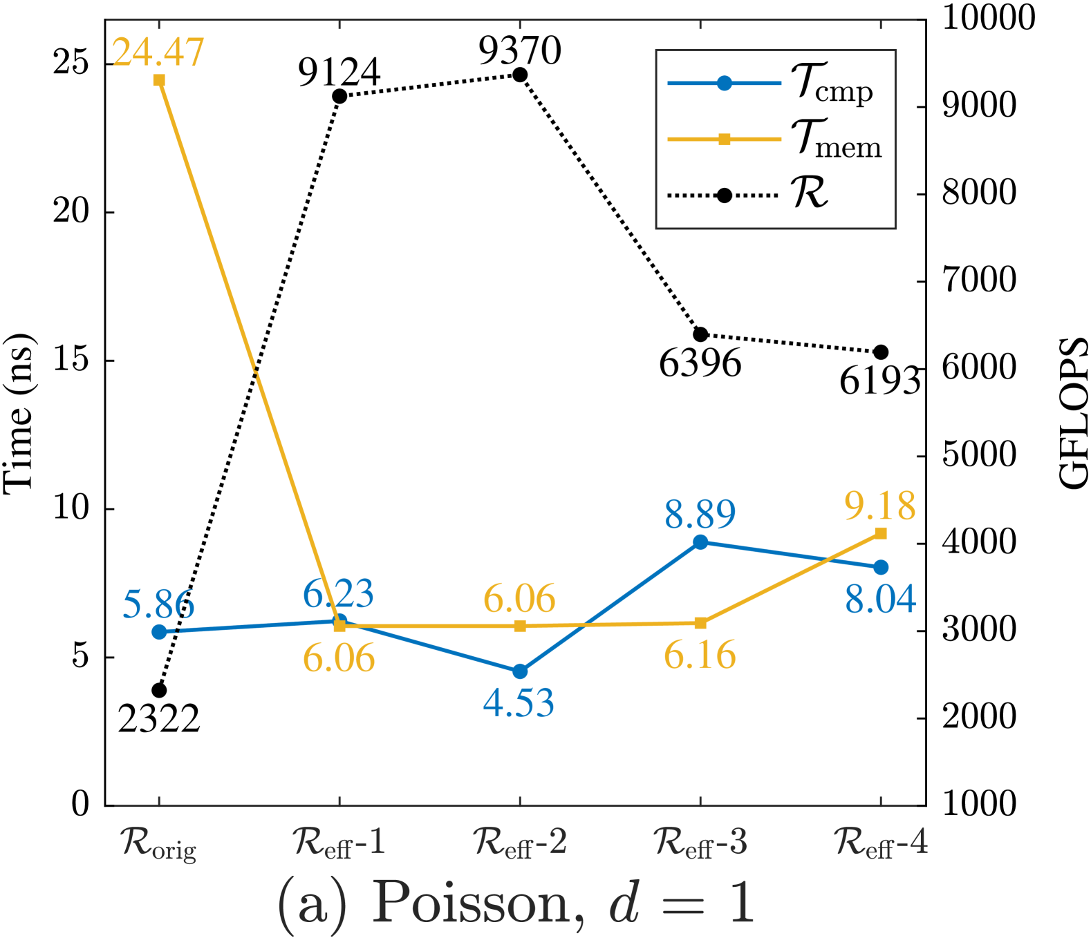
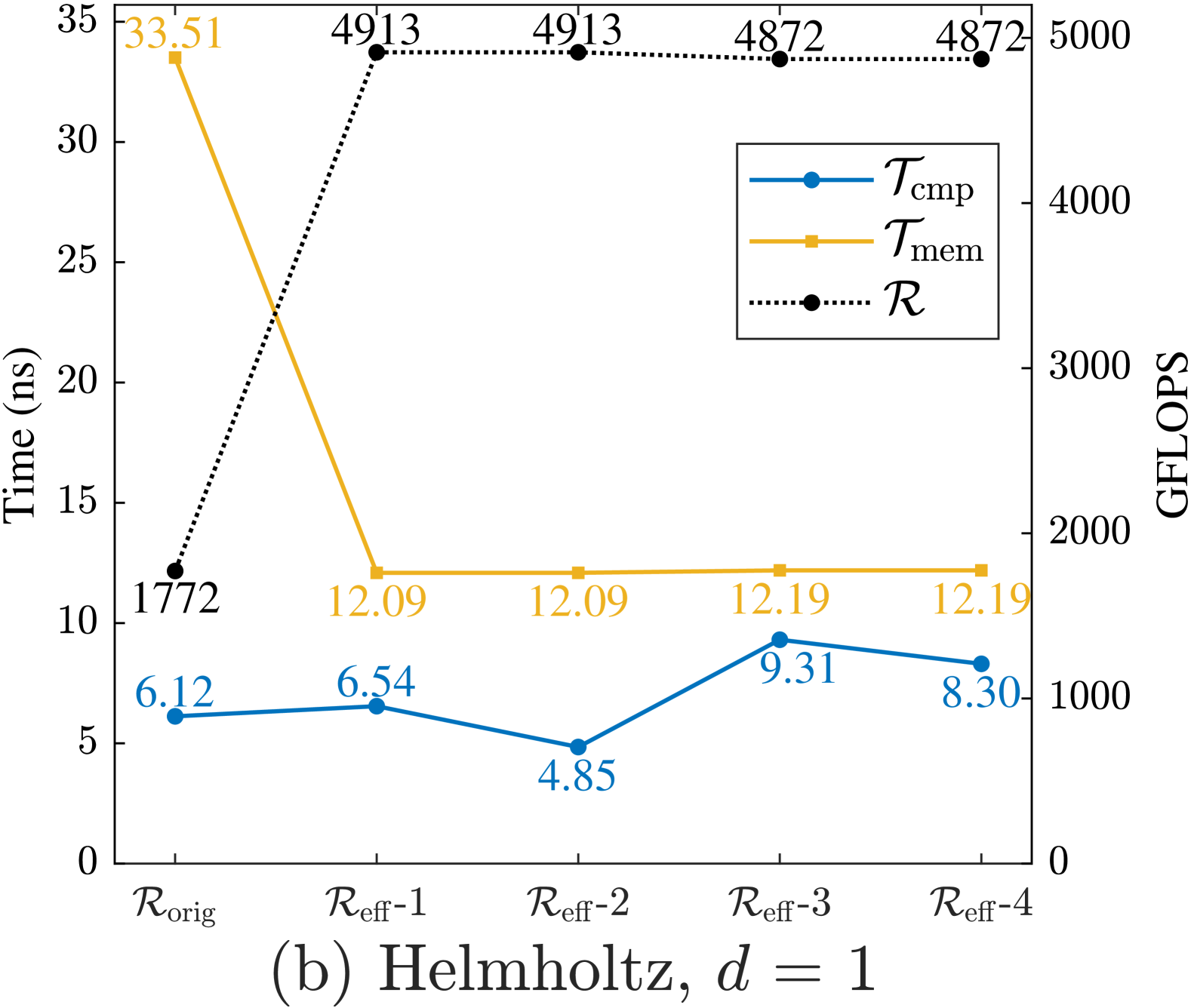
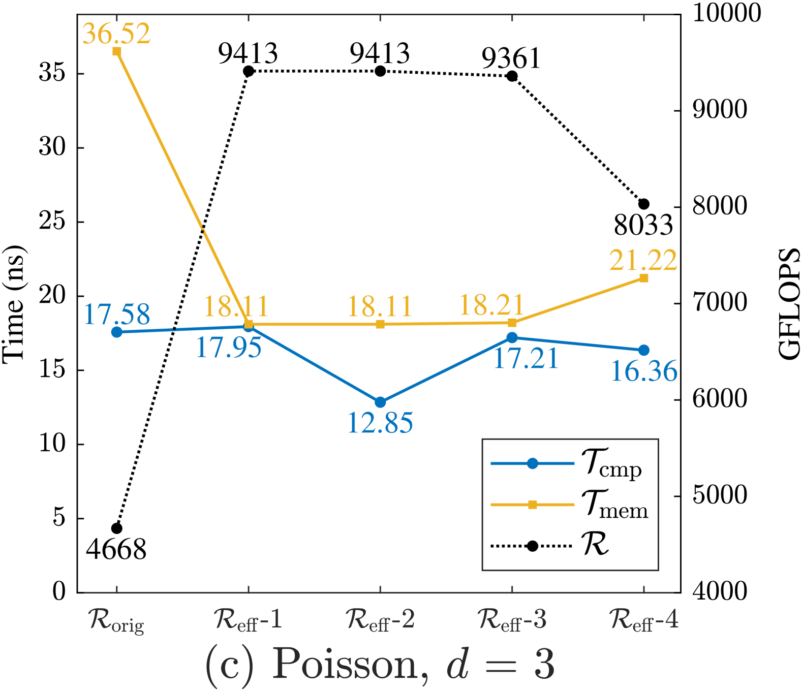
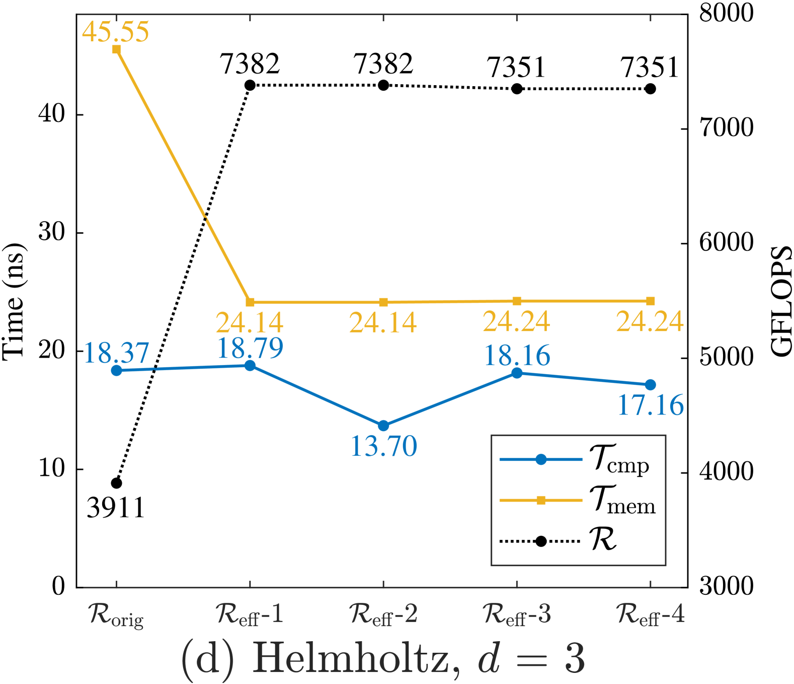
Figure 7. Roofline analysis of axhelm kernels on the NVIDIA A100. $\mathcal{R}_{\mathrm{orig}}$: original kernels, $\mathcal{R}_{\mathrm{eff}}$-1: Algorithm 4, $\mathcal{R}_{\mathrm{eff}}$-2: Algorithm 4 + Tensor Cores, $\mathcal{R}_{\mathrm{eff}}$-3: Algorithm 3 + Tensor Cores, $\mathcal{R}_{\mathrm{eff}}$-4: Algorithm 3 + Tensor Cores + Section 4.1.

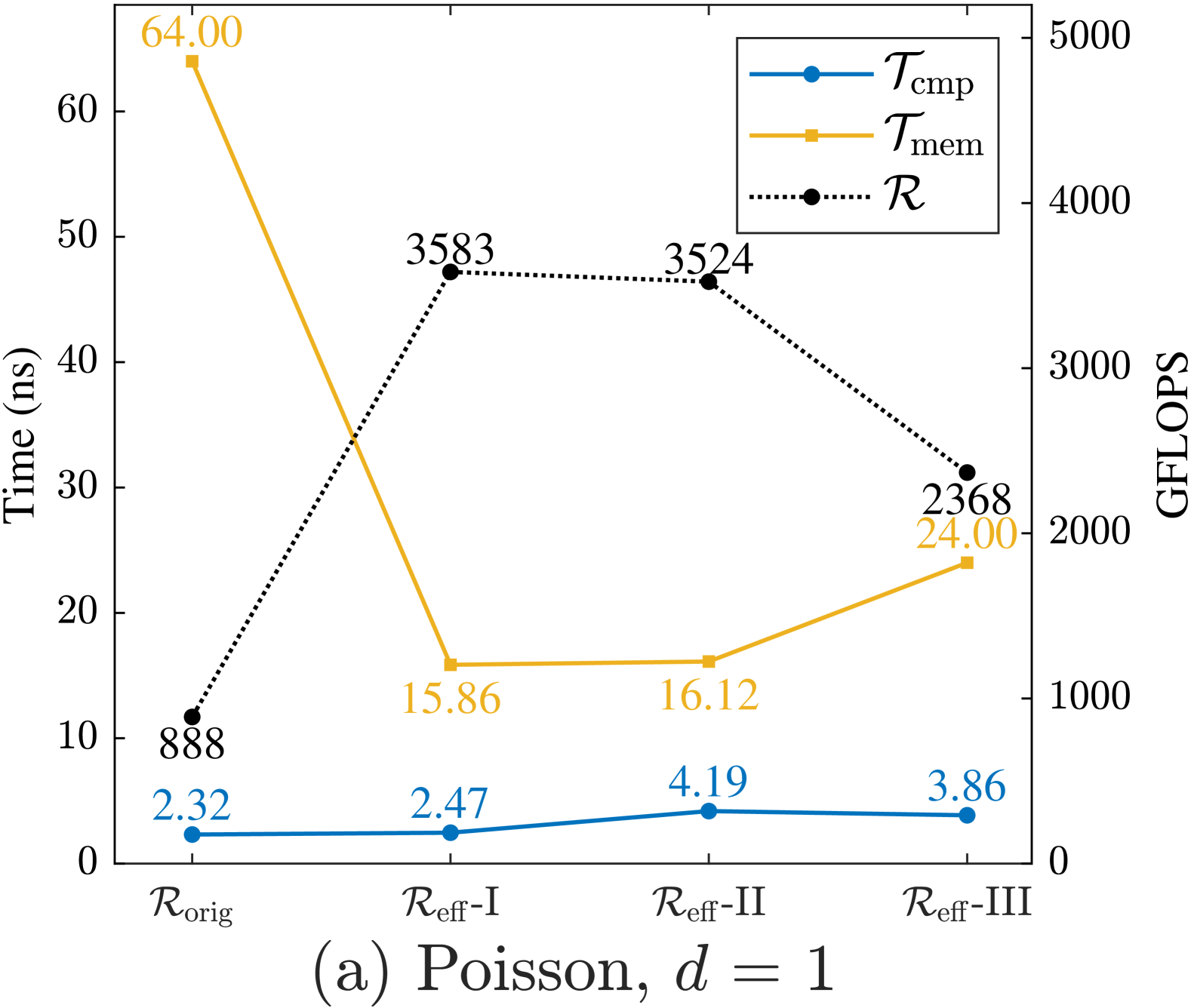
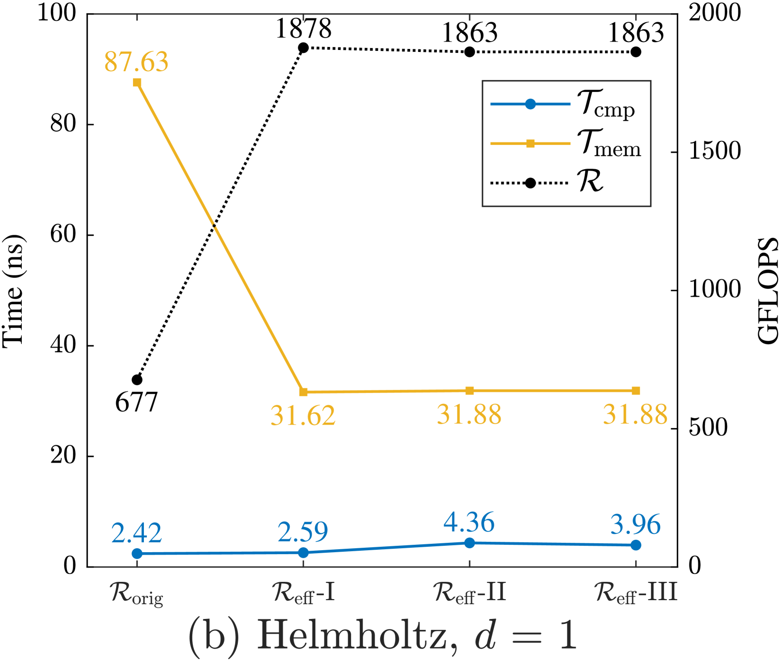
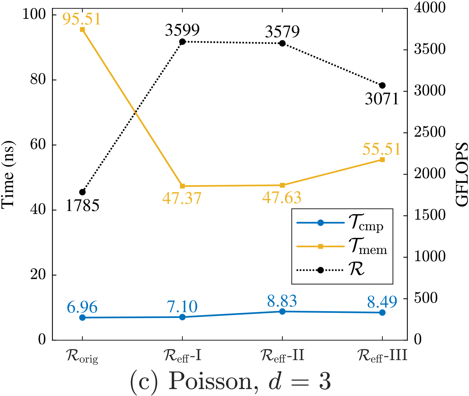
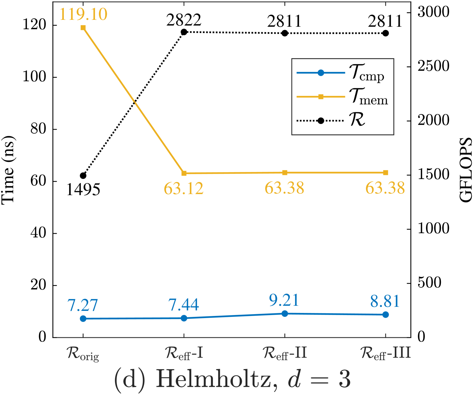
Figure 8. Roofline analysis of axhelm kernels on the DCU K100. $\mathcal{R}_{\mathrm{orig}}$: original kernels, $\mathcal{R}_{\mathrm{eff}}$-$\mathrm{I}$: Algorithm 4, $\mathcal{R}_{\mathrm{eff}}$-$\mathrm{II}$: Algorithm 3, $\mathcal{R}_{\mathrm{eff}}$-$\mathrm{III}$: Algorithm 3 + Section 4.1.

5.3. Performance Evaluation of Tensor Contractions via Parallelepiped

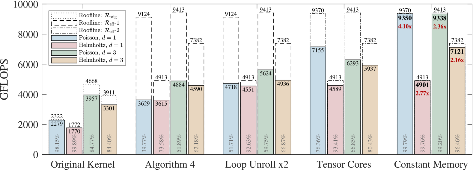
(a) Parallelepiped

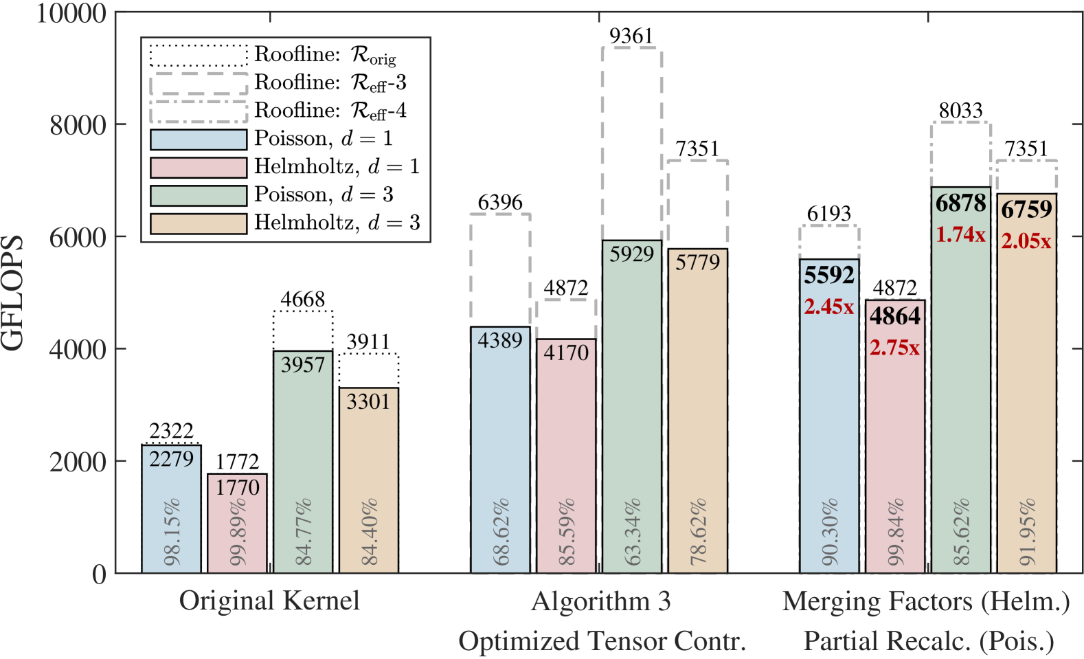
(b) Trilinear

Figure 9. Performance anatomy of axhelm kernels on NVIDIA A100 (best performance in bold).

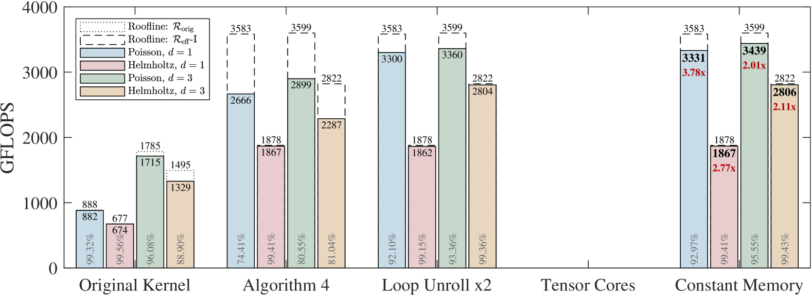
(a) Parallelepiped

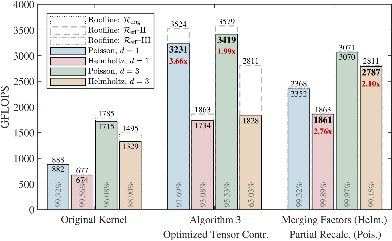
(b) Trilinear

Figure 10. Performance anatomy of axhelm kernels on DCU K100 (best performance in bold).

Despite the limited application of parallelepiped elements in HOSFEM, Algorithm 4 still serves three purposes: 1) It is used for solving problems such as the square cavity flow. 2) It serves to evaluate the performance of tensor contraction. 3) It is used to detect the performance ceiling of HOSFEM on a highly regular mesh.

Figure 9(a) and 10(a) show the performance of the original axhelm kernels and the improvements gained by applying Algorithm 4 and optimizing tensor contraction. The original kernels already exhibit remarkable efficiency, reaching nearly 85% to 100% of $R_{\text{orig}}$. Therefore, even if the computation time for tensor contraction is optimized to zero, overall performance will not see significant improvement without changing the memory access pattern. Despite the improvement in the roofline with Algorithm 4, the actual performance gain does not correspond to the corresponding magnitude. This indicates that, while tensor contraction has undergone a considerable amount of work in optimization, it is still insufficient, with the shortcomings being masked by the original memory accesses.

Optimization strategies for the tensor contraction included loop unrolling, leveraging Tensor Cores (on the A100), and utilizing the constant memory copy of the differentiation matrix were implemented sequentially. These incremental improvements culminated in achieving a roofline efficiency ranging from 92.9% to 99.8%. Compared to the A100, the peak-to-bandwidth ratio of the K100 is significantly higher. Therefore, optimization of computations has a lower necessity for performance improvement. Even without Tensor Cores, performance close to the higher roofline can still be achieved through simple loop unrolling. In a word, the optimization of tensor contraction has reached its limit and can be inherited by axhelm kernels for trilinear elements.

5.4. Performance Evaluation of Axhelm for Trilinear Elements

Figure 9(b) and 10(b) present the performance of the axhelm kernels after incorporating Algorithm 3 and the optimized tensor contraction, followed by an evaluation of the two optimizations outlined in Section 4.1. It is evident that Algorithm 3 and the optimized tensor contraction significantly improve performance. However, for the four cases on the A100 and one case (Helmholtz, $d=3$) on the K100, the performance still leaves some distance to the roofline.

On both platforms, the merging scalar factors optimization elevates the performance of all Helmholtz cases, bringing them close to the roofline. For all Poisson cases, the partial recalculation optimization brings the performance close to a new but lower roofline. On the A100, this optimization yields higher performance, whereas on the K100, the opposite is true. This is because the K100 has a higher peak but lower memory bandwidth, causing the actual performance to be almost entirely limited by memory access.

5.5. Overall Performance Evaluation of Nekbone

Table 6. Nekbone performance evaluation.

Equation Type Axhelm Type GFLOPS GDOFS Accel. Axhelm Error & Iter. Prop. A100-Server, $E$=76$\times$76$\times$76 Poisson, $d=1$ Original 1225 6.51 1x 32% 2.71E-08, 48 Parallelepiped 1594 8.47 1.30x 10% 2.71E-08, 48 Trilinear 1527 8.11 1.25x 16% 2.71E-08, 48 Helmholtz, $d=1$ Original 1208 6.20 1x 35% 2.71E-08, 48 Parallelepiped 1560 7.98 1.29x 16% 2.71E-08, 48 Trilinear 1550 7.93 1.28x 16% 2.71E-08, 48 Poisson, $d=3$ Original 1604 8.53 1x 24% 1.42E-08, 49 Parallelepiped 1857 9.87 1.16x 12% 1.43E-08, 49 Trilinear 1798 9.56 1.12x 16% 1.43E-08, 49 Helmholtz, $d=3$ Original 1616 8.26 1x 25% 1.42E-08, 49 Parallelepiped 1876 9.60 1.16x 13% 1.43E-08, 49 Trilinear 1845 9.44 1.14x 14% 1.43E-08, 49 K100-Server, $E$=112$\times$112$\times$56 Poisson, $d=1$ Original 1019 5.42 1x 35% 4.35E-08, 73 Parallelepiped 1362 7.24 1.33x 12% 4.19E-08, 73 Trilinear 1342 7.14 1.32x 13% 4.19E-08, 73 Helmholtz, $d=1$ Original 978 5.00 1x 45% 4.34E-08, 73 Parallelepiped 1374 7.03 1.40x 22% 4.19E-08, 73 Trilinear 1349 6.90 1.38x 22% 4.19E-08, 73 Poisson, $d=3$ Original 1274 6.78 1x 31% 2.84E-08, 75 Parallelepiped 1518 8.07 1.19x 17% 2.82E-08, 75 Trilinear 1508 8.01 1.18x 18% 2.83E-08, 75 Helmholtz, $d=3$ Original 1271 6.50 1x 33% 2.84E-08, 75 Parallelepiped 1523 7.79 1.20x 18% 2.82E-08, 75 Trilinear 1502 7.68 1.18x 18% 2.86E-08, 75

Table 6 presents the performance results of the Nekbone program, using the optimized axhelm kernels (best-performing version) on both platforms. The axhelm computation time proportion is measured using the hipprof and nsys tools. On the A100 platform, the optimized kernels significantly reduce the time overhead of the axhelm computation and achieve an overall speedup ranging from 1.25x to 1.30x for $d=1$ and from 1.12x to 1.16x for $d=3$. On the K100 platform, the speedup ranges from 1.32x to 1.40x for $d=1$ and from 1.18x to 1.20x for $d=3$. Since the axhelm computation time proportion is higher on the K100 platform and for $d=1$, the overall speedup is also more significant. Additionally, from the perspective of the error term, the optimized axhelm maintains numerical accuracy with no significant deviation from the original implementation. The iteration count (Iter.) remains unchanged, confirming that the optimization strategy does not affect the solver’s convergence.

Although the theoretical FP64 peak of the A100-Server is 39 TFLOPS, which is less than half of the K100-Server’s 98 TFLOPS, the A100-Server achieves higher Nekbone performance and throughput thanks to its higher total bandwidth (1360 GB/s $\times$ 2 ¿ 520 GB/s $\times$ 4). This indicates that the performance of both the axhelm kernel and the Nekbone benchmark is limited by memory access bandwidth.

6. Related Work

The acceleration of finite element solvers on GPGPUs has long been a subject of considerable attention (Göddeke et al., 2007; Cecka et al., 2011; Knepley and Terrel, 2013; Fu et al., 2014). Remacle et al. (Remacle et al., 2016) first proposed a GPU-accelerated algorithm for matrix-free HOSFEM in 2016, using a 3D thread block design, where each thread handles a single node. In 2019, Kasia et al. (Świrydowicz et al., 2019) enhanced the approach by introducing a 2D thread block structure, reducing thread count, supporting larger N values, and optimizing shared memory usage (Karp et al., 2020). LibParanumal, NekRS, and Nekbone have since adopted this approach (Świrydowicz et al., 2019; Karp et al., 2020; Fischer et al., 2022). In 2020, Karp et al. (Karp et al., 2020) integrated the tensor-product optimizations (Świrydowicz et al., 2019) and the hybrid GPU implementation (Gong et al., 2016) into Nekbone. The Nekbone framework’s simplicity has enabled the continuous optimization of the core kernel, axhelm, across various architectures and platforms, achieving near-roofline performance (Brown, 2020; Tsuji et al., 2022; Chalmers et al., 2023; Gong et al., 2016; Markidis et al., 2015).

The concept of recalculating geometric factors on-the-fly was first introduced by Remacle et al. (Remacle et al., 2016) in 2016, followed by several independent implementations (NekRS Team, 2025; Karp et al., 2022b). As shown in Table 4, the high cost of these existing recalculation approaches leads to performance reduction or modest improvements compared to direct access (Remacle et al., 2016; Świrydowicz et al., 2019; Karp et al., 2022a), and effectiveness is limited to low-precision computation on specific platforms where peak performance significantly exceeds bandwidth (Karp et al., 2022b). Consequently, recalculation approaches have been deemed impractical (Świrydowicz et al., 2019) and have received little attention. Most related works focus on optimizing tensor contractions, utilizing direct memory access for geometric factors, while improving their loading efficiency through prefetching/preloading techniques (Karp et al., 2021, 2020; Tsuji et al., 2022) and packed storage formats (Chalmers et al., 2023). Utilizing the 2D thread structure, we extract and decompose the Jacobian matrix’s linear algebraic structure from trilinear elements. We substantially reduce the recalculation cost by extracting invariant and common terms, thereby achieving a notable improvement in roofline performance. The higher roofline demonstrates that, despite long-standing optimizations of tensor contractions, their potential has not been fully realized. Through careful optimizations, including merging scalar factors, partial recalculation, Tensor Core acceleration, and constant memory utilization, performance approaches the new roofline.

7. Conclusion

Previous optimizations of the axhelm kernel have pushed its performance close to the roofline limit. Further improvements hinge on obtaining geometric factors at a truly low cost. As an extension of matrix-free methods, the efficient on-the-fly recalculation of geometric factors can significantly unlock the performance potential. Equally important, a series of optimizations targeting tensor contractions, including Tensor Core acceleration, constant memory storage for HOSFEM constants, and other techniques, can push the performance closer to the higher roofline. These improvements highlight HOSFEM’s strong compatibility with modern accelerator architectures, as well as its untapped and underestimated performance potential. Future research will focus on: 1) Element-type-adaptive kernels. 2) Other kernels that require access to geometric factors. 3) Integration of the proposed optimizations into practical applications, such as NekRS. Meanwhile, we will also explore different polynomial orders and low/mixed-precision implementations.

References

- (1)
- Anderson et al. (2021) Robert Anderson, Julian Andrej, Andrew Barker, Jamie Bramwell, Jean-Sylvain Camier, Jakub Cerveny, Veselin Dobrev, Yohann Dudouit, Aaron Fisher, Tzanio Kolev, Will Pazner, Mark Stowell, Vladimir Tomov, Ido Akkerman, Johann Dahm, David Medina, and Stefano Zampini. 2021. MFEM: A modular finite element methods library. Computers & Mathematics with Applications 81 (2021), 42–74. https://doi.org/10.1016/j.camwa.2020.06.009.
- Brown (2020) Nick Brown. 2020. Exploring the acceleration of Nekbone on reconfigurable architectures. In 2020 IEEE/ACM International Workshop on Heterogeneous High-performance Reconfigurable Computing (H2RC). IEEE, GA, USA, 19–28. https://doi.org/10.1109/H2RC51942.2020.00008.
- Cecka et al. (2011) Cris Cecka, Adrian J. Lew, and E. Darve. 2011. Assembly of finite element methods on graphics processors. Internat. J. Numer. Methods Engrg. 85, 5 (2011), 640–669. https://doi.org/10.1002/nme.2989.
- CEED Team (2025a) CEED Team. 2025a. CEED Bake-off Problems (Benchmarks). https://ceed.exascaleproject.org/bps/. (Accessed 2 April 2025).
- CEED Team (2025b) CEED Team. 2025b. Center for Efficient Exascale Discretizations (CEED). https://ceed.exascaleproject.org/. (Accessed 13 January 2025).
- Chalmers et al. (2023) Noel Chalmers, Abhishek Mishra, Damon McDougall, and Tim Warburton. 2023. HipBone: A performance-portable graphics processing unit-accelerated C++ version of the NekBone benchmark. The International Journal of High Performance Computing Applications 37, 5 (2023), 560–577. https://doi.org/10.1177/10943420231178552.
- Chen et al. (2025) Yanxiang Chen, Pablo de Oliveira Castro, Paolo Bientinesi, and Roman Iakymchuk. 2025. Enabling mixed-precision with the help of tools: A Nekbone case study. In Parallel Processing and Applied Mathematics. Springer Nature Switzerland, Cham, 34–50. https://doi.org/10.1007/978-3-031-85697-6_3.
- Cifuentes and Kalbag (1992) A.O. Cifuentes and A. Kalbag. 1992. A performance study of tetrahedral and hexahedral elements in 3-D finite element structural analysis. Finite Elements in Analysis and Design 12, 3 (1992), 313–318. https://doi.org/10.1016/0168-874X(92)90040-J.
- CORAL Team (2025) CORAL Team. 2025. CORAL-2 Benchmarks. https://asc.llnl.gov/coral-2-benchmarks. (Accessed 2 April 2025).
- Fischer et al. (2022) Paul Fischer, Stefan Kerkemeier, Misun Min, Yu-Hsiang Lan, Malachi Phillips, Thilina Rathnayake, Elia Merzari, Ananias Tomboulides, Ali Karakus, Noel Chalmers, and Tim Warburton. 2022. NekRS, a GPU-accelerated spectral element Navier-Stokes solver. Parallel Comput. 114 (2022), 102982. https://doi.org/10.1016/j.parco.2022.102982.
- Fischer et al. (2025) Paul Fischer, Stefan Kerkemeier, Ananias Tomboulides, Misun Min, Elia Merzari, Aleksandr Obabko, Dillon Shaver, Thilina Ratnayaka, and YuHsiang Lan. 2025. NEK, fast high-order scalable CFD. https://nek5000.mcs.anl.gov/. (Accessed 13 January 2025).
- Fischer et al. (2020) Paul Fischer, Misun Min, Thilina Rathnayake, Som Dutta, Tzanio Kolev, Veselin Dobrev, Jean-Sylvain Camier, Martin Kronbichler, Tim Warburton, Kasia Świrydowicz, and Jed Brown. 2020. Scalability of high-performance PDE solvers. The International Journal of High Performance Computing Applications 34, 5 (2020), 562–586. https://doi.org/10.1177/1094342020915762.
- Fu et al. (2014) Zhisong Fu, T. James Lewis, Robert M. Kirby, and Ross T. Whitaker. 2014. Architecting the finite element method pipeline for the GPU. J. Comput. Appl. Math. 257 (2014), 195–211. https://doi.org/10.1016/j.cam.2013.09.001.
- Gong et al. (2016) Jing Gong, Stefano Markidis, Erwin Laure, Matthew Otten, Paul Fischer, and Misun Min. 2016. Nekbone performance on GPUs with OpenACC and CUDA Fortran implementations. The Journal of Supercomputing 72, 11 (2016), 4160–4180. https://doi.org/10.1007/s11227-016-1744-5.
- Göddeke et al. (2007) Dominik Göddeke, Robert Strzodka, Jamaludin Mohd-Yusof, Patrick McCormick, Sven H.M. Buijssen, Matthias Grajewski, and Stefan Turek. 2007. Exploring weak scalability for FEM calculations on a GPU-enhanced cluster. Parallel Comput. 33, 10 (2007), 685–699. https://doi.org/10.1016/j.parco.2007.09.002.
- Huang and Chen (2015) Kun Huang and Yifeng Chen. 2015. Improving performance of floating point division on GPU and MIC. In Algorithms and Architectures for Parallel Processing, Guojun Wang, Albert Zomaya, Gregorio Martinez, and Kenli Li (Eds.). Springer International Publishing, Cham, 691–703. https://doi.org/10.1007/978-3-319-27122-4_48.
- Ilic and Notaros (2001) M.M. Ilic and B.M. Notaros. 2001. Trilinear hexahedral finite elements with higher-order polynomial field expansions for hybrid SIE/FE large-domain electromagnetic modeling. In IEEE Antennas and Propagation Society International Symposium. 2001 Digest. Held in conjunction with: USNC/URSI National Radio Science Meeting (Cat. No.01CH37229), Vol. 3. IEEE, Boston, MA, USA, 192–195. https://doi.org/10.1109/APS.2001.960065.
- Ilic and Notaros (2003) M.M. Ilic and B.M. Notaros. 2003. Higher order hierarchical curved hexahedral vector finite elements for electromagnetic modeling. IEEE Transactions on Microwave Theory and Techniques 51, 3 (2003), 1026–1033. https://doi.org/10.1109/TMTT.2003.808680.
- Ivanov et al. (2015) Ilya Ivanov, Jing Gong, Dana Akhmetova, Ivy Bo Peng, Stefano Markidis, Erwin Laure, Rui Machado, Mirko Rahn, Valeria Bartsch, Alistair Hart, and Paul Fischer. 2015. Evaluation of parallel communication models in Nekbone, a Nek5000 mini-application. In 2015 IEEE International Conference on Cluster Computing (CLUSTER). IEEE, Chicago, IL, USA, 760–767. https://doi.org/10.1109/CLUSTER.2015.131.
- Jackson et al. (2020) Adrian Jackson, Michèle Weiland, Nick Brown, Andrew Turner, and Mark Parsons. 2020. Investigating applications on the A64FX. In 2020 IEEE International Conference on Cluster Computing (CLUSTER). IEEE, Kobe, Japan, 549–558. https://doi.org/10.1109/CLUSTER49012.2020.00078.
- Jansson et al. (2023) Niclas Jansson, Martin Karp, Adalberto Perez, Timofey Mukha, Yi Ju, Jiahui Liu, Szilárd Páll, Erwin Laure, Tino Weinkauf, Jörg Schumacher, Philipp Schlatter, and Stefano Markidis. 2023. Exploring the ultimate regime of turbulent Rayleigh-Bénard convection through unprecedented spectral-element simulations. In Proceedings of the International Conference for High Performance Computing, Networking, Storage and Analysis (Denver, CO, USA) (SC’23). Association for Computing Machinery, New York, NY, USA, Article 5, 9 pages. https://doi.org/10.1145/3581784.3627039.
- Jansson et al. (2024) Niclas Jansson, Martin Karp, Artur Podobas, Stefano Markidis, and Philipp Schlatter. 2024. Neko: A modern, portable, and scalable framework for high-fidelity computational fluid dynamics. Computers & Fluids 275 (2024), 106243. https://doi.org/10.1016/j.compfluid.2024.106243.
- Karp et al. (2020) Martin Karp, Niclas Jansson, Artur Podobas, Philipp Schlatter, and Stefano Markidis. 2020. Optimization of tensor-product operations in Nekbone on GPUs. (2020). Poster presented at the International Conference for High Performance Computing, Networking, Storage and Analysis (SC’20 Poster) https://sc20.supercomputing.org/proceedings/tech_poster/tech_poster_pages/rpost115.html.
- Karp et al. (2022a) Martin Karp, Niclas Jansson, Artur Podobas, Philipp Schlatter, and Stefano Markidis. 2022a. Reducing communication in the conjugate gradient method: a case study on high-order finite elements. In Proceedings of the Platform for Advanced Scientific Computing Conference (Basel, Switzerland) (PASC’22). Association for Computing Machinery, New York, NY, USA, Article 2, 11 pages. https://doi.org/10.1145/3539781.3539785.
- Karp et al. (2023) Martin Karp, Daniele Massaro, Niclas Jansson, Alistair Hart, Jacob Wahlgren, Philipp Schlatter, and Stefano Markidis. 2023. Large-scale direct numerical simulations of turbulence using GPUs and modern Fortran. The International Journal of High Performance Computing Applications 37, 5 (2023), 487–502. https://doi.org/10.1177/10943420231158616.
- Karp et al. (2021) Martin Karp, Artur Podobas, Niclas Jansson, Tobias Kenter, Christian Plessl, Philipp Schlatter, and Stefano Markidis. 2021. High-performance spectral element methods on Field-Programmable Gate Arrays : implementation, evaluation, and future projection. In 2021 IEEE International Parallel and Distributed Processing Symposium (IPDPS). IEEE, Portland, OR, USA, 1077–1086. https://doi.org/10.1109/IPDPS49936.2021.00116.
- Karp et al. (2022b) Martin Karp, Artur Podobas, Tobias Kenter, Niclas Jansson, Christian Plessl, Philipp Schlatter, and Stefano Markidis. 2022b. A high-fidelity flow solver for unstructured meshes on Field-Programmable Gate Arrays: design, evaluation, and future challenges. In International Conference on High Performance Computing in Asia-Pacific Region (Virtual Event, Japan) (HPCAsia’22). Association for Computing Machinery, New York, NY, USA, 125–136. https://doi.org/10.1145/3492805.3492808.
- Knepley and Terrel (2013) Matthew G. Knepley and Andy R. Terrel. 2013. Finite element integration on GPUs. ACM Trans. Math. Softw. 39, 2, Article 10 (2013), 13 pages. https://doi.org/10.1145/2427023.2427027.
- Kolda and Bader (2009) Tamara G. Kolda and Brett W. Bader. 2009. Tensor decompositions and applications. SIAM Rev. 51, 3 (2009), 455–500. https://doi.org/10.1137/07070111X.
- Korelc and Wriggers (1996) J. Korelc and P. Wriggers. 1996. An efficient 3D enhanced strain element with Taylor expansion of the shape functions. Computational Mechanics 19 (1996), 30–40. https://doi.org/10.1007/BF02757781.
- Liao et al. (2021) Heng Liao, Jiajin Tu, Jing Xia, Hu Liu, Xiping Zhou, Honghui Yuan, and Yuxing Hu. 2021. Ascend: a scalable and unified architecture for ubiquitous deep neural network computing : industry track paper. In 2021 IEEE International Symposium on High-Performance Computer Architecture (HPCA). IEEE, Seoul, Korea (South), 789–801. {https://doi.org/10.1109/HPCA51647.2021.00071}.
- M. O. Deville et al. (2003) M. O. Deville, P. F. Fischer, and E. H. Mund. 2003. High-Order methods for incompressible fluid flow. Applied Mechanics Reviews 56, 3 (2003), B43–B43. https://doi.org/10.1115/1.1566402.
- Markidis et al. (2018) Stefano Markidis, Steven Wei Der Chien, Erwin Laure, Ivy Bo Peng, and Jeffrey S. Vetter. 2018. NVIDIA Tensor Core programmability, performance & precision. In 2018 IEEE International Parallel and Distributed Processing Symposium Workshops (IPDPSW). IEEE, Vancouver, BC, Canada, 522–531. https://doi.org/10.1109/IPDPSW.2018.00091.
- Markidis et al. (2015) Stefano Markidis, Jing Gong, Michael Schliephake, Erwin Laure, Alistair Hart, David Henty, Katherine Heisey, and Paul Fischer. 2015. OpenACC acceleration of the Nek5000 spectral element code. The International Journal of High Performance Computing Applications 29, 3 (2015), 311–319. https://doi.org/10.1177/1094342015576846.
- Merzari et al. (2023) Elia Merzari, Steven Hamilton, Thomas Evans, Misun Min, Paul Fischer, Stefan Kerkemeier, Jun Fang, Paul Romano, Yu-Hsiang Lan, Malachi Phillips, Elliott Biondo, Katherine Royston, Tim Warburton, Noel Chalmers, and Thilina Rathnayake. 2023. Exascale multiphysics nuclear reactor simulations for advanced designs. In SC23: International Conference for High Performance Computing, Networking, Storage and Analysis. Association for Computing Machinery, DENVER, CO, USA, 1–11. https://doi.org/10.1145/3581784.3627038.
- Min et al. (2024) Misun Min, Michael Brazell, Ananias Tomboulides, Matthew Churchfield, Paul Fischer, and Michael Sprague. 2024. Towards exascale for wind energy simulations. The International Journal of High Performance Computing Applications 38, 4 (2024), 337–355. https://doi.org/10.1177/10943420241252511.
- Min et al. (2022) Misun Min, Yu-Hsiang Lan, Paul Fischer, Elia Merzari, Stefan Kerkemeier, Malachi Phillips, Thilina Rathnayake, April Novak, Derek Gaston, Noel Chalmers, and Tim Warburton. 2022. Optimization of full-core reactor simulations on Summit. In SC22: International Conference for High Performance Computing, Networking, Storage and Analysis. IEEE, Dallas, TX, USA, 1–11. https://doi.org/10.1109/SC41404.2022.00079.
- Min et al. (2025) Misun Min, Yu-Hsiang Lan, Paul Fischer, Thilina Rathnayake, and John Holmen. 2025. Nek5000/RS performance on advanced GPU architectures. Frontiers in High Performance Computing 2 (2025), 1–15. https://doi.org/10.3389/fhpcp.2024.1303358.
- Nek5000 Team (2025) Nek5000 Team. 2025. nekBench. https://github.com/Nek5000/nekBench. (Accessed 9 April 2025).
- NekRS Team (2025) NekRS Team. 2025. NekRS. https://github.com/Nek5000/nekRS. (Accessed 13 January 2025).
- Project (2025) Exascale Computing Project. 2025. Exascale Computing Project. https://www.exascaleproject.org/. (Accessed 2 April 2025).
- Remacle et al. (2016) J.-F. Remacle, R. Gandham, and T. Warburton. 2016. GPU accelerated spectral finite elements on all-hex meshes. J. Comput. Phys. 324 (2016), 246–257. https://doi.org/10.1016/j.jcp.2016.08.005.
- Schieffer et al. (2024) Gabin Schieffer, Daniel Araújo De Medeiros, Jennifer Faj, Aniruddha Marathe, and Ivy Peng. 2024. On the rise of AMD Matrix Cores: performance, power efficiency, and programmability. In 2024 IEEE International Symposium on Performance Analysis of Systems and Software (ISPASS). IEEE, Indianapolis, IN, USA, 132–143. https://doi.org/10.1109/ISPASS61541.2024.00022.
- Schneider et al. (2019) Teseo Schneider, Jérémie Dumas, Xifeng Gao, Mario Botsch, Daniele Panozzo, and Denis Zorin. 2019. Poly-Spline Finite-Element Method. ACM Trans. Graph. 38, 3, Article 19 (2019), 16 pages. https://doi.org/10.1145/3313797.
- Simo et al. (1993) J.C Simo, F Armero, and R.L Taylor. 1993. Improved versions of assumed enhanced strain tri-linear elements for 3D finite deformation problems. Computer Methods in Applied Mechanics and Engineering 110, 3 (1993), 359–386. https://doi.org/10.1016/0045-7825(93)90215-J.
- Team (2025a) MFEM Team. 2025a. MFEM: modular finite element methods library. https://mfem.org/. (Accessed 13 January 2025).
- Team (2025b) Parallel Numerical Algorithms Research Team. 2025b. libParanumal: library of parallel numerical algorithms for high-Order finite element methods. https://www.paranumal.com/software. (Accessed 2 April 2025).
- Team (2025c) VisIt Development Team. 2025c. VisIt: An Open-Source Visualization Tool. https://visit-dav.github.io/visit-website/index.html. (Accessed 19 March 2025).
- Tsuji et al. (2022) Miwako Tsuji, Misun Min, Stefan Kerkemeier, Paul Fischer, Elia Merzari, and Mitsuhisa Sato. 2022. Performance tuning of the Helmholtz matrix-vector product kernel in the computational fluid dynamics solver Nek5000/RS for the A64FX processor. In International Conference on High Performance Computing in Asia-Pacific Region Workshops (Virtual Event, Japan) (HPCAsia ’22 Workshops). Association for Computing Machinery, New York, NY, USA, 49–59. https://doi.org/10.1145/3503470.3503476.
- Williams et al. (2009) Samuel Williams, Andrew Waterman, and David Patterson. 2009. Roofline: an insightful visual performance model for multicore architectures. Commun. ACM 52, 4 (2009), 65–76. https://doi.org/10.1145/1498765.1498785.
- Świrydowicz et al. (2019) Kasia Świrydowicz, Noel Chalmers, Ali Karakus, and Tim Warburton. 2019. Acceleration of tensor-product operations for high-order finite element methods. The International Journal of High Performance Computing Applications 33, 4 (2019), 735–757. https://doi.org/10.1177/1094342018816368.