Restoring the Forecasting Power of Google Trends
with Statistical Preprocessing

Abstract

Google Trends reports how frequently specific queries are searched on Google over time. It is widely used in research and industry to gain early insights into public interest. However, its data generation mechanism introduces missing values, sampling variability, noise, and trends. These issues arise from privacy thresholds mapping low search volumes to zeros, daily sampling variations causing discrepancies across historical downloads, and algorithm updates altering volume magnitudes over time. Data quality has recently deteriorated, with more zeros and noise, even for previously stable queries. We propose a comprehensive statistical methodology to preprocess Google Trends search information using hierarchical clustering, smoothing splines, and detrending. We validate our approach by forecasting U.S. influenza hospitalizations with a univariate ARIMAX model. Compared to omitting exogenous variables, our results show that raw Google Trends data degrades modeling performance, while preprocessed signals enhance forecast accuracy by 58% nationally and 24% at the state level.

Keywords: Google Trends, Preprocessing, Clustering, Denoising, Detrending, ARIMAX

1 Introduction

The digital footprint generated by billions of daily online searches offers a wealth of data, capturing public interests and behaviors across a broad range of topics. As the world’s leading search engine, Google plays a central role in this ecosystem, with Google Trends emerging as a powerful, public-facing tool for gaining early insights into evolving patterns. Over the past two decades, Google Trends has been successfully applied in various fields, including epidemiology to predict infectious diseases and outbreaks (Yang et al. 2015), macroeconomics to forecast unemployment rates (D’Amuri & Marcucci 2017), finance to analyze stock market trends (Preis et al. 2013), and marketing to study consumer behavior in fashion (Silva et al. 2019). Compared to traditional data sources such as surveys, these aggregated search volumes are low-cost, continuously updated, and can provide a more dynamic and accurate representation of how behaviors, opinions, and sentiments evolve over time (Stephens-Davidowitz 2017).

Google Trends provides aggregated search volumes for specific keywords across various geographic scales and time periods. Despite its extensive adoption, the quality of the data presents significant challenges that can affect the reliability of models built on it. Missing values, sampling variability, noise, and unexpected long-term trends arise from the data generation process. For example, privacy-preserving thresholds enforce zero values when searches are too sparse in a region to maintain user anonymity. Daily variations due to Google Trends’ sampling methods introduce noticeable discrepancies across data downloads, which may appear as noise in the reported search volumes. Algorithm updates can affect data consistency over time, resulting in search volumes with different prevalence of zeros, noise levels, and magnitudes that may not reflect meaningful shifts in search patterns. For current and future users of Google trends data, understanding and addressing these issues is critical for unlocking its full potential and enhancing the reliability of models leveraging search data.

1.1 Related Work

Although there is extensive research on the use of Google Trends data for multiple applications, only a few recent analyses have focused on quantifying and addressing data quality issues. Some studies suggest removing all queries whose time series have missing values from the analysis (Cebrián & Domenech 2023, Liu et al. 2015), resulting in a potential loss of valuable information. To mitigate this, Neumann et al. (2023) recommend combining search phrases in the Google Trends tool using the Boolean operator OR (“+”), which allows the retrieval of aggregated search volumes. However, their approach does not describe how to effectively construct these combinations, leaving a gap in practical implementation.

Sampling variability is another area of concern in Google Trends data. In Cebrián & Domenech (2023), the authors highlight that the lack of accuracy in Google Trends data originates from the sampling process, but do not propose specific methods to improve data quality. In contrast, Eichenauer et al. (2022) and Neumann et al. (2023) explain the Google Trends sampling mechanism, which introduces noise and fluctuations in the returned search volumes, and suggest averaging results from multiple downloads to reduce these variations. Expanding on this, Cebrián & Domenech (2024) model and simulate the data generation process to better understand sampling error, proposing a measure to determine the number of samples required for consistent search volumes. However, since Google servers cache query results and return identical values for repeated requests within a 24-hour period, averaging multiple samples may not be practical for real-time analysis.

Several studies have applied temporal smoothing techniques to preprocess Google Trends data before integrating it into forecasting models. For instance, moving averages are employed to smooth time series of search volumes (Liu et al. 2015, Rabiolo et al. 2021, Wang et al. 2022, Lampos et al. 2021). However, this method can introduce phase shifts, particularly for weekly or monthly data where the peak is delayed after smoothing. Alternatively, Silva et al. (2019) utilize singular spectrum analysis to denoise search data, demonstrating its effectiveness in enhancing the performance of a neural network autoregression forecasting model. Similarly, Fenga (2020) combines a Seasonal AutoRegressive Integrated Moving Average (SARIMA) model with a wavelet denoising filter, showing that the addition of the filter improves forecasting accuracy compared to using SARIMA alone. While these studies effectively address noisy signals and underscore the benefits of denoising Google Trends data to enhance forecasts, their methodologies rely on the entire time series for smoothing, including future time periods. This makes them unsuitable for real-time forecasting, as future data is not available at the time of prediction. Retrospective application of these techniques could introduce future-looking information, potentially leading to unrealistic accuracy improvements not achievable in real-time settings.

Various online blog case studies also explore methods for analyzing and potentially enhancing Google Trends data. For instance, Matsa et al. (2017) suggest retrieving search volumes of terms grouped into broad categories using domain knowledge, imputing the remaining zeros with regression, and smoothing fluctuations with a generalized additive model. Their methodology, while comprehensive, lacks reproducibility due to the manual selection and combination of keywords and the need for multiple Google accounts to circumvent data download limits.

Clustering semantically related terms as a preprocessing step has also been explored. Ning et al. (2024) group semantically related search queries using hierarchical clustering based on correlation distance. A group-wise L2 penalty is applied to these clusters, allowing the model to retain or eliminate entire sets of terms. However, while clustering queries that share meaning is beneficial, the group-wise penalty may inadvertently discard individual terms within clusters that have strong predictive power, potentially overlooking valuable information. Similarly, Lampos et al. (2015) use k-means clustering with cosine similarity to group queries that share semantic and temporal patterns. However, the number of clusters for k-means needs to be specified in advance, which can be challenging without first analyzing the cluster structure.

One of the earliest and most significant applications of Google Trends has been infectious disease forecasting in the United States (US). Inspired by its prior successes, influenza activity prediction at the national and state levels in the US serves as a case study to demonstrate the effectiveness of our Google Trends data preprocessing methodology. The first documented use of Google search data was presented by Ginsberg et al. (2009), who leveraged search volumes to forecast influenza outbreaks, leading to the development of Google Flu Trends (GFT) tool. Following the failure of GFT to provide reliable forecasts (Santillana et al. 2014), substantial research has been conducted on refining Google Trends-based predictions by integrating data from multiple sources and calibrating machine learning models (Yang et al. 2017, Kandula et al. 2019, Ning et al. 2019, Yang et al. 2021). In particular, Yang et al. (2015) improved the GFT framework with ARGO (AutoRegression with GOogle search data), an autoregressive model with LASSO regularization that accurately estimates influenza-like illness (ILI) rates based on historical flu activity and Google search data. Building on this, Ning et al. (2019) developed ARGO2 (2-step Augmented Regression with GOogle data), which refines ARGO by combining national and regional predictions, incorporating cross-regional correlations, and computing the final ILI estimates using the best linear predictor. The performance of these models shows the benefits of integrating Google Trends data in predictive models applied to influenza forecasting.

1.2 Our contributions

In this paper, we present a preprocessing methodology designed to enhance the quality of Google Trends data for real-time forecasting applications. Our approach addresses key challenges inherent in search data, such as missing values, sampling variability, noise, and trends, thereby improving its consistency, stability, and predictive utility. This reproducible framework refines Google Trends data into more reliable and informative features for prediction tasks.

We begin with a practical overview of Google Trends, highlighting its functionalities, challenges, and strategies for selecting relevant search queries. Our statistical methodology is then presented in three stages. (1) First, we employ hierarchical clustering to group similar keywords based on correlations between their time series. Combined search volumes of related terms overcome Google’s privacy thresholds, yielding non-zero values for initially sparse data, thus reducing missing values and stabilizing sampling variability. (2) Next, we apply smoothing splines iteratively to denoise the time series without introducing look-ahead bias, preserving the integrity necessary for real-time forecasting models. This step effectively reduces noise caused by daily sampling variations and short-term fluctuations in searches. (3) To further improve data quality, we use linear detrending, quadratic detrending, and differencing to eliminate long-term deterministic and stochastic trends, ensuring stationarity in the time series while preserving short-term dynamics. We then use correlations between the resulting predictors and the target variables to filter and retain only the most relevant search queries.

We validate our preprocessing framework through its application to predicting influenza hospitalizations in the United States using an AutoRegressive Integrated Moving Average with eXogenous variables (ARIMAX) model, incorporating Google Trends data as external predictors. Our results show that using preprocessed search data significantly enhances prediction accuracy compared to omitting external variables entirely, while using raw data degrades performance. Although our case study focuses on infectious disease forecasting, the proposed approach is designed as a general-purpose framework for preprocessing Google Trends data, making it suitable for a wide range of domains.

2 Data

Google Trends is the primary data source for this study, providing search volumes for flu-related terms. Available publicly at https://trends.google.com/trends/, it offers valuable insights into search behaviors but presents challenges due to its data generation mechanism. For an end-to-end application of our preprocessing methodology, we supplement this data with influenza hospital admission counts from the U.S. Centers for Disease Control and Prevention (CDC).

2.1 Description of Google Trends

Google Trends allows users to analyze search behavior for inputted keywords by location, time range, category and search type. The search volume is available for two types of keywords: “search terms” and “topics”. A search term can be a single word or a phrase, with returned volumes encompassing searches that include the words in any order, as well as with additional words before or after. Boolean logic can be used to retrieve specific phrases or exclude some terms (Trends Help 2025d). Topics are broader than search terms and typically yield higher search volumes. They are “generally considered to be more reliable for Google Trends data” (Google News Initiative 2025), as they account for all languages and spellings of a word. Moreover, results for topics are more refined and less noisy, as these are associated with a category (such as “Health” or “Finance”), which returns results in the desired field when a term has multiple meanings (Trends Help 2025c).

In fact, the tool allows to refine the search to only include results for a particular area of interest or “category”, rather than including all searches. The category then works as a filter for the data, to exclude irrelevant searches. As another filter, there are different “search types”, e.g., web search or Youtube search. In this paper, we analyze web searches, which is the case of most studies. Results can be obtained for any location, ranging from worldwide to a particular country, state, metro, or city. Data is available for any time range from 2004 to the present.

For a specific search, there are four types of data representations: “interest over time”, “interest by subregion”,“related queries” and “related topics”. The “interest over time” feature returns a time series of search volumes that reflects the relative popularity of a keyword over time, scaled from 0 to 100, where 100 corresponds to the peak volume (Trends Help 2025a). This time series reveals trends, seasonal patterns, or spikes in interest, and can be obtained at various temporal resolutions, e.g., hourly, daily, weekly or monthly. Figure 1 displays a representative example of search volumes for the keyword “Cough”. “Interest by subregion” provides a geographical breakdown of search data, highlighting the areas where a subject is most popular. By explicitly selecting a location in the input box, the interest over time also provides the interest in that particular region.

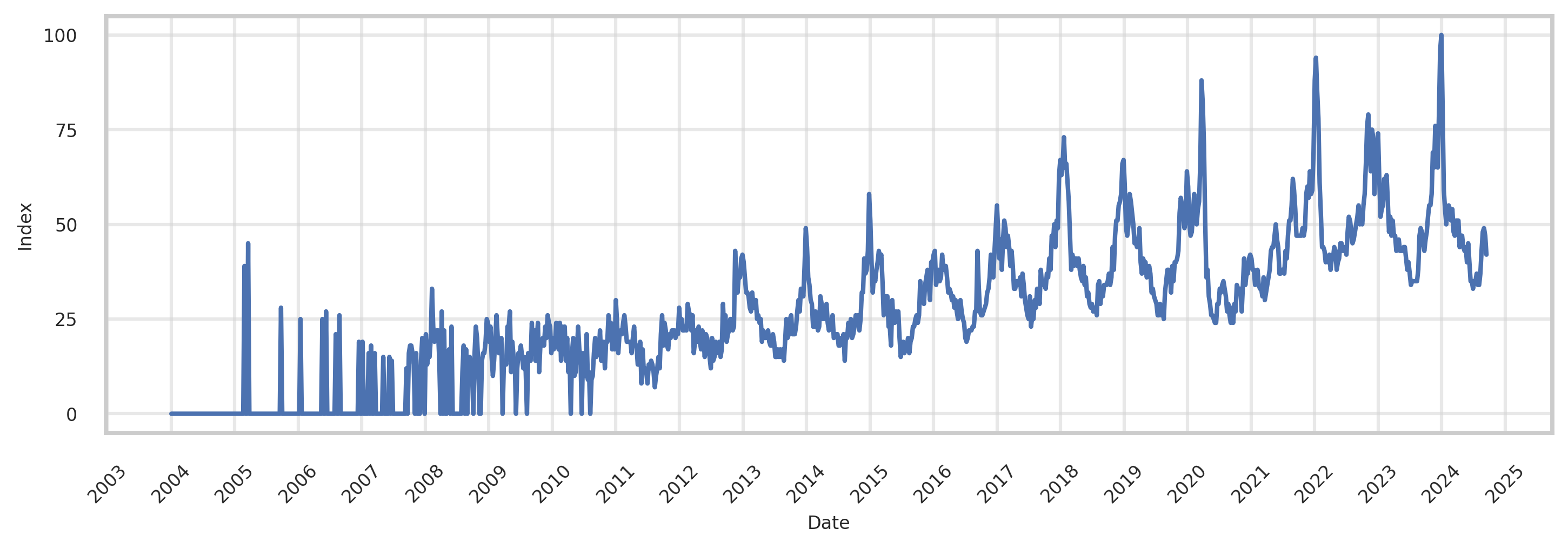
Figure 1: Example of search volumes over time for “Cough” in Alabama

To further explore relevant search activity, the “related queries” and “related topics” functionalities help us identify a broader set of terms and topics connected to the initial search keyword. They can be selected as “rising”, that is, emerging terms that had a significant increase in search volume, or “top”, that is, most popular search terms in the period, location and category chosen (Trends Help 2025b). Hence, choosing different time periods, regions or categories will give different related searches. Section 2.3 provides a more detailed approach to obtaining relevant keywords.

Google Trends provides real-time data that offers up-to-date information on search trends. This includes partial data retrieval during ongoing periods, such as the middle of the day, week or month, which is valuable for real-time forecasting. For example, the start of the week for weekly search volumes is Sunday, which allows to obtain partial volumes on Wednesday for the first four days of the week.

On the software development side, there are different ways to retrieve Google Trends search volumes. A csv file can be downloaded directly from the website. There exist R and Python packages (gtrendsR and pytrends) for convenient download. Google Trends contains an Application Programming Interface, which gives identical results to the Google Trends publicly available site but automates the process of downloading the data. For this paper, all our methods are applicable to direct downloads of search volumes from https://trends.google.com/trends/.

2.2 Challenges of Google Trends Data

The data generation mechanism in Google Trends introduces issues such as missing values, sampling variability, noise, and trends, that can affect forecasting quality. Figure 2 illustrates these challenges using search volumes for four different terms.

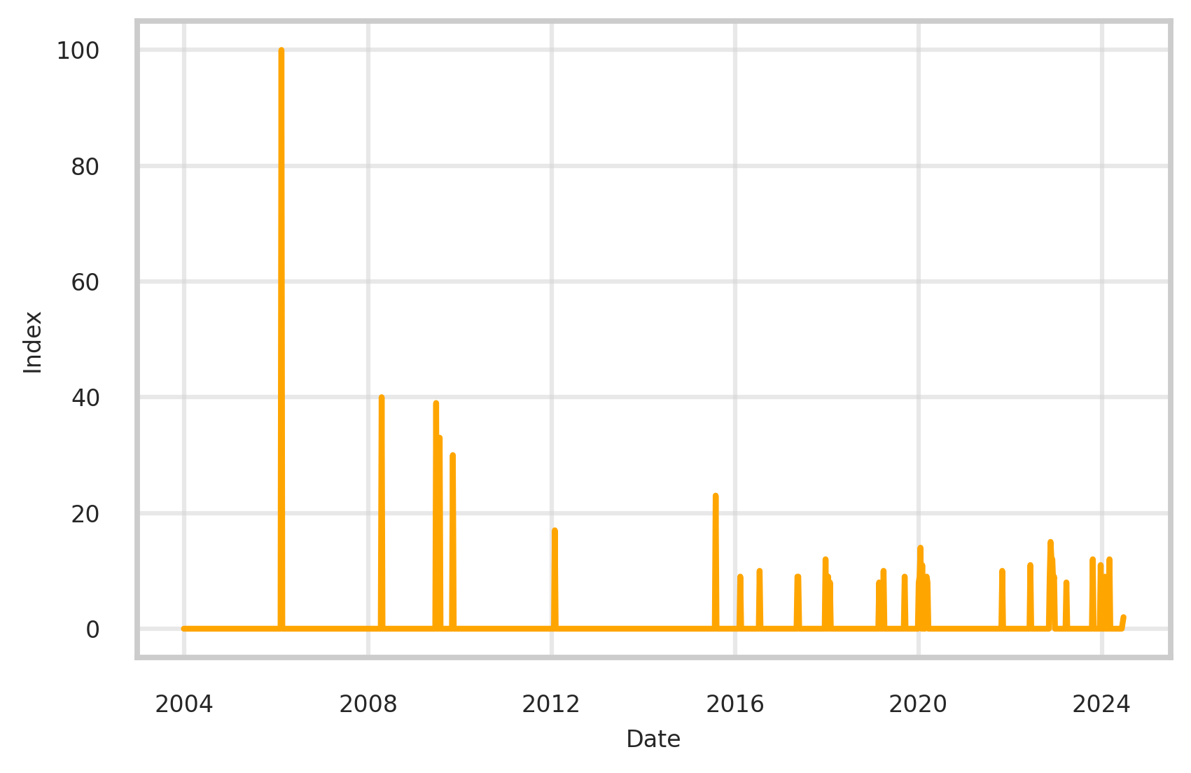
(a) Missing Values in “Influenza Treatment”

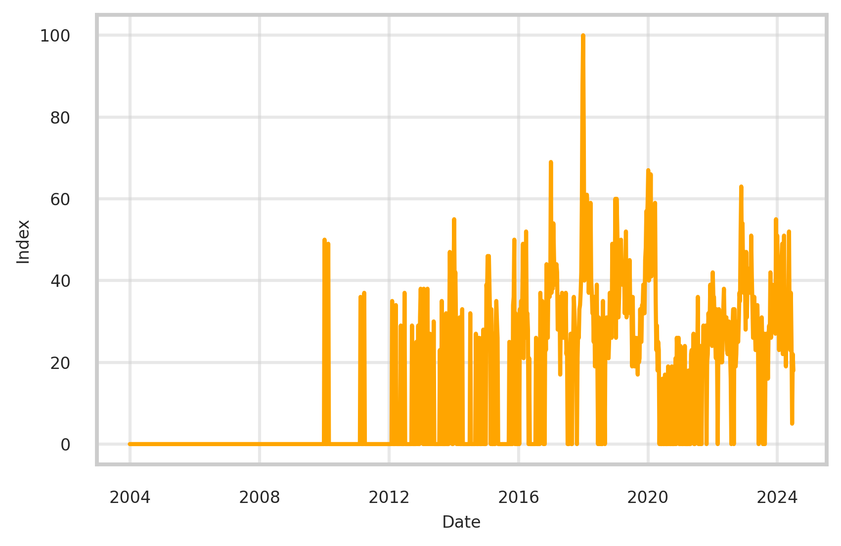
(b) Noise in “Acute Bronchitis”

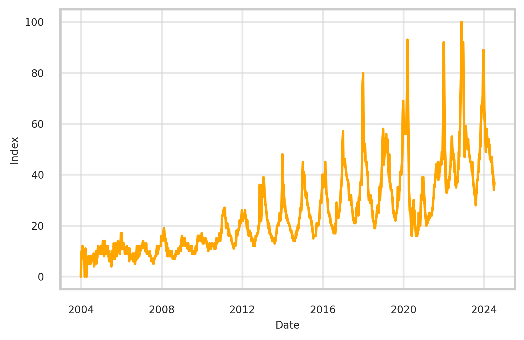
(c) Trend in “Cough”

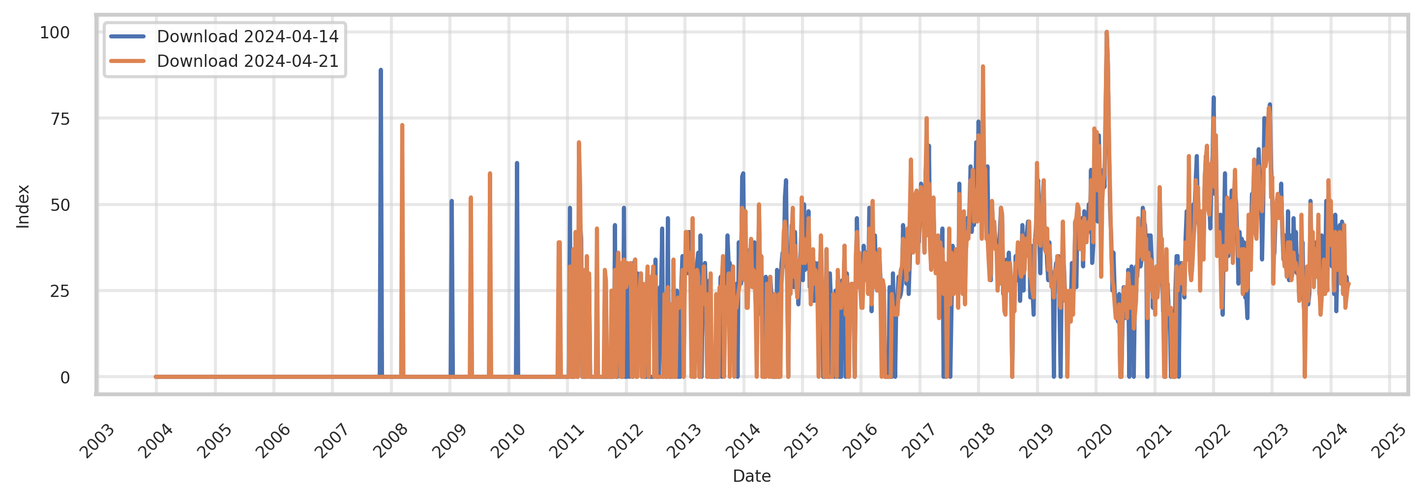
(d) Sampling Variability across different downloads for “Common Cold”

Figure 2: Examples of issues in Google Trends search volumes for California and Alaska

Google Trends assigns a value of “0” when the number of searches for a specific keyword falls below undisclosed privacy thresholds defined by Google, as illustrated in Figure 2(a). It indicates low search activity rather than a complete absence of searches. This can result in sparse data, particularly at the state or city level and for daily or weekly frequencies (Stephens-Davidowitz & Varian 2014). These zeros represent missing data that need to be addressed, as they mask low but potentially meaningful search activity.

Noise, shown in Figure 2(b), is also inherent in the data generation process of Google Trends. Given the billions of Google searches conducted daily, Google Trends provides only a representative sample to ensure quick response times (Trends Help 2025a). This sample is a random approximation of the entire population of searches, and thus contains sampling noise. To optimize processing, Google servers cache data for 24 hours, meaning that repeated input searches within the same day yield identical results. However, at midnight UTC, the cache resets, and a new sample is drawn, leading to day-to-day variability across different downloads of search volumes for the same search (Choi & Varian 2012, Neumann et al. 2023), as illustrated in Figure 2(d). This variability arises from the randomness of the sampling-based data generation process, which follows a hypergeometric distribution (Bleher & Dimpfl 2022). Let $K$ and $k$ be the search volumes for a keyword in a population of size $N$ and a sample of size $n$, respectively. Since $K$ and $N$ are unobserved, the reported proportion $\frac{k}{n}$ is a noisy approximation of $\frac{K}{N}$. Google Trends scales search volumes from 0 to 100, effectively returning $100\times\frac{k}{n}/\frac{K}{N}$. As $K$ decreases, the variance of $\frac{k}{n}/\frac{K}{N}$, which reflects sampling variability, increases. This leads to noisier estimates, especially for small regions and infrequent searches.

As terms become more or less popular with rising or declining public interest, search volumes may exhibit a trend, as displayed in Figure 2(c). It corresponds to a gradual change in the data over time, which can mask underlying patterns. In the context of Google Trends, this phenomenon can have multiple causes, including changes in vocabulary with new or obsolete terms, more or less general interest in a subject, or algorithm updates.

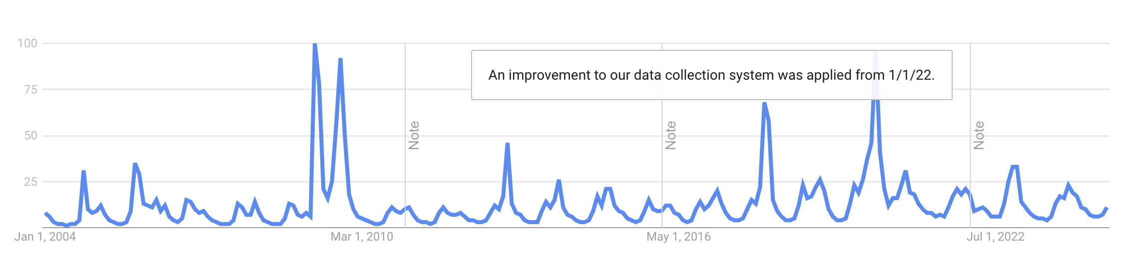
Figure S1: Google Trends website (accessed 2024-09-13) showing the “interest over time” for the search term “flu” from 2004 to 2024. The website includes annotations indicating data collection updates.

In fact, data quality could change as Google Trends’ algorithm undergoes updates. Cebrián & Domenech (2024) mention that there has been notable changes in Google Trends’ algorithms over the years. According to the Google Trends website, improvements to geographical assignment and data collection systems were implemented in 2011, 2016, and 2022, as shown in SI Figure S1. These updates can lead to inconsistencies. For example, Myburgh (2022) reports that changes to Google’s sampling strategy in January 2022 resulted in higher search volumes compared to earlier data. Consequently, data after January 2022 is not directly comparable to prior periods. Therefore, long-term trends may reflect algorithmic changes rather than genuine shifts in search behavior, posing challenges for accurate forecasting.

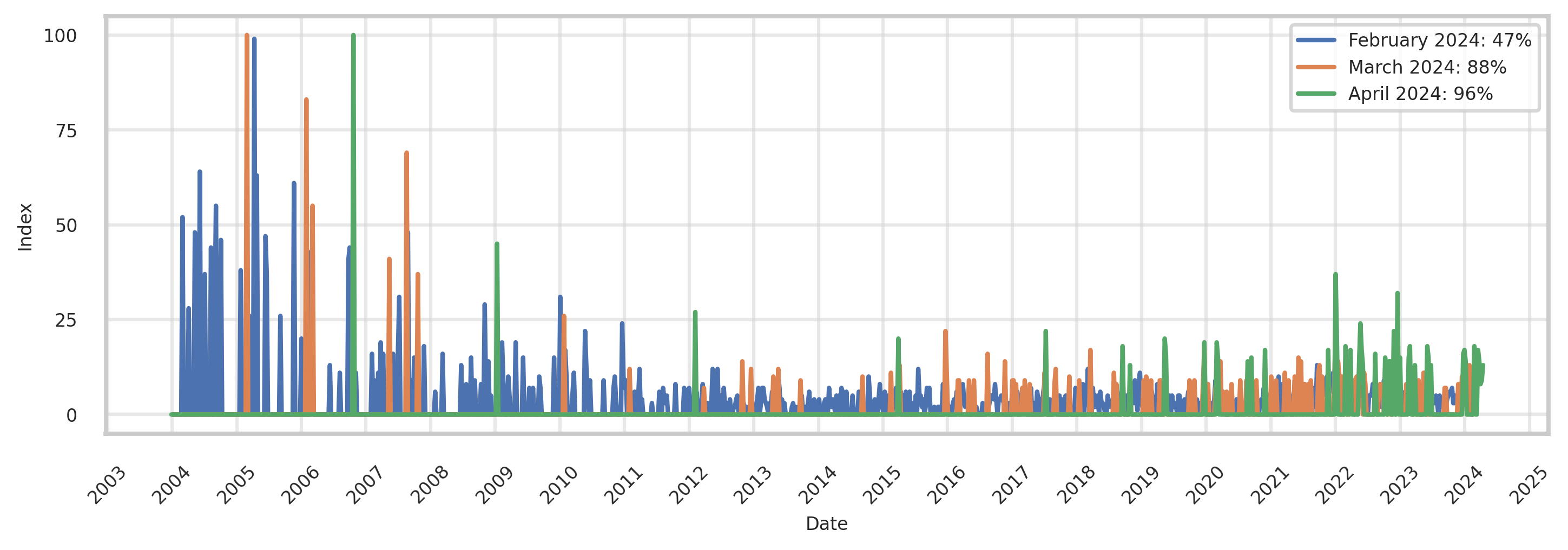
Figure 3: Example of changes in the percentage of zeros within different downloads of “Nasal Congestion” in Alaska from February to April 2024

We have also observed changes in Google Trends data within our dataset, where the total number of zeros increased by 40% at the start of 2024 (See SI Table S1). Figure 3 shows a 104% increase in the proportion of zeros for keyword “Nasal Congestion” between February and April 2024. This increase may be linked to another algorithm update, as the elevated number of zeros has been constant since. Therefore, it is critical to construct a preprocessing strategy that can handle updates from the data collection system.

2.3 Identifying Flu-related Terms from Google Trends

In this study, we analyze weekly Google Trends’ “interest over time” data for the United States at both national and state levels since 2004. Our initial set of 161 flu-related terms and topics is based on the work of Yang et al. (2015), identified through Google Correlate in 2009 and 2010, but the service was discontinued in 2019. Therefore, to expand our pool of keywords, we retrieve queries related to “flu”. For long-term seasonal analysis, “top” queries are preferred over “rising” ones, as they exhibit more consistent search patterns in the given time frame. We choose the “Cold and Flu” category to limit results to the area of infectious diseases, and select the entire period from 2004 onward to exclude event-specific queries (e.g., “flu 2024”). Keywords are tailored to each state by setting the corresponding location, which also restricts results to English (or the predominant local language), as opposed to collecting worldwide data. In summary, category, time period, and location serve as filters to refine the dataset. This approach yields time series of weekly search volumes for approximately 500 terms per state, covering symptoms, treatments, medicine, or types of flu.

2.4 Influenza Hospitalizations from CDC

Every year since 2013, the US Centers for Disease Control and Prevention organizes a “Predict the Influenza Season Challenge”, also called “FluSight”, which asks participating teams to forecast weekly influenza-related metrics in real-time. Initially requiring forecasts of outpatient influenza-like-illness (ILI) rates, the target variable shifted in 2021 to flu-related hospitalizations up to 4 weeks in the future (Mathis et al. 2024, Centers for Disease Control and Prevention 2025a). Several prediction methods are employed, generally together in an ensemble model, including statistical models like ARIMA (Kandula & Shaman 2019, Meyer et al. 2025), machine learning models such as gradient boosting (Meyer et al. 2025, Ray et al. 2024), mechanistic models with compartments (Aawar & Srivastava 2022), deep learning models like neural networks (Aiken et al. 2021). We use the data from this challenge to retrospectively evaluate the performance of using preprocessed Google Trends search volumes in predictive models.

Reporting of hospitalization data became mandatory on February 2, 2022 (Mathis et al. 2024), and admission counts, collected at both national and state levels in the United States by the National Healthcare Safety Network (NHSN) (Centers for Disease Control and Prevention 2025d) are publicly available in the GitHub repository from CDC Epidemic Prediction Initiative (2025). Influenza-related hospitalization data is released weekly with a one-week delay, while Google Trends data is available in real time, offering a timely informational advantage. In this study, we leverage search data as exogenous variables to perform 1-week-ahead prediction of flu hospitalizations.

To extend the training period for modeling, we follow the methodology of Meyer et al. (2025) to augment the dataset using ILINet data (Centers for Disease Control and Prevention 2025c) and FluSurv-Net data (Centers for Disease Control and Prevention 2025b) with transfer learning. This augmentation provides a continuous time series of hospitalization data starting from 2012.

3 Methods

In this section, we present our methodology to handle missing values, sampling variability, noise, and trends in Google Trends’ search volumes using hierarchical clustering, smoothing splines, and detrending techniques.

3.1 Missing Values and Sampling Variability

Zeros in Google Trends data, due to low search volumes, represent missing values. Addressing this issue is essential, as even minimal search activity can contain valuable insights. A common approach is to discard affected terms, but it risks eliminating meaningful information. An alternative is to impute zeros, which can introduce errors, especially in time series with high sparsity, as there may not be enough information to produce accurate estimates. To overcome this issue, we implement a hybrid approach, by discarding terms with insufficient data (over 99% of zeros), using keywords with fewer than 30% of missing values as individual predictors, and combining the remaining queries whose aggregated search volumes exceed privacy thresholds. Moreover, since phrases can be searched in any word order, we remove duplicated terms (e.g. “cold and flu” and “flu and cold”) by computing pairwise correlations between time series, and discarding one of the two variables when their correlations are higher than 0.99.

Google Trends enables the use of Boolean logic, where the “+” operator is interpreted as “or”, to obtain the union of search activity for multiple terms. This results in higher overall volumes with fewer zeros. As categorizing terms using expert knowledge is impractical and lacks reproducibility, we use a data-driven approach to ensure a systematic grouping. We associate terms using hierarchical clustering based on correlations as a similarity metric, following Ning et al. (2024)’s recommendation.

Hierarchical clustering (Ward 1963) is a data analysis technique that creates a sequence of nested clusters based on a hierarchical structure (Maharaj et al. 2019). We use Ward’s method to determine how clusters are merged, as it minimizes the total within-cluster variance at each step. This approach produces spherical clusters of relatively similar sizes (Maharaj et al. 2019, Everitt et al. 2011), ensures clear separation, and is regarded as one of the most robust and effective methods for noisy data (Balcan et al. 2014). Clusters with high similarity are merged together in successive steps. In hierarchical clustering, smaller, closely related clusters can be combined into broader groups, while larger ones can be subdivided to enhance relevance and specificity.

The similarity metric used in our hierarchical clustering is correlation distance, which is defined as $(1-\text{correlation matrix})$. Since different phrasings of a query often produce similar search results, their search volumes tend to align as well. Correlation matches time series that share similar shapes and have synchronized peaks and troughs. It also enables sparse signals with relevant spikes to be grouped with more complete ones, provided their key patterns align. Clustering keywords based on correlations thus forms groups that not only share semantic meanings but also have combined search volumes that surpass Google’s privacy thresholds. This approach effectively addresses the challenge of zeros while preserving meaningful search activity.

To determine the optimal number of clusters for hierarchical clustering, we use the elbow method, which plots the within-cluster sum of squares (WCSS) against the number of clusters. WCSS, defined as $\sum_{i=1}^{k}\sum_{x\in C_{i}}|x-\mu_{i}|^{2}$, where $\mu_{i}$ is the average time series of cluster $C_{i}$, measures the sum of squared distances between each time series and its cluster center (Maharaj et al. 2019, Hastie et al. 2017). As the number of clusters increases, WCSS decreases, with the optimal point occurring at the “elbow,” where adding more clusters yields diminishing returns. At the elbow, clusters strike a balance between capturing meaningful patterns and maintaining a sufficient size to surpass Google’s privacy thresholds. If a single cluster remains disproportionately large compared to the others, we apply a second round of hierarchical clustering to further subdivide it. The categorized queries are then grouped using the Boolean “+” operator, and their combined search volumes are retrieved from Google Trends. We finalize the clusters after confirming they contain low percentages of zeros.

Clustering not only addresses missing values, but also sampling variability. Popular keywords with high search volumes exhibit consistent behavior across different samples, while less popular terms with sparse data are subject to higher sampling variability (Medeiros & Pires 2021). Grouping such queries into clusters increases search volumes, effectively reducing hypergeometric sampling randomness and improving data reliability.

3.2 Noise

Noise in Google Trends data arises from random sampling variations, which can obscure the underlying signal and lead to overfitting. While various statistical techniques can estimate the true signal, real-time forecasting requires smoothing time series using only past data to prevent information leakage, where data not available at the time of estimation is inadvertently included in the model (Joseph 2022, Borup & Schütte 2022). Exponential smoothing and moving averages rely on past values but may introduce phase shifting, while K-nearest neighbors, kernel smoothing, and LOESS require both past and future points. Polynomial regression risks overfitting or underfitting, an Fourier transforms and wavelets need the entire time series for frequency and time-frequency analysis (Shumway et al. 2006, Brockwell & Davis 2016). Such constraints make these methods unsuitable for real-time applications. To overcome these challenges, we apply smoothing splines iteratively within a rolling window of past values. This approach offers localized data fitting, relies exclusively on past observations, provides precise control over smoothing, and has been shown to effectively remove noise (Musial et al. 2011, Navarrete & Viswanath 2018).

Smoothing splines (Reinsch 1967) aim to minimize the function

$$\sum_{t=1}^{n}(x_{t}-f_{t})^{2}+\lambda\int(f^{\prime\prime}_{t})^{2}dt,$$ (1)

where $x_{t}$ are the observations, $f_{t}$ is the cubic spline, and $\lambda$ is the smoothing parameter controlling the degree of smoothness (Hastie et al. 2017, Shumway et al. 2006). Larger $\lambda$ values produce smoother time series but risk shrinking peaks and flattening the signal, while smaller values may retain excessive noise. To balance these effects and avoid over-smoothing, we restrict $\lambda$ to the range [0.1, 2].

We implement an iterative denoising process tailored for real-time settings, performing one-step-ahead predictions of Google Trends search volumes. The data is split into training and testing sets, with optimal $\lambda$ values for each keyword identified through a grid search on the training set, and the test set used for out-of-sample denoising. During training, we fit smoothing splines on a rolling window of recent observations, and the next data point outside the window is predicted. The window then advances by one observation, and the process is repeated across the training set. During testing, smoothing splines are applied similarly, but the last fitted observation within the rolling window, not the predicted one, is used as the denoised value. This approach prevents overfitting to recent trends and ensures smoother transitions. The window size is determined through visualizations and performance evaluations.

Optimal $\lambda$ parameters are selected by minimizing the Root Mean Squared Error (RMSE) between the one-step-ahead predictions and the raw values. RMSE captures peaks and large variations common in Google Trends data, which often exhibits sudden spikes in search volumes. By penalizing large differences, this metric ensures that smoothing preserves peak magnitudes without excessive flattening.

Denoising is applied only to time series with high noise levels, identified by evaluating the RMSE associated with the optimal $\lambda$. Higher RMSE values indicate that noise dominates the series, making it difficult for the model to produce accurate predictions. If the RMSE for a series exceeds a predefined threshold, determined through analysis of time series patterns, smoothing is necessary. This strategy allows us to selectively improve noisy series while avoiding unnecessary adjustments for cleaner ones.

3.3 Trend

Trends in Google Trends data arise from long-term changes in search volumes, often driven by shifts in public interest or algorithm updates. While most keywords have search volumes with a relatively stable mean over time, some exhibit persistent trends. However, for applications such as predicting infectious disease surges, unemployment rates, or stock prices, the focus is typically on short-term patterns. Long-term trends can obscure these dynamics and introduce noise into forecasting models. Furthermore, a time series with a trend is non-stationary, complicating the accurate estimation of autocorrelations between observations (Shumway et al. 2006) and potentially distorting variable relationships. We apply methods such as model fitting or differencing, to remove trends and restore stationarity. Having access to Google Trends data since 2004 provides an advantage, allowing for a clear estimation of the long-term trend.

Time series trends can be classified as either deterministic or stochastic. A deterministic trend is a fixed and predictable pattern over time, following a linear or quadratic shape, and can be removed through detrending to achieve stationarity. A stochastic trend, on the other hand, arises from the cumulative effect of past values and random shocks, and should be eliminated through differencing. To identify the presence and the type of trend in a time series, we apply the Augmented Dickey-Fuller (ADF) test (Dickey & Fuller 1979) to each search volume time series. The null hypothesis ($H_{0}$) states that the time series has a unit root and is non-stationary, while the alternative hypothesis ($H_{1}$) is that the time series is stationary, potentially around a deterministic trend (Joseph 2022). Since search volumes are strictly non-negative, their time series have a non-zero mean. The ADF test fits a regression model to the time series data, as follows (Valenzuela et al. 2019):

$$\Delta x_{t}=\mu+\alpha t+\beta t^{2}+\gamma x_{t-1}+\sum_{i=1}^{p-1}\phi_{i}\Delta x_{t-i}+\epsilon_{t},$$ (2)

where $x_{t}$ is a time series, $\Delta x_{t}=x_{t}-x_{t-1}$ is the first difference, $\mu$ is the mean, $\alpha$ and $\beta$ are coefficients for linear and quadratic time trends, $t$ is the time index, $\gamma$ determines stationarity, $p$ is the lag order, and $\epsilon_{t}$ is the error term.

The ADF test operates by estimating the regression equation (2) to evaluate stationarity and guide necessary transformations under different assumptions about the type of trend in the data. We test $H_{0}:\gamma=0$ against $H_{1}:\gamma<0$. We first assess whether the series is stationary around a constant, non-zero mean, under the assumption $\mu\neq 0,\alpha=0,\beta=0$. If $H_{0}$ is rejected under this assumption, no further transformation is necessary. If not, the series may contain a trend. Next, we test whether the series is stationary around a linear deterministic trend, under the assumption $\mu\neq 0,\alpha\neq 0,\beta=0$. If $H_{0}$ is rejected under this assumption, the series requires linear detrending. Otherwise, it may contain a quadratic or stochastic trend. Finally, we test whether the series is stationary around a quadratic deterministic trend under the assumption $\mu\neq 0,\alpha\neq 0,\beta\neq 0$. Rejection of $H_{0}$ under this assumption indicates the need for quadratic detrending. If all tests fail to reject $H_{0}$, the series exhibits a stochastic trend and requires differencing. We use the significance level of $\alpha=0.05$.

To perform detrending, we estimate deterministic trends using ordinary least squares (OLS) regression and subtract the fitted line from the data. A linear trend is estimated as $\hat{m}_{t}=\mu+\alpha t$, while a quadratic trend is modeled as $\hat{m}_{t}=\mu+\alpha t+\beta t^{2}$. We remove the trend from the data as $x_{t}-\hat{m}_{t}$. Differencing, used for stochastic trends, is computed as $\hat{x}_{t}=x_{t}-x_{t-1}$. To avoid look-ahead bias, we estimate trend parameters using only the training set and apply transformations to the entire time series. Only the test set is used for model evaluation.

4 Results

This section presents a modularized evaluation of each preprocessing step, including clustering, denoising, and detrending, applied to Google Trends flu-related keywords, and highlights their individual contributions to improving data quality.

4.1 Evaluation of Clustering

Hierarchical clustering is applied to all terms and topics in the candidate pool of 500 terms for each location to produce clusters of keywords with denser time series. We evaluate the clustering results by visualizing search volumes and analyzing the percentage of zeros.

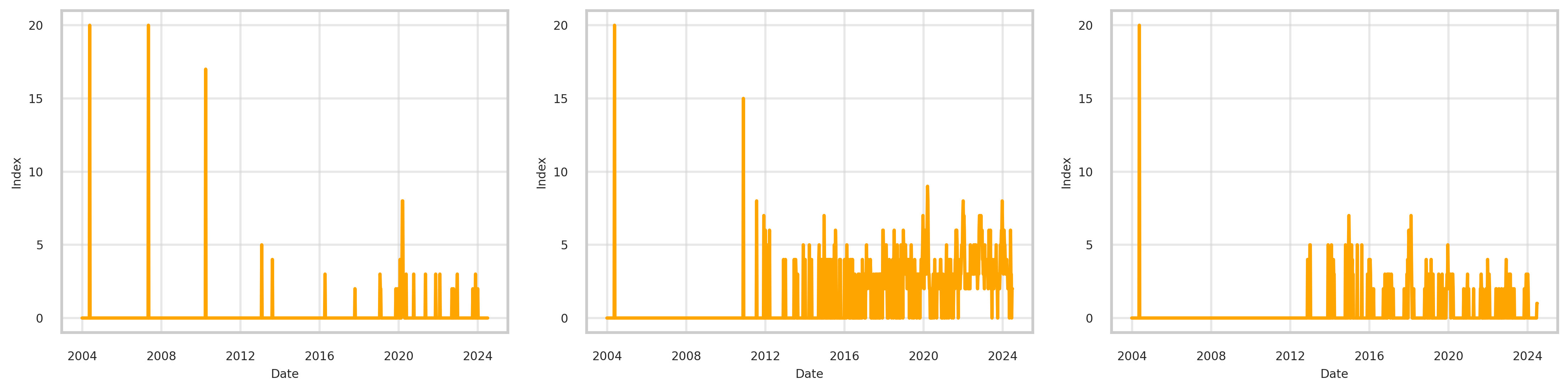
(a) Individual (large values truncated)

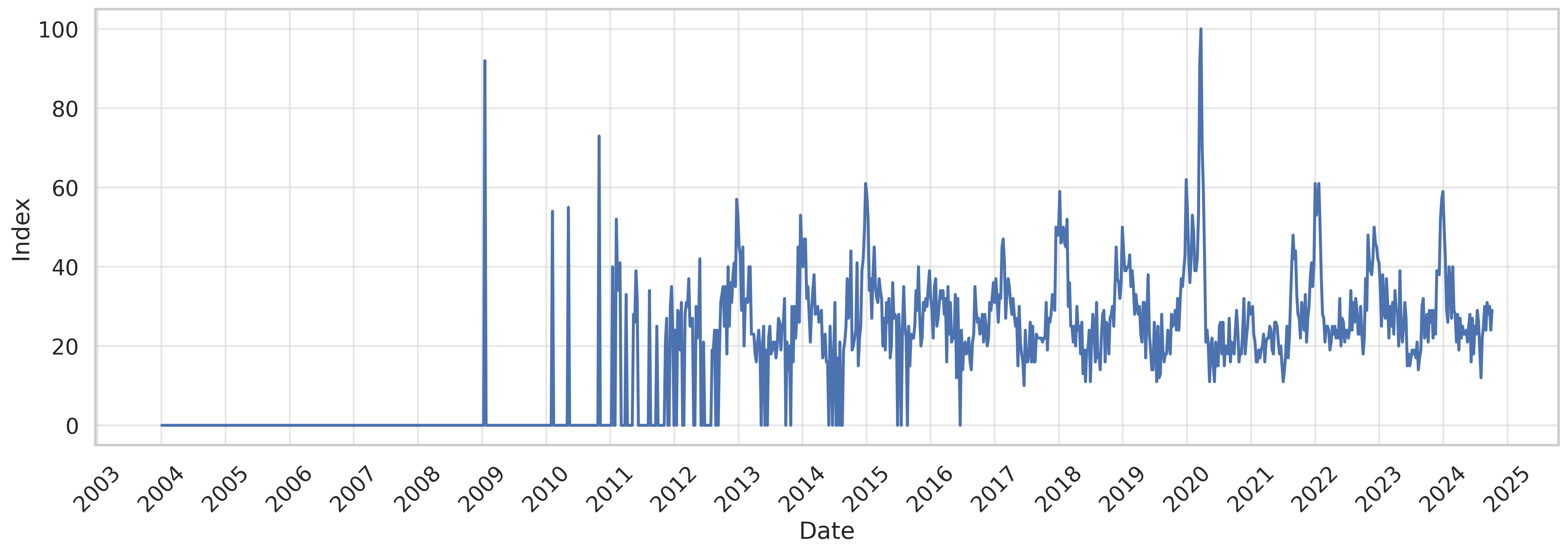
(b) Combined

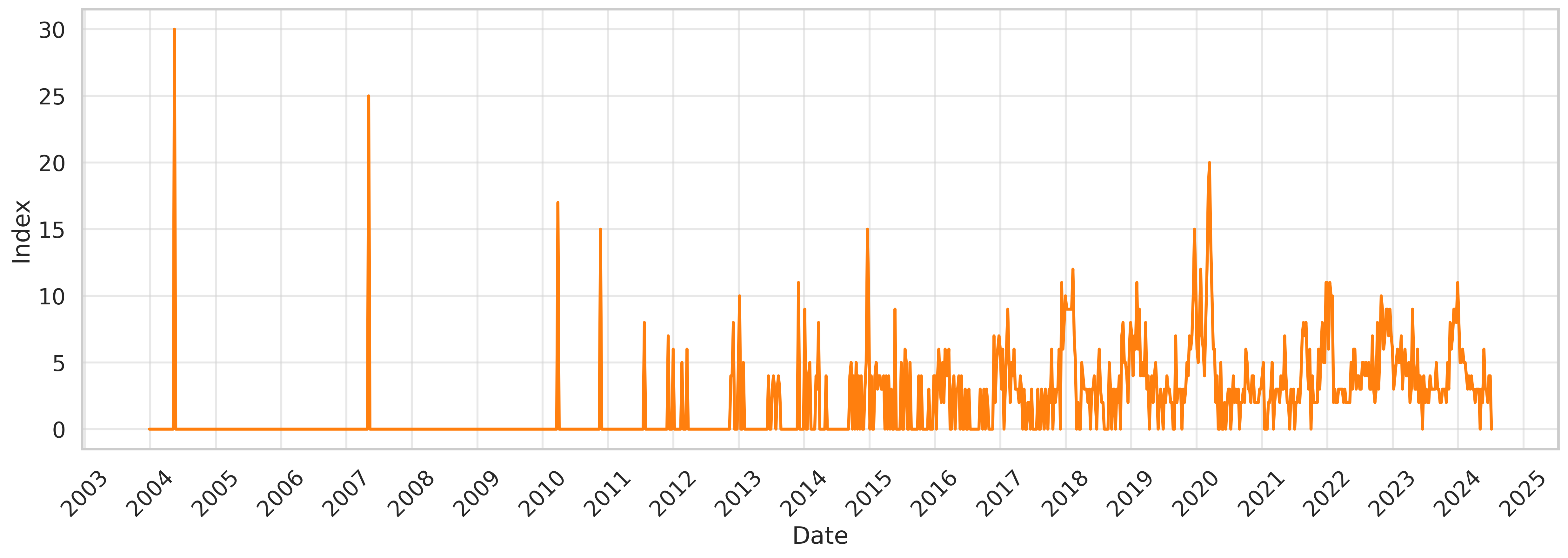
(c) Summation (large values truncated)

Figure 4: Example comparison of search volumes in Tennessee

Figure 4 compares the raw, combined and summed search volumes for an example cluster for Tennessee, composed of three keywords (“cold virus”, “high fever”, “symptoms of pneumonia”) whose individual time series displayed in Figure 4(a) have 96%, 63%, and 86% of zeros. Figure 4(b) reveals that their combined search volumes have a reduced percentage of zeros (40%) with clear and interpretable patterns. In contrast, simply summing the individual time series, as shown in Figure 4(c), results in 60% of zeros and less discernible patterns. This illustrates that clustering is an effective method for addressing data sparsity, as it generates usable time series by aggregating sparse keywords into meaningful groups.

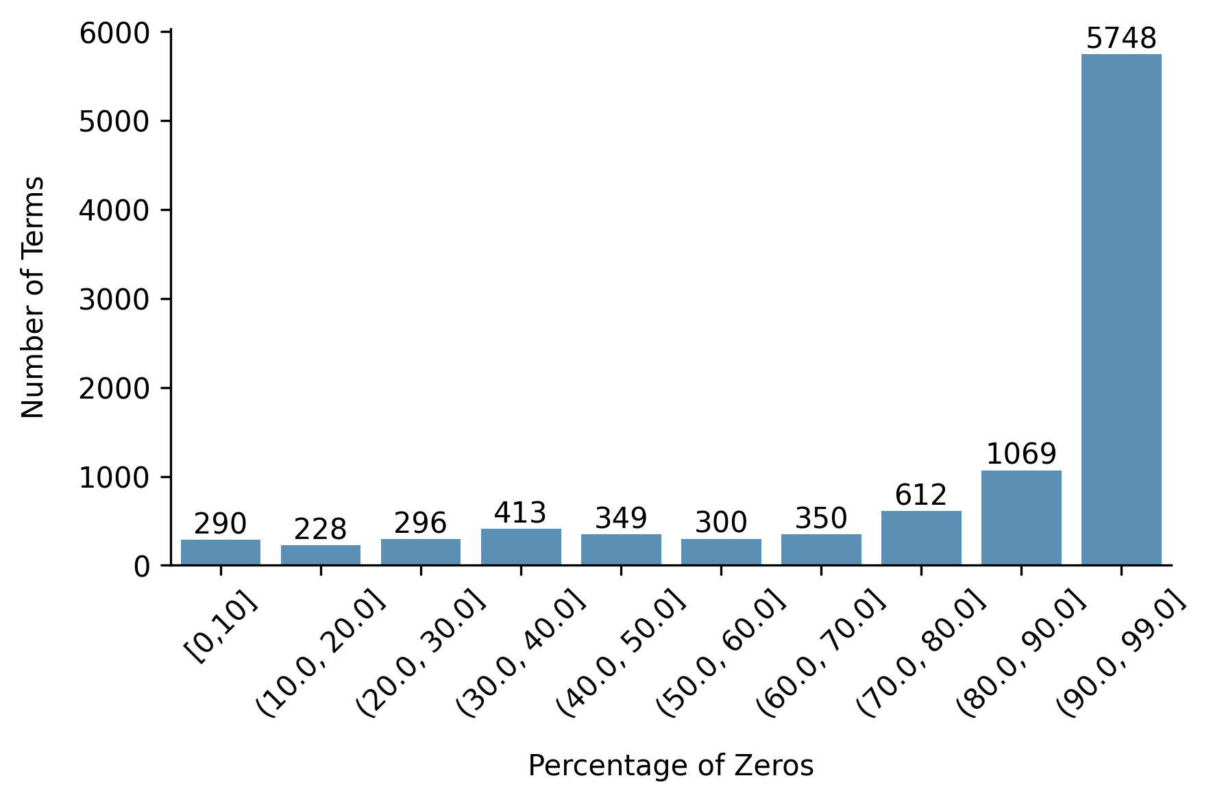
(a) Individual

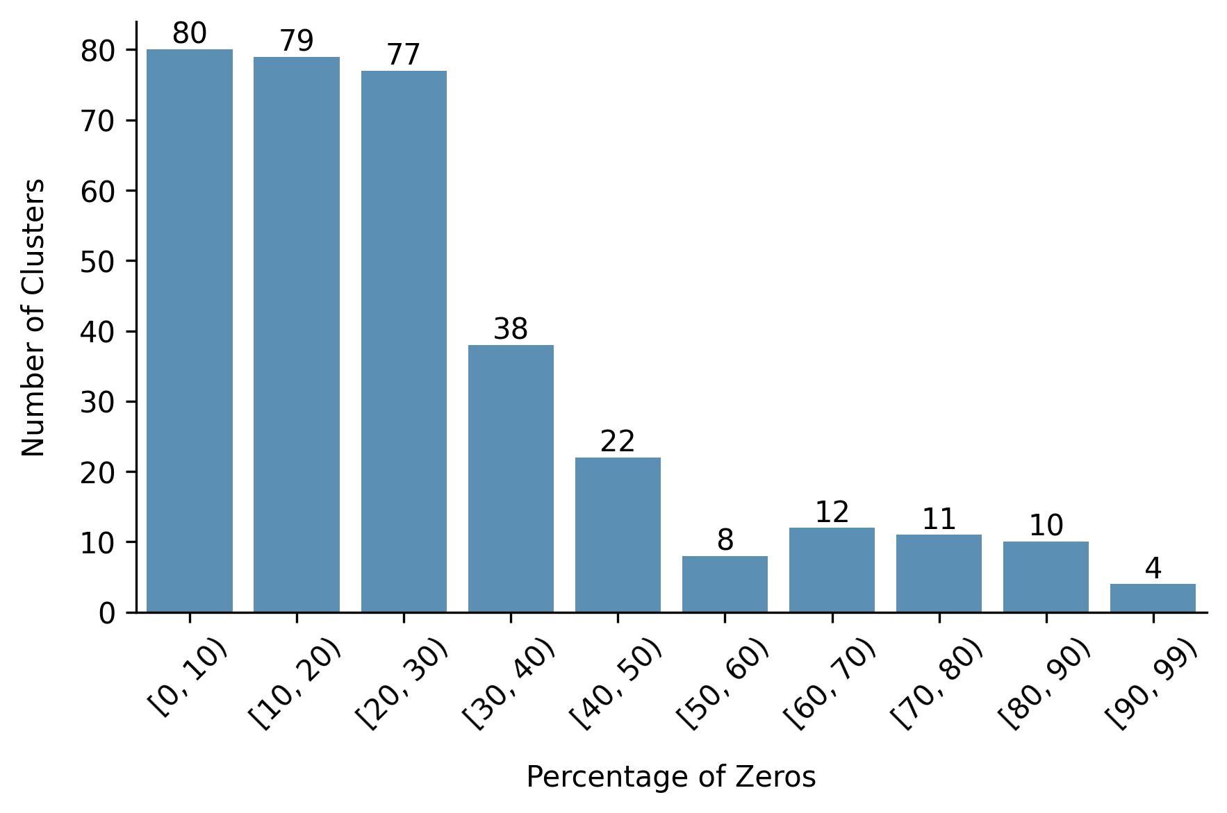
(b) Combined

Figure 5: Distribution of percentage of zeros in individual and combined search volumes across all locations

Figure 5 analyzes the percentage of missingness before and after clustering for all 28,580 keywords in our dataset. 814 queries with $\leq 30\%$ of zeros were retained in their original form, 8,841 with between 30% and 99% zeros were grouped into 341 clusters, and the remainder were discarded. Figure 5(a) shows that these individual search volumes often contain sparse data with many zeros. After clustering, the percentage of zeros in the aggregated search volumes is notably reduced, as shown in Figure 5(b). Most clusters fall within the [0–10]% range of zeros, with very few clusters in the [90–99]% range, demonstrating a substantial reduction in sparsity. Our method thus transforms sparse data dominated by zeros into denser aggregated data, improving signal quality.

4.2 Evaluation of Denoising

Among the 1,155 resulting clusters and individual keywords, smoothing splines are applied to 622 variables requiring denoising. We assess the effectiveness of our smoothing procedure by analyzing noise levels across various downloads retrieved over several months.

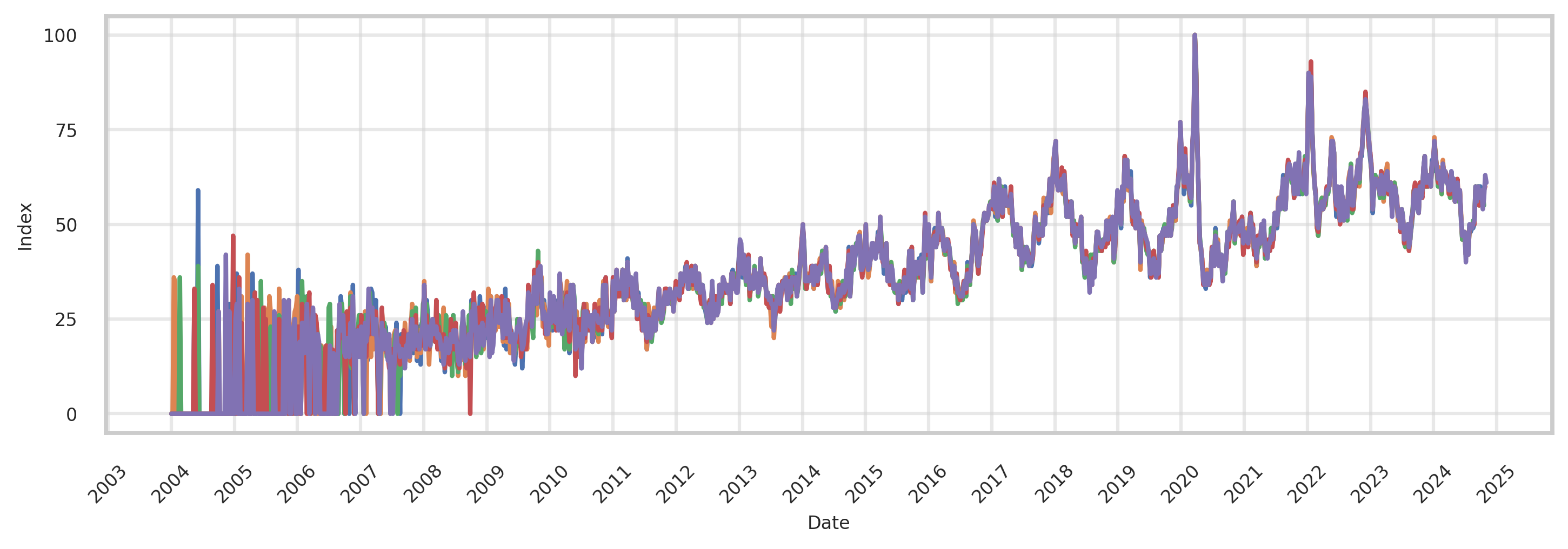
(a) Raw

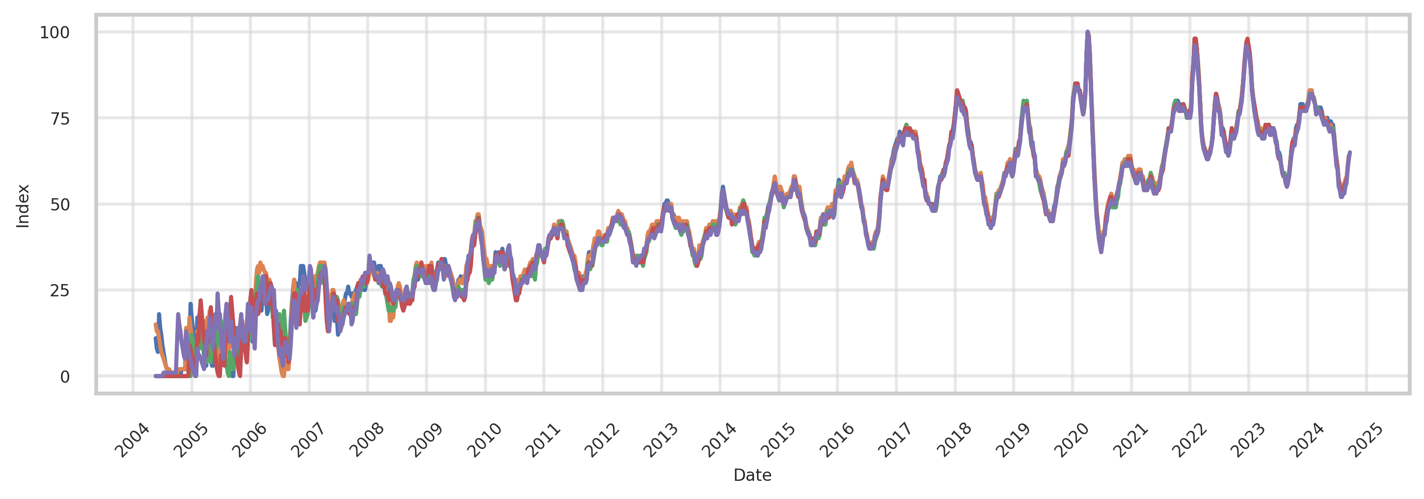
(b) Denoised

Figure 6: Example comparison of noise levels before and after denoising across five downloads in Alaska

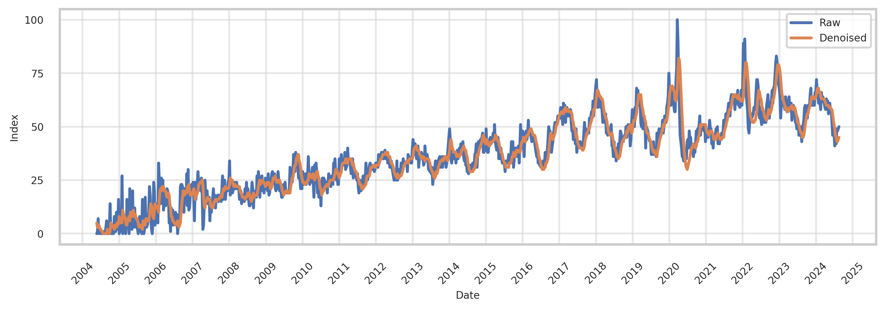
(a) Average

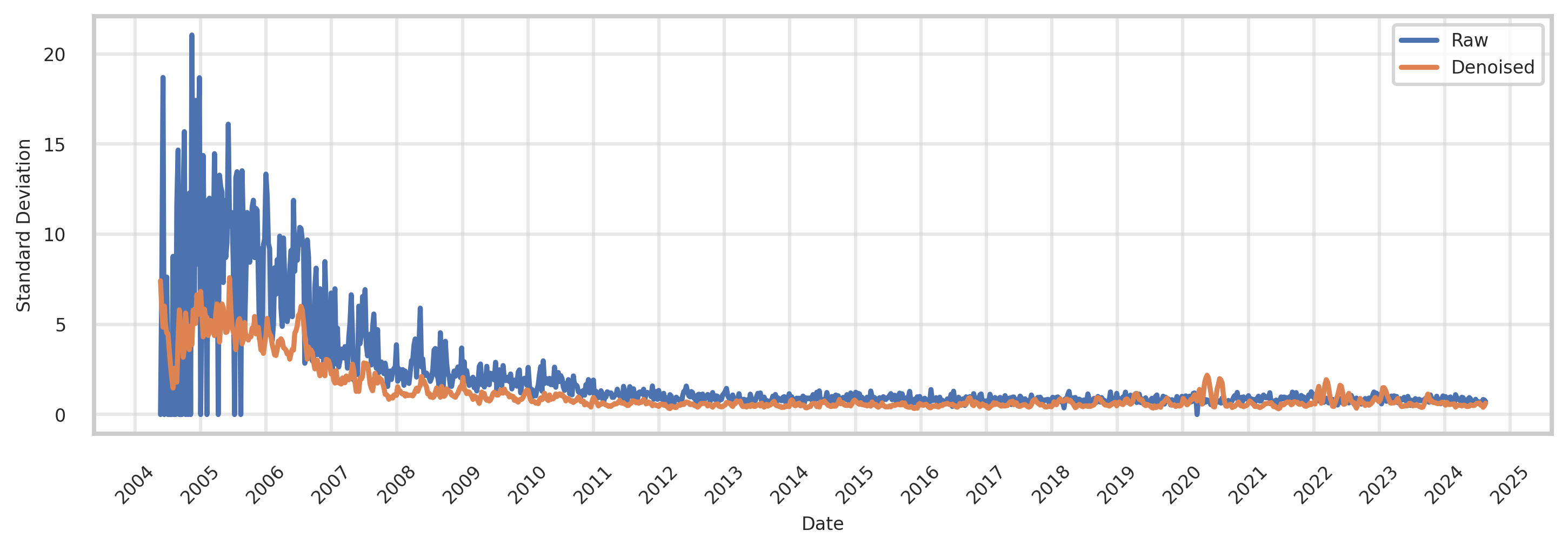
(b) Standard deviation

Figure 7: Descriptive statistics before and after denoising across 27 downloads in Alaska example

Figure 6 visualizes noise reduction before and after denoising across five repeated downloads for a cluster in Alaska. The raw data in Figure 6(a) exhibit substantial noise and sampling variability, while the denoised data in Figure 6(b) display much cleaner signals. Figure 7 depicts the averages and standard deviations of the series at each time step across twenty-seven downloads. The averages of raw and denoised data (Figure 7(a)) show similar peaks and troughs, meaning that the smoothing method preserves the overall signal structure and main trends. The lower standard deviation in the denoised data (Figure 7(b)) indicates that smoothing reduces sampling variability and noise, leading to a more stable signal.

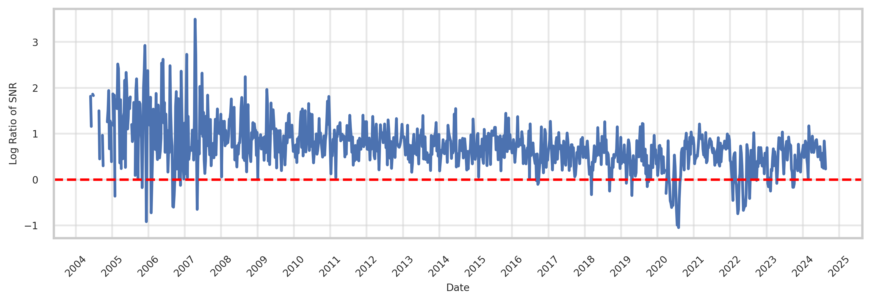
(a) Single keyword in Alaska example

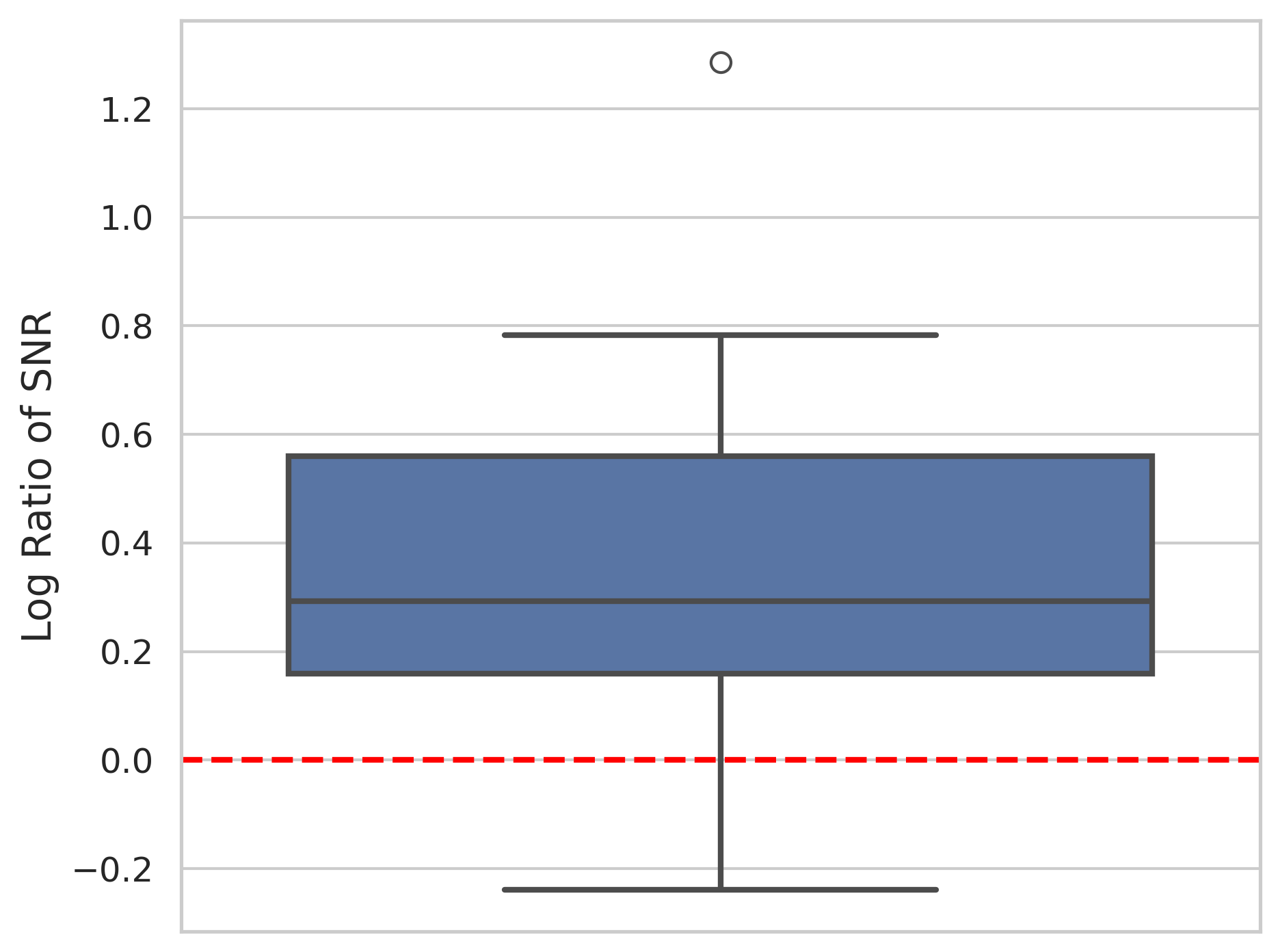
(b) Summary across all keywords and locations

Figure 8: Log ratio of SNR across 27 downloads. Higher is better.

Effective denoising should minimize short-term fluctuations while preserving underlying patterns. The Signal-to-Noise Ratio (SNR) measures the power of the signal to the power of the noise (Palani & Kalaiyarasi 2022). Since real-world data lacks a clear distinction between signal and noise, Smith et al. (1999) define SNR as the ratio of the mean to the standard deviation of the data, $\text{SNR}=\mu/\sigma$, where $\mu$ reflects the overall magnitude of the signal, and $\sigma$ approximates the noise level. A higher SNR indicates a cleaner signal. We estimate the SNR at each time step as $\hat{\mu}_{t}/\hat{\sigma}_{t}$, where $\hat{\mu}_{t}$ and $\hat{\sigma}_{t}$ are the mean and standard deviation of the time series at time $t$ across downloads. The log ratio of SNR between denoised and raw data is then computed as:

$$\text{log Ratio of SNR}=\log\left(\frac{\hat{\mu}_{t}^{\text{(denoised)}}}{\hat{\sigma}_{t}^{\text{(denoised)}}}\Big{/}\frac{\hat{\mu}_{t}^{\text{(raw)}}}{\hat{\sigma}_{t}^{\text{(raw)}}}\right).$$ (3)

Figure 8 presents the log ratio of SNR across twenty-seven downloads. Figure 8(a) illustrates its temporal evolution for a single time series, while Figure 8(b) displays the results across all keywords. Predominantly positive values indicate that denoised data have higher SNR than raw data, confirming that denoising enhances signal quality by reducing noise and sampling variability.

4.3 Evaluation of Detrending

Detrending is applied after denoising to keywords that exhibit a trend based on the ADF test. To assess its effectiveness in removing deterministic trends, we use the regression coefficient of determination ($R^{2}$), which quantifies how well the estimated trend explains the variability of the data. This metric is computed on the entire time series between the estimated trend and the data. A lower $R^{2}$ after detrending indicates successful trend removal.

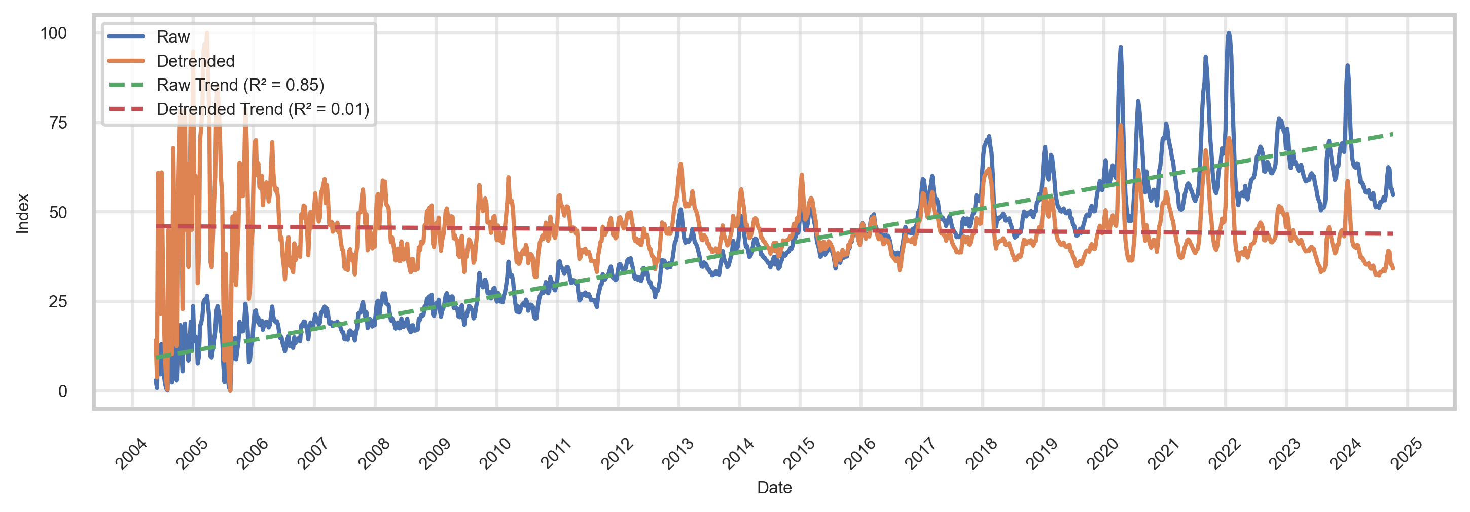
Figure 9: Example of estimated deterministic trend in raw and detrended data in Alabama

Figure 9 displays the time series of a cluster in Alabama before and after detrending, along with their respective fitted trends. Before detrending, $R^{2}$ equals 0.85, meaning the trend accounts for 85% of the variability. After detrending, it drops to 0.01, confirming that the trend no longer dominates the data.

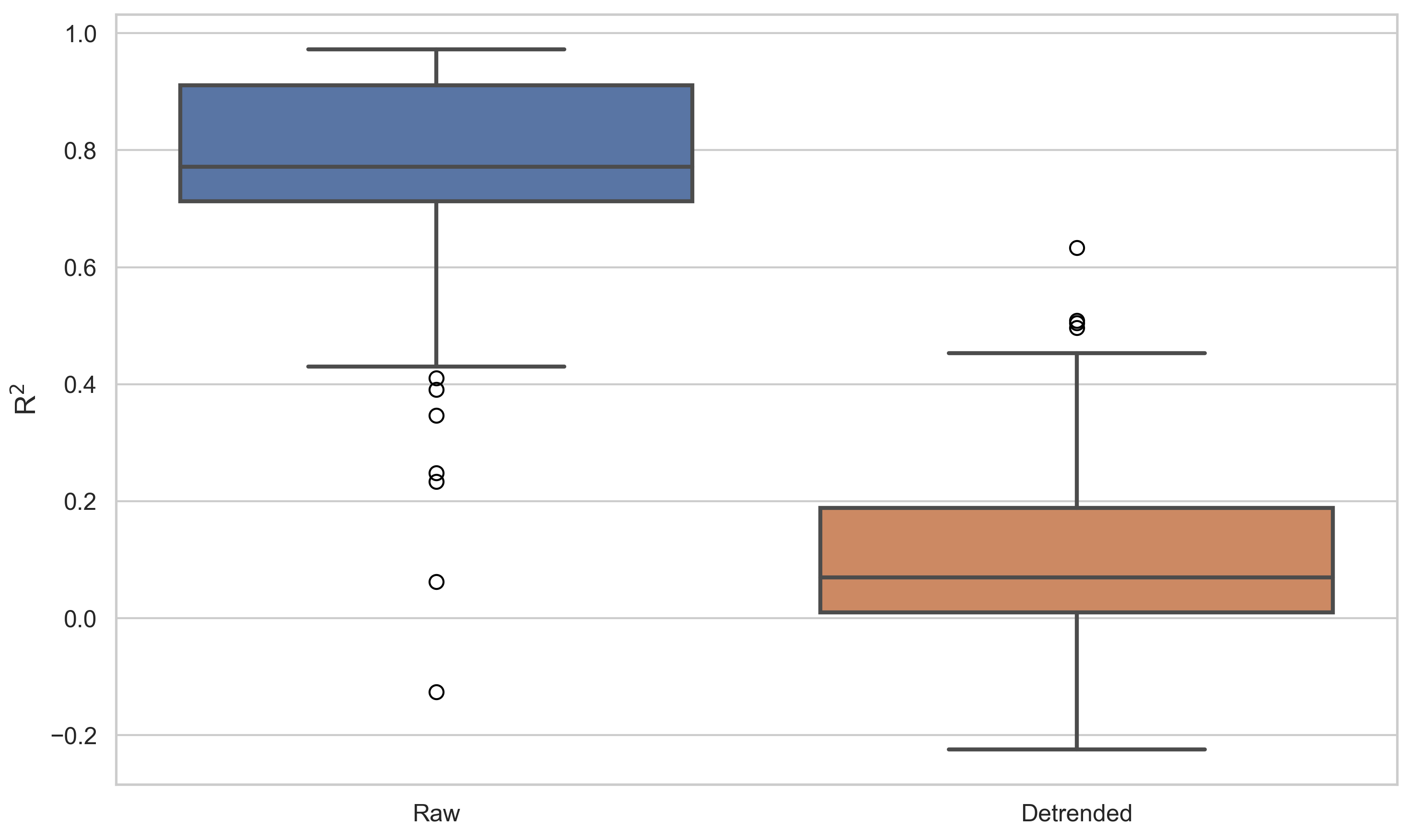
Figure 10: Summary of $R^{2}$ for deterministic trends before and after detrending across all locations

Figure 10 summarizes the distribution of $R^{2}$ across all keywords. Fitted trends in the raw data exhibit high $R^{2}$ values (mean $=0.77$), confirming that they were well estimated. After detrending, $R^{2}$ values decrease significantly (mean $=0.11$), demonstrating the effective removal of deterministic trends. There are a few outliers with low $R^{2}$ values before detrending and high values afterward, suggesting occasional misestimation, as stationarity is detected based on the training set and may not fully capture time series patterns.

5 Application to Influenza Prediction

To validate the effectiveness of our methodology, we use a univariate ARIMAX(1,1,1) model to compare the forecasting performance of our preprocessed Google Trends data with that of raw data in the context of real-time flu forecasting. ARIMA models are widely used for short-term predictions due to their ease of implementation, computational efficiency, and interpretability. In influenza forecasting, ARIMA has consistently demonstrated strong accuracy for 1-week-ahead predictions (Meyer et al. 2025, Mathis et al. 2024), making it a reliable baseline for evaluating more complex methods (Kandula & Shaman 2019). Studies have also shown that incorporating exogenous variables, such as Google Trends data, into autoregressive models significantly improves nowcasting performance (Lampos et al. 2015). Accordingly, we extend ARIMA with Google Trends data to evaluate the impact of our preprocessing approach on forecasting flu hospitalizations.

5.1 ARIMAX as a Predictive Model

AutoRegressive Integrated Moving Average with eXogenous variables (ARIMAX) (Tiao & Box 1981) is an extension of the ARIMA model (Box & Jenkins 1970) that incorporates external predictors. Let $y_{t}$ be the target variable and $x_{t,k}$ the $k^{\text{th}}$ exogenous variable at time $t$. The model used in this study is a univariate ARIMAX(1,1,1) with first-order differencing, expressed as:

$$\Delta y_{t}=\mu+\phi_{1}\Delta y_{t-1}+\theta_{1}\epsilon_{t-1}+\epsilon_{t}+\sum_{k=1}^{K}\beta_{k}x_{t,k}.$$ (4)

Here, $\Delta y_{t}$ denotes the differenced target series, $\mu$ is the mean of the differenced series, $\phi_{1}$ and $\theta_{1}$ represent the coefficients for the autoregressive (AR) and moving average (MA) terms, respectively, and $\epsilon_{t}$ is the current error term. The coefficients $\beta_{k}$ correspond to the exogenous variables (Peixeiro 2022). Readers unfamiliar with the general ARIMA model are referred to Supporting Information Section § B.

Model (4) is applied to each location for retrospective out-of-sample 1-week-ahead forecasts to simulate real-time predictions. This approach allows for comparing forecasting performance across three scenarios: using preprocessed Google Trends data, non-preprocessed data, and no exogenous variables. The model is trained on a rolling window of 104 weeks, with optimal parameters determined by minimizing the training loss, calculated as the sum of squared fitting errors within each training window. After each forecast, the rolling window shifts forward by one week, and the model is retrained to predict the following week’s target. To assess forecasting performance, we calculate the Mean Squared Error (MSE) between the ground truth and predicted values, $\text{MSE}=\frac{1}{T}\sum_{t=1}^{T}(y_{t}-\hat{y}_{t})^{2}$, over the test period $t=1,...,T$. We then compute the Relative Efficiency (RE) as the ratio of MSEs between two models. The overall RE is based on the average MSE across all $n$ states as $\frac{\sum_{i=1}^{n}\text{MSE}_{i}\text{(ARIMAX(1,1,1))}}{\sum_{i=1}^{n}\text{MSE}_{i}\text{(ARIMA(1,1,1))}}$ (Ning et al. 2019), where ARIMA(1,1,1) without exogenous variables serves as the benchmark.

The pool of keywords is obtained through Google Trends’ “related queries”, which may include terms lacking semantic relevance that cannot be manually excluded. The raw non-preprocessed dataset of individual queries is very large, while the dataset of preprocessed data is much smaller as queries are combined. To identify meaningful predictors, we calculate their correlations with the target variable and select those within the top 25th percentile for preprocessed data and 98th percentile for raw data for each state, with a maximum of 35 predictors per state. This state-specific threshold ensures that states with weaker correlations retain at least a few predictors, while states with stronger correlations include only the most relevant keywords. To prevent multicollinearity, we remove one of any pair of variables whose correlation exceeds 0.90. Correlations are computed exclusively on the training set to prevent look-ahead bias and preserve the integrity of the real-time forecasting framework.

5.2 Results

We retrospectively evaluate our approach using flu hospitalization data at both national and state (including DC) levels in the United States over the past two seasons, from October 17, 2022, to April 27, 2024. The training set extends up to October 2022. This serves as an end-to-end validation of our preprocessing pipeline, demonstrating its practical utility in real-world forecasting scenarios.

Method	National	State
Clustering + Denoising + Detrending (Preprocessed)	0.42	0.76
Clustering + Denoising	0.45	0.79
Clustering	0.51	0.90
Non-Preprocessed	1.54	1.22

Table 1: Relative Efficiency and Ablation Study at the US national and state levels

Table 1 displays the relative efficiencies of ARIMAX models at the US national and state levels, comparing different levels of preprocessing of exogenous variables. Since a lower MSE indicates better forecasting performance, a relative efficiency below 1 signifies an improvement over the benchmark ARIMA(1,1,1) model. Our results show that preprocessing Google Trends data enhances prediction accuracy, reducing error by 58% at the national level (RE = 0.42) and by an average of 24% at the state level (RE = 0.76). In contrast, using raw, non-preprocessed data deteriorates performance, increasing prediction error by 54% at the national level and 22% at the state level. These findings highlight the important role of preprocessing in improving predictive accuracy.

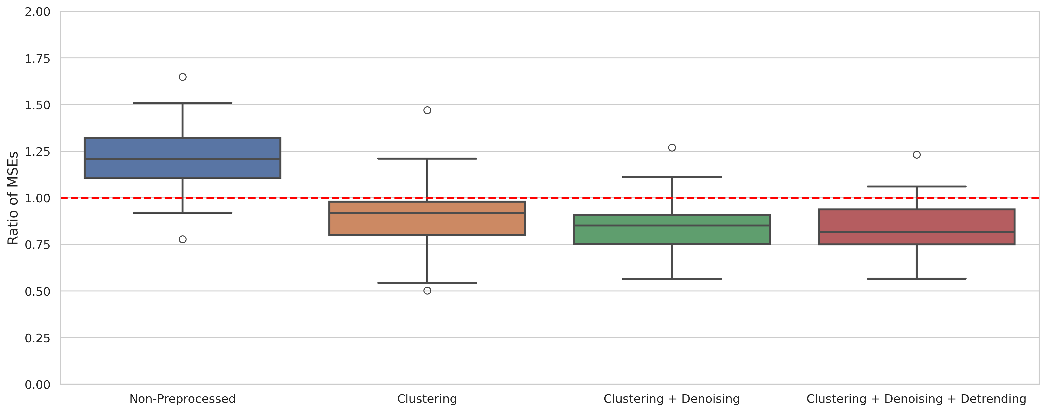
Figure 11: Summary of ratio of MSEs across all states (large outliers hidden). Lower is better.

Figure 11 extends the analysis presented in Table 1 by exploring the RE at the state level. For 88% of the states, incorporating preprocessed Google Trends data enhances model accuracy, as evidenced by the majority of the boxplot falling below 1. In contrast, the first boxplot reveals that using raw explanatory variables generally worsens performance, with only four locations showing any benefiting from unprocessed data.

We compare the forecast errors of the benchmark ARIMA model and ARIMAX with fully preprocessed variables at both national and state levels using statistical significance tests. These ensure that the observed improvements are statistically meaningful and unlikely to be due to random chance. First, we apply Student’s one-sided paired t-test (Student 1908) to test the equality of mean errors between ARIMA and ARIMAX, against the alternative hypothesis that ARIMA produces smaller errors than ARIMAX. This test is conducted on the combined data from all states, with 80 observations per location across 51 locations, resulting in a total of 4,080 observations. The overall p-value for the state-level data is $3.17\times 10^{-6}$ with a t-value of $-4.52$, well below the 0.05 significance threshold, strongly supporting rejection of the null hypothesis. This indicates that ARIMAX significantly reduces forecast error compared to ARIMA, confirming the benefit of incorporating preprocessed exogenous variables. At the national level, however, the p-value is 0.37 with a t-value of $-0.37$, showing no significant difference in the mean errors between ARIMA and ARIMAX.

To further assess forecast accuracy at the national level, we perform the Diebold-Mariano (DM) test (Diebold & Mariano 1995), a widely used method to evaluate forecast accuracy (D’Amuri & Marcucci 2017, Bantis et al. 2023). We incorporate modifications from Harvey et al. (1997), which enhance robustness in small samples, as our analysis includes only 80 observed forecast errors per location. The null hypothesis of the DM test states that two competing models have the same predictive accuracy over time. The test yields a p-value of 0.044 and a t-value of 1.73, suggesting that ARIMAX provides more stable predictive performance over time compared to ARIMA, even though it does not exhibit significantly lower average errors. The results from both tests demonstrate that the proposed end-to-end preprocessing methodology significantly improves forecasting accuracy.

6 Discussion and Conclusion

In this paper, we investigate the data generation mechanism of Google Trends and propose a comprehensive statistical preprocessing methodology to maximize its utility for forecasting. Our approach integrates hierarchical clustering to address missing values and sampling variability, dynamic smoothing splines to reduce noise, and detrending to separate short-term signals from long-term trends. Each preprocessing step is independently evaluated to validate its effectiveness in improving search data quality. We further demonstrate the practical benefits of our approach through an application to flu hospitalization prediction, showing improved accuracy when incorporating preprocessed search data into a statistical predictive model.

While our method has proven effective, it is not without limitations. First, keyword selection relied on Google Trends’ “related queries” feature, which occasionally included terms unrelated to flu. Rather than manually excluding these terms, we mitigated their impact through clustering, which reduces the influence of a single irrelevant term on the aggregated search volumes, and by applying a correlation filter to exclude terms with low relevance to the target variable. Second, the clustering process occasionally grouped semantically unrelated terms, but these clusters remained meaningful in terms of their time series patterns, ensuring their utility in prediction. Third, the quality of Google Trends data varies significantly across locations, with lower internet penetration resulting in inherently poor data quality that preprocessing techniques cannot fully address. Finally, we intentionally chose a simple univariate ARIMAX model to evaluate the effectiveness of our preprocessing techniques. While more complex statistical and machine learning models could produce higher forecasting accuracy, they might obscure the direct contributions of Google Trends data. Using an interpretable model aligns with the primary focus of this paper, which is to evaluate and substantiate the effectiveness of our preprocessing methodology, rather than to develop a flu hospitalization prediction model.

Future research could investigate the generalizability of our preprocessing methodology under different conditions, expanding on this study’s focus on enhancing Google Trends data quality for flu hospitalization prediction in the United States. A natural extension would be to apply our approach to other locations, where variations in search behavior, vocabulary, historical trends, and data availability may impact performance. Differences in internet penetration and regional interest could result in varying levels of missing data or noisier patterns, requiring adjustments in preprocessing. Similarly, our methodology could be tested on other infectious diseases or even non-health-related forecasting tasks, as long as search data remains a relevant predictor of the target. Identifying meaningful search terms may be more challenging in domains where prior knowledge is limited, unlike influenza, where symptoms and seasonal patterns are well understood. Moreover, other search-based data sources beyond Google Trends, such as those from search engines, social media platforms, or AI-driven tools, could provide additional signals for forecasting. Understanding how these alternative data sources differ in terms of missing values, sampling variability, noise, and trends, and whether they require similar preprocessing strategies, would help establish the robustness and stability of our methodology across a wider range of applications.

Acknowledgments

Supporting Information

Appendix A Google Trends

Date	Percentage
2024-02-11	64%
2024-02-25	84%
2024-03-10	84%
2024-03-24	84%
2024-04-07	86%
2024-04-21	87%

Table S1: Overall percentage of zeros across multiple downloads of Google Trends search volumes for the same 161 keywords across 52 locations.

Appendix B General ARIMA$(p,d,q)$ Model

An AutoRegressive Integrated Moving Average $\text{ARIMA}(p,d,q)$ model is used to forecast time series data. It is defined by three components, autoregression (AR), differencing (I), and moving average (MA), specified by parameters $p$, $d$ and $q$. The AR part indicates that a current value of the time series depends on $p$ of its past (or lagged) observations, while the MA part indicates it is a linear combination of $q$ of its lagged forecast errors. The I component specifies how many times ($d$) the time series is differenced to make it stationary, to stabilize the mean and variance.

The general ARIMA($p,d,q$) model can be written as [46]:

$$\Delta^{d}y_{t}=\mu+\sum_{i=1}^{p}\phi_{i}\Delta^{d}y_{t-i}+\sum_{i=1}^{q}\theta_{i}\epsilon_{t-i}+\epsilon_{t}.$$

The first operation $\Delta^{d}y_{t}=y_{t}-\sum_{i=1}^{d}d_{i}y_{t-i}$ represents the $d$-order differencing of the target series $y_{t}$ to achieve stationarity, with $d_{i}$ as the binomial coefficients corresponding to various orders of differencing. $\mu$ is the mean of the differenced series, $\phi_{i}$ are the coefficients for the $p$-order AR terms, which depend on past values of the differenced series $\Delta^{d}y_{t-i}$. $\theta_{i}$ are the coefficients for the $q$-order MA terms, involving past error terms $\epsilon_{t-i}$. $\epsilon_{t}$ is the current error term, assumed to follow a white noise process.

The ARIMA model is widely used for time series analysis due to its ability to model stationary and non-stationary data effectively. By integrating exogenous variables, the ARIMAX extension allows for incorporating external predictors, such as Google Trends data, to improve forecasting performance.

References

- [1]
- Aawar & Srivastava [2022] Aawar, M. A. & Srivastava, A. [2022], ‘Random forest of epidemiological models for influenza forecasting’, arXiv preprint arXiv:2206.08967 .
- Aiken et al. [2021] Aiken, E. L., Nguyen, A. T., Viboud, C. & Santillana, M. [2021], ‘Toward the use of neural networks for influenza prediction at multiple spatial resolutions’, Science Advances 7(25), eabb1237.
- Balcan et al. [2014] Balcan, M.-F., Liang, Y. & Gupta, P. [2014], ‘Robust hierarchical clustering’, The Journal of Machine Learning Research 15(1), 3831–3871.
- Bantis et al. [2023] Bantis, E., Clements, M. P. & Urquhart, A. [2023], ‘Forecasting gdp growth rates in the united states and brazil using google trends’, International Journal of Forecasting 39(4), 1909–1924.
- Bleher & Dimpfl [2022] Bleher, J. & Dimpfl, T. [2022], ‘Knitting multi-annual high-frequency google trends to predict inflation and consumption.’, Econometrics and Statistics 24, 1–26.
- Borup & Schütte [2022] Borup, D. & Schütte, E. C. M. [2022], ‘In search of a job: Forecasting employment growth using google trends’, Journal of Business & Economic Statistics 40(1), 186–200.
- Box & Jenkins [1970] Box, G. E. & Jenkins, G. M. [1970], Time series analysis: forecasting and control, Holden-Day.
- Brockwell & Davis [2016] Brockwell, P. J. & Davis, R. A. [2016], Introduction to time series and forecasting, 3rd edn, Springer.
- CDC Epidemic Prediction Initiative [2025] CDC Epidemic Prediction Initiative [2025], ‘Flusight forecast hub’, https://github.com/cdcepi/FluSight-forecast-hub. Accessed: 2025-02-10.
- Cebrián & Domenech [2023] Cebrián, E. & Domenech, J. [2023], ‘Is google trends a quality data source?’, Applied Economics Letters 30(6), 811–815.
- Cebrián & Domenech [2024] Cebrián, E. & Domenech, J. [2024], ‘Addressing google trends inconsistencies’, Technological Forecasting and Social Change 202, 123318.
- Centers for Disease Control and Prevention [2025a] Centers for Disease Control and Prevention [2025a], ‘About flu forecasting’, https://www.cdc.gov/flu-forecasting/about/index.html. Accessed: 2025-02-10.
- Centers for Disease Control and Prevention [2025b] Centers for Disease Control and Prevention [2025b], ‘Fluview: Laboratory-confirmed influenza hospitalizations’, https://gis.cdc.gov/GRASP/Fluview/FluHospRates.html. Accessed: 2025-02-10.
- Centers for Disease Control and Prevention [2025c] Centers for Disease Control and Prevention [2025c], ‘Fluview: National, regional, and state level outpatient illness and viral surveillance’, https://gis.cdc.gov/grasp/fluview/fluportaldashboard.html. Accessed: 2025-02-10.
- Centers for Disease Control and Prevention [2025d] Centers for Disease Control and Prevention [2025d], ‘Hospital respiratory data’, https://www.cdc.gov/nhsn/psc/hospital-respiratory-reporting.html. Accessed: 2025-02-10.
- Choi & Varian [2012] Choi, H. & Varian, H. [2012], ‘Predicting the present with google trends’, Economic record 88, 2–9.
- Dickey & Fuller [1979] Dickey, D. A. & Fuller, W. A. [1979], ‘Distribution of the estimators for autoregressive time series with a unit root’, Journal of the American statistical association 74(366a), 427–431.
- Diebold & Mariano [1995] Diebold, F. X. & Mariano, R. S. [1995], ‘Comparing predictive accuracy’, Journal of Business & Economic Statistics 20(1), 134–144.
- D’Amuri & Marcucci [2017] D’Amuri, F. & Marcucci, J. [2017], ‘The predictive power of google searches in forecasting us unemployment’, International Journal of Forecasting 33(4), 801–816.
- Eichenauer et al. [2022] Eichenauer, V. Z., Indergand, R., Martínez, I. Z. & Sax, C. [2022], ‘Obtaining consistent time series from google trends’, Economic Inquiry 60(2), 694–705.
- Everitt et al. [2011] Everitt, B., Landau, S., Leese, M. & Stahl, D. [2011], Cluster Analysis, 5th edn, John Wiley & Sons, Ltd.
- Fenga [2020] Fenga, L. [2020], ‘Filtering and prediction of noisy and unstable signals: The case of google trends data’, Journal of Forecasting 39(2), 281–295.
- Ginsberg et al. [2009] Ginsberg, J., Mohebbi, M. H., Patel, R. S., Brammer, L., Smolinski, M. S. & Brilliant, L. [2009], ‘Detecting influenza epidemics using search engine query data’, Nature 457(7232), 1012–1014.
- Google News Initiative [2025] Google News Initiative [2025], ‘Basics of google trends’, https://newsinitiative.withgoogle.com/resources/trainings/google-trends/basics-of-google-trends/. Accessed: 2025-02-10.
- Harvey et al. [1997] Harvey, D., Leybourne, S. & Newbold, P. [1997], ‘Testing the equality of prediction mean squared errors’, International Journal of forecasting 13(2), 281–291.
- Hastie et al. [2017] Hastie, T., Tibshirani, R. & Friedman, J. [2017], The elements of statistical learning: data mining, inference, and prediction, 2nd edn, Springer.
- Joseph [2022] Joseph, M. [2022], Modern Time Series Forecasting with Python: Explore industry-ready time series forecasting using modern machine learning and deep learning, Packt Publishing Ltd.
- Kandula et al. [2019] Kandula, S., Pei, S. & Shaman, J. [2019], ‘Improved forecasts of influenza-associated hospitalization rates with google search trends’, Journal of the Royal Society Interface 16(155), 20190080.
- Kandula & Shaman [2019] Kandula, S. & Shaman, J. [2019], ‘Near-term forecasts of influenza-like illness: An evaluation of autoregressive time series approaches’, Epidemics 27, 41–51.
- Lampos et al. [2021] Lampos, V., Majumder, M. S., Yom-Tov, E., Edelstein, M., Moura, S., Hamada, Y., Rangaka, M. X., McKendry, R. A. & Cox, I. J. [2021], ‘Tracking covid-19 using online search’, NPJ digital medicine 4(1), 17.
- Lampos et al. [2015] Lampos, V., Miller, A. C., Crossan, S. & Stefansen, C. [2015], ‘Advances in nowcasting influenza-like illness rates using search query logs’, Scientific reports 5(1), 12760.
- Liu et al. [2015] Liu, Y., Chen, Y., Wu, S., Peng, G. & Lv, B. [2015], ‘Composite leading search index: a preprocessing method of internet search data for stock trends prediction’, Annals of Operations Research 234, 77–94.
- Maharaj et al. [2019] Maharaj, E. A., D’Urso, P. & Caiado, J. [2019], Time series clustering and classification, Chapman and Hall/CRC.
- Mathis et al. [2024] Mathis, S. M., Webber, A. E., León, T. M., Murray, E. L., Sun, M., White, L. A., Brooks, L. C., Green, A., Hu, A. J., Rosenfeld, R. et al. [2024], ‘Evaluation of flusight influenza forecasting in the 2021–22 and 2022–23 seasons with a new target laboratory-confirmed influenza hospitalizations’, Nature communications 15(1), 6289.
- Matsa et al. [2017] Matsa, K. E., Mitchell, A. & Stocking, G. [2017], ‘The flint water crisis: Methodology’, https://www.pewresearch.org/journalism/2017/04/27/google-flint-methodology/. Pew Research Center Journalism & Media [Internet].
- Medeiros & Pires [2021] Medeiros, M. C. & Pires, H. F. [2021], ‘The proper use of google trends in forecasting models’, arXiv preprint arXiv:2104.03065 .
- Meyer et al. [2025] Meyer, A. G., Lu, F., Clemente, L. & Santillana, M. [2025], ‘A prospective real-time transfer learning approach to estimate influenza hospitalizations with limited data’, Epidemics p. 100816.
- Musial et al. [2011] Musial, J. P., Verstraete, M. M. & Gobron, N. [2011], ‘Comparing the effectiveness of recent algorithms to fill and smooth incomplete and noisy time series’, Atmospheric chemistry and physics 11(15), 7905–7923.
- Myburgh [2022] Myburgh, P. H. [2022], ‘Infodemiologists beware: recent changes to the google health trends api result in incomparable data as of 1 january 2022’, International Journal of Environmental Research and Public Health 19(22), 15396.
- Navarrete & Viswanath [2018] Navarrete, R. & Viswanath, D. [2018], ‘Prediction of dynamical time series using kernel based regression and smooth splines’.
- Neumann et al. [2023] Neumann, K., Mason, S. M., Farkas, K., Santaularia, N. J., Ahern, J. & Riddell, C. A. [2023], ‘Harnessing google health trends data for epidemiologic research’, American journal of epidemiology 192(3), 430–437.
- Ning et al. [2024] Ning, S., Hussain, A. & Wang, Q. [2024], ‘Incorporating connectivity among internet search data for enhanced influenza-like illness tracking’, PloS one 19(8), e0305579.
- Ning et al. [2019] Ning, S., Yang, S. & Kou, S. [2019], ‘Accurate regional influenza epidemics tracking using internet search data’, Scientific reports 9(1), 5238.
- Palani & Kalaiyarasi [2022] Palani, S. & Kalaiyarasi, D. [2022], Principles of digital signal processing, Springer.
- Peixeiro [2022] Peixeiro, M. [2022], Time series forecasting in python, Simon and Schuster.
- Preis et al. [2013] Preis, T., Moat, H. S. & Stanley, H. E. [2013], ‘Quantifying trading behavior in financial markets using google trends’, Scientific reports 3(1), 1–6.
- Rabiolo et al. [2021] Rabiolo, A., Alladio, E., Morales, E., McNaught, A. I., Bandello, F., Afifi, A. A. & Marchese, A. [2021], ‘Forecasting the covid-19 epidemic by integrating symptom search behavior into predictive models: Infoveillance study’, Journal of medical Internet research 23(8), e28876.
- Ray et al. [2024] Ray, E. L., Wang, Y., Wolfinger, R. D. & Reich, N. G. [2024], ‘Flusion: Integrating multiple data sources for accurate influenza predictions’, arXiv preprint arXiv:2407.19054 .
- Reinsch [1967] Reinsch, C. H. [1967], ‘Smoothing by spline functions’, Numerische mathematik 10(3), 177–183.
- Santillana et al. [2014] Santillana, M., Zhang, D. W., Althouse, B. M. & Ayers, J. W. [2014], ‘What can digital disease detection learn from (an external revision to) google flu trends?’, American journal of preventive medicine 47(3), 341–347.
- Shumway et al. [2006] Shumway, R. H., Stoffer, D. S. & Stoffer, D. S. [2006], Time series analysis and its applications with R examples, 2nd edn, Springer.
- Silva et al. [2019] Silva, E. S., Hassani, H., Madsen, D. Ø. & Gee, L. [2019], ‘Googling fashion: forecasting fashion consumer behaviour using google trends’, Social Sciences 8(4), 111.
- Smith et al. [1999] Smith, S. W. et al. [1999], The scientist and engineer’s guide to digital signal processing, 2nd edn, California Technical Pub.
- Stephens-Davidowitz [2017] Stephens-Davidowitz, S. [2017], Everybody lies: What the internet can tell us about who we really are, Bloomsbury Publishing.
- Stephens-Davidowitz & Varian [2014] Stephens-Davidowitz, S. & Varian, H. [2014], ‘A hands-on guide to google data’, further details on the construction can be found on the Google Trends page .
- Student [1908] Student [1908], ‘The probable error of a mean’, Biometrika pp. 1–25.
- Tiao & Box [1981] Tiao, G. C. & Box, G. E. [1981], ‘Modeling multiple time series with applications’, journal of the American Statistical Association 76(376), 802–816.
- Trends Help [2025a] Trends Help [2025a], ‘Faq about google trends data’, https://support.google.com/trends/answer/4365533?hl=en. Accessed: 2025-02-10.
- Trends Help [2025b] Trends Help [2025b], ‘Find related searches’, https://support.google.com/trends/answer/4355000?hl=en&ref_topic=4365530. Accessed: 2025-02-10.
- Trends Help [2025c] Trends Help [2025c], ‘Refine trends results by category’, https://support.google.com/trends/answer/4359597?hl=en. Accessed: 2025-02-10.
- Trends Help [2025d] Trends Help [2025d], ‘Search tips for trends’, https://support.google.com/trends/answer/4359582?hl=en. Accessed: 2025-02-10.
- Valenzuela et al. [2019] Valenzuela, O., Rojas, F., Pomares, H. & Rojas, I. [2019], Theory and Applications of Time Series Analysis, Springer.
- Wang et al. [2022] Wang, T., Ma, S., Baek, S. & Yang, S. [2022], ‘Covid-19 hospitalizations forecasts using internet search data’, Scientific Reports 12(1), 9661.
- Ward [1963] Ward, J. H. [1963], ‘Hierarchical grouping to optimize an objective function’, Journal of the American statistical association 58(301), 236–244.
- Yang et al. [2021] Yang, S., Ning, S. & Kou, S. [2021], ‘Use internet search data to accurately track state level influenza epidemics’, Scientific reports 11(1), 4023.
- Yang et al. [2017] Yang, S., Santillana, M., Brownstein, J. S., Gray, J., Richardson, S. & Kou, S. [2017], ‘Using electronic health records and internet search information for accurate influenza forecasting’, BMC infectious diseases 17, 1–9.
- Yang et al. [2015] Yang, S., Santillana, M. & Kou, S. C. [2015], ‘Accurate estimation of influenza epidemics using google search data via argo’, Proceedings of the National Academy of Sciences 112(47), 14473–14478.