FAME: Introducing Fuzzy Additive Models for Explainable AI

Abstract

In this study, we introduce the Fuzzy Additive Model (FAM) and FAM with Explainability (FAME) as a solution for Explainable Artificial Intelligence (XAI). The family consists of three layers: (1) a Projection Layer that compresses the input space, (2) a Fuzzy Layer built upon Single Input-Single Output Fuzzy Logic Systems (SFLS), where SFLS functions as subnetworks within an additive index model, and (3) an Aggregation Layer. This architecture integrates the interpretability of SFLS, which uses human-understandable if-then rules, with the explainability of input-output relationships, leveraging the additive model structure. Furthermore, using SFLS inherently addresses issues such as the curse of dimensionality and rule explosion. To further improve interpretability, we propose a method for sculpting antecedent space within FAM, transforming it into FAME. We show that FAME captures the input-output relationships with fewer active rules, thus improving clarity. To learn the FAM family, we present a deep learning framework. Through the presented comparative results, we demonstrate the promising potential of FAME in reducing model complexity while retaining interpretability, positioning it as a valuable tool for XAI.

I Introduction

Deep Learning (DL) has become essential across various applications, yet it faces transparency challenges, especially in mission-critical applications. Often characterized as ”black boxes,” they offer little insight into their decision-making processes, leading to the need for Explainable AI (XAI) [1].

Neural additive models, an XAI solution, address DL opacity by combining additive index models with neural networks to improve interpretability, while still excelling at capturing complex input-output relationships in large-scale datasets [2, 3, 4]. These models process each input feature separately through subnetworks, adhering to the principles of the additive index model to improve interpretability [5]. However, as underlined in [6], there is a need to define clear rules-based structures to translate model output behaviors into human-understandable forms, thereby enhancing interpretability.

Fuzzy Logic Systems (FLSs), with their human-centric linguistic if-then rule-based structure, are positioned as a highly interpretable and promising solution for XAI, a view widely supported in the fuzzy logic community [7, 8, 9, 10]. Yet, learning FLSs with high-dimensional data leads to challenges such as the curse of dimensionality and rule explosion [11, 12]. Thus, hybrid approaches combining DL and FLSs are explored to develop XAI [13, 14, 15, 16]. However, they often fail to fully leverage the interpretability advantages of FLS [17].

Figure 1: FAM/FAME is composed of three main layers: Projecton Layer maps the original input space $\boldsymbol{X}$ to the feature space $\boldsymbol{Z}$. In the Fuzzy Layer, each reduced dimension $z_{i}\in\boldsymbol{Z}$ is passed through an SFLS. The Aggregation Layer combines the outputs of the Fuzzy Layer by summing them.

In this study, we introduce the Fuzzy Additive Model (FAM) and FAM with Explainability (FAME) for XAI. As shown in Fig. 1, we develop a model with 3 layers: (1) a Projection Layer (PL) for compressing the input space via a linear kernel, (2) a Fuzzy Layer (FL) defined with Single Input-Single Output FLS (SFLS) as subnetworks in additive index models, and (3) an Aggregation Layer. The XAI model combines the interpretability of SFLS, characterized by human-understandable if-then rules, with the explainability of input-output relations through its additive nature. Moreover, by deploying SFLS, the issues of the curse of dimensionality and rule explosion are naturally mitigated, as the design inherently constructs a 1D mapping. To improve the interpretability of the antecedent space, we present a method for sculpting antecedent Membership Functions (MFs) in FAM, i.e. transforming it into FAME. We show that FAME captures the input-output mapping with a minimal active set of rules. We also present a DL framework for learning FAM and FAME.

To evaluate effectiveness, we conduct comparative analyses between FAM/FAME and established Multi Input-Single Output FLS (MFLS). We show that while FAM exhibits superior performance, FAME distinguishes itself through transparency in its antecedent MFs, providing comparable performance. This interpretability is achieved with only a marginal reduction in accuracy, positioning FAME as a solution for XAI.

II Fuzzy Additive Models: FAM and FAME

This section presents the FAM and FAME depicted in Fig. 1, detailing their framework and properties.

II-A Inference Structure

FAM/FAME is composed of the following three main layers.

II-A1 Projection Layer

The PL functions as a linear kernel that maps the input space $\boldsymbol{X}\in\mathbb{R}^{M\times 1}$ to a more representative, low-dimensional space $\boldsymbol{Z}\in\mathbb{R}^{D\times 1}$ as follows:

$$\boldsymbol{Z}=\boldsymbol{W}\boldsymbol{X}+\boldsymbol{b},$$ (1)

where $\boldsymbol{W}\in\mathbb{R}^{D\times M}$ is a weight matrix and $\boldsymbol{b}\in\mathbb{R}^{D\times 1}$ is a bias vector. The main aim of the layer is to extract a low-dimensional (i.e. $M\geq D$) and compact representation space. The inherent linearity of the transformation facilitates interpretability by allowing the weight matrix $\boldsymbol{W}$ to serve as a direct representation of feature importance.

II-A2 Fuzzy Layer

In this layer, each reduced input dimension $z_{i}\in\boldsymbol{Z}$ (for $i=1,\ldots,D$) is processed by SFLSs as:

$$\hat{y}_{i}=g_{i}(z_{i};\theta_{i}),$$ (2)

where $g_{i}(\cdot)$ is the $i^{th}$ SFLS parameterized with $\theta_{i}$ and $\hat{y}_{i}$ is its output. The SFLS offers the advantage of being a 1-D mapping, making it easier to interpret than MFLSs, where input interactions can complicate the interpretation.

II-A3 Aggregation Layer

It combines the outputs of FL $\hat{y}_{i}$ as:

$$\hat{y}=\sum_{i=1}^{D}\hat{y}_{i}.$$ (3)

where $\hat{y}$ is the model output. This layer is inherently explainable, as it aggregates the outputs of each SFLS, making it easy to trace how each $\hat{y}_{i}$ contributes to the final prediction.

II-B SFLSs: Inference and Feature partitioning

This section provides the inference and properties of the SFLSs. For simplicity, we drop the subscript $i$ in the input $z_{i}$ and output $y_{i}$ and denote them as $z$ and $y$, respectively.

II-B1 Inference

The rule structure of the SFLSs composed of $P$ rules $(p=1,2,\ldots,P)$ is as follows:

$$R_{p}:\text{If }z\text{ is }A_{p}\text{ Then }\hat{y}\text{ is }y_{p},$$ (4)

where the consequent part of the rules are defined with:

$$y_{p}=a_{p}z+a_{p,0}.$$ (5)

The mapping of SFLS $g(\cdot)$ is relatively simpler to its multi-input part since the firing strength of the $p^{\text{th}}$ rule $f_{p}(z)$ reduces to the MF grade of $A_{p}$, i.e. $f_{p}(z)=\mu_{A_{p}}$ [18]. It is defined as follows:

$$g(z;\theta)=\frac{\sum_{p=1}^{P}\mu_{p}(z)\,y_{p}}{\sum_{p=1}^{P}\mu_{p}(z)}$$ (6)

II-B2 Sculpting the antecedent space

In the literature on FLSs, the Gaussian MF is the most widely used due to its ability to model uncertainty and handle smooth transitions between membership levels [19]. For this reason, we partition the antecedent space of FAM with Gaussian MFs, defined as:

$$\mu_{A_{p}}(z)=\exp\left(-\left(z-c_{p}\right)^{2}/2(\sigma_{p})^{2}\right)$$ (7)

where $c_{p}$ and $\sigma_{p}$ denote the center and standard deviation of the MF, respectively. Yet, when Gaussian MFs are obtained from training, interpreting the antecedent space can become challenging. We might obtain MFs as in Fig.2(a) or Fig. 2(c):

• MFs that are not easy to interpret with linguistic terms.

• A partitioning of the universe of discourse that includes numerous MFs, making it challenging to interpret the most significant rule.

To address these challenges, the antecedent space is partitioned in a way that enhances interpretability, transforming the FAM into FAME. First of all, we prefer to define the antecedent MFs with two-sided Gaussian (Gauss2MF) as they have more degrees of design flexibility in comparison to the one in (7). The Gauss2MF is defined as follows:

$${\mu_{A_{p}}(z)}=\begin{cases}\begin{aligned} &\exp\left(-\left(z-c_{p}\right)^{2}/2(\sigma_{p}^{l})^{2}\right),\text{if }{z}\leq{c_{{p}}}\\ &\exp\left(-\left(z-c_{p}\right)^{2}/2(\sigma_{p}^{r})^{2}\right),\text{if }{z}>{c_{{p}}}\end{aligned}\end{cases}$$ (8)

where $\sigma_{p}^{l}$ and $\sigma_{p}^{r}$ are the left and right standard deviations. Then, to sculpture the antecedent space in an interpretable manner, we parameterize (8) for $p\in\{1,2,\dots,P-1\}$ as:

1. The centers of two consecutive MFs are coupled as:

   $$c_{p+1}=c_{p}+4\sigma^{r}_{p}$$ (9)

   Thus, they always satisfy $c_{p+1}\geq c_{p}$ for $\sigma^{r}_{p}\geq 0$.

2. The standard deviations for $z\in[c_{p},c_{p+1}]$ are set as:

   $$\sigma^{r}_{p}=\sigma^{l}_{p+1}$$ (10)

   Thus, two consecutive MFs share the same $\sigma$.

This parameterization ensures that the MFs are interpretable as in Fig.2(b) and Fig. 2(d). Moreover, for an input $z^{\prime}$, only two consecutive MFs ($\mu_{A_{p}}(z^{\prime})$ and $\mu_{A_{p+1}}(z^{\prime})$) are activated (assuming that for $|z^{\prime}|>4\sigma^{r}_{p}$, $\mu_{A_{p}}(z^{\prime})\approx 0$). This simplifies the inference in (6) for $z^{\prime}\in[c_{p^{*}},c_{p^{*}+1}]$ as follows:

$$g(z^{\prime};\theta)=\frac{\sum_{p=p^{*}}^{p^{*}+1}{\mu_{A_{p}}(z^{\prime})}\,y_{p}}{\sum_{p=p^{*}}^{p^{*}+1}{\mu_{A_{p}}(z^{\prime})}}$$ (11)

Thus, the resulting inference is highly interpretable since only $P=2$ rules will be activated.

III Learning Framework for FAM/FAME

Here, we outline the DL framework for FAM and FAME. Algorithm 1 details the training process for a dataset $S=\left\{\boldsymbol{x}_{n},y_{n}\right\}_{n=1}^{N}$, where $\boldsymbol{x}_{n}=\left(x_{n,1},\ldots,x_{n,D}\right)^{T}$ and $y_{n}$ while Algorithm 2 outlines the Fuzzy Layer computation .

To train the FAM/FAME, we first partition the dataset $S$ into $K$ mini-batches, each containing $B$ samples. At each epoch, the following optimization problem is minimized:

$$\min_{\boldsymbol{\theta}\in\mathcal{\boldsymbol{C}}}L_{F}=\frac{1}{B}\sum_{b=1}^{B}L_{2}(y_{b}-\hat{y}_{b})+\frac{\lambda}{2}\|\boldsymbol{W}\|_{F}^{2},$$ (12)

where $L_{2}$ is the L2 loss. The regularization term, defined by the Frobenius norm $||\cdot||_{F}$, is controlled by the hyperparameter $\lambda$, and is specifically valid for the PL. The LPs are defined as:

$$\boldsymbol{\theta}=\left\{\left\{\boldsymbol{\theta}^{\mathrm{FL}}_{i}\right\}_{i=1}^{D},\boldsymbol{\theta}^{\mathrm{PL}}\right\}$$ (13)

where $\boldsymbol{\theta}^{\mathrm{PL}}$ represents the LP set of the PL, given by $\boldsymbol{\theta}^{\mathrm{PL}}=\{\boldsymbol{W},\boldsymbol{b}\}$, with $\boldsymbol{W}\in\mathbb{R}^{D\times M}$ and $\boldsymbol{b}\in\mathbb{R}^{D\times 1}$, while LP set

• For FAM: $\boldsymbol{\theta}^{\mathrm{FL}}$ = $\{\boldsymbol{c},\boldsymbol{\sigma},\boldsymbol{a},\boldsymbol{a}_{0}\}$, where $\boldsymbol{c},\boldsymbol{\sigma},\boldsymbol{a},\boldsymbol{a}_{0}\in\mathbb{R}^{P\times 1}$.

• For FAME: $\boldsymbol{\theta}^{\mathrm{FL}}$ = $\{c_{1},\sigma^{l}_{1},\boldsymbol{\sigma^{r}},\boldsymbol{a},\boldsymbol{a}_{0}\}$, where $c_{1}$ and $\sigma^{l}_{1}$ are scalar LPs and $\boldsymbol{\sigma^{r}},\boldsymbol{a},\boldsymbol{a}_{0}\in\mathbb{R}^{P\times 1}$.

During learning, we must ensure $\sigma_{p}>0,\forall p$, thus $\theta\in\mathcal{\boldsymbol{C}}$ must hold. Especially for FAME, this constraint becomes particularly crucial since $c_{p}$ is defined as in c-i). Given that DL optimizers are unconstrained techniques, we deploy the following parameterization trick like in [19, 20]:

$$\sigma_{p}=abs(\sigma^{\prime}_{p})$$ (14)

that transforms (12) into an unconstrained one through new LPs $\sigma_{p}^{\prime}\in[-\infty,\infty],\forall p$.

IV Performance Analysis

This section provides a comprehensive analysis of the learning performance through a dual-fold evaluation.

1. Analyzing the impact of feature space on the performance of FAM and FAME, both quantitatively (accuracy) and qualitatively (the antecedent space).

2. Evaluating the performance of FAM and FAME against their MFLS counterparts.

Algorithm 1 DL-based FAME Training Algorithm

1:Input: $N$ training samples $(x_{n},y_{n})^{N}_{n=1}$

2:$P$, number of rules

3:$mbs$, mini-batch size

4:Output: LP set $\boldsymbol{\theta}$

5:Initialize $\boldsymbol{\theta}$

6:for each $mbs$ in $N$ do

7:  $\boldsymbol{z}\leftarrow\text{ProjectionLayer}(\boldsymbol{x};\boldsymbol{\theta}^{\mathrm{PL}})$ $\triangleright$ Eq. (1)

8:  $\hat{Y}\leftarrow\mathrm{FuzzyLayer}(\boldsymbol{z};\{\boldsymbol{\theta}^{\mathrm{FL}}_{i}\}_{i=1}^{D})$

9:  $\hat{Y}\leftarrow\sum_{d=1}^{D}\hat{Y}_{d}$

10:  Compute $L$ $\triangleright$ Eq. (12)

11:  Compute the gradient ${\partial L}/{\partial{\theta}}$

12:  Update ${\theta}$ via Adam optimizer

13:end for

14:$\theta=\arg\min L$

15:Return $\theta$

Algorithm 2 FuzzyLayer Computation

1:Input: $\boldsymbol{z},\{\boldsymbol{\theta}^{\mathrm{FL}}_{i}\}_{i=1}^{D}$

2:Output: $\hat{Y}$

3:Initialize $\hat{Y}\leftarrow\varnothing$

4:for each $d$ in $D$ do

5:  $\hat{y}_{d}\leftarrow\mathrm{FLS}(\boldsymbol{z}_{d};\boldsymbol{\theta}^{\mathrm{FL}}_{d})$

6:  $\hat{Y}\leftarrow\hat{Y}\cup\{\hat{y}_{d}\}$

7:end for

8:Return $\hat{Y}$

IV-A Design of Experiments

We evaluate the RMSE performance of FLSs on benchmark datasets, including Abalone (ABA), AIDS, Boston Housing (BH), Parkinson Motor UPDRS (PM), White Wine (WW), and Concrete Strength (CS). All datasets are preprocessed using z-score normalization, with 70% of the data allocated to the training set and 30% to the test set.

The learning performances of the following FAMs/FAMEs are examined:

• FAM, which uses reduced input space $(z_{i}\in\boldsymbol{Z})$, as introduced in Section II.

• Vanilla FAM (V-FAM), is FAM without a PL, i.e., the FL processes $x_{i}\in\boldsymbol{X}$.

• FAME, which uses $z_{i}\in\boldsymbol{Z}$, as presented in Section II-B2.

• Vanilla FAME(V-FAME), is FAME without a PL, i.e., the FL processes $x_{i}\in\boldsymbol{X}$.

We also train MFLSs using Gaussian MFs and MFLSE with Gauss2MFs in the antecedent as parametrized within the paper.

• Vanilla MFLS/MFLSE(V-MFLS/MFLSE), processes $x_{i}\in\boldsymbol{X}$ with a rule base as defined in [21].

• CDR-MFLS/MFLSE [22], which uses $z_{i}\in\boldsymbol{Z}$, integrates the PL with MFLS/MFLSE.

• DR-MFLS/MFLSE [22], maintains the same antecedent structure as CDR-MFLS/MFLSE but utilizes $x_{i}\in\boldsymbol{X}$ in the consequent part.

Table I summarizes the LP set size of the defined FLSs.

TABLE I: #LPs of handled FLSs

Models	#LP
FAM	$4PD+(M+1)D$
V-FAM	$4PD$
FAME	$D(3P+2)+(M+1)D$
V-FAME	$D(3P+2)$
V-MFLS	$P(3M+1)$
CDR-MFLS	$P(3D+1)+(M+1)D$
DR-MFLS	$P(2D+M+1)+(M+1)D$
V-MFLSE	$M(2P+2)+P$
CDR-MFLSE	$D(2P+2)+P+(M+1)D$
DR-MFLSE	$P(D+M+1)+2D+(M+1)D$

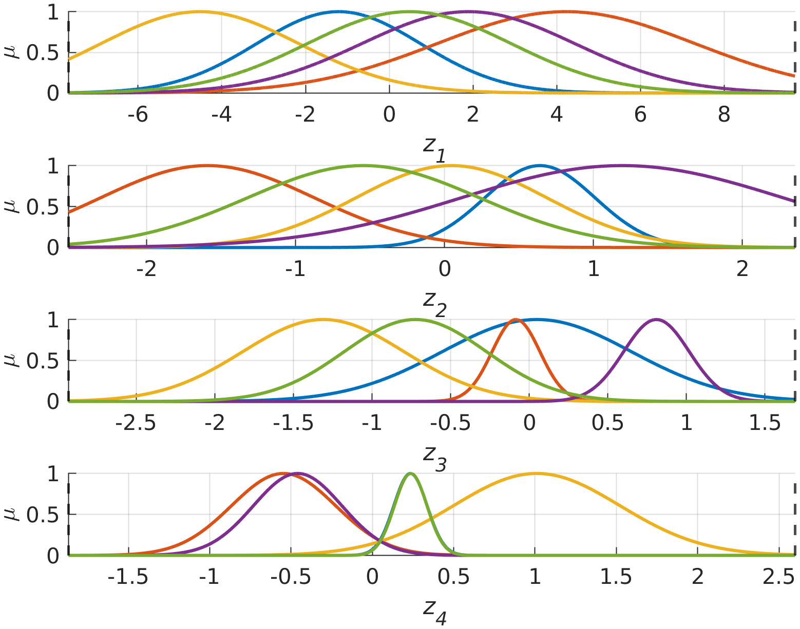
(a) FAM(4): $L_{2}$

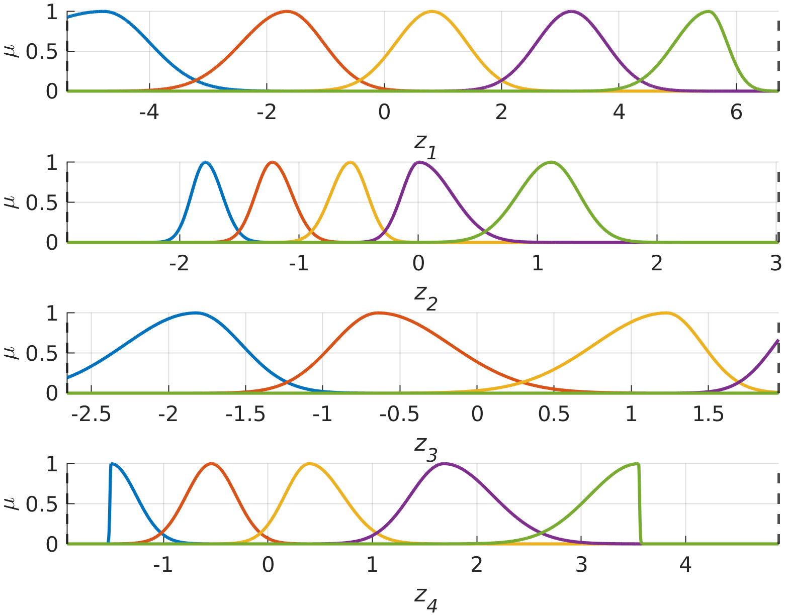
(b) FAME(4): $L_{2}$

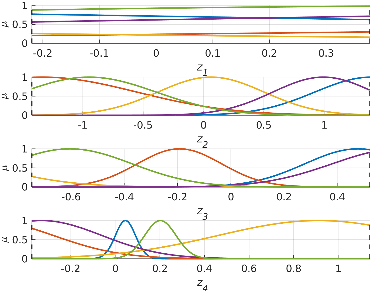
(c) FAM(4): $L_{F}$

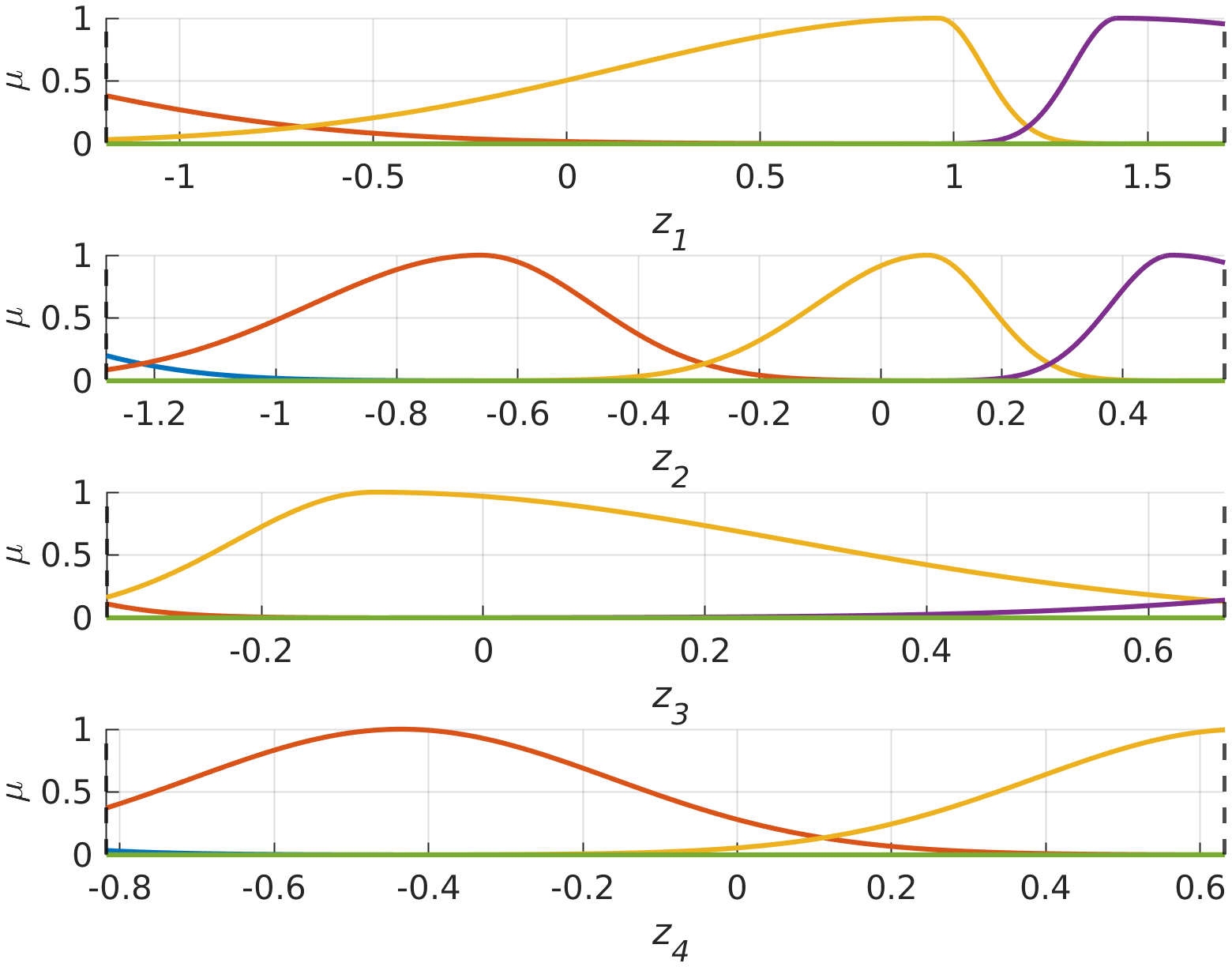
(d) FAME(4): $L_{F}$

Figure 2: Visualization of MFs in the effective universe of discourse, defined by the max and min values of learned $z_{i}$’s, and indicated by dashed lines.

We trained all FLSs with $P=5$ rules and used the same learning rate of $0.01$, a regularization parameter value $\lambda=0.05$, and mini-batch size (mbs) of $64$ for $100$ epochs. For the PM dataset, training was extended to $1000$ epochs with $mbs=512$. FLSs with a PL were trained using both $L_{2}$ and $L_{F}$ losses with $D=\{2,4,8\}$, while those without a PL were trained with only the $L_{2}$ loss. All experiments were conducted in MATLAB^® and repeated with 10 different initial seeds for statistical analysis.

TABLE II: Performance Analysis of FAM with $L_{2}$ over 10 Experiments

Dataset	Metric	V-MFLS	V-FAM	FAM(2)	FAM(4)	FAM(8)
ABA	#LP	125	160	58	116	232
	RMSE	67.24($\pm$2.08)	67.07($\pm$1.72)	66.01($\pm$1.86)	65.83($\pm$1.81)	66.07($\pm$1.75)
AIDS	#LP	350	460	88	176	352
	RMSE	70.16($\pm$1.36)	70.72($\pm$2.08)	67.61($\pm$1.86)	69.35($\pm$1.71)	73.08($\pm$3.56)
BH	#LP	200	260	68	136	272
	RMSE	42.01($\pm$2.71)	41.53($\pm$4.20)	41.44($\pm$6.74)	42.93($\pm$4.61)	42.27($\pm$5.51)
PM	#LP	290	380	80	160	320
	RMSE	65.00($\pm$3.93)	79.72($\pm$2.13)	71.00($\pm$2.62)	52.69($\pm$5.12)	39.50($\pm$4.81)
WW	#LP	170	220	64	128	256
	RMSE	80.61($\pm$1.55)	80.67($\pm$1.43)	83.06($\pm$1.84)	81.15($\pm$2.60)	81.70($\pm$4.00)
CS	#LP	125	160	58	116	232
	RMSE	36.01($\pm$2.48)	36.92($\pm$1.27)	43.89($\pm$1.28)	38.49($\pm$1.76)	34.49($\pm$1.64)

TABLE III: Performance Analysis of FAM with $L_{F}$ Over 10 Experiments

Dataset	Metric	V-MFLS	V-FAM	FAM(2)	FAM(4)	FAM(8)
ABA	#LP	125	160	58	116	232
	RMSE	67.24($\pm$2.08)	67.07($\pm$1.72)	65.67($\pm$1.70)	65.76($\pm$1.68)	65.73($\pm$1.64)
AIDS	#LP	350	460	88	176	352
	RMSE	70.16($\pm$1.36)	70.72($\pm$2.08)	67.65($\pm$2.24)	69.13($\pm$1.96)	70.77($\pm$2.84)
BH	#LP	200	260	68	136	272
	RMSE	42.01($\pm$2.71)	41.53($\pm$4.20)	43.64($\pm$5.40)	41.26($\pm$3.67)	40.25($\pm$6.60)
PM	#LP	290	380	80	160	320
	RMSE	65.00($\pm$3.93)	79.72($\pm$2.13)	73.07($\pm$1.99)	63.10($\pm$2.70)	49.28($\pm$2.70)
WW	#LP	170	220	64	128	256
	RMSE	80.61($\pm$1.55)	80.67($\pm$1.43)	82.72($\pm$1.84)	80.47($\pm$1.46)	79.96($\pm$1.04)
CS	#LP	125	160	58	116	232
	RMSE	36.01($\pm$2.48)	36.92($\pm$1.27)	42.79($\pm$1.94)	39.38($\pm$1.45)	36.99($\pm$2.83)

TABLE IV: Performance Analysis of FAME with $L_{2}$ Over 10 Experiments

Dataset	Metric	V-MFLSE	V-FAME	FAME(2)	FAME(4)	FAME(8)
ABA	#LP	101	136	52	104	208
	RMSE	67.25($\pm$2.24)	68.40($\pm$1.98)	66.30($\pm$2.05)	65.31($\pm$2.05)	65.44($\pm$1.37)
AIDS	#LP	281	391	82	164	328
	RMSE	70.52($\pm$2.20)	71.21($\pm$2.27)	71.99($\pm$3.71)	71.15($\pm$2.11)	74.57($\pm$2.60)
BH	#LP	161	221	62	124	248
	RMSE	43.37($\pm$5.32)	43.08($\pm$4.17)	44.90($\pm$5.96)	46.33($\pm$3.32)	45.60($\pm$6.42)
PM	#LP	233	323	74	148	296
	RMSE	79.13($\pm$3.46)	81.01($\pm$1.61)	77.34($\pm$2.36)	61.60($\pm$2.73)	44.79($\pm$4.93)
WW	#LP	137	187	58	116	232
	RMSE	82.32($\pm$1.33)	81.13($\pm$1.60)	83.24($\pm$1.96)	80.69($\pm$1.44)	81.22($\pm$2.15)
CS	#LP	101	136	52	104	208
	RMSE	43.75($\pm$4.31)	38.88($\pm$1.61)	58.73($\pm$14.04)	41.79($\pm$2.88)	38.98($\pm$3.43)

TABLE V: Performance Analysis of FAME with $L_{F}$ Over 10 Experiments

Dataset	Metric	V-MFLSE	V-FAME	FAME(2)	FAME(4)	FAME(8)
ABA	#LP	101	136	52	104	208
	RMSE	67.25($\pm$2.24)	68.40($\pm$1.98)	66.55($\pm$2.16)	65.44($\pm$1.85)	65.74($\pm$2.12)
AIDS	#LP	281	391	82	164	328
	RMSE	70.52($\pm$2.20)	71.21($\pm$2.27)	70.78($\pm$4.34)	68.11($\pm$2.05)	69.59($\pm$2.28)
BH	#LP	161	221	62	124	248
	RMSE	43.37($\pm$5.32)	43.08($\pm$4.17)	43.96($\pm$6.44)	42.76($\pm$6.17)	39.66($\pm$4.85)
PM	#LP	233	323	74	148	296
	RMSE	79.13($\pm$3.46)	81.01($\pm$1.61)	77.78($\pm$2.29)	64.04($\pm$5.91)	57.28($\pm$4.17)
WW	#LP	137	187	58	116	232
	RMSE	82.32($\pm$1.33)	81.13($\pm$1.60)	82.97($\pm$1.58)	80.91($\pm$1.23)	80.76($\pm$1.53)
CS	#LP	101	136	52	104	208
	RMSE	43.75($\pm$4.31)	38.88($\pm$1.61)	51.30($\pm$9.43)	41.19($\pm$1.98)	36.67($\pm$2.07)

• (1) RMSE values are scaled by 100.

• (2) Measures that are highlighted indicate the best performance.

IV-B Impact of Feature Space on FAM and FAME Performance

Table V-V summarizes RMSE values of FAM and FAME over 10 experiments for both the deployment of $L_{2}$ and $L_{f}$ alongside their #LP. Here, FAM and FAME with $D=\{2,4,8\}$ are referred to as $\text{FAM}(D)$ or $\text{FAME}(D)$, respectively. To define a baseline performance, we also included the results of V-MFLS. We observe that:

• V-FAM and V-FAME, which are additive models, perform similarly to V-MFLS and V-MFLSE. FAM($D$) and FAME($D$), additive models equipped with a PL, outperform them. Yet, the setting of $D$ depends on the dataset, emphasizing its importance as a key hyperparameter.

• FAM typically achieves better performance than FAME. This outcome is anticipated because FAME’s reduced number of LPs limits its learning capacity, often resulting in lower performance compared to FAM.

• FAM and FAME exhibit comparable performance regardless of whether $L_{2}$ or $L_{F}$ is used.

Now, let us examine how the antecedent space is shaped after training. Fig. 2 shows the learned MFs from an ABA experiment, where FAM achieved a slightly better RMSE value. Here, we plot the effective universe of discourse of the antecedent MFs, defined as the range of $z_{i}$ obtained after training (i.e., max and min values). Observe that:

• In Fig. 2(a), the MFs of FAM overlap, making it difficult to assign distinct linguistic labels. For example, around $z_{1}=0$, multiple MFs could share the same label. In contrast, FAME shows improved interpretability by limiting the active MFs to at most two for any $z_{i}$ making it easier to label the MFs, as shown in Fig. 2(b). We also observe input spaces defined by one MF in FAME where a single rule is learned to represent this input range. This simplifies the model and improves interpretability by reducing the complexity of the rules learned.

• The impact of the loss is evident in Fig. 2, where $L_{F}$ results in a narrower effective universe of discourse compared to $L_{2}$. Fig. 2(c) highlights the challenge of interpreting the FAM as all MFs overlap. Unlike for FAME, we observe from Fig. 2(d) that the number of interpretable MFs within effective input space is reduced, and thus fewer rules are needed for explanation.

In conclusion, the choice between FAM and FAME depends on the balance between explainability and performance. Yet, FAME with $L_{F}$ improves interpretability by reducing the number of rules and offering clearer linguistic labels for antecedents when compared to FAM at a slight cost to accuracy.

IV-C Assessing the Performance of FAM and FAME vs MFLS

In Table VI and Table VII, we show the RMSE values for all trained FLSs over 10 experiments using $L_{2}$ and $L_{F}$ loss functions, respectively. Here, we only reported the results of FLSs with a PL (FAM, FAME, CDR, and DR) with their best hyperparameter setting of $D$ selected from $D=\{2,4,8\}$. We also provided the rankings over the handled 6 datasets for an easy comparison for each model. We can observe that:

• FAM/FAME generally exhibits competitive performances. Notably, FAM shows the best overall performance according to average rankings.

• FAME is a robust performer as it is in the top 3 in both average ranks while also resulting in interpretability and a manageable active set of rules.

• FAM/FAME has a better performance compared to its vanilla counterparts. This shows PL has a positive effect.

In summary, we conclude that FAM and FAME do not result in accuracy decrements compared to their MFLS counterparts, despite being based on SFLSs, which also process input interactions. FAME, in particular, is generally a robust performer across all datasets, with the added benefit of interpretability.

TABLE VI: Performance Analysis of Best of All with $L_{2}$ Over 10 Experiments

Dataset	Metric	FAM	V-FAM	FAME	V-FAME	V-MFLS	V-MFLSE	CDR-MFLS	CDR-MFLSE	DR-MFLS	DR-MFLSE
ABA	#LP	116	160	104	136	125	101	53	173	83	173
	RMSE	65.83($\pm$1.81)	67.07($\pm$1.72)	65.31($\pm$2.05)	68.40($\pm$1.98)	67.24($\pm$2.08)	67.25($\pm$2.24)	66.39($\pm$1.82)	66.22($\pm$1.54)	66.73($\pm$1.91)	66.17($\pm$1.59)
AIDS	#LP	88	460	164	391	350	281	83	77	188	182
	RMSE	67.61($\pm$1.86)	70.72($\pm$2.08)	71.15($\pm$2.11)	71.21($\pm$2.27)	70.16($\pm$1.36)	70.52($\pm$2.20)	65.97($\pm$2.81)	69.25($\pm$3.08)	71.52($\pm$2.29)	71.40($\pm$2.65)
BH	#LP	68	260	62	221	200	161	63	57	118	238
	RMSE	41.44($\pm$6.74)	41.53($\pm$4.20)	44.90($\pm$5.96)	43.08($\pm$4.17)	42.01($\pm$2.71)	43.37($\pm$5.32)	43.54($\pm$5.25)	46.81($\pm$6.75)	42.37($\pm$6.14)	44.09($\pm$6.03)
PM	#LP	320	380	296	323	290	233	285	261	340	316
	RMSE	39.50($\pm$4.81)	79.72($\pm$2.13)	44.79($\pm$4.93)	81.01($\pm$1.61)	65.00($\pm$3.93)	79.13($\pm$3.46)	46.45($\pm$3.91)	56.33($\pm$5.99)	47.42($\pm$6.25)	53.60($\pm$2.83)
WW	#LP	128	220	116	187	170	137	113	197	104	212
	RMSE	81.15($\pm$2.60)	80.67($\pm$1.43)	80.69($\pm$1.44)	81.13($\pm$1.60)	80.61($\pm$1.55)	82.32($\pm$1.33)	81.70($\pm$2.43)	81.17($\pm$1.94)	81.05($\pm$1.66)	80.90($\pm$2.15)
CS	#LP	232	160	208	136	125	101	197	173	197	173
	RMSE	34.49($\pm$1.64)	36.92($\pm$1.27)	38.98($\pm$3.43)	38.88($\pm$1.61)	36.01($\pm$2.48)	43.75($\pm$4.31)	41.35($\pm$3.90)	44.18($\pm$3.75)	40.78($\pm$3.80)	40.64($\pm$2.63)
Average Rank		2.34	4.84	4.50	7.17	4.17	7.84	5.50	6.84	6.00	5.84

TABLE VII: Performance Analysis of Best of All with $L_{F}$ Over 10 Experiments

Dataset	Metric	FAM	V-FAM	FAME	V-FAME	V-MFLS	V-MFLSE	CDR-MFLS	CDR-MFLSE	DR-MFLS	DR-MFLSE
ABA	#LP	58	160	104	136	125	101	101	89	121	173
	RMSE	65.67($\pm$1.70)	67.07($\pm$1.72)	65.44($\pm$1.85)	68.40($\pm$1.98)	67.24($\pm$2.08)	67.25($\pm$2.24)	65.60($\pm$1.76)	65.49($\pm$1.87)	66.12($\pm$1.72)	65.68($\pm$1.82)
AIDS	#LP	88	460	164	391	350	281	83	77	188	182
	RMSE	67.65($\pm$2.24)	70.72($\pm$2.08)	68.11($\pm$2.05)	71.21($\pm$2.27)	70.16($\pm$1.36)	70.52($\pm$2.20)	66.31($\pm$1.52)	67.83($\pm$2.11)	69.28($\pm$2.36)	70.06($\pm$2.34)
BH	#LP	272	260	248	221	200	161	121	213	262	238
	RMSE	40.25($\pm$6.60)	41.53($\pm$4.20)	39.66($\pm$4.85)	43.08($\pm$4.17)	42.01($\pm$2.71)	43.37($\pm$5.32)	41.25($\pm$6.23)	42.62($\pm$6.60)	41.11($\pm$6.08)	38.42($\pm$4.90)
PM	#LP	320	380	296	323	290	233	285	261	340	316
	RMSE	49.28($\pm$2.70)	79.72($\pm$2.13)	57.28($\pm$4.17)	81.01($\pm$1.61)	65.00($\pm$3.93)	79.13($\pm$3.46)	44.94($\pm$5.39)	55.26($\pm$3.09)	46.17($\pm$6.70)	56.51($\pm$2.23)
WW	#LP	256	220	232	187	170	137	221	197	148	212
	RMSE	79.96($\pm$1.04)	80.67($\pm$1.43)	80.76($\pm$1.53)	81.13($\pm$1.60)	80.61($\pm$1.55)	82.32($\pm$1.33)	80.22($\pm$1.72)	79.98($\pm$1.74)	80.07($\pm$1.08)	80.05($\pm$1.25)
CS	#LP	232	160	208	136	125	101	197	173	197	173
	RMSE	36.99($\pm$2.83)	36.92($\pm$1.27)	36.67($\pm$2.07)	38.88($\pm$1.61)	36.01($\pm$2.48)	43.75($\pm$4.31)	38.97($\pm$2.37)	38.17($\pm$1.59)	37.67($\pm$1.54)	38.25($\pm$2.61)
Average Rank		2.84	6.84	3.84	9.34	6.00	9.17	4.00	4.17	4.34	4.50

• RMSE values are scaled by 100.

• The bold values are the best results in each row.

V Conclusion and Future Work

In this study, we introduce FAM and FAME, which leverage the strengths of additive models and SFLSs, making them ideal solutions for XAI. The proposed FAME, incorporating a novel parameterization of MFs, efficiently captures input-output relationships with fewer active rules. The presented comparative results show that both FAM and FAME are comparable to traditional MFLSs, with FAM often providing slightly higher accuracy and FAME excelling in interpretability, making it ideal for applications where explainability is crucial. Ultimately, the selection between FAM and FAME depends on the required balance between accuracy and explainability. Our findings demonstrate that these models not only perform well across various datasets but also significantly improve interpretability.

Future work will be on investigating low-dimensional space $\boldsymbol{Z}\in\mathbb{R}^{D\times 1}$ and consequent space of FAME to provide an end-to-end interpretable fuzzy family for XAI.

References

- [1] D. Minh, H. X. Wang, Y. F. Li, and T. N. Nguyen, “Explainable artificial intelligence: a comprehensive review,” Artificial Intelligence Review, pp. 1–66, 2022.
- [2] R. Agarwal, L. Melnick, N. Frosst, X. Zhang, B. Lengerich, R. Caruana, and G. E. Hinton, “Neural additive models: Interpretable machine learning with neural nets,” in Adv. Neural Inf. Process Syst., vol. 34, 2021, pp. 4699–4711.
- [3] Z. Yang, A. Zhang, and A. Sudjianto, “Enhancing explainability of neural networks through architecture constraints,” IEEE Trans. Neural Netw. Learn. Syst., vol. 32, no. 6, pp. 2610–2621, 2021.
- [4] ——, “Gami-net: An explainable neural network based on generalized additive models with structured interactions,” Pattern Recognition, vol. 120, p. 108192, 2021.
- [5] J. Vaughan, A. Sudjianto, E. Brahimi, J. Chen, and V. N. Nair, “Explainable neural networks based on additive index models,” arXiv preprint arXiv:1806.01933, 2018.
- [6] C. He, M. Ma, and P. Wang, “Extract interpretability-accuracy balanced rules from artificial neural networks: A review,” Neurocomputing, vol. 387, pp. 346–358, 2020.
- [7] O. Cordón, “A historical review of evolutionary learning methods for mamdani-type fuzzy rule-based systems: Designing interpretable genetic fuzzy systems,” Int. J. Approx. Reason., vol. 52, no. 6, pp. 894–913, 2011.
- [8] H. Hagras, “Toward human-understandable, explainable ai,” Computer, vol. 51, no. 9, pp. 28–36, 2018.
- [9] A. Fernandez, F. Herrera, O. Cordon, M. Jose del Jesus, and F. Marcelloni, “Evolutionary fuzzy systems for explainable artificial intelligence: Why, when, what for, and where to?” IEEE Comput. Intell. Mag., vol. 14, no. 1, pp. 69–81, 2019.
- [10] J. M. Mendel and P. P. Bonissone, “Critical thinking about explainable ai (xai) for rule-based fuzzy systems,” IEEE Trans. Fuzzy Syst., vol. 29, no. 12, pp. 3579–3593, 2021.
- [11] Z. Shi, S. Huang, L. Wu, Q. Zhang, X. Zhang, Y. Cao, Y. Chen, and Y. Lv, “Tsk fuzzy system optimization for high-dimensional regression problems,” IEEE Trans. Emerg. Top. Comput. Intell., 2024.
- [12] Y. Cui, D. Wu, and Y. Xu, “Curse of dimensionality for tsk fuzzy neural networks: Explanation and solutions,” in Proc. Int. Jt. Conf. Neural Netw., 2021.
- [13] C. L. P. Chen, C.-Y. Zhang, L. Chen, and M. Gan, “Fuzzy restricted boltzmann machine for the enhancement of deep learning,” IEEE Trans. Fuzzy Syst., vol. 23, no. 6, pp. 2163–2173, 2015.
- [14] S. Park, S. J. Lee, E. Weiss, and Y. Motai, “Intra- and inter-fractional variation prediction of lung tumors using fuzzy deep learning,” IEEE J. Trans. Eng. Health. Med., vol. 4, pp. 1–12, 2016.
- [15] S. Rajurkar and N. K. Verma, “Developing deep fuzzy network with takagi sugeno fuzzy inference system,” in IEEE International Conference on Fuzzy Systems, 2017, pp. 1–6.
- [16] R. Chimatapu, H. Hagras, A. Starkey, and G. Owusu, “Interval type-2 fuzzy logic based stacked autoencoder deep neural network for generating explainable ai models in workforce optimization,” in IEEE International Conference on Fuzzy Systems, 2018.
- [17] ——, “Explainable ai and fuzzy logic systems,” in Theory and Practice of Natural Computing, 2018.
- [18] T. Kumbasar, “Robust stability analysis and systematic design of single-input interval type-2 fuzzy logic controllers,” IEEE Trans. Fuzzy Syst., vol. 24, no. 3, pp. 675–694, 2016.
- [19] Y. Güven, A. Köklü, and T. Kumbasar, “Exploring Zadeh’s General Type-2 Fuzzy Logic Systems for Uncertainty Quantification,” IEEE Trans. Fuzzy Syst., 2024.
- [20] A. Köklü, Y. Güven, and T. Kumbasar, “Odyssey of interval type-2 fuzzy logic systems: Learning strategies for uncertainty quantification,” IEEE Trans. Fuzzy Syst., pp. 1–10, 2024.
- [21] A. Köklü, Y. Güven, and T. Kumbasar, “Efficient learning of fuzzy logic systems for large-scale data using deep learning,” in International Conference on Intelligent and Fuzzy Systems, 2024.
- [22] Y. Cui, Y. Xu, R. Peng, and D. Wu, “Layer normalization for tsk fuzzy system optimization in regression problems,” IEEE Trans. Fuzzy Syst., vol. 31, no. 1, pp. 254–264, 2023.