Journal reference: Journal of Nonlinear Science DOI: 10.1007/s00332-025-10152-9
The FitzHugh-Nagumo System on Undulated Cylinders: Spontaneous Symmetrization and Effective System
Abstract.
We consider the FitzHugh-Nagumo system on undulated cylindrical surfaces modeling nerve axons. We show that for sufficiently small radii and for initial conditions close to radially symmetrical ones, (i) the solutions converge to their radial averages, and (ii) the latter averages can be approximated by solutions of a dimensional (‘radial’) system (the effective system) involving the surface radius function in its coefficients. This perhaps explains why solutions of the original dimensional FitzHugh-Nagumo system agree so well with experimental data on electrical impulse propagation.
Key words and phrases:
electric impulse, neurons, axons, Hodgkin-Huxley model, FitzHugh–Nagumo equations, pulse, traveling wave, propagation, solitary wave.1991 Mathematics Subject Classification:
35C07, 37N25, 35Q92, 35B07, 35K57, 46N60, 92-08, 92-10, 92C20, 35K911. Introduction
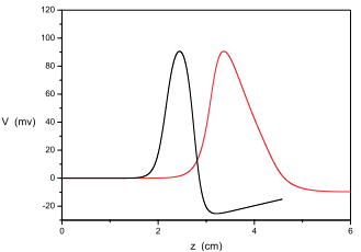
The FitzHugh-Nagumo (FHN) system describes propagation of electrical impulses (pulses) along nerve filaments (axons). It is a simplification of the Nobel prize winning Hodgkin-Huxley (HH) system with slow unknown variables of ion concentrations, whose movement through the axon surface creates the potential gradient, clumped into a single slow variable. Despite this simplification, the FHN system provides a remarkably accurate qualitative and in many cases quantitative description of the rather complicated phenomenon of signal propagation along nerve cells. For comparison between the HH and FHN pulse profiles (as functions of a real variable representing a moving frame coordinate ), see [33] and Fig. 1 below.
Though axons are thin tubes of variable radii and of complicated geometry, with electrical impulses propagating on their surfaces, starting with the Hodgkin and Huxley work [17], they are modeled by straight lines with no internal structure. To address this discrepancy, it was proposed by Talidou et al. [37] to model axons by thin cylindrical surfaces and to extend the FitzHugh-Nagumo system (FHN) to such a surface, , as
| (1.1) |
where is the Laplace-Beltrami operator on a surface . The function is the cubic polynomial
| (1.2) |
for The constants and are positive and sufficiently small, . Apart from replacing by the FHN system is not changed. Thus, for and consequently Eq. (1.1) is reduced to the standard FitzHugh-Nagumo system (1), in our notation, on (which does not involve ).
Specifically, [37] considers (1.1) on cylindrical surfaces, , called there the warped cylinders, whose radii vary slowly along their length and with the change of the azimuthal angle, defined as a graph over the standard cylinder, ,
| (1.3) |
where is the polar angle and is a slowly varying function of The only difference with the standard FHN system (1) is in replacing the second derivative by the surface Laplacian.
Besides providing the next natural step in modeling pulse dynamics in axons, Eq. (1.1) is an interesting mathematical model for propagation of traveling waves on surfaces.
In this paper, we study general properties of solutions for very thin cylindrical surfaces and emergence of 1D effective systems. To explain the issues involved, we consider Eq. (1.1) first on where is the surface of a straight cylinder, , of a constant radius centered about the -axis in . We parametrize by the cylindrical coordinates as
| (1.4) |
with the Riemannian area element and the Laplacian given by and
| (1.5) |
Clearly, each solution of Eq. (1) defines a radial, i.e. axi-symmetric, or -independent, solution of Eq. (1.1) for for any and vice versa.
Like Eq. (1), Eq. (1.1) for denoted (1), is invariant under translations, i.e., if is a solution, then so are its translates
Hence Eq. (1) might have traveling wave solutions. It is known that for , Eq. (1) has two traveling wave solutions, fast and slow, the first of which is stable while the second unstable (see [13, 11, 20]).
More precisely (see [37]), for and , are positive and sufficiently small, Eq. (1) has at least two different pulse solutions, the fast pulse (shown in Fig. 1), which travels with speed , and a slow pulse that travels with speed (Hastings [15, 16], Carpenter [4], Langer [27], Jones, Kopell and Langer [23], Krupa, Sandstede and Szmolyan [26], Arioli and Koch [2]). The uniqueness of the fast pulse was proven by Langer [27]. Furthermore, the fast pulse is stable (Jones [22] and Yanagida [39]), while the slow pulse is unstable (Flores [13], Evans [11], Ikeda, Mimura and Tsujikawa [20]). In addition, there are stable fast pulses with oscillatory tails (Carter and Sandstede [6], Carter, de Rijk and Sandstede [5]).
By above, each pulse on defines a smooth axisymmetric traveling wave solution of Eq. (1), propagating along the cylindrical axis. Its speed is determined by the parameters , , and . After [37], we continue to call them the pulses. We are interested in the fast pulse, for which we keep the notation .
Results of [37].
As was mentioned above, an analysis of the FHN system (1) on cylindrical surfaces was initiated in [37]. It is shown in [37] that, for with mild solutions which are initially close to approach nearby translates of as , or put differently,
-
(i)
On a cylinder of small constant radius, the (fast) pulses are asymptotically orbitally stable under general perturbations of the initial conditions that depend on both spatial variables.
One does not expect that there are pulse-like traveling waves on generic cylindrical surfaces, , even if is close to a constant . However, it is shown in [37] that:
-
(ii)
Eq. (1), for the warped cylinder has stable, nearly radial pulses surrounded by small fluctuations propagating along the cylindrical axis (as is the case with real axons).
Put differently, on a warped cylinder, solutions that are initially close to a pulse stay near a propagating pulse for all time. (Note that the restriction is not optimal. In particular, we conjecture that the results of [37] hold for However, the optimal interval of for which the results of [37] hold is not known. We thank an anonymous referee for posing this question.)
In this paper, we consider the undulated cylinders, i.e. graphs, (1.3), over standard cylinders with the defining radius function, radially symmetric, i.e. depending only on , . We prove:
-
•
A spontaneous symmetrization of solutions, initially close to radially symmetric ones;
- •
To formulate our results precisely, we let be the Hilbert space of square integrable functions on (see (1.18) below for more a detailed description) and define the vector Sobolev space, in a standard way as
| (1.6) |
where is the Laplace-Beltrami operator on (see (1.20) below) and , with norm
| (1.7) |
and its dual Furthermore, we say (1) has a strong, local solution in if
for some and satisfies Eq. (1). We say that the solution u is global if we can take
Consider (1) with of class , bounded and radially symmetric (i.e. independent of ) with We consider strong solutions of this equation on an interval satisfying
| (1.8) |
where , and denote the class of such solutions by
A local existence of (1) on with independent of the parameters and is standard and is discussed in Appendix A. It is proven in exactly the same way as a higher regularity local existence is proven in [37], Proposition 2.1. One can readily show that the local solutions satisfy (1.8) with constants independent of and so that the sets are definitely non-empty.
Below, we prove a priori bounds on solutions of (1) independent of the existence results.
Our first result is given in:
Theorem 1.1.
There exist and s.t., for any and any and any strong solution to (1) in with an initial condition obeying , satisfies the estimate
| (1.9) |
where is a positive constant independent of and .
Remarks 1.
(i) We expect that for initial conditions in Theorem 1.1, the solutions exist and belong to and Let
(cf. (A.1) in Appendix A) with the norm and define the manifold of pulses
where, recall, Let also It is shown in [37, Theorem 1.2] that there are such that if for some then for any initial condition s.t. there exists the unique global solution of (1) satisfying for some constant independent of The latter bound implies that and therefore with and
(ii) Unlike in the results of [37], the surfaces in Theorem 1.1 are not assumed to be closed to a straight cylinder.
(iii) The results above depend strongly on the sectional curvatures of the sections of by planes orthogonal to the -axis. In particular, in Theorem 1.1 is the lower bound on It is crucial here that the new -degree of freedom is compact.
Surprisingly, the result above is independent of the principal curvature along -axis and depends only on the line element along
We conjecture that our result extend to warped surfaces, i.e. to dependent not only on but also on
We also introduce the radial and Sobolev spaces in 1 dimension
| (1.10) | ||||
| (1.11) |
where is the radial part of the Laplace-Beltrami operator see (1.21) and (1.20) below, with the norms defined as in (1.7) (actually, they could be defined by (1.7)) and denoted by the same symbols and similarly for the scalar products. Moreover, we also use the dual space to
The next result compares the averages of solutions to (1) to solutions of the following system of equations
| (1.12) |
We consider strong solutions of Eqs (1) and (1.12) in the spaces
We have:
Theorem 1.2.
Under the conditions of Theorem 1.1, the average of the strong solution of (1) in and the strong solution in to (1.12), with initial conditions and , respectively, satisfy the estimate
| (1.13) |
for some constants independent of and and
A proof of Theorem 1.2 is given in Section 3. Eq. (1.12) is a system in 1 spatial dimension depending on the radius profile It is considerably simpler for mathematical analysis and numerical simulations, and will be explored in a future study. It offers an effective system for the pulse propagation.
Remarks 2.
(i) To keep exposition simple, we restricted ourselves to the energy space It would be interesting to extend the results above to higher regularity. It is natural to use Sobolev spaces with different smoothness in different components, since (1) is of the second order in and the zero order in
(ii) The global existence in the space defined in Remark 1(i) and Appendix A, for certain class of initial data is proven in [37]. One might be able to extend the proof of [37] to under conditions similar to those of [37].
(iii) There are a few results in higher dimensions. In , Mikhailov and Krinskii [30], and Keener [25] studied spiral solutions of Eq. (1). In -dimensions, for , Tsujikawa, Nagai, Mimura, Kobayashi and Ikeda [38] proved that there exist stable fast pulse solutions propagating in a one-dimensional direction. Numerical computation of solitary waves in cylindrical domains was done in [28] (see [35] for a review and further references).
(iv) Existence and stability for fast pulses have been studied for variants of Eq. (1), where the second equation also has a diffusion term (Cornwell and Jones [9], Chen and Choi [7], Chen and Hu [8]). It would be interesting to extend the results above to undulated surfaces variants of these equations.
(v) Another system that admits stable fast pulses is the discrete analogue of Eq. (1) (Hupkes and Sandstede [19], Schouten-Straatman and Hupkes [36], Hupkes, Morelli, Schouten-Straatman and Van Vleck [18]).
(vi) Another natural extension of Eq. (1.1) would be to have an -dependent nonlinearity modeling varying mylination.
Outline of the approach.
Our main tool is the method of differential inequalities for quadratic functionals (cf. [1, 14, 24] and references therein). Namely, combining the functionals
| (1.14) |
with , where and
| (1.15) |
where into a simple functional we obtain the differential inequality, for where is a solution of (1) in
Integrating this inequality (see abstract Lemma 2.2) and using that we arrive at Eq. (1.9).
Theorem 1.2 is proven similarly, except that the coefficient in front of an equivalent of is positive which gives a time growing exponential. The later result could possibly be improved but this would require additional powerful machinery, similar to that used in [37], such as detailed spectral analysis of the linearized system and comparison estimates for solutions of (1) and (1).
The paper is organized as follows. In Section 2, we give a proof of Theorem 1.1 with technical estimates carried in Section 2.2. In Section 3, we prove Theorem 1.2 and in Appendix A, we sketch a proof of the local existence for system (1).
We conclude the introduction with a discussion of the spaces used in this work.
Remarks on spaces and operators.
In the cylindrical coordinates, undulated cylindrical surface cf. (1.3), is written as
| (1.16) |
and the area element on is given by , where is the determinant of the metric tensor, defined in (1.21),
| (1.17) |
In the cylindrical coordinates, the space is identified with
| (1.18) |
where, recall, and . We define the inner product on as
| (1.19) |
The corresponding norm will be denoted by . The scaling in (1.19) was introduced in [37] in order to make the linearized operator (1.15) symmetric.
Turning to the Laplace-Beltrami operator on with independent of which we use to define the Sobolev spaces, in the cylindrical coordinates, it is given by
| (1.20) |
where, recall, and is given in (1.17). The operator is self-adjoint and non-positive on the space of scalar -functions on (cf. (1.18)).
The radial part of the Laplace-Beltrami operator is given by
| (1.21) |
Notation.
To summarize, we denote the and Sobolev spaces as and
for scalar functions, and as and for the vector functions.
In what follows, the norms in and , are denoted by and respectively. The function is fixed and we omit it in the notation, except for the notation for the cylindrical surface.
Furthermore, the parameters and and the function entering (1), (1.2) are fixed positive numbers. is essential in the stability theory and we trace the dependence on it while ignoring and etc are arbitrary constants independent of and These constants may depend on and and the Sobolev constants and may vary from one inequality to another. The maximum of various Sobolev constants in 1D and 2D is denoted by The constants used in Sections 2 and 3 are not related to each other.
Finally, for two positive functions and the notation say that for some positive constants, which might depend on and but are independent on and
We use the following typographical convention. Constants are denoted by lower greek and capital roman letters (e.g. etc), operators, by roman capitals (e.g. ), functions by either lower or capital roman letters (e.g. or to eliminate the confusion in the latter case, we display the arguments, i.e. and ), and maps, by capital math calligraphic letters (e.g. and ). The only exception is the function Vector functions are denoted by boldface letters, e.g.
2. Angular contraction: Proof of Theorem 1.1
2.1. Proof of Theorem 1.1 modulo estimates (2.21) and (2.22)
In this subsection we prove Theorem 1.1 modulo two key technical estimates demonstrated in the next subsection. We split the proof of Theorem 1.1 into several steps.
To begin with, we observe that on the cylindrical surface , the FHNcyl system, (1), takes the form
| (2.1) |
where the Laplace-Beltrami operator on (see (1.20) for an explicit expression).
Canonical form of equation (2.1).
Denote the right hand side of Eq. (2.1) by . Then the initial-value problem for (2.1) becomes
| (2.2) |
We consider this problem on the space . We rewrite the initial-value problem Eq. (2.2) by expanding in u and using to obtain
| (2.3) |
where and is defined by this equation, namely, . Now, Eq. (2.2) becomes
| (2.4) |
where is the principal part of given by its Gâteaux derivative at
| (2.5) |
with the Laplace-Beltrami operator given in (1.20), and is the nonlinear part (nonlinearity) given by
| (2.6) |
Operator .
Recall the space and define the space as
| (2.7) |
By the standard elliptic theory, the Gâteaux derivative maps into for (see [37]).
Lyapunov-Schmidt decomposition.
Let be the projection on the average of the function in (zero harmonic):
| (2.8) |
and similarly for vector-functions, and let . Note that the operators commute with (on scalar functions) and with (on vector-functions). Furthermore, let
| (2.9) |
| (2.10) |
Note that, since is radially symmetric, the operator commutes with the rotations and therefore with and .
Lyapunov functions
To estimate various norms of we use differential inequalities for the following Lyapunov functions
| (2.12) |
with . Note that and, as shown below, that
Recall that is defined in (1.20), and let be the corresponding gradient. Using the formula (1.20) and then integrating by parts, we find
| (2.13) |
Using the definition of in (1.15) and the definition of the inner product in (1.19) and using the relation (2.13), we obtain
| (2.15) | |||||
| (2.16) |
where recall the notation says that and satisfy for some positive constants depending on the fixed parameters and of Eq. (1).
The point here is that on the operator is coercive: for any
| (2.17) |
with , provided Indeed, using (2.5) and the inner product (1.19), we compute
| (2.18) |
where is defined according to (2.10). Writing and using that and the inequality (2.19) given below, we find (2.17).
Lemma 2.1.
Let Then we have the estimate
| (2.19) |
Proof.
In the next subsection, assuming , we prove the following estimates (see Propositions 2.5 and 2.6): for any and
| (2.21) |
and
| (2.22) |
for some positive constants and independent of the parameters and and of the function and satisfying
| (2.23) |
Note that (2.21) implies a bound on For this, we use the following general result:
Lemma 2.2.
Let be a positive, differentiable function satisfying differential inequality
| (2.24) |
with an initial condition Then satisfies the estimate
| (2.25) |
Proof.
Let Then using (2.24), we obtain
| (2.26) |
Integrating this inequality, and taking the supremum of the result over the interval and using the notation
| (2.27) |
we obtain the inequality
| (2.28) |
For the polynomial has three roots (see Fig. 2)
In the proofs below, are numerical constants, independent, in particular, of the parameters and the function Subsequent constants depend on the preceding ones at most polynomially.
Proposition 2.3.
Assume Then we have
| (2.29) |
where with, recall,
Proof.
Corollary 2.4.
Recalling the definitions and , we arrive at the inequality
| (2.31) |
To prove a stronger bound, under the additional assumption we define the new, combined Lyapunov function
| (2.32) |
Differentiating and using (2.21) and (2.22), and absorbing the term into , we find
| (2.33) |
where, with as in (2.32),
Now, assuming for simplicity (recall that )
| (2.34) |
and using (2.32), (2.15) and the definitions of and we obtain
| (2.35a) | |||||
| (2.35b) | |||||
Dropping the last term in (2.33) and using (2.35b), we conclude that
| (2.36) |
where and are positive constants which appeared in (2.33) and which are independent of the parameters and
2.2. A priori estimates: Proof of (2.21) and (2.22)
In this subsection we prove estimates (2.21) and (2.22) used in subsection 2.1. With the function given in (2.12), we have:
Proposition 2.5.
Proof.
For the second term on the r.h.s. of (2.38), using definition (2.6), we transform
| (2.39) |
where is the first component of and is given in (2.6). Next, using that and , we expand
| (2.40) | ||||
| (2.41) |
Combining equations (2.39) and (2.40), together with (2.41) and the expressions
| (2.42) |
(see (2.6)), we arrive at
| (2.43) | |||||
Using (2.43), and using that (recall that ) for the first line in the r.h.s. of (2.43) and dropping the negative term from the second line, we find
Next, using Hölder estimate and the one-dimensional Sobolev embedding inequality and recalling that we find
| (2.44) |
Using (2.38), (2.17) and (2.44), we obtain
| (2.45) |
Next, we use the Gagliardo-Nirenberg-Sobolev inequality in the dimension :
| (2.46) |
with and and therefore . Applying this inequality to the last term in (2.45) and using
| (2.47a) | |||||
| (2.47b) | |||||
where , yields the estimate
| (2.48) |
Using that, by our conditions, and recalling that so that
| (2.49) |
with and recalling the notation we see that Eq. (2.48) yields (2.37). ∎
For the Lyapunov function given in (2.12), we prove the following:
Proposition 2.6.
Proof of Proposition 2.6.
Omitting the argument and using Eq. (2.11), that all the functions involved are real, and using the notation we compute
| (2.51) | |||||
where
| (2.52) | |||||
where is the adjoint of in the metric (see (1.19)). To estimate the nonlinear term we use the Cauchy-Schwarz inequality in (2.52) to find
| (2.53) |
Now, using (2.5), we compute
| (2.54) |
| (2.55) |
we obtain furthermore
| (2.56) | |||||
Using the estimate (2.56) in (2.51), we find
| (2.57) |
Now, we estimate the terms in the r.h.s. of (2.57). Using (2.5), the expression for the norm corresponding to the inner product (1.19), i.e. (1.7) for and the Cauchy-Schwarz inequality, we calculate
| (2.58a) | ||||
| (2.58b) | ||||
Collecting similar terms, we conclude
| (2.59) |
For the second term in the r.h.s. of (2.57), we claim that
| (2.60) |
Indeed, using the relation
| (2.61) |
and definition (1.19), we obtain
| (2.62) |
Now, collecting similar terms and using that is self-adjoint on and therefore
| (2.63) |
we arrive at (2.60). Adding inequalities (2.59) and (2.60) we arrive at
| (2.64) |
Next, we estimate Using that is self-adjoint on we find
| (2.65) |
Writing and using (2.19) twice, we obtain
| (2.66) |
where, recall, This, together with (2.65), gives
| (2.67) |
Inequalities (2.64) and (2.67) and the assumption imply
| (2.68) |
where
| (2.69) |
Using inequality (2.68) in (2.57) and writing we find the estimate
| (2.70) |
with
| (2.71) |
where is defined in (2.69). Note that, with (2.69), (2.71) and the last condition in (2.32) implies the middle condition in (2.32) and the last two conditions in (2.34).
Finally, we estimate the norm of the nonlinearity entering (2.70).
Lemma 2.7.
| (2.72) |
We prove this lemma at the end of this section. Now, we proceed with the proof of Proposition 2.6. Using Eqs (2.15) and (2.72) we arrive at the inequality
| (2.73) |
for some constant independent of Inserting (2.73) into (2.70) and using (2.66), we find
| (2.74a) | ||||
| (2.74b) | ||||
This gives (2.50), completing the proof of Proposition 2.6. ∎
Remark 3.
Proof of Lemma 2.7.
Using (2.6) and (2.40)-(2.41), we obtain
| (2.75) |
We estimate each term on the r.h.s. of (2.75). Using (2.42) and estimating in terms of and then applying Sobolev embedding inequality for we find
| (2.76) | |||||
| (2.77) | |||||
and
Next, for the term in the second term of the r.h.s. of (2.75), we use that to obtain
| (2.78) |
Similarly, for the term in (2.75), we estimate to find
| (2.79) |
Inserting (2.76), (2.77), (2.78), (2.79) into (2.75), we obtain
| (2.80) |
and using that we find
| (2.81) |
Recalling the assumption and using (2.81), we arrive at (2.72). ∎
3. Effective equation: Proof of Theorem 1.2
First, we derive a convenient equation for Applying the projection (see (2.8)) to (2.4) and using decomposition (2.9), we find
| (3.1) |
where, recall, is given by (2.6) and is defined as (cf. (2.5))
| (3.2) |
Here we used the relation which follows from the easy verifiable equations and
Next, we let and define the Lyapunov functional
| (3.4) |
where is the diagonal part of the operator :
| (3.5) |
Integrating by parts in (3.4), we obtain readily
| (3.6) |
Notice the difference between (3.4) and (2.12) for (or (2.1)).
Proposition 3.1.
Proof.
Various constants appearing in this proof are numerical constants due mainly to Sobolev embedding inequalities, i.e. polynomials in the Sobolev constant They are independent of the constants in Section 2. Moreover, subsequent constants are at most polynomials in the preceding ones.
Expanding in and using that we obtain
| (3.8) |
with
| (3.9) |
Eqs. (3.1), (3.3) and (3.8) imply that the vector-function satisfies the equation
| (3.10) |
with initial condition We use (3.10) to derive a differential inequality for the Lyapunov functional defined in (3.4). We use (3.4), (3.10) and the fact that the operator is symmetric to obtain
| (3.11) | |||||
where, recall, and
| (3.12) |
We estimate the terms on the r.h.s. of (3.11). For the first term in the r.h.s. of (3.11), we recall the definition (3.2) of and we write
| (3.13) |
where, recall,
| (3.14) |
We use (3.13)-(3.14) and apply Cauchy-Schwarz and Young inequalities to get
| (3.15) | |||||
Using (3.15) in (3.11), we obtain
| (3.16) |
where is defined in (3.12). To estimate the last term in (3.16), we use that, by the definition, and therefore,
| (3.17) | |||||
Next, writing we expand in to obtain
| (3.18) |
and
| (3.19) | |||||
where and are bilinear and trilinear maps (tensors), respectively, and the derivatives of are taken with respect to .
Furthermore, by definition (3.9) and the fact that with being a third order polynomial in we have
| (3.20) |
Eqs (3.19) and (3.20), together with Eq. (3.9) and the fact that only the first components in and do not vanish, yield
| (3.21) |
Next, we use (3.18) and (3.21) in (3.12) to compute
| (3.22) | |||||
where and stand for the first, second and third lines on the r.h.s. of (3.22).
Now, we estimate the terms and in (3.22). We use definition (2.8) of projection and apply Hölder inequality, to obtain, for
| (3.23) |
Recall the definition of in (1.10) and let (cf. (1.18)). Taking -norm in (3.23) and applying two-dimensional Sobolev embedding inequality, we obtain
| (3.24) | |||||
Now, we estimate the terms in the r.h.s. of (3.22). For the first term in the r.h.s. of (3.22), we use (2.6), (2.42), and triangle, Hölder and Sobolev inequalities and the condition , to obtain
| (3.25) |
For the second term in the r.h.s. of (3.22), we use (2.6), (2.42), (3.24), and triangle and Hölder inequalities, to obtain
Lemma 3.2.
Let be a positive and differentiable function satisfying the differential inequality
| (3.34) |
with some constant and a bounded function and with initial condition . If then satisfies the estimate
| (3.35) |
for all ’s such that
Proof.
Assume We will justify this below. Then inequality (3.34) implies
| (3.36) |
Defining and using (3.36), we obtain Integrating this gives which implies the ‘Duhamel inequality’
| (3.37) |
which yields (3.35).
For the time interval where is such that the assumption holds. This proves the lemma. ∎
Proof of Theorem 1.2.
4. Concluding remarks
In this paper, we have shown that under some reasonable conditions, solutions of the FHN system on undulated cylindrical surfaces are exponentially approximated by their averages. The latter are close, for very long times, to solutions of the 1D system obtained from the standard FHN system by replacing by the radial surface Laplace-Beltrami operator. This possibly explains the effectiveness of the 1D (standard) FHN system.
We expect that our techniques can be extended to warped cylindrical surfaces (with the graph function depending also on ). The results above make further steps along a long and challenging road to mathematical understanding of propagation of electrical impulses in neurons.
Acknowledgment
We are grateful to the anonymous referees for many useful remarks. The research work is implemented in the framework of H.F.R.I call “Basic research Financing (Horizontal support of all Sciences)” under the National Recovery and Resilience Plan “Greece 2.0” funded by the European Union – NextGenerationEU. (H.F.R.I. Project Number: 14910). The research of I.M.S. is supported in part by NSERC Grant NA7901.
Declarations
-
•
Conflict of interest: The authors have no conflicts of interest to declare that are relevant to the content of this article.
-
•
Data availability: Data sharing is not applicable to this article as no datasets were generated or analysed during the current study.
Appendix A Local existence
Define the more general vector Sobolev spaces (cf. (1.6))
| (A.1) |
We say, following [37], that Eq. (2.1) has a local mild solution if for some (which depends on ) and satisfies the equation
| (A.2) |
where the operator and the nonlinearity are defined in (2.5) and (2.6) and is the contraction semigroup on generated by
Local well-posedness of Eq. (2.1) in in the sense of mild solutions is shown in [37, Proposition 2.1]. Arguing as in [37], we can prove the following:
Proposition A.1.
Proposition A.2.
References
- [1] D. Antonopoulou, G. Karali, I.M. Sigal, Stability of spheres under volume-preserving mean curvature flow, Dyn. PDE 7(4) (2010), pp. 327-354.
- [2] G. Arioli, H. Koch, Existence and stability of traveling pulse solutions of the FitzHugh-Nagumo equation, Nonlinear Anal. 113, (2015), pp. 51-70.
- [3] M. Beck, Ch. K. R. T. Jones, D. Schaeffer, M. Wechselberger, Electrical waves in a one-dimensional model of cardiac tissue, SIAM J. Appl. Dyn. Syst., 7(4) (2008), pp. 1558-1581.
- [4] G. Carpenter, A geometric approach to singular perturbation problems with applications to nerve impulse equations, J. Diff. Eqs. 23, (1977) pp. 152-173.
- [5] P. Carter, B. de Rijk, B. Sandstede, Stability of traveling pulses with oscillatory tails in the FitzHugh-Nagumo system, J. Nonlinear Sci. 26, (2016) pp. 1369-1444.
- [6] P. Carter, B. Sandstede, Fast pulses with oscillatory tails in the FitzHugh–Nagumo system, SIAM J. Math. Anal., Vol. 47, 5, (2015), pp. 3393-3441.
- [7] C. Chen, Y. S. Choi, Traveling pulse solutions to FitzHugh-Nagumo equations, Calc. Var. 54 (2015), pp. 1-45.
- [8] C. Chen and X. Hu, Stability analysis for standing pulse solutions to FitzHugh-Nagumo equations, Calc. Var. 49 (2014), pp. 827-845.
- [9] P. Cornwell, Ch. K. R. T. Jones, On the existence and stability of fast traveling waves in a doubly diffusive FitzHugh–Nagumo System, SIAM J. Appl. Dyn. Syst., 17(1) (2018), pp. 754-787.
- [10] A. A. Doelman, T. Kaper, K. Promislow, Nonlinear asymptotic stability of the semi-strong pulse dynamics in a regularized Gierer-Meinhardt model, SIAM J. Math. Anal., 38(6) (2007), pp. 1760-1787.
- [11] J. W. Evans, Nerve axon equations, IV: The stable and the unstable impulse, Indiana Univ. Math. J., 24 (1975), pp. 1169-1190.
- [12] R. FitzHugh, Impulses and physiological states in theoretical models of nerve membrane, Biophys. J., 1 (1961), pp. 445-466.
- [13] G. Flores, Stability analysis for the slow traveling pulse of the FitzHugh-Nagumo system, SIAM J. Math. Anal., Vol. 22, No. 2 (1991), pp. 392-399.
- [14] J. Fröhlich, S. Gustafon, L. Jonsson, I. M. Sigal, Dynamics of solitary waves external potentials, Commun. Math. Phys., 250 (2004), pp. 613-642.
- [15] S. P. Hastings, On the existence of homoclinic and periodic orbits for the FitzHugh-Nagumo equations, Quart. J. Math. Oxford Ser. (2) 27 (1976), pp. 123-134.
- [16] S. P. Hastings, Single and multiple pulse waves for the FitzHugh-Nagumo equations, SIAM J. Appl. Math., Vol. 42, No. 2 (1982), pp. 247-260.
- [17] A.L. Hodgkin, A.F. Huxley, A quantitative description of membrane and its application to conduction and excitation in nerve, J. Physiol. 117 (1952), pp. 500–544.
- [18] H. J. Hupkes, L. Morelli, W.M. Schouten-Straatman, E.S. Van Vleck, Traveling waves and pattern formation for spatially discrete bistable reaction-diffusion equations, in Difference Equations and Discrete Dynamical Systems with Applications, ICDEA 2018, Bohner M., Siegmund S., Šimon Hilscher R., Stehlík P., eds., Springer Proceedings in Mathematics & Statistics, Vol. 312. Springer, 2020.
- [19] H. J. Hupkes and B. Sandstede, Stability of pulse solutions for the discrete FitzHugh-Nagumo system, Trans. AMS, 365 (2013), pp. 251-301.
- [20] H. Ikeda, M. Mimura, T. Tsujikawa, Slow traveling wave solutions to the Hodgkin-Huxley equations, Lecture Notes in Numer. Appl. Anal., 9 (1987), pp. 1-73.
- [21] M. Ito, Traveling train solutions of FitzHugh-Nagumo systems, Lecture Notes in Numer. Appl. Anal., 9 (1987), pp. 75-104.
- [22] Ch. K. R. T. Jones, Stability of the traveling wave solution of the FitzHugh-Nagumo system, Trans. AMS, 286, No. 2 (1984), pp. 431-469.
- [23] C. Jones, N. Kopell, and R. Langer, Construction of the FitzHugh-Nagumo pulse using differential forms, in Patterns and Dynamics in Reactive Media, H. Swinney, G. Aris, and D. G. Aronson, eds., IMA Volumes in Mathematics and its Applications, Vol. 37, Springer, New York, 1991, pp. 101-116.
- [24] T. Kapitula, K. Promislow, Spectral and Dynamical Stability of Nonlinear Waves, Applied Mathematical Sciences 185, 2013.
- [25] J. P. Keener, A geometrical theory for spiral waves in excitable media, SIAM J. Appl. Math., 46 (1986), pp. 1039-1056.
- [26] M. Krupa, B. Sandstede and P. Szmolyan, Fast and slow waves in the FitzHugh-Nagumo equation, J. Diff. Eqs., 133 (1997), pp. 49-97.
- [27] R. Langer, Existence and uniqueness of pulse solutions to the FitzHugh-Nagumo equations, PhD Thesis, Northeastern Univ., 1980.
- [28] G.J. Lord, D. Peterhof, B. Sandstede, A. Scheel, Numerical computation of solitary waves in infinite cylindrical domains, SIAM J. Numer. Anal., Vol. 37, No. 5, (2000), pp. 1420-1454.
- [29] K. Maginu, Existence and stability of periodic travelling wave solutions to Nagumo’s nerve equation, J. Math. Biol., 10 (1980), pp. 133-153.
- [30] A. S. Mikhailov and V. I. Krinskii, Rotating spiral waves in excitable media: the analytical results, Phys., 9D (1983), pp. 346-371.
- [31] B. R. Moore and K. Promislow, The semi-strong limit of multipulse interaction in a thermally driven optical system, J. Diff. Eqs. 245 (6) (2008), pp. 1616-1655.
- [32] J. Nagumo, S. Arimoto, and S. Yoshizawa, An active pulse transmission line simulating nerve axon, Proc. IRE., 50 (1964), pp. 2061-2070.
- [33] P. E. Phillipson, P. Schuster, A Comparative study of the Hodgkin-Huxley and Fitzhugh-Nagumo models of neuron pulse propagation. Int. J. Bifurc. Chaos, Vol. 15, No. 12 (2005), pp. 3851-3866.
- [34] K. Promislow, A renormalization method for modulational stability of quasi-steady patterns in dispersive systems, SIAM J. Math. Anal., Vol. 33, No. 6 (2002), pp. 1455-1482.
- [35] B. Sandstede, Stability of traveling waves, Chapter 18 in the Handbook of Dynamical Systems 2 2002, pp. 983-1055.
- [36] W.M. Schouten-Straatman, H. J. Hupkes, Traveling waves for spatially discrete systems of FitzHugh-Nagumo type with periodic coefficients, SIAM J. Math. Anal., Vol. 51, No. 4 (2019), pp. 3492-3532.
- [37] A. Talidou, A. Burchard, and I. M. Sigal, Near-pulse solutions of the FitzHugh-Nagumo equations on cylindrical surfaces, J. Nonlinear Sci., Vol. 31, No. 57 (2021).
- [38] T. Tsujikawa, T. Nagai, M. Mimura, R. Kobayashi and H. Ikeda, Stability properties of traveling pulse solutions of the higher dimensional FitzHugh-Nagumo equations, Japan J. Appl. Math., 6 (1989), pp. 341-366.
- [39] E. Yanagida, Stability of the fast traveling pulse solutions of the FitzHugh-Nagumo equations, J. Math. Biol. 22 (1985), pp. 81-104.
Georgia Karali E-mail address: gkarali@math.uoa.gr Konstantinos Tzirakis E-mail address: kostas.tzirakis@gmail.com Israel Michael Sigal E-mail address: im.sigal@utoronto.ca