suppSupplementary Material References \acsetuplist/display=used \DeclareAcronymunet short = U-Net, long = U-Net \DeclareAcronymfcbformer short = FCBFormer, long = FCBFormer \DeclareAcronymhiformer short = HiFormer, long = HiFormer-B \DeclareAcronymmissformer short = MISSFormer, long = MISSFormer \DeclareAcronymhardnet short = HarDNet, long = HarDNet-DFUS \DeclareAcronymfusegnet short = FUSegNet, long = FUSegNet \DeclareAcronymsegformer short = SegFormer, long = SegFormer-B3 \DeclareAcronymsegnext short = SegNeXt, long = SegNeXt-L \DeclareAcronymvwmit short = VW-MiT, long = VWFormer+MiT-B3 \DeclareAcronymvwconv short = VW-Conv, long = VWFormer+ConvNeXt-S \DeclareAcronymvwformer short = VWFormer, long = VWFormer \DeclareAcronyminternimage short = InternImage, long = InternImage-T \DeclareAcronyminternimageUperhead short = InternImage, long = InternImage-T+UPerHead \DeclareAcronymtransnext short = TransNeXt, long = TransNeXt-Tiny \DeclareAcronymtransnextUperhead short = TransNeXt, long = TransNeXt-Tiny+UPerHead \DeclareAcronymuperhead short = UPerHead, long = UPerHead \DeclareAcronymdfu short = DFU, long = diabetic foot ulcer \DeclareAcronymsota short = SotA, long = state-of-the-art \DeclareAcronymood short = OOD, long = out-of-distribution \DeclareAcronymgp short = GP, long = general-purpose \DeclareAcronymcnn short = CNN, long = convolutional neural network \DeclareAcronymvit short = ViT, long = vision transformer \DeclareAcronymwoundambit short = WoundAmbit, long = WoundAmbit \DeclareAcronymgmac short = GMAC, long = Giga Multiply-Accumulate Operation \DeclareAcronymgradcam short = Grad-CAM, long = Gradient-weighted Class Activation Mapping \DeclareAcronymhcp short = HCP, long = healthcare professional \DeclareAcronymro short = RO, long = reference object \DeclareAcronymcv short = CV, long = cross-validation \DeclareAcronymdl short = DL, long = deep learning \DeclareAcronymgt short = GT, long = ground truth \DeclareAcronymdfuc22 short = DFUC’22, long = DFUC’22 \DeclareAcronymfuseg short = FUSeg, long = FUSeg \DeclareAcronymaruco short = ArUco, long = ArUco \DeclareAcronympmv short = PMV, long = pixel-wise majority vote
22email: {Dege_T, Schmieder_A@}ukw.de
WoundAmbit: Bridging State-of-the-Art Semantic Segmentation and Real-World Wound Care
Abstract
Chronic wounds affect a large population, particularly the elderly and diabetic patients, who often exhibit limited mobility and co-existing health conditions. Automated wound monitoring via mobile image capture can reduce in-person physician visits by enabling remote tracking of wound size. Semantic segmentation is key to this process, yet wound segmentation remains underrepresented in medical imaging research. To address this, we benchmark state-of-the-art deep learning models from general-purpose vision, medical imaging, and top methods from public wound challenges. For fair comparison, we standardize training, data augmentation, and evaluation, conducting cross-validation to minimize partitioning bias. We also assess real-world deployment aspects, including generalization to an out-of-distribution wound dataset, computational efficiency, and interpretability. Additionally, we propose a reference object-based approach to convert AI-generated masks into clinically relevant wound size estimates, and evaluate this, along with mask quality, for the best models based on physician assessments. Overall, the transformer-based TransNeXt showed the highest levels of generalizability. Despite variations in inference times, all models processed at least one image per second on the CPU, which is deemed adequate for the intended application. Interpretability analysis typically revealed prominent activations in wound regions, emphasizing focus on clinically relevant features. Expert evaluation showed high mask approval for all analyzed models, with VWFormer and ConvNeXtS backbone performing the best. Size retrieval accuracy was similar across models, and predictions closely matched expert annotations. Finally, we demonstrate how our AI-driven wound size estimation framework, \acswoundambit, can be integrated into a custom telehealth system. Our code will be made available on GitHub upon publication.
Keywords:
Semantic Segmentation Benchmarking Deep Learning CNN Transformer Clinical Application Tele-Medicine Wound Care.1 Introduction
Wound care is a critical aspect of healthcare, particularly for chronic wounds that require ongoing monitoring and treatment. Current clinical practice relies on manual wound measurements following standardized protocols [19], such as estimating wound area by multiplying its longest length by its largest perpendicular width using a ruler or metric tape – although this often leads to overestimation [19]. Another approach involves tracing the wound perimeter on a transparent film. However, these methods are frequently inaccurate, impacting treatment decisions [21]. A systematic review further highlights inconsistencies in wound area and volume assessments, emphasizing the need for standardized measurement techniques [12]. Beyond their subjectivity, manual assessments are invasive, and typically reliant on physical contact with the wound. This may cause patient discomfort and requires in-person visits with \acphcp, posing logistical challenges for both patients and providers. Automated wound segmentation offers a promising alternative, as AI-driven wound size estimation from RGB images can be integrated into various systems, particularly mobile phones with cameras. This enhances accessibility, enabling remote wound monitoring from home without requiring specialized hardware. Unlike tracing methods, AI-based approaches are non-invasive, eliminating direct wound contact.
This shift toward automation aligns with broader advancements in AI-driven semantic segmentation, which have mainly been shaped by the evolution of \acpcnn and the emergence of \acpvit. Thisanke et al. [28] review modern transformer-based approaches, whereas Minaee et al. [18] focus on \acdl for image segmentation excluding \acpvit. Recently, (multi-modal) vision foundation models, such as Segment Anything [14], have gained attention due to their large-scale pretraining and versatility across different downstream tasks [1]. Medical image segmentation has also transitioned towards \acdl. Azad et al. present a comprehensive review of recent advances using \acpvit [2], while Rayed et al.[23] review \acdl approaches more broadly. Additionally, foundation models like Segment Anything have been adapted for medical imaging, as demonstrated by MedSAM [17].
In contrast, wound segmentation remains relatively underexplored, partly due to the scarcity of relevant datasets. Notable exceptions with more than 1,000 wound images include \acsfuseg [30] and DFUC [13], both of which provide annotated images of \acdfu for public challenges. Additionally, Oota et al. [20] provide a dataset with 2,686 images of eight wound types, where annotations extend beyond the wound to include peri-wound skin areas. Regarding existing wound segmentation techniques, early methods focused primarily on traditional feature engineering-based machine learning [31]. Over time, \acdl approaches such as WSNet [20], FUSegNet [5] and other CNN-based techniques [29, 15, 16, 4, 7] have emerged, alongside a few approaches for interactive wound segmentation [36]. However, certain limitations remain:
1. Limited Adoption of SotA Vision Models for Wound Analysis: Despite advancements in computer vision, investigations into the suitability of \acsota models, particularly \acpvit, for wound segmentation remains limited. A 2022 survey on \acdl for wound analysis [37] did not mention any transformer-based segmentation methods, and recent breakthroughs in \acgp vision models have yet to be applied to wound analysis.
2. Lack of Consideration for Practical Deployment: Few studies evaluate efficiency metrics such as GMACs/FLOPs alongside segmentation performance [29, 20], and few report inference times or latency [36, 20]. However, computational complexity is a critical factor for resource-constrained settings such as the medical sector, where GPU availability is limited. With few exceptions, such as the visualization of feature maps from different layers [36], explainable AI techniques are rarely applied, despite their potential to improve trust among clinicians. Lastly, model generalizability to \acood data is often overlooked, even though assessing robustness is crucial due to variability in wound types, skin tones, and uncontrolled home-based monitoring conditions such as lighting, background, and hardware.
3. Gap Between Segmentation and Clinically Relevant Wound Size: Existing public challenges (FuSeg, DFUC) and most wound segmentation approaches [5, 29, 15, 16, 7] do not address the conversion of segmentation masks into real-world wound size. Exceptions include Wang et al. [31], who rely on a specialized imaging box, and Chairat et al. [3], who use a custom calibration chart with a \acsunet-based model incorporating EfficientNet/MobileNetv2 encoders for wound segmentation – but do not assess size retrieval accuracy. Chino et al. [4] incorporate measurement ruler and tape detection as a third class in a \acunet-based model and combine it with pixel density estimation to determine wound area. Simiarly, Foltynski and Ladyzynski [6] train a CNN to detect both wounds and dual calibration markers that need to be placed below and above the wound. Proprietary solutions like Swift Skin & Wound [22] and imitoWound [11] exist but provide little insight into their calibration methods and algorithms.
To address these limitations, we introduce \acswoundambit, an end-to-end solution for automated wound size estimation from RGB images that bridges the gap between modern \acdl and practical wound care. To the best of our knowledge, this study is the first to systematically transfer a diverse set of \acsota \acgp vision models to the wound domain and benchmark them against both medical and wound-specific segmentation methods within a unified evaluation framework. As summarized in Figure 1, our key contributions are two-fold:
1. Comprehensive \acdl Benchmark: We conduct a rigorous benchmarking study by systematically selecting 12 \acsota \acdl architectures from wound-specific, medical, and \acgp vision models, covering a diverse range of design paradigms, including \acpcnn, \acpvit, and hybrid models. To ensure comparability, all models are trained under standardized conditions on publicly available data and evaluated using 5-fold \accv. In addition, our evaluation framework emphasizes clinically relevant properties by assessing generalizability on a dedicated \acood dataset. Specifically created for this work, the dataset consists of 343 wound images taken at different body sites. Moreover, we analyze computational efficiency, including trainable parameters, \acpgmac, and inference times on both GPU and CPU. Lastly, we investigate model interpretability using \acgradcam visualizations to assess clinically relevant decision-making.
2. Real-World Deployment: To translate AI-generated wound masks into clinically meaningful size estimates, we develop and validate a \acro-based approach for precise wound surface measurement. Unlike existing methods that require neural networks to segment calibration stickers [4, 6], our approach leverages \acsaruco marker detection, making it independent of the AI algorithm used for segmentation. To evaluate reliability, we construct a dataset of 20 diverse wound images and obtain expert assessments of AI-generated mask quality from three dermatologists. Additionally, we compare AI-derived wound size estimates with physician annotations to quantify measurement accuracy. Finally, we propose a practical integration strategy for embedding AI-driven wound size estimation into a custom telemedicine framework for remote monitoring.
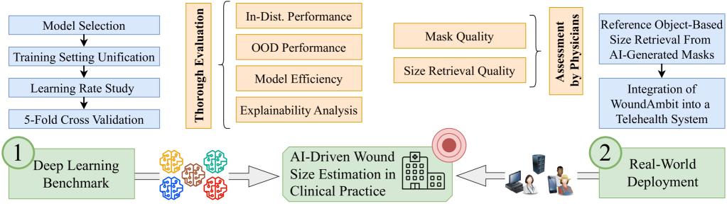
The paper is structured as follows: Section 2 describes the \acdl benchmark (Fig. 1, left), covering model selection, methodology, datasets, and results. Section 3 details the size retrieval process and its evaluation, along with the integration of \acwoundambit into a specially designed telehealth system (Fig. 1, right). Finally, Section 4 discusses key findings, and Section 5 concludes the study.
2 Deep Learning Benchmark
2.1 Model Selection
Given the large number of novel methods introduced in recent years, it is impractical to include all current \acsota models in this study. To ensure a benchmarking process that is as representative and balanced as possible, we devise four categories, selecting several representatives from each of them as follows:
Table 1 summarizes our final selection, striking a balance between domain specificity, cross-domain variety, and methodological diversity. The key ideas of all architectures are briefly summarized in Section A.1, with further details available in the corresponding publications. Overall, our selection process is guided by the following criteria: (I) Architectural diversity: To ensure a comprehensive representation of various design paradigms, we aim for a balance between \accnn-based, \acvit-based, and hybrid methods. (II) Computational efficiency: Given the limited resources in healthcare settings, we prioritize models that offer a good trade-off between performance and computational feasibility. For \acgp models, we select architectures with approximately 50–60M parameters, while wound-specific and medical models range from 30–70M parameters, mainly due to the limited availability of varied model sizes in these domains. (III) Scientific impact and recognition: We select models with significant visibility in their respective fields, prioritizing those published in high-impact conferences and journals. (IV) Code availability: To minimize the risk of implementation errors, we limit our selection to models with publicly available code.
2.2 Unified Training Procedure: Methodological Details
We establish a unified benchmarking environment by standardizing the training process as follows: To ensure an unbiased comparison while enabling the use of pre-trained weights, the deep learning methods were implemented with their architecture-specific settings, as recommended in their respective official publications and code repositories. Specifically, we use ImageNet-pretrained backbones for all methods. While maintaining key architectural parameters (e.g., layer configurations and activation functions), we standardize other training settings across all models. These include input tensor dimensions, the number of training epochs, early stopping criteria, optimizer type, loss function, and the data augmentation pipeline. Further details on preprocessing, data augmentation, and exact training configurations are provided in Section A.2. To minimize biases associated with fixed learning rates, we conduct a preliminary hyperparameter tuning step for each architecture, optimizing the learning rate within a predefined search range (). The best-performing learning rate for each method (see Section A.2) is then used for subsequent five-fold \accv, while all other training settings remained unified. Overall, this ensures that performance differences arise from the intrinsic capabilities of the architectures rather than variations in training configurations, particularly data augmentation.
2.3 Standardized Evaluation Procedure
Our assessment strategy employs a unified evaluation framework, incorporating both traditional segmentation metrics and practical aspects essential for clinical applications. For segmentation performance, we use metrics such as mean Intersection over Union (mIoU), Dice Similarity Coefficient (mDSC), precision (mPrc), and recall (mRec). These metrics evaluate performance on both our main dataset and unseen \acood data, with the latter specifically assessing the generalization capability across diverse wound types. In terms of model efficiency, we report the number of trainable parameters and \acpgmac, along with mean inference time for GPU and CPU execution and throughput in images per second (IPS). Finally, we assess explainability using \acgradcam-based visualizations. Further information and implementation details are available in Section A.3.
2.4 Datasets
Our experiments mainly rely on two datasets, detailed in Section A.4. The first, CFU, is used for model training, including learning rate studies and final \accv. It consists of a custom combination of the publicly available \acsdfuc22 dataset [13], which contains 2,000 annotated images, and the \acfuseg’21 challenge dataset [30], with 1,010 labeled images. After removing duplicates and highly similar images, 2,887 unique images remain for our experiments. Additionally, we use the \acsdfuc22 test set for external validation of our models via the challenge’s live leaderboard. The second, denoted as out-of-distribution (OOD) dataset, was collected at the University Hospital of Würzburg with approval from the local ethics committee. It comprises 343 expert-annotated wound images from various anatomical sites, extending beyond foot ulcers. To better reflect real-world clinical conditions, where patient-acquired images often lack standardized imaging protocols, certain wounds were intentionally captured multiple times from varying distances, angles, and perspectives. Notably, \acood is used exclusively for evaluation, not for training. Due to privacy regulations, it remains confidential, though selected examples will be shared at GitHub with written consent.
2.5 Performance on CFU Dataset and \acdfuc22 Live Leaderboard
Table 2 presents the 5-fold \accv results on CFU alongside each model’s performance on the \acdfuc22 live leaderboard. For the latter, instead of selecting the best checkpoint from individual folds, segmentation masks are generated using \acppmv across all five instances of each architecture. This approach mitigates overfitting to individual training folds while leveraging the collective strengths of multiple trained instances. The full \accv results are provided in Section A.5. On CFU, \actransnext demonstrated the highest performance, achieving an mIoU of 79.8 and an mDSC of 88.7. \acsegnext followed closely with an mIoU of 79.5 and an mDSC of 88.6, exhibiting strong consistency across the \accv folds. On the \acdfuc22 leaderboard, \actransnext also achieved the highest performance among our models, with an mIoU of 62.8 and an mDSC of 73.0, slightly surpassing \acsegnext and \acvwconv — the latter ranking third despite its moderate performance on CFU. Notably, \actransnext ranked 6th out of 60 (top 10%) based on the best submission per participant - despite no dataset-specific optimization, which highlights its strong out-of-the-box performance. In contrast, \acunet and most medical approaches, except \acfcbformer, showed worse segmentation performance, ranking lower on both CFU and \acdfuc22.
Type Avg. CFU \acdfuc22 mIoU mDSC mPrc mRec mIoU mDSC \actransnext 79.8±1.4 88.7±0.8 90.9±0.4 86.7±1.8 62.8 73.0 \acsegnext 79.5±0.7 88.6±0.4 90.7±0.6 86.6±0.6 62.1 72.3 \acsegformer 78.9±0.8 88.2±0.5 90.4±0.7 86.1±1.4 61.8 72.1 \acfcbformer 78.6±1.5 88.0±0.9 90.6±0.6 85.6±1.9 62.0 72.2 \acinternimage 78.5±0.9 88.0±0.5 89.8±1.5 86.2±0.6 61.7 72.0 \acsvwmit 78.5±1.7 87.9±1.0 90.2±1.1 85.8±2.2 61.7 72.0 \acvwconv 78.4±0.5 87.9±0.3 90.1±1.9 85.9±2.0 62.0 72.3 \acfusegnet 78.0±1.3 87.6±0.8 90.6±0.7 84.9±1.3 61.3 71.6 \achardnet 76.9±1.4 86.9±0.9 88.3±2.4 85.8±2.5 60.4 70.8 \acunet 74.1±0.9 85.1±0.6 88.1±1.1 82.5±1.5 57.6 68.0 \acmissformer 70.0±2.7 82.3±1.8 85.8±3.4 79.3±3.3 55.6 66.4 \achiformer 73.8±1.8 84.9±1.2 87.6±1.6 82.5±1.7 57.7 68.2
2.6 Performance on Out-of-Distribution (OOD) Data
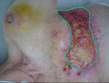
Table 3 presents the segmentation performance on the unseen \acood dataset, which includes previously unobserved anatomical regions, such as the head and breast, thereby assessing model generalization to domain shifts. In addition to reporting the average and standard deviation (SD) across the five \accv models per architecture, we again provide \acpmv results to ensure a more stable and unbiased evaluation. Notably, for all models, the \acpmv performance surpasses the average performance of the best models from individual folds in both mIoU and mDSC, further confirming its robustness. \actransnext demonstrated the strongest generalization, achieving the highest mIoU (79.4) and mDSC (88.5) in the \acpmv setting, followed closely by \acinternimage (mIoU 78.8, mDSC 88.1) and \acvwmit (mIoU 78.0, mDSC 87.6). The performance drop relative to the in-distribution CFU data was minimal (0.5pp mIoU, 0.3pp mDSC) for the top three models. \acinternimage even showed a 0.3pp improvement in mIoU, indicating strong adaptability to novel wound types. \acsegformer, \acvwconv, and \achardnet also maintained competitive performance relative to CFU (1pp mIoU drop). \acfcbformer achieved the highest absolute \acpmv scores among the medical architectures (mIoU 76.5, mDSC 86.7). In contrast, the remaining medical models, except for \achardnet, exhibited substantial performance declines (4–7.9pp mIoU), with \achiformer dropping below 68% mIoU. Notably, \acsegnext, despite its strong in-distribution and \acdfuc22 performance, saw a sharp decline of 3.7pp in mIoU.
Type Avg. CFU Avg. OOD Maj. vote OOD mIoU mDSC mIoU mDSC mPrc mRec mIoU mDSC mPrc mRec \actransnext 79.8 88.7 78.3±1.7 87.8±1.1 93.6±0.2 82.7±1.9 79.4 88.5 94.3 83.4 \acinternimage 78.5 88.0 76.0±3.2 86.3±2.1 92.4±0.6 81.1±3.6 78.8 88.1 93.7 83.2 \acvwmit 78.5 87.9 75.7±1.6 86.2±1.0 92.8±0.5 80.5±2.0 78.0 87.6 93.7 82.3 \acsegformer 78.9 88.2 76.3±1.2 86.5±0.7 93.1±0.6 80.8±1.4 77.7 87.5 94.1 81.7 \acvwconv 78.4 87.9 74.9±2.7 85.7±1.8 93.1±0.8 79.4±3.5 77.2 87.1 94.4 80.9 \acfcbformer 78.6 88.0 74.0±1.9 85.1±1.3 93.2±1.0 78.3±2.7 76.5 86.7 94.5 80.0 \achardnet 76.9 86.9 73.0±2.6 84.4±1.7 91.1±2.1 78.7±4.1 75.9 86.3 93.1 80.4 \acsegnext 79.5 88.6 74.5±1.7 85.4±1.1 93.4±0.3 78.6±2.0 75.8 86.2 94.4 79.4 \acfusegnet 78.0 87.6 71.5±3.2 83.4±2.2 94.2±0.8 74.9±3.9 74.0 85.1 95.7 76.5 \acunet 74.1 85.1 65.6±2.7 79.2±2.0 91.9±0.6 69.7±3.3 67.5 80.6 93.3 70.9 \acmissformer 70.0 82.3 64.3±2.6 78.2±2.0 88.7±1.6 70.1±3.5 66.0 79.5 90.2 71.1 \achiformer 73.8 84.9 63.1±5.1 77.3±3.9 90.8±2.0 67.7±6.3 65.9 79.4 92.4 69.6
2.7 Model Efficiency Analysis
We report key computational metrics in Table 4. Among all architectures, \acfusegnet has the highest number of trainable parameters (71M), while \achiformer and \acunet are the smallest. In terms of \acpgmac, \acmissformer is the most efficient, whereas \acunet, and, especially, \actransnext and \acinternimage exhibit higher computational complexity. Interestingly, parameter count and GMACs do not always directly correspond to inference time and throughput (TP). For instance, despite having similar parameter counts to most models (50–60M), \actransnext and \acfcbformer exhibit considerably higher inference times and lower TP, making them the slowest on both GPU and CPU. In contrast, \acunet, despite having the third highest GMAC count, achieves the fastest GPU inference time, highlighting the influence of architectural design and optimizations on computational efficiency. The results reveal a trade-off between efficiency and segmentation performance. While models such as \acunet, \acmissformer, and \achiformer excel in inference speed on both GPU and CPU, advanced vision models like \actransnext and \acinternimage offer superior segmentation performance at a moderate computational cost. Notably, even \actransnext, the slowest model, maintains a throughput of approximately one IPS on the CPU and up to 24 IPS on the GPU.
Type OOD Params GMACs Inference Time ± SD (in ms) TP (in IPS) mIoU (in M) GPU CPU GPU CPU \actransnext 79.4 57.74 238.41 41.58 ± 0.10 1012.75 ± 243.11 24.05 0.99 \acinternimage 78.8 58.37 234.23 28.71 ± 0.29 692.35 ± 42.90 34.83 1.44 \acvwmit 78.0 51.42 62.79 25.65 ± 0.11 439.98 ± 55.75 38.98 2.27 \acsegformer 77.7 47.22 71.18 23.54 ± 0.08 429.89 ± 17.95 42.48 2.33 \acvwconv 77.2 57.00 77.43 25.55 ± 0.03 339.08 ± 38.59 39.13 2.95 \acfcbformer 76.5 52.96 149.93 51.27 ± 0.09 875.13 ± 41.01 19.51 1.14 \achardnet 75.9 51.06 138.92 38.01 ± 0.16 669.29 ± 17.98 26.31 1.49 \acsegnext 75.8 48.77 64.18 29.50 ± 0.42 616.49 ± 59.53 33.90 1.62 \acfusegnet 74.0 70.97 35.51 32.99 ± 0.13 526.02 ± 69.17 30.31 1.90 \acunet 67.5 31.03 192.67 13.79 ± 0.02 307.96 ± 15.82 72.50 3.25 \acmissformer 66.0 42.46 7.16 17.78 ± 0.15 203.07 ± 19.05 56.24 4.92 \achiformer 65.9 25.51 11.51 14.09 ± 0.13 251.57 ± 19.80 70.96 3.98
2.7.1 Explainability Insights
To assess the decision-making of our models, we applied \acgradcam to generate visual explanations of predictions. Figure 2 presents visualizations for the top three and two lowest-performing models from Table 3, along with the predicted segmentation masks (red) for selected OOD images. Additional comparisons across architectures and further examples of different body localization, wound size, and color variations are provided in Section A.6.
1 2 3 4 5 6 7 8 9 10 11 12
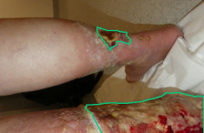
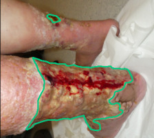
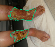
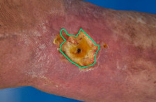
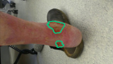
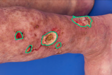
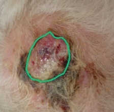
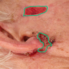
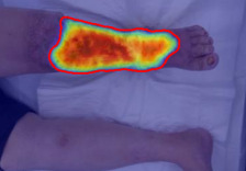
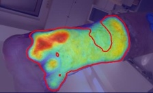
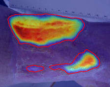
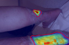
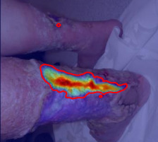
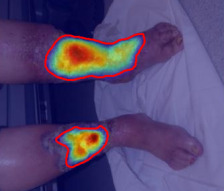
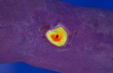
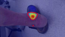
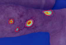
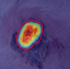
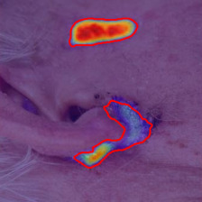
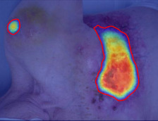
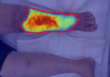
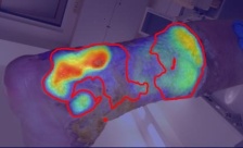
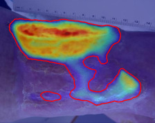
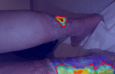
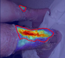
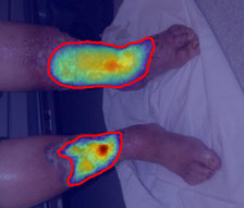
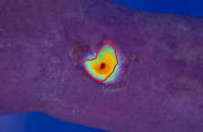

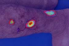
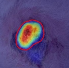
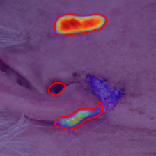
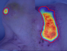
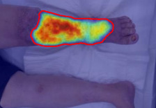
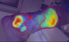
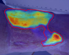
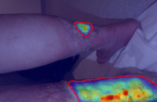
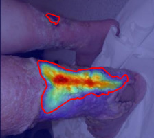
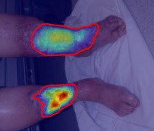
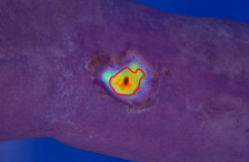
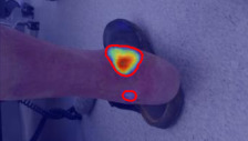
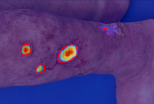
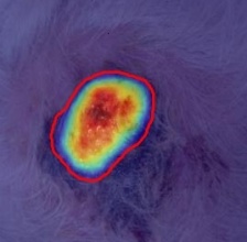
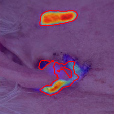
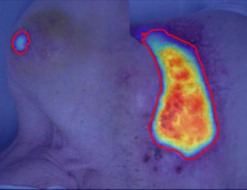
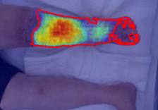
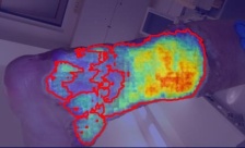
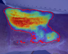
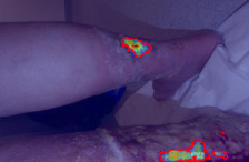
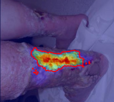
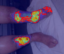
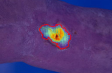
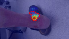
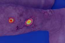
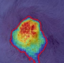
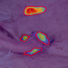
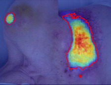
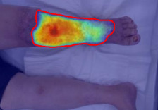
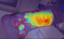
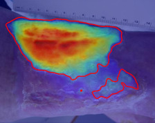
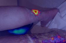
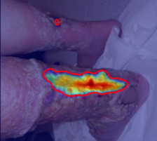
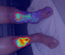
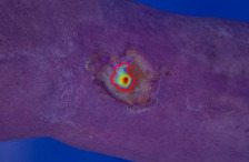
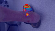
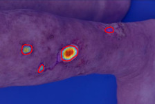
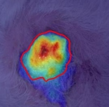
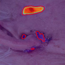
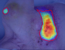
By comparing heatmaps with \acgt masks (green), we qualitatively assess model reliability, focusing on whether activations align with clinically relevant wound features rather than artifacts. Across all models, strong activations were frequently observed in wound regions, aligning well with \acgt masks. Additionally, non-wound regions often exhibited minimal to no activation, suggesting effective prioritization of pathological features. Qualitative comparisons indicate that higher-performing models from Table 3 tend to generate sharper heatmap boundaries and achieve more precise wound localization, whereas lower-performing models exhibit weaker or more diffuse activations (3, 7). In some cases, non-wound objects (e.g., shoes, 5) were misidentified as wounds, while certain wound regions (6, 7, 8), including those near image edges (9), were not fully captured, especially by lower-performing models. Additionally, weaker models occasionally generated pixelated or irregular mask predictions, as indicated by frayed or poorly defined red contours (7, 11, 12). While not being necessarily generalizable, this qualitative insights align with quantitative performance metrics and enhances interpretability for clinicians, allowing for a deeper understanding of model behavior and fostering greater trust in AI systems.
3 Real-World Deployment
3.1 Automated Size Retrieval from AI-Generated Masks
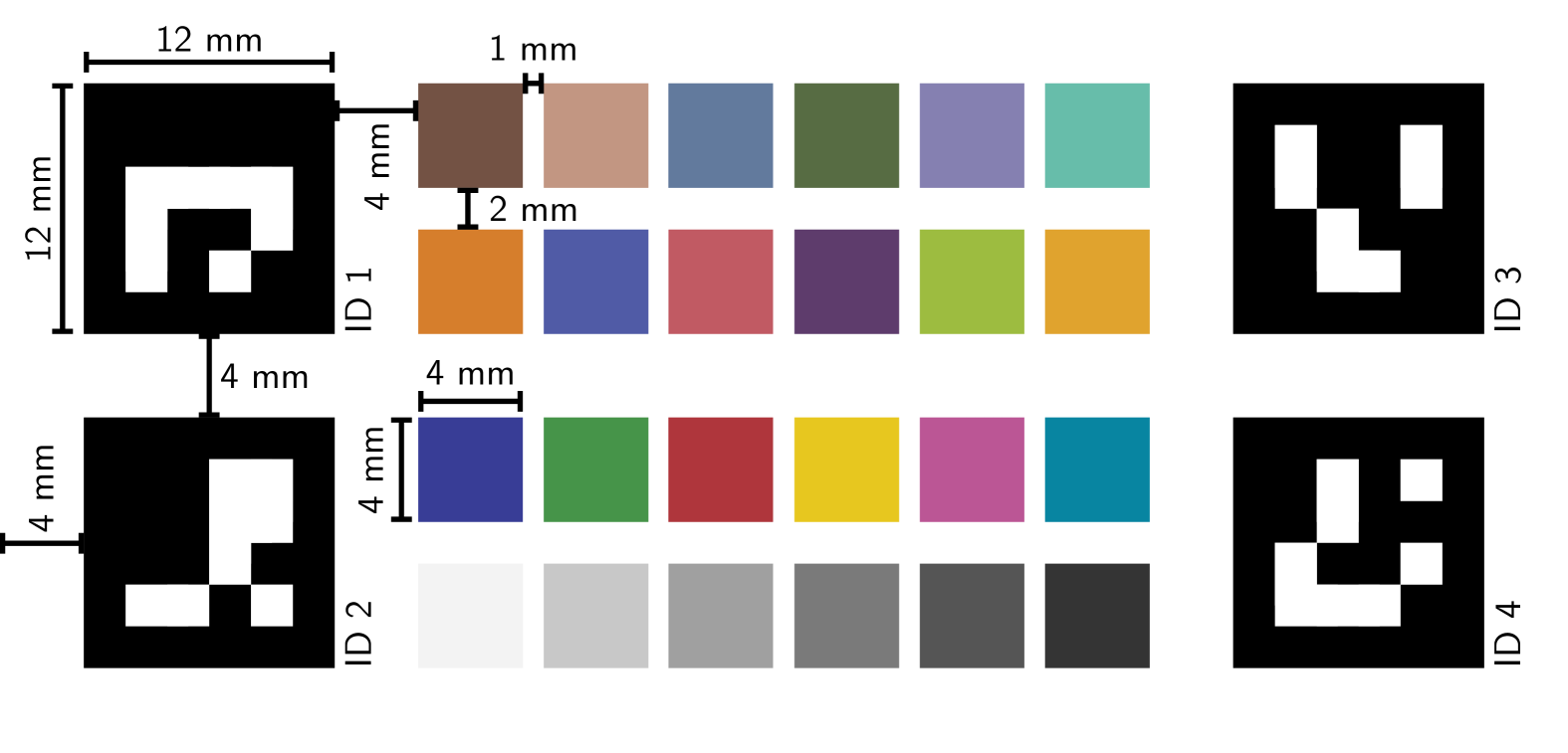
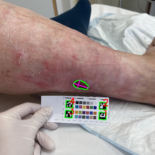
Reference Object (RO) Design. Based on Chairat et al. [3], we developed a custom \acro with slight adjustments to size and layout (see Fig. 3(a)). Our \acro is placed next to the wound and features four \acaruco markers, each with a 12 mm side length and a 4 mm margin of white space to facilitate accurate detection. To enhance functionality, we included a Macbeth color chart with 24 color patches between the markers, aligned such that the top and bottom edges of the patch groups align with the marker corners to simplify automated extraction.
Benefits. Unlike existing methods [4, 6], our \acaruco-based \acro, with its known dimensions, enables precise object size estimation independent of AI algorithms. Notably, this approach removes the necessity of including \acro detection as an additional class in model training. For future applications, the Macbeth color chart enables color calibration and wound color assessment. In environments with few natural reference points (e.g., human skin), the fixed design helps estimate camera position and rotation, which could be used for real-time patient guidance during image capture (e.g., adjusting distance or angle).
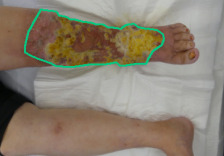
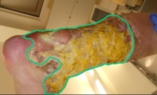
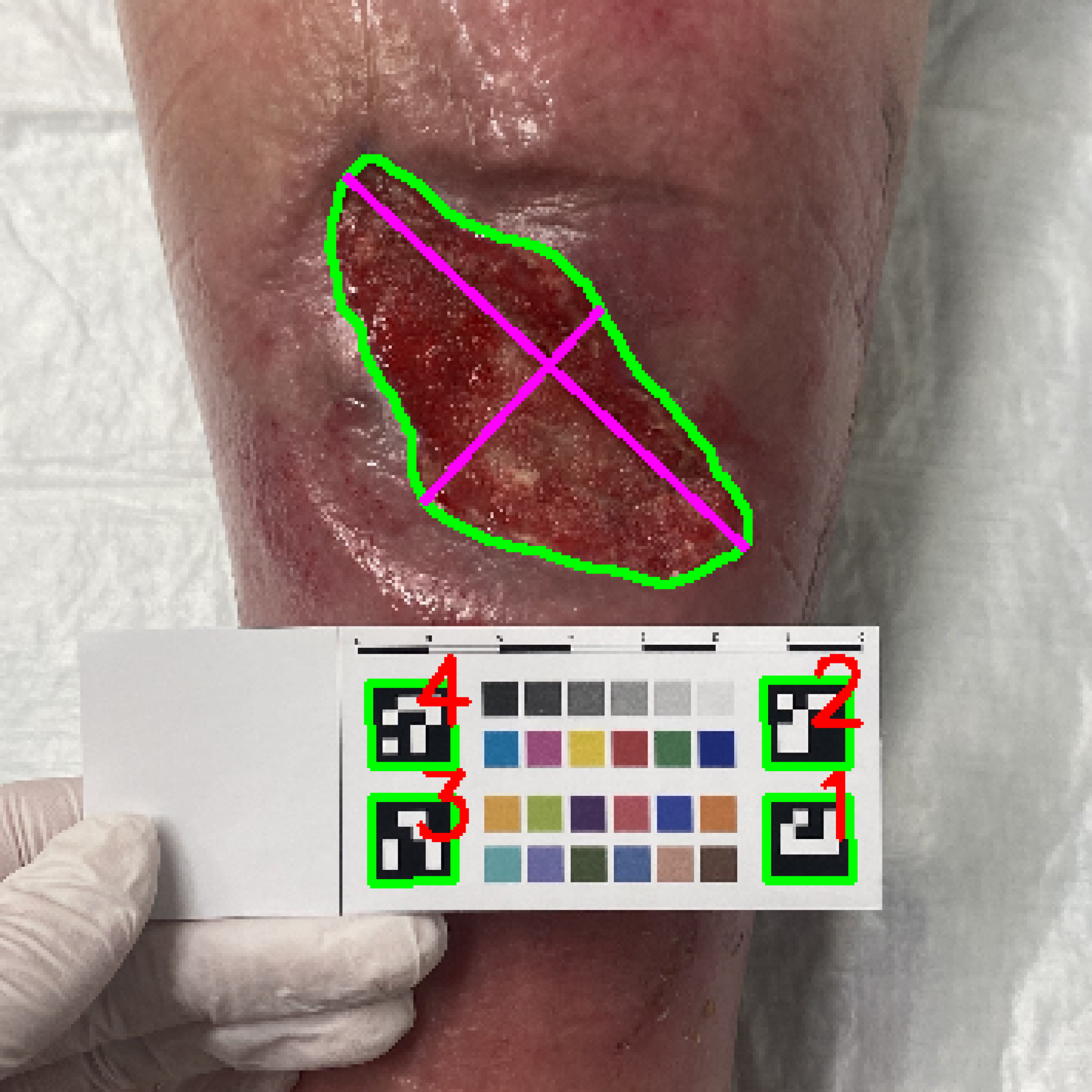
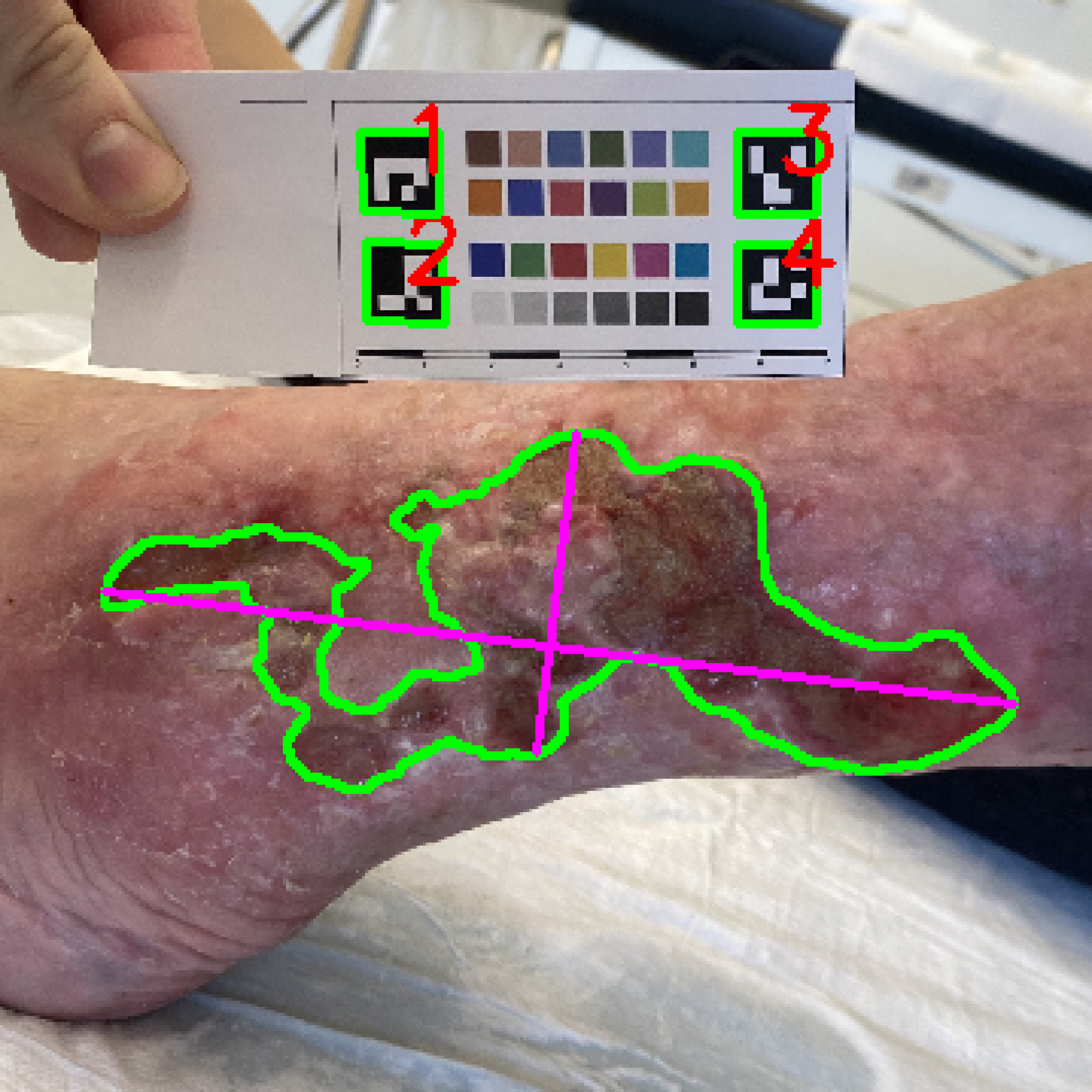
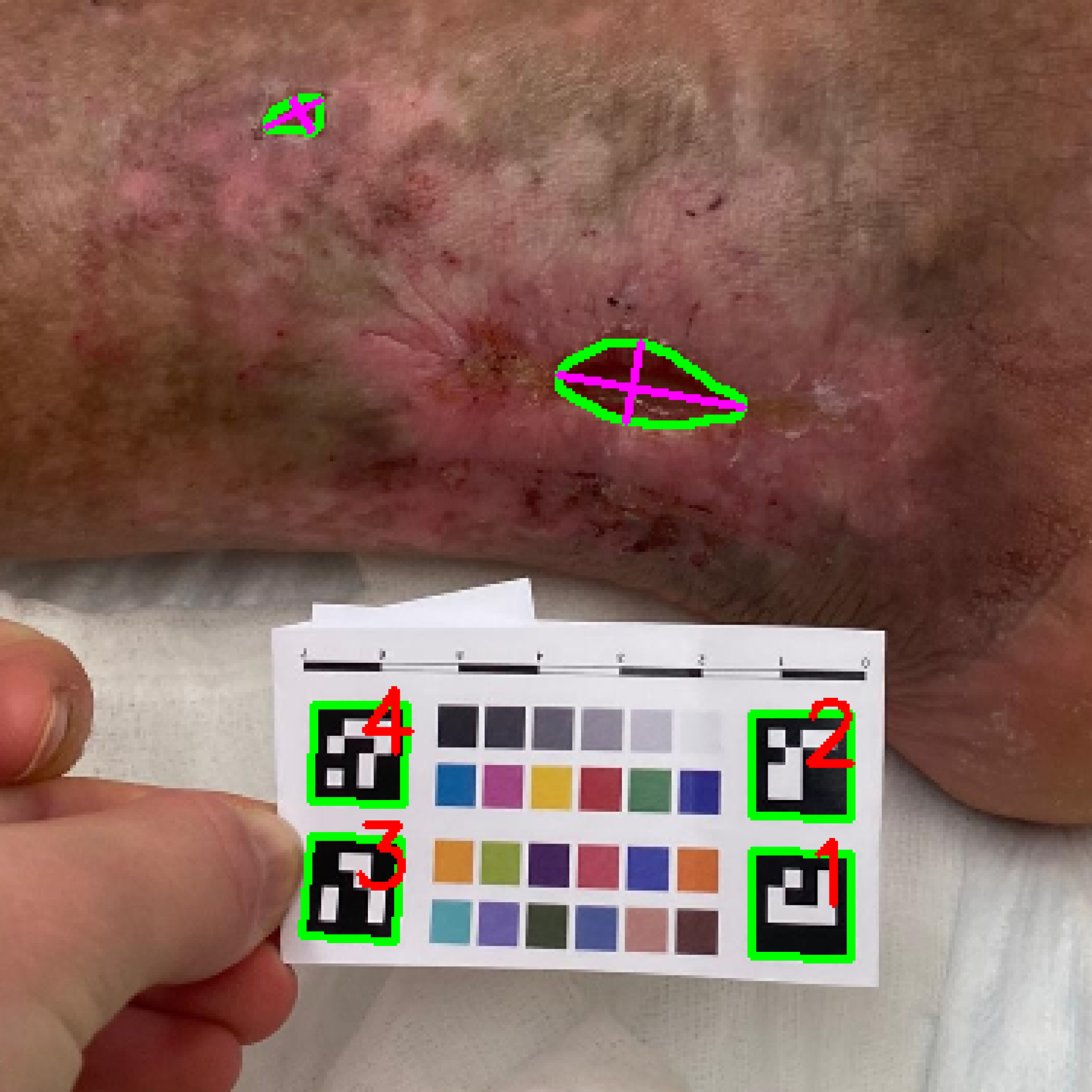
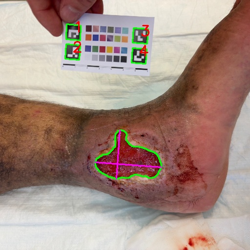
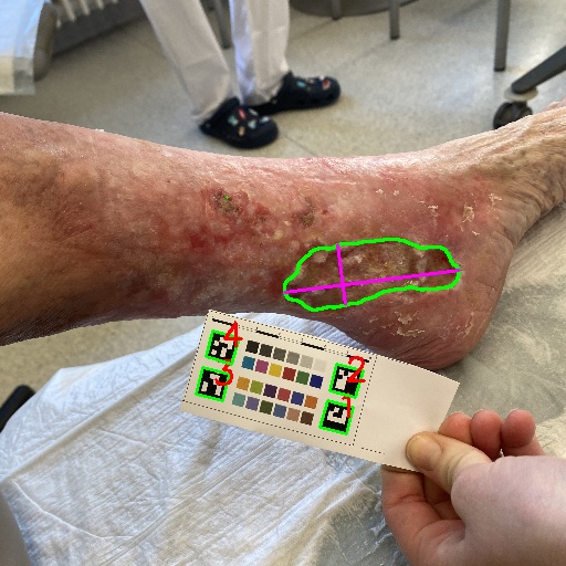
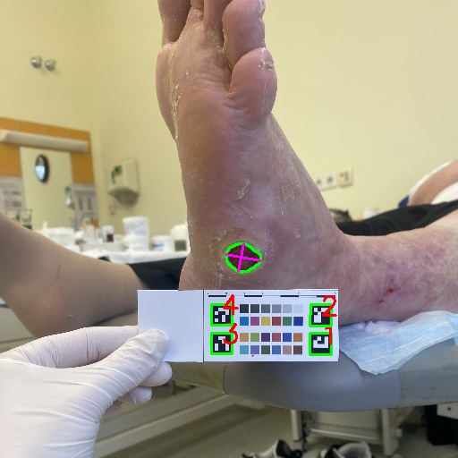
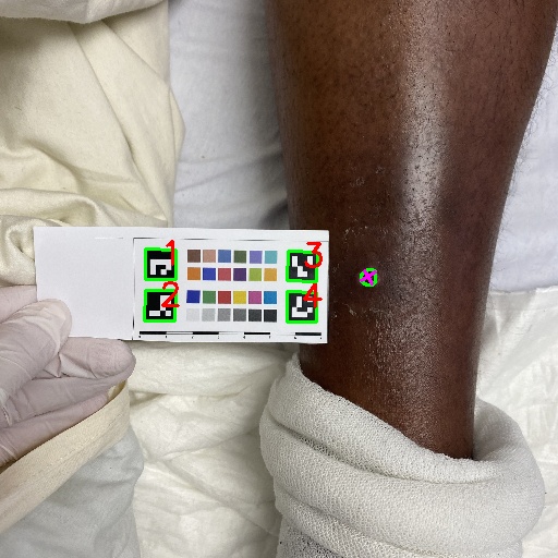
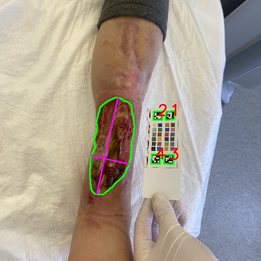
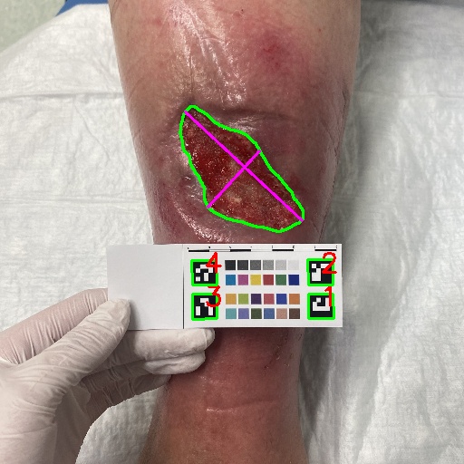
Size Retrieval Process. First, we detect the \acaruco markers using OpenCV’s ArucoDetector. To estimate the pixel-to-millimeter (px/mm) ratio, we design a robust approach that utilizes multiple \acaruco markers whenever possible, computing the ratio using predefined real-world distances between specific marker pairs. By calculating the mean px/mm ratio across all available pairs, we reduce the impact of perspective distortion and measurement noise. Moreover, this approach allows for a more stable estimation, even in cases where some markers are partially occluded or missing. If only one marker is detected, we estimate the px/mm ratio by averaging its width and height. Afterwards, we convert segmented wound areas into square millimeters using this ratio. In addition, we determine the wound’s height and width following standard clinical measurement practices [19]. We identify the longest diagonal of each mask contour (with at least seven points). Then, a perpendicular vector is computed and moved incrementally along the diagonal. At each step, we measure the distance between intersections of the perpendicular line and the contour, selecting the two points with the greatest separation to define the second diagonal, representing wound width. Figure 3 demonstrates the size retrieval process for three representative patients. Green contours indicate detected markers and wound regions, while pink lines represent the diagonals approximating wound height and width. Red numbers show the retrieved marker IDs. Notably, accurate wound size estimation requires the \acro to be placed as close as possible to the wound and, crucially, within the same plane to minimize distortion. In contrast, Subfigure 3(c) shows a failure case where the wound is identified correctly, but its size is underestimated due to the markers being positioned closer to the camera than the wound.
Evaluation. To evaluate performance, we collect diverse wound images using our \acro and an iPhone 11. The top five methods, selected based on \acpmv mIoU scores from the OOD dataset, are assessed on these images using \acppmv per architecture. Additionally, an ensemble of all models is constructed. For qualitative evaluation, dermatologists independently review AI-generated masks. A total of image-mask pairs () are presented in random order, with each mask rated as either “good” or “bad”. Physicians also estimate wound sizes and select the best mask per image. Figure B.1 provides screenshots of the annotation tool. We define the following for evaluation: The Clinical Mask Approval (CMA) measures how often physicians rate the masks as “good” across all images and evaluators. The Expert Choice Rate (ECR) quantifies the proportion, averaged across all images and dermatologists, where a model’s mask is selected as the best of six for a given image.
|
|
(1) |
|
|
(2) |
Since physicians provide separate height and width estimates instead of direct area measurements, we use these as proxies for size estimation accuracy. The \acgt height and width for image are defined as the mean of all physician estimates, denoted as and . To assess size retrieval quality, we employ the Mean Absolute Error (MAE) and Mean Absolute Percentage Error (MAPE). For each dimension , these metrics quantify the deviation between model predictions and the expert-derived GT :
|
|
(3) |
|
|
(4) |
However, size estimation in medical imaging is inherently subjective, leading to significant variability among physicians [12]. To ensure a meaningful evaluation, we quantify inter-rater variability using a relative deviation metric. We exclude any image where the following deviation exceeds a threshold of 0.5 in either height or width annotations, with representing the dimension, and denoting the size annotation provided by physician for image :
|
|
(5) |
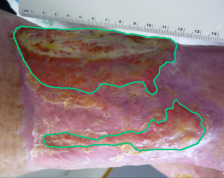
After removing inconsistently annotated images, we use the remaining seven for error calculations (see Table 5). Figure 4 confirms their variability in wound shape, size, and skin tone, ensuring a representative subset for size retrieval evaluation. We also report the mean predicted height and width (MPH, MPW) with SD across the images, alongside the average wound dimensions estimated by the physicians. This analyzes model consistency across wound types and retrieval capabilities relative to expert estimates. For completeness, Table B.1 includes the masks, raw size predictions (including area), and expert estimates for all 20 images, which will be shared at GitHub with written consent.
The CMA ranged from 83.3% to 86.7% across models , reflecting high mask quality and strong physician approval. ECR varied notably, with \acvwconv achieving the highest approval rate (35.0%) and \actransnext and the Ensemble the lowest (8.3%). For size retrieval, all models performed similarly, with MPH and MPW closely aligning with the \acgt. On average, height estimates were slightly overestimated, while width was slightly underestimated. Nevertheless, consistently low MAE (4.4 mm height, 3.2 mm width) and MAPE (14.1% height, 16.2% width) indicate robust size retrieval across wound sizes.
Model Mask Quality Size Retrieval Quality () () Height Width CMA1 ECR1 MPH 2,3 MAE2 MAPE1 MPW 2,4 MAE2 MAPE1 \actransnext 85.0 8.3 54.6 ± 41.0 4.4 12.3 27.2 ± 15.6 3.2 15.8 \acinternimage 86.7 15.0 54.9 ± 40.9 3.9 12.2 26.6 ± 15.0 3.2 16.2 \acvwmit 86.7 13.3 55.4 ± 41.5 4.3 14.1 27.7 ± 16.0 2.3 13.3 \acsegformer 83.3 13.3 54.8 ± 41.2 3.8 12.0 27.1 ± 15.8 2.6 13.2 \acvwconv 85.0 35.0 54.8 ± 41.6 4.0 9.9 26.6 ± 15.8 3.2 14.4 Ensemble 86.7 8.3 55.0 ± 41.3 4.1 12.2 27.0 ± 15.7 2.9 15.1 1 In % 2 In mm 3 Mean : 54.3 ± 41.6 4 Mean : 29.2 ± 16.3
3.2 Seamless Integration into a Custom Telehealth System
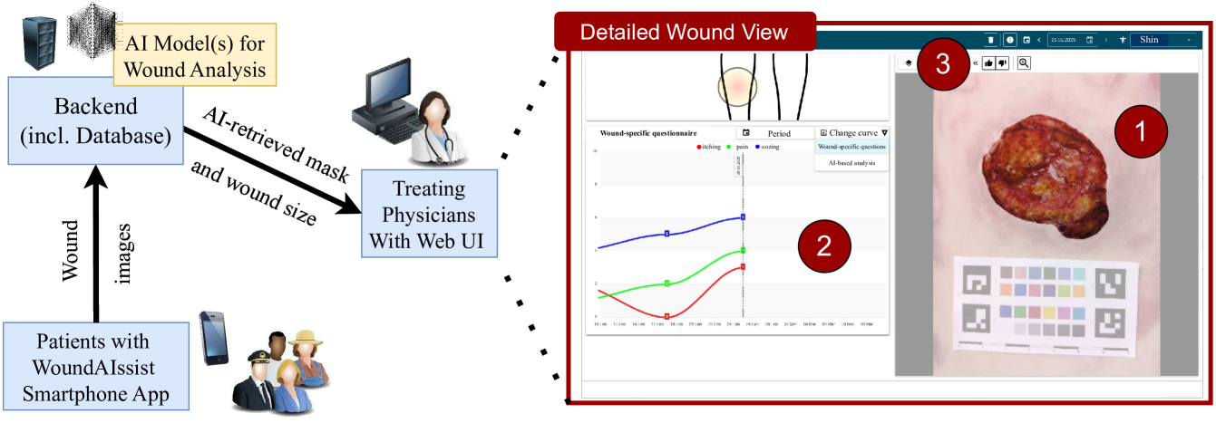
We integrate the AI module, which demonstrated superior performance in terms of ECR, \acvwconv, and wound size retrieval, into a custom-developed telehealth platform to enable future evaluation of its impact on patient outcomes. The system architecture (see Figure 5) consists of three core components: (1) the WoundAIssist mobile application (2) a web interface for physicians, and (3) a backend with a dedicated microservice for AI processing. Among other features, patients use our purpose-built app, WoundAIssist, to capture and upload wound images at regular intervals, accompanied by self-reported data on wound-specific factors (e.g., pain, itching, oozing) and overall well-being (e.g., mood, activity impact, quality of life). \achcp use a web-based dashboard for remote patient monitoring, providing a concise summary of essential patient information. The dashboard also includes a detailed wound view (Fig. 5, right, translated), which displays the selected wound images alongside the AI-predicted wound area (\raisebox{-0.9pt}{1}⃝). Additionally, the dashboard features trajectory curves for all patient-reported wound scores and AI-derived wound size progression (\raisebox{-0.9pt}{2}⃝). To support continuous model refinement, the system incorporates a feedback mechanism, allowing clinicians to assess the segmentation masks by a simple approval process (\raisebox{-0.9pt}{3}⃝).
4 Discussion and Outlook
This study provides a comprehensive benchmark of various \acdl models for wound segmentation, addressing real-world challenges in clinical deployment and telehealth applications. Although no clear trend emerged between CNN- and ViT-based models, the results from both the in-distribution CFU and the \acdfuc22 live leaderboard indicate the superior performance of modern \acgp architectures, such as \actransnext, over specialized medical models. Similarly, the top five models on the \acood dataset were \acgp architectures, further emphasizing the superiority of contemporary SS and vision models over specialized medical techniques in handling OOD data. This enhanced performance is further supported by visual analysis of Grad-CAM heatmaps. Despite the higher computational demands of the top-performing models, inference times remained within practical limits. With a minimum throughput of at least one image per second on the CPU, all models are considered suitable for clinical use and remote wound size monitoring, given the manageable data volumes. Expert evaluations of mask quality and automated size estimates from the top five models yielded promising results, with high mask approval rates and size estimates closely aligning with dermatologist annotations. While no architecture clearly outperformed the others in size retrieval, \acvwconv was most favored by experts for best mask selection.
Even tough our proposed wound size estimation framework, \acwoundambit, holds great potential, this study has some limitations: The evaluation primarily used publicly available and \acood images captured in controlled hospital settings. To improve model robustness and assess size estimation in telemedicine, it is essential to include images from home environments, particularly those taken by patients using smartphones. Additionally, further analysis is needed to evaluate size estimation accuracy when not all markers are detected; only one of the 20 images used had partly occluded markers. While efforts were made to select a representative set of models, the evaluation is constrained by the chosen architectures. The three lowest-performing models –\acunet, \acmissformer, and \achiformer– are notably smaller in terms of parameters, potentially introducing a slight bias. However, the general trend favoring GP SS and vision models remains consistent, even regarding the larger medical networks. Regarding patient well-being, \acwoundambit serves as a decision support system, not a replacement for physicians. The AI component tracks wound size automatically, but dermatologists still review both the raw image and AI output, ensuring clinical decisions are not based solely on AI predictions. Nevertheless, the potential risk of over-reliance on technology should be further explored in future studies. Overall, clinical validation of \acwoundambit is crucial to confirm its effectiveness in practice.
5 Conclusion
This work advances automated wound segmentation by benchmarking 12 \acsota \acdl methods from \acgp vision, medical segmentation, and wound care. We address challenges such as domain variability, computational constraints, and model interpretability. Our evaluation on both in-distribution and \acood datasets demonstrates that modern GP models, especially \actransnext and \acvwformer, exhibit strong generalization and remain computationally feasible for clinical use. While our AI-driven wound size estimation framework, \acwoundambit, shows strong clinical promise, future work will focus on expanding the dataset with smartphone images from diverse patient demographics and conditions for model finetuning. Additionally, integrating \acwoundambit with existing clinical systems and assessing patient-reported outcomes in clinical trials will be crucial for evaluating its real-world impact. Lastly. incorporating the \acood dataset and prospectively collected smartphone images into training is expected to further improve model performance. In summary, this work represents an important step toward bridging recent advances in computer vision with real-world wound care, offering the potential to improve remote wound size monitoring and enhance patient care.
5.0.1 Acknowledgements
We would like to express our gratitude to Luisa Deutzmann for her assistance in creating the dataset of 20 images for size retrieval evaluation. We also wish to thank Caroline Glatzel for her contribution to the manual size annotation of these images and the evaluation of the AI-generated wound masks.
5.0.2 Ethics
The authors declare no conflicts of interest. Ethical approval for this study was waived by the Ethics Committee of the Medical Faculty of the University of Würzburg. All patients provided informed consent for the publication of their photographs.
References
- [1] Awais, M., et al.: Foundation models defining a new era in vision: a survey and outlook. IEEE TPAMI (2025)
- [2] Azad, R., et al.: Advances in medical image analysis with vision transformers: a comprehensive review. Med. Image Anal. (2024)
- [3] Chairat, S., et al.: Ai-assisted assessment of wound tissue with automatic color and measurement calibration on images taken with a smartphone. Healthcare (2023)
- [4] Chino, D.Y., et al.: Segmenting skin ulcers and measuring the wound area using deep convolutional networks. Comput. Methods Programs Biomed. (2020)
- [5] Dhar, M., et al.: Fusegnet: A deep convolutional neural network for foot ulcer segmentation. Biomed. Signal Process. Control (2024)
- [6] Foltynski, P., Ladyzynski, P.: Internet service for wound area measurement using digital planimetry with adaptive calibration and image segmentation with deep convolutional neural networks. Biocybern. Biomed. Eng. (2023)
- [7] Goyal, M., et al.: FCNs for diabetic foot ulcer segmentation. In: SMC (2017)
- [8] Guo, M.H., et al.: Segnext: Rethinking convolutional attention design for semantic segmentation. NeurIPS (2022)
- [9] Heidari, M., other: Hiformer: Hierarchical multi-scale representations using transformers for medical image segmentation. In: WACV (2023)
- [10] Huang, X., et al.: Missformer: An effective transformer for 2d medical image segmentation. IEEE T-MI (2023)
- [11] imito AG: imitoWound (2025), https://imito.io/en/imitowound
- [12] Jørgensen, L.B., et al.: Methods to assess area and volume of wounds–a systematic review. Int Wound J (2016)
- [13] Kendrick, C., et al.: Translating clinical delineation of diabetic foot ulcers into machine interpretable segmentation. arXiv (2022)
- [14] Kirillov, A., et al.: Segment anything. In: ICCV (2023)
- [15] Liao, T.Y., et al.: Hardnet-dfus: Enhancing backbone and decoder of hardnet-mseg for diabetic foot ulcer image segmentation. In: DFU Grand Challenge (2022)
- [16] Liu, X.a.: A framework of wound segmentation based on deep convolutional networks. In: CISP-BMEI (2017)
- [17] Ma, J., et al.: Segment anything in medical images. Nat. Commun. (2024)
- [18] Minaee, S., et al.: Image segmentation using DL: A survey. IEEE TPAMI (2021)
- [19] Nichols, E.: Wound assessment part 1: how to measure a wound. Wound Ess. (2015)
- [20] Oota, S.R., et al.: Wsnet: towards an effective method for wound image segmentation. In: WACV (2023)
- [21] Peterson, N., et al.: Size matters: how accurate is clinical estimation of traumatic wound size? Injury (2014)
- [22] Ramachandram, D., et al.: Fully automated wound tissue segmentation using deep learning on mobile devices: cohort study. JMIR Mhealth Uhealth (2022)
- [23] Rayed, M.E., et al.: Deep learning for medical image segmentation: State-of-the-art advancements and challenges. IMU (2024)
- [24] Ronneberger, O., et al.: U-net: Convolutional networks for biomedical image segmentation. In: MICCAI (2015)
- [25] Sanderson, E., Matuszewski, B.J.: Fcn-transformer feature fusion for polyp segmentation. In: MIUA (2022)
- [26] Shi, D.: Transnext: Robust foveal visual perception for ViTs. In: CVPR (2024)
- [27] Siddique, N., et al.: U-net and its variants for medical image segmentation: A review of theory and applications. IEEE Access (2021)
- [28] Thisanke, H., et al.: Semantic segmentation using vision transformers: A survey. Eng. Appl. Artif. Intell. (2023)
- [29] Wang, C., et al.: Fully automatic wound segmentation with deep convolutional neural networks. Sci. Rep. (2020)
- [30] Wang, C., et al.: Fuseg: The foot ulcer segmentation challenge. Information (2024)
- [31] Wang, L., et al.: Area determination of diabetic foot ulcer images using a cascaded two-stage svm-based classification. IEEE TBME (2016)
- [32] Wang, W., et al.: Internimage: Exploring large-scale vision foundation models with deformable convolutions. In: CVPR (2023)
- [33] Xiao, T., et al.: Unified percept. parsing for scene understanding. In: ECCV (2018)
- [34] Xie, E.a.: Segformer: Simple and efficient design for semantic segmentation with transformers. NeurIPS (2021)
- [35] Yan, H., et al.: Multi-scale representations by varying window attention for semantic segmentation. In: ICLR (2024)
- [36] Zhang, P., et al.: Interactive skin wound segmentation based on feature augment networks. IEEE J-BHI (2023)
- [37] Zhang, R., et al.: A survey of wound image analysis using deep learning: classification, detection, and segmentation. IEEE Access (2022)
WoundAmbit: Bridging State-of-the-Art Semantic Segmentation and Real-World Wound Care
- Supplementary Material -
Vanessa Borst (✉)Timo Dittus Tassilo Dege
Astrid Schmieder Samuel Kounev
Appendix 0.A Deep Learning Benchmark
0.A.1 Architecture-Specific Details and Deviations
As mentioned in the main paper, all architectures are implemented with their architecture-specific settings, as recommended in their respective official publications and code repositories.
However, for the sake of completeness, we briefly detail the core ideas and some architecture-specific remarks below:
hardnet \citesuppappendix_liao2022hardnet.
\aclhardnet was the winner of the \acsdfuc22 challenge. It uses the HarDNet-MSEG model \citesuppappendix_huang2021hardnet as a basis and enhances the model by modifying each HarDBlock in the encoder with a novel HarDBlockV2 and replacing the receptive field block (RFB) modules in the decoder with that of Lawin Transformer. Moreover, the authors maintain
an exponential moving average of the model weights to dampen weight updates and employ deep supervision to calculate multiple losses from different stages of the network.
fusegnet \citesuppappendix_dhar2024fusegnet.
\acfusegnet achieved the best performance in the \acsfuseg’21 challenge. It employs a pre-trained EfficientNet-b7 encoder, paired with a decoder that incorporates a modified squeeze-and-excitation (SE) attention module, referred to as parallel scSE (P-scSE), for fusion at each stage. This novel attention mechanism combines both additive and max-out spatial and channel SE (scSE).
Notably, we report 71.0M parameters for \acsfusegnet, as measured using the calflops library, for consistency with other methods. In contrast, the original publication reports 64.9M parameters, a value obtained using torchsummary with the same model code.
fcbformer \citesuppappendix_sanderson2022fcbformer.
The \acfcbformer was designed for poly segmentation. Its encoder comprises two branches:
A Pyramid Vision Transformer (PVTv2 in the B3 variant), which follows the SSFormer architecture but incorporates an enhanced local emphasis module within the progressive locality decoder, and a fully convolutional branch. \acfcbformer uses a simple prediction head that takes a full-size tensor formed by concatenating the up-sampled transformer branch (TB) output with the output from the fully convolutional branch (FCB).
hiformer \citesuppappendix_heidari2023hiformer.
\achiformer is a resource-efficient medical segmentation model incorporating a transformer-based encoder. Specifically, its hybrid encoder consists of two hierarchical components: a CNN (ResNet50 by default) and a Swin Transformer, interconnected via a Double-Level Fusion (DLF) module in the skip connections of the encoder-decoder structure to fuse global and local features. The decoder, inspired by Semantic FPN \citesuppappendix_kirillov2019panoptic, integrates multi-scale features into a unified mask representation.
In preliminary experiments, we evaluated both HiFormerB and HiFormerL, selecting HiFormerB for our final benchmark due to its higher mIoU performance on the validation split of our main dataset while maintaining a lower number of trainable parameters.
missformer \citesuppappendix_huang2022missformer.
\acmissformer is a transformer-based encoder-decoder architecture designed for medical image segmentation. It introduces a redesigned ReMix-FFN layer to effectively integrate global information with local context. The hierarchical encoder consists of multiple stages, each incorporating transformer blocks with ReMix-FFN and a patch merging layer for feature extraction. Likewise, the decoder includes transformer blocks with ReMix-FFN and patch expanding layers for upsampling feature maps. A ReMix Transformer Context Bridge is placed between the encoder and decoder to enhance multi-scale feature representation by capturing both local and global correlations.
In their study, the authors report that \acmissformer, when trained from scratch, surpasses state-of-the-art methods pre-trained on ImageNet. We evaluated both training strategies and observed that pre-training still led to improved validation mIoU performance. Additionally, we compared internal input sizes of 224 and 512, selecting 224 for the final benchmark due to comparable validation mIoU performance while considerably reducing resource demands.
segformer \citesuppappendix_xie2021segformer.
The \acsegformer is a transformer-based architecture for semantic segmentation (SS). It features a lightweight decoder composed solely of MLP modules, which generates segmentation maps at one-fourth of the original resolution, subsequently upscaled using bilinear interpolation. The decoder integrates multi-scale features from different levels of a hierarchical, positional-encoding-free transformer encoder, which the authors call Mix Transformer (MiT).
segnext \citesuppappendix_guo2022segnext.
The \acsegnext architecture for SS features a novel Multi-Scale Convolutional Attention Network (MSCAN) as its encoder, and a Hamburger Module \citesuppappendix_geng2021attention as its decoder. The encoder comprises a pyramid structure with MSCA blocks, while the decoder combines features from different encoder stages and applies matrix decompositions to them. More precisely, the Hamburger decoder models the prediction task as a low-rank matrix recovery problem, which allows for higher computational efficiency.
vwformer.
Yan et al. introduced the multi-scale decoder \acvwformer, which leverages varying window attention to enhance multi-scale representations for SS. Their proposed decoder is evaluated with various backbone architectures, including ConvNeXt, Swin Transformer, and the MiT encoder from \acsegformer.
As the corresponding GitHub repository did not provide the exact configurations used for the MiT combination, an exact replication of their settings in our benchmark was not feasible. For our evaluation, we set the nheads parameter to one and enabled the short_cut parameter.
internimage.
\acinternimage is a large-scale CNN-based foundation model, using deformable convolution as core operation.
The basic blocks used in \acinternimage are composed of layer normalization and feed-forward networks similar to transformers, while the stem and downsampling layers follow conventional CNN’s designs.
transnext.
\actransnext integrates aggregated attention and convolutional GLU to establish a novel visual backbone. Convolutional GLU serves as an advanced channel mixer, bridging GLU and traditional SE mechanisms to enable each token to apply channel attention based on its nearest neighbor image features, thereby enhancing local feature modeling and overall model robustness. Aggregated attention, inspired by biological foveal vision and continuous eye movement, introduces a refined attention mechanism to improve feature representation.
0.A.2 Details on the Unified Training Settings
0.A.2.1 Preprocessing and Data Augmentation.
All images were resized to 512×512 pixels and normalized for both training and evaluation. Annotated masks were thresholded to eliminate out-of-class pixels. To improve model robustness, we applied data augmentation to each training sample, including Gaussian blur (kernel size 25, ), random affine transforms (translations , rotations , scaling 75–125%, shear ), and random horizontal/vertical flips (each with 50% probability).
Additionally, photometric distortions were introduced, modifying brightness (87.5–112.5%), contrast (50-150%), saturation (50-150%), and hue (), applied with a 50% probability.
0.A.2.2 Implementation.
All architectures were implemented in Python 3.11 using PyTorch 2.0.1. Model training was performed on a server equipped with two partitioned NVIDIA A100 GPUs, utilizing two 42 GB VRAM and two 21 GB VRAM instances. Training was conducted end-to-end on the CFU dataset using the AdamW optimizer and the Reflected Exponential (REX) \citesuppappendix_chen2022rex learning rate scheduler, with a maximum of 120 epochs for parameter tuning and 200 epochs for cross-validation. Binary cross-entropy (BCE) loss was employed, and a batch size of eight was selected as the largest feasible size across all methods given hardware constraints. A preliminary learning rate search explored , identifying as preferable for most methods based on validation IoU and as yielding superior performance for \acshiformer, \acssegformer, \acssegnext, \acsvwmit, and \acstransnext.
During cross-validation, early stopping was applied with a patience of 20 epochs and a minimum IoU improvement threshold of 0.001 on the validation set, saving the best-performing model weights for final test evaluation. While some architectures may benefit from extended training, we adopted early stopping with a generous patience of 20 epochs to mitigate overfitting and enhance generalization.
0.A.3 Details on the Uniform Evaluation Procedure
Segmentation Performance. We use established metrics, including mean Intersection over Union (mIoU), Dice Similarity Coefficient (mDSC), precision (mPrc), and recall (mRec). The metrics are computed excluding the background class, using micro-averaging, which aggregates pixel counts across all samples within a given subset of the dataset before calculating the metric values.
Generalization. We assess each model’s generalization capability using unseen \acood data. This aspect is particularly critical for remote patient monitoring, where wound images are captured using various mobile devices under diverse environmental conditions.
Model Efficiency. To evaluate model complexity, we report the number of trainable parameters as an indicator of model capacity and computational demands, along with \acpgmac to quantify the arithmetic operations required for a single forward pass. Both metrics are computed using the calflops tool \citesuppappendix_calflops2023.
For efficiency analysis, we measure inference time separately for GPU and CPU execution, alongside throughput in images per second (IPS). Inference times are recorded with a batch size of one, averaged over 3,000 images following a warm-up of 10 images per model. Experiments are conducted on an NVIDIA A100 GPU (40 GB partition) and an AMD EPYC 7763 64-Core CPU. To ensure realistic computational loads, we use actual wound images , randomly sampling 300 images from both our primary and the \acood datasets.
Inference times are measured for each of the five \accv models per architecture, resulting in a total of images.
Explainability. To improve model interpretability, we utilize Grad-CAM-based visualizations to identify the image regions most influential in segmentation decisions. This method provides insights into the decision-making process, allowing us to assess whether the models correctly focus on wound regions while minimizing attention to non-wound areas and background artifacts. Heatmaps are generated using a slightly modified version of the M3d-CAM PyTorch library \citesuppappendix_m3dCAM2020 to integrate it into our framework. We use the layer=’auto’ setting, which automatically selects the last layer suitable for extracting attention maps, and visualize the averaged heatmaps across the five \accv models.
0.A.4 Datasets
CFU.
We conduct experiments using a custom Combined Foot Ulcers (CFU) dataset, created by merging the publicly available Foot Ulcer Segmentation Challenge 2021 (FuSeg)\citesuppappendix_wang2024fuseg and Diabetic Foot Ulcer Challenge 2022 (DFUC 2022)\citesuppappendix_kendrick2022translating,appendix_yap2024diabetic datasets. FuSeg contains 1,210 images (512×512 pixels), while DFUC 2022 includes 4,000 images (640×480 pixels). Due to private test set annotations, we exclude the test sets of both datasets (200 from FuSeg; 2,000 from DFUC 2022). Moreover, we remove duplicates, identifying them as such by checking for identical raw bytes or using perceptual hashing with a Hamming distance of . After eliminating 123 redundant image-mask pairs, the final CFU dataset comprises 2,887 unique foot ulcer samples.
For our experiments, CFU is randomly split into training (60%), validation (20%), and test (20%) sets for the learning rate study, and into five equally sized folds for \accv.
DFUC’22 Test Set.
To externally validate our models, we submit predictions for 2,000 test images to the challenge’s leaderboard, ensuring standardized evaluation. This is done once, without optimization for leaderboard metrics.
Out-of-Distribution Dataset (OOD). Our OOD dataset was collected at the University Hospital of Würzburg, following approval from the local ethics committee. Most images have a resolution of pixels. They include a diverse range of chronic wounds from various body locations, and thus, extend beyond \acdfu. A total of 343 images were manually annotated by dermatologists for this study with ImageJ, and annotations were stored as JPG files alongside the originals. While no duplicates exist, some wounds were intentionally captured multiple times from different distances, angles, and perspectives to reflect real-world conditions, where patient-acquired mobile images lack standardized setups. This variability allows for a robust evaluation of model generalization. Importantly, this dataset is used solely for evaluating the models trained on the CFU dataset, no additional training is performed. Due to privacy regulations, the dataset remains confidential, as written consent for public sharing was not obtained from all patients, unlike for the example images included in this paper.
0.A.5 Detailed Cross-Validation Results
| Description | CFU Dataset | OOD Dataset | ||||||
|---|---|---|---|---|---|---|---|---|
| IoU | DSC | Prc | Rec | IoU | DSC | Prc | Rec | |
| \acstransnext | ||||||||
| Best checkpoint 1 | 80.46 | 89.17 | 90.41 | 87.97 | 78.81 | 88.15 | 93.78 | 83.16 |
| Best checkpoint 2 | 79.45 | 88.55 | 91.59 | 85.71 | 75.86 | 86.27 | 93.69 | 79.94 |
| Best checkpoint 3 | 77.28 | 87.19 | 90.98 | 83.70 | 76.85 | 86.91 | 93.76 | 80.99 |
| Best checkpoint 4 | 80.56 | 89.24 | 90.99 | 87.55 | 80.59 | 89.25 | 93.75 | 85.17 |
| Best checkpoint 5 | 81.09 | 89.56 | 90.60 | 88.54 | 79.31 | 88.46 | 93.25 | 84.14 |
| Average | 79.77 | 88.74 | 90.91 | 86.69 | 78.28 | 87.81 | 93.65 | 82.68 |
| Majority vote | - | - | - | - | 79.40 | 88.52 | 94.34 | 83.37 |
| \acssegnext | ||||||||
| Best checkpoint 1 | 79.04 | 88.29 | 90.67 | 86.03 | 74.20 | 85.19 | 93.04 | 78.56 |
| Best checkpoint 2 | 80.78 | 89.37 | 91.65 | 87.20 | 73.44 | 84.68 | 93.42 | 77.44 |
| Best checkpoint 3 | 79.05 | 88.30 | 90.98 | 85.77 | 72.50 | 84.06 | 93.93 | 76.06 |
| Best checkpoint 4 | 79.73 | 88.72 | 90.75 | 86.78 | 77.40 | 87.26 | 93.21 | 82.02 |
| Best checkpoint 5 | 79.08 | 88.32 | 89.69 | 86.99 | 74.95 | 85.68 | 93.58 | 79.01 |
| Average | 79.54 | 88.60 | 90.75 | 86.55 | 74.50 | 85.37 | 93.44 | 78.62 |
| Majority vote | - | - | - | - | 75.79 | 86.23 | 94.40 | 79.36 |
| \acssegformer | ||||||||
| Best checkpoint 1 | 77.54 | 87.35 | 90.22 | 84.65 | 75.67 | 86.15 | 93.52 | 79.86 |
| Best checkpoint 2 | 78.72 | 88.09 | 90.92 | 85.44 | 78.27 | 87.81 | 93.35 | 82.88 |
| Best checkpoint 3 | 78.83 | 88.17 | 91.47 | 85.09 | 74.78 | 85.57 | 93.33 | 79.00 |
| Best checkpoint 4 | 80.05 | 88.92 | 89.37 | 88.48 | 76.13 | 86.45 | 91.82 | 81.67 |
| Best checkpoint 5 | 79.19 | 88.39 | 90.25 | 86.60 | 76.52 | 86.70 | 93.50 | 80.81 |
| Average | 78.87 | 88.18 | 90.45 | 86.05 | 76.27 | 86.53 | 93.11 | 80.84 |
| Majority vote | - | - | - | - | 77.74 | 87.47 | 94.07 | 81.74 |
| \acsfcbformer | ||||||||
| Best checkpoint 1 | 76.06 | 86.40 | 90.40 | 82.74 | 73.65 | 84.83 | 93.76 | 77.45 |
| Best checkpoint 2 | 79.91 | 88.83 | 90.95 | 86.81 | 71.03 | 83.06 | 94.12 | 74.34 |
| Best checkpoint 3 | 77.86 | 87.55 | 91.34 | 84.07 | 76.35 | 86.59 | 91.38 | 82.27 |
| Best checkpoint 4 | 79.19 | 88.39 | 90.78 | 86.11 | 75.89 | 86.29 | 93.30 | 80.27 |
| Best checkpoint 5 | 79.89 | 88.82 | 89.62 | 88.04 | 73.18 | 84.52 | 93.63 | 77.02 |
| Average | 78.58 | 88.00 | 90.62 | 85.55 | 74.02 | 85.06 | 93.24 | 78.27 |
| Majority vote | - | - | - | - | 76.47 | 86.66 | 94.48 | 80.04 |
| \acsinternimage | ||||||||
| Best checkpoint 1 | 77.24 | 87.16 | 87.20 | 87.12 | 78.21 | 87.77 | 92.51 | 83.50 |
| Best checkpoint 2 | 78.91 | 88.21 | 91.18 | 85.44 | 71.93 | 83.67 | 93.27 | 75.87 |
| Best checkpoint 3 | 78.14 | 87.73 | 89.80 | 85.75 | 72.37 | 83.97 | 91.73 | 77.42 |
| Best checkpoint 4 | 79.87 | 88.81 | 91.43 | 86.34 | 79.18 | 88.38 | 92.91 | 84.27 |
| Best checkpoint 5 | 78.42 | 87.91 | 89.57 | 86.30 | 78.36 | 87.87 | 91.83 | 84.24 |
| Average | 78.52 | 87.96 | 89.83 | 86.19 | 76.01 | 86.33 | 92.45 | 81.06 |
| Majority vote | - | - | - | - | 78.81 | 88.15 | 93.70 | 83.22 |
| \acsvwmit | ||||||||
| Best checkpoint 1 | 76.63 | 86.77 | 89.13 | 84.54 | 75.69 | 86.16 | 92.59 | 80.56 |
| Best checkpoint 2 | 80.96 | 89.48 | 90.93 | 88.07 | 76.93 | 86.96 | 93.00 | 81.66 |
| Best checkpoint 3 | 76.82 | 86.89 | 91.16 | 83.01 | 72.71 | 84.20 | 93.13 | 76.84 |
| Best checkpoint 4 | 79.69 | 88.70 | 88.63 | 88.77 | 77.07 | 87.05 | 91.84 | 82.73 |
| Best checkpoint 5 | 78.34 | 87.86 | 91.22 | 84.73 | 76.27 | 86.54 | 93.30 | 80.69 |
| Average | 78.49 | 87.94 | 90.21 | 85.82 | 75.73 | 86.18 | 92.77 | 80.50 |
| Majority vote | - | - | - | - | 77.97 | 87.62 | 93.70 | 82.29 |
| \acsvwconv | ||||||||
| Best checkpoint 1 | 77.67 | 87.43 | 89.46 | 85.49 | 73.95 | 85.02 | 92.97 | 78.33 |
| Best checkpoint 2 | 78.83 | 88.16 | 90.94 | 85.55 | 73.43 | 84.68 | 94.25 | 76.87 |
| Best checkpoint 3 | 77.94 | 87.60 | 92.80 | 82.95 | 71.24 | 83.21 | 93.66 | 74.85 |
| Best checkpoint 4 | 78.72 | 88.09 | 86.94 | 89.28 | 77.85 | 87.55 | 92.18 | 83.36 |
| Best checkpoint 5 | 78.59 | 88.01 | 90.11 | 86.01 | 78.26 | 87.80 | 92.39 | 83.65 |
| Average | 78.35 | 87.86 | 90.05 | 85.86 | 74.95 | 85.65 | 93.09 | 79.41 |
| Majority vote | - | - | - | - | 77.15 | 87.10 | 94.36 | 80.88 |
| \acsfusegnet | ||||||||
| Best checkpoint 1 | 75.54 | 86.06 | 89.83 | 82.60 | 67.20 | 80.38 | 94.94 | 69.70 |
| Best checkpoint 2 | 78.47 | 87.93 | 91.35 | 84.77 | 68.78 | 81.50 | 94.34 | 71.75 |
| Best checkpoint 3 | 78.33 | 87.85 | 91.12 | 84.80 | 75.59 | 86.10 | 92.65 | 80.41 |
| Best checkpoint 4 | 78.34 | 87.86 | 89.72 | 86.06 | 74.46 | 85.36 | 94.09 | 78.11 |
| Best checkpoint 5 | 79.34 | 88.48 | 91.05 | 86.05 | 71.60 | 83.45 | 94.98 | 74.41 |
| Average | 78.00 | 87.64 | 90.61 | 84.86 | 71.53 | 83.36 | 94.20 | 74.87 |
| Majority vote | - | - | - | - | 74.01 | 85.06 | 95.74 | 76.53 |
| \aclhardnet | ||||||||
| Best checkpoint 1 | 75.40 | 85.97 | 90.44 | 81.93 | 71.92 | 83.67 | 93.28 | 75.85 |
| Best checkpoint 2 | 77.68 | 87.44 | 90.61 | 84.49 | 69.80 | 82.21 | 93.69 | 73.24 |
| Best checkpoint 3 | 75.49 | 86.03 | 86.06 | 86.01 | 71.34 | 83.27 | 88.89 | 78.33 |
| Best checkpoint 4 | 79.12 | 88.34 | 89.47 | 87.24 | 75.25 | 85.88 | 91.02 | 81.29 |
| Best checkpoint 5 | 76.91 | 86.95 | 84.68 | 89.35 | 76.84 | 86.90 | 88.88 | 85.01 |
| Average | 76.92 | 86.95 | 88.25 | 85.80 | 73.03 | 84.39 | 91.15 | 78.74 |
| Majority vote | - | - | - | - | 75.85 | 86.27 | 93.05 | 80.41 |
| \acsunet | ||||||||
| Best checkpoint 1 | 73.69 | 84.85 | 86.97 | 82.83 | 69.50 | 82.01 | 91.20 | 74.50 |
| Best checkpoint 2 | 74.61 | 85.46 | 89.79 | 81.53 | 64.27 | 78.25 | 91.55 | 68.33 |
| Best checkpoint 3 | 72.72 | 84.20 | 88.72 | 80.12 | 66.92 | 80.18 | 91.55 | 71.33 |
| Best checkpoint 4 | 74.30 | 85.26 | 86.67 | 83.89 | 61.50 | 76.16 | 92.88 | 64.55 |
| Best checkpoint 5 | 75.39 | 85.97 | 88.16 | 83.89 | 65.97 | 79.50 | 92.11 | 69.92 |
| Average | 74.14 | 85.15 | 88.06 | 82.45 | 65.63 | 79.22 | 91.86 | 69.72 |
| Majority vote | - | - | - | - | 67.47 | 80.58 | 93.27 | 70.92 |
| \acsmissformer | ||||||||
| Best checkpoint 1 | 67.22 | 80.39 | 86.37 | 75.19 | 67.05 | 80.28 | 88.65 | 73.35 |
| Best checkpoint 2 | 74.90 | 85.65 | 87.74 | 83.65 | 67.08 | 80.30 | 89.71 | 72.67 |
| Best checkpoint 3 | 67.81 | 80.82 | 80.18 | 81.47 | 64.81 | 78.65 | 85.64 | 72.71 |
| Best checkpoint 4 | 70.14 | 82.45 | 90.23 | 75.90 | 60.88 | 75.69 | 90.03 | 65.28 |
| Best checkpoint 5 | 70.12 | 82.44 | 84.62 | 80.37 | 61.56 | 76.21 | 89.28 | 66.48 |
| Average | 70.04 | 82.35 | 85.83 | 79.32 | 64.28 | 78.22 | 88.66 | 70.10 |
| Majority vote | - | - | - | - | 66.00 | 79.52 | 90.22 | 71.09 |
| \acshiformer | ||||||||
| Best checkpoint 1 | 71.85 | 83.62 | 85.90 | 81.46 | 68.93 | 81.61 | 91.05 | 73.94 |
| Best checkpoint 2 | 76.71 | 86.82 | 88.94 | 84.80 | 61.92 | 76.48 | 90.68 | 66.12 |
| Best checkpoint 3 | 72.15 | 83.82 | 85.89 | 81.84 | 62.19 | 76.69 | 88.06 | 67.92 |
| Best checkpoint 4 | 74.69 | 85.51 | 87.10 | 83.98 | 67.89 | 80.87 | 89.81 | 73.55 |
| Best checkpoint 5 | 73.73 | 84.88 | 89.97 | 80.34 | 54.80 | 70.80 | 94.20 | 56.72 |
| Average | 73.83 | 84.93 | 87.56 | 82.48 | 63.15 | 77.29 | 90.76 | 67.65 |
| Majority vote | - | - | - | - | 65.86 | 79.42 | 92.38 | 69.64 |
0.A.6 Further Explainability Insights
Below, we present additional Grad-CAM visualizations for various wounds across different body sites, complementing those in the main paper, to provide deeper insights into the models’ decision-making process.
![[Uncaptioned image]](/html/2504.06185/assets/x79.jpg)
![[Uncaptioned image]](/html/2504.06185/assets/x80.jpg)
![[Uncaptioned image]](/html/2504.06185/assets/x81.jpg)
![[Uncaptioned image]](/html/2504.06185/assets/x82.jpg)
![[Uncaptioned image]](/html/2504.06185/assets/x83.jpg)
![[Uncaptioned image]](/html/2504.06185/assets/x84.jpg)
![[Uncaptioned image]](/html/2504.06185/assets/x85.jpg)
![[Uncaptioned image]](/html/2504.06185/assets/x86.jpg)
![[Uncaptioned image]](/html/2504.06185/assets/x87.jpg)
![[Uncaptioned image]](/html/2504.06185/assets/x88.jpg)
![[Uncaptioned image]](/html/2504.06185/assets/x89.jpg)
GT
![[Uncaptioned image]](/html/2504.06185/assets/x90.jpg)
![[Uncaptioned image]](/html/2504.06185/assets/x91.jpg)
![[Uncaptioned image]](/html/2504.06185/assets/x92.jpg)
![[Uncaptioned image]](/html/2504.06185/assets/x93.jpg)
![[Uncaptioned image]](/html/2504.06185/assets/x94.jpg)
![[Uncaptioned image]](/html/2504.06185/assets/x95.jpg)
![[Uncaptioned image]](/html/2504.06185/assets/x96.jpg)
![[Uncaptioned image]](/html/2504.06185/assets/x97.jpg)
![[Uncaptioned image]](/html/2504.06185/assets/x98.jpg)
![[Uncaptioned image]](/html/2504.06185/assets/x99.jpg)
![[Uncaptioned image]](/html/2504.06185/assets/x100.jpg) TransN.
TransN.
![[Uncaptioned image]](/html/2504.06185/assets/x101.jpg)
![[Uncaptioned image]](/html/2504.06185/assets/x102.jpg)
![[Uncaptioned image]](/html/2504.06185/assets/x103.jpg)
![[Uncaptioned image]](/html/2504.06185/assets/x104.jpg)
![[Uncaptioned image]](/html/2504.06185/assets/x105.jpg)
![[Uncaptioned image]](/html/2504.06185/assets/x106.jpg)
![[Uncaptioned image]](/html/2504.06185/assets/x107.jpg)
![[Uncaptioned image]](/html/2504.06185/assets/x108.jpg)
![[Uncaptioned image]](/html/2504.06185/assets/x109.jpg)
![[Uncaptioned image]](/html/2504.06185/assets/x110.jpg)
![[Uncaptioned image]](/html/2504.06185/assets/x111.jpg) InternIm.
InternIm.
![[Uncaptioned image]](/html/2504.06185/assets/x112.jpg)
![[Uncaptioned image]](/html/2504.06185/assets/x113.jpg)
![[Uncaptioned image]](/html/2504.06185/assets/x114.jpg)
![[Uncaptioned image]](/html/2504.06185/assets/x115.jpg)
![[Uncaptioned image]](/html/2504.06185/assets/x116.jpg)
![[Uncaptioned image]](/html/2504.06185/assets/x117.jpg)
![[Uncaptioned image]](/html/2504.06185/assets/x118.jpg)
![[Uncaptioned image]](/html/2504.06185/assets/x119.jpg)
![[Uncaptioned image]](/html/2504.06185/assets/x120.jpg)
![[Uncaptioned image]](/html/2504.06185/assets/x121.jpg)
![[Uncaptioned image]](/html/2504.06185/assets/x122.jpg) VW-MiT
VW-MiT
![[Uncaptioned image]](/html/2504.06185/assets/x123.jpg)
![[Uncaptioned image]](/html/2504.06185/assets/x124.jpg)
![[Uncaptioned image]](/html/2504.06185/assets/x125.jpg)
![[Uncaptioned image]](/html/2504.06185/assets/x126.jpg)
![[Uncaptioned image]](/html/2504.06185/assets/x127.jpg)
![[Uncaptioned image]](/html/2504.06185/assets/x128.jpg)
![[Uncaptioned image]](/html/2504.06185/assets/x129.jpg)
![[Uncaptioned image]](/html/2504.06185/assets/x130.jpg)
![[Uncaptioned image]](/html/2504.06185/assets/x131.jpg)
![[Uncaptioned image]](/html/2504.06185/assets/x132.jpg)
![[Uncaptioned image]](/html/2504.06185/assets/x133.jpg) SegForm.
SegForm.
![[Uncaptioned image]](/html/2504.06185/assets/x134.jpg)
![[Uncaptioned image]](/html/2504.06185/assets/x135.jpg)
![[Uncaptioned image]](/html/2504.06185/assets/x136.jpg)
![[Uncaptioned image]](/html/2504.06185/assets/x137.jpg)
![[Uncaptioned image]](/html/2504.06185/assets/x138.jpg)
![[Uncaptioned image]](/html/2504.06185/assets/x139.jpg)
![[Uncaptioned image]](/html/2504.06185/assets/x140.jpg)
![[Uncaptioned image]](/html/2504.06185/assets/x141.jpg)
![[Uncaptioned image]](/html/2504.06185/assets/x142.jpg)
![[Uncaptioned image]](/html/2504.06185/assets/x143.jpg)
![[Uncaptioned image]](/html/2504.06185/assets/x144.jpg) VW-Conv
VW-Conv
![[Uncaptioned image]](/html/2504.06185/assets/x145.jpg)
![[Uncaptioned image]](/html/2504.06185/assets/x146.jpg)
![[Uncaptioned image]](/html/2504.06185/assets/x147.jpg)
![[Uncaptioned image]](/html/2504.06185/assets/x148.jpg)
![[Uncaptioned image]](/html/2504.06185/assets/x149.jpg)
![[Uncaptioned image]](/html/2504.06185/assets/x150.jpg)
![[Uncaptioned image]](/html/2504.06185/assets/x151.jpg)
![[Uncaptioned image]](/html/2504.06185/assets/x152.jpg)
![[Uncaptioned image]](/html/2504.06185/assets/x153.jpg)
![[Uncaptioned image]](/html/2504.06185/assets/x154.jpg)
![[Uncaptioned image]](/html/2504.06185/assets/x155.jpg) FCBForm.
FCBForm.
![[Uncaptioned image]](/html/2504.06185/assets/x156.jpg)
![[Uncaptioned image]](/html/2504.06185/assets/x157.jpg)
![[Uncaptioned image]](/html/2504.06185/assets/x158.jpg)
![[Uncaptioned image]](/html/2504.06185/assets/x159.jpg)
![[Uncaptioned image]](/html/2504.06185/assets/x160.jpg)
![[Uncaptioned image]](/html/2504.06185/assets/x161.jpg)
![[Uncaptioned image]](/html/2504.06185/assets/x162.jpg)
![[Uncaptioned image]](/html/2504.06185/assets/x163.jpg)
![[Uncaptioned image]](/html/2504.06185/assets/x164.jpg)
![[Uncaptioned image]](/html/2504.06185/assets/x165.jpg)
![[Uncaptioned image]](/html/2504.06185/assets/x166.jpg) HarDNet
HarDNet
![[Uncaptioned image]](/html/2504.06185/assets/x167.jpg)
![[Uncaptioned image]](/html/2504.06185/assets/x168.jpg)
![[Uncaptioned image]](/html/2504.06185/assets/x169.jpg)
![[Uncaptioned image]](/html/2504.06185/assets/x170.jpg)
![[Uncaptioned image]](/html/2504.06185/assets/x171.jpg)
![[Uncaptioned image]](/html/2504.06185/assets/x172.jpg)
![[Uncaptioned image]](/html/2504.06185/assets/x173.jpg)
![[Uncaptioned image]](/html/2504.06185/assets/x174.jpg)
![[Uncaptioned image]](/html/2504.06185/assets/x175.jpg)
![[Uncaptioned image]](/html/2504.06185/assets/x176.jpg)
![[Uncaptioned image]](/html/2504.06185/assets/x177.jpg) SegNeXt
SegNeXt
![[Uncaptioned image]](/html/2504.06185/assets/x178.jpg)
![[Uncaptioned image]](/html/2504.06185/assets/x179.jpg)
![[Uncaptioned image]](/html/2504.06185/assets/x180.jpg)
![[Uncaptioned image]](/html/2504.06185/assets/x181.jpg)
![[Uncaptioned image]](/html/2504.06185/assets/x182.jpg)
![[Uncaptioned image]](/html/2504.06185/assets/x183.jpg)
![[Uncaptioned image]](/html/2504.06185/assets/x184.jpg)
![[Uncaptioned image]](/html/2504.06185/assets/x185.jpg)
![[Uncaptioned image]](/html/2504.06185/assets/x186.jpg)
![[Uncaptioned image]](/html/2504.06185/assets/x187.jpg)
![[Uncaptioned image]](/html/2504.06185/assets/x188.jpg) FuSegN.
FuSegN.
![[Uncaptioned image]](/html/2504.06185/assets/x189.jpg)
![[Uncaptioned image]](/html/2504.06185/assets/x190.jpg)
![[Uncaptioned image]](/html/2504.06185/assets/x191.jpg)
![[Uncaptioned image]](/html/2504.06185/assets/x192.jpg)
![[Uncaptioned image]](/html/2504.06185/assets/x193.jpg)
![[Uncaptioned image]](/html/2504.06185/assets/x194.jpg)
![[Uncaptioned image]](/html/2504.06185/assets/x195.jpg)
![[Uncaptioned image]](/html/2504.06185/assets/x196.jpg)
![[Uncaptioned image]](/html/2504.06185/assets/x197.jpg)
![[Uncaptioned image]](/html/2504.06185/assets/x198.jpg)
![[Uncaptioned image]](/html/2504.06185/assets/x199.jpg) U-Net
U-Net
![[Uncaptioned image]](/html/2504.06185/assets/x200.jpg)
![[Uncaptioned image]](/html/2504.06185/assets/x201.jpg)
![[Uncaptioned image]](/html/2504.06185/assets/x202.jpg)
![[Uncaptioned image]](/html/2504.06185/assets/x203.jpg)
![[Uncaptioned image]](/html/2504.06185/assets/x204.jpg)
![[Uncaptioned image]](/html/2504.06185/assets/x205.jpg)
![[Uncaptioned image]](/html/2504.06185/assets/x206.jpg)
![[Uncaptioned image]](/html/2504.06185/assets/x207.jpg)
![[Uncaptioned image]](/html/2504.06185/assets/x208.jpg)
![[Uncaptioned image]](/html/2504.06185/assets/x209.jpg)
![[Uncaptioned image]](/html/2504.06185/assets/x210.jpg) MISSForm.
MISSForm.
![[Uncaptioned image]](/html/2504.06185/assets/x211.jpg)
![[Uncaptioned image]](/html/2504.06185/assets/x212.jpg)
![[Uncaptioned image]](/html/2504.06185/assets/x213.jpg)
![[Uncaptioned image]](/html/2504.06185/assets/x214.jpg)
![[Uncaptioned image]](/html/2504.06185/assets/x215.jpg)
![[Uncaptioned image]](/html/2504.06185/assets/x216.jpg)
![[Uncaptioned image]](/html/2504.06185/assets/x217.jpg)
![[Uncaptioned image]](/html/2504.06185/assets/x218.jpg)
![[Uncaptioned image]](/html/2504.06185/assets/x219.jpg)
![[Uncaptioned image]](/html/2504.06185/assets/x220.jpg)
![[Uncaptioned image]](/html/2504.06185/assets/x221.jpg) HiFormer
HiFormer
![[Uncaptioned image]](/html/2504.06185/assets/x222.jpg)
![[Uncaptioned image]](/html/2504.06185/assets/x223.jpg)
![[Uncaptioned image]](/html/2504.06185/assets/x224.jpg)
![[Uncaptioned image]](/html/2504.06185/assets/x225.jpg)
![[Uncaptioned image]](/html/2504.06185/assets/x226.jpg)
![[Uncaptioned image]](/html/2504.06185/assets/x227.jpg)
![[Uncaptioned image]](/html/2504.06185/assets/x228.jpg)
![[Uncaptioned image]](/html/2504.06185/assets/x229.jpg)
![[Uncaptioned image]](/html/2504.06185/assets/x230.jpg)
![[Uncaptioned image]](/html/2504.06185/assets/x231.jpg)
GT
![[Uncaptioned image]](/html/2504.06185/assets/x232.jpg)
![[Uncaptioned image]](/html/2504.06185/assets/x233.jpg)
![[Uncaptioned image]](/html/2504.06185/assets/x234.jpg)
![[Uncaptioned image]](/html/2504.06185/assets/x235.jpg)
![[Uncaptioned image]](/html/2504.06185/assets/x236.jpg)
![[Uncaptioned image]](/html/2504.06185/assets/x237.jpg)
![[Uncaptioned image]](/html/2504.06185/assets/x238.jpg)
![[Uncaptioned image]](/html/2504.06185/assets/x239.jpg)
![[Uncaptioned image]](/html/2504.06185/assets/x240.jpg)
![[Uncaptioned image]](/html/2504.06185/assets/x241.jpg) TransN.
TransN.
![[Uncaptioned image]](/html/2504.06185/assets/x242.jpg)
![[Uncaptioned image]](/html/2504.06185/assets/x243.jpg)
![[Uncaptioned image]](/html/2504.06185/assets/x244.jpg)
![[Uncaptioned image]](/html/2504.06185/assets/x245.jpg)
![[Uncaptioned image]](/html/2504.06185/assets/x246.jpg)
![[Uncaptioned image]](/html/2504.06185/assets/x247.jpg)
![[Uncaptioned image]](/html/2504.06185/assets/x248.jpg)
![[Uncaptioned image]](/html/2504.06185/assets/x249.jpg)
![[Uncaptioned image]](/html/2504.06185/assets/x250.jpg)
![[Uncaptioned image]](/html/2504.06185/assets/x251.jpg) InternIm.
InternIm.
![[Uncaptioned image]](/html/2504.06185/assets/x252.jpg)
![[Uncaptioned image]](/html/2504.06185/assets/x253.jpg)
![[Uncaptioned image]](/html/2504.06185/assets/x254.jpg)
![[Uncaptioned image]](/html/2504.06185/assets/x255.jpg)
![[Uncaptioned image]](/html/2504.06185/assets/x256.jpg)
![[Uncaptioned image]](/html/2504.06185/assets/x257.jpg)
![[Uncaptioned image]](/html/2504.06185/assets/x258.jpg)
![[Uncaptioned image]](/html/2504.06185/assets/x259.jpg)
![[Uncaptioned image]](/html/2504.06185/assets/x260.jpg)
![[Uncaptioned image]](/html/2504.06185/assets/x261.jpg) VW-MiT
VW-MiT
![[Uncaptioned image]](/html/2504.06185/assets/x262.jpg)
![[Uncaptioned image]](/html/2504.06185/assets/x263.jpg)
![[Uncaptioned image]](/html/2504.06185/assets/x264.jpg)
![[Uncaptioned image]](/html/2504.06185/assets/x265.jpg)
![[Uncaptioned image]](/html/2504.06185/assets/x266.jpg)
![[Uncaptioned image]](/html/2504.06185/assets/x267.jpg)
![[Uncaptioned image]](/html/2504.06185/assets/x268.jpg)
![[Uncaptioned image]](/html/2504.06185/assets/x269.jpg)
![[Uncaptioned image]](/html/2504.06185/assets/x270.jpg)
![[Uncaptioned image]](/html/2504.06185/assets/x271.jpg) SegForm.
SegForm.
![[Uncaptioned image]](/html/2504.06185/assets/x272.jpg)
![[Uncaptioned image]](/html/2504.06185/assets/x273.jpg)
![[Uncaptioned image]](/html/2504.06185/assets/x274.jpg)
![[Uncaptioned image]](/html/2504.06185/assets/x275.jpg)
![[Uncaptioned image]](/html/2504.06185/assets/x276.jpg)
![[Uncaptioned image]](/html/2504.06185/assets/x277.jpg)
![[Uncaptioned image]](/html/2504.06185/assets/x278.jpg)
![[Uncaptioned image]](/html/2504.06185/assets/x279.jpg)
![[Uncaptioned image]](/html/2504.06185/assets/x280.jpg)
![[Uncaptioned image]](/html/2504.06185/assets/x281.jpg) VW-Conv
VW-Conv
![[Uncaptioned image]](/html/2504.06185/assets/x282.jpg)
![[Uncaptioned image]](/html/2504.06185/assets/x283.jpg)
![[Uncaptioned image]](/html/2504.06185/assets/x284.jpg)
![[Uncaptioned image]](/html/2504.06185/assets/x285.jpg)
![[Uncaptioned image]](/html/2504.06185/assets/x286.jpg)
![[Uncaptioned image]](/html/2504.06185/assets/x287.jpg)
![[Uncaptioned image]](/html/2504.06185/assets/x288.jpg)
![[Uncaptioned image]](/html/2504.06185/assets/x289.jpg)
![[Uncaptioned image]](/html/2504.06185/assets/x290.jpg)
![[Uncaptioned image]](/html/2504.06185/assets/x291.jpg) FCBForm.
FCBForm.
![[Uncaptioned image]](/html/2504.06185/assets/x292.jpg)
![[Uncaptioned image]](/html/2504.06185/assets/x293.jpg)
![[Uncaptioned image]](/html/2504.06185/assets/x294.jpg)
![[Uncaptioned image]](/html/2504.06185/assets/x295.jpg)
![[Uncaptioned image]](/html/2504.06185/assets/x296.jpg)
![[Uncaptioned image]](/html/2504.06185/assets/x297.jpg)
![[Uncaptioned image]](/html/2504.06185/assets/x298.jpg)
![[Uncaptioned image]](/html/2504.06185/assets/x299.jpg)
![[Uncaptioned image]](/html/2504.06185/assets/x300.jpg)
![[Uncaptioned image]](/html/2504.06185/assets/x301.jpg) HarDNet
HarDNet
![[Uncaptioned image]](/html/2504.06185/assets/x302.jpg)
![[Uncaptioned image]](/html/2504.06185/assets/x303.jpg)
![[Uncaptioned image]](/html/2504.06185/assets/x304.jpg)
![[Uncaptioned image]](/html/2504.06185/assets/x305.jpg)
![[Uncaptioned image]](/html/2504.06185/assets/x306.jpg)
![[Uncaptioned image]](/html/2504.06185/assets/x307.jpg)
![[Uncaptioned image]](/html/2504.06185/assets/x308.jpg)
![[Uncaptioned image]](/html/2504.06185/assets/x309.jpg)
![[Uncaptioned image]](/html/2504.06185/assets/x310.jpg)
![[Uncaptioned image]](/html/2504.06185/assets/x311.jpg) SegNeXt
SegNeXt
![[Uncaptioned image]](/html/2504.06185/assets/x312.jpg)
![[Uncaptioned image]](/html/2504.06185/assets/x313.jpg)
![[Uncaptioned image]](/html/2504.06185/assets/x314.jpg)
![[Uncaptioned image]](/html/2504.06185/assets/x315.jpg)
![[Uncaptioned image]](/html/2504.06185/assets/x316.jpg)
![[Uncaptioned image]](/html/2504.06185/assets/x317.jpg)
![[Uncaptioned image]](/html/2504.06185/assets/x318.jpg)
![[Uncaptioned image]](/html/2504.06185/assets/x319.jpg)
![[Uncaptioned image]](/html/2504.06185/assets/x320.jpg)
![[Uncaptioned image]](/html/2504.06185/assets/x321.jpg) FuSegN.
FuSegN.
![[Uncaptioned image]](/html/2504.06185/assets/x322.jpg)
![[Uncaptioned image]](/html/2504.06185/assets/x323.jpg)
![[Uncaptioned image]](/html/2504.06185/assets/x324.jpg)
![[Uncaptioned image]](/html/2504.06185/assets/x325.jpg)
![[Uncaptioned image]](/html/2504.06185/assets/x326.jpg)
![[Uncaptioned image]](/html/2504.06185/assets/x327.jpg)
![[Uncaptioned image]](/html/2504.06185/assets/x328.jpg)
![[Uncaptioned image]](/html/2504.06185/assets/x329.jpg)
![[Uncaptioned image]](/html/2504.06185/assets/x330.jpg)
![[Uncaptioned image]](/html/2504.06185/assets/x331.jpg) U-Net
U-Net
![[Uncaptioned image]](/html/2504.06185/assets/x332.jpg)
![[Uncaptioned image]](/html/2504.06185/assets/x333.jpg)
![[Uncaptioned image]](/html/2504.06185/assets/x334.jpg)
![[Uncaptioned image]](/html/2504.06185/assets/x335.jpg)
![[Uncaptioned image]](/html/2504.06185/assets/x336.jpg)
![[Uncaptioned image]](/html/2504.06185/assets/x337.jpg)
![[Uncaptioned image]](/html/2504.06185/assets/x338.jpg)
![[Uncaptioned image]](/html/2504.06185/assets/x339.jpg)
![[Uncaptioned image]](/html/2504.06185/assets/x340.jpg)
![[Uncaptioned image]](/html/2504.06185/assets/x341.jpg) MISSForm.
MISSForm.
![[Uncaptioned image]](/html/2504.06185/assets/x342.jpg)
![[Uncaptioned image]](/html/2504.06185/assets/x343.jpg)
![[Uncaptioned image]](/html/2504.06185/assets/x344.jpg)
![[Uncaptioned image]](/html/2504.06185/assets/x345.jpg)
![[Uncaptioned image]](/html/2504.06185/assets/x346.jpg)
![[Uncaptioned image]](/html/2504.06185/assets/x347.jpg)
![[Uncaptioned image]](/html/2504.06185/assets/x348.jpg)
![[Uncaptioned image]](/html/2504.06185/assets/x349.jpg)
![[Uncaptioned image]](/html/2504.06185/assets/x350.jpg)
![[Uncaptioned image]](/html/2504.06185/assets/x351.jpg) HiFormer
HiFormer
Appendix 0.B Real-World Deployment
0.B.1 Visualization and Results of Size Retrieval
| ID | \acvwconv | \acinternimage | \acvwmit | \acsegformer | \actransnext | Ensemble | Experts | ||||||||||||||||||
|---|---|---|---|---|---|---|---|---|---|---|---|---|---|---|---|---|---|---|---|---|---|---|---|---|---|
| 1 |
|
|
|
|
|
|
15 x 15
9 x 8 13 x 11 12.3 x 11.3 |
||||||||||||||||||
| 2 |
|
|
|
|
|
|
90 x 70
140 x 120 75 x 50 101.7 x 80.0 |
||||||||||||||||||
| 3 |
|
|
|
|
|
|
30 x 20
20 x 7 30 x 12 26.7 x 13.0 |
||||||||||||||||||
| 4 |
|
|
|
|
|
|
10 x 10
45 x 25 8 x 7 21.0 x 14.0 |
||||||||||||||||||
| 5 |
|
|
|
|
|
|
50 x 40
20 x 10 30 x 15 33.3 x 21.7 |
||||||||||||||||||
| 6 |
|
|
|
|
|
|
50 x 50
60 x 50 40 x 30 50.0 x 43.3 |
||||||||||||||||||
| 7 |
|
|
|
|
|
|
40 x 10
10 x 8 25 x 5 25.0 x 7.7 |
||||||||||||||||||
| 8 |
|
|
|
|
|
|
45 x 40
38 x 12 25 x 13 36.0 x 21.7 |
||||||||||||||||||
| 9 |
|
|
|
|
|
|
90 x 40
90 x 40 40 x 30 73.3 x 36.7 |
||||||||||||||||||
| 10 |
|
|
|
|
|
|
120 x 70
140 x 50 100 x 40 120.0 x 53.3 |
||||||||||||||||||
| 11 |
|
|
|
|
|
|
40 x 35
38 x 30 25 x 18 34.3 x 27.7 |
||||||||||||||||||
| 12 |
|
|
|
|
|
|
130 x 60
150 x 70 80 x 45 120.0 x 58.3 |
||||||||||||||||||
| 13 |
|
|
|
|
|
|
110 x 40
80 x 40 70 x 30 86.7 x 36.7 |
||||||||||||||||||
| 14 |
|
|
|
|
|
|
20 x 20
22 x 20 18 x 14 20.0 x 18.0 |
||||||||||||||||||
| 15 |
|
|
|
|
|
|
30 x 25
25 x 10 30 x 10 28.3 x 15.0 |
||||||||||||||||||
| 16 |
|
|
|
|
|
|
5 x 5
5 x 4 5 x 5 5.0 x 4.7 |
||||||||||||||||||
| 17 |
|
|
|
|
|
|
30 x 30
5 x 5 30 x 20 21.7 x 18.3 |
||||||||||||||||||
| 18 |
|
|
|
|
|
|
30 x 20
28 x 15 22 x 15 26.7 x 16.7 |
||||||||||||||||||
| 19 |
|
|
|
|
|
|
120 x 50
130 x 50 120 x 45 123.3 x 48.3 |
||||||||||||||||||
| 20 |
|
|
|
|
|
|
55 x 40
80 x 35 70 x 35 68.3 x 36.7 |
![[Uncaptioned image]](/html/2504.06185/assets/images/SizeRetrieval/Bild_01_VWFormerConvNeXtS_mask_annotated.jpg)
![[Uncaptioned image]](/html/2504.06185/assets/images/SizeRetrieval/Bild_01_InternImage_mask_annotated.jpg)
![[Uncaptioned image]](/html/2504.06185/assets/images/SizeRetrieval/Bild_01_VWFormerMiTB3_mask_annotated.jpg)
![[Uncaptioned image]](/html/2504.06185/assets/images/SizeRetrieval/Bild_01_SegFormer_mask_annotated.jpg)
![[Uncaptioned image]](/html/2504.06185/assets/images/SizeRetrieval/Bild_01_TransNeXt_mask_annotated.jpg)
![[Uncaptioned image]](/html/2504.06185/assets/images/SizeRetrieval/Bild_01_Ensemble_mask_annotated.jpg)
![[Uncaptioned image]](/html/2504.06185/assets/images/SizeRetrieval/Bild_02_VWFormerConvNeXtS_mask_annotated.jpg)
![[Uncaptioned image]](/html/2504.06185/assets/images/SizeRetrieval/Bild_02_InternImage_mask_annotated.jpg)
![[Uncaptioned image]](/html/2504.06185/assets/images/SizeRetrieval/Bild_02_VWFormerMiTB3_mask_annotated.jpg)
![[Uncaptioned image]](/html/2504.06185/assets/images/SizeRetrieval/Bild_02_SegFormer_mask_annotated.jpg)
![[Uncaptioned image]](/html/2504.06185/assets/images/SizeRetrieval/Bild_02_TransNeXt_mask_annotated.jpg)
![[Uncaptioned image]](/html/2504.06185/assets/images/SizeRetrieval/Bild_02_Ensemble_mask_annotated.jpg)
![[Uncaptioned image]](/html/2504.06185/assets/images/SizeRetrieval/Bild_03_VWFormerConvNeXtS_mask_annotated.jpg)
![[Uncaptioned image]](/html/2504.06185/assets/images/SizeRetrieval/Bild_03_InternImage_mask_annotated.jpg)
![[Uncaptioned image]](/html/2504.06185/assets/images/SizeRetrieval/Bild_03_VWFormerMiTB3_mask_annotated.jpg)
![[Uncaptioned image]](/html/2504.06185/assets/images/SizeRetrieval/Bild_03_SegFormer_mask_annotated.jpg)
![[Uncaptioned image]](/html/2504.06185/assets/images/SizeRetrieval/Bild_03_TransNeXt_mask_annotated.jpg)
![[Uncaptioned image]](/html/2504.06185/assets/images/SizeRetrieval/Bild_03_Ensemble_mask_annotated.jpg)
![[Uncaptioned image]](/html/2504.06185/assets/images/SizeRetrieval/Bild_04_VWFormerConvNeXtS_mask_annotated.jpg)
![[Uncaptioned image]](/html/2504.06185/assets/images/SizeRetrieval/Bild_04_InternImage_mask_annotated.jpg)
![[Uncaptioned image]](/html/2504.06185/assets/images/SizeRetrieval/Bild_04_VWFormerMiTB3_mask_annotated.jpg)
![[Uncaptioned image]](/html/2504.06185/assets/images/SizeRetrieval/Bild_04_SegFormer_mask_annotated.jpg)
![[Uncaptioned image]](/html/2504.06185/assets/images/SizeRetrieval/Bild_04_TransNeXt_mask_annotated.jpg)
![[Uncaptioned image]](/html/2504.06185/assets/images/SizeRetrieval/Bild_04_Ensemble_mask_annotated.jpg)
![[Uncaptioned image]](/html/2504.06185/assets/images/SizeRetrieval/Bild_05_VWFormerConvNeXtS_mask_annotated.jpg)
![[Uncaptioned image]](/html/2504.06185/assets/images/SizeRetrieval/Bild_05_InternImage_mask_annotated.jpg)
![[Uncaptioned image]](/html/2504.06185/assets/images/SizeRetrieval/Bild_05_VWFormerMiTB3_mask_annotated.jpg)
![[Uncaptioned image]](/html/2504.06185/assets/images/SizeRetrieval/Bild_05_SegFormer_mask_annotated.jpg)
![[Uncaptioned image]](/html/2504.06185/assets/images/SizeRetrieval/Bild_05_TransNeXt_mask_annotated.jpg)
![[Uncaptioned image]](/html/2504.06185/assets/images/SizeRetrieval/Bild_05_Ensemble_mask_annotated.jpg)
![[Uncaptioned image]](/html/2504.06185/assets/images/SizeRetrieval/Bild_06_InternImage_mask_annotated.jpg)
![[Uncaptioned image]](/html/2504.06185/assets/images/SizeRetrieval/Bild_06_VWFormerMiTB3_mask_annotated.jpg)
![[Uncaptioned image]](/html/2504.06185/assets/images/SizeRetrieval/Bild_06_SegFormer_mask_annotated.jpg)
![[Uncaptioned image]](/html/2504.06185/assets/images/SizeRetrieval/Bild_06_TransNeXt_mask_annotated.jpg)
![[Uncaptioned image]](/html/2504.06185/assets/images/SizeRetrieval/Bild_06_Ensemble_mask_annotated.jpg)
![[Uncaptioned image]](/html/2504.06185/assets/images/SizeRetrieval/Bild_07_VWFormerConvNeXtS_mask_annotated.jpg)
![[Uncaptioned image]](/html/2504.06185/assets/images/SizeRetrieval/Bild_07_InternImage_mask_annotated.jpg)
![[Uncaptioned image]](/html/2504.06185/assets/images/SizeRetrieval/Bild_07_VWFormerMiTB3_mask_annotated.jpg)
![[Uncaptioned image]](/html/2504.06185/assets/images/SizeRetrieval/Bild_07_SegFormer_mask_annotated.jpg)
![[Uncaptioned image]](/html/2504.06185/assets/images/SizeRetrieval/Bild_07_TransNeXt_mask_annotated.jpg)
![[Uncaptioned image]](/html/2504.06185/assets/images/SizeRetrieval/Bild_07_Ensemble_mask_annotated.jpg)
![[Uncaptioned image]](/html/2504.06185/assets/images/SizeRetrieval/Bild_08_VWFormerConvNeXtS_mask_annotated.jpg)
![[Uncaptioned image]](/html/2504.06185/assets/images/SizeRetrieval/Bild_08_InternImage_mask_annotated.jpg)
![[Uncaptioned image]](/html/2504.06185/assets/images/SizeRetrieval/Bild_08_VWFormerMiTB3_mask_annotated.jpg)
![[Uncaptioned image]](/html/2504.06185/assets/images/SizeRetrieval/Bild_08_SegFormer_mask_annotated.jpg)
![[Uncaptioned image]](/html/2504.06185/assets/images/SizeRetrieval/Bild_08_TransNeXt_mask_annotated.jpg)
![[Uncaptioned image]](/html/2504.06185/assets/images/SizeRetrieval/Bild_08_Ensemble_mask_annotated.jpg)
![[Uncaptioned image]](/html/2504.06185/assets/images/SizeRetrieval/Bild_09_VWFormerConvNeXtS_mask_annotated.jpg)
![[Uncaptioned image]](/html/2504.06185/assets/images/SizeRetrieval/Bild_09_InternImage_mask_annotated.jpg)
![[Uncaptioned image]](/html/2504.06185/assets/images/SizeRetrieval/Bild_09_VWFormerMiTB3_mask_annotated.jpg)
![[Uncaptioned image]](/html/2504.06185/assets/images/SizeRetrieval/Bild_09_SegFormer_mask_annotated.jpg)
![[Uncaptioned image]](/html/2504.06185/assets/images/SizeRetrieval/Bild_09_TransNeXt_mask_annotated.jpg)
![[Uncaptioned image]](/html/2504.06185/assets/images/SizeRetrieval/Bild_09_Ensemble_mask_annotated.jpg)
![[Uncaptioned image]](/html/2504.06185/assets/images/SizeRetrieval/Bild_10_VWFormerConvNeXtS_mask_annotated.jpg)
![[Uncaptioned image]](/html/2504.06185/assets/images/SizeRetrieval/Bild_10_InternImage_mask_annotated.jpg)
![[Uncaptioned image]](/html/2504.06185/assets/images/SizeRetrieval/Bild_10_VWFormerMiTB3_mask_annotated.jpg)
![[Uncaptioned image]](/html/2504.06185/assets/images/SizeRetrieval/Bild_10_SegFormer_mask_annotated.jpg)
![[Uncaptioned image]](/html/2504.06185/assets/images/SizeRetrieval/Bild_10_TransNeXt_mask_annotated.jpg)
![[Uncaptioned image]](/html/2504.06185/assets/images/SizeRetrieval/Bild_10_Ensemble_mask_annotated.jpg)
![[Uncaptioned image]](/html/2504.06185/assets/images/SizeRetrieval/Bild_11_VWFormerConvNeXtS_mask_annotated.jpg)
![[Uncaptioned image]](/html/2504.06185/assets/images/SizeRetrieval/Bild_11_InternImage_mask_annotated.jpg)
![[Uncaptioned image]](/html/2504.06185/assets/images/SizeRetrieval/Bild_11_VWFormerMiTB3_mask_annotated.jpg)
![[Uncaptioned image]](/html/2504.06185/assets/images/SizeRetrieval/Bild_11_SegFormer_mask_annotated.jpg)
![[Uncaptioned image]](/html/2504.06185/assets/images/SizeRetrieval/Bild_11_TransNeXt_mask_annotated.jpg)
![[Uncaptioned image]](/html/2504.06185/assets/images/SizeRetrieval/Bild_11_Ensemble_mask_annotated.jpg)
![[Uncaptioned image]](/html/2504.06185/assets/images/SizeRetrieval/Bild_12_VWFormerConvNeXtS_mask_annotated.jpg)
![[Uncaptioned image]](/html/2504.06185/assets/images/SizeRetrieval/Bild_12_InternImage_mask_annotated.jpg)
![[Uncaptioned image]](/html/2504.06185/assets/images/SizeRetrieval/Bild_12_VWFormerMiTB3_mask_annotated.jpg)
![[Uncaptioned image]](/html/2504.06185/assets/images/SizeRetrieval/Bild_12_SegFormer_mask_annotated.jpg)
![[Uncaptioned image]](/html/2504.06185/assets/images/SizeRetrieval/Bild_12_TransNeXt_mask_annotated.jpg)
![[Uncaptioned image]](/html/2504.06185/assets/images/SizeRetrieval/Bild_12_Ensemble_mask_annotated.jpg)
![[Uncaptioned image]](/html/2504.06185/assets/images/SizeRetrieval/Bild_13_InternImage_mask_annotated.jpg)
![[Uncaptioned image]](/html/2504.06185/assets/images/SizeRetrieval/Bild_13_VWFormerMiTB3_mask_annotated.jpg)
![[Uncaptioned image]](/html/2504.06185/assets/images/SizeRetrieval/Bild_13_SegFormer_mask_annotated.jpg)
![[Uncaptioned image]](/html/2504.06185/assets/images/SizeRetrieval/Bild_13_TransNeXt_mask_annotated.jpg)
![[Uncaptioned image]](/html/2504.06185/assets/images/SizeRetrieval/Bild_13_Ensemble_mask_annotated.jpg)
![[Uncaptioned image]](/html/2504.06185/assets/images/SizeRetrieval/Bild_14_InternImage_mask_annotated.jpg)
![[Uncaptioned image]](/html/2504.06185/assets/images/SizeRetrieval/Bild_14_VWFormerMiTB3_mask_annotated.jpg)
![[Uncaptioned image]](/html/2504.06185/assets/images/SizeRetrieval/Bild_14_SegFormer_mask_annotated.jpg)
![[Uncaptioned image]](/html/2504.06185/assets/images/SizeRetrieval/Bild_14_TransNeXt_mask_annotated.jpg)
![[Uncaptioned image]](/html/2504.06185/assets/images/SizeRetrieval/Bild_14_Ensemble_mask_annotated.jpg)
![[Uncaptioned image]](/html/2504.06185/assets/images/SizeRetrieval/Bild_15_VWFormerConvNeXtS_mask_annotated.jpg)
![[Uncaptioned image]](/html/2504.06185/assets/images/SizeRetrieval/Bild_15_InternImage_mask_annotated.jpg)
![[Uncaptioned image]](/html/2504.06185/assets/images/SizeRetrieval/Bild_15_VWFormerMiTB3_mask_annotated.jpg)
![[Uncaptioned image]](/html/2504.06185/assets/images/SizeRetrieval/Bild_15_SegFormer_mask_annotated.jpg)
![[Uncaptioned image]](/html/2504.06185/assets/images/SizeRetrieval/Bild_15_TransNeXt_mask_annotated.jpg)
![[Uncaptioned image]](/html/2504.06185/assets/images/SizeRetrieval/Bild_15_Ensemble_mask_annotated.jpg)
![[Uncaptioned image]](/html/2504.06185/assets/images/SizeRetrieval/Bild_16_InternImage_mask_annotated.jpg)
![[Uncaptioned image]](/html/2504.06185/assets/images/SizeRetrieval/Bild_16_VWFormerMiTB3_mask_annotated.jpg)
![[Uncaptioned image]](/html/2504.06185/assets/images/SizeRetrieval/Bild_16_SegFormer_mask_annotated.jpg)
![[Uncaptioned image]](/html/2504.06185/assets/images/SizeRetrieval/Bild_16_TransNeXt_mask_annotated.jpg)
![[Uncaptioned image]](/html/2504.06185/assets/images/SizeRetrieval/Bild_16_Ensemble_mask_annotated.jpg)
![[Uncaptioned image]](/html/2504.06185/assets/images/SizeRetrieval/Bild_17_VWFormerConvNeXtS_mask_annotated.jpg)
![[Uncaptioned image]](/html/2504.06185/assets/images/SizeRetrieval/Bild_17_InternImage_mask_annotated.jpg)
![[Uncaptioned image]](/html/2504.06185/assets/images/SizeRetrieval/Bild_17_VWFormerMiTB3_mask_annotated.jpg)
![[Uncaptioned image]](/html/2504.06185/assets/images/SizeRetrieval/Bild_17_SegFormer_mask_annotated.jpg)
![[Uncaptioned image]](/html/2504.06185/assets/images/SizeRetrieval/Bild_17_TransNeXt_mask_annotated.jpg)
![[Uncaptioned image]](/html/2504.06185/assets/images/SizeRetrieval/Bild_17_Ensemble_mask_annotated.jpg)
![[Uncaptioned image]](/html/2504.06185/assets/images/SizeRetrieval/Bild_18_InternImage_mask_annotated.jpg)
![[Uncaptioned image]](/html/2504.06185/assets/images/SizeRetrieval/Bild_18_VWFormerMiTB3_mask_annotated.jpg)
![[Uncaptioned image]](/html/2504.06185/assets/images/SizeRetrieval/Bild_18_SegFormer_mask_annotated.jpg)
![[Uncaptioned image]](/html/2504.06185/assets/images/SizeRetrieval/Bild_18_TransNeXt_mask_annotated.jpg)
![[Uncaptioned image]](/html/2504.06185/assets/images/SizeRetrieval/Bild_18_Ensemble_mask_annotated.jpg)
![[Uncaptioned image]](/html/2504.06185/assets/images/SizeRetrieval/Bild_19_InternImage_mask_annotated.jpg)
![[Uncaptioned image]](/html/2504.06185/assets/images/SizeRetrieval/Bild_19_VWFormerMiTB3_mask_annotated.jpg)
![[Uncaptioned image]](/html/2504.06185/assets/images/SizeRetrieval/Bild_19_SegFormer_mask_annotated.jpg)
![[Uncaptioned image]](/html/2504.06185/assets/images/SizeRetrieval/Bild_19_TransNeXt_mask_annotated.jpg)
![[Uncaptioned image]](/html/2504.06185/assets/images/SizeRetrieval/Bild_19_Ensemble_mask_annotated.jpg)
![[Uncaptioned image]](/html/2504.06185/assets/images/SizeRetrieval/Bild_20_InternImage_mask_annotated.jpg)
![[Uncaptioned image]](/html/2504.06185/assets/images/SizeRetrieval/Bild_20_VWFormerMiTB3_mask_annotated.jpg)
![[Uncaptioned image]](/html/2504.06185/assets/images/SizeRetrieval/Bild_20_SegFormer_mask_annotated.jpg)
![[Uncaptioned image]](/html/2504.06185/assets/images/SizeRetrieval/Bild_20_TransNeXt_mask_annotated.jpg)
![[Uncaptioned image]](/html/2504.06185/assets/images/SizeRetrieval/Bild_20_Ensemble_mask_annotated.jpg)
0.B.2 Mask Assesment and Size Annotation Tool
![[Uncaptioned image]](/html/2504.06185/assets/images/Screenshot_AnnotationTool_ImageDetails.png)
![[Uncaptioned image]](/html/2504.06185/assets/images/Screenshot_AnnotationTool_BestMaskSelection.png)
splncs04 \bibliographysuppsupplement