Basic distillation with realistic noise

Abstract

Entanglement distillation is a key component of modular quantum computing and long-range quantum communications. However, this powerful tool to reduce noise in entangled states is difficult to realize in practice for two main reasons. First, operations used to carry out distillation inject noise they seek to remove. Second, the extent to which distillation can work under realistic device noise is less well-studied. In this work, we both simulate distillation using a variety of device noise models and perform distillation experiments on fixed-frequency IBM devices. We find reasonable agreement between experimental data and simulation done using Pauli and non-Pauli noise models. In our data we find broad improvement when the metric of success for distillation is to improve average Bell fidelity under effective global depolarizing noise, or remove coherent errors, or improve the Bell fidelity of mildly degraded Bell pairs. We pave the way to obtain broad improvement from distillation under a stricter, but practically relevant, metric: distill non-local Bell pairs with higher fidelity than possible to obtain with other available methods. Our results also help understand metrics and requirements for quantum devices to use entanglement distillation as a primitive for modular computing.

I Introduction

Entanglement is an important non-classical resource used in quantum computation and communication. However, this resource depletes due to noise that inevitably affects physical systems. This noise may be removed using entanglement distillation (also called purification) [1, 2]. At a high level, entanglement distillation entangles many copies of lower fidelity Bell states such that we can post-select on a subspace to obtain higher fidelity Bell pairs. Therefore, this basic technique generally requires a high throughput of Bell pairs and its simplest variants are non-deterministic. However, via enough rounds of distillation and consumption of Bell pairs, one can hope to achieve high fidelities [3] (see also recent work [4]). In the context of quantum error correction (QEC) [5, 6] and quantum compilation [7], high fidelity Bell pairs can enable measurement and (gate) teleportation. When passing states through certain channels, distillation can even outperform QEC for communication [2].

There is a vast body of work dedicated to entanglement distillation [8, 9, 10, 11, 12, 13, 14, 15, 16, 17, 18, 19, 20, 21, 22, 23]. From a theoretical perspective, understanding the best rates for distilling entanglement and methods for achieving these rates in practice is an important area of study. In practice, entanglement distillation plays a central role in both long-distance quantum communication [3, 24, 25] and scaling quantum computation, for instance using modular architectures [26, 27]. A variety of studies aim at optimizing protocols in these settings [28, 29, 30, 31].

Due to its importance, a variety of prior experiments on various physical platforms including optical [32, 33, 34, 35, 36, 37, 38, 39], trapped ion [40], solid state [41] , and superconducting  [42] qubits have reported entanglement distillation. Such proof-of-concept studies have opened the way for using entanglement distillation not only in quantum networks but also modular architectures for quantum computing. However, a variety of challenges exist in understanding the role distillation can play in practice, both in-terms of finding appropriate distillation protocols that can be implemented, and the efficacy of using distillation protocols over other strategies for distributing Bell pairs given the noise in the hardware components implementing these protocols.

Carrying out distillation on devices can be non-trivial and analyzing it requires care for noise sources different from those considered in a large part of entanglement distillation literature. For instance, a number of theoretical studies assume that the entangled states experience independent identically distributed (iid) noise (typically Pauli noise). Furthermore, many assume noiseless gates, measurements, and ancilla. In practice, entangled states experience non-iid noise. For instance, the natural way to create two non-local Bell pairs may add noise differently to each pair [43]. This noise need not be Pauli noise [44], for instance most qubits have a non-negligible $T_{1}$ time, which is a non-Pauli error. The gates used to carry out entanglement distillation also add noise. Measurements done during or after distillation are also noisy and, typically, of long duration. These measurement errors not only affect the distillation protocol, but also the protocols used to certify how well distillation works. Finally, error-free ancillas, used in certain nested schemes for distillation, need not be available either.

In this work, we numerically and experimentally explore entanglement distillation on IBM’s superconducting qubits. In our numerical exploration we include noise on both the Bell pairs being distilled and the components (two-qubit gates and measurements) carrying out this distillation. For local Pauli noise we report gate and measurement noise parameters for three different distillation protocols to improve the Bell fidelity of noisy Bell pairs (with possibly unequal initial Bell fidelity). For global depolarizing noise on the Bell pairs we also report experimental results that we fit numerically. In further experimental exploration we report the performance of three different distillation protocols as a function of the input Bell fidelity which we degrade by idling the Bell states before distillation. We model the waiting time error using a non-Pauli noise model (using the damping-dephasing channel [44, 45]) and include $ZZ$ crosstalk to obtain reasonable agreement with experimental data both when distillation provides an improvement in Bell fidelity and when it does not.

Our results show that (1) simple noise parameters of a device can be turned into a non-Pauli noise model to capture essential features of our entanglement distillation protocols; (2) using the noise model it is possible to pick one distillation protocol in favor of another; and (3) depending on the metric of success for distillation, one may or may not find broad improvement from the simplest distillation protocols.

The rest of this paper is organized as follows. Using standard notation (see App. A), we first summarize well-known ideas of entanglement distillation in Sec. II. These ideas include the recurrence protocol, what we call the $\{ZX_{3B}\}$ distillation protocol (also called double selection in [17]), impact of distillation on Bell pairs of unequal Bell fidelity, and distillation under global depolarizing noise. The next section, Sec. III.1, is devoted to studying the effects of gate noise, measurement noise, and local depolarizing noise on Bell state preparation and entanglement distillation. In Sec. III.2 we augment the noise model of the previous section by adding global depolarizing noise to qubits as they wait prior to being distilled. We generate experimental data on superconducting qubits to mimic depolarizing noise using twirling. Finally, in Sec. IV we report results on the experimental study of three distillation protocols, two recurrence-type protocols and the $ZX_{3B}$ protocol, as a function of idling noise on superconducting qubits; we match this data numerically using a damping-dephasing (non-Pauli) noise model also described in that section.

II Entanglement Distillation

In this section we summarize the concept of distillation based on and extending the recurrence protocol [1, 2] and show some simple calculations based on depolarizing models focusing on how the protocols suffer if there is an imbalance in the fidelities of the input states.

II.1 Recurrence ($Z_{2B}$, $X_{2B}$)

(a) The $Z_{2B}$ recurrence protocol for entanglement distillation: Two-qubit states $\rho_{02}$ and $\rho_{13}$ are distilled as follows. First $CNOT_{01}$ and $CNOT_{23}$ gates are applied, next qubits $1$ and $3$ are measured in the $Z$ basis, resulting in outcomes $i$ and $j$, respectively. When $i=j$ the state on qubits $0$ and $2$ is retained.

(b) The $X_{2B}$ recurrence protocol for entanglement distillation: Two-qubit states $\rho_{02}$ and $\rho_{13}$ are distilled as follows. First $CNOT_{10}$ and $CNOT_{32}$ gates are applied, next qubits $1$ and $3$ are measured in the $X$ basis, resulting in outcomes $i$ and $j$, respectively. When $i=j$ the state on qubits $0$ and $2$ is retained.

(c) The $ZX_{3B}$ protocol for entanglement distillation: Three two-qubit states $\rho_{03},\rho_{14}$, $\rho_{25}$ are distilled to a single two-qubit state. If outcomes of the $Z_{0}Z_{1}Z_{2}$ and $Z_{3}Z_{4}Z_{5}$ measurements and $X_{1}X_{2}$ and $X_{3}X_{4}$ measurements agree with one another, i.e, $i=j$ and $k=l$, respectively, the state on qubits $0$ and $3$ is retained.

Figure 1: Basic circuits for entanglement distillation

The minimal recurrence protocols, using two Bell states (four qubits, $0,1,2,$ and $3$), are shown in Fig. 1a and Fig. 1b. In Fig. 1a we show $Z_{2B}$ recurrence where the circuit measures $Z_{0}Z_{1}$ and $Z_{2}Z_{3}$, and post-selects for the case where these two measurements, $i$ and $j$, respectively, equal each other. Replacing these $ZZ$ measurements with $XX$ measurements results in what we call $X_{2B}$ recurrence, shown in Fig. 1b.

Due to the nature of the measurement, $Z_{2B}$ can detect single $X$ or $Y$ errors and $X_{2B}$ can detect single $Z$ or $Y$ errors. In essence, these protocols measure a stabilizer of the Bell state (either $ZZ$ or $XX$) and discard upon encountering an error. The only difference between Bell state distillation compared to other forms of error detection in Clifford circuits is that the stabilizer measurement happens in a distributed fashion, i.e. instead of computing the parity of the Bell state into one qubit, we compute it into an entangled resource. This allows the parity checks to happen locally on each half of the Bell pair without further (quantum) communication across different halves of a Bell pair.

We can gain some intuition for the performance of the protocol by applying $Z_{2B}$ to Bell states with a stochastic bit flip,

$$\rho_{02}={\mathcal{I}}\otimes{\mathcal{D}}_{p}(\phi_{02})\quad\text{and}\quad\rho_{13}={\mathcal{I}}\otimes{\mathcal{D}}_{q}(\phi_{13}),$$ (1)

where $\phi$ is the maximally entangled state, the identity channel ${\mathcal{I}}$ acts on qubits $0$ and $1$ and the bit flip channels ${\mathcal{D}}_{p}$ and ${\mathcal{D}}_{q}$ (see App. A) act on qubits 2 and 3 respectively with bit flip probabilities $p$ and $q$. The measurements $i$ and $j$ in Fig. 1b equal each other with probability $p_{s}=(1-p)(1-q)+pq$ (sometimes called the acceptance probability) and result in a distilled state $\rho_{02}^{\prime}={\mathcal{I}}\otimes{\mathcal{D}}_{r}(\phi)$ where $r=pq/p_{s}$. The maximum Bell fidelity before distillation, and Bell fidelity after distillation take values,

$$F_{b}=\max(1-p,1-q),\quad\text{and}\quad F_{a}=\frac{(1-p)(1-q)}{p_{s}},$$ (2)

respectively. Interchanging $p$ and $q$ does not change $F_{a},F_{b}$, and $p_{s}$, thus we let $p\leq q$, and write

$$F_{a}-F_{b}=\frac{1}{p_{s}}p(1-p)(1-2q)\geq 0,$$ (3)

where the inequality is strict whenever $0<p\leq q<1/2$. The strict inequality implies distillation improves Bell fidelity for all non-trivial $p$ and $q$ (under the assumption of a perfect implementation of the distillation protocol). This example demonstrates (1) recurrence in Fig. 1a reduces the $X$ error rate from linear ($O(p)$ or $O(q)$) to quadratic, $O(pq)$, with probability $p_{s}$; (2) the reduction occurs by post-selecting away those errors on qubits $2$ and $3$ which anti-commute with the $Z_{2}Z_{3}$ measurement. Similar conclusions hold for the $X_{2B}$ recurrence protocol when analyzed for phase-flip noise, i.e., $Z$ errors.

II.2 $ZX_{3B}$ Distillation

The limitation in the previous recurrence protocols was that they are not simultaneously sensitive to phase flip and bit flip error. If we increase the number of input Bell states to three (six qubits), then we can perform a distillation protocol with additional checks [17]. The circuit for the protocol is given in Fig. 1c. One way to think about the protocol is to replace the $ZZ$ measurements in recurrence with two sets of measurements, one set measuring $ZZZ$ and another set measuring $IXX$ (notice $ZZZ$ and $IXX$ commute with each other and thus can be measured simultaneously). Like recurrence, one accepts the final state only when measurement outcomes agree. A more general treatment of distillation protocols based on simultaneous measurement of commuting observable is available in App. C

II.3 Distilling depolarized qubits

To better understand the performance of these distillation protocols for general noise, we look at these protocols when the Bell pairs are depolarized. In Fig. 1a suppose the Bell pairs are acted on by local depolarizing channels $\Lambda$ (see App. A for notation),

$$\rho_{02}={\mathcal{I}}\otimes\Lambda_{p}(\rho)\quad\text{and}\quad\rho_{13}={\mathcal{I}}\otimes\Lambda_{q}(\rho)$$ (4)

with probabilities $p$ and $q$, respectively. Then the before and after distillation Bell fidelities are

$$F_{b}=\max(1-p,1-q),\quad\text{and}\quad F_{a}=\frac{1}{p_{s}}\big{(}(1-p)(1-q)+\frac{pq}{9}\big{)},$$ (5)

where

$$p_{s}=(1-2p/3)(1-2q/3)+4pq/9,$$ (6)

is the acceptance probability (see App. D for details). In contrast to (3) where $F_{a}$ is generally larger than $F_{b}$, here $F_{a}$ is larger than $F_{b}$ for a smaller set of initial Bell fidelities; in Fig. 2b we highlight this region where $F_{a}>F_{b}$ for roughly $.19$ fraction of the points sampled.

If we distill three Bell pairs (using the $ZX_{3B}$ protocol) there is a comparatively larger region where the protocol shows improvements. In particular, assume the input to the circuit shown in Fig. 2c are Bell pairs acted on by local depolarizing channels,

$$\rho_{03}=\rho_{25}={\mathcal{I}}\otimes\Lambda_{p}(\rho)\quad\text{and}\quad\rho_{14}={\mathcal{I}}\otimes\Lambda_{q}(\rho),$$ (7)

where we assume two of the pairs have equal noise. Before and after distillation the Bell fidelities are,

$$\begin{aligned} F_{b}&=\max(1-p,1-q),\quad\text{and}\\ F_{a}&=\frac{1}{p_{s}}\big{(}p^{2}(1-\frac{28}{27}q)+p(\frac{19}{9}q-2)+1-q\big{)},\end{aligned}$$ (8)

and the acceptance probability is

$$p_{s}=\frac{p^{2}}{9}\big{(}8-\frac{32}{3}q\big{)}+\frac{p}{3}\big{(}\frac{20}{3}q-5\big{)}+1-q.$$ (9)

The set of initial Bell fidelities where $F_{b}>F_{a}$ is given in Fig. 2c. In comparison, this region ($\simeq.61$ fraction of points) is about three times larger than the one in Fig. 2b.

II.4 Global depolarizing noise

Next we consider the effect of the protocols when the Bell pairs are subject to an $n$-qubit (global) depolarizing channel,

$${\mathcal{N}}_{\lambda}(\rho)=(1-\lambda)\rho+\lambda{\rm Tr}(\rho)\frac{\mathbb{I}_{2^{n}}}{2^{n}}.$$ (10)

We can use the formalism described in Appendix C to obtain an acceptance probability,

$$p_{G}=(1-\lambda)p_{a}+\frac{\lambda}{2^{n-1}}$$ (11)

and Bell fidelity after distillation,

$$F_{G}=\frac{1}{p_{G}}\big{(}(1-\lambda)Fp_{a}+\frac{\lambda}{2^{n+1}}\big{)},$$ (12)

where $p_{a}$ and $F$ are given in (21) and (23) respectively. If $\rho_{AB}=\phi^{\otimes 2}$ and we use the $Z_{2B}$ protocol (see Sec. II.1) for distillation, then $p_{a}=1$ in (21), $F=1$ in (23), fidelity of the state on before distillation is $F_{b}=1-3\lambda/4$, the acceptance probability, and Bell fidelity after distillation take values,

$$p_{G}=1-\frac{1}{2}\lambda,\quad\text{and}\quad F_{G}=\frac{1}{p_{G}}(1-\frac{7}{8}\lambda),$$ (13)

respectively. Notice $r:=F_{G}/F_{b}>1$ for all $0<\lambda<1$, i.e., distillation always improves the Bell fidelity for global depolarizing noise. This same conclusion holds when $\rho_{AB}=\phi^{\otimes 3}$ and the $ZX_{3B}$ distillation protocol is applied. In this case,

$$p_{G}=1-\frac{3}{4}\lambda,\quad\text{and}\quad F_{G}=\frac{1}{p_{G}}(1-\frac{15}{16}\lambda).$$ (14)

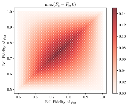
(a) Increase in Bell fidelity, see eq. (3), using $Z_{2B}$ distillation on Bell states undergoing bit flip errors (1).

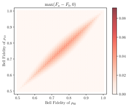
(b) Increase in Bell fidelity, see eq. (5), using $Z_{2B}$ distillation on Bell states undergoing depolarizing noise (4).

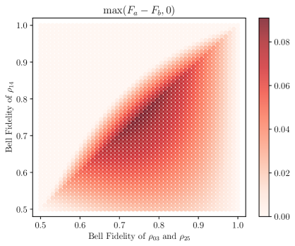
(c)

Figure 2: Algebraically obtained increase in Bell fidelity by different distillation protocols. The $x$ and $y$ axes represent the Bell fidelity of the states prior to distillation while the color corresponds to the increase (if any) in fidelity upon distillation.

III Circuit noise

Unlike the previous section in this section we relax the assumption that the circuit used for distillation is perfect and include gate noise and measurement error. The addition of these will greatly affect the ability to perform successful distillation. Motivated by the planar connectivity of superconducting qubits (and connecting to our experiments in the later sections), we consider circuits where Bell pairs need to be created locally and swapped so that the distillation circuit can be performed; see Fig. 3a as an example.

To model noise on measurements we apply a bit flip channel, ${\mathcal{D}}_{m}$, prior to measurement and noise on two-qubit gates is modelled by adding a two-qubit (global) depolarizing channel, ${\mathcal{N}}_{g}$, on the two qubits involved in the gate. Other sources of noise, such as imperfections in initializing the qubits to $\ket{0}$ and those in implementing single qubit gates, are ignored since these sources of noise can be comparatively smaller than measurement and two qubit gate noise. In the following, we will consider distillation as a function of these noise parameters versus the fidelity of the input Bell pairs.

III.1 Local Depolarizing noise

In the studies presented in this we section we vary the input Bell pair’s fidelity using local depolarizing channels similar to Sec. II.3. In Fig. 3 we show circuits for distilling Bell pairs under the noise model just described. Here, we add a qubit depolarizing channel in two places. These two places are before the first barrier (dotted vertical line) and between the second and third barriers in each of the sub-figures of Fig. 3. This allows us to independently control the asymmetry among the Bell pairs and fidelity of the Bell pairs prior to distillation.

III.1.1 Recurrence

(a)

(b)

Figure 3: Circuits for entanglement distillation with quantum channels $\Lambda_{p}$ and $\Lambda_{q}$ inserted at various stages.

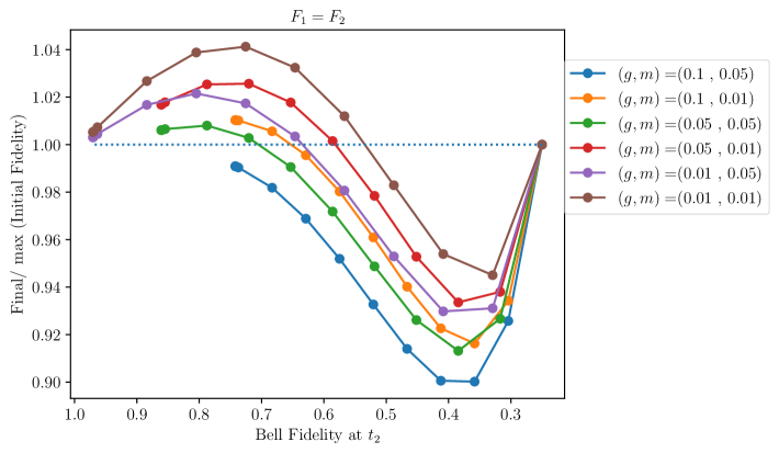
(a)

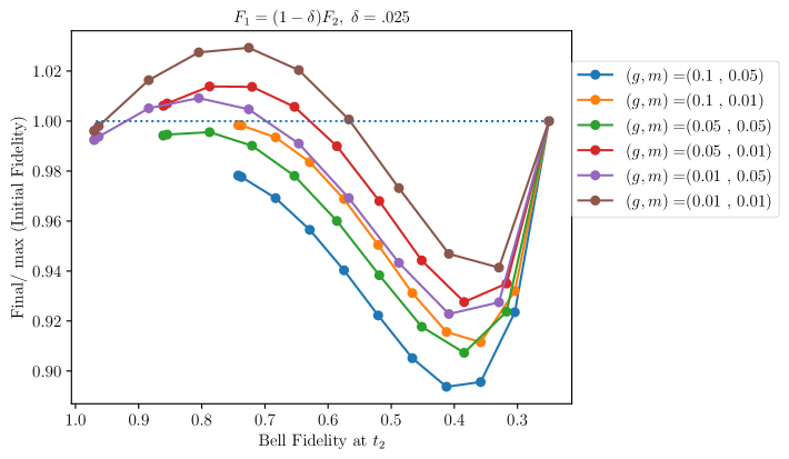
(b)

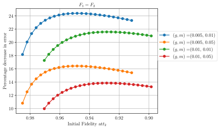
(c)

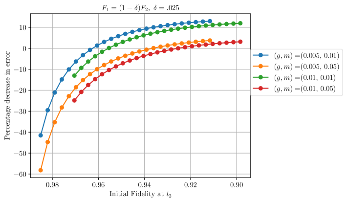
(d)

Figure 4: Results from simulation of recurrence with circuit noise described in Fig. 3a. Plots (4a) and (4b) show fractional change in Bell fidelity, $r$ (see eq. (15)), plotted against initial Bell fidelity $F_{b}$ (defined below (15)) for various gate and measurement errors, $g$ and $m$, respectively. The region where the plot remain above $r=1$ indicates where the noisy distillation circuit is beneficial. Plots (4c) and (4d) focus on high fidelity Bell pairs and shows the percentage decrease in Bell infidelity (defined in eq. (16)) plotted against initial fidelity $F_{b}$ for various gate and measurement errors.

We simulate the recurrence protocol ($Z_{2B}$) using the quantum circuit shown in Fig. 3a. In this circuit all four qubits are initialized to $\ket{0}$. First the circuit prepares two Bell states (across qubits $0-1$ and $2-3$) and then adds noise to the first Bell state (modelled via a depolarizing channel $\Lambda_{p}$ acting on the top qubit). This noise helps model asymmetry in the initial Bell pairs. In the next part after the first barrier (dotted line labelled $t_{0}$), the circuit swaps one half of each Bell pair creating a (physically) non-local Bell pair across qubits $0-2$ and $1-3$. Next, after the second barrier (dotted line labelled $t_{1}$), we apply a waiting error (modelled via a one-qubit depolarizing channel $\Lambda_{q}$ acting on qubits 1 and 2 that constitute one half of each Bell pair). The final part of the circuit, after the third barrier, carries out a distillation protocol described in Fig. 1a. All CNOT gates and measurements carry error, described by channels ${\mathcal{N}}_{g}$ and ${\mathcal{D}}_{m}$, respectively, as discussed in beginning of this section.

Variation in the performance of distillation with gate error, $g$, measurement error, $m$, and asymmetry between the initial Bell pairs is plotted in Fig. 4. In this figure, the ratio

$$r=F_{a}/F_{b}$$ (15)

is plotted against $F_{b}$, where $F_{a}$ is the Bell fidelity of the distilled Bell pair and $F_{b}$ is the maximum of the Bell fidelities among the non-local Bell pairs just prior to being distilled. The Bell fidelities $F_{1}$ and $F_{2}$ are of the Bell pairs just prior to the first barrier in Fig. 3a

In the first plot, Fig 4a, the two Bell pairs have equal Bell fidelity, i.e., $\Lambda_{p}$ in Fig. 3a is noiseless. For any fixed gate error, $g\in\{.01,.05,.1\}$, and measurement error, $m\in\{.01,.05\}$, we increase the parameter $q$ in the waiting error $\Lambda_{q}$ and plot $r$ (15) as a function of the initial Bell fidelity $F_{b}$. In each of these plots as the waiting error $q$ is increased from zero, the Bell fidelity prior to distillation, $F_{b}$, decreases while the ratio $r$ first increases, reaches a maximum, then decreases, reaches a minimum and finally tends to fixed value 1 at $F_{b}=.25$. Across different plots, if we fix the gate error $g$ but increase the measurement error $m$ we notice a decrease in $r$. On the other hand, if we fix the measurement error $m$, increasing the gate error $g$ has two effects. First, it decreases the initial Bell fidelity $F_{b}$ at $q=0$ (i.e., the plot begins at a smaller $F_{b}$ value) and also decreases the initial $r$ value corresponding to that initial Bell fidelity. Second, it shrinks the interval of $F_{b}$ values over which $r>1$.

In the second plot, Fig 4b, the two Bell pairs have unequal Bell fidelity, i.e., $\Lambda_{p}$ in Fig. 3a is noisy with $p\neq 0$. After the action of this noisy identity gate, the first Bell pair (across qubits $0$ and $1$) becomes more noisy than the second (across qubits $2$ and $3$) and Bell fidelity of the first Bell pair $F_{1}$ is $2.5\%$ lower than that of the second, $F_{2}$. Salient features of the plot in Fig. 4b resemble those of Fig. 4a discussed above. The key difference is that for fixed $g$ and $m$ values the value of $r$ in Fig. 4b are smaller than the corresponding values in Fig. 4a. In fact, we only see improvement in a small region where the gate and measurement errors are $\leq 1\%$.

In Fig. 4c and 4d we focus on smaller gate and measurement errors, $g=1\times 10^{-2}$ or $5\times 10^{-3}$ and $m=5\times 10^{-2}$ or $1\times 10^{-2}$. Here the $Y$ axis is the percentage decrease in error, i.e.,

$$\epsilon_{d}=\frac{F_{a}-F_{b}}{1-F_{b}}\times 100,$$ (16)

while the $X$ axis is the initial Bell fidelity $F_{b}$. We obtain points along these axis by varying the waiting error $q$ in $\Lambda_{q}$. Here, the initial Bell fidelity is typically greater than $0.9$ and we notice a $10\%-20\%$ decrease in error by performing distillation on Bell pairs with equal Bell fidelity (see Fig. 4c). When the Bell pairs have unequal Bell fidelity, recurrence does not necessarily decrease the error for very high Bell fidelity but manages to decreases error as the initial Bell fidelities become smaller (see Fig. 4d). This observation is consistent with results in Fig. 2a which show that the range of initial Bell fidelities where distillation improves is narrow when the initial Bell fidelities are high.

III.1.2 Three Bell Distillation

Next, we simulate the $ZX_{3B}$ protocol using the circuit in Fig. 3b. This circuit prepares three Bell pairs, which we label as $AA$, $BB$, and $CC$, initialized on qubits $0-1$, $2-3$, and $4-5$, respectively. Next, the circuit adds noise to Bell states $AA$ and $CC$ via $\Lambda_{p}$. After the first barrier (labelled $t_{0}$) a sequence of CNOT gates re-order the Bell pairs into $ABCABC$, such that one half of each Bell pair is separated from its other half by two qubits. After the second barrier, the circuit applies a waiting error (via channel $\Lambda_{q}$ acting on one half of each Bell pair), and finally, it carries out the $ZX_{3B}$ distillation protocol (see Sec. II.2).

(a)

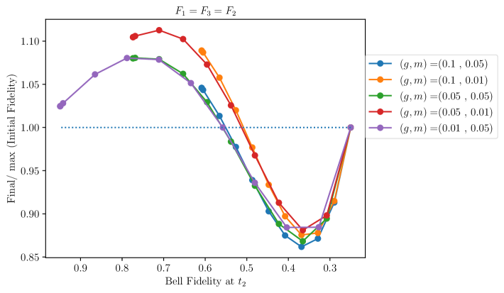
(b)

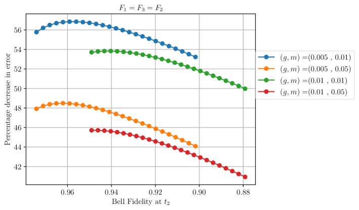
(c)

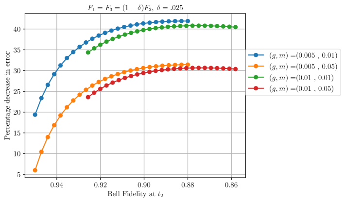
(d)

Figure 5: Results from simulation of $ZX_{3B}$ distillation with circuit noise given in Fig. 3b. Plots (5a) and (5b) show fractional change in Bell fidelity, $r$ plotted against initial Bell fidelity $F_{b}$ for various gate and measurement errors. The region of the plot above $r=1$ indicates where the noisy distillation circuit is beneficial. Plots (5c) and (5d) focus on low noise Bell pairs and show the percentage decrease in Bell infidelity plotted against initial fidelity $F_{b}$ for various gate and measurement errors.

The first plot in Fig. 5a describes the variation in the ratio $r$ as a function of the $F_{b}$ for fixed gate and measurement errors. All three Bell pairs have the same initial Bell fidelity. The variation in $r$ and $F_{b}$ with the gate error $g$ and measurement error $m$ are similar to those in Fig. 4a, described below eq. (15). For fixed $g$ and $m$, the ratio $r$ in Fig. 5a is typically higher than those in Fig. 4a when $r>1$. In addition, the value of $F_{b}$ at which $r$ shifts from a value greater than one to a value less than one is typically lower in Fig. 5a compared to Fig. 4a, i.e., the parameter region and amount by which distillation provides an improvement seem to be typically larger in Fig. 5a compared to Fig. 4a.

In Fig. 5b two of the Bell pairs, the first $AA$ pair across qubits $0-1$ and third $CC$ across qubits $4-5$, have lower Bell fidelity, than the second pair $BB$ across $2-3$, i.e. $F_{1}=F_{3}<F_{2}$. The noise parameter $p$ is such that the initial Bell fidelity $F_{1}=F_{3}=.975F_{2}$. As a result distillation protocol here can be seen as an attempt to improve the fidelity of one Bell pair using two Bell pairs with lower fidelity. Variation in improvement $r$ and $F_{b}$ with the gate error $g$ and measurement error $m$ is similar to those in Fig. 4b, described below eq. (15). For fixed $g$ and $m$, the ratio $r$ in Fig. 5a can be higher higher than those in Fig. 4b, however this need not be the case in general, even when $r>1$

The focus in Fig. 5c and 5d is on smaller gate and measurement errors, $g=1\times 10^{-2}$ or $5\times 10^{-3}$ and $m=5\times 10^{-2}$ or $1\times 10^{-2}$. As the error parameter $q$ is varied, we plot the percentage decrease in error against the initial Bell fidelity $F_{b}$. When the Bell pairs being distilled have equal fidelity initially we find a $40\%-50\%$ decrease in error, as shown in Fig. 5c. The decrease in error is lower when the when Bell pairs have unequal Bell fidelities initially, as shown in Fig. 5d; it is possible that error increases if the initial Bell fidelities are made even more unequal.

III.2 Global Depolarizing noise

In this section, we apply circuit noise to Bell pairs and degrade them under a global depolarizing noise channel ${\mathcal{N}}_{\lambda}$ (see Fig. 11 in App. G); this global noise is consistent with Clifford twirling [46, 47], which we will do experimentally in Sec. IV.1.

III.2.1 Two Bell Distillation

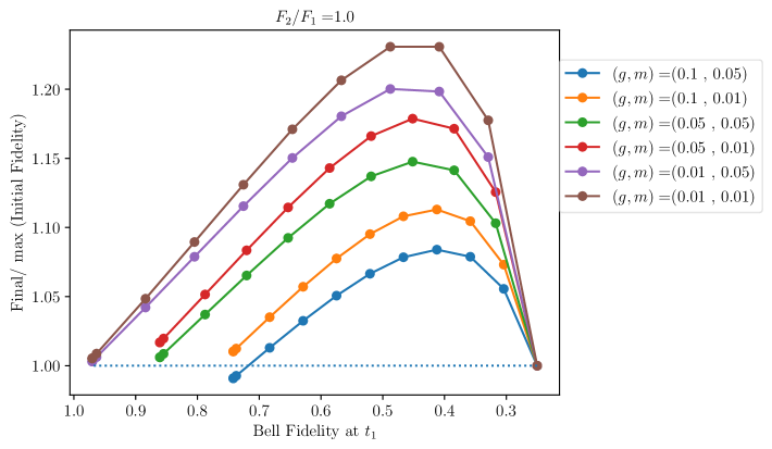
(a)

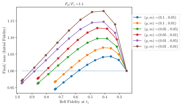
(b)

Figure 6: Results from simulation of recurrence $Z_{2B}$ with global depolarizing noise. Fractional change in Bell fidelity plotted against input Bell fidelity. Each curve has a different gate and measurement error. The two plots look at symmetric and asymmetry input Bell pairs.

We numerically study the performance of the recurrence distillation protocol ($Z_{2B}$) after the Bell pairs are degraded by a global depolarizing channel. The distillation circuit under study modifies the one in Fig. 3a by replacing local with global depolarizing noise during waiting (circuit available as Fig. 11a in App. G) In the first plot, see Fig. 6a, the Bell pairs are created with equal Bell fidelity, $F_{1}=F_{2}$. As the global depolarizing noise parameter $\lambda$ is increased, the fidelity of Bell pairs prior to distillation decreases. For any fixed gate and measurement error, as $\lambda$ is increased the ratio $r$, plotted on the y-axis, first increases reaches a maximum and then decreases to one. This ratio can be as high as 1.2, and it remains above one for a wider range of gate and measurement error values. This represents broad improvement from distillation. The improvements shrink as the gate and measurement error are increased. In Fig. 6b the Bell pairs have unequal Bell fidelity prior to distillation. This asymmetry is created by noise channel $\Lambda_{p}$ on qubit labelled 0 in Fig. 11a. A key qualitative effect of this asymmetry is in the ratio $r$. This ratio remains below one for higher initial Bell fidelities, thus shrinking the range of gate and measurement error values over which distillation presents an improvement. The improvement is also smaller in comparison to those reported in Fig. 6a.

III.2.2 Three Bell Distillation

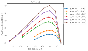
(a)

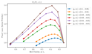
(b)

Figure 15: Results from simulation of $ZX_{3B}$ distillation with global depolarizing noise. Fractional change in Bell fidelity plotted against initial Bell fidelity. The curves are represent different gate and measurement errors. The two plots are symmetric and asymmetric initial Bell pair fidelities.

Here we continue from the previous section, but indicate results from the double selection ($ZX_{3B}$) protocol. The effect of global depolarizing noise on the $ZX_{3B}$ distillation protocol is similar to that of recurrence shown in Fig. 6 and described in Sec.III.2.1. However the value of $r$ is typically higher than those in the corresponding plots on Fig. 6 (see App. H for plots on Fig. 15).

IV Experimental Results and Device Noise

Given the simulations of the previous sections, we now want to consider distillation protocols on a real device. We run experiments on a 127 qubit device with fixed frequency qubits and fixed coupling, an IBM Eagle device ibm_kyiv. For the purposes of these experiments we consider smaller sections of the device with linear connectivity and run each experiment in parallel across different sections of the device in order to obtain more statistics on noise. For more device details see Appendix E.

For each circuit we estimate the fidelity of the Bell state using direct fidelity estimation by measuring three circuits (see App. B for more). However, this scheme does have measurement error. In contrast to [42], here we choose to not correct for measurement errors due to issues that can cause potentially non-physical and or unexpectedly high fidelities (see, e.g., discussion in Ref. [48]). Our experimental results thus provide a good lower bound on the Bell fidelities.

IV.1 Two Bell distillation experiment with global depolarizing noise

Following from the discussion on Sec. III.2, first, we experimentally study the recurrence protocol under global depolarizing noise. This global depolarizing channel ${\mathcal{N}}_{\lambda}$ is implemented using layers of two-qubit Clifford circuits. The first half of such a circuit is composed of multiple applications of a length-$k$ random sequence of two-qubit Clifford gates and the second half is the inverse of the first half. This inverse is simply the mirror image of the first half and these layers are called mirror Clifford layers [49] (see Fig. 12 in App. G for an example of such a circuit with two layers in the first half).

These measurements are carried out on a set of four adjacent qubits on a device. On 13 such sets we carry out the experiment outlined above for different fixed $k\in\{0,2,4,6,8,10,12\}$. For each $k$ we obtain an average of 13 sets of the before and after distillation Bell fidelities along with the acceptance probability for distillation. These are plotted in Fig. 7. In Fig. 7a we plot the acceptance ratio as a function of the initial Bell fidelity. The dots represent points from the experiment while the straight line is obtained from numerics. In Fig. 7b we plot the ratio $r$ as a function of the initial Bell fidelity prior to global depolarizing noise. The blue dots represent data while the orange curve represents the theoretically expected curve. This theoretical curve from eq. (13) assumes noiseless gates and measurement. There is fairly good agreement between the theory curves and the experiment data, particularly considering the x-axis is subject to systematic error due to measurement error and the theory calculation assumes the distillation circuit is perfect. This demonstrates that under some conditions on the device we can see an improvement due to distillation, however the improvement arises from a systematic procedure to degrade the Bell pairs via global depolarizing noise. Furthermore, high fidelity Bell pairs do not improve in this experiment.

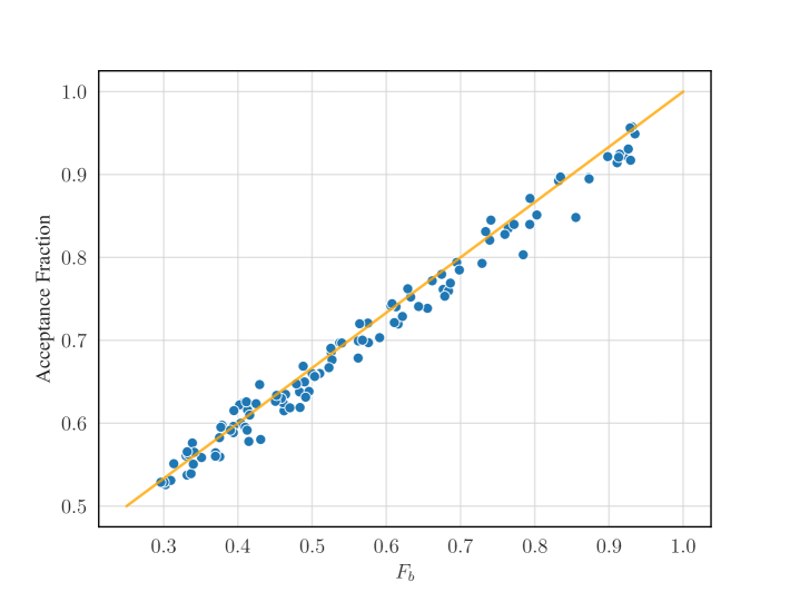
(a)

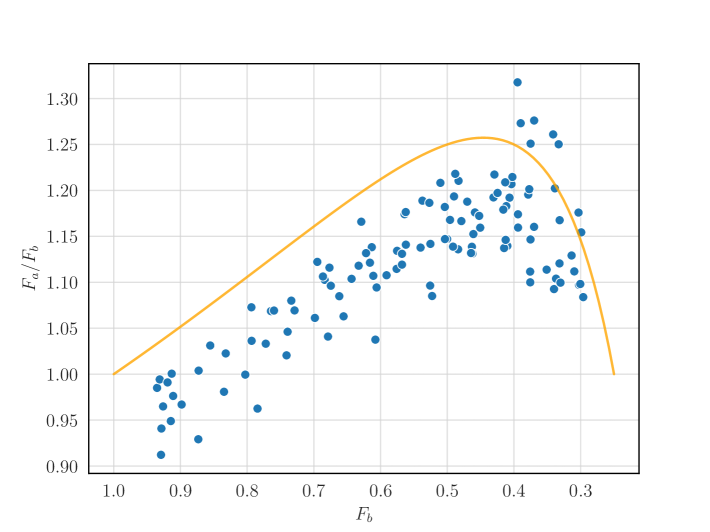
(b)

Figure 7: Experimental results (blue) on ibm_kyiv for the $Z_{2B}$ recurrence distillation protocol with global depolarizing noise. Orange curves are theory assuming perfect distillation.

IV.2 Two Bell distillation experiment with idle noise

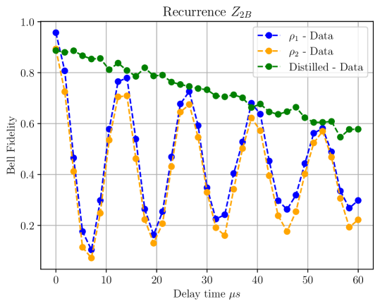
Figure 8: Experimental data from qubits (0,1,2,3) of ibm_kyiv (points) showing increase in the Bell fidelity under $Z_{2B}$ distillation of qubits undergoing coherent $ZZ$ errors.

Here we consider a more natural experiment, create a Bell pair and wait a time $t$ for the Bell fidelity to decay under device $T_{1}/T_{2}$ noise and then measure (note we apply a standard echo sequence to remove low frequency noise). These $T_{1}/T_{2}$ noise channels are not simply Pauli channels and they are not an effective error obtained from averaging over random iterations, as we did in the previous section. However, an effective $T_{1}/T_{2}$ idling error is not obtained by simply waiting on an actual device; due to $ZZ$ interactions between neighboring pairs the Bell state fidelity can strongly degrade. We show a simple example of this in Fig.(8). Here we can get tremendous improvement in the Bell fidelity, but this is because we allowed the Bell fidelity to decrease via a coherent error term; the purity of the state is unchanged. One has to be careful of similar situations where distillation provides an apparent benefit, but where improvement could more easily be achieved without post-selection. In this example, the $ZZ$ coherent error term can be also be canceled by applying staggered dynamical decoupling (DD) [50, 51, 52] (see App. G, Fig. 13a). With staggered DD, the circuit is now well described by $T_{1}$ and $T_{2}$ errors.

Once we apply staggered DD, typical data is shown in Fig. 9 with dotted lines. We see some natural features of the experiments. One, the starting Bell fidelity is lower than one due to the creation and swap operations (for instance see the Bell fidelity in Figs. 9a and 9b at $t=0$ is less than one). Second, there is a natural asymmetry in the initial fidelity due to the variability of noise parameters between qubits (for instance the Bell fidelity of the two bell pairs in Fig. 9b are unequal). Third, depending on the distillation protocol used, $Z_{2B}$ or $X_{2B}$, one may or may not see broad improvement in Bell fidelity (see Fig. 9d with improvement and 9c without); however we do not yet see broad across the device. To understand these features better we look to build a more involved device noise model.

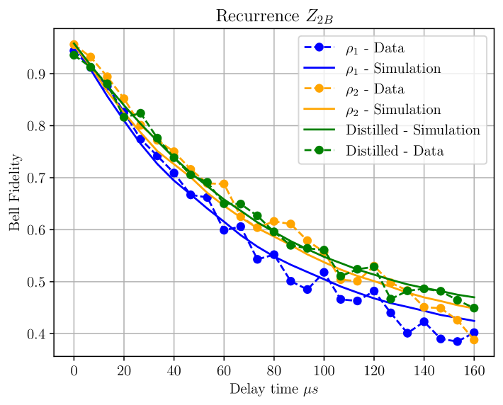
(a) Bell fidelity of the non-local Bell pairs prior to and after recurrence $Z_{2B}$.

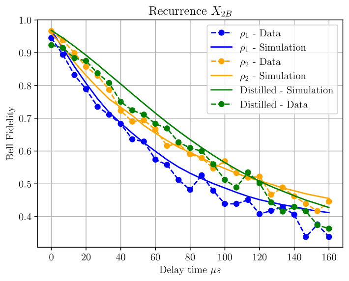
(b)

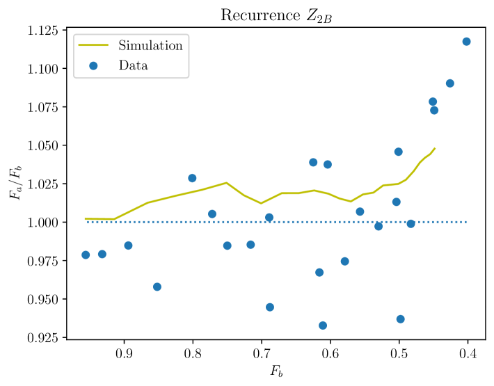
(c)

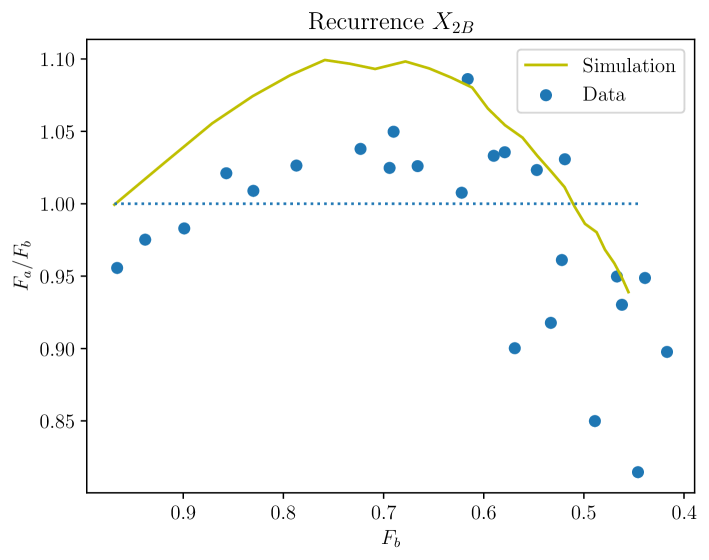
(d)

Figure 9: Data and simulation for recurrence $Z_{2B}$ and $X_{2B}$ on qubits (0,1,2,3) of ibm_kyiv. Solid lines are simulations assuming reported noise parameters as described in Table. 3 and 4 of App. E. Additional plots in App. H, Fig. 16 and 17

IV.3 Device Model and Numerics

To build a more involved device model we must include $T_{1}/T_{2}$ noise [44, 45] (see App. F for a mathematical description) during the wait periods. These include when the swap is occurring, when the Bell states are idle and when the measurements are occurring. Furthermore, due to the effect described in Ref. [53] it’s not enough to use the bare $T_{1}/T_{2}$ even though we performed staggered echo sequences. We must still include the $ZZ$ terms and simulate the echo sequence to get the proper decay of the Bell states during the wait. We continue to add in the gate and measurement noise as described in Sec. III.1. We pull the $ZZ$, $T_{1}$, $T_{2}$, gate times and measurement error from the backend of the device (see Tables 3 and 4 in App. E).

For recurrence $Z_{2B}$ the simulations are given by the solid lines in Fig. 9a and we notice fairly good agreement between the experimental and numerical simulations. Confirming the general trend of the data is consistent with the calibration data. However, the figure does not indicate consistent improvement in Bell fidelity with distillation. To get improvements we notice (see Table 3 in App. E) that, in general, the dominant source of noise on the qubits under consideration is $T_{2}$ noise (i.e., $Z$ errors) while the $Z_{B2}$ catches $T_{1}$ noise, i.e., $X$ and amplitude damping type errors.

The $X_{2B}$ distillation protocol catches $Z$ errors. Results from implementing this protocol in both simulation and experiment is given in Fig. 9b. In this figure, there is reasonable agreement between the experimental data and numerical simulations. In addition, notice there is general improvement in Bell fidelity, indicating that the likely dominant source of $T_{2}$ errors are caught by $X_{2B}$ recurrence. Improvements are not seen for higher Bell fidelities. This likely occurs due to both measurement errors and asymmetry in Bell fidelities of the two Bell pairs being distilled. The former are not removed by distillation while the latter generally shrink the noise region where distillation shows improvement. In specific cases simulations indicate that lowering measurement errors to zero can allow distillation to give improvements even for high fidelity Bell pairs.

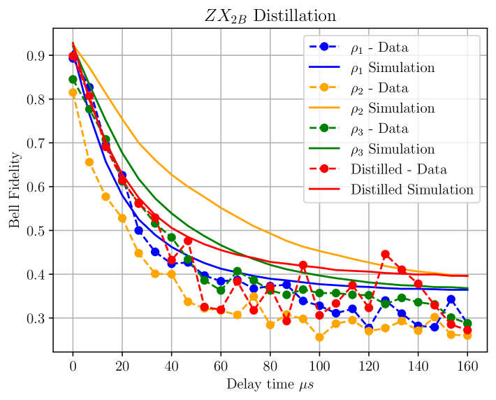
(a)

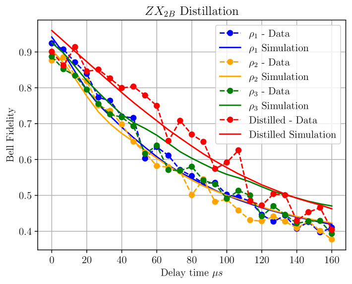
(b) Bell fidelity of the non-local Bell pairs prior to and after distillation on qubits (3,4,5,6,7,8). Simulations fits the data well.

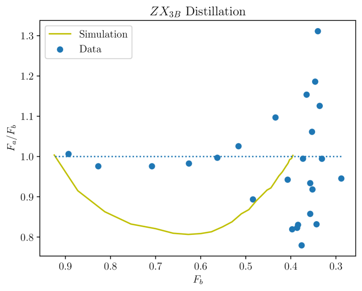
(c)

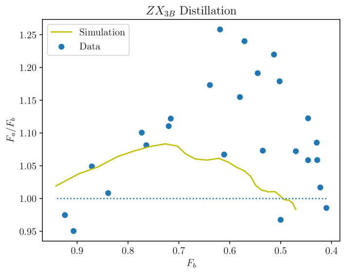
(d)

Figure 10: Data and simulation for $ZX_{3B}$ recurrence on ibm_kyiv. Solid lines are simulations assuming reported noise parameters as described in Table. 5 and 6 of App. E. Additional plots in App. H, Fig. 19 and Fig. 18

IV.4 Three Bell distillation experiment with idle noise

Using the same technique for experiment and numbers as in the previous sections we extend the experiment to the three Bell ($ZX_{3B}$) protocol (circuit available in App. G, Fig. 14) and results of this are shown in Figs. 10. Again, we get reasonable agreement with the numerics using just the backend calibration parameters. We see two cases, in the first (see Fig. 10a) we have small acceptance ratio and no real improvement in the Bell state; here the noise parameters are quite large. In the second set of data (see Fig. 10d) we see some strong improvement from distillation, but this does not persist well to the highest fidelities and therefore limits us from distributing higher fidelity entanglement this way. In places where we find improvement (say at e.g. $50\mu$ s in Fig. 10b) one can experience a loss of data, i.e, an acceptance probability below $50\%$.

V Conclusions

We carried out both a numerical and experimental analysis of some basic distillation protocols. The simplest numerical analysis in Sec. II adds asymmetry among the Bell pairs since the asymmetry can be inherent in the way multiple Bell pairs are arranged prior to distillation. That analysis points at regions in the noise parameter space where entanglement distillations can provide improvements. A more involved analysis using device characterization data, non-Pauli noise channels, and modelling the echo sequence in our experiment allows us to obtain reasonable agreement with the experimental data obtained from entanglement distillation. The noise models indicate how practical difficulties in distillation come from (1) a natural asymmetry among the Bell pairs being distilled; (2) understanding the noise which distillation must remove; (3) measurement noise; and (4) fixing a metric of success for distillation. When the metric of success is improving average Bell fidelity over several pairs or removing coherent errors in a single pair, we find the simplest distillation protocols can provide broad improvements (see discussions in Sec. IV.1 and Sec. IV.2). However, for using distilled Bell pairs in modular computing it is valuable to consider a stricter metric: distill (physically) non-local Bell pair with higher fidelity than what can be obtained using other available means. This work leaves open the question of broadly improving upon this metric. One way to obtain such improvements using the protocols discussed here would be to make noise more uniform on the Bell pairs; another would be to lower the measurement errors on the qubits; while a third would be to go beyond the types of protocols discussed in this work.

In our analysis, we found it particularly useful to view distillation as stabilizer checks. This made it ‘easy’ to view different distillation protocols as tools to catch different types of errors (which need not be Pauli errors, and are not necessarily modeled as such here either). This can help guide the selection of distillation protocols depending on the source of the dominant noise in one’s error model.

A variety of prior work focusses on the optimal trade-offs between success probability and Bell fidelity upon distillation over Pauli noise channels. For practical studies, our work motivates the study of $T_{1}/T_{2}$ noise channels (these have experimentally available noise parameters) and benchmarking protocols when starting with unequal bell pairs that incur measurement errors.

VI Acknowledgments

We thank Sam Stein, Michael DeMarco, Andrew Cross and John Smolin for helpful discussions. This work was supported by the U.S. Department of Energy, Office of Science, National Quantum Information Science Research Centers, Co-design Center for Quantum Advantage (C2QA) under contract number DE-SC0012704.

Appendix A Notation

Let $\{\ket{0},\ket{1}\}$ denote the standard basis of a qubit Hilbert space ${\mathcal{H}}$ (sometimes called the $Z$ basis), $\ket{\pm}:=(\ket{0}\pm\ket{1})/\sqrt{2}$ denote the so-called Hadamard basis, and $H:=|+\rangle\langle 0|+|-\rangle\langle 1|$ represent the Hadamard gate. Let $X=|0\rangle\langle 1|+|0\rangle\langle 1|$, $Y=i|0\rangle\langle 1|-i|0\rangle\langle 1|$, and $Z=|0\rangle\langle 0|-|1\rangle\langle 1|$, together with the $2\times 2$ identity, $\mathbb{I}$, denote the Pauli matrices ${\mathcal{P}}$. Any two square matrices $P,Q$ are said to commute when $PQ=QP$ and anti-commute when $PQ=-QP$. Note any two Pauli matrices either commute or anti-commute.

The qubit X-dephasing (bit flip) channel,

$${\mathcal{D}}_{q}(\rho)=(1-q)\rho+qX\rho X,$$ (17)

applies the Pauli $X$ operator with probability $0\leq q\leq 1/2$. The qubit depolarizing channel,

$$\begin{aligned} \Lambda_{p}(\rho)&=(1-p)\rho+\frac{p}{3}(X\rho X+Y\rho Y+Z\rho Z),\\ &=(1-\frac{4}{3}p)\rho+\frac{4p}{3}{\rm Tr}(\rho)\frac{\mathbb{I}}{2},\end{aligned}$$ (18)

applies Pauli $X,Y,$ and $Z$ operators with equal probability $p/3$ and the identity operator $\mathbb{I}$ with probability $1-p$ where $0\leq p\leq 1$. We use ${\mathcal{I}}$ to denote the identity channel, ${\mathcal{I}}(\rho)=\rho$ for all operators $\rho$.

The fidelity of a two-qubit density operator $\rho$ with the maximally entangled state,

$$\ket{\phi}=(\ket{00}+\ket{11})/\sqrt{2},$$ (19)

is what we call the Bell fidelity, $F:=\langle\phi|\rho|\phi\rangle$. The Bell fidelity can be estimated directly from Pauli measurements (see App. B). We refer to $1-F$ as the infidelity with the Bell state (19). The two-qubit CNOT gate with $0^{\text{th}}$ qubit as control and first qubit as target is $CNOT_{01}=|0\rangle\langle 0|\otimes\mathbb{I}+|1\rangle\langle 1|\otimes X$.

The tensor product of Pauli matrices ${\mathcal{P}}$ on $n$-qubits is sometimes called a Pauli string. We use a compressed notation to represent such a string by suppressing the identity matrix and using subscript to denote the system label. For instance with $n=3$ we denote $Z\otimes\mathbb{I}\otimes X$ by $Z_{0}X_{2}$.

Appendix B Direct Bell fidelity estimation

A two-qubit state, $\rho$, has Bell fidelity,

$$F=\langle\phi|\rho|\phi\rangle=\frac{1}{4}(1+\langle ZZ\rangle_{\rho}+\langle XX\rangle_{\rho}-\langle YY\rangle_{\rho})$$ (20)

where $\langle N\rangle_{\rho}:={\rm Tr}(N\rho)$. The Bell fidelity can be computed by measuring expectation value of $ZZ,XX,$ and $YY$ operators. To compute $\langle ZZ\rangle_{\rho}$ one may measure each qubit of $\rho$ in the $Z$ basis, obtain probabilities $p_{ij}$ for measurement outcome corresponding to basis $\ket{ij}$ and then evaluate $\langle ZZ\rangle_{\rho}=2(p_{00}+p_{11})-1$.

Expectation values for $XX$ and $YY$ can be computed in an analogous manner by measuring qubits in the $X$ and $Y$ basis instead of $Z$. Thus, to measure the Bell fidelity this way one does three different measurement experiments, one for each Pauli measurement basis. Given a circuit for measuring a qubit in the $Z$ basis one can measure in the $X$ and $Y$ basis by applying $H$ and $H\cdot S^{{\dagger}}$, respectively, prior to measuring in the $Z$ basis, where $S=\text{diag}(1,-i)$ is $\sqrt{Z}$.

Appendix C A general protocol for distillation

Both recurrence and the $ZX_{3B}$ protocols in Sec. II of the main text can be viewed as special cases of those in [54, 55]. These distillation protocols can be viewed in a unified way using a slightly different notation as follows.

Let ${\mathcal{H}}_{Ai}$ and ${\mathcal{H}}_{Bi}$ each be a qubit Hilbert space, ${\mathcal{H}}_{i}:={\mathcal{H}}_{Ai}\otimes{\mathcal{H}}_{Bi}$ be a two-qubit Hilbert space, ${\mathcal{H}}_{A}:=\otimes_{i=1}^{n}{\mathcal{H}}_{Ai}$ and ${\mathcal{H}}_{B}:=\otimes_{i=1}^{n}{\mathcal{H}}_{Bi}$ each be $n$-qubit Hilbert spaces, and $\rho_{AB}$ be a $2n$-qubit state. To distill a single two-qubit state from $\rho_{AB}$ one applies some unitary $U=U_{A}\otimes U_{B}$ to $\rho_{AB}$ then post-selects for agreement on $Z$ measurements made on $2(n-1)$ qubits. Let the unmeasured system be labeled $0$. To describe the post-selected state consider $T=\mathbb{I}_{0}\otimes L$ where $\mathbb{I}_{0}$ is the identity on ${\mathcal{H}}_{0}$, $L=\otimes_{i=1}^{n-1}P_{i}$, and $P_{i}=|00\rangle\langle 00|+|11\rangle\langle 11|$ is a projector defined on ${\mathcal{H}}_{i}$. The post-selection succeeds with probability

$$p_{a}={\rm Tr}(TU\rho U^{{\dagger}}T^{{\dagger}})$$ (21)

and results in a state

$$\rho^{\prime}=\frac{1}{p_{a}}{\rm Tr}_{i\neq 0}(TU\rho U^{{\dagger}}T^{{\dagger}}),$$ (22)

where the partial trace is over all spaces ${\mathcal{H}}_{i}$ except $i=0$. The fidelity of the post-selected state is

$$F={\rm Tr}(\rho^{\prime}\phi).$$ (23)

Appendix D Distilled fidelity calculation

As explained at the end of Sec. II, the recurrence protocol post-selects away errors on qubits $2$ and $3$ that anti-commute with $Z_{2}Z_{3}$. This idea can be used to compute the final fidelity $F_{a}$ in (5) and acceptance probability $p_{s}$ in (6). In Fig. 1a, suppose

$$\rho_{02}={\mathcal{I}}\otimes{\mathcal{P}}_{\textbf{p}}(\rho)\quad\text{and}\quad\rho_{13}={\mathcal{I}}\otimes{\mathcal{P}}_{\textbf{q}}(\rho),$$ (24)

where ${\mathcal{P}}_{\textbf{p}}(\rho):=p_{I}\rho+p_{x}X\rho X+p_{y}Y\rho Y+p_{z}Z\rho Z$ is a qubit Pauli channel, each $p_{i}\geq 0$, and $\sum_{i\in\{I,x,y,z\}}p_{i}=1$. The collection of the Pauli errors not caught by recurrence are detailed in Table 1. In this table, the first column denotes errors on qubits $2$ and $3$ that commute with $Z_{2}Z_{3}$, and are thus not post-selected away by recurrence, the second column denotes the probability of these errors, and the third column denotes the effective error after post-selection on qubit labelled $2$. Setting $p_{x}=p_{y}=p_{z}=p/3$ and $q_{x}=q_{y}=q_{z}=q/3$ and summing the entries in the second column gives the acceptance probability $p_{s}$ (6) while summing those entries in the second column where the effective error is $I_{2}$ and normalizing by $p_{s}$ gives the Bell fidelity of the distilled state $F_{a}$ (5).

Error	Probability	Transformed Error
$\mathbb{I}$	$p_{I}q_{I}$	$\mathbb{I}_{2}$
$Z_{3}$	$p_{I}q_{z}$	$Z_{2}$
$X_{2}X_{3}$	$p_{x}q_{z}$	$X_{2}$
$X_{2}Y_{3}$	$p_{x}q_{y}$	$Y_{2}$
$Y_{2}X_{3}$	$p_{y}q_{x}$	$Y_{2}$
$Y_{2}Y_{3}$	$p_{y}q_{y}$	$X_{2}$
$Z_{2}$	$p_{z}q_{I}$	$Z_{2}$
$Z_{2}Z_{3}$	$p_{z}q_{z}$	$\mathbb{I}_{2}$

Table 1: Accepted errors by recurrence and their effect: Pauli error not post-selected away by recurrence (see Sec. II.1), their probability, and their effect on the final distilled Bell pair.

For the $ZX_{3B}$ distillation protocol, we may derive the acceptance probability $p_{s}$ in (9) and Bell fidelity upon acceptance $F_{b}$ in (8) using a procedure analogous to the one above. Suppose in Fig. 2c

$$\begin{aligned} \rho_{03}&={\mathcal{I}}\otimes{\mathcal{P}}_{\textbf{p}}(\rho),\\ \rho_{14}&={\mathcal{I}}\otimes{\mathcal{P}}_{\textbf{q}}(\rho),\quad\text{and}\\ \rho_{25}&={\mathcal{I}}\otimes{\mathcal{P}}_{\textbf{r}}(\rho).\end{aligned}$$ (25)

then we list the collection of errors not caught by the $ZX_{3B}$ distillation protocol in Table 2. In this table, the first, second and third column represent the accepted errors (those which commute with both $Z_{3}Z_{4}Z_{5}$ and $X_{4}X_{5}$), their probability and their effect on qubit $3$ after qubits $4$ and $5$ are measured, respectively. Setting $p_{x}=p_{y}=p_{z}=r_{x}=r_{y}=r_{z}=p/3$, and $q_{x}=q_{y}=q_{z}=q/3$ and summing the entries in the second column gives the acceptance probability, $p_{s}$ in (9), while summing the entries in the second column corresponding to no error ($\mathbb{I}$) in the third and normalizing by $p_{s}$ gives the fidelity after distillation, $F_{a}$ in (8).

Error	Probability	Transformed Error
$\mathbb{I}$	$p_{I}q_{I}r_{I}$	$\mathbb{I}_{3}$
$X_{4}X_{5}$	$p_{I}q_{x}r_{x}$	$\mathbb{I}_{3}$
$Z_{4}Z_{5}$	$p_{I}q_{z}r_{z}$	$Z_{3}$
$Y_{4}Y_{5}$	$p_{I}q_{y}r_{y}$	$Z_{3}$
$X_{3}X_{5}$	$p_{x}q_{I}r_{x}$	$X_{3}$
$X_{3}X_{4}$	$p_{x}q_{x}r_{I}$	$X_{3}$
$X_{3}Z_{4}Y_{5}$	$p_{x}q_{z}r_{y}$	$Y_{3}$
$X_{3}Y_{4}Z_{5}$	$p_{x}q_{y}r_{z}$	$Y_{3}$
$Z_{3}$	$p_{z}q_{I}r_{I}$	$Z_{3}$
$Z_{3}X_{4}X_{5}$	$p_{z}q_{x}r_{x}$	$Z_{3}$
$Z_{3}Z_{4}Z_{5}$	$p_{z}q_{z}r_{z}$	$\mathbb{I}_{3}$
$Z_{3}Y_{4}Y_{5}$	$p_{z}q_{y}r_{y}$	$\mathbb{I}_{3}$
$Y_{3}X_{5}$	$p_{y}q_{I}r_{x}$	$Y_{3}$
$Y_{3}X_{4}$	$p_{y}q_{x}r_{I}$	$Y_{3}$
$Y_{3}Z_{4}Y_{5}$	$p_{y}q_{z}r_{y}$	$X_{3}$
$Y_{3}Y_{4}Z_{5}$	$p_{y}q_{y}r_{z}$	$X_{3}$

Table 2: Accepted errors by $ZX_{3B}$ and their effect: Pauli error not post-selected away by the $ZX_{3B}$ protocol (see Sec. II.2), their probability, and their effect on the final distilled Bell pair.

Appendix E Device Overview

Experiments were carried out on IBM’s fixed-frequency transmon superconducting processor, ibm_kyiv. This is a 127 qubit chip with qubits arranged in a heavy-hexagonal lattice which reduces cross-talk with reasonable overhead in circuit layout mapping. This processor is from IBM’s Eagle processor family which use the echoed cross-resonance gate for its entangling gate and features multiplexed readout. To support the higher qubit count, the chip features multi-layer wiring with care taken to reduce the effects of quantum and classical cross-talk. This architecture results in a median $T_{1}$ and $T_{2}$ of 276 and 122 respectively and median ECR gate error and readout error of $1.1\text{\times}{10}^{-2}$ and $6.0\text{\times}{10}^{-3}$ respectively. Tables 3,  4,  5, and 6 give error parameters for specific qubits on which distillation experiments and simulation were discussed in the main text.

Qubit	$T_{1}~(\mu s)$	$T_{2}~(\mu s)$	Measurement Error
0	257.944	323.573	6.5 $\times 10^{-3}$
1	477.815	224.595	9.1 $\times 10^{-3}$
2	263.123	123.047	4.3 $\times 10^{-3}$
3	260.839	232.639	4.6 $\times 10^{-3}$

Qubit 1	Qubit 2	$ZZ$ Rate (Hz)	ECR Error
0	1	-52860.4	7.75153 $\times 10^{-3}$
1	2	-55319.3	10.3203 $\times 10^{-3}$
2	3	-45908	4.2953 $\times 10^{-3}$

Table 3: Single qubit and two-qubit error rates from ibm_kyiv last updated on 2024-05-14 at 07:45:06 UTC used for simulation of recurrence $Z_{2B}$. Measurement delay is $1.24\mu s$. The CNOT error rate is taken to be the ECR error rate and kept the same when role of target and control qubits is reversed.

Qubit	$T_{1}~(\mu s)$	$T_{2}~(\mu s)$	Measurement Error
0	276.892	312.245	2.5 $\times 10^{-3}$
1	512.747	218.116	2.6 $\times 10^{-3}$
2	236.636	98.102	4.2 $\times 10^{-3}$
3	330.719	232.639	11.2 $\times 10^{-3}$

Qubit 1	Qubit 2	$ZZ$ Rate (Hz)	ECR Error
0	1	-52860.4	4.43472 $\times 10^{-3}$
1	2	-55319.3	8.10392 $\times 10^{-3}$
2	3	-45908	4.03714 $\times 10^{-3}$

Table 4: Single qubit and two-qubit error rates from ibm_kyiv last updated on 2024-05-15 at 16:05:02 UTC used for simulation of recurrence $X_{2B}$. Measurement delay is $1.24\mu s$. The CNOT error rate is taken to be the ECR error rate and kept the same when role of target and control qubits is reversed.

Qubit	$T_{1}~(\mu s)$	$T_{2}~(\mu s)$	Measurement Error
3	410.738	232.639	4.2 $\times 10^{-3}$
4	429.253	152.675	16.9 $\times 10^{-3}$
5	365.064	384.404	6.8 $\times 10^{-3}$
6	294.473	146.729	1.6 $\times 10^{-3}$
7	339.754	371.239	3.4 $\times 10^{-3}$
8	458.343	259.075	2.7 $\times 10^{-3}$
59	269.232	78.7512	2.4 $\times 10^{-3}$
60	273.893	285.543	6 $\times 10^{-3}$
61	318.205	152.633	7.9 $\times 10^{-3}$
62	255.428	25.5405	23.6 $\times 10^{-3}$
63	275.333	115.334	7.3 $\times 10^{-3}$
64	231.769	47.6543	3.8 $\times 10^{-3}$

Table 5: Single qubit error rates from ibm_kyiv last updated on 2024-05-17 at 05:54:35 UTC used for simulation of the three bell experiment. Measurement delay is $1.24\mu s$

Qubit 1	Qubit 2	$ZZ$ Rate (Hz)	CNOT Error
3	4	-48982	8.49846 $\times 10^{-3}$
4	5	-39813.1	11.4476 $\times 10^{-3}$
5	6	-76347.7	8.78052 $\times 10^{-3}$
6	7	-57303.5	16.352 $\times 10^{-3}$
7	8	-40264.1	8.80976 $\times 10^{-3}$
59	60	-127831	13.0765 $\times 10^{-3}$
60	61	-38618.7	7.85857 $\times 10^{-3}$
61	62	-57210.3	13.1797 $\times 10^{-3}$
62	63	-55771.1	13.9869 $\times 10^{-3}$
63	64	-40636.1	6.07738 $\times 10^{-3}$

Table 6: Two qubit error rate and $ZZ$ rate from ibm_kyiv last updated on 2024-05-17 at 05:54:35 UTC used for simulation of the three bell distillation protocol. The CNOT error rate is taken to be the same when role of target and control qubits is reversed.

Appendix F $T_{1}$/$T_{2}$ Channel

Noise on a superconducting qubit can be described using a damping-dephasing channel [44] that may be expressed as [45],

$${\mathcal{M}}(\rho)=\sum_{i}O_{i}\rho O_{i}^{{\dagger}},$$ (26)

where $O_{0}=\sqrt{1-p}(|0\rangle\langle 0|+\sqrt{1-g}|1\rangle\langle 1|)$, $O_{1}=\sqrt{g}\ket{0}\bra{1}$, $O_{2}=\sqrt{p}(|0\rangle\langle 0|-\sqrt{1-g}|1\rangle\langle 1|)$, $0\leq p\leq 1/2$ represents dephasing and $0\leq g\leq 1$ represents damping probability. The channel maps an input density operator with Bloch vector $\textbf{r}=(x,y,z)$ to an output with Bloch coordinates $\big{(}(1-2p)\sqrt{1-g}x,(1-2p)\sqrt{1-g}y,(1-g)z+g\big{)}$. When the output coordinates are parametrized as $(e^{-t/T_{2}}x,e^{-t/T_{2}}y,e^{-t/T_{1}}z+1-e^{-t/T_{1}})$ then

$$g=1-e^{-t/T_{1}},\quad p=(1-e^{-t(1/T_{2}-1/2T_{1})})/2,$$ (27)

and $2T_{1}\geq T_{2}$ When $p=0$ or $T_{2}=2T_{1}$, ${\mathcal{M}}$ is an amplitude damping channel mapping $\ket{1}$ to $\ket{0}$ with probability $g$. When $g=0$, or $T_{1}=\infty$, ${\mathcal{M}}$ is a pure dephasing channel that applies a $Z$ error with probability $p$. If a qubit with fixed $T_{1}$ and $T_{2}$ parameters waits idle for a time $t$ then channel modelling noise on this qubit, ${\mathcal{M}}_{t}$, is the ${\mathcal{M}}$ channel with paramters $g$ and $p$ depend on $t,T_{1},$ and $T_{2}$, as indicated in (27).

Appendix G Circuits for noise and distillation

Here we present the circuits used in the distillation protocols of the main text, as well as the modifications to those circuits that enabled us to study them under various types of noise.

(a)

(b)

Figure 11: Circuits for simulation of entanglement distillation with global depolarizing channel ${\mathcal{N}}_{\lambda}$ replacing the local depolarizing noise between $t_{1}$ and $t_{2}$ barriers in Fig. 3 of the main text.

Figure 12: Circuit for implementing recurrence under global depolarizing noise using mirror Clifford layers

(a)

(b)

Figure 13: Circuit(s) for the $Z_{2B}$ recurrence protocol with idling noise. In both circuits, two Bell pairs are created prior to time label $t_{0}$, between $t_{0}$ and $t_{1}$ the first and second qubits are swapped and a delay is added from $t_{1}$ to $t_{2}$. The delay inteval $t_{2}-t_{1}$ is parametrized as $n\delta t$ where $\delta t$ is variable and fixed integer $n$ is the number of times the $ZZ$ sequence $W_{\delta t,k}$ is applied. Control phase angles in each sequence are $\theta_{jk}=f_{k}2\pi\omega_{j}\delta t/n$ where $1\leq k\leq n$, $0\leq j\leq 2$, $f_{k}=1$ if $k<n/2$ and $-1$ otherwise, $\omega_{j}$ is the $ZZ$ frequence between qubits $j$ and $j+1$. In Fig. 13a after time $t_{2}$ Pauli basis measurements are carried out on each qubit to determine the Bell fidelity (see App. B for details). In Fig. 13b after $t_{2}$, $ZZ$ measurements are carried out on qubits $1$ and $3$ while qubits $0$ and $2$ are measured in the Pauli basis for Bell fidelity estimation.

(a)

(b)

Figure 14: Circuit(s) for $ZX_{3B}$ distillation with idling noise. In both circuits, three Bell pairs are created prior to time label $t_{0}$, between $t_{0}$ and $t_{1}$ the Bell pairs are swapped (see Sec. III.1.2 for details) and a delay is added from $t_{1}$ to $t_{2}$ (in a mannar analogous to that in Fig. 13). In Fig. 14a after time $t_{2}$ Pauli basis measurements are carried out on each qubit to determine the Bell fidelity (see App. B for details). In Fig. 14b after $t_{2}$, $ZZZ$ amd $IXX$ measurements are carried out (as explained in Sec. II.2) while qubits $0$ and $3$ are measured in the Pauli basis for Bell fidelity estimation.

Appendix H Additional plots from simulation and experiments

Here we present plots generated using both simulations and experiments of entanglement distillation protocols discussed in the main text. Plots from simulation extend the ones in the main text, and those with experimental data separate out the Bell fidelity already presented and also show the acceptance probability.

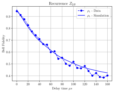
(a)

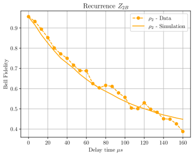
(b)

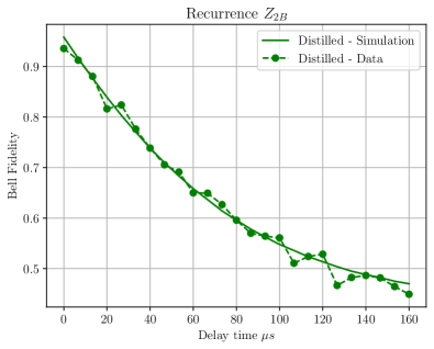
(c)

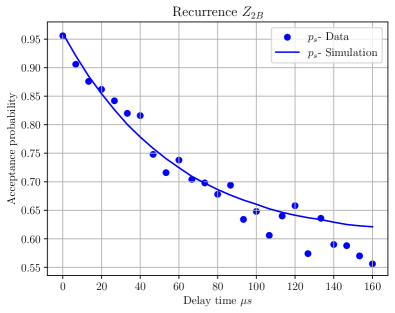
(d)

Figure 16: $Z_{2B}$ Recurrence distillation on qubits [0,1,2,3] of ibm_kyiv (points). Here simulations fit the data well. Solid lines are simulations assuming reported noise parameters as described in Table. 3 of App. E

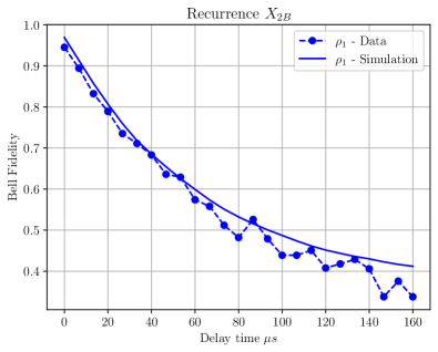
(a)

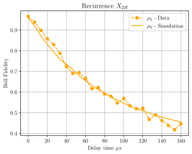
(b)

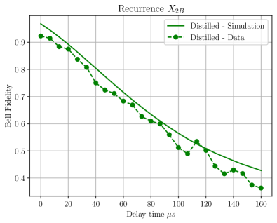
(c)

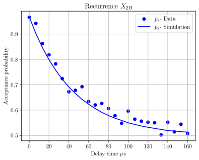
(d)

Figure 17: $X_{2B}$ distillation on qubits [0,1,2,3] of ibm_kyiv (points). Solid lines are simulations assuming reported noise parameters as described in Table. 4 of App. E

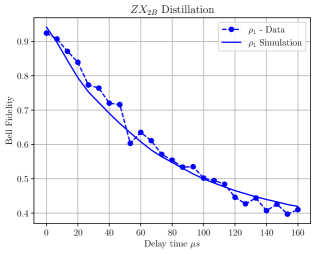
(a)

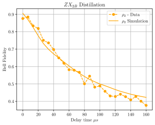
(b)

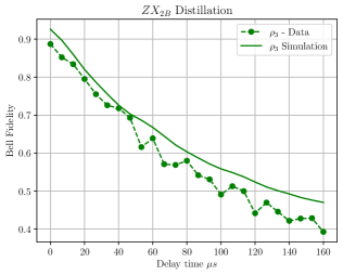
(c)

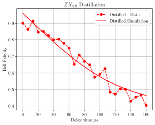
(d)

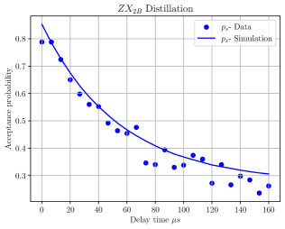
(e)

Figure 18: Bell fidelity as a function of time for pairs before and after carrying out $ZX_{3B}$ distillation on qubits $[3,4,5,6,7,8]$. Simulations assume reported noise parameters as described in Table. 5 and 6 of App. E

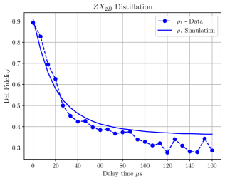
(a)

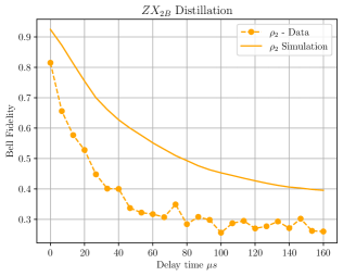
(b)

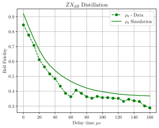
(c)

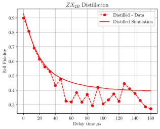
(d)

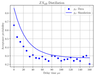
(e)

Figure 19: Bell fidelity as a function of time for pairs before and after carrying out $ZX_{3B}$ distillation on qubits $[59,60,61,62,63,64]$. Simulations assume reported noise parameters as described in Table. 5 and 6 of App. E

References

- Bennett et al. [1996a] C. H. Bennett, G. Brassard, S. Popescu, B. Schumacher, J. A. Smolin, and W. K. Wootters, Purification of Noisy Entanglement and Faithful Teleportation via Noisy Channels, Physical Review Letters 76, 722 (1996a), arXiv:quant-ph/9511027.
- Bennett et al. [1996b] C. H. Bennett, D. P. DiVincenzo, J. A. Smolin, and W. K. Wootters, Mixed-state entanglement and quantum error correction, Physical Review A 54, 3824 (1996b).
- Dür et al. [1999] W. Dür, H.-J. Briegel, J. I. Cirac, and P. Zoller, Quantum repeaters based on entanglement purification, Physical Review A 59, 169 (1999), arXiv:quant-ph/9808065.
- Gidney [2023] C. Gidney, Tetrationally compact entanglement purification (2023), arXiv:2311.10971 [quant-ph] .
- Shor [1996] P. Shor, Fault-tolerant quantum computation, in Proceedings of 37th Conference on Foundations of Computer Science (1996) pp. 56–65.
- Knill [2005] E. Knill, Scalable quantum computing in the presence of large detected-error rates, Phys. Rev. A 71, 042322 (2005).
- Bravyi et al. [2016] S. Bravyi, G. Smith, and J. A. Smolin, Trading classical and quantum computational resources, Phys. Rev. X 6, 021043 (2016).
- Kim et al. [2024] J. Kim, J. Yun, and J. Bae, Purification of Noisy Measurements and Faithful Distillation of Entanglement (2024), arXiv:2404.10538 [quant-ph].
- Shi et al. [2024] Y. Shi, C. Liu, S. Stein, M. Wang, M. Zheng, and A. Li, Design of an entanglement purification protocol selection module (2024), arXiv:2405.02555 [quant-ph].
- Yan et al. [2023] P. Yan, L. Zhou, W. Zhong, and Y. Sheng, Advances in quantum entanglement purification, Science China Physics, Mechanics & Astronomy 66, 250301 (2023), arXiv:2304.12679 [quant-ph].
- Kang et al. [2023] A. Kang, S. Guha, N. Rengaswamy, and K. P. Seshadreesan, Trapped ion quantum repeaters with entanglement distillation based on quantum ldpc codes, in 2023 IEEE International Conference on Quantum Computing and Engineering (QCE), Vol. 01 (2023) pp. 1165–1171.
- Miguel-Ramiro et al. [2023] J. Miguel-Ramiro, F. Riera-Sàbat, and W. Dür, Quantum repeater for states, PRX Quantum 4, 040323 (2023).
- Vandré and Gühne [2023] L. Vandré and O. Gühne, Entanglement Purification of Hypergraph States (2023), arXiv:2301.11341 [quant-ph].
- Devulapalli et al. [2022] D. Devulapalli, E. Schoute, A. Bapat, A. M. Childs, and A. V. Gorshkov, Quantum Routing with Teleportation (2022), arXiv:2204.04185 [quant-ph].
- Jansen et al. [2022] S. Jansen, K. Goodenough, S. de Bone, D. Gijswijt, and D. Elkouss, Enumerating all bilocal Clifford distillation protocols through symmetry reduction, Quantum 6, 715 (2022), arXiv:2103.03669 [quant-ph].
- Miguel-Ramiro and Dür [2018] J. Miguel-Ramiro and W. Dür, Efficient entanglement purification protocols for d-level systems, Physical Review A 98, 042309 (2018), arXiv:1806.10162 [quant-ph].
- Fujii and Yamamoto [2009] K. Fujii and K. Yamamoto, Entanglement Purification with Double Selection, Physical Review A 80, 042308 (2009), arXiv:0811.2639 [quant-ph].
- Glancy et al. [2006] S. Glancy, E. Knill, and H. M. Vasconcelos, Entanglement Purification of Any Stabilizer State, Physical Review A 74, 032319 (2006), arXiv:quant-ph/0606125.
- Aschauer and Briegel [2002] H. Aschauer and H. Briegel, Entanglement purification with noisy apparatus can be used to factor out an eavesdropper, The European Physical Journal D - Atomic, Molecular and Optical Physics 18, 171 (2002).
- Pan et al. [2001a] J.-W. Pan, C. Simon, Č. Brukner, and A. Zeilinger, Entanglement purification for quantum communication, Nature 410, 1067 (2001a).
- Pattison et al. [2024] C. A. Pattison, G. Baranes, J. P. B. Ataides, M. D. Lukin, and H. Zhou, Fast quantum interconnects via constant-rate entanglement distillation (2024), arXiv:2408.15936 [quant-ph] .
- Shi et al. [2025a] Y. Shi, A. Patil, and S. Guha, Stabilizer entanglement distillation and efficient fault-tolerant encoders, PRX Quantum 6, 010339 (2025a).
- Shi et al. [2025b] Y. Shi, A. Patil, and S. Guha, Measurement-based entanglement distillation and constant-rate quantum repeaters over arbitrary distances (2025b), arXiv:2502.11174 [quant-ph] .
- Briegel et al. [1998] H.-J. Briegel, W. Dür, J. I. Cirac, and P. Zoller, Quantum repeaters for communication (1998), arXiv:quant-ph/9803056.
- Hu et al. [2021a] X.-M. Hu, C.-X. Huang, Y.-B. Sheng, L. Zhou, B.-H. Liu, Y. Guo, C. Zhang, W.-B. Xing, Y.-F. Huang, C.-F. Li, and G.-C. Guo, Long-distance entanglement purification for quantum communication, Physical Review Letters 126, 010503 (2021a), arXiv:2101.07441 [quant-ph].
- Stein et al. [2023] S. Stein, S. Sussman, T. Tomesh, C. Guinn, E. Tureci, S. F. Lin, W. Tang, J. Ang, S. Chakram, A. Li, M. Martonosi, F. T. Chong, A. A. Houck, I. L. Chuang, and M. A. DeMarco, Microarchitectures for Heterogeneous Superconducting Quantum Computers (2023), arXiv:2305.03243 [quant-ph].
- Ang et al. [2022] J. Ang, G. Carini, Y. Chen, I. Chuang, M. A. DeMarco, S. E. Economou, A. Eickbusch, A. Faraon, K.-M. Fu, S. M. Girvin, M. Hatridge, A. Houck, P. Hilaire, K. Krsulich, A. Li, C. Liu, Y. Liu, M. Martonosi, D. C. McKay, J. Misewich, M. Ritter, R. J. Schoelkopf, S. A. Stein, S. Sussman, H. X. Tang, W. Tang, T. Tomesh, N. M. Tubman, C. Wang, N. Wiebe, Y.-X. Yao, D. C. Yost, and Y. Zhou, Architectures for Multinode Superconducting Quantum Computers (2022), arXiv:2212.06167 [quant-ph].
- Rozpȩdek et al. [2018] F. Rozpȩdek, T. Schiet, L. P. Thinh, D. Elkouss, A. C. Doherty, and S. Wehner, Optimizing practical entanglement distillation, Physical Review A 97, 062333 (2018), arXiv:1803.10111 [quant-ph].
- Krastanov et al. [2019] S. Krastanov, V. V. Albert, and L. Jiang, Optimized Entanglement Purification, Quantum 3, 123 (2019), arXiv:1712.09762 [quant-ph].
- Victora et al. [2023] M. Victora, S. Tserkis, S. Krastanov, A. S. De La Cerda, S. Willis, and P. Narang, Entanglement purification on quantum networks, Physical Review Research 5, 033171 (2023).
- Zhao et al. [2021] X. Zhao, B. Zhao, Z. Wang, Z. Song, and X. Wang, Practical distributed quantum information processing with LOCCNet, npj Quantum Information 7, 159 (2021).
- Kwiat et al. [2001] P. G. Kwiat, S. Barraza-Lopez, A. Stefanov, and N. Gisin, Experimental entanglement distillation and ‘hidden’ non-locality, Nature 409, 1014 (2001).
- Pan et al. [2003a] J.-W. Pan, S. Gasparoni, R. Ursin, G. Weihs, and A. Zeilinger, Experimental entanglement purification of arbitrary unknown states, Nature 423, 417 (2003a).
- Pan et al. [2001b] J.-W. Pan, C. Simon, Č. Brukner, and A. Zeilinger, Entanglement purification for quantum communication, Nature 410, 1067 (2001b).
- Pan et al. [2003b] J.-W. Pan, S. Gasparoni, R. Ursin, G. Weihs, and A. Zeilinger, Experimental entanglement purification of arbitrary unknown states, Nature 423, 417 (2003b).
- Yamamoto et al. [2003] T. Yamamoto, M. Koashi, Ş. K. Özdemir, and N. Imoto, Experimental extraction of an entangled photon pair from two identically decohered pairs, Nature 421, 343 (2003).
- Dong et al. [2008] R. Dong, M. Lassen, J. Heersink, C. Marquardt, R. Filip, G. Leuchs, and U. L. Andersen, Experimental entanglement distillation of mesoscopic quantum states, Nature Physics 4, 919 (2008).
- Chen et al. [2017] L.-K. Chen, H.-L. Yong, P. Xu, X.-C. Yao, T. Xiang, Z.-D. Li, C. Liu, H. Lu, N.-L. Liu, L. Li, T. Yang, C.-Z. Peng, B. Zhao, Y.-A. Chen, and J.-W. Pan, Experimental nested purification for a linear optical quantum repeater, Nature Photonics 11, 695 (2017).
- Hu et al. [2021b] X.-M. Hu, C.-X. Huang, Y.-B. Sheng, L. Zhou, B.-H. Liu, Y. Guo, C. Zhang, W.-B. Xing, Y.-F. Huang, C.-F. Li, and G.-C. Guo, Long-distance entanglement purification for quantum communication, Phys. Rev. Lett. 126, 010503 (2021b).
- Reichle et al. [2006] R. Reichle, D. Leibfried, E. Knill, J. Britton, R. B. Blakestad, J. D. Jost, C. Langer, R. Ozeri, S. Seidelin, and D. J. Wineland, Experimental purification of two-atom entanglement, Nature 443, 838 (2006).
- Kalb et al. [2017] N. Kalb, A. A. Reiserer, P. C. Humphreys, J. J. W. Bakermans, S. J. Kamerling, N. H. Nickerson, S. C. Benjamin, D. J. Twitchen, M. Markham, and R. Hanson, Entanglement distillation between solid-state quantum network nodes, Science 356, 928 (2017).
- Yan et al. [2022] H. Yan, Y. Zhong, H.-S. Chang, A. Bienfait, M.-H. Chou, C. R. Conner, E. Dumur, J. Grebel, R. G. Povey, and A. N. Cleland, Entanglement Purification and Protection in a Superconducting Quantum Network, Physical Review Letters 128, 080504 (2022).
- Qin et al. [2023] H. Qin, M.-M. Du, X.-Y. Li, W. Zhong, L. Zhou, and Y.-B. Sheng, Efficient multipartite entanglement purification with non-identical states (2023), arXiv:2311.10250 [quant-ph].
- Aliferis et al. [2009] P. Aliferis, F. Brito, D. P. DiVincenzo, J. Preskill, M. Steffen, and B. M. Terhal, Fault-tolerant computing with biased-noise superconducting qubits: a case study, New Journal of Physics 11, 013061 (2009).
- Siddhu et al. [2024] V. Siddhu, D. Abdelhadi, T. Jochym-O’Connor, and J. Smolin, Entanglement sharing across a damping-dephasing channel (2024), arXiv:2405.06231 [quant-ph] .
- Emerson et al. [2005] J. Emerson, R. Alicki, and K. Życzkowski, Scalable noise estimation with random unitary operators, Journal of Optics B: Quantum and Semiclassical Optics 7, S347–S352 (2005).
- Dankert et al. [2009] C. Dankert, R. Cleve, J. Emerson, and E. Livine, Exact and approximate unitary 2-designs and their application to fidelity estimation, Phys. Rev. A 80, 012304 (2009).
- Gupta et al. [2024] R. S. Gupta, N. Sundaresan, T. Alexander, C. J. Wood, S. T. Merkel, M. B. Healy, M. Hillenbrand, T. Jochym-O’Connor, J. R. Wootton, T. J. Yoder, A. W. Cross, M. Takita, and B. J. Brown, Encoding a magic state with beyond break-even fidelity, Nature 625, 259 (2024).
- Proctor et al. [2022] T. Proctor, S. Seritan, K. Rudinger, E. Nielsen, R. Blume-Kohout, and K. Young, Scalable randomized benchmarking of quantum computers using mirror circuits, Phys. Rev. Lett. 129, 150502 (2022).
- Zhou et al. [2023] Z. Zhou, R. Sitler, Y. Oda, K. Schultz, and G. Quiroz, Quantum crosstalk robust quantum control, Phys. Rev. Lett. 131, 210802 (2023).
- Shirizly et al. [2024] L. Shirizly, G. Misguich, and H. Landa, Dissipative dynamics of graph-state stabilizers with superconducting qubits, Phys. Rev. Lett. 132, 010601 (2024).
- Seif et al. [2024] A. Seif, H. Liao, V. Tripathi, K. Krsulich, M. Malekakhlagh, M. Amico, P. Jurcevic, and A. Javadi-Abhari, Suppressing correlated noise in quantum computers via context-aware compiling, in 2024 ACM/IEEE 51st Annual International Symposium on Computer Architecture (ISCA) (IEEE, 2024) p. 310–324.
- Jurcevic and Govia [2022] P. Jurcevic and L. C. G. Govia, Effective qubit dephasing induced by spectator-qubit relaxation, Quantum Science and Technology 7, 045033 (2022).
- Ambainis and Gottesman [2006] A. Ambainis and D. Gottesman, The minimum distance problem for two-way entanglement purification, IEEE Transactions on Information Theory 52, 748 (2006).
- Shor and Smolin [1996] P. W. Shor and J. A. Smolin, Quantum error-correcting codes need not completely reveal the error syndrome (1996), arXiv:quant-ph/9604006 [quant-ph] .