Functional Itô-formula and Taylor expansions
for non-anticipative maps of càdlàg rough paths

Abstract

We derive a functional Itô-formula for non-anticipative maps of rough paths, based on the approximation properties of the signature of càdlàg rough paths. This result is a functional extension of the Itô-formula for càdlàg rough paths (by Friz and Zhang (2018)), which coincides with the change of variable formula formulated by Dupire (2009) whenever the functionals’ representations, the notions of regularity, and the integration concepts can be matched. Unlike these previous works, we treat the vertical (jump) pertubation via the Marcus transformation, which allows for incorporating path functionals where the second order vertical derivatives do not commute, as is the case for typical signature functionals. As a byproduct, we show that sufficiently regular non-anticipative maps admit a functional Taylor expansion in terms of the path’s signature, leading to an important generalization of the recent results by Dupire and Tissot-Daguette (2022).

Keywords: càdlàg rough paths, signature, functional Itô-formula, Taylor expansion of path functionals in terms of signature, universal approximation theorem
MSC (2020) Classification: 60L20, 60L10

1 Introduction

The Itô-formula is one of the major tools of stochastic calculus, extending the chain rule from classical calculus to stochastic analysis and asserting that any sufficiently smooth function of a semimartingale is itself a semimartingale. Recognizing that the functional dependence on a stochastic system does not only occur through its current state but also through its entire history, the seminal papers by Dupire (2009, 2019) and Cont and Fournie (2010a, b) extend the Itô-formula to non-anticipative path functionals, which may depend on the past trajectory of a $\mathbb{R}^{d}$-valued semimartingale up to the present time. These works have led to many subsequent contributions, including Cont and Fournie (2013), Litterer and Oberhauser (2011),  Keller and Zhang (2016), Ananova and Cont (2017), Cont and Perkowski (2018), Viens and Zhang (2019), Houdré and Víquez (2024), and the references therein.

The original formulation of the functional Itô-formula incorporates vertical and horizontal derivatives, reflecting the functional’s dependence on the trajectory and current time, respectively (see Section 2 in Dupire (2009)). This formula is derived using a Taylor expansion of the functional along an approximation of the path, leading to a second-order approximation, which is quadratic in the path increments and thus involves the semimartingale’s quadratic variation in the limit. It is therefore not surprising that this technique may not only be applied to functionals of semimartingales but also to more general paths of finite quadratic variation. This is in fact the finding of the paper Cont and Fournie (2013), which establishes a pathwise functional Itô-formula for non-anticipative functionals of càdlàg paths of finite quadratic variation in the sense of Föllmer (1981). Other forms of generalizations can also be found in Oberhauser (2016), which builds on Bichteler (1981).

Even though these results cover a wide range of pratically relevant path functionals, certain important classes of interest are still excluded. Indeed, their framework is limited to functionals that depend continuously on the trajectories of the path with respect to (some variants of) the uniform topology (see e.g., Section 1.2 in Cont and Fournie (2013)). This excludes several crucial examples, such as the Itô-map, which describes the correspondence between the solution of a stochastic differential equation and the driving signal, or standard Itô/Stratonovich integrals. To see this, consider, for instance, the sequence of real-valued paths $X^{1,n},X^{2,n}:[0,2\pi]\rightarrow\mathbb{R}$ defined via

$$X^{1,n}_{t}:=-n^{-\frac{1}{3}}\cos(nt),\qquad X^{2,n}_{t}:=n^{-\frac{1}{3}}\sin(nt),\qquad\text{for all }t\in[0,2\pi],$$

for $n\in\mathbb{N}$. Then,

$$\int_{0}^{2\pi}X^{2,n}_{s}dX^{1,n}_{s}=n^{\frac{1}{3}}\pi,$$ (1.1)

implying that $X^{1,n},X^{2,n}\rightarrow 0$ in the uniform topology, but $\int_{0}^{2\pi}X^{2,n}_{s}dX^{1,n}_{s}\rightarrow\infty$, (see Allan (2021)), showing that iterated integrals are not continuous with respect to the uniform topology. These topological limitations raise the question of defining a suitable topology on the space of paths to enable a more general applicability of a (pathwise) functional Itô-formula.

Our approach is inspired by the theory of rough paths, pioneered by Terry Lyons (see Lyons (1998); Lyons et al. (2007)), where one of the fundamental results consists of identifying a natural family of topologies on path space so that iterated Stratonovich and Itô-integrals, and more generally solutions to controlled differential equations, are continuous maps with respect to the driving signal. Relying on this idea, we thus equip the path spaces with a (stronger) variation topology (Definition 2.10) and consider functionals of weakly geometric càdlàg $p$-rough paths for $p\in[1,3)$ (Definition 2.1). This means that when dealing with paths of finite $p$-variation for $p\geq 2$, which is the case for sample paths of a semimartingale, we consider functionals that depend on a lifted path, i.e., the $\mathbb{R}^{d}$-valued path itself and (some of) its rough path lift. In this setup we establish a pathwise functional Itô-formula for càdlàg rough paths that covers the above examples. With this approach we can also treat functionals that just depend on the path itself (and not necessarily on its lift) as in the settings of Dupire (2009) and Cont and Fournie (2010a, b).

Our proof technique is based on a density approach building on linear functions of the signature (Section 3.4), which are in fact specific non-anticipative functionals of weakly geometric rough paths that exhibit powerful approximating properties (see e.g., Section 3 in Cuchiero et al. (2025) as well as Kalsi et al. (2020), Bayer et al. (2023), Cuchiero et al. (2023)). Specifically, we first establish an Itô-formula for these specific functionals and then extend it to more general maps via a density argument. This proof technique has also been used in classical stochastic calculus (see, e.g., Theorem 5.7 in Miller and Silvestri (2017)), as well as for measure-valued processes (see, e.g., Guo et al. (2023), Jacka and Tribe (2003)), relying on density results for certain classes of cylindrical functions.

The key component to make this approach work in the current setup is an appropriate form of a Nachbin-type universal approximation theorem (UAT) (see Nachbin (1949)) for functionals of weakly geometric càdlàg $p$-rough paths for $p\in[1,3)$ and certain derivatives thereof (Theorem 4.14). In this respect there are two crucial concepts that need to be developed, namely, non-anticipative Marcus canonical path functionals, and their vertical derivatives.

First, inspired by Chevyrev and Friz (2019) (see also Marcus (1978, 1981) and Williams (2001)) and in particular by the construction of the signature of càdlàg paths (Section 2.5), we introduce the class of non-anticipative Marcus canonical path functionals. Roughly speaking, these are maps

$$F:[0,1]\times D([0,1],G^{[p]}(\mathbb{R}^{d}))\rightarrow\mathbb{R},$$

which depend on weakly geometric càdlàg rough paths (denoted by $D([0,1],G^{[p]}(\mathbb{R}^{d})$) in a non anticipative way (Definition 3.2) and which are invariant under the Marcus transformation, i.e.,

$$F(t,\mathbf{X})=F(\psi_{R}^{-1}(\tau_{\mathbf{X},R}(t)),\widetilde{\mathbf{X}}),$$

for $\widetilde{\mathbf{X}}$ denoting the Marcus transformed path of $\mathbf{X}$ with respect to some pair $(R,\psi_{R})$. More precisely, $\widetilde{\mathbf{X}}$ denotes the continuous path obtained by interpolating the states before and after each jump time of $\mathbf{X}$ via the log-linear path-function and satisfying $\widetilde{\mathbf{X}}_{\psi_{R}^{-1}(\tau_{\mathbf{X},R}(\cdot))}=\mathbf{X}_{\cdot}$ (see Section 2.4 and Definition 3.4 for the precise definition of the involved quantities, and also  Fujiwara and Kunita (1985), Applebaum and Tang (2001), Kurtz et al. (1995), and Chevyrev et al. (2020) where a similar approach is used).

Second, viewing weakly geometric rough paths as (free step-$[p]$ nilpotent) Lie group valued paths, we introduce a notion of vertical derivatives for Marcus canonical paths functionals, inspired by the (Euclidean) one introduced in Dupire (2009). We call the quantity

$$U^{i}F(t,\mathbf{X}):=\frac{d}{dh}F(\psi_{R}^{-1}(\tau_{\mathbf{X},R}(t)),\widetilde{\mathbf{X}}\otimes\exp^{([p])}(h\epsilon_{i})1_{\{\cdot\geq\psi_{R}^{-1}(\tau_{\mathbf{X},R}(t)\}})|_{h=0},$$ (1.2)

vertical derivative of $F$ in the direction $i=1,\dots,d$ at $(t,\mathbf{X})$, whenever it exists (Definition 3.13). Notice that (1.2) might be interpreted as a directional derivative of the functional in the direction determined by the vertical perturbation $\exp^{([p])}(h\epsilon_{i})1_{\{\cdot\geq\psi_{R}^{-1}(\tau_{\mathbf{X},R}(t)\}}$, which is designed to stay in the Lie group and where $\epsilon_{i}$ denotes the $i$-th canonical basis vector of $\mathbb{R}^{d}$. This is conceptually consistent with Qian and Tudor (2011), where a first attempt for studying a differential structure of the (non-linear) space of rough paths has been made (see also Schmeding (2022) for a discussion on this topic).

A crucial aspect when inserting a càdlàg path in (1.2) is the following: the Marcus transformation of the path $\mathbf{X}$ needs to be computed before the vertical perturbation. On one hand, this preserves the Marcus property of the functional also on the level of the (functional) derivative (Proposition 3.15). On the other hand, if the original path $\mathbf{X}$ admits a jump at time $t$, the Marcus property of the functional $F$ allows to interpret the derivative in (1.2) as a derivative involving a delayed perturbation of the original path

$$\mathbf{X}^{t}\otimes\exp^{([p])}(h\epsilon_{i})1_{\{\cdot\geq t+\varepsilon\}},$$

for some $\varepsilon>0$ independent of the specific pair $(R,\psi_{R})$ (Remark 3.14(ii)). This specification is particularly relevant when computing the higher-order vertical derivatives, which is through an iterative application of the procedure in (1.2) (Definition 3.17). In this case, by definition, the perturbations are always computed at a jump time, resulting therefore in a notion of vertical derivatives of order $k\in\mathbb{N}$, $k\geq 2$, which involve delayed perturbations of the form

$$\mathbf{X}^{t}\otimes\exp^{([p])}(h_{k}\epsilon_{i_{k}})1_{\{\cdot\geq t+\varepsilon_{k}\}}\otimes\dots\otimes\exp^{([p])}(h_{1}\epsilon_{i_{1}})1_{\{\cdot\geq t+\varepsilon_{k}+\dots+\varepsilon_{1}\}},$$

for some $h_{k},\dots,h_{1}\in\mathbb{R}$, $\varepsilon_{k},\dots,\varepsilon_{1}>0$, and $i_{k},\dots,i_{1}=1,\dots,d$.

Relying on these two notions, we then establish the first main result of the paper, a universal approximation theorem (UAT) for vertically differentiable path functionals: any $C^{K}$-non-anticipative Marcus canonical path functionals $F$ (Definition 4.12) evaluated at some tracking jumps-extended path $\widehat{\mathbf{X}}$ (Definiton 4.4) can be approximated uniformly in time together with its derivatives by linear functionals of the signature and their derivatives (Theorem 4.14). Due to the non-linear structure of the vertical (Lie) derivatives, the proof of this result is highly delicate. Indeed, it is a tricky combination of Nachbin-type theorems (see Nachbin (1949)) and some key concepts from Lie group theory.

With the above notions of vertical derivatives, a functional Itô-formula for linear functions of the signature follows by the definition of the signature of weakly geometric càdlàg rough paths. Furthermore, the UAT for functionals of weakly geometric càdlàg $p$-rough paths, combined with some interpolation arguments, yields our second main result: a (rough) functional Itô-formula for the class of $C^{[p]+1}$ non-anticipative Marcus canonical path functional (Theorems 5.1, 5.4). Here, it is required that the functional itself, its derivatives, and a certain remainder (Definition 3.12) are continuous with respect to the above mentioned variation norms (Definition 3.21). We then also show that our Itô-formula matches some standard as well as functional Itô-formulas in the literature (see Section 5.3).

The last main result of the paper is the functional Taylor expansion in terms of the signature (Theorems 6.1, 6.3). To the best of our knowledge, this is the first purely deterministic (rough) Taylor expansion of functionals of weakly geometric càdlàg $p$-rough paths. It nevertheless shares similarities with the work by Buckdahn et al. (2015), where a rough Taylor expansion is derived by identifying the vertical derivatives with the abstract notion of Gubinelli derivatives, with expansions coming from control theory e.g., Fliess (1981, 1983, 1986), Beauchard et al. (2023), as well as stochastic Taylor expansions (see e.g., Litterer and Oberhauser (2011), Klöden and Platen (1992), Arous (1989)), and recent results in Dupire and Tissot-Daguette (2023).

Let us reiterate that the treatment via the Marcus transformation, which leads to non commutative higher order derivatives, is crucial for the Taylor expansion in terms of the signature components, which are non-symmetric tensors due to the non-commutativity of the iterated integrals. These results would not follow from a direct application of the differential calculus introduced in Dupire (2009) and Cont and Fournie (2010a) as the higher order functional derivatives always take values in the space of symmetric tensors over $\mathbb{R}^{d}$ (see e.g., Cont and Perkowski (2018), Bielert (2024) as well as Remarks 3.20 and 6.4(iii)).

Organization of the paper.

In Section 3, we introduce the space of non-anticipative Marcus canonical path functionals and the corresponding differential calculus, as well as the considered $p$-variation topologies. In Section 4, we introduce the set of “tracking-jumps-extended paths” and present the UAT for vertically differentiable path functionals. In Section 5 and Section 6, we prove the functional Itô-formula and the Taylor expansion, respectively. In the Appendix, we collect the technical proofs and some remarks on rough integration theory as well as different pathwise integration approaches to which we compare the current rough setting.

2 Preliminaries

2.1 Algebraic setting

Fix $d\in\mathbb{N}$ and let $\mathbb{R}^{d}$ be the Euclidean space. The extended tensor algebra over $\mathbb{R}^{d}$ is defined by

$$T((\mathbb{R}^{d})):=\{\mathbf{u}=(\mathbf{u}^{(0)},\mathbf{u}^{(1)},\dots,\mathbf{u}^{(n)},\dots)\ |\ \mathbf{u}^{(n)}\in\mathbb{R}^{\otimes n}\},$$

where $(\mathbb{R}^{d})^{\otimes n}$ denotes the $n$-fold tensor product of $\mathbb{R}^{d}$ with the convention $(\mathbb{R}^{d})^{\otimes 0}:=\mathbb{R}$. We equip $T((\mathbb{R}^{d}))$ with the standard addition $+$, tensor multiplication $\otimes$, and scalar multiplication. For $N\in\mathbb{N}$, the truncated tensor algebra is defined by

$$T^{N}(\mathbb{R}^{d}):=\{\mathbf{u}=(\mathbf{u}^{(0)},\mathbf{u}^{(1)},\dots,\mathbf{u}^{(N)})\ |\ \mathbf{u}^{(n)}\in\mathbb{R}^{\otimes n}\ \text{for }n\leq N\},$$

and the tensor algebra via $T(\mathbb{R}^{d}):=\bigcup_{N\in\mathbb{N}}T^{N}(\mathbb{R}^{d})$. Let $\pi_{n}:T((\mathbb{R}^{d}))\rightarrow(\mathbb{R}^{d})^{\otimes n}$ and $\pi_{\leq N}:T((\mathbb{R}^{d}))\rightarrow T^{N}(\mathbb{R}^{d})$ be the maps such that for $\mathbf{u}\in T((\mathbb{R}^{d})),$

$$\pi_{n}(\mathbf{u}):=\mathbf{u}^{(n)},\qquad\pi_{\leq N}(\mathbf{u}):=(\mathbf{u}^{(n)})_{n=0}^{N}.$$

For $c\in\mathbb{R}$, set

$$T^{N}_{c}(\mathbb{R}^{d}):=\{\mathbf{u}\in T^{N}(\mathbb{R}^{d})\colon\mathbf{u}^{(0)}=c\}.$$

The space $T_{1}^{N}(\mathbb{R}^{d})$ is a Lie group under the tensor multiplication $\otimes$, truncated beyond level $N$. The neutral element with respect to $\otimes$ is $\mathbf{1}:=(1,0,\dots,0)\in T_{1}^{N}(\mathbb{R}^{d})$. Moreover, for any $\mathbf{u}=(\mathbf{1}+\mathbf{b})\in T_{1}^{N}(\mathbb{R}^{d})$, with $\mathbf{b}\in T_{0}^{N}(\mathbb{R}^{d})$, its inverse is given by

$$\mathbf{u}^{-1}=\sum_{k=0}^{N}(-1)^{k}\mathbf{b}^{\otimes k}.$$ (2.1)

The exponential and logarithm maps are defined as follows:

$$\exp^{(N)}:T {}_{0}^{N}(\mathbb{R}^{d})\rightarrow T_{1}^{N}(\mathbb{R}^{d})\qquad\quad \log^{(N)}:T {}_{1}^{N}(\mathbb{R}^{d})\rightarrow T_{0}^{N}(\mathbb{R}^{d})$$ (2.2)

$$\mathbf{b}\mapsto\mathbf{1}+\sum_{k=1}^{N}\frac{\mathbf{b}^{\otimes k}}{k!},\qquad \mathbf{1}+\mathbf{\mathbf{b}}\mapsto\sum_{k=1}^{N}(-1)^{k+1}\frac{\mathbf{b}^{\otimes k}}{k},$$

where the tensor multiplication is again always truncated beyond level $N$. We furthermore introduce the (non-truncated) exponential map, which is given by

$$\exp({\mathbf{u}}):=1+\sum_{k=1}^{\infty}\frac{\mathbf{u}^{\otimes k}}{k!}\in T((\mathbb{R}^{d+1})),$$ (2.3)

for each $\mathbf{u}\in T((\mathbb{R}^{d+1}))$ such that $\pi_{0}(\mathbf{u})=0$. Let $\mathfrak{g}^{N}(\mathbb{R}^{d})$ be the free step-$N$ nilpotent Lie algebra over $\mathbb{R}^{d}$, i.e.,

$$\mathfrak{g}^{N}(\mathbb{R}^{d}):=\{0\}\oplus\mathbb{R}^{d}\oplus[\mathbb{R}^{d},\mathbb{R}^{d}]\oplus\dots\oplus\underbrace{[\mathbb{R}^{d},[\mathbb{R}^{d},\dots,[\mathbb{R}^{d},\mathbb{R}^{d}]]]}_{(N-1)\text{ brackets}}\subseteq T_{0}^{N}(\mathbb{R}^{d}),$$ (2.4)

where, for $\mathbf{u}\in T_{0}^{M}(\mathbb{R}^{d})$, $1\leq M\leq N-1$, $\mathbf{b}^{(1)}\in\mathbb{R}^{d}$, $[\mathbf{b}^{(1)},\mathbf{u}]:=\mathbf{b}^{(1)}\otimes\mathbf{u}-\mathbf{u}\otimes\mathbf{b}^{(1)}$.

The image of $\mathfrak{g}^{N}(\mathbb{R}^{d})$ through the exponential map is a subgroup of $T_{1}^{N}(\mathbb{R}^{d})$ with respect to $\otimes$. It is called free step-$N$ nilpotent Lie group and is denoted by

$$G^{N}(\mathbb{R}^{d}):=\exp^{(N)}(\mathfrak{g}^{N}(\mathbb{R}^{d})).$$ (2.5)

We equip it with the so-called Carnot-Caratheodory (CC) norm $\|\cdot\|_{CC}$ (see Definition and Theorem 7.32 in Friz and Victoir (2010)) and the induced (left-invariant) metric, denoted by $d_{CC}$ (see Definition 7.41 in Friz and Victoir (2010)). Finally, we introduce the set of so-called group-like elements, defined via

$$G((\mathbb{R}^{d})):=\{\mathbf{x}\in T((\mathbb{R}^{d}))\ |\ \pi_{\leq N}(\mathbf{x})\in G^{N}(\mathbb{R}^{d})\text{ for all }N\}.$$ (2.6)

We refer to Chapter 7 in Friz and Victoir (2010) for more details on these algebraic aspects and the specific group $G^{N}(\mathbb{R}^{d})$ (see also Section 2 in Lyons et al. (2007)), and to Bonfiglioli et al. (2007) and Schmeding (2022) for a more general treatment of Lie groups.

Let $I=(i_{1},\dots,i_{n})$ be a multi-index with entries in $\{1,\dots,d\}$. Denoting by $\epsilon_{1},\ldots,\epsilon_{d}$ the canonical basis of $\mathbb{R}^{d}$, we use the notation $|I|:=n$ and $\epsilon_{I}:=\epsilon_{i_{1}}\otimes\epsilon_{i_{2}}\otimes\dots\otimes\epsilon_{i_{n}}$. Observe that $(\epsilon_{I})_{I}$ is the canonical orthonormal basis of $(\mathbb{R}^{d})^{\otimes n}$. Furthermore, we denote by $\epsilon_{\emptyset}$ the basis element of $(\mathbb{R}^{d})^{\otimes 0}$ and set $|\emptyset|:=0$. We also set $I^{\prime}:=(i_{1},\dots,i_{n-1})$ for $n>1$, ${I^{\prime}}=\emptyset$ for $n=1$, $I^{{}^{\prime\prime}}:=(I^{\prime})^{\prime}$ for $n>1$, and use the convention $\epsilon_{I^{\prime\prime}}=0$ for $n=1$. Given $\mathbf{x}\in T((\mathbb{R}^{d})),$ we write $\mathbf{x}_{I}:=\langle\mathbf{x},\epsilon_{I}\rangle$ and for each ${\mathbf{u}\in T(\mathbb{R}^{d})}$, we set

$$\langle\mathbf{u},\mathbf{x}\rangle:=\sum_{|I|\geq 0}\mathbf{u}_{I}\mathbf{x}_{I}\in\mathbb{R}.$$

For $k\in\mathbb{N}$, we denote by $({\,\cdot\,})^{(k)}:T((\mathbb{R}^{d}))\to(T((\mathbb{R}^{d})))^{\otimes k}$ the shifts given by

$$\mathbf{u}^{(k)}_{I}:=\sum_{|J|\geq 0}\mathbf{u}_{JI}\epsilon_{J},$$ (2.7)

for each $|I|=k$, where $JI$ denotes the concatenation of the multi-indices $J$ and $I$. We also write $\mathbf{u}^{(0)}:=\mathbf{u}$ for notational convenience.

For two multi-indices $I\in\{1,\dots,d\}^{|I|}$, $J\in\{1,\dots,d\}^{|J|}$, and $a,b\in\{1,\dots,d\}$, the shuffle product $\shuffle$ is defined recursively by

$$I\shuffle\emptyset=\emptyset\shuffle I=I,$$

$$(I,a)\shuffle(J,b)=((I\shuffle(J,b)),a)+(((I,a)\shuffle J),b),$$

where $(I,a)$ denotes the concatenation of the multi-index $I$ with the element $a$.

Via the shuffle product, every polynomial on the set of group-like elements $G((\mathbb{R}^{d}))$ admits a linear representative. More precisely, for $\mathbf{x}\in G((\mathbb{R}^{d}))$ and two multi-indices $I\in\{1,\dots,d\}^{|I|}$, $J\in\{1,\dots,d\}^{|J|}$, it holds that

$$\langle\epsilon_{I},\mathbf{x}\rangle\langle\epsilon_{J},\mathbf{x}\rangle=\langle\epsilon_{I}\shuffle\epsilon_{J},\mathbf{x}\rangle,$$ (2.8)

where $\epsilon_{I}\shuffle\epsilon_{J}:=\sum_{k=1}^{K}\epsilon_{I_{k}}$ with $K,I_{k}$ for $k=1,\ldots,K$ determined via $I\shuffle J=\sum_{k=1}^{K}I_{k}$.

2.2 Weakly geometric càdlàg rough paths

Throughout, we denote by $C([0,1],E)$ and $D([0,1],E)$ the space of continuous and càdlàg maps (paths), respectively, from the interval $[0,1]$ into a metric space $(E,d)$ equipped with metric $d$. For $t\in(0,1]$, we denote a partition of $[0,t]$ by $\pi_{[0,t]}=\{0=t_{0}<t_{1}<\dots<t_{k}=t\}$, and write $\sum_{t_{i}\in\pi_{[0,t]}}$ for the summation over all points in $\pi_{[0,t]}$. The mesh size of $\pi_{[0,t]}$ is given by $|\pi_{[0,t]}|:=\max\{t_{i+1}-t_{i}\ :\ i=0,\dots,k-1\}$. For $p>0$, we define the $p$-variation of a path $X\in D([0,1],E)$ by

$$\|X\|_{p\text{-}var}:=\sup_{\pi_{[0,1]}\subset[0,1]}\left(\sum_{t_{i}\in\pi_{[0,t]}}d(X_{t_{i}},X_{t_{i+1}})^{p}\right)^{\frac{1}{p}}.$$ (2.9)

If $X$ takes values in a vector space, for $s,t\in[0,1]$, $s\leq t$, we use the shortcut $X_{s,t}:=X_{t}-X_{s}$ and denote the jumps by $\Delta X_{t}:=\lim_{s\nnearrow t}X_{s,t}$. The space of continuous and càdlàg paths of finite $p$-variation are denoted respectively by $C^{p}([0,1],E)$ and $D^{p}([0,1],E)$. We endow these spaces with the $p$-variation pseudometric, defined via

$$d_{p}(X,Y):=\sup_{\pi_{[0,1]}\subset[0,1]}\left(\sum_{t_{i}\in\pi_{[0,1]}}d(X_{t_{i},t_{i+1}},Y_{t_{i},t_{i+1}})^{p}\right)^{\frac{1}{p}},$$ (2.10)

for all $X,Y\in D^{p}([0,1],E)$. Additionally, we also consider two-parameter functions $A:\Delta_{1}\rightarrow V$, where $(V,\|\cdot\|)$ is a normed vector space and $\Delta_{1}:=\{(s,t)\in[0,1]\times[0,1]\ :\ s\leq t\}$. Analogously to paths, the notion of $p$-variation is valid for such functions and defined as

$$\|A\|_{p\text{-}var}:=\sup_{\pi_{[0,1]}\subset[0,1]}\left(\sum_{t_{i}\in\pi_{[0,1]}}\|A_{t_{i},t_{i+1}}\|^{p}\right)^{\frac{1}{p}}.$$

Similarly, we set $d_{p}(A,A^{\prime}):=\|A-A^{\prime}\|_{p\text{-}var}$ for all $A,A^{\prime}:\Delta_{1}\rightarrow V$ for which $\|A\|_{p},\|A^{\prime}\|_{p}<\infty$. We write $\|\cdot\|$ to denote the norm on any vector space $V$ that may differ from case to case.

We say that a path $X\in D([0,1],E)$ is a time-reparametrization of some $Y\in D([0,1],E)$ if $Y=X_{\phi}$, for some $\phi$ time-reparametrization, i.e., $\phi:[0,1]\rightarrow[0,1]$ is increasing and bijective.

Let $C([0,1],G^{N}(\mathbb{R}^{d}))$ and $D([0,1],G^{N}(\mathbb{R}^{d}))$ be the space of continuous and càdlàg maps (paths), respectively, from the interval $[0,1]$ into $(G^{N}(\mathbb{R}^{d}),d_{CC})$. For $\mathbf{X}\in D([0,1],G^{N}(\mathbb{R}^{d}))$, $s,t\in[0,1]$, $s\leq t$, the path increments are defined via

$$\mathbf{X}_{s,t}:=\mathbf{X}_{s}^{-1}\otimes\mathbf{X}_{t}$$ (2.11)

and the jumps by $\Delta\mathbf{X}_{t}:=\lim_{s\nnearrow t}\mathbf{X}_{s,t}$. For $p>0$, we denote by $[p]$ its entire part. Càdlàg paths of finite $p$-variation with values in the specific group $G^{[p]}(\mathbb{R}^{d})$ are called weakly geometric $p$-rough path. We formalize this notion in the definition below.

We restrict the presentation only to paths of finite $p$-variation for $p\in[1,3)$, which are the most relevant in the settings of stochastic analysis.

Definition 2.1.

Let $p\in[1,3)$. A càdlàg path $\mathbf{X}:[0,1]\rightarrow G^{[p]}(\mathbb{R}^{d})$ is a weakly geometric càdlàg $p$-rough path over $\mathbb{R}^{d}$ if $\|\mathbf{X}\|_{p\text{-}var}<\infty.$ We denote the space of such paths by $D^{p}([0,1],G^{[p]}(\mathbb{R}^{d}))$ and its subspace consisting of continuous paths by $C^{p}([0,1],G^{[p]}(\mathbb{R}^{d}))$.

For $p\in[2,3)$, $\mathbf{X}\in D^{p}([0,1],G^{[p]}(\mathbb{R}^{d}))$ is Marcus-like if for all $t\in[0,1]$,

$$\log^{(2)}(\Delta\mathbf{X}_{t})\in\{0\}\oplus\mathbb{R}^{d}\oplus\{0\}.$$

Assumption 2.2.

Unless otherwise specified, in this paper, we always assume $p\in[1,3)$.

Finally, we introduce the notion of a controlled rough path with respect to $X:=\pi_{1}(\mathbf{X})$, for some $\mathbf{X}\in D^{p}([0,1],G^{2}(\mathbb{R}^{d}))$ with $p\in[2,3)$. Let $\mathcal{L}(\mathbb{R}^{d},\mathbb{R}^{m})$ denote the space of linear maps from $\mathbb{R}^{d}$ into $\mathbb{R}^{m}$, for some $m\in\mathbb{N}$.

Definition 2.3.

Fix $p\in[2,3)$ and $\mathbf{X}\in D^{p}([0,1],G^{2}(\mathbb{R}^{d}))$. Let $p^{\prime}\geq p$ such that $\frac{2}{p}+\frac{1}{p^{\prime}}>1$ and define $r\geq 1$ by the relation $\frac{1}{r}=\frac{1}{p}+\frac{1}{p^{\prime}}.$ A pair $(Y,Y^{\prime})$ is called a controlled rough path (with respect to $X:=\pi_{1}(\mathbf{X})$) if $Y\in D^{p}([0,1],\mathcal{L}(\mathbb{R}^{d},\mathbb{R}^{m}))$, $Y^{\prime}\in D^{p^{\prime}}([0,1],\mathcal{L}(\mathbb{R}^{d},\mathcal{L}(\mathbb{R}^{d},\mathbb{R}^{m})),$ and $R:\Delta_{1}\rightarrow\mathcal{L}(\mathbb{R}^{d},\mathbb{R}^{m})$, defined by $R_{s,t}:=Y_{s,t}-Y_{s}^{\prime}X_{s,t}$, for $(s,t)\in\Delta_{1},$ has finite $r$-variation. We denote the space of such controlled paths by $\mathcal{V}^{p^{\prime},r}_{\mathbf{X}}$.

Remark 2.4.

Notice that a pair of controlled rough paths $(Y,Y^{\prime})$ as in Definition 2.3 is controlled with respect to $X:=\pi_{1}(\mathbf{X})$. Nevertheless, with some abuse of notation, we denote the space of such paths by $\mathcal{V}^{p^{\prime},r}_{\mathbf{X}}$.

2.3 Time-stretching of continuous weakly geometric rough paths

We introduce the notion of a time-stretched version of a continuous weakly geometric rough path.

For $p\in[1,3)$, let $\mathbf{X}\in C([0,1],G^{[p]}(\mathbb{R}^{d}))$ and fix $t\in(0,1]$. Observe that there exist $N\in\mathbb{N}\cup\{\infty\}$ and some sequences $(s_{k})_{k=1}^{N}$, $(\tilde{s}_{k})_{k=0}^{N}$, such that

$$0=\tilde{s}_{0}\leq s_{1}<\tilde{s}_{1}<\dots<s_{N}\leq\tilde{s}_{N}=t,$$

and the following conditions hold true. For $k=1,\dots,N$,

1. if $u\in[\tilde{s}_{k-1},s_{k}]$, then for every sufficiently small $\varepsilon>0$, there exists $u^{\prime}\in[\tilde{s}_{k-1},s_{k}]$ such that $|u-u^{\prime}|\leq\varepsilon$ and $\mathbf{X}_{u}\neq\mathbf{X}_{u^{\prime}}$;

2. if $u\in[s_{k},\tilde{s}_{k}]$, then $\mathbf{X}_{u}=\mathbf{X}_{s_{k}}$.

Notice that these sequences are designed to capture the intervals where the path remains constant. Moreover, if $N=1$ and $s_{1}=\tilde{s}_{1}=t$, then there is no subinterval of $[0,t]$ where the path $\mathbf{X}$ remains constant. Similarly, if $s_{1}=\tilde{s}_{0}=0$, and $\tilde{s}_{1}=t$, then $\mathbf{X}_{u}=\mathbf{X}_{0}$ for all $u\in[0,t]$.

Definition 2.5.

Let ${{\mathbf{X}}}\in{C}^{p}([0,1],G^{[p]}(\mathbb{R}^{d})))$ and fix $t\in(0,1]$. Let $N\in\mathbb{N}\cup\{\infty\}$, $(s_{k})_{k=1}^{N}$, $(\tilde{s}_{k})_{k=0}^{N}$ be the sequences such that conditions (i),(ii) are satisfied. We say that a continuous path ${\mathbf{X}^{t,\rhd}}:[0,1]\rightarrow G^{[p]}(\mathbb{R}^{d})$ is a time-stretched version of $\mathbf{X}$ on $[0,t]$ if for all $u\in[0,1]$,

$${\mathbf{X}}^{t,\rhd}_{u}:={\mathbf{X}_{u}^{t,\rhd}}1_{\{u<t\}}+{\mathbf{X}_{t}}1_{\{u\geq t\}},$$

where,

1. if $\mathbf{X}$ is non-constant on $[0,t]$, for $u\in[0,t)$,

   $${\mathbf{X}}^{t,\rhd}_{u}:=\begin{cases}\sum_{k=1}^{N}\mathbf{X}_{\theta^{k}(u)}1_{\{\tilde{s}_{k-1}\leq u\leq\tilde{s}_{k}\}},&\text{if }s_{1}>0,\\ \mathbf{X}_{\theta^{1,2}(u)}1_{\{\tilde{s}_{0}\leq u\leq\tilde{s}_{2}\}}+\sum_{k=3}^{N}\mathbf{X}_{\theta^{k}(u)}1_{\{\tilde{s}_{k-1}\leq u\leq\tilde{s}_{k}\}}1_{\{N\geq 3\}},&\text{if }s_{1}=0,\end{cases}$$

   and for $k=1,\dots,N$, $\theta^{k}:[\tilde{s}_{k-1},\tilde{s}_{k}]\rightarrow[\tilde{s}_{k-1},{s}_{k}]$, $\theta^{1,2}:[\tilde{s}_{0},\tilde{s}_{2}]\rightarrow[\tilde{s}_{1},{s}_{2}]$ denotes some increasing continuous bijection;

2. if $\mathbf{X}$ is constant on $[0,t]$, ${\mathbf{X}}^{t,\rhd}_{u}:={\mathbf{X}_{0}}$ for $u\in[0,t)$.

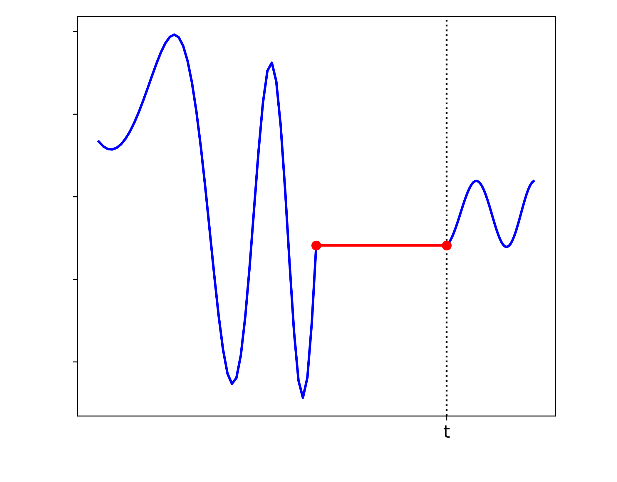
Continuous 1-dimensional path
$\mathbf{X}$

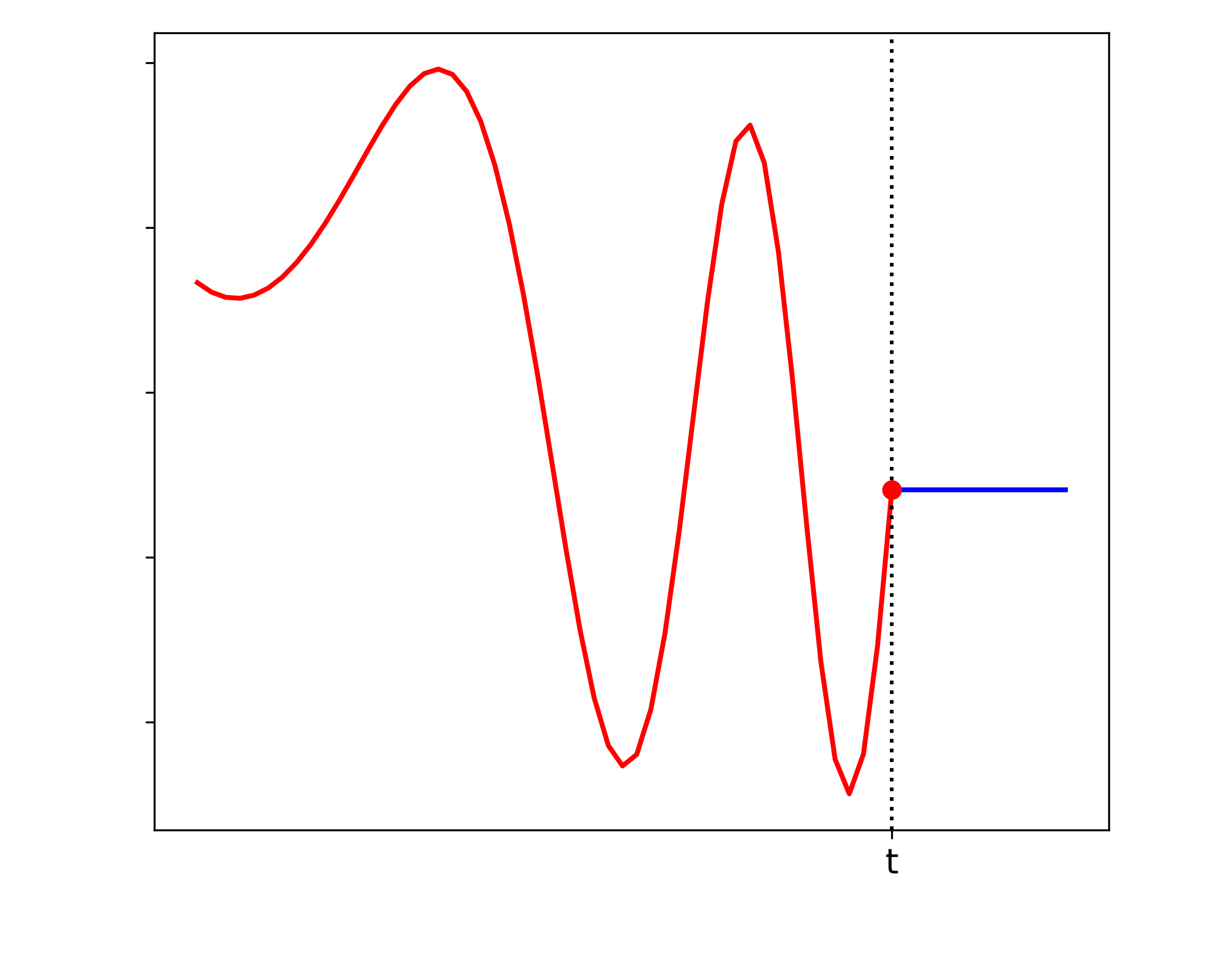
Stretched path on $[0,t]$
$\mathbf{X}^{t,\rhd}$

Remark 2.6.

1. Note that this time-stretching operation removes simply all constant parts of the path (except when $\mathbf{X}$ is constant on the whole interval $[0,t]$).

2. The definition of the time-stretched version path $\mathbf{X}^{t,\rhd}$ of a non-constant path on $[0,t]$ depends on the specific bijections $\theta^{k}$. Different bijections determine stretched versions that are time reparametrizations of one another, for some reparametrizations that map $[0,t]$ into $[0,t]$.

3. If one component of $\mathbf{X}$ is strictly increasing, for every $t\in(0,1]$ and $u\in[0,t)$, $\mathbf{X}^{t,\rhd}_{u}=\mathbf{X}_{u}$.

2.4 Marcus transformation of weakly geometric càdlàg rough paths

In this section, we recall the notion of the Marcus transformation of weakly geometric càdlàg $p$-rough paths for $p\in[1,3)$, introduced in Chevyrev (2017), (see also Section 2.3 in Chevyrev and Friz (2019)). This is an operation that associates every càdlàg path with continuous one obtained by introducing an additional time interval at each jump time and connecting the states before and after the jump via the so-called log-linear path-function denoted by $\ell\ell$. Let us start by listing all the objects required for the precise definition.

1. Fix $\mathbf{X}\in D([0,1],G^{[p]}(\mathbb{R}^{d}))$, and let $(t_{k})_{k\in\mathbb{N}}$ denote the sequence of its jumps times.

2. Fix a sequence $R:=(r_{k})_{k}$ such that for all $k\in\mathbb{N}$, $r_{k}>0$ and $\Sigma_{R}:=\sum_{k=1}^{\infty}r_{k}<\infty$, and define for all $t\in[0,1]$,

   $$\tau_{\mathbf{X},R}(t):=t+\sum_{k=1}^{\infty}r_{k}1_{\{t_{k}\leq t\}}.$$ (2.12)

   Notice that $\tau_{\mathbf{X},R}$ is an increasing càdlàg function from $[0,1]$ with values in $[0,1+\Sigma_{R}]$ whose sequence of jumps times coincide with the sequence of jumps times of $\mathbf{X}$.

3. Consider the log-linear path function $\ell\ell$ defined as follows:

   $$\ell\ell:G^{[p]}(\mathbb{R}^{d})\times G^{[p]}(\mathbb{R}^{d}) \rightarrow C([0,1],G^{[p]}(\mathbb{R}^{d}))$$

   $$(\mathbf{x},\mathbf{y}) \mapsto\Big{(}s\mapsto\mathbf{x}\otimes\exp^{([p])}(s\log^{({[p]})}(\mathbf{x}^{-1}\otimes\mathbf{y}))\Big{)}.$$ (2.13)

   Notice that for all $(\mathbf{x},\mathbf{y})\in G^{[p]}(\mathbb{R}^{d})\times G^{[p]}(\mathbb{R}^{d})$, $\ell\ell(\mathbf{x},\mathbf{y})(0)=\mathbf{x}$ and $\ell\ell(\mathbf{x},\mathbf{y})(1)=\mathbf{y}$.

4. Define $\mathbf{Y}\in C([0,1+\Sigma_{R}],G^{[p]}(\mathbb{R}^{d}))$ as follows: for all $s\in[0,1+\Sigma_{R}]$,

   $$\mathbf{Y}_{s}:=\begin{cases}\mathbf{X}_{t},&\text{if }s=\tau_{\mathbf{X},R}(t)\text{ for some }t\in[0,1];\\ \mathbf{X}_{t_{k}^{-}}\otimes\exp^{([p])}\left(\frac{(s-\tau_{\mathbf{X},R}(t_{k}^{-}))}{r_{k}}\log^{([p])}(\Delta\mathbf{X}_{t_{k}})\right)&\text{if }s\in[\tau_{\mathbf{X},R}(t_{k}^{-}),\tau_{\mathbf{X},R}(t_{k})],\ k\in\mathbb{N}.\end{cases}$$

Definition 2.7.

Let $\mathbf{X}\in D([0,1],G^{[p]}(\mathbb{R}^{d}))$. Fix a sequence $R$ as in (ii) and let $\tau_{\mathbf{X},R}$ be the increasing càdlàg function built through $R$ as in equation (2.12). Let $\mathbf{Y}$ be the continuous path defined via $\tau_{\mathbf{X},R}$ and the log-linear path function $\ell\ell$ as in (iv), and let $\psi_{R}$ denote an increasing bijection from $[0,1]$ to $[0,1+\Sigma_{R}]$. The Marcus-transformed path of $\mathbf{X}$ associated with the pair $(R,\psi_{R})$ is the continuous path $\widetilde{\mathbf{X}}\in C([0,1],G^{[p]}(\mathbb{R}^{d}))$ given by

$$\widetilde{\mathbf{X}}_{\cdot}:=\mathbf{Y}_{\psi_{R}(\cdot)}.$$

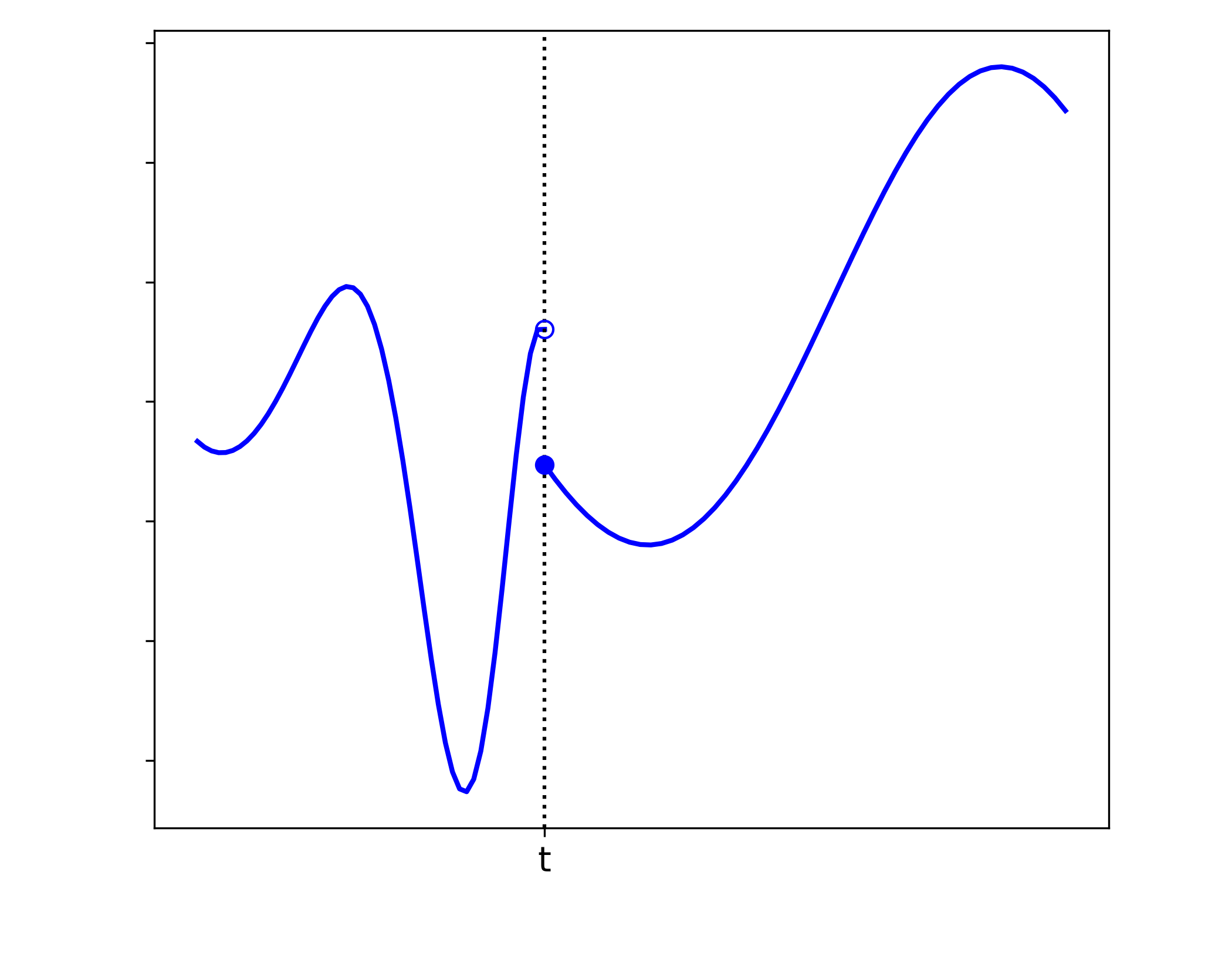
Càdlàg $1$-dimensional path
$\mathbf{X}$

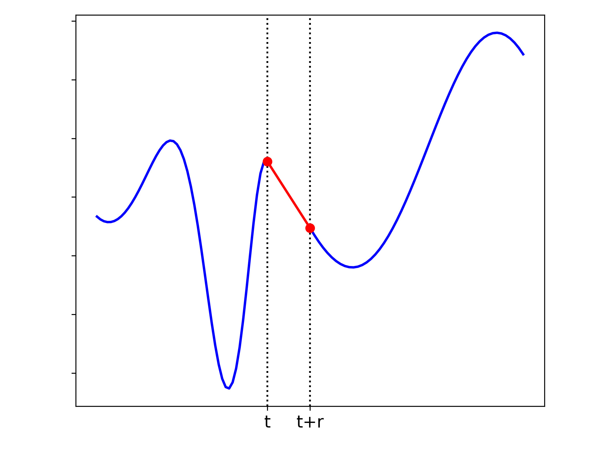
Marcus-transformed path
$\widetilde{\mathbf{X}}$

Assumption 2.8.

From now on, whenever we refer to the Marcus-transformed path of a càdlàg path $\mathbf{X}\in D([0,1],G^{[p]}(\mathbb{R}^{d}))$ associated to a pair $(R,\psi_{R})$, we implicitly assume that $R$ is a sequence satisfying condition (ii) and $\psi_{R}$ is an increasing bijection from $[0,1]$ to $[0,1+\Sigma_{R}]$.

Remark 2.9.

Fix $\mathbf{X}\in D([0,1],G^{[p]}(\mathbb{R}^{d}))$.

1. If $\mathbf{X}\in C([0,1],G^{[p]}(\mathbb{R}^{d})),$ for any sequence $R$ as in  (ii), the map $\tau_{\mathbf{X},R}$ in (2.12) is the identity map, i.e., $\tau_{\mathbf{X},R}(t)=t$ for all $t\in[0,1]$, and $\mathbf{Y}=\mathbf{X}$, for $\mathbf{Y}$ as in (iv). In this case, we establish the convention that $\psi_{R}$ is an increasing bijection from $[0,1]$ to $[0,1]$ and thus $\widetilde{\mathbf{X}}$ is simply a time-reparametrization of $\mathbf{X}$.

2. Let $\widetilde{\mathbf{X}}$ be the Marcus-transformed path of $\mathbf{X}$ associated to some pair $(R,\psi_{R})$. Observe that we can recover $\mathbf{X}$ from $\widetilde{\mathbf{X}}$ via

   $$\mathbf{X}_{\cdot}:=\widetilde{\mathbf{X}}_{\psi_{R}^{-1}(\tau_{\mathbf{X},R}(\cdot))}.$$

3. The Marcus-transformed paths of $\mathbf{X}$ associated with two different pairs $(R,\psi_{R})$ and $(\widetilde{R},\psi_{\widetilde{R}})$, are simply time-reparametrizations of one another. More precisely, let $\mathbf{Z}$ and $\widetilde{\mathbf{Z}}$ denote the transformed paths associated to $(R,\psi_{R})$ and $(\widetilde{R},\psi_{\widetilde{R}})$, respectively. Then ${\mathbf{Z}}_{\phi}=\widetilde{\mathbf{Z}}$ for some time-reparametrization $\phi$ such that for all $t\in[0,1]$,

   $$\phi(\psi_{R}^{-1}(\tau_{\mathbf{X},R}(t)))=\psi^{-1}_{\widetilde{R}}(\tau_{\mathbf{X},\widetilde{R}}(t)).$$

2.5 Signature of weakly geometric càdlàg rough paths

In this section, we recall the notion of the signature of weakly geometric càdlàg $p$-rough paths and the key idea behind its construction. More detailed discussions can be found in Friz and Atul (2017) and Chapter 1 in Primavera (2024).

The concept of the signature of a càdlàg rough path builds upon the established framework for continuous paths (see e.g., Lyons (1998)). More precisely, to compute the signature of a càdlàg rough path $\mathbf{X}\in D^{p}([0,1],G^{[p]}(\mathbb{R}^{d}))$ with $\mathbf{X}_{0}=\mathbf{1}$, the initial step involves transforming $\mathbf{X}$ into a continuous path via the Marcus transformation (with respect to some pair $(R,\psi_{R})$) detailed in Section 2.4. This transformation results in a path $\widetilde{\mathbf{X}}$ which is a continuous weakly geometric $p$-rough path by construction. Lyons’s extension theorem guarantees the existence (and uniqueness) of the signature of $\widetilde{\mathbf{X}}$ (see e.g., Theorem 9.5 in Friz and Victoir (2010)). The signature of the original càdlàg rough path $\mathbf{X}$ is defined then as the unique $G((\mathbb{R}^{d}))$-valued path $\mathbb{X}$ such that the projection paths over $G^{N}(\mathbb{R}^{d})$, denoted by $\mathbb{X}^{N}$, for $\mathbb{N}\ni N>[p]$, are the càdlàg paths given by

$$\mathbb{X}^{N}_{\cdot}:=\widetilde{\mathbb{X}}^{N}_{\psi_{R}^{-1}(\tau_{\mathbf{X},R}(\cdot))}.$$ (2.14)

Here $\widetilde{\mathbb{X}}^{N}$ denotes the extension path of $\widetilde{\mathbf{X}}$ provided by Theorem 9.5 in Friz and Victoir (2010) and $\tau_{\mathbf{X},R}$ the càdlàg map defined in equation (2.12).

These are the key ideas underlying the proof of the analogous theorem in the càdlàg context of Lyons’ extension theorem, on which the notion of signature relies.

Theorem 2.10.

(Minimal jump extension theorem, Theorem 20 in Friz and Atul (2017)) Let $\mathbb{N}\ni N>[p]$. Every $\mathbf{X}\in D^{p}([0,1],G^{[p]}(\mathbb{R}^{d}))$ with $\mathbf{X}_{0}=\mathbf{1}\in G^{[p]}(\mathbb{R}^{d}))$ admits a unique extension to a càdlàg path $\mathbb{X}^{N}:[0,1]\rightarrow G^{N}(\mathbb{R}^{d})$, such that $\mathbb{X}^{N}$ starts from $\mathbf{1}\in G^{N}(\mathbb{R}^{d})$, is of finite $p$-variation with respect to $d_{CC}$ on $G^{N}(\mathbb{R}^{d})$, and satisfies the following condition:

$$\log^{(N)}(\Delta\mathbb{X}_{t}^{N})=\log^{([p])}(\Delta\mathbf{X}_{t})\quad\text{for all }\ t\in[0,1].$$ (2.15)

Definition 2.11.

Let $\mathbf{X}\in D^{p}([0,1],G^{[p]}(\mathbb{R}^{d}))$ with $\mathbf{X}_{0}=\mathbf{1}\in G^{[p]}(\mathbb{R}^{d}))$. The signature of $\mathbf{X}$ is defined as the unique path

$$\mathbb{X}:[0,1]\rightarrow G((\mathbb{R}^{d})),$$

such that for all $\mathbb{N}\ni N>[p]$, $\pi_{\leq N}(\mathbb{X})=\mathbb{X}^{N}$, where $\mathbb{X}^{N}$ denotes the unique extension path of $\mathbf{X}$ in $G^{N}(\mathbb{R}^{d})$ provided by Theorem 2.10.

Notation 2.12.

From now on, given $\mathbf{X}\in D^{p}([0,1],G^{[p]}(\mathbb{R}^{d}))$, we refer to $\mathbb{X}$ as signature of $\mathbf{X}$ and to $\mathbb{X}^{N}$ as truncated signature of order $N$ of $\mathbf{X}$.

Finally, the truncated signature of a weakly geometric càdlàg rough path can be computed by solving a (Marcus-type) RDE (see Chevyrev and Friz (2019)).

Corollary 2.13 (Corollary 39 in Friz and Atul (2017)).

Let $\mathbf{X}\in D^{p}([0,1],G^{[p]}(\mathbb{R}^{d}))$ with $\mathbf{X}_{0}=\mathbf{1}\in G^{[p]}(\mathbb{R}^{d}))$ and $\mathbb{N}\ni N>[p]$. The unique extension path $\mathbb{X}^{N}$ of $\mathbf{X}$ with values in $G^{N}(\mathbb{R}^{d})$ provided by Theorem 2.10 satisfies the following linear Marcus-type RDE

$$d\mathbb{X}^{N}=\mathbb{X}^{N}\otimes\diamond d\mathbf{X},\qquad\mathbb{X}^{N}_{0}=\mathbf{1}\in G^{N}(\mathbb{R}^{d}),$$ (2.16)

which admits a unique solution, whose explicit form can be written as

$$\mathbb{X}^{N}_{\cdot}=1+\int_{0}^{\cdot}\mathbb{X}^{N}_{s^{-}}\otimes d\mathbf{X}_{s}+\sum_{0<s\leq\cdot}\mathbb{X}^{N}_{s^{-}}\otimes\big{(}\exp^{(N)}(\log^{([p])}(\Delta\mathbf{X}_{s}))-\Delta\mathbf{X}_{s}\big{)}.$$ (2.17)

The integral in (2.17) is understood as a Young (if $p\in[1,2)$) or level 2 rough (if $p\in[2,3)$) integral (see Section E.1) and the summation term is well-defined as an absolutely summable series.

Fix $\mathbf{u}\in T(\mathbb{R}^{d})$ and recall the shifts introduced in equation (2.7). Let $\mathbf{X}\in D^{p}([0,1],G^{[p]}(\mathbb{R}^{d}))$ with $\mathbf{X}_{0}=\mathbf{1}$ and denote by $\mathbb{X}$ its signature. Then, a projection of equation (2.17) along $\mathbf{u}$ combined with Lemma 2.9 in Friz and Zhang (2017) yields that

1. if $p\in[1,2)$,

   $$\langle\mathbf{u},\mathbb{X}_{\cdot}\rangle= \langle\mathbf{u},\mathbb{X}_{0}\rangle+\int_{0}^{\cdot}\langle\mathbf{u}^{(1)},\mathbb{X}_{s^{-}}\rangle d\mathbf{X}_{s}$$ (2.18)

   $$+\sum_{0<s\leq\cdot}\langle\mathbf{u},\mathbb{X}_{s}\rangle-\langle\mathbf{u},\mathbb{X}_{s^{-}}\rangle-\langle\mathbf{u}^{(1)},\mathbb{X}_{s^{-}}\rangle\Delta X_{s},$$

   where the integral is a Young integral of $\langle\mathbf{u}^{(1)},\mathbb{X}_{\cdot}\rangle\in D^{p}([0,1],\mathbb{R}^{d+1})$ with respect to $\mathbf{X}$, and for all $t\in(0,1]$, we set $(1,\Delta X_{t}):=\Delta\mathbf{X}_{t}$.

2. if $p\in[2,3)$,

   $$\langle\mathbf{u},\mathbb{X}_{\cdot}\rangle= \langle\mathbf{u},\mathbb{X}_{0}\rangle+\int_{0}^{\cdot}\langle\mathbf{u}^{(1)},\mathbb{X}_{s^{-}}\rangle d\mathbf{X}_{s}$$ (2.19)

   $$+\sum_{0<s\leq\cdot}\langle\mathbf{u},\mathbb{X}_{s}\rangle-\langle\mathbf{u},\mathbb{X}_{s^{-}}\rangle-\langle\mathbf{u}^{(1)},\mathbb{X}_{s^{-}}\rangle\Delta X_{s}-\langle\mathbf{u}^{(2)},\mathbb{X}_{s^{-}}\rangle\Delta\mathbb{X}^{(2)}_{s},$$

   where the integral is a (level 2) rough integral of the controlled rough path $\big{(}\langle\mathbf{u}^{(1)},\mathbb{X}_{\cdot}\rangle,\langle\mathbf{u}^{(2)},\mathbb{X}_{\cdot}\rangle\big{)}\in\mathcal{V}^{p,\frac{p}{2}}_{\mathbf{X}}$ (Definition 2.3) with respect to $\mathbf{X}$, and for all $t\in(0,1]$, we set $(1,\Delta X_{t},\Delta\mathbb{X}^{(2)}_{t}):=\Delta\mathbf{X}_{t}$.

Assumption 2.14.

Throughout, we assume that all the weakly geometric càdlàg rough paths start at $\mathbf{1}\in G^{[p]}(\mathbb{R}^{d})$, i.e., $\mathbf{X}_{0}=\mathbf{1}$.

3 Functionals of weakly geometric càdlàg rough paths

3.1 Non-anticipative Marcus canonical path functionals

Inspired by the notion of Marcus-type-RDEs (see Chevyrev and Friz (2019)), we here introduce the class of so-called non-anticipative Marcus canonical path functionals. To this end, we start with the notion of non-anticipative path functionals, which in turn relies on the definition of stopped-paths. In the following, we set $\mathbb{N}_{0}:=\mathbb{N}\cup\{0\}.$

Definition 3.1.

Given ${{\mathbf{X}}}\in{D}^{p}([0,1],G^{[p]}(\mathbb{R}^{d})))$ and $t\in[0,1]$, we define the stopped weakly geometric càdlàg rough path of ${\mathbf{X}}$ stopped at time $t$ as the càdlàg path ${\mathbf{X}}^{t}:[0,1]\rightarrow G^{[p]}(\mathbb{R}^{d})$ given by

$${\mathbf{X}}^{t}_{u}:={\mathbf{X}}_{u}1_{\{u<t\}}+{\mathbf{X}}_{t}1_{\{u\geq t\}},$$

for all $u\in[0,1]$.

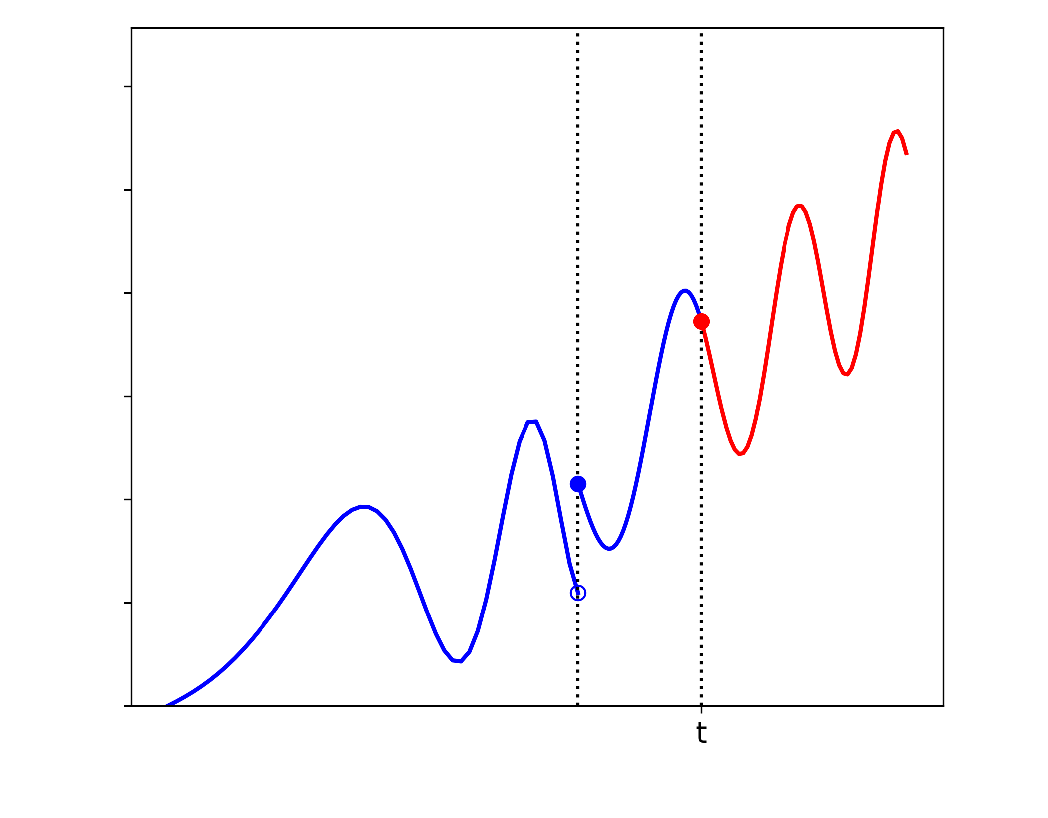
Càdlàg $1$-dimensional path
$\mathbf{X}$

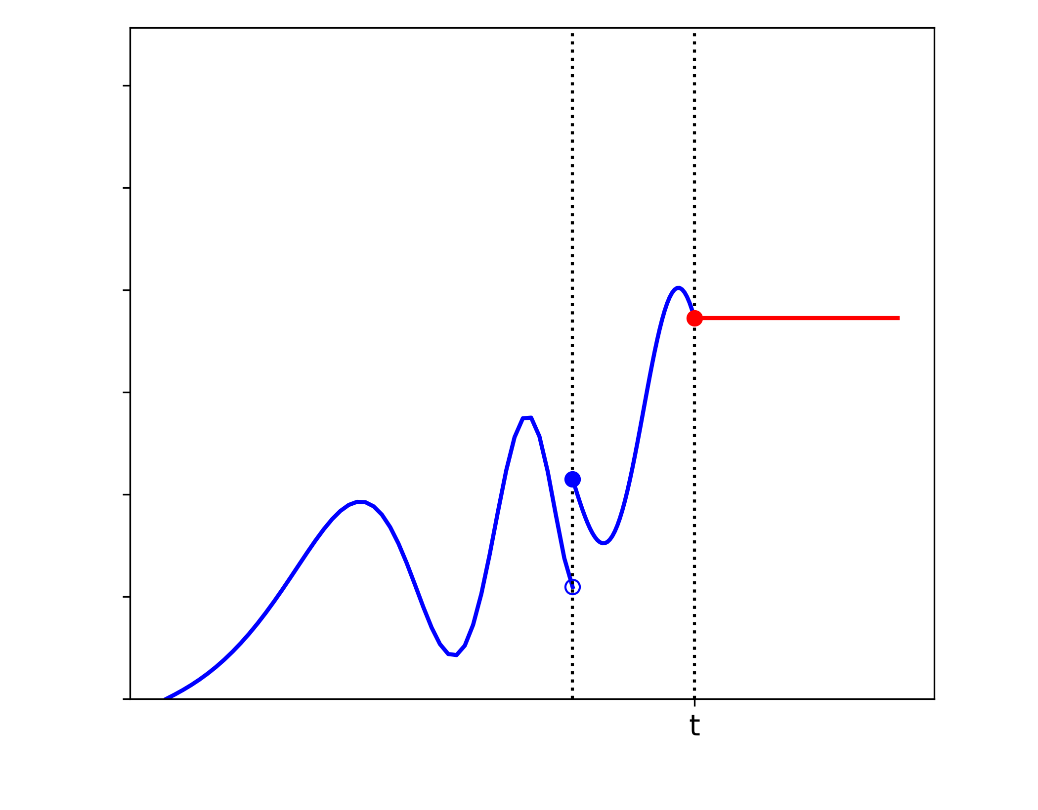
Càdlàg path stopped at time $t$
$\mathbf{X}^{t}$

Definition 3.2.

Let $F:[0,1]\times D([0,1],G^{[p]}(\mathbb{R}^{d}))\rightarrow\mathbb{R}$. We say that $F$ is a non-anticipative path functional if for all $(t,\mathbf{X})\in[0,1]\times D([0,1],G^{[p]}(\mathbb{R}^{d}))$, it holds that

$$F(t,\mathbf{X})=F(t,\mathbf{X}^{t}).$$

Remark 3.3.

The variable $t$ has the role of a parameter and not of a component of the path $\mathbf{X}$. In fact, it is the parameter needed to specify that the path functional is non-anticipative.

Let us now introduce the class of the non-anticipative Marcus canonical path functionals. We refer to Chevyrev and Friz (2019) and also  Fujiwara and Kunita (1985), Applebaum and Tang (2001), Kurtz et al. (1995) for some related definitions from the literature.

For $\mathbf{X}\in D([0,1],G^{[p]}(\mathbb{R}^{d}))$, recall the notion of a Marcus-transformed path of $\mathbf{X}$ associated with some pair $(R,\psi_{R})$ given in Definition 2.7 and the one of time-stretched path given in Definition 2.5.

Definition 3.4.

Let $F:[0,1]\times D([0,1],G^{[p]}(\mathbb{R}^{d}))\rightarrow\mathbb{R}$ be a non-anticipative path functional. We say that $F$ is a non-anticipative Marcus canonical path functional if

1. for all $\mathbf{X}\in C([0,1],G^{[p]}(\mathbb{R}^{d}))$, $t\in[0,1]$, $\phi$ time-reparametrization,

   $$F(t,\mathbf{X}_{\phi})=F(\phi(t),\mathbf{X});$$

2. for all $\mathbf{X}\in C([0,1],G^{[p]}(\mathbb{R}^{d}))$ and all $t\in[0,1]$,

   $$F(t,\mathbf{X})=F(t,\mathbf{X}^{t,\rhd}),$$

   where $\mathbf{X}^{t,\rhd}$ denotes some time-stretched version of $\mathbf{X}$ on $[0,t]$;

3. for all $(t,\mathbf{X})\in[0,1]\times D([0,1],G^{[p]}(\mathbb{R}^{d})),$

   $$F(t,\mathbf{X})=F(\psi_{R}^{-1}(\tau_{\mathbf{X},R}(t)),\widetilde{\mathbf{X}}),$$

   where $\widetilde{\mathbf{X}}$ denotes the Marcus-transformed path of $\mathbf{X}$ with respect to some pair $(R,\psi_{R})$.

We denote the space of such functionals by $\mathcal{M}_{[p]}^{0}$.

Notation 3.5.

We set $((\mathcal{M}_{[p]}^{0})^{d})^{\otimes 0}:=\mathcal{M}_{[p]}^{0}$ and for $m\in\mathbb{N}_{0}$, we write $F\in((\mathcal{M}_{[p]}^{0})^{d})^{\otimes m}$ if

$$F:[0,1]\times D([0,1],G^{[p]}(\mathbb{R}^{d}))\rightarrow(\mathbb{R}^{d})^{\otimes m}$$

is a path functional whose components are non-anticipative Marcus canonical path functionals in the sense of Definition 3.4.

Remark 3.6.

1. The symbol $\mathcal{M}_{[p]}^{0}$ does not include the dimension $d$, as it will always be clear from the context.

2. Property (i) in Definition 3.4 guarantees that the subsequent conditions (ii), (iii) are independent of the specific stretched version of $\mathbf{X}$ on $[0,t]$ and independent of the specific Marcus-transformed path, respectively. Indeed, let ${\mathbf{Z}}$, ${\widetilde{\mathbf{Z}}}$ be two Marcus transformations of $\mathbf{X}$ associated with $(R,\psi_{R})$ and $(\widetilde{R},\psi_{\widetilde{R}})$, respectively. By Remark 2.9 (iii), ${\mathbf{Z}}_{\phi}=\widetilde{\mathbf{Z}}$, for some time-reparametrization $\phi$, and for all $t\in[0,1]$,

   $$\phi(\psi^{-1}_{\widetilde{R}}(\tau_{\mathbf{X},\widetilde{R}}(t)))=\psi_{R}^{-1}(\tau_{\mathbf{X},R}(t)).$$

   Therefore, by condition (i),

   $$F(\psi^{-1}_{\widetilde{R}}(\tau_{\mathbf{X},\widetilde{R}}(t)),\widetilde{\mathbf{Z}})=F(\psi^{-1}_{{R}}(\tau_{\mathbf{X},{R}}(t)),\mathbf{Z}).$$ (3.1)

   Recalling Remark 2.6(ii), a similar argument holds for condition (ii).

3. A non-anticipative path functional defined only on the set of continuous paths that satisfies conditions (i),(ii) of Definition 3.4 can always be extended to a path functional on the entire set of càdlàg path via condition (iii) of Definition 3.4. The resulting functional is a well-defined Marcus canonical path functional. Moreover, this extension is also unique. This is in fact the approach proposed in Chevyrev and Friz (2019).

Notation 3.7.

Given the independence on the specific Marcus-transformed path discussed in Remark 3.6 and to ease notation, for all $t\in[0,1]$, $\mathbf{X}\in D([0,1],G^{[p]}(\mathbb{R}^{d}))$ and a pair $(R,\psi_{R})$, we set $\mu_{t}:=\psi_{R}^{-1}(\tau_{\mathbf{X},R}(t))$ whenever there is no ambiguity.

We present some examples of non-anticipative Marcus canonical path functionals.

Example 3.8.

1. Let $F(t,\mathbf{X}):=Y_{t}$, where $Y$ denotes the solution of a Marcus-type RDE in the sense of Definition 3.1 in Chevyrev and Friz (2019), driven by some càdlàg path $\mathbf{X}\in D^{p}([0,1],G^{[p]}(\mathbb{R}^{d}))$, at time $t\in(0,1]$. By the solution concept and the property of the rough integral, $F$ is a non-anticipative Marcus canonical path functional.

2. Let $F$ be the functional such that for all $(t,\mathbf{X})\in[0,T]\times D^{p}([0,1],G^{[p]}(\mathbb{R}^{d}))$,

   $$F(t,\mathbf{X}):=\sup_{s\in[0,t]}\|\mathbf{X}_{s}\|.$$

   Then F is a non-anticipative Marcus canonical path functional.

3. For $\mathbf{X}\in C^{1}([0,1],G^{1}(\mathbb{R}^{2}))$, set $\mathbf{X}^{1}_{\cdot}:=\langle\epsilon_{1},\mathbf{X}_{\cdot}\rangle=$ and $\mathbf{X}^{2}_{\cdot}:=\langle\epsilon_{2},\mathbf{X}_{\cdot}\rangle$, and consider the path functional (defined only on the set of continuous paths) via $F(t,\mathbf{X}):=\int_{0}^{t}\mathbf{X}^{1}_{s}d\mathbf{X}^{2}_{s}$. Since $F$ verifies (i),(ii) of Definition 3.4, following the discussion in Remark 3.6(iii), we can extend it to the set $D^{1}([0,1],G^{1}(\mathbb{R}^{2}))$ via condition (iii). A direct computation shows that the resulting functional, which is non-anticipative Marcus canonical and we still denote by $F$, explicitly reads as

   $$F(t,\mathbf{X}):=\int_{0}^{t}\mathbf{X}^{1}_{s^{-}}d\mathbf{X}^{2}_{s}+\frac{1}{2}\sum_{0<s\leq t}\Delta\mathbf{X}^{1}_{s}\Delta\mathbf{X}^{2}_{s},$$ (3.2)

   for all $(t,\mathbf{X})\in D^{1}([0,1],G^{1}(\mathbb{R}^{2}))$.

Remark 3.9.

1. It is important to note that not every non-anticipative path functional that is well defined on the space of càdlàg paths is a Marcus canonical path functional. Consider for instance the functional defined via $F(t,\mathbf{X}):=\int_{0}^{t}\mathbf{X}^{1}_{s^{-}}d\mathbf{X}^{2}_{s}$, for all $(t,\mathbf{X})\in D^{1}([0,1],G^{1}(\mathbb{R}^{2}))$. Then, $F$ is not Marcus canonical . Indeed, for $\mathbf{X}\in D^{1}([0,1],G^{1}(\mathbb{R}^{2}))\setminus C^{1}([0,1],G^{1}(\mathbb{R}^{2}))$, let $\widetilde{\mathbf{X}}$ be its Marcus-transformed path with respect to some pair $(R,\psi_{R})$. Then,

   $$F(\psi_{R}^{-1}(\tau_{\mathbf{X},R}(t)),\widetilde{\mathbf{X}})=\int_{0}^{t}\mathbf{X}^{1}_{s^{-}}d\mathbf{X}^{2}_{s}+\frac{1}{2}\sum_{0<s\leq t}\Delta\mathbf{X}^{1}_{s}\Delta\mathbf{X}^{2}_{s}\neq F(t,\mathbf{X}).$$

   Similarly, the path functional given by $F(t,\mathbf{X}):=\sum_{0<s\leq t}\Delta\mathbf{X}^{1}_{s}\Delta\mathbf{X}^{2}_{s}$ is not Marcus canonical as $0=F(\psi_{R}^{-1}(\tau_{\mathbf{X},R}(t)),\widetilde{\mathbf{X}})\neq F(t,\mathbf{X})$ for pure jump paths.

2. Note however that some non-anticipative path functionals that do not appear to be Marcus canonical at first glance can be easily turned into Marcus canonical ones. This is the case for instance for the functional $F$ defined via $F(t,\mathbf{X}):=\int_{0}^{t}\mathbf{X}_{s}ds$ for all $(t,\mathbf{X})\in[0,1]\times C^{1}([0,1],G^{1}(\mathbb{R}))$, which does not satisfy condition (i) in Definition 3.4. However, considering the path functional $\bar{F}(t,\mathbf{X}):=\int_{0}^{t}\mathbf{X}^{2}_{s}d\mathbf{X}_{s}^{1}$ defined on $[0,1]\times C^{1}([0,1],G^{1}(\mathbb{R}^{2}))$, we get that it satisfies property (i) in Definition 3.4, and for all $(t,\widehat{\mathbf{X}})\in[0,1]\times C^{1}([0,1],G^{1}(\mathbb{R}^{2}))$ where $\widehat{\mathbf{X}}:=(Id,\mathbf{X})$, with $Id_{u}:=u$ for all $u\in[0,1]$ and $\mathbf{X}\in C^{1}([0,1],G^{1}(\mathbb{R}))$, it holds that $F(t,\mathbf{X})=\bar{F}(t,\widehat{\mathbf{X}})$. Therefore, a time-extension of the original path can be crucial to satisfy the conditions specified in Definition 3.4.

   The above example also illustrates that a functional may have multiple representations. To apply the theory that follows, it is necessary to select the representation that satisfies the conditions for being a non-anticipative Marcus canonical path functional.

Next, we introduce the notion of path functionals that are invariant under reparametrization, which is the same as condition (i) in Definition 3.4, however on the whole space of càdlàg paths $D([0,1],G^{[p]}(\mathbb{R}^{d}))$ and not only on $C([0,1],G^{[p]}(\mathbb{R}^{d}))$.

Definition 3.10.

Let $F:[0,1]\times D([0,1],G^{[p]}(\mathbb{R}^{d}))\rightarrow\mathbb{R}$ be a non-anticipative path functional. We say that $F$ is invariant under reparametrization if for all $\mathbf{X}\in D([0,1],G^{[p]}(\mathbb{R}^{d}))$, $t\in[0,1]$ and $\phi$ time-reparametrization,

$$F(t,\mathbf{X}_{\phi})=F(\phi(t),\mathbf{X}).$$

We now show that every $F\in\mathcal{M}^{0}_{[p]}$ satisfies this property. The proof of the following proposition is given in Appendix A.1.

Proposition 3.11.

Let $F\in\mathcal{M}^{0}_{[p]}$. Then $F$ is invariant under reparametrization.

To conclude, we introduce the notion of the remainder path functional related to some functionals of $G^{2}(\mathbb{R}^{d})$-valued paths.

Definition 3.12.

Let $F\in((\mathcal{M}_{[p]}^{0})^{d})^{\otimes m}$ and $F^{\prime}\in((\mathcal{M}_{[p]}^{0})^{d})^{\otimes m+1}$, for $m\in\mathbb{N}_{0}$. We define the remainder path functional (related to $F$ and $F^{\prime}$) as follows:

$$R^{F,F^{\prime}}:\Delta_{1}\times D([0,1],G^{2}(\mathbb{R}^{d}))\rightarrow(\mathbb{R}^{d})^{\otimes m},$$

given by

$$R^{F,F^{\prime}}((s,t),\mathbf{X}):=F(t,\mathbf{X})-F(s,\mathbf{X})-F^{\prime}(s,\mathbf{X})\pi_{1}(\mathbf{X}_{s,t}),$$

for all $((s,t),\mathbf{X})\in\Delta_{1}\times D([0,1],G^{2}(\mathbb{R}^{d}))$.

3.2 Vertically differentiable path functionals

Definition 3.13.

Let $F\in\mathcal{M}^{0}_{[p]}$. We say that $F$ is vertically differentiable at $(t,\mathbf{X})\in[0,1]\times D([0,1],G^{[p]}(\mathbb{R}^{d}))$ in the direction $i=1,\dots,d$ if the map

$$\mathbb{R}\ni h\mapsto F(\mu_{t},\widetilde{\mathbf{X}}\otimes\exp^{([p])}(h\epsilon_{i})1_{\{\cdot\geq\mu_{t}\}})$$

is differentiable at $0$, for some Marcus-transformed path $\widetilde{\mathbf{X}}$ and $\mu_{t}\in[0,1]$ given in Notation 3.7. In this case we call

$$\frac{d}{dh}F(\mu_{t},\widetilde{\mathbf{X}}\otimes\exp^{([p])}(h\epsilon_{i})1_{\{\cdot\geq\mu_{t}\}})|_{h=0}.$$ (3.3)

the vertical derivative of $F$ at $(t,\mathbf{X})$ in the direction $i$. If $F$ is vertically differentiable in all directions $i=1,\dots,d$ at all $(t,\mathbf{X})$, we say that $F$ is vertically differentiable. We denote the space of such functionals by $\mathcal{M}_{[p]}^{1}$.

Remark 3.14.

1. The value of the vertical derivatives of $F\in\mathcal{M}_{[p]}^{1}$ at some $(t,\mathbf{X})$ is independent of the specific Marcus-transformed path. This follows from Proposition 3.11 and a similar reasoning as in Remark 3.6.

2. In (3.3) the Marcus transformation of the path is computed before the vertical perturbation. This is, in fact, a key aspect of this definition. On one hand, it allows the preservation of the Marcus property of the functionals also at the level of the (functional) derivative (see Proposition 3.15). On the other hand, if the original path $\mathbf{X}$ admits a jump a time $t$, the Marcus property of the functional $F$ allows to interpret the derivative in (3.3) as a derivative computed via a delayed perturbation of the original path:

   $$\mathbf{X}^{t}+h\epsilon_{i}1_{\{\cdot\geq t+\varepsilon\}},$$ (3.4)

   for some $\varepsilon>0$ independent on the specific pair employed for computing $\widetilde{\mathbf{X}}$.

   To clarify this aspect, suppose that $\mathbf{X}$ is a weakly geometric càdlàg $p$-rough path, for $p\in[1,2)$, that admits a jump only at time $t$. For simplicity, we identify $G^{1}(\mathbb{R}^{d})$ with $\mathbb{R}^{d}$. Then, applying the Marcus transformation first to the path $\mathbf{X}$ and then to the perturbed path $\widetilde{\mathbf{X}}+h\epsilon_{i}1_{\{\cdot\geq\mu_{t}\}}$ yields that (3.3) explicitly reads as

   $$\frac{d}{dh}F(t+\delta_{2}+\delta_{1},\mathbf{Y}^{[i]}(h))|_{h=0},$$

   for $\mathbf{Y}^{[i]}(h)$ defined up to time $t+\delta_{2}+\delta_{1}$ via

   $$\mathbf{Y}^{[i]}(h)_{s}:=\begin{cases}\mathbf{X}_{s^{-}}&\text{if }s\in[0,t],\\ \mathbf{X}_{t^{-}}+\frac{s-t}{\delta_{2}}\Delta\mathbf{X}_{t}&\text{if }s\in[t,t+\delta_{2}],\\ \mathbf{X}_{t^{-}}+\Delta\mathbf{X}_{t}+\frac{s-t-\delta_{2}}{\delta_{1}}h\epsilon_{i}&\text{if }s\in[t+\delta_{2},t+\delta_{2}+\delta_{1}],\end{cases}$$

   for some $\delta_{2},\delta_{1}>0$ such that $t+\delta_{2}+\delta_{1}<1$, $\mu_{t}=t+\delta_{2}$. Since the path $\mathbf{Y}^{[i]}(h)$ stopped at time $t+\delta_{2}+\delta_{1}$ is a time-stretched version of some Marcus-transformed path of (3.4) on $[0,\mu_{t+\varepsilon}]$, for $\mu_{t+\varepsilon}=t+\delta_{2}+\delta_{1}$, by conditions (ii) and (iii), we get

   $$\frac{d}{dh}F(t+\varepsilon,\mathbf{X}^{t}+h\epsilon_{i}1_{\{\cdot\geq t+\varepsilon\}})|_{h=0}=\frac{d}{dh}F(t+\delta_{2}+\delta_{1},\mathbf{Y}^{[i]}(h))|_{h=0}.$$

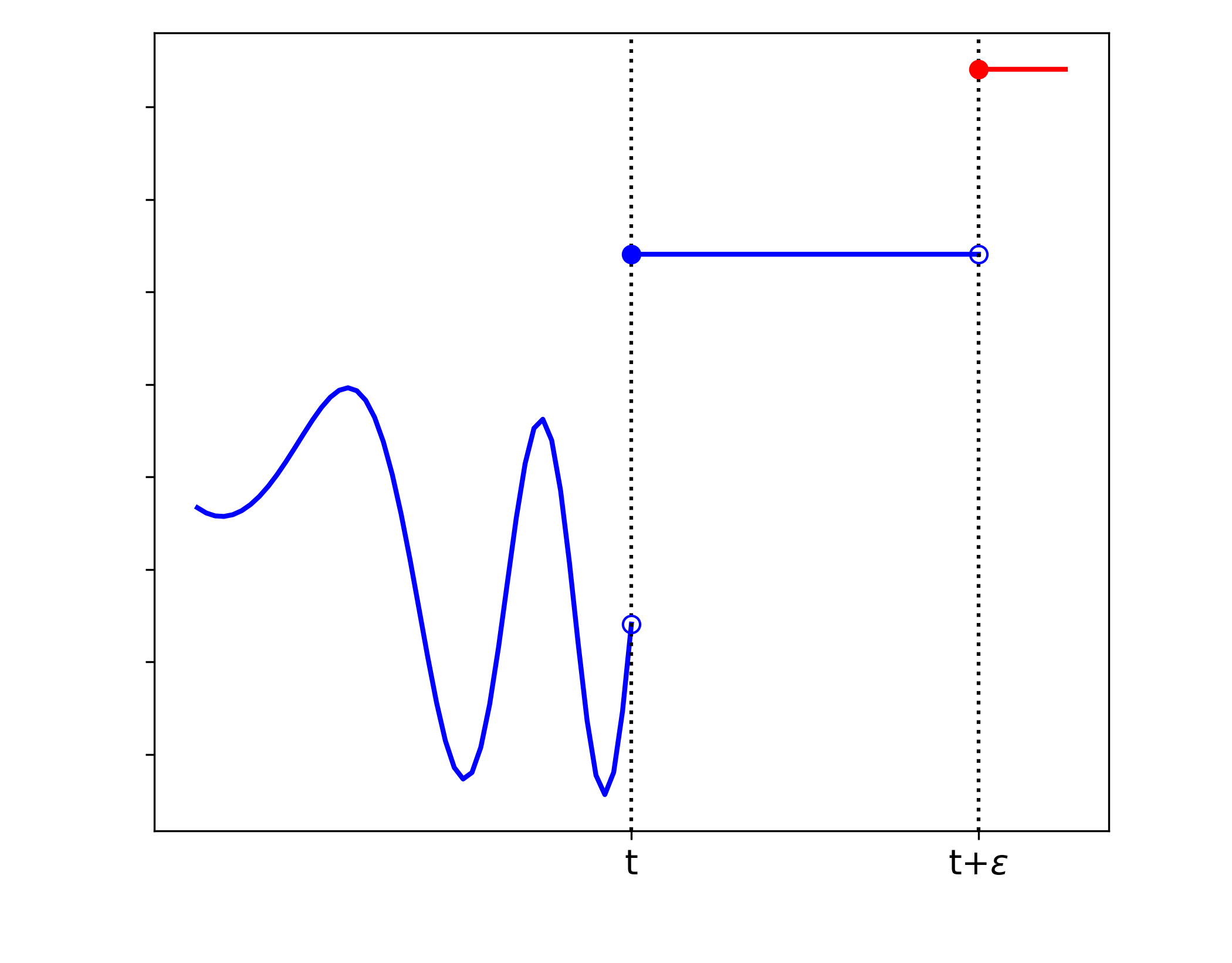
   Delayed vertical perturbation
   $\mathbf{X}^{t}+h\epsilon_{1}1_{\{\cdot\geq t+\varepsilon\}}$

   

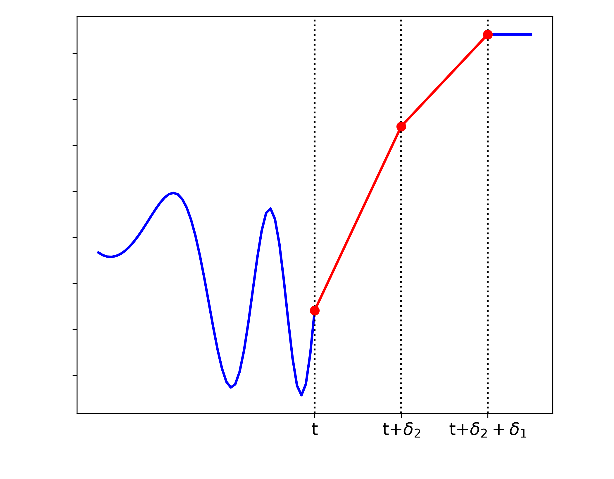
   Stretched Marcus tranformation
   $\mathbf{Y}^{[1]}(h)$

   

   This confirms that our notion of vertical derivative involving Marcus transformations of the original path allows to view the derivative in (3.3) as a derivative computed via a delayed perturbation of the original path. This aspect affects in particular the higher order vertical derivatives where a jump at the current time always occurs (see Remark 3.20 and Example 3.19). Notice furthermore that the independence on the specific $\varepsilon>0$ follows by the invariance of the functional with respect to time-reparametrization.

3. If $p\in[1,2)$, the notion of vertical derivatives given in Definition 3.13 corresponds to the notion of vertical derivatives introduced in Dupire (2009) (see also Definition 8 in Cont and Fournie (2010a)) when evaluated at continuous paths.

   Similarly, if for $p\in[2,3)$ a non-anticipative path functional depends only on $\pi_{1}(\mathbf{X})$ for all $(t,\mathbf{X})$, then (3.3) matches again the notion of vertical derivative introduced in Dupire (2009) evaluated at continuous paths.

Next, we introduce the notion of higher-order vertical derivatives, which are given via an iterative application of the computation in (3.3). To make the argument precise, we formally introduce the differential that associates to every path functional its derivative functional. The well-posedness of this concept relies on the following proposition, whose proof is given in Appendix A.2.

Proposition 3.15.

Let $F\in\mathcal{M}^{1}_{[p]}$. The path functional given by

$$[0,1] \times D([0,1],G^{[p]}(\mathbb{R}^{d}))\rightarrow\mathbb{R}$$ (3.5)

$$(t,\mathbf{X})\longmapsto\frac{d}{dh}F(\mu_{t},\widetilde{\mathbf{X}}\otimes\exp^{([p])}(h\epsilon_{i})1_{\{\cdot\geq\mu_{t}\}})|_{h=0},$$

is a non-anticipative Marcus canonical path functional.

Definition 3.16.

For all $i=1,\dots,d$, we define the differential operators

$$U^{i}:\ \mathcal{M}^{1}_{[p]}\rightarrow\mathcal{M}^{0}_{[p]}$$

$$\ F\mapsto U^{i}(F),$$

where for all $F\in\mathcal{M}^{1}_{[p]}$ and all $(t,\mathbf{X})\in[0,1]\times D([0,1],G^{[p]}(\mathbb{R}^{d}))$,

$$U^{i}(F)(t,\mathbf{X}):=\frac{d}{dh}F(\mu_{t},\widetilde{\mathbf{X}}\otimes\exp^{([p])}(h\epsilon_{i})1_{\{\cdot\geq\mu_{t}\}})|_{h=0},$$

for some Marcus-transformed path $\widetilde{\mathbf{X}}$ and $\mu_{t}\in[0,1]$ given in Notation 3.7.

Finally, we introduce the notion of higher-order vertical derivatives.

Definition 3.17.

Let $F\in\mathcal{M}^{0}_{[p]}$ and $K\in\mathbb{N}$. We say that $F$ is $K$ times vertically differentiable if for all $l=1,\dots,K$ the path functionals defined recursively by

$$U^{i_{0}}F:=F,\qquad\qquad\qquad\qquad\qquad\qquad\quad\qquad\quad\text{for }l=1,$$

$$U^{i_{l-1}}\dots U^{i_{1}}U^{i_{0}}F:=U^{i_{l-1}}(U^{i_{l-2}}\dots U^{i_{1}}U^{i_{0}}F),\quad\text{for }l=2,\dots,K,\ (i_{1},\dots,i_{l-1})\in\{1,\dots,d\}^{l-1},$$

are vertically differentiable at all $(t,\mathbf{X})\in[0,1]\times D([0,1],G^{[p]}(\mathbb{R}^{d}))$. In this case, we call

$$U^{i_{K}}\dots U^{i_{1}}F(t,\mathbf{X}):=U^{i_{K}}(U^{i_{K-1}}\dots U^{i_{1}}U^{i_{0}}F)(t,\mathbf{X})$$ (3.6)

the vertical derivative of order $K$ of $F$ at $(t,\mathbf{X})$ in the directions $(i_{1},\dots,i_{K})\in\{1,\dots,d\}^{K}$. We denote the space of such functionals by $\mathcal{M}_{[p]}^{K}$.

Notation 3.18.

In the following, for $K\in\mathbb{N}$, $F\in\mathcal{M}_{[p]}^{K}$, $l=1,\dots,K$, we let $\nabla^{l}F$ denote the $(\mathbb{R}^{d})^{\otimes l}$-valued path functional such that for all $I=(i_{1},\dots,i_{l})$,

$$\nabla^{l}F(t,\mathbf{X})_{I}:=U^{i_{l}}\dots U^{i_{1}}F(t,\mathbf{X}),$$

for all $(t,\mathbf{X})\in[0,1]\times D([0,1],G^{[p]}(\mathbb{R}^{d}))$. Notice that $\nabla^{l}F$ is a $(\mathbb{R}^{d})^{\otimes l}$-valued path functional whose components are in $\mathcal{M}_{[p]}^{K-l}$. For notational convenience, we also write $\nabla^{0}F:=F$ and $\nabla F:=\nabla^{1}F$.

The computation of the higher-order vertical derivatives can be done by considering the iterative procedure described below. For notational simplicity, we here consider only càdlàg paths with values in $G^{1}(\mathbb{R}^{d})$, identify $G^{1}(\mathbb{R}^{d})$ as $\mathbb{R}^{d}$, and explicitly write the procedure for computing the derivatives up to the second order.

Let $F:[0,1]\times D([0,1],G^{1}(\mathbb{R}^{d}))\rightarrow\mathbb{R}$ and assume $F\in\mathcal{M}^{2}_{1}$. Fix $\mathbf{X}\in D([0,1],G^{1}(\mathbb{R}^{d}))$, $t\in[0,1]$.

$$\begin{array}[]{l l}\text{Step 0:}&\mathbf{X}^{[0]}:=\mathbf{X}^{t},\\ &\mathbf{Y}^{[0]}:=\ThisStyle{\stackengine{.8\LMpt}{\SavedStyle\mathbf{X}^{[0]}}{\stretchto{\scaleto{\SavedStyle\mkern 0.2mu\sim}{.5467}}{.5}}{O}{c}{F}{T}{S}},\\ &\mu_{t}^{[0]}:=\psi_{R_{0}}^{-1}(\tau_{\mathbf{X}^{[0]},R_{0}}(t)),\text{ for some pair }(R_{0},\psi_{R_{0}}).\end{array}$$

Figure 1: Step 0

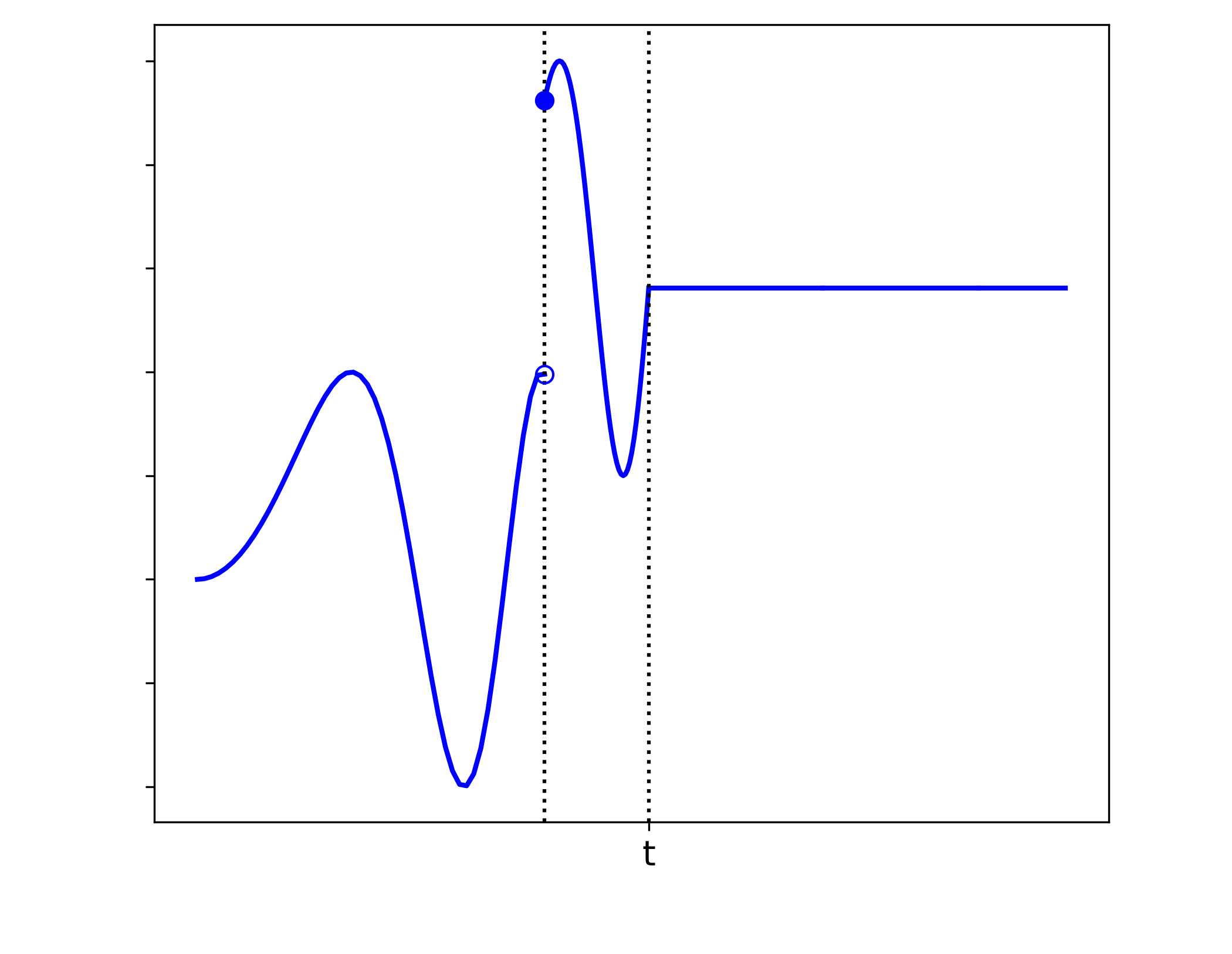
$\mathbf{X}^{[0]}$

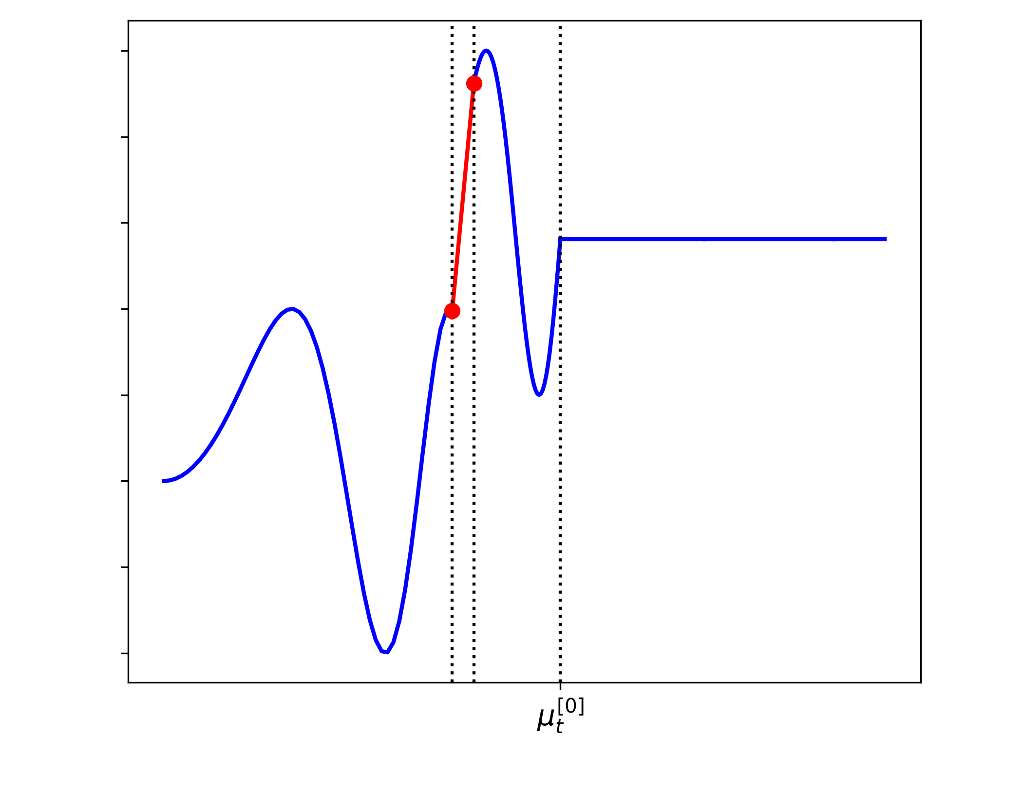
$\mathbf{Y}^{[0]}$

$$\begin{array}[]{l l}\text{Step I:}&\mathbf{X}^{[i_{2}]}(h_{2}):=\mathbf{Y}^{[0]}+h_{2}\epsilon_{i_{2}}1_{\{\cdot\geq\mu_{t}^{[0]}\}},\\ &\mathbf{Y}^{[i_{2}]}(h_{2}):=\ThisStyle{\stackengine{.8\LMpt}{\SavedStyle\mathbf{X}^{[i_{2}]}(h_{2})}{\stretchto{\scaleto{\SavedStyle\mkern 0.2mu\sim}{.5467}}{.5}}{O}{c}{F}{T}{S}},\\ &\mu_{t}^{[i_{2}]}(h_{2}):=\psi_{R_{2}}^{-1}(\tau_{\mathbf{X}^{[i_{2}]}(h_{2}),R_{2}}(\mu_{t}^{[0]})),\text{ for some pair }(R_{2},\psi_{R_{2}}).\end{array}$$

Figure 2: Step I

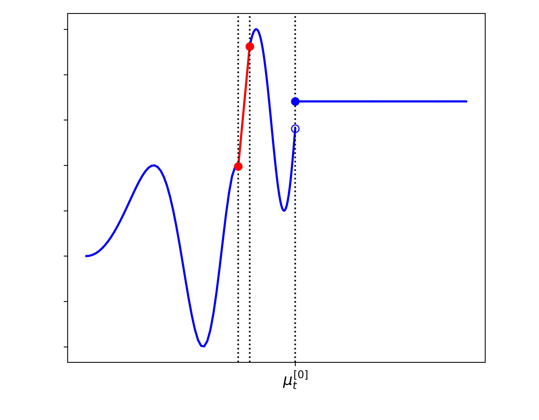
$\mathbf{X}^{[i_{2}]}(h_{2})$

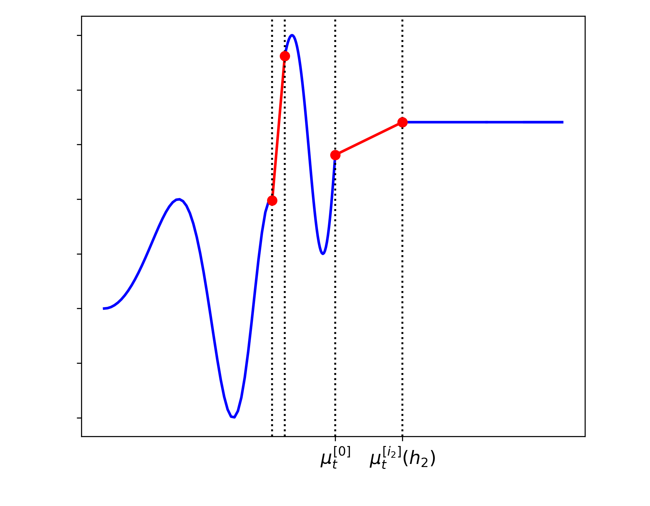
$\mathbf{Y}^{[i_{2}]}(h_{2})$

$$\begin{array}[]{l l}\text{Step II:}&\mathbf{X}^{[i_{2},i_{1}]}(h_{2},h_{1}):=\mathbf{Y}^{[i_{2}]}(h_{2})+h_{1}\epsilon_{i_{1}}1_{\{\cdot\geq\mu_{t}^{[i_{2}]}(h_{2})\}},\\ &\mathbf{Y}^{[i_{2},i_{1}]}(h_{2},h_{1}):=\ThisStyle{\stackengine{.8\LMpt}{\SavedStyle\mathbf{X}^{[i_{2},i_{1}]}(h_{2},h_{1})}{\stretchto{\scaleto{\SavedStyle\mkern 0.2mu\sim}{.5467}}{.5}}{O}{c}{F}{T}{S}},\\ &\mu_{t}^{[i_{2},i_{1}]}(h_{2},h_{1}):=\psi_{R_{1}}^{-1}(\tau_{\mathbf{X}^{[i_{2},i_{1}]}(h_{2},h_{1}),R_{1}}(\mu_{t}^{[i_{2}]}(h_{2})),\text{ for some pair }(R_{1},\psi_{R_{1}}).\end{array}$$

Figure 3: Step II

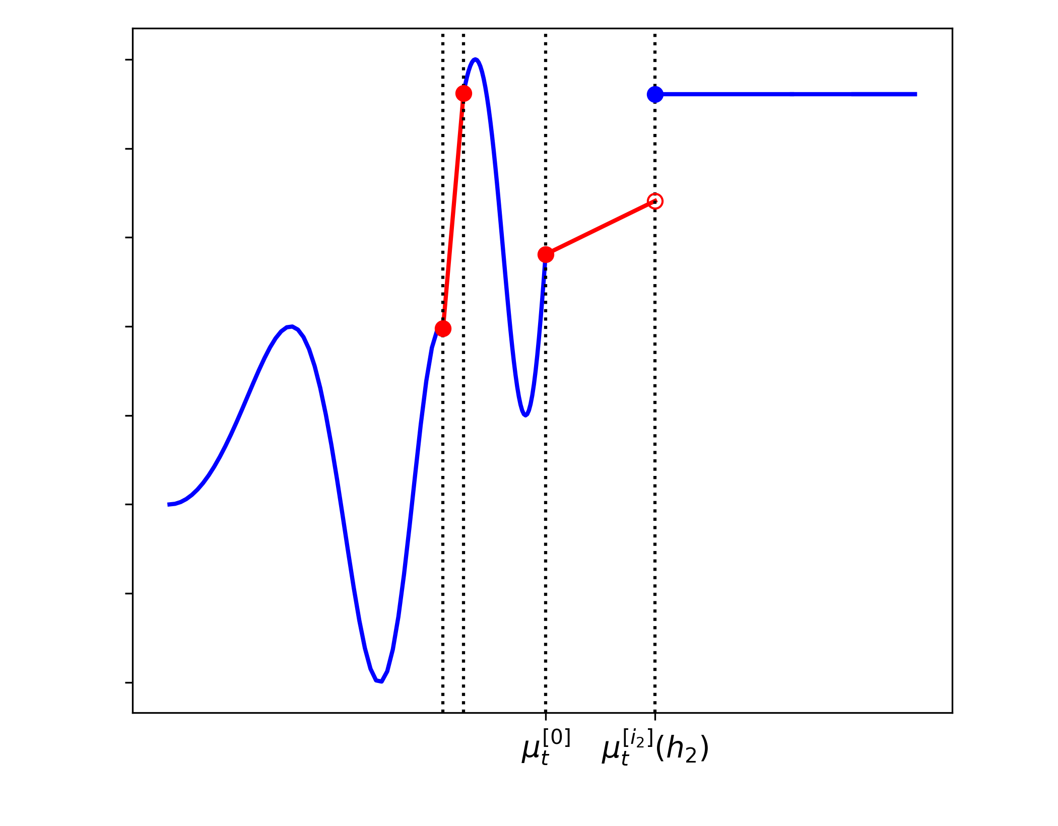
$\mathbf{X}^{[i_{2},i_{1}]}(h_{2},h_{1})$

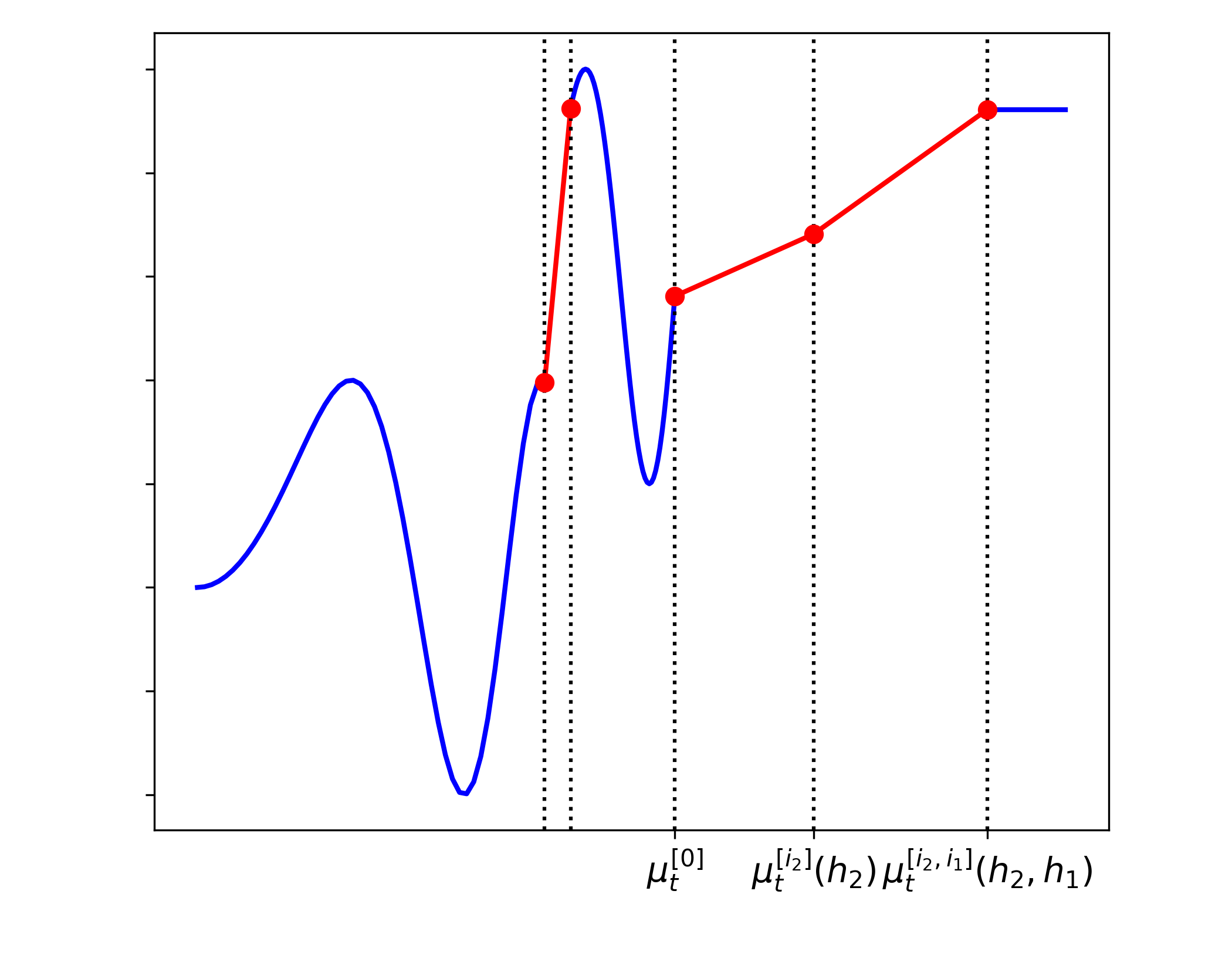
$\mathbf{Y}^{[i_{2},i_{1}]}(h_{2},h_{1})$

Notice that due to the one-dimensionality of the graphs, in Figures 1, 2, and 3 we consider a one-dimensional path and thus $i_{1}=i_{2}$.

Then, for $i_{1},i_{2}=1,\dots,d$,

$$U^{{i_{1}}}F(t,\mathbf{X})= \frac{d}{dh_{1}}F(\mu_{t}^{[i_{2},i_{1}]}(0,h_{1}),\mathbf{Y}^{[i_{2},i_{1}]}(0,h_{1}))|_{h_{1}=0},$$

$$U^{i_{2}}U^{i_{1}}F(t,\mathbf{X})= \frac{d^{2}}{dh_{2}dh_{1}}F(\mu_{t}^{[i_{2},i_{1}]}(h_{2},h_{1}),\mathbf{Y}^{[i_{2},i_{1}]}(h_{2},h_{1}))|_{h_{1}=h_{2}=0}.$$

In particular, if $i_{2}\neq i_{1}$, $U^{i_{2}}U^{i_{1}}F(t,\mathbf{X})$ and $U^{i_{1}}U^{i_{2}}F(t,\mathbf{X})$ are computed by evaluating the functional at different paths, that is,

$$U^{i_{2}}U^{i_{1}}F(t,\mathbf{X})= \frac{d^{2}}{dh_{2}dh_{1}}F(\mu_{t}^{[i_{2},i_{1}]}(h_{2},h_{1}),\mathbf{Y}^{[i_{2},i_{1}]}(h_{2},h_{1}))|_{h_{1}=h_{2}=0},$$ (3.7)

$$U^{i_{1}}U^{i_{2}}F(t,\mathbf{X})= \frac{d^{2}}{dh_{1}dh_{2}}F(\mu_{t}^{[i_{1},i_{2}]}(h_{1},h_{2}),\mathbf{Y}^{[i_{1},i_{2}]}(h_{1},h_{2}))|_{h_{1}=h_{2}=0},$$

with $\mathbf{Y}^{[i_{2},i_{1}]}(h_{2},h_{1}))$ and $\mathbf{Y}^{[i_{1},i_{2}]}(h_{1},h_{2}))$ being different. This is the crucial point as it is precisely for this reason that $U^{i_{2}}U^{i_{1}}F(t,\mathbf{X})$ and $U^{i_{1}}U^{i_{2}}F(t,\mathbf{X})$ are not necessarily equal, implying that the mixed vertical derivatives do not commute. One may notice that the derivatives with respect to $h_{1}$ and $h_{2}$ commute in each of the equations in (3.7) if the second order partial derivatives are continuous. However, this is not relevant. Indeed, the computation of different mixed vertical derivatives is not about reversing the order of differentiation with respect to $h_{1}$ and $h_{2}$, but, instead, requires evaluating the functional at different paths. This difference becomes more evident when recognizing that $\mathbf{Y}^{[i_{2},i_{1}]}(h_{2},h_{1})$ and $\mathbf{Y}^{[i_{1},i_{2}]}(h_{1},h_{2})$ are time-stretched versions of some Marcus transformation of the paths

$$\mathbf{X}^{t}+h_{2}\epsilon_{i_{2}}1_{\{\cdot\geq t+\varepsilon_{1}\}}+h_{1}\epsilon_{i_{1}}1_{\{\cdot\geq t+\varepsilon_{1}+\varepsilon_{2}\}},$$ (3.8)

$$\mathbf{X}^{t}+h_{1}\epsilon_{i_{1}}1_{\{\cdot\geq t+\varepsilon_{1}\}}+h_{2}\epsilon_{i_{2}}1_{\{\cdot\geq t+\varepsilon_{1}+\varepsilon_{2}\}},$$

respectively, and that by conditions (ii),(iii) in Definition 3.4,

$$U^{i_{2}}U^{i_{1}}F(t,\mathbf{X})= \frac{d^{2}}{dh_{2}dh_{1}}F(t+\varepsilon_{1}+\varepsilon_{2},\mathbf{X}^{t}+h_{2}\epsilon_{i_{2}}1_{\{\cdot\geq t+\varepsilon_{1}\}}+h_{1}\epsilon_{i_{1}}1_{\{\cdot\geq t+\varepsilon_{1}+\varepsilon_{2}\}})|_{h_{1}=h_{2}=0}.$$

$$U^{i_{1}}U^{i_{2}}F(t,\mathbf{X})= \frac{d^{2}}{dh_{1}dh_{2}}F(t+\varepsilon_{1}+\varepsilon_{2},\mathbf{X}^{t}+h_{1}\epsilon_{i_{1}}1_{\{\cdot\geq t+\varepsilon_{1}\}}+h_{2}\epsilon_{i_{2}}1_{\{\cdot\geq t+\varepsilon_{1}+\varepsilon_{2}\}})|_{h_{1}=h_{2}=0}.$$

Therefore, computing the mixed vertical derivatives reduces in fact to considering different delayed perturbations. In particular, in the calculation of $U^{i_{2}}U^{i_{1}}F(t,\mathbf{X})$ the path is vertically perturbed first in the direction of the canonical vector $\epsilon_{i_{2}}$, followed by a perturbation in the direction of $\epsilon_{i_{1}}$, which results in

$$\frac{d}{dh_{1}}F(t+\varepsilon_{1}+\varepsilon_{2},\mathbf{X}^{t}+h_{2}\epsilon_{i_{2}}1_{\{\cdot\geq t+\varepsilon_{1}\}}+h_{1}\epsilon_{i_{1}}1_{\{\cdot\geq t+\varepsilon_{1}+\varepsilon_{2}\}})|_{h_{1}=0} =U^{i_{1}}F(t+\varepsilon_{1},\mathbf{X}^{t}+h_{2}\epsilon_{i_{2}}1_{\{\cdot\geq t+\varepsilon_{1}\}})$$

$$\frac{d}{dh_{2}}U^{i_{1}}F(t+\varepsilon_{1},\mathbf{X}^{t}+h_{2}\epsilon_{i_{2}}1_{\{\cdot\geq t+\varepsilon_{1}\}})|_{h_{2}=0} =U^{i_{2}}U^{i_{1}}F(t,\mathbf{X}).$$

In the calculation of $U^{i_{1}}U^{i_{2}}F(t,\mathbf{X})$ instead, the order of the vertical perturbation of the path is reversed. To clarify this argument further, we illustrate in Figure 4 the vertical perturbations of a 2-dimensional path. The image on the left shows the perturbation required for computing $U^{2}U^{1}F(t,\mathbf{X})$, while the image on the right the perturbation for computing $U^{1}U^{2}F(t,\mathbf{X})$.

Figure 4: Vertically perturbed $2$-dimensional path

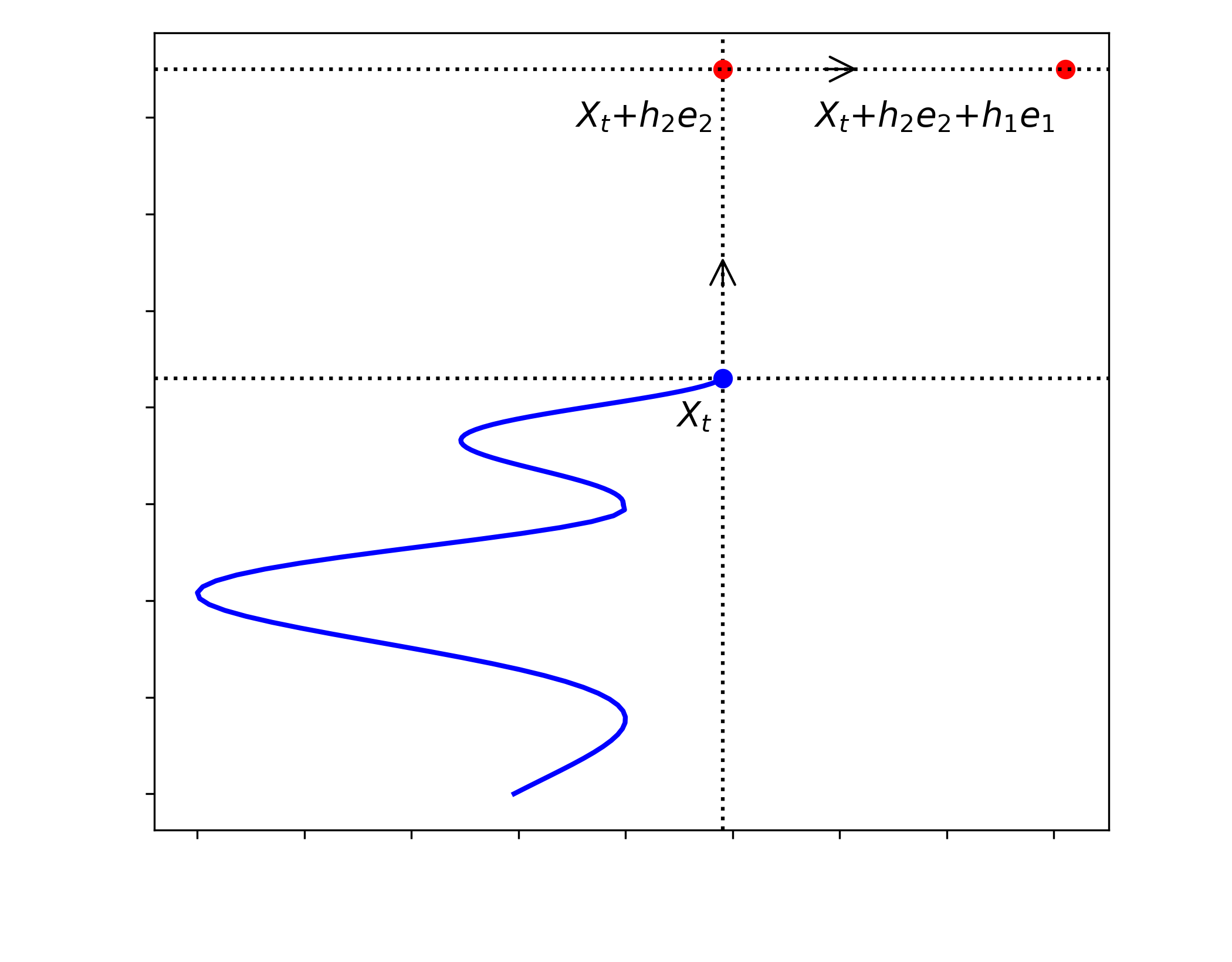
$\mathbf{X}^{t}+h_{2}\epsilon_{2}1_{\{\cdot\geq t+\varepsilon_{2}\}}+h_{1}\epsilon_{1}1_{\{\cdot\geq t+\varepsilon_{2}+\varepsilon_{1}\}}$

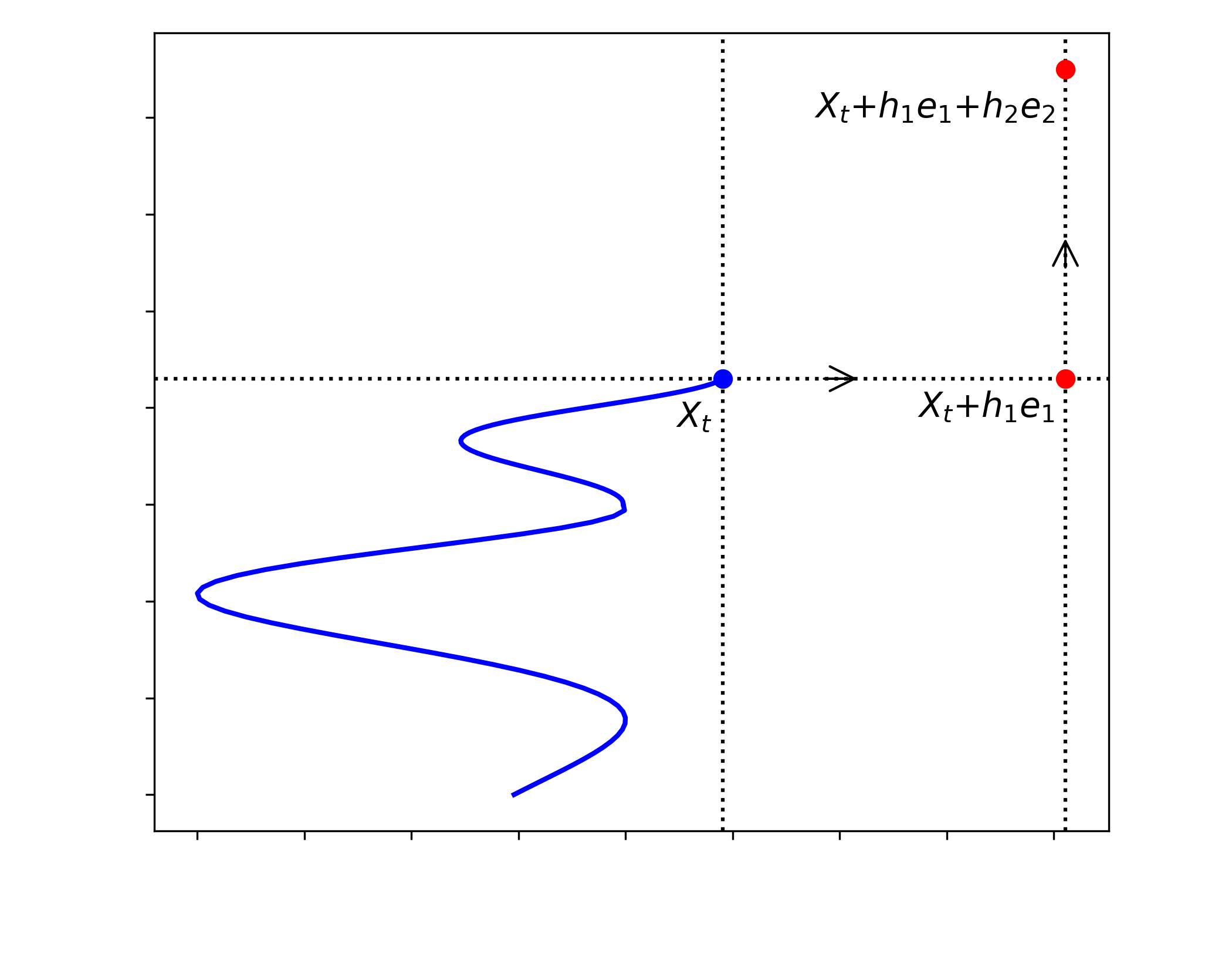
$\mathbf{X}^{t}+h_{1}\epsilon_{1}1_{\{\cdot\geq t+\varepsilon_{1}\}}+h_{2}\epsilon_{2}1_{\{\cdot\geq t+\varepsilon_{1}+\varepsilon_{2}\}}$

Example 3.19.

Let us consider the path functional introduced in Example 3.8(iii), that is

$$F(t,\mathbf{X}):=\int_{0}^{t}\mathbf{X}^{1}_{s^{-}}d\mathbf{X}^{2}_{s}+\frac{1}{2}\sum_{0<s\leq t}\Delta\mathbf{X}^{1}_{s}\Delta\mathbf{X}^{2}_{s},$$

for all $(t,\mathbf{X})\in D^{1}([0,1],G^{1}(\mathbb{R}^{2}))$.

A direct computation of the iterative procedure described above shows that for all $(t,\mathbf{X})\in[0,1]\times D([0,1],G^{1}(\mathbb{R}^{2}))$, one gets

$$U^{2}U^{2}F(t,\mathbf{X})=U^{1}U^{1}F(t,\mathbf{X})=U^{2}U^{1}F(t,\mathbf{X})=U^{1}F(t,\mathbf{X})=0,$$

whereas,

$$U^{2}F(t,\mathbf{X})=\mathbf{X}^{1}_{t}\quad\text{and}\quad U^{1}U^{2}F(t,\mathbf{X})=1.$$

Remark 3.20.

The above considerations, in particular Example 3.19, show that the notion of vertical derivatives of higher order introduced in Definition 3.17 establishes a differential calculus for path functionals that allows for non-commutative derivation orders. This is in contrast to the setup in Dupire (2009), Cont and Fournie (2010a), Cont et al. (2016) (see e.g., p. 133 in Cont et al. (2016)).

This different behavior can be explained as follows. For a path functional that is non-anticipative, the second-order vertical derivatives at some $(t,\mathbf{X})$ as computed in Dupire (2009) (see also Definition 9 in Cont and Fournie (2013)) explicitly read as

$$\partial_{i_{2}}\partial_{i_{1}}F(t,\mathbf{X})= \frac{d^{2}}{dh_{2}dh_{1}}F(t,\mathbf{X}^{t}+(h_{2}\epsilon_{i_{2}}+h_{1}\epsilon_{i_{1}})1_{\{\cdot\geq t\}})|_{h_{1}=h_{2}=0},$$ (3.9)

for $i_{1},i_{2}=1,\dots,d$. In contrast, in the present framework,

$$U^{i_{2}}U^{i_{1}}F(t,\mathbf{X})=\frac{d^{2}}{dh_{2}dh_{1}}F(t+\varepsilon_{2}+\varepsilon_{1},\mathbf{X}^{t}+h_{2}\epsilon_{i_{2}}1_{\{\cdot\geq t+\varepsilon_{2}\}}+h_{1}\epsilon_{i_{1}}1_{\{\cdot\geq t+\varepsilon_{2}+\varepsilon_{1}\}})|_{h_{1}=h_{2}=0}.$$

As already argued above this means that, if $i_{1}\neq i_{2}$, $U^{i_{2}}U^{i_{1}}F(t,\mathbf{X})$ and $U^{i_{1}}U^{i_{2}}F(t,\mathbf{X})$ are computed by evaluating the functional at different paths. This differs from the computation in (3.9) where, since the perturbation occurs at the same time, the functional is evaluated always at the same path. Observe furthermore that

$$\partial_{i_{2}}\partial_{i_{1}}F(t,\mathbf{X})=\partial^{2}_{\xi_{i_{1}}\xi_{i_{2}}}G(\xi)|_{\xi=0},$$

for $G(\xi):=F(t,\mathbf{X}+\xi 1_{\{\cdot\geq t\}})$, $\xi\in\mathbb{R}^{d}$. Therefore, by Schwarz’s theorem the mixed vertical derivatives as computed in Dupire (2009) are equal as long as the maps $\xi\mapsto\partial^{2}_{\xi_{i_{1}}\xi_{i_{2}}}G(\xi)$ are continuous in a neighborhood of $0$. Other considerations for accommodating the non-communicative nature of the higher-order derivatives have been made by Dupire and Saporito (2019).

The non-commutative behavior that we obtain here is particularly relevant when dealing with weakly geometric $p$-rough paths, for $p\in[2,3)$, where the second order vertical derivatives appear in the Itô-formula (see Sections 5.2). It is, however, also crucial for finite variation paths in view of the Taylor expansions (see Theorem 6.1).

3.3 Var-continuous path functionals

In this section, we introduce the necessary regularity conditions for the path functionals to derive the results presented in the subsequent sections. Unless otherwise specified, we let $p\in[1,3)$ and for $q\geq p$, we denote by $d_{q}$ the $q$-variation pseudometric on the space of càdlàg paths as defined in Section 2.2.

Definition 3.21.

Fix $m\in\mathbb{N}_{0}$. We say that a path functional $F\in((\mathcal{M}_{[p]}^{0})^{d})^{\otimes m}$ is $[p,[p]+1)$-var continuous if for every $(\mathbf{X}^{n},\mathbf{X})_{n\in\mathbb{N}}\subset C^{p}([0,1],G^{[p]}(\mathbb{R}^{d}))$ such that for some $q\in[p,[p]+1)$

$$\lim_{n\rightarrow\infty}d_{q}(\mathbf{X}^{n},\mathbf{X})=0,$$

it holds that

$$\lim_{n\rightarrow\infty}d_{q^{\prime}}(F(\cdot,\mathbf{X}^{n}),F(\cdot,\mathbf{X}))=0,$$

for all $q^{\prime}>q$.

Definition 3.22.

Fix $m\in\mathbb{N}_{0}$. For $p\in[2,3)$ and $F\in((\mathcal{M}_{2}^{0})^{d})^{\otimes m}$, $F^{\prime}\in((\mathcal{M}_{2}^{0})^{d})^{\otimes m+1}$, we say that a remainder path functionals $R^{F,F^{\prime}}$, defined in Definition 3.12, is $[p,3)$-var continuous if for every $(\mathbf{X}^{n},\mathbf{X})_{n\in\mathbb{N}}\subset C^{p}([0,1],G^{2}(\mathbb{R}^{d}))$ such that for some $q\in[p,3)$

$$\lim_{n\rightarrow\infty}d_{q}(\mathbf{X}^{n},\mathbf{X})=0,$$

it holds that

$$\lim_{n\rightarrow\infty}d_{q^{\prime}/2}(R((\cdot,\cdot),\mathbf{X}^{n}),R((\cdot,\cdot),\mathbf{X}))=0,$$

for all $q^{\prime}>q$.

3.4 Linear functionals of the signature

This section is devoted to the study of linear functionals of the signature.

Definition 3.23.

Fix $\mathbf{u}\in T(\mathbb{R}^{d})$. We call the path functional

$$F^{\mathbf{u}}: [0,1]\times D^{p}([0,1],G^{[p]}(\mathbb{R}^{d}))\rightarrow\mathbb{R}$$ (3.10)

$$\quad(t,\mathbf{X})\longmapsto F^{\mathbf{u}}(t,\mathbf{X}):=\langle\mathbf{u},\mathbb{X}_{t}\rangle$$

linear functional of the signature.

The proof of the following proposition is given in Appendix A.3.

Proposition 3.24.

Let $F^{\mathbf{u}}:[0,1]\times D^{p}([0,1],G^{[p]}(\mathbb{R}^{d}))\rightarrow\mathbb{R}$ be a linear functionals of the signature for some $\mathbf{u}\in T(\mathbb{R}^{d})$. Then,

1. $F^{\mathbf{u}}$ is a non-anticipative Marcus canonical path functional.

2. $F^{\mathbf{u}}$ is infinitely many times vertically differentiable and for all $k\in\mathbb{N}$,

   $$\nabla^{k}F^{\mathbf{u}}(t,\mathbf{X})=\langle\mathbf{u}^{(k)},\mathbb{X}_{t}\rangle,$$ (3.11)

   for all $(t,\mathbf{X})\in[0,1]\times D([0,1],G^{[p]}(\mathbb{R}^{d}))$.

3. $F^{\mathbf{u}}$ is $[p,[p]+1)$-var continuous.

Now, a direct combination of Proposition 3.24 and equations (2.18) and (2.19) yields the functional Itô-formula for linear functionals of the signature.

Lemma  3.25.

Let $F^{\mathbf{u}}:[0,1]\times D^{p}([0,1],G^{[p]}(\mathbb{R}^{d}))\rightarrow\mathbb{R}$ be a linear functional of the signature for some $\mathbf{u}\in T(\mathbb{R}^{d})$. Then, the following functional Itô-formulas hold.

1. If $p\in[1,2)$,

   $$F^{\mathbf{u}}(t,\mathbf{X})= F^{\mathbf{u}}(0,\mathbf{X})+\int_{0}^{t}\nabla F^{\mathbf{u}}(s^{-},\mathbf{X})d\mathbf{X}_{s}$$

   $$+\sum_{0<s\leq t}F^{\mathbf{u}}(s,\mathbf{X})-F^{\mathbf{u}}(s^{-},\mathbf{X})-\Delta F^{\mathbf{u}}(s^{-},\mathbf{X})\Delta X_{s}.$$

   The integral term is a Young integral of $\nabla F^{\mathbf{u}}(\cdot,\mathbf{X})\in D^{p}([0,1],\mathbb{R}^{d+1})$ with respect to $\mathbf{X}$.

2. If $p\in[2,3)$,

   $$F^{\mathbf{u}}(t,\mathbf{X})= F^{\mathbf{u}}(0,\mathbf{X})+\int_{0}^{t}F^{\mathbf{u}}(s^{-},\mathbf{X})d\mathbf{X}_{s}$$

   $$+\sum_{0<s\leq t}F^{\mathbf{u}}(s,\mathbf{X})-F^{\mathbf{u}}(s^{-},\mathbf{X})-\nabla F^{\mathbf{u}}(s^{-},\mathbf{X})\Delta X_{s}-\nabla^{2}F^{\mathbf{u}}(s^{-},\mathbf{X})\Delta\mathbb{X}^{(2)}_{s}.$$

   The integral term is a rough integral of $\big{(}\nabla F^{\mathbf{u}}(\cdot,\mathbf{X}),\nabla^{2}F^{\mathbf{u}}(\cdot,\mathbf{X})\big{)}\in\mathcal{V}^{p,\frac{p}{2}}_{\mathbf{X}}$ with respect to $\mathbf{X}$.

4 Universal approximation theorem for vertically differentiable path functionals

In this section, we exploit the approximation properties of the signature of weakly geometric càdlàg $p$ rough paths to derive a universal approximation theorem (UAT) for non-anticipative Marcus canonical path functionals which are vertically differentiable (Theorem 4.14).

This result for path functionals is analogous to the classic Nachbin theorem, which provides an analog to the Stone-Weierstrass theorem for algebras of $C^{K}$ functions on $\mathbb{R}^{d}$, for $K\in\mathbb{N}$ (see Nachbin (1949)).

4.1 The subspace of the tracking-jumps-extended paths

First, we introduce the subset of paths considered for deriving the UAT. We call them tracking jumps-extended paths. The distinctive feature of these paths is that they always admit a Marcus transformed path that is time-extended (see Remark 4.5(ii)). This is a key aspect both for the development of the proof of Theorem 4.14 and the main results in Sections 5 and 6.

The notion of tracking jumps-extended paths relies on the more general one of extended weakly geometric càdlàg rough path, which we give below. Roughly speaking this space consists of all the weakly geometric càdlàg $p$-rough paths with values in $G^{[p]}(\mathbb{R}^{d+1})$ obtained through the addition of an auxiliary path component of finite variation to some $\mathbf{X}\in D^{p}([0,1],G^{[p]}(\mathbb{R}^{d}))$. When $p\in[1,2)$, this extension is quite straightforward. When $p\in[2,3)$ instead, one needs to ensure consistency between the Young and the (level 2) rough integration (see Section E.1), while preserving the group-valued constraint. For the explanation of the index $0$ used here we refer to Notation 4.2 below.

Definition 4.1.

Fix $Z\in D^{1}([0,1],\mathbb{R})$ and $\widehat{\mathbf{X}}\in D^{p}([0,1],G^{[p]}(\mathbb{R}^{d+1})).$

1. If $p\in[1,2)$, we say that $\widehat{\mathbf{X}}$ is a $Z$-extended weakly geometric càdlàg $p$-rough path if for all $i=1,\dots,d$,

   $$\langle\epsilon_{i},\widehat{\mathbf{X}}\rangle=\langle\epsilon_{i},\mathbf{X}\rangle,\quad\text{and }\quad\langle\epsilon_{0},\widehat{\mathbf{X}}\rangle=Z,$$

   for some $\mathbf{X}\in D^{p}([0,1],G^{1}(\mathbb{R}^{d}))$.

2. If $p\in[2,3)$, we say that $\widehat{\mathbf{X}}$ is a $Z$-extended weakly geometric càdlàg $p$-rough path if for all $i,j=1,\dots,d$,

   $$\langle\epsilon_{i},\widehat{\mathbf{X}}\rangle=\langle\epsilon_{i},\mathbf{X}\rangle,\qquad\langle\epsilon_{(ji)},\widehat{\mathbf{X}}\rangle=\langle\epsilon_{(ji)},\mathbf{X}\rangle,\qquad\langle\epsilon_{0},\widehat{\mathbf{X}}\rangle=Z,$$

   and for all $i=0,\dots,d$,

   $$\langle\epsilon_{(i,0)},\widehat{\mathbf{X}}\rangle=\int_{0}^{\cdot}\langle\epsilon_{i},\widehat{\mathbf{X}}_{0,s^{-}}\rangle dZ_{s}+\frac{1}{2}\sum_{0<s\leq\cdot}\Delta\langle\epsilon_{i},\widehat{\mathbf{X}}_{s}\rangle\Delta Z_{s}.$$ (4.1)

   for some $\mathbf{X}\in D^{p}([0,1],G^{2}(\mathbb{R}^{d}))$, and the integral in (4.1) is of Young type.

Notation 4.2.

Unless explicitly mentioned, we use throughout the paper the index $0$ to denote the additional auxiliary component $Z$ of $\widehat{\mathbf{X}}$.

Remark 4.3.

1. Let $p\in[2,3)$. Notice that by definition any $Z$-extended weakly geometric càdlàg $p$-rough path $\widehat{\mathbf{X}}$ lies in $G^{2}(\mathbb{R}^{d+1})$. Therefore, by the shuffle property (2.8), for all $i=0,1,\dots,d$, $t\in[0,1]$,

   $$\langle\epsilon_{(0,i)},\widehat{\mathbf{X}}_{t}\rangle=Z_{t}\langle\epsilon_{i},\widehat{\mathbf{X}}_{t}\rangle-\langle\epsilon_{(i,0)},\widehat{\mathbf{X}}_{t}\rangle.$$

   Moreover, since $Z\in D^{1}([0,1],\mathbb{R})$ and $\langle\epsilon_{i},\mathbf{X}\rangle\in D^{p}([0,1],\mathbb{R})$, the Young integral in (4.1) is well defined and for all $t\in[0,1]$,

   $$\sum_{0<s\leq t}|\Delta\langle\epsilon_{i},\widehat{\mathbf{X}}_{s}\rangle\Delta Z_{s}|\leq\left(\sum_{0<s\leq t}|\Delta\langle\epsilon_{i},\widehat{\mathbf{X}}_{s}\rangle|^{3}\right)^{1/3}\left(\sum_{0<s\leq t}|\Delta Z_{s}|^{\frac{3}{2}}\right)^{2/3}<\infty.$$

   This implies that the path defined in equation (4.1) is of finite variation and the definition is well-posed.

2. One can see that given $Z\in D^{1}([0,1],\mathbb{R})$ and $\mathbf{X}\in D^{p}([0,1],G^{[p]}(\mathbb{R}^{d}))$, it is always possible to build a $Z$-extended weakly geometric $p$-rough path $\widehat{\mathbf{X}}$ as in Definition 4.1. The reverse is trivially true.

Now, we are ready to introduce the set of tracking jumps-extended paths.

Definition 4.4.

We say that $\widehat{\mathbf{X}}\in{D}^{p}([0,1],G^{[p]}(\mathbb{R}^{d+1}))$ is a tracking-jumps-extended weakly geometric càdlàg $p$-rough path if it is the $Z$-extension of some $\mathbf{X}\in{D}^{p}([0,1],G^{[p]}(\mathbb{R}^{d}))$, for a càdlàg strictly increasing piecewise linear function $Z:[0,1]\rightarrow[0,1]$ such that $Z_{0}=0$, $Z_{1}=1$, and

$$\{s\in(0,1]\ :\ \Delta Z_{s}\neq 0\}=\{s\in(0,1]\ :\ \Delta\mathbf{X}_{s}\neq 0\}.$$

We call such a path $Z$ tracking-jumps-path of $\mathbf{X}$ and denote the set of such $Z$-extended càdlàg

(continuous) paths by $\widehat{D}^{p}([0,1],G^{[p]}(\mathbb{R}^{d+1}))$ ($\widehat{C}^{p}([0,1],G^{[p]}(\mathbb{R}^{d+1}))$).

Remark 4.5.

1. Given $\mathbf{X}\in{D}^{p}([0,1],G^{[p]}(\mathbb{R}^{d}))$ it is always possible to build (non-uniquely) a tracking-jumps path associated with it. If $\mathbf{X}$ is continuous, the tracking-jumps path is unique and given by the identity path $\text{Id}_{u}:=u$ for all $u\in[0,1]$. For $\mathbf{X}$ càdlàg , there exists more than one tracking-jumps-extension $\widehat{\mathbf{X}}$. We refer to every Id-extended continuous path as time-extended path.

   Notice in particular that the existence of a tracking-jumps-extension is related only to the càdlàg property of the original path.

2. Observe that for all $\widehat{\mathbf{X}}\in\widehat{D}^{p}([0,1],G^{[p]}(\mathbb{R}^{d+1}))$ there always exists a Marcus-transformed path of $\widehat{\mathbf{X}}$ with respect to some pair $(R,\psi_{R})$, which is a time-extended weakly geometric continuous $p$-rough path. Indeed, since a tracking-jumps path is simply a strictly increasing piecewise linear path $Z$ such that $Z(0)=0$ and $Z(1)=1$ and jumps whenever the other components of the path do, a pair $(R,\psi_{R})$ can be chosen to ensure a Marcus-transformed path for which the transformed component $\widetilde{Z}$ satisfies $\widetilde{Z}_{u}=u$ for all $u\in[0,1]$.

4.2 UAT for vertically differentiable path functionals

To present the main result of the section (Theorem 4.14), we shall introduce some notation and new definitions. Since we will be mostly concerned with paths with values in $G^{[p]}(\mathbb{R}^{d+1})$, we introduce the relevant notions by considering directly the space $\mathbb{R}^{d+1}$.

Notation 4.6.

Let $K\in\mathbb{N}$ and $\mathfrak{g}^{K}(\mathbb{R}^{d+1})$ be the free step-$K$ nilpotent Lie algebra over $\mathbb{R}^{d+1}$ (see Section 2.1). Recall that for every $\boldsymbol{\xi}:=(0,\boldsymbol{\xi}^{(1)},\dots,\boldsymbol{\xi}^{(K)})\in\mathfrak{g}^{K}(\mathbb{R}^{d+1})$,

$$\boldsymbol{\xi}^{(j)}:=\pi_{j}(\boldsymbol{\xi})\in\underbrace{[\mathbb{R}^{d+1},[\mathbb{R}^{d+1},\dots,[\mathbb{R}^{d+1},\mathbb{R}^{d+1}]]]}_{(j-1)\text{ brackets}},$$

for $j=1,\dots,K$. Set $M:=\text{dim}(\mathfrak{g}^{K}(\mathbb{R}^{d+1}))=\sum_{j=1}^{K}M_{j}$ and

$$M_{j}:=\text{dim}(\underbrace{[\mathbb{R}^{d+1},[\mathbb{R}^{d+1},\dots,[\mathbb{R}^{d+1},\mathbb{R}^{d+1}]]]}_{(j-1)\text{ brackets}}).$$

For $\beta\in\mathbb{N}_{0}^{M}$, we write $\beta=(\beta_{1},\dots,\beta_{K})$, with $\beta_{j}\in\mathbb{N}_{0}^{M_{j}}$, and set

$$|\beta|:=\sum_{j=1}^{K}\sum_{i=1}^{M_{j}}\beta^{i}_{j},\qquad\text{and}\quad|\beta|_{\mathfrak{g}^{K}(\mathbb{R}^{d+1})}:=\sum_{j=1}^{K}\sum_{i=1}^{M_{j}}j\beta^{i}_{j}.$$ (4.2)

Furthermore, let $\partial^{\beta_{j}}_{\boldsymbol{\xi}^{(j)}}$ denote the differential operator such that

$$\partial^{\beta_{j}}_{\boldsymbol{\xi}^{(j)}}f(\boldsymbol{\xi}):=\frac{\partial^{|\beta_{j}|}f}{\partial^{\beta_{j}^{1}}\boldsymbol{\xi}^{(j),1}\dots\partial^{\beta_{j}^{M_{j}}}\boldsymbol{\xi}^{(j),M_{j}}}(\boldsymbol{\xi}),$$

for $\boldsymbol{\xi}^{(j),l}$ denoting the $l$-th component of $\boldsymbol{\xi}^{(j)}$, $|\beta_{j}|:=\sum_{i=1}^{M_{j}}\beta^{i}_{j}$, and $f:\mathcal{U}\rightarrow\mathbb{R}$ some sufficiently regular map defined on some open set $\mathcal{U}\subseteq\mathfrak{g}^{K}(\mathbb{R}^{d+1})$, with $\boldsymbol{\xi}\in\mathcal{U}$.

Finally, denote by $D^{\beta}_{\boldsymbol{\xi}}:=\partial_{\boldsymbol{\xi}^{(1)}}^{\beta_{1}}\dots\partial_{\boldsymbol{\xi}^{(K)}}^{\beta_{K}}$ the operator given by a consecutive application of $\partial_{\boldsymbol{\xi}^{(1)}}^{\beta_{1}},\dots,\partial_{\boldsymbol{\xi}^{(K)}}^{\beta_{K}}$.

Recall that $G((\mathbb{R}^{d+1}))$ denotes the set of group-like elements, introduced in equation (2.6).

Assumption 4.7.

$F:[0,1]\times D^{p}([0,1],G^{[p]}(\mathbb{R}^{d+1}))\rightarrow\mathbb{R}$ is a Marcus canonical non-anticipative path functional such that for all $(t,\mathbf{X})\in[0,1]\times{C}^{p}([0,1],G^{[p]}(\mathbb{R}^{d+1}))$,

$$F(t,\mathbf{X})=g(\mathbb{X}_{t}),$$ (4.3)

for some $g:G((\mathbb{R}^{d+1}))\rightarrow\mathbb{R}$, and $\mathbb{X}$ denoting the signature of $\mathbf{X}$.

Remark 4.8.

1. By the definition of Marcus canonical path functionals and the signature of càdlàg rough paths, the equality (4.3) is valid in fact on $[0,1]\times{D}^{p}([0,1],G^{[p]}(\mathbb{R}^{d+1}))$.

2. Let $S$ be the map such that for all $\mathbf{X}\in{C}^{p}([0,1],G^{[p]}(\mathbb{R}^{d+1}))$, $S(\mathbf{X}):=\mathbb{X}_{1}$. For $t\in[0,1]$, let $\widehat{C}^{p}_{t}([0,1],G^{[p]}(\mathbb{R}^{d+1}))$ denote the space of time-extended paths stopped at time $t$. One can show that on the set

   $$\bigcup_{t\in[0,1]}\widehat{C}_{t}^{p}([0,1],G^{[p]}(\mathbb{R}^{d+1}))$$

   $S$ is an injective map (see e.g., the proof of Proposition 3.6 in Cuchiero et al. (2025)). Therefore, the restriction of the map $S$ to its image, denoted as $\mathcal{S}$, is a bijection. Furthermore, consider the map $\widetilde{F}:\bigcup_{t\in[0,1]}\widehat{C}_{t}^{p}([0,1],G^{[p]}(\mathbb{R}^{d+1}))\rightarrow\mathbb{R}$ given by $\widetilde{F}(\widehat{\mathbf{X}}^{t}):=F(t,\widehat{\mathbf{X}}^{t})$ and notice that $F$ admits a representation of the form

   $$F(t,\widehat{\mathbf{X}}^{t})=\bar{g}(\widehat{\mathbb{X}}_{t}),$$ (4.4)

   for $\bar{g}:\mathcal{S}\rightarrow\mathbb{R}$ given by $\bar{g}:=\widetilde{F}\circ S^{-1}$ and every (stopped) time-extended continuous path $\widehat{\mathbf{X}}^{t}$. Notice that the above reasoning applies in fact to the larger set of càdlàg paths. However, in general, the set $\mathcal{S}\subsetneq G((\mathbb{R}^{d+1}))$ might not be big enough for the application of the reasonings in the proofs of Lemma 4.9 and Theorem 4.14, which involve some ideas from Lie group theory (see Bonfiglioli et al. (2007)).

The proof of the following lemma is given in Appendix B.1.

Lemma  4.9.

Let $F\in\mathcal{M}_{[p]}^{K}$, for some $K\in\mathbb{N}$. Fix $\mathbf{X}\in[0,1]\times C^{p}([0,1],G^{[p]}(\mathbb{R}^{d}))$ and denote by $\mathbb{X}$ its signature. Under Assumption 4.7, the map

$$g^{\mathbf{X},K}: [0,1]\times\mathfrak{g}^{K}(\mathbb{R}^{d+1})\rightarrow\mathbb{R}$$ (4.5)

$$\qquad(t,\boldsymbol{\xi})\mapsto g^{\mathbf{X},K}(t,\boldsymbol{\xi}):=g(\mathbb{X}_{t}\otimes\exp(\boldsymbol{\xi},0\dots,0))$$

is well defined and its derivatives at zero $D^{\beta}_{\boldsymbol{\xi}}g^{\mathbf{X},K}(t,\boldsymbol{\xi})|_{\boldsymbol{\xi}=0}$ exist for all $|\beta|_{\mathfrak{g}^{K}(\mathbb{R}^{d+1})}\leq K$.

For the development of the following results, we need the map $g^{\mathbf{X},K}$ to satisfy some stronger continuity conditions in the next assumption.

Assumption 4.10.

For all $\mathbf{X}\in C^{p}([0,1],G^{[p]}(\mathbb{R}^{d}))$, the map

$$[0,1]\times\mathcal{U}(0)\ni(t,\boldsymbol{\xi})\mapsto D^{\beta}_{\boldsymbol{\xi}}g^{\mathbf{X},K}(t,\boldsymbol{\xi})$$

is jointly continuous for all $|\beta|_{\mathfrak{g}^{K}(\mathbb{R}^{d+1})}\leq K$, and some open neighborhood $\mathcal{U}(0)$ of $0\in\mathfrak{g}^{K}(\mathbb{R}^{d+1})$.

Remark 4.11.

Under Assumption 4.10, the map $\mathcal{U}(0)\ni\boldsymbol{\xi}\mapsto D^{\beta}g^{\mathbf{X},K}(t,\boldsymbol{\xi})$ does not depend on the order of the partial derivatives (see Step 2 in the proof of Theorem 4.14).

Definition 4.12.

Let $F:[0,1]\times D^{p}([0,1],G^{[p]}(\mathbb{R}^{d+1}))\rightarrow\mathbb{R}$. We write $F\in C^{K}$ if $F\in\mathcal{M}_{[p]}^{K}$ and Assumptions 4.7 and 4.10 are satisfied.

An example of path functional satisfying the assumptions of Definition 4.12 is given by the linear functionals of the signature $F^{\mathbf{u}}$, for some $\mathbf{u}\in T(\mathbb{R}^{d+1})$ (see Section 3.4). Then, by Proposition 3.24 $F^{\mathbf{u}}\in C^{K}$ for all $K\in\mathbb{N}$, and the map (4.5) explicitly reads as

$$g^{\mathbf{X},K}(t,\boldsymbol{\xi}):=\langle\mathbf{u},\mathbb{X}_{t}\otimes\exp(\boldsymbol{\xi},0\dots,0)\rangle,$$

for all $(t,\boldsymbol{\xi})$ and $\mathbf{X}$.

Remark 4.13.

For $m\in\mathbb{N}_{0}$, $K\in\mathbb{N}$ and a $(\mathbb{R}^{d})^{\otimes m}$-valued path functional $F$, we write $F\in C^{K}$ if its components are $C^{K}$. Notice that if $F\in C^{K}$, then for all $l=1,\dots,K$, $\nabla^{l}F\in C^{K-l}$.

Now we state the main result of the section stating that any path functionals $F\in C^{K}$ when evaluated at a tracking jumps-extended path $\widehat{\mathbf{X}}$ (Definition 4.4), can be uniformly approximated in time, along with its derivatives, by linear functionals of the signature and its derivatives.

Theorem 4.14.

Let $F:[0,1]\times D^{p}([0,1],G^{[p]}(\mathbb{R}^{d+1}))\rightarrow\mathbb{R}$. Assume $F\in C^{K}$. Then, for all $\widehat{\mathbf{X}}\in\widehat{D}^{p}([0,1],G^{[p]}(\mathbb{R}^{d+1}))$ there exists $(\mathbf{u}_{n})_{n\in\mathbb{N}}\in T(\mathbb{R}^{d+1})$ (possibly depending on $\widehat{\mathbf{X}}$) such that

$$\lim_{n\rightarrow\infty}\sup_{t\in[0,1]}\sum_{j=0}^{K}\|\nabla^{j}F(t,\widehat{\mathbf{X}})-\nabla^{j}F^{\mathbf{u}_{n}}(t,\widehat{\mathbf{X}})\|=0.$$ (4.6)

The proof of Theorem 4.14 is given in Appendix B.2.

5 Functional Itô-formula

5.1 The case $p\in[1,2)$

In this section, we present the functional Itô-formula for maps of càdlàg rough paths of finite $p$-variation, for $p\in[1,2)$.

Theorem 5.1.

Let $p\in[1,2)$ and $F:[0,1]\times D^{p}([0,1],G^{1}(\mathbb{R}^{d+1}))\rightarrow\mathbb{R}$ be a $C^{2}$-non-anticipative Marcus canonical path functional such that $F$ and $\nabla F$ are $[p,2)$-var continuous. Then, for every $\widehat{\mathbf{X}}\in\widehat{D}^{p}([0,1],G^{1}(\mathbb{R}^{d+1}))$ the path $\nabla F(\cdot,\widehat{\mathbf{X}})$ is a càdlàg path of finite $p^{\prime}$-variation, for all $p^{\prime}>p$ such that $\frac{1}{p^{\prime}}+\frac{1}{p}>1$, and for all $t\in[0,1]$,

$$F(t,\widehat{\mathbf{X}})- F(0,\widehat{\mathbf{X}})=\int_{0}^{t}\nabla F(s^{-},\widehat{\mathbf{X}})d\widehat{\mathbf{X}}_{s}$$ (5.1)

$$+\sum_{0<s\leq t}F(s,\widehat{\mathbf{X}})-F(s^{-},\widehat{\mathbf{X}})-\nabla F(s^{-},\widehat{\mathbf{X}})\Delta\widehat{\mathbf{X}}_{s}.$$

The integral in (5.1) is a Young integral and the summation term is well defined as an absolutely summable series.

To prove Theorem 5.1 we make use of the following lemma, proved in Appendix C.1.

Lemma  5.2.

. Let $p\in[1,2)$, $F:[0,1]\times D^{p}([0,1],G^{1}(\mathbb{R}^{d+1}))\rightarrow\mathbb{R}$ be such that $F\in\mathcal{M}_{1}^{2}$ and $\widehat{\mathbf{X}}\in\widehat{C}^{1}([0,1],G^{1}(\mathbb{R}^{d+1}))$ a time-extended piecewise linear path. Assume that there exists $(\mathbf{u}_{n})_{n\in\mathbb{N}}\subset T(\mathbb{R}^{d+1})$ such that

$$\lim_{n\rightarrow\infty}\sup_{t\in[0,1]}\sum_{j=0}^{2}\|\nabla^{j}F(t,\widehat{\mathbf{X}})-\nabla^{j}F^{\mathbf{u}_{n}}(t,\widehat{\mathbf{X}})\|=0.$$ (5.2)

Then,

1. $\sup_{n\in\mathbb{N}}\|\nabla F^{\mathbf{u}_{n}}(\cdot,\widehat{\mathbf{X}})\|_{1\text{-}var}<\infty$;

2. for all $p^{\prime}>1$, $\lim_{n\rightarrow\infty}d_{p^{\prime}}\big{(}\nabla F^{\mathbf{u}_{n}}(\cdot,\widehat{\mathbf{X}}),\nabla F(\cdot,\widehat{\mathbf{X}})\big{)}=0.$

Proof of Theorem 5.1.

We split the proof into three main steps. Step 1 proves the assertion for functionals evaluated at a time-extended piecewise linear path. Then, Step 2 extends it to the whole space of time-extended continuous paths by a density argument. Finally, Step 3 extablishes the general result by exploiting that the functionals considered are of Marcus type and an adaptation of the proof of Theorem 38 in Friz and Atul (2017), which deals only with functional given as the solution of Marcus-RDE.

Step 1:

Let $\widehat{\mathbf{X}}\in\widehat{C}^{1}([0,1],G^{1}(\mathbb{R}^{d+1}))$ be a time-extended peicewise linear path. Since $F$ is a $C^{2}$-non-anticipative path functional, by Theorem 4.14 there exists a sequence $(\mathbf{u}_{n})_{n\in\mathbb{N}}\subset T(\mathbb{R}^{d+1})$ such that the convergence in equation (5.2) holds true. By Lemma 5.2 (i) and Lemma 5.12 in Friz and Victoir (2010), $\|\nabla F(\cdot,\widehat{\mathbf{X}})\|_{1\text{-}var}<\infty$ and thus in particular

$$\|\nabla F(\cdot,\widehat{\mathbf{X}})\|_{p^{\prime}\text{-}var}<\infty,$$ (5.3)

for all $p^{\prime}\geq 1$. Fix $p^{\prime}>1$. By Lemma 5.2 (ii) $\lim_{n\rightarrow\infty}d_{p^{\prime}}\big{(}\langle\mathbf{u}_{n}^{(1)},\widehat{\mathbb{X}}_{\cdot}\rangle,\nabla F(\cdot,\widehat{\mathbf{X}})\big{)}=0.$ Moreover, by Proposition 6.11 in Friz and Victoir (2010), for all $n\in\mathbb{N}$,

$$d_{1}\bigg{(} \int_{0}^{\cdot}\langle\mathbf{u}^{(1)}_{n},\widehat{\mathbb{X}}_{s}\rangle d\widehat{\mathbf{X}}_{s},\int_{0}^{\cdot}\nabla F(s,\widehat{\mathbf{X}})d\widehat{\mathbf{X}}_{s}\bigg{)}$$

$$\leq C\bigg{(}d_{CC}\big{(}\langle\mathbf{u}_{n}^{(1)},\widehat{\mathbb{X}}_{0}\rangle,\nabla F(0,\widehat{\mathbf{X}})\big{)}+d_{p^{\prime}}\big{(}\langle\mathbf{u}_{n}^{(1)},\widehat{\mathbb{X}}_{\cdot}\rangle,\nabla F(\cdot,\widehat{\mathbf{X}})\big{)}\bigg{)},$$

for some $C>0$. Since for all $n\in\mathbb{N}$, $j=0,\dots,2$, $\nabla^{j}F^{\mathbf{u}_{n}}(t,\widehat{\mathbf{X}})=\langle\mathbf{u}_{n}^{(j)},\widehat{\mathbb{X}}_{t}\rangle$, where $\widehat{\mathbb{X}}$ denotes the signature of $\widehat{\mathbf{X}}$, and by equation (2.18) for every $n\in\mathbb{N}$ and $t\in[0,1]$, $\langle\mathbf{u}_{n},\widehat{\mathbb{X}}_{t}\rangle=\langle\mathbf{u}_{n},\widehat{\mathbb{X}}_{0}\rangle+\int_{0}^{t}\langle\mathbf{u}^{(1)}_{n},\widehat{\mathbb{X}}_{s}\rangle d\widehat{\mathbf{X}}_{s}$, the claim follows.

Step 2:

Fix $\widehat{\mathbf{X}}\in\widehat{C}^{p}([0,1],G^{1}(\mathbb{R}^{d+1}))$. By Theorem 5.23 in Friz and Victoir (2010), there exists a sequence of piecewise linear time-extended paths $(\widehat{\mathbf{X}}^{M})_{M\in\mathbb{N}}$ such that

$$\lim_{M\rightarrow\infty}\sup_{t\in[0,1]}d_{CC}(\widehat{\mathbf{X}}^{M}_{t},\widehat{\mathbf{X}}_{t})=0,\qquad\text{and}\qquad\sup_{M\in\mathbb{N}}\|\widehat{\mathbf{X}}^{M}\|_{p\text{-}var}\leq C\|\widehat{\mathbf{X}}\|_{p\text{-}var},$$ (5.4)

for some $C>0$. By Step 1, for every fixed $M$ and $t\in[0,1]$, it holds that

$$F(t,\widehat{\mathbf{X}}^{M})-F(0,\widehat{\mathbf{X}}^{M})=\int_{0}^{t}\nabla F(s,\widehat{\mathbf{X}}^{M})d\widehat{\mathbf{X}}^{M}_{s}.$$

By conditions (5.4) and interpolation (see Lemma 5.12 and Lemma 5.27 in Friz and Victoir (2010)), for all $p^{\prime}>p$, $\lim_{M\rightarrow\infty}d_{p^{\prime}}(\widehat{\mathbf{X}}^{M},\widehat{\mathbf{X}})=0.$

Since by Step 1 (see equation (5.3)) for all $M$, $\|\nabla F(\cdot,\widehat{\mathbf{X}}^{M})\|_{p^{\prime}\text{-}var}<\infty$, for all $p^{\prime}\geq 1$, and $\nabla F$ is $[p,2)$-var continuous by assumption, $\|\nabla F(\cdot,\widehat{\mathbf{X}})\|_{p^{\prime}\text{-}var}<\infty$ for all $p^{\prime}>p$ such that $\frac{1}{p^{\prime}}+\frac{1}{p}>1$.

Fix $p^{\prime\prime}>p^{\prime}>p$ such that $\frac{1}{p^{\prime\prime}}+\frac{1}{p^{\prime}}>1$ and observe that $\widehat{\mathbf{X}},\widehat{\mathbf{X}}^{M}\in\widehat{C}^{p^{\prime}}([0,1],G^{1}(\mathbb{R}^{d+1}))$, for all $M\in\mathbb{N}$, and since $\nabla F(\cdot,\widehat{\mathbf{X}}),\nabla F(\cdot,\widehat{\mathbf{X}}^{M})\in{C}^{p^{\prime\prime}}([0,1],\mathbb{R}^{d+1})$ as well, the Young integral of the integrands $\nabla F(\cdot,\widehat{\mathbf{X}}),\nabla F(\cdot,\widehat{\mathbf{X}}^{M})$ with respect to $\widehat{\mathbf{X}},\widehat{\mathbf{X}}^{M}$, respectively, is well defined. Finally, by Proposition 6.11 in Friz and Victoir (2010), for all $M\in\mathbb{N}$,

$$d_{p^{\prime}}\bigg{(} \int_{0}^{\cdot}\nabla F(s,\widehat{\mathbf{X}}^{M})d\widehat{\mathbf{X}}^{M}_{s},\int_{0}^{\cdot}\nabla F(s,\widehat{\mathbf{X}})d\widehat{\mathbf{X}}_{s}\bigg{)}$$

$$\leq{C}\bigg{(}d_{p^{\prime}}(\widehat{\mathbf{X}}^{M},\widehat{\mathbf{X}})+d_{CC}\big{(}\nabla F(0,\widehat{\mathbf{X}}^{M}),\nabla F(0,\widehat{\mathbf{X}})\big{)}+d_{p^{\prime\prime}}\big{(}\nabla F(\cdot,\widehat{\mathbf{X}}^{M}),\nabla F(\cdot,\widehat{\mathbf{X}})\big{)}\bigg{)},$$

for some ${C}>0$. The claim follows as in Step 1.

Step 3:

Let $\widehat{\mathbf{X}}\in\widehat{D}^{p}([0,1],G^{1}(\mathbb{R}^{d+1}))$. For notational convenience, let $\mathbf{Z}\in\widehat{C}^{p}([0,1],G^{1}(\mathbb{R}^{d+1})$ denote the time-extended Marcus-transformed path of $\widehat{\mathbf{X}}$ and let $\mu_{t}\in[0,1]$ be such that $\mathbf{Z}_{\mu_{t}}=\widehat{\mathbf{X}}_{t}$ for all $t\in[0,1]$ (see Notation 3.7). By Step 1 and Step 2, $\nabla F(\cdot,\mathbf{Z})$ is a continuous path of finite $p^{\prime}$-variation, for all $p^{\prime}>p$ such that $\frac{1}{p^{\prime}}+\frac{1}{p}>1$. Since $\nabla F$ is a Marcus canonical path functional, for all $t\in[0,1]$,

$$\nabla F(t,\widehat{\mathbf{X}})=\nabla F(\mu_{t},\mathbf{Z}),$$

implying by definition of $\mu_{t}$ that $\nabla F(\cdot,\widehat{\mathbf{X}})$ is a càdlàg path of finite $p^{\prime}$-variation.

Next, assume first that $\widehat{\mathbf{X}}$ admits only one jump at time $a\in(0,1]$. Suppose that $t<a$. By the arguments in Step 2 applied to $\mathbf{Z}$,

$$F(\mu_{t},\mathbf{Z})=F(0,\mathbf{Z})+\int_{0}^{\mu_{t}}\nabla F(s,\mathbf{Z})d\mathbf{Z}_{s}.$$

Observe that $\nabla F\in\mathcal{M}_{1}^{1}\subset\mathcal{M}_{1}^{0}$ implies that $\nabla F$ is an invariant under reparametrization path functional (see Proposition 3.11). This, combined with the property of the Young integral, yields that the functional

$$G:[ 0,1]\times C^{p}([0,1],G^{1}(\mathbb{R}^{d+1}))\rightarrow\mathbb{R}$$

$$(t,\mathbf{Y})\mapsto G(t,\mathbf{Y}):=\int_{0}^{t}\nabla F(s,\mathbf{Y})d\mathbf{Y}_{s}$$

is also invariant under reparametrization. Thus, for $t<a$, $\int_{0}^{\mu_{t}}\nabla F(s,\mathbf{Z})d\mathbf{Z}_{s}=\int_{0}^{t}\nabla F(s^{-},\widehat{\mathbf{X}})d\widehat{\mathbf{X}}_{s}$, as the stopped path $\mathbf{Z}^{\mu_{t}}$ is nothing but a time-reparametrization of the continuous path $\widehat{\mathbf{X}}^{t}$. Since $F(\mu_{t},\mathbf{Z})=F(t,\widehat{\mathbf{X}})$, $F(0,\mathbf{Z})=F(0,\mathbf{X})$, the claim follows. Next, suppose that $t\geq a$ and observe that

$$F(\mu_{t},\mathbf{Z})-F(\mu_{a},\mathbf{Z})=\int_{\mu_{a}}^{\mu_{t}}\nabla F(s,\mathbf{Z})d\mathbf{Z}_{s}=\int_{a}^{t}\nabla F(s^{-},\widehat{\mathbf{X}})d\widehat{\mathbf{X}}_{s},$$

$$F(\mu_{a},\mathbf{Z})-F(\mu_{a^{-}},\mathbf{Z})=F(a,\widehat{\mathbf{X}})-F({a^{-}},\widehat{\mathbf{X}}),$$

$$F(\mu_{a^{-}},\mathbf{Z})-F(0,\mathbf{Z})=\int_{0}^{\mu_{a^{-}}}\nabla F(s,\mathbf{Z})d\mathbf{Z}_{s}=\int_{0}^{a}\nabla F(s^{-},\widehat{\mathbf{X}})d\widehat{\mathbf{X}}_{s}-\nabla F(a^{-},\widehat{\mathbf{X}})\Delta\widehat{\mathbf{X}}_{a}.$$

The claim follows by combining all three terms. The argument extends trivially to a càdlàg paths with finitely many jumps. Finally, let $\widehat{\mathbf{X}}$ be a càdlàg path with countable many jumps. By the arguments in Step 2 applied to $\mathbf{Z}$, for $\varepsilon>0$, there exists $\eta>0$ and a partition ${\pi}_{[0,\mu_{t}]}$ with $|{\pi}_{[0,\mu_{t}]}|<\eta$ such that

$$\big{\|}F(\mu_{t},\mathbf{Z})-F(0,\mathbf{Z})-\sum_{s_{i}\in{\pi}_{[0,\mu_{t}]}}\nabla F(s_{i},\mathbf{Z})\mathbf{Z}_{s_{i},s_{{i+1}}}\big{\|}<\frac{\varepsilon}{2}.$$

Since $\widehat{\mathbf{X}}$ has finite $p$-variation, for $p\in[1,2)$, we can find a finite set $B(\varepsilon,t)\subset[0,t]$ of jump times of $\widehat{\mathbf{X}}$ such that $\sum_{s\leq t,\ s\notin B(\varepsilon,t)}\|\Delta\widehat{\mathbf{X}}_{s}\|^{2}<\frac{\varepsilon}{2}.$ Without loss of generality, we may assume that if $t_{j}\in B(\varepsilon,t)$, then $\mu_{t_{j}^{-}},\mu_{t_{j}}\in{\pi}_{[0,\mu_{t}]}$. Thus, repeating earlier arguments, there exists a partition ${\pi}_{[0,t]}$ such that

$$\big{\|} F(t,\widehat{\mathbf{X}})-F(0,\widehat{\mathbf{X}})-\sum_{{s_{i}}\in{\pi}_{[0,t]}}\nabla F({s_{i}},{\widehat{\mathbf{X}}}){\widehat{\mathbf{X}}}_{{s_{i}},{s_{i+1}}}$$ (5.5)

$$\quad\quad-\sum_{s\in B(\varepsilon,t)}F(s,\widehat{\mathbf{X}})-F(s^{-},\widehat{\mathbf{X}})-\nabla F(s^{-},\widehat{\mathbf{X}})\Delta\widehat{\mathbf{X}}_{s}\big{\|}<\frac{\varepsilon}{2}.$$

Next, let $(\mathbf{u}_{n})_{n\in\mathbb{N}}\subset T(\mathbb{R}^{d+1})$ be such that $\lim_{n\rightarrow\infty}\sup_{t\in[0,1]}\sum_{j=0}^{2}\|\nabla^{j}F(t,\widehat{\mathbf{X}})-\langle\mathbf{u}_{n}^{(j)},\widehat{\mathbb{X}}_{t}\rangle\|=0,$ from Theorem 4.14. By Remark B.1(i), for all $n\in\mathbb{N}$,

$$\sum_{s\notin B(\varepsilon,t)} \|\langle\mathbf{u}_{n},\widehat{\mathbb{X}}_{s}\rangle-\langle\mathbf{u}_{n},\widehat{\mathbb{X}}_{s^{-}}\rangle-\langle\mathbf{u}^{(1)}_{n},\widehat{\mathbb{X}}_{s^{-}}\rangle\Delta\widehat{\mathbf{X}}_{s}\|$$

$$\leq\sup_{n\in\mathbb{N}}\sup_{s\notin B(\varepsilon,t)}\sup_{\theta\in[0,1]}\|\langle\mathbf{u}_{n}^{(2)},\widehat{\mathbb{X}}_{s^{-}}\otimes\exp(\theta\log^{(1)}(\Delta\widehat{\mathbf{X}}_{s}))\rangle\|\sum_{s\notin B(\varepsilon,t)}\|\Delta\widehat{\mathbf{X}}_{s}\|^{2}<\infty,$$

an application of the dominated convergence theorem yields that

$$\sum_{s\notin B(\varepsilon,t)}\|F(s,\widehat{\mathbf{X}})-F(s^{-},\widehat{\mathbf{X}})-\nabla F(s^{-},\widehat{\mathbf{X}})\Delta\widehat{\mathbf{X}}_{s}\|<\infty.$$

Thus, repeating the above argument, we can take $\varepsilon>0$ such that

$$F(t,\widehat{\mathbf{X}})-F(0,\mathbf{X})= \lim_{(RRS)|\pi_{[0,t]}|\rightarrow 0}\sum_{{s_{i}}\in\bar{\pi}_{[0,t]}}\nabla F({s_{i}},{\widehat{\mathbf{X}}}){\widehat{\mathbf{X}}}_{{s_{i}},{s_{i+1}}}$$ (5.6)

$$-\sum_{0<s\leq t}F(s,\widehat{\mathbf{X}})-F(s^{-},\widehat{\mathbf{X}})-\nabla F(s^{-},\widehat{\mathbf{X}})\Delta\widehat{\mathbf{X}}_{s}.$$

Since $\widehat{\mathbf{X}}$ is a càdlàg path, by Proposition 2.4 in Friz and Zhang (2017), the convergence in equation (5.6) holds in Mesh Riemann-Stieltracking-jumpses sense (see Definition E.1) and the claim follows.

∎

Remark 5.3.

An inspection of the above proof shows that we can replace the hypothesis of $F$ being $[p,2)$-var continuous with the assumption that for every $(\mathbf{X}^{n},\mathbf{X})_{n\in\mathbb{N}}\subset C^{p}([0,1],G^{[p]}(\mathbb{R}^{d}))$,

$$\lim_{n\rightarrow\infty}\sup_{t\in[0,1]}d_{CC}(\mathbf{X}^{n}_{t},\mathbf{X}_{t})=0$$

implies

$$\lim_{n\rightarrow\infty}\sup_{t\in[0,1]}d_{CC}(F(t,\mathbf{X}^{n}),F(t,\mathbf{X}))=0,$$

5.2 The case $p\in[2,3)$

We present the functional Itô-formula for maps of càdlàg $p$-rough paths, for $p\in[2,3)$.

Theorem 5.4.

Let $p\in[2,3)$ and $F:[0,1]\times D^{p}([0,1],G^{2}(\mathbb{R}^{d+1}))\rightarrow\mathbb{R}$ be a $C^{3}$-non-anticipative Marcus canonical path functional such that $F,\nabla F,\nabla^{2}F$, and $R^{\nabla F,\nabla^{2}F}$ are $[p,3)$-var continuous. Then, for every Marcus-like $\widehat{\mathbf{X}}\in\widehat{D}^{p}([0,1],G^{2}(\mathbb{R}^{d+1}))$, it holds that $\big{(}\nabla F(\cdot,\widehat{\mathbf{X}}),\nabla^{2}F(\cdot,\widehat{\mathbf{X}})\big{)}\in\mathcal{V}^{p^{\prime},r}_{\widehat{\mathbf{X}}}$, for all $p^{\prime}>p$ such that $\frac{1}{p^{\prime}}+\frac{2}{p}>1$ and $r\geq 1$ given by $\frac{1}{r}=\frac{1}{p}+\frac{1}{p^{\prime}},$ and for all $t\in[0,1]$,

$$F(t,\widehat{\mathbf{X}})- F(0,\widehat{\mathbf{X}})=\int_{0}^{t}\nabla F(s^{-},\widehat{\mathbf{X}})d\widehat{\mathbf{X}}_{s}$$ (5.7)

$$+\sum_{0<s\leq t}F(s,\widehat{\mathbf{X}})-F(s^{-},\widehat{\mathbf{X}})-\nabla F(s^{-},\widehat{\mathbf{X}})\Delta\widehat{X}_{s}-\nabla^{2}F(s^{-},\widehat{\mathbf{X}})\Delta\widehat{\mathbb{X}}^{(2)}_{s}.$$

The integral in (5.7) is a rough integral and the summation term is well defined as an absolutely summable series.

The proof of Theorem 5.4 will make use of the following lemma, where algebraic properties of the signature of piecewise linear paths are exploited to infer some key analytical properties. Its proof is given in Appendix C.2.

Lemma  5.5.

Let $p\in[2,3)$, $F:[0,1]\times D^{p}([0,1],G^{2}(\mathbb{R}^{d+1}))\rightarrow\mathbb{R}$ be such that $F\in\mathcal{M}^{3}_{2}$ and $\widehat{\mathbf{X}}\in\widehat{C}^{1}([0,1],G^{2}(\mathbb{R}^{d+1}))$ be the truncated signature at level $2$ of a time-extended piecewise linear path. Assume that there exists $(\mathbf{u}_{n})_{n\in\mathbb{N}}\subset T(\mathbb{R}^{d+1})$ such that

$$\lim_{n\rightarrow\infty}\sup_{t\in[0,1]}\sum_{j=0}^{3}\|\nabla^{j}F^{\mathbf{u}_{n}}(t,\widehat{\mathbf{X}})-\nabla^{j}F(t,\widehat{\mathbf{X}})\|=0.$$ (5.8)

Then,

1. $\sup_{n\in\mathbb{N}}\bigg{(}\|\nabla^{2}F^{\mathbf{u}_{n}}(\cdot,\widehat{\mathbf{X}})\|_{1\text{-}var}+\|R^{\mathbf{u}_{n}^{(1)},\mathbf{u}_{n}^{(2)}}((\cdot,\cdot),\widehat{\mathbf{X}})\|_{\frac{1}{2}\text{-}var}\bigg{)}<\infty$;

2. for all $p^{\prime}>1$, $r>\frac{1}{2}$,

   $$\lim_{n\rightarrow\infty}d_{p^{\prime}}\big{(}\nabla^{2}F^{\mathbf{u}_{n}}(\cdot,\widehat{\mathbf{X}}),\nabla^{2}F(\cdot,\widehat{\mathbf{X}})\big{)}=0,$$

   $$\lim_{n\rightarrow\infty}d_{r}\big{(}R^{\mathbf{u}_{n}^{(1)},\mathbf{u}_{n}^{(2)}}((\cdot,\cdot),\widehat{\mathbf{X}}),R^{\nabla F,\nabla^{2}F}((\cdot,\cdot),\widehat{\mathbf{X}})\big{)}=0.$$

Proof of Theorem 5.4.

The structure of the proof is very similar to the one of Theorem 5.1. Therefore, we emphasize only the main differences.

Step 1:

Let $\widehat{\mathbf{X}}\in\widehat{C}^{1}([0,1],G^{2}(\mathbb{R}^{d+1}))$ be the truncated signature at level $2$ of a time-extended piecewise linear path. Since $F$ is a $C^{3}$, by Theorem 4.14, there exists a sequence $(\mathbf{u}_{n})_{n\in\mathbb{N}}\subset T(\mathbb{R}^{d+1})$ such that the convergence in equation (5.8) holds true. By Lemma 5.5 (i) and Lemma 5.12 in Friz and Victoir (2010),

$$\|\nabla^{2}F(\cdot,\widehat{\mathbf{X}})\|_{1\text{-}var}+\|R^{\nabla F,\nabla^{2}F}((\cdot,\cdot),\widehat{\mathbf{X}})\|_{\frac{1}{2}\text{-}var}<\infty,$$ (5.9)

implying that $\big{(}\nabla F(\cdot,\widehat{\mathbf{X}}),\nabla^{2}F(\cdot,\widehat{\mathbf{X}})\big{)}\in\mathcal{V}^{p^{\prime},r}_{\widehat{\mathbf{X}}}$, for all $p^{\prime}>p$ such that $\frac{1}{p^{\prime}}+\frac{2}{p}>1$.

Fix such a $p^{\prime}$ and notice that $r>\frac{p}{2}>\frac{1}{2}$. By Lemma 5.5 (ii),

$$\lim_{n\rightarrow\infty}d_{p^{\prime}}\big{(}\nabla^{2}F(\cdot,\widehat{\mathbf{X}}),\nabla^{2}F^{\mathbf{u}_{n}}(\cdot,\widehat{\mathbf{X}})\big{)}=0,\qquad\lim_{n\rightarrow\infty}d_{r}\big{(}R^{\nabla F,\nabla^{2}F}((\cdot,\cdot),\widehat{\mathbf{X}}),R^{\mathbf{u}_{n}^{(1)},\mathbf{u}_{n}^{(2)}}((\cdot,\cdot),\widehat{\mathbf{X}})\big{)}=0.$$

Moreover, an application of Theorem 8.10 in Friz and Victoir (2010) and Proposition 2.7 in Allan et al. (2023) yields that for all $n\in\mathbb{N}$,

$$d_{p}\bigg{(}\int_{0}^{\cdot} \langle\mathbf{u}^{(1)}_{n},\widehat{\mathbb{X}}_{s}\rangle d\widehat{\mathbf{X}}_{s},\int_{0}^{\cdot}\nabla F(s,\widehat{\mathbf{X}})d\widehat{\mathbf{X}}_{s}\bigg{)}$$

$$\leq C\bigg{(}d_{CC}\big{(}\langle\mathbf{u}_{n}^{(1)},\widehat{\mathbb{X}}_{0}\rangle,\nabla F(0,\widehat{\mathbf{X}})\big{)}+d_{CC}\big{(}\langle\mathbf{u}_{n}^{(2)},\widehat{\mathbb{X}}_{0}\rangle,\nabla^{2}F(0,\widehat{\mathbf{X}})\big{)}\bigg{.}$$

$$\ \bigg{.}\quad+d_{p^{\prime}}\big{(}\langle\mathbf{u}_{n}^{(2)},\widehat{\mathbb{X}}\rangle,\nabla^{2}F(\cdot,\widehat{\mathbf{X}})\big{)}+d_{r}\big{(}R^{\nabla F,\nabla^{2}F}((\cdot,\cdot),\widehat{\mathbf{X}}),R^{\mathbf{u}_{n}^{(1)},\mathbf{u}_{n}^{(2)}}((\cdot,\cdot),\widehat{\mathbf{X}})\big{)}\bigg{)}$$

for some $C>0$. Since by equation (2.19) for every $n\in\mathbb{N}$ and $t\in[0,1]$, it holds that $\langle\mathbf{u}_{n},\widehat{\mathbb{X}}_{t}\rangle=\langle\mathbf{u}_{n},\widehat{\mathbb{X}}_{0}\rangle+\int_{0}^{t}\langle\mathbf{u}^{(1)}_{n},\widehat{\mathbb{X}}_{s}\rangle d\widehat{\mathbf{X}}_{s},$ and the claim follows.

Step 2:

Fix $\widehat{\mathbf{X}}\in\widehat{C}^{p}([0,1],G^{2}(\mathbb{R}^{d+1}))$. By Theorem 8.12 in Friz and Victoir (2010), there exists a sequence of piecewise linear time-extended paths such that their truncated signature at level $2$, denoted by $(\widehat{\mathbf{X}}^{M})_{M}$, satisfy

$$\lim_{M\rightarrow\infty}\sup_{t\in[0,1]}d_{CC}(\widehat{\mathbf{X}}^{M}_{t},\widehat{\mathbf{X}}_{t})=0,\qquad\text{and}\qquad\sup_{M\in\mathbb{N}}\|\widehat{\mathbf{X}}^{M}\|_{p\text{-}var}\leq C\|\widehat{\mathbf{X}}\|_{p\text{-}var},$$ (5.10)

for some $C>0$. By Step 1, for every fixed $M$ and $t\in[0,1]$,

$$F(t,\widehat{\mathbf{X}}^{M})-F(0,\widehat{\mathbf{X}}^{M})=\int_{0}^{t}\nabla F(s,\widehat{\mathbf{X}}^{M})d\widehat{\mathbf{X}}^{M}_{s}.$$

By conditions (5.10) and interpolation (see Lemma 5.12 and Lemma 8.16 in Friz and Victoir (2010)), for all $q>p$, $\lim_{M\rightarrow\infty}d_{q}(\widehat{\mathbf{X}}^{M},\widehat{\mathbf{X}})=0.$ Fix $p^{\prime}$ and $r$ as in Step 1 and notice that since for all $M$, $\big{(}\nabla F(\cdot,\widehat{\mathbf{X}}^{M}),\nabla^{2}F(\cdot,\widehat{\mathbf{X}}^{M})\big{)}\in\mathcal{V}^{p^{\prime},r}_{\widehat{\mathbf{X}}},$ and $\nabla F,\nabla^{2}F$ and $R^{\nabla F,\nabla^{2}F}$ are by assumption $[p,3)$-var continuous, $\big{(}\nabla F(\cdot,\widehat{\mathbf{X}}),\nabla^{2}F(\cdot,\widehat{\mathbf{X}})\big{)}\in\mathcal{V}^{p^{\prime},r}_{\widehat{\mathbf{X}}}$ too.

Next, fix $p^{\prime\prime}>p^{\prime}>p$ such that $\frac{2}{p^{\prime}}+\frac{1}{p^{\prime\prime}}>1$. Observe that for all $M\in\mathbb{N}$, $\widehat{\mathbf{X}}^{M},\widehat{\mathbf{X}}\in\widehat{D}^{p^{\prime}}([0,1],G^{2}(\mathbb{R}^{d+1}))$ and by (5.9), $\big{(}\nabla F(\cdot,\widehat{\mathbf{X}}^{M}),\nabla^{2}F(\cdot,\widehat{\mathbf{X}}^{M})\big{)}\in\mathcal{V}^{p^{\prime\prime},r}_{\widehat{\mathbf{X}}^{M}}$. Therefore, since $\nabla F,\nabla^{2}F$ and $R^{\nabla F,\nabla^{2}F}$ are $[p,3)$-var continuous, $\big{(}\nabla F(\cdot,\widehat{\mathbf{X}}),\nabla^{2}F(\cdot,\widehat{\mathbf{X}})\big{)}\in\mathcal{V}^{p^{\prime\prime},r}_{\widehat{\mathbf{X}}}.$ Finally, applying Theorem 8.10 of  Friz and Victoir (2010) and Proposition 2.7 of  Allan et al. (2023) yields that there exists a constant $C>0$, such that for all $M\in\mathbb{N}$,

$$d_{p^{\prime}}\bigg{(}\int_{0}^{\cdot} \nabla F(s,\widehat{\mathbf{X}}^{M})d\widehat{\mathbf{X}}^{M}_{s},\int_{0}^{\cdot}\nabla F(s,\widehat{\mathbf{X}})d\widehat{\mathbf{X}}_{s}\bigg{)}$$ (5.11)

$$\leq C\bigg{(}d_{p^{\prime}}\big{(}\widehat{\mathbf{X}}^{M},\widehat{\mathbf{X}}\big{)}+d_{CC}\big{(}\nabla F(0,\widehat{\mathbf{X}}^{M}),\nabla F(0,\widehat{\mathbf{X}})\big{)}+d_{CC}\big{(}\nabla^{2}F(0,\widehat{\mathbf{X}}^{M}),\nabla^{2}F(0,\widehat{\mathbf{X}})\big{)}\bigg{.}$$

$$\ \bigg{.}\quad+d_{p^{\prime\prime}}\big{(}\nabla^{2}F(\cdot,\widehat{\mathbf{X}}^{M}),\nabla^{2}F(\cdot,\widehat{\mathbf{X}})\big{)}+d_{r}\big{(}R^{\nabla F,\nabla^{2}F}((\cdot,\cdot),\widehat{\mathbf{X}}^{M}),R^{\nabla F,\nabla^{2}F}((\cdot,\cdot),\widehat{\mathbf{X}})\big{)}\bigg{)}.$$

Since $F$ is $[p,3)$ var continuous, the claim follows.

Step 3:

Fix $\widehat{\mathbf{X}}\in\widehat{D}^{p}([0,1],G^{1}(\mathbb{R}^{d+1}))$, with $\widehat{\mathbf{X}}$ Marcus-like and set $\widehat{X}:=\pi_{1}(\widehat{\mathbf{X}})$. For notational convenience, let us denote by $\mathbf{Z}\in\widehat{C}^{p}([0,1],G^{2}(\mathbb{R}^{d+1}))$ the time-extended Marcus-transformed path of $\widehat{\mathbf{X}}$ and let $\mu_{t}\in[0,1]$ be such that $\mathbf{Z}_{\mu_{t}}=\widehat{\mathbf{X}}_{t}$ for all $t\in[0,1]$ (see Notation 3.7). It holds that $\big{(}\nabla F(\cdot,\widehat{\mathbf{X}}),\nabla^{2}F(\cdot,\widehat{\mathbf{X}})\big{)}\in\mathcal{V}^{p^{\prime},r}_{\widehat{\mathbf{X}}}$. Next, assume first that $\widehat{\mathbf{X}}$ admits only one jump at time $a\in(0,1]$. If $t<a$, the claim follows as in the Young case. If $t\geq a$, it suffices to notice that for level $2$ rough integration,

$$F(\mu_{a^{-}},\mathbf{Z})-F(0,\mathbf{Z})=\int_{0}^{a}\nabla F(s^{-},\widehat{\mathbf{X}})d\widehat{\mathbf{X}}_{s}-\nabla F(a^{-},\widehat{\mathbf{X}})\Delta\widehat{X}_{a}-\nabla^{2}F(s^{-},\widehat{\mathbf{X}})\Delta\widehat{\mathbb{X}}^{(2)}_{a}.$$

The argument extends trivially to càdlàg paths with finitely many jumps. Finally, for $\widehat{\mathbf{X}}$ a càdlàg path with countable many jumps, since $\widehat{\mathbf{X}}$ has finite $p$-variation, for $p\in[2,3)$, there exists a finite set $B(\varepsilon,t)\subset[0,t]$ of jump times of $\widehat{\mathbf{X}}$ such that $\sum_{s\leq t,\ s\notin B(\varepsilon,t)}\|\Delta\widehat{X}_{s}\|^{3}<\frac{\varepsilon}{2},$ for $\varepsilon>0$. This very last step of the proof follows from Proposition 2.6 in Friz and Zhang (2017).

∎

Remark 5.6.

1. An inspection of the above proof shows that we can replace the hypothesis of $F$, $\nabla F$ being $[p,3)$-var continuous with the assumption that for every sequence $(\mathbf{X}^{n},\mathbf{X})_{n\in\mathbb{N}}\subset C^{p}([0,1],G^{[p]}(\mathbb{R}^{d}))$,

   $$\lim_{n\rightarrow\infty}\sup_{t\in[0,1]}d_{CC}(\mathbf{X}^{n}_{t},\mathbf{X}_{t})=0$$

   implies

   $$\lim_{n\rightarrow\infty}\sup_{t\in[0,1]}d_{CC}(F(t,\mathbf{X}^{n}),F(t,\mathbf{X}))=0,\qquad\lim_{n\rightarrow\infty}\sup_{t\in[0,1]}d_{CC}(\nabla F(t,\mathbf{X}^{n}),\nabla F(t,\mathbf{X}))=0.$$

2. Instead of assuming $R^{\nabla^{1}F,\nabla^{2}F}$ to be $[p,3)$-var continuous, one can also suppose that $F,\nabla F,\nabla^{2}F$, and $\nabla^{3}F$ are $[p,3)$-var continuous. Indeed, for every (signature at level $2$ of) a piecewise linear time-extended path $\widehat{\mathbf{X}}^{M}$ as in Step 2, by Therem 4.14 and equation (C.2), we get

   $$\|R^{\nabla^{1}F,\nabla^{2}F}((s,t),\widehat{\mathbf{X}}^{M})\| =\|\nabla^{1}F(t,\widehat{\mathbf{X}}^{M})-\nabla^{1}F(s,\widehat{\mathbf{X}}^{M})-\nabla^{2}F(s,\widehat{\mathbf{X}}^{M})\widehat{X}^{M}_{s,t}\|$$

   $$\leq C\sup_{s\in[0,1]}\|\nabla^{3}F(u,\widehat{\mathbf{X}}^{M})\|\|\widehat{X}^{M}_{s,t}\|^{2},$$

   for $\widehat{X}_{s,t}:=\pi_{1}(\widehat{\mathbf{X}}_{s,t})$, $(s,t)\in\Delta_{1}$ and $C>0.$ Therefore, if $\nabla^{3}F$ is $[p,3)$-var continuous, the sequence $\|R^{\nabla^{1}F,\nabla^{2}F}((\cdot,\cdot),\widehat{\mathbf{X}}^{M})\|$ is uniformly bounded in $p/2$-variation. By interpolation for all $p^{\prime}>p$,

   $$\lim_{M\rightarrow\infty}d_{\frac{p^{\prime}}{2}}\big{(}R^{\nabla F,\nabla^{2}F}((\cdot,\cdot),\widehat{\mathbf{X}}^{M}),R^{\nabla F,\nabla^{2}F}((\cdot,\cdot),\widehat{\mathbf{X}})\big{)}=0.$$

3. We highlight that the consideration of tracking-jumps-extended paths is necessary not only for deriving the approximation result in Theorem 4.14, but also for expressing the dependence on a non-anticipative path functional on the parameter $t$. Consider, for instance, a path functional $F$ such that for all $(t,\mathbf{X})\in[0,1]\times{D}^{p}([0,1],G^{2}(\mathbb{R}^{d+1}))$,

   $$F(t,\mathbf{X})=\sin(\langle\epsilon_{0},\mathbf{X}_{t}\rangle).$$

   Then, for a tracking-jumps-extended path $\widehat{\mathbf{X}}$, $F(t,\widehat{\mathbf{X}})=\sin(Z(t))$, computing the vertical derivative as described in (3.3) and (3.6), we get $U^{0}F(t,\widehat{\mathbf{X}})=\cos(Z(t))$, $U^{0}U^{0}F(t,\widehat{\mathbf{X}})=-\sin(Z(t))$, and all the other (first and second order) vertical derivatives are equal to $0$. Since the hypothesis of Theorem 5.4 are satisfied, we get that

   $$\sin(Z_{t})-\sin(Z_{0})=\int_{0}^{t}\cos(Z_{s^{-}})dZ_{s}+\sum_{0<s\leq t}\sin(Z_{s})-\sin(Z_{s^{-}})-\cos(Z_{s^{-}})\Delta Z_{s},$$

   which coincides with the change of variable formula for paths of finite variation. In particular, if $\widehat{\mathbf{X}}$ is continuous, the path functional explicitly reads as $F(t,\mathbf{X})=\sin(t)$, and the consideration of time-extended paths is necessary in order to embed the functional $F$ in the present framework.

4. Theorems 5.1 and 5.4 provide an Itô-formula for $C^{2}$ and $C^{3}$ non-anticipative Marcus canonical path functional, respectively (see Definition 4.12). Therefore, our framework includes all the path functionals for which for all $i=0,\dots,2$ (or $i=0,\dots,3$) the maps $[0,1]\ni t\mapsto\nabla^{i}F(t,\widehat{\mathbf{X}})$ (or equivalently the map $t\mapsto\tilde{F}(\widehat{\mathbf{X}}^{t})$ introduced in Remark 4.8(ii)) are continuous if $\widehat{\mathbf{X}}\in\widehat{C}^{p}([0,1],G^{[p]}(\mathbb{R}^{d+1}))$, and càdlàg if $\widehat{\mathbf{X}}\in\widehat{D}^{p}([0,1],G^{[p]}(\mathbb{R}^{d+1}))$ (see Definition 4.12). This in particular implies that functionals of the form $F(t,\mathbf{X}):=\mathbf{X}_{s\wedge t}$, for some fixed $s\in(0,1]$ are not included in our setup. A similar argument applies to the functional $F(t,\mathbf{X}):=\mathbf{X}_{t^{-}}$, as the map $[0,1]\ni t\mapsto F(t,\mathbf{X})$ is càglàd for $\mathbf{X}$ càdlàg . Notice furthermore that such functionals are not Marcus canonical as condition (i) in Definition 3.4 is not satisfied. Similarly, condition (i) is satisfied for neither the functionals $F(t,\mathbf{X}):=\mathbf{X}^{2}_{\mathbf{X}^{1}_{t}}1_{\{\mathbf{X}^{1}_{t}\in[0,1]\}}$ nor the delayed functional, $F(t,\mathbf{X}):=\mathbf{X}_{t-\delta}$, for some $\delta>0$. This is also the case in the setting of  Cont and Fournie (2013) (see Example 6 therein), however for different reasons.

5. If in particular for each $\mathbf{X}\in D^{p}([0,1],G^{2}(\mathbb{R}^{d+1}))$, the functional $F$ and its derivatives depend only on $\pi_{1}(\mathbf{X})$, and the second order vertical derivative $\nabla^{2}F(\cdot,\mathbf{X})$ is a path with values in the subspace of symmetric matrices, a rough functional Itô-formula can be derived by neglecting the information provided by the area of $\mathbf{X}$, i.e. $\text{Anti}(\mathbb{X}^{(2)})$, and considering instead a rough integral with respect to the canonical reduced rough path (see Definition 5.3 in Friz and Hairer (2014))

   $$\mathbf{X}^{\mathcal{R}}:=(X,\mathbb{S}^{X})$$ (5.12)

   where $X:=\pi_{1}(\mathbf{X})$ and $\mathbb{S}^{X}:\Delta_{1}\rightarrow\text{Sym}((\mathbb{R}^{d+1})^{\otimes 2})$ is given by $\mathbb{S}^{X}_{s,t}:=\frac{1}{2}X_{s,t}^{\otimes 2}$ for each $(s,t)\in\Delta_{1}$. The proof technique is the same as the one in Theorem 5.4. Moreover, in this specific case, the Itô-formula can be deduced by considering the variation topology on the space $C^{p}([0,1],\mathbb{R}^{d})$ instead of the one on $C^{p}([0,1],G^{2}(\mathbb{R}^{d}))$ as described in Definition 3.21.

6. Following Primavera (2024), an Itô-formula for non-anticipative functionals of paths with values in $\mathbb{R}^{d}$ is derived subsequently in Bielert (2024) using rough integrals with respect to continuous reduced rough paths of $\mathbb{R}^{d}$-valued paths of arbitrary regularity. This alternative approach adopts the notion of functional vertical derivatives proposed in Dupire (2009), and consequently the higher-order functional vertical derivatives always take value in the space of symmetric tensors, as highlighted in Remark 3.20. The corresponding rough integrals are such functionals with respect to the canonical reduced rough paths derived from the powers of the increments of $\pi_{1}(\mathbf{X})$. We remark that due to the symmetry of the vertical derivatives within this framework, a Taylor expansion based on the signature of non-anticipative path functionals cannot be derived (see also Remark 6.4(iii)).

5.3 Connections to the literature

The Itô-formula for rough paths.

We will see that the functional Itô-formula in Theorem 5.4 matches the existing Itô-formulas for rough paths in the literature. Throughout, we fix $p\in[2,3)$.

• Let $f\in C^{3}(\mathbb{R}^{d+1})$ and consider the path functional given by

  $$[0,1]\times\widehat{D}^{p}([0,1],G^{2}(\mathbb{R}^{d+1}))\ni(t,\widehat{\mathbf{X}})\mapsto F(t,\widehat{\mathbf{X}}):=f(\widehat{X}_{t}),$$

  where we set $\widehat{X}:=\pi_{1}(\widehat{\mathbf{X}})$. Observe that $F$ is a $C^{3}$-non-anticipative Marcus canonical path functional such that for all $i=1,2,3$, $(t,\widehat{\mathbf{X}})\in[0,1]\times\widehat{D}^{p}([0,1],G^{2}(\mathbb{R}^{d+1}))$,

  $$\nabla^{i}F(t,\widehat{\mathbf{X}})=\nabla^{i}f(\widehat{X}_{t}),$$

  where $\nabla^{i}f$ denotes the $(\mathbb{R}^{d+1})^{\otimes i}$-valued maps given by the $i$-th (standard) partial derivatives of the map $f$. Moreover, from properties of regular functions on $\mathbb{R}^{d+1}$, $F,\nabla F,\nabla^{2}F$, and $R^{\nabla F,\nabla^{2}F}$ are $[p,3)$-var continuous. Therefore, applying Theorem 5.4 yields that for all $(t,\widehat{\mathbf{X}})$ with $\widehat{\mathbf{X}}$-Marcus-like,

  $$f(\widehat{X}_{t})- f(\widehat{X}_{0})=\int_{0}^{t}\nabla f(\widehat{X}_{s^{-}})d\widehat{\mathbf{X}}_{s}$$ (5.13)

  $$+\sum_{0<s\leq t}f(\widehat{X}_{s})-f(\widehat{X}_{s^{-}})-\nabla f(\widehat{X}_{s^{-}})\Delta\widehat{X}_{s}-\nabla^{2}f(\widehat{X}_{s^{-}})\frac{1}{2}\Delta\widehat{X}_{s}^{\otimes 2}.$$

  Notice that the considerations in Remark 5.6(v) apply here. The formula in equation (5.13) has been derived in Theorem 2.12 of  Friz and Zhang (2017) by exploiting the Taylor expansion of the regular function $f$ on $\mathbb{R}^{d+1}$, a completely different techniques from the one used in Theorem 5.4.

• Let $f\in C^{3}(\mathbb{R})$ and consider the path functional given by

  $$[0,1]\times\widehat{D}^{p}([0,1],G^{2}(\mathbb{R}^{d+1}))\ni(t,\widehat{\mathbf{X}})\mapsto F(t,\widehat{\mathbf{X}}):=f(\langle\mathbf{u},\widehat{\mathbb{X}}_{t}\rangle),$$ (5.14)

  for some $\mathbf{u}\in T(\mathbb{R}^{d+1})$. Applying the rules of derivation for compound functions yields that $F$ is a $C^{3}$-non-anticipative Marcus canonical path functional such that

  $$\nabla F(t,\widehat{\mathbf{X}})=f^{\prime}(\langle\mathbf{u},\widehat{\mathbb{X}}_{t}\rangle)\langle\mathbf{u}^{(1)},\widehat{\mathbb{X}}_{t}\rangle,$$

  $$\nabla^{2}F(t,\widehat{\mathbf{X}})=f^{\prime\prime}(\langle\mathbf{u},\widehat{\mathbb{X}}_{t}\rangle)\langle\mathbf{u}^{(1)},\widehat{\mathbb{X}}_{t}\rangle\langle\mathbf{u}^{(1)},\widehat{\mathbb{X}}_{t}\rangle^{\top}+f^{\prime}(\langle\mathbf{u},\widehat{\mathbb{X}}_{t}\rangle)\langle\mathbf{u}^{(2)},\widehat{\mathbb{X}}_{t}\rangle,$$

  $$\nabla^{3}F(t,\widehat{\mathbf{X}})=f^{\prime\prime\prime}(\langle\mathbf{u},\widehat{\mathbb{X}}_{t}\rangle)\langle\mathbf{u}^{(1)},\widehat{\mathbb{X}}_{t}\rangle\langle\mathbf{u}^{(1)},\widehat{\mathbb{X}}_{t}\rangle^{\top}\langle\mathbf{u}^{(1)},\widehat{\mathbb{X}}_{t}\rangle^{\top}$$

  $$\qquad\qquad\qquad+3f^{\prime\prime}(\langle\mathbf{u},\widehat{\mathbb{X}}_{t}\rangle)\langle\mathbf{u}^{(2)},\widehat{\mathbb{X}}_{t}\rangle\langle\mathbf{u}^{(1)},\widehat{\mathbb{X}}_{t}\rangle^{\top}+f^{\prime}(\langle\mathbf{u},\widehat{\mathbb{X}}_{t}\rangle)\langle\mathbf{u}^{(3)},\widehat{\mathbb{X}}_{t}\rangle,$$

  for all $(t,\widehat{\mathbf{X}})\in[0,1]\times\widehat{D}^{p}([0,1],G^{2}(\mathbb{R}^{d+1}))$, with $f^{\prime},f^{\prime\prime},f^{\prime\prime\prime}$ denoting the first, the second, and the third derivatives of $f$, respectively. A further application of the properties of regular functions on $\mathbb{R}$ yields that $F,\nabla F,\nabla^{2}F$ and $R^{\nabla F,\nabla^{2}F}$ are $[p,3)$-var continuous. Therefore the assertion of Theorem 5.4 holds for all $(t,\widehat{\mathbf{X}})\in[0,1]\times\widehat{D}^{p}([0,1],G^{2}(\mathbb{R}^{d+1}))$, with $\widehat{\mathbf{X}}$-Marcus-like. In particular, if $\widehat{\mathbf{X}}\in(t,\widehat{\mathbf{X}})\in[0,1]\times\widehat{C}^{p}([0,1],G^{2}(\mathbb{R}^{d+1}))$, the functional Itô-formula in equation (5.7) coincides with the Itô-formula for controlled rough paths stated in Theorem 7.7 of  Friz and Hairer (2014). Observe that the above reasoning can be easily generalized to path functionals of the form

  $$[0,1]\times\widehat{D}^{p}([0,1],G^{2}(\mathbb{R}^{d+1}))\ni(t,\widehat{\mathbf{X}})\mapsto F(t,\widehat{\mathbf{X}}):=g(\langle\mathbf{u}_{1},\widehat{\mathbb{X}}_{t}\rangle,\dots,\langle\mathbf{u}_{m},\widehat{\mathbb{X}}_{t}\rangle),$$

  for some $g\in C^{3}(\mathbb{R}^{m})$, $\mathbf{u}_{1},\dots\mathbf{u}_{m}\in T(\mathbb{R}^{d+1})$.

Föllmer, (RIE) and stochastic integration theories.

We elaborate on the connections of the results in Section 5 with Föllmer (Föllmer (1981)), (RIE) ( Perkowski and Prömel (2016), Allan et al. (2023)), and stochastic integration (Jacod and Shiryaev (1987)) theories, whose main concepts have been summarized in Appendix E. The proof of the following corollary is given in Appendix C.3.

Corollary 5.7 (Föllmer).

Let $p\in[2,3)$, $F:[0,1]\times D^{p}([0,1],G^{2}(\mathbb{R}^{d+1}))\rightarrow\mathbb{R}$ be a $C^{3}$-non anticipative Marcus canonical path functional such that $F,\nabla F,\nabla^{2}F$ and $R^{\nabla F,\nabla^{2}F}$ are $[p,3)$-var continuous, and $(\pi^{n}_{[0,1]})_{n\in\mathbb{N}}$ a sequence of partitions with vanishing mesh size. Let $\widehat{X}\in\widehat{D}^{p}([0,1],\mathbb{R}^{d+1})$ be a path with finite quadratic variation in the sense of Föllmer along $(\pi^{n}_{[0,1]})_{n\in\mathbb{N}}$, $[\widehat{X},\widehat{X}]^{c}$ its continuous quadratic variation, and $\widehat{\mathbf{X}}\in\widehat{D}^{p}([0,1],G^{2}(\mathbb{R}^{d+1}))$ a Marcus-like weakly geometric rough path such that $\pi_{1}(\widehat{\mathbf{X}})=\widehat{X}$. Assume that for all $t\in[0,1]$, $\nabla^{2}F(t,\widehat{\mathbf{X}})=\text{Sym}(\nabla^{2}F(t,\widehat{\mathbf{X}}))$. Then, the following limit exists,

$$\int_{0}^{t}\nabla F(s^{-},\widehat{\mathbf{X}})d\widehat{X}_{s}:=\lim_{n\rightarrow\infty}\sum_{s^{n}_{i}\in\pi^{n}_{[0,1]}}\nabla F(s^{n}_{i},\widehat{\mathbf{X}})\widehat{X}_{s^{n}_{i},s^{n}_{i+1}},$$ (5.15)

and

$$F(t,\widehat{\mathbf{X}})-F(0,\widehat{\mathbf{X}})= \int_{0}^{t}\nabla F(s^{-},\widehat{\mathbf{X}})d\widehat{X}_{s}+\frac{1}{2}\int_{0}^{t}\nabla^{2}F(s^{-},\widehat{\mathbf{X}})d[\widehat{X},\widehat{X}]^{c}_{s}$$ (5.16)

$$+\sum_{0<s\leq t}F(s,\widehat{\mathbf{X}})-F(s^{-},\widehat{\mathbf{X}})-\nabla F(s^{-},\widehat{\mathbf{X}})\Delta\widehat{X}_{s}.$$

The integral in (5.16) with respect to the path $[\widehat{X},\widehat{X}]^{c}$ is understood as a Young integral, and the summation term is well defined as an absolutely summable series.

Next, consider the special case of càdlàg rough paths over some $\widehat{X}\in\widehat{D}([0,1],\mathbb{R}^{d+1})$ which satisfies (RIE) with respect to some $p\in(2,3)$ and some sequence of nested partitions $(\pi^{n}_{[0,1]})_{n\in\mathbb{N}}$ (Property E.11). Recall from Proposition E.13 that any path that satisfies (RIE) along a sequence of partition also has quadratic variation in the sense of Föllmer along the same partition. The proof of the next corollary is given in Appendix C.4. Furthermore, we refer to Remark 5.10(i) for a comparison on its conditions with those in Corollary 5.7.

Corollary 5.8 ((RIE) property).

Let $p\in(2,3)$ and $F:[0,1]\times D^{p}([0,1],G^{2}(\mathbb{R}^{d+1}))\rightarrow\mathbb{R}$ be a $C^{3}$-non-anticipative Marcus canonical path functional such that $F,\nabla F,\nabla^{2}F$, and $R^{\nabla F,\nabla^{2}F}$ are $[p,3)$-var continuous, and $(\pi^{n}_{[0,1]})_{n\in\mathbb{N}}$ be a sequence of nested partitions with vanishing mesh size. Let $\widehat{X}\in\widehat{D}([0,1],\mathbb{R}^{d+1})$ be a tracking-jumps-extended path which satisfies (RIE) with respect to $p$ and $(\pi^{n}_{[0,1]})_{n\in\mathbb{N}}$, $[\widehat{X},\widehat{X}]^{c}$ be its continuous quadratic variation, and $\widehat{\mathbf{X}}\in\widehat{D}^{p}([0,1],G^{2}(\mathbb{R}^{d+1}))$ the rough path specified in Proposition E.13(i) such that $\pi_{1}(\widehat{\mathbf{X}})=\widehat{X}$. Then, for all $t\in[0,1]$,

$$F(t,\widehat{\mathbf{X}})-F(0,\widehat{\mathbf{X}})= \int_{0}^{t}\nabla F(s^{-},\widehat{\mathbf{X}})d\widehat{X}_{s}+\frac{1}{2}\int_{0}^{t}\nabla^{2}F(s^{-},\widehat{\mathbf{X}})d[\widehat{X},\widehat{X}]^{c}_{s}$$ (5.17)

$$+\sum_{0<s\leq t}F(s,\widehat{\mathbf{X}})-F(s^{-},\widehat{\mathbf{X}})-\nabla F(s^{-},\widehat{\mathbf{X}})\Delta\widehat{X}_{s}.$$

The first integral of (5.17) is interpreted as in (5.15), the second is a Young integral with respect to $[X,X]^{c}$, and the summation term is well defined as an absolutely summable series.

Now, let us analyze path functionals evaluated at some random rough paths. More precisely, consider the Marcus lift of some càdlàg semimartingale, given by $\mathbf{X}_{t}:=(1,X_{t}-X_{0},\mathbb{X}^{(2)}_{0,t}),$ for all $t\in[0,1]$, where,

$$\mathbb{X}^{(2)}_{0,t}:=\int_{0}^{t}X_{0,s^{-}}\otimes dX_{s}+\frac{1}{2}[X,X]^{c}_{t}+\frac{1}{2}\sum_{0<s\leq t}\Delta X_{s}\otimes\Delta X_{s}.$$

Here the integral is an Itô-integral and $[X,X]^{c}$ denotes the continuous quadratic variation of $X$ (Proposition 16 in Friz and Atul (2017)). The proof of the following corollary follows directly from Theorem 5.4, Lemma 4.35 in Chevyrev and Friz (2019).

Corollary 5.9 (Semimartingales (stochastic)).

For $p\in(2,3)$, consider a $C^{3}$-non-anticipative Marcus canonical path functional $F:[0,1]\times D^{p}([0,1],G^{2}(\mathbb{R}^{d+1}))\rightarrow\mathbb{R}$ such that $F,\nabla F,\nabla^{2}F$, and $R^{\nabla F,\nabla^{2}F}$ are $[p,3)$-var continuous. Let $\widehat{\mathbf{X}}$ denote the Marcus lift a tracking-jumps-extended càdlàg semimartingale $\widehat{X}$. Assume that the processes $\nabla F(\cdot,\widehat{\mathbf{X}}):=(\nabla F(t,\widehat{\mathbf{X}}))_{t\in[0,1]},\nabla^{2}F(\cdot,\widehat{\mathbf{X}}):=(\nabla^{2}F(\cdot,\widehat{\mathbf{X}}))_{t\in[0,1]}$ are locally bounded and predictable. Then, for all $t\in[0,1]$, a.s.

$$F(t,\widehat{\mathbf{X}})-F(0,\widehat{\mathbf{X}})= \int_{0}^{t}\nabla F(s^{-},\widehat{\mathbf{X}})d\widehat{X}_{s}+\frac{1}{2}\int_{0}^{t}\nabla^{2}F(s^{-},\widehat{\mathbf{X}})d[\widehat{X},\widehat{X}]^{c}_{s}$$ (5.18)

$$+\sum_{0<s\leq t}F(s,\widehat{\mathbf{X}})-F(s^{-},\widehat{\mathbf{X}})-\nabla F(s^{-},\widehat{\mathbf{X}})\Delta\widehat{X}_{s}.$$

The first integral of (5.18) is an Itô-integral, the second is a Young integral with respect to $[\widehat{X},\widehat{X}]^{c}$, and the summation term is well defined as an a.s. absolutely summable series.

We conclude this section with some remarks on the above corollaries.

Remark 5.10.

1. The Itô-formula (5.17) coincides with the formula derived in Corollary 5.7. Observe that the former has been deduced under weaker assumptions on $\nabla^{2}F$, but stronger ones on the path $\widehat{X}$. Specifically, in Corollary 5.7, we assumed that for all $t\in[0,1]$, $\nabla^{2}F(t,\widehat{\mathbf{X}})=\text{Sym}(\nabla^{2}F(t,\widehat{\mathbf{X}}))$ to ensure the convergence of the limit in (5.15). In contrast, the latter convergence is achieved without any assumptions on the antisymmetric part of $\nabla^{2}F$ when $\widehat{X}$ satisfies property (RIE). Property (RIE) is indeed a stronger requirement for a path than having finite quadratic variation in the sense of Föllmer (see Proposition E.13).

2. The formula in (5.18) and the one derived in Theorem 31 of Dupire (2009) coincide within their common domain of validity, provided that $\nabla F$ and $\nabla^{2}F$, as computed in our framework with respect to the direction $i=1,\dots,d$ and evaluated at continuous paths, are equal with their functional derivative representations. A necessary condition for this to be satisfied is that $F(\cdot,\widehat{\mathbf{X}})=F(\cdot,\pi_{1}(\widehat{\mathbf{X}}))$ for all $\widehat{\mathbf{X}}$. Notice that in such a case, for all $t\in[0,1]$,

   $$U^{0}F(t,\pi_{1}(\widehat{\mathbf{X}}))=\mathcal{D}F(t,\pi_{1}(\mathbf{X})),$$ (5.19)

   where the LHS is the vertical derivative of $F$ at $(t,\widehat{\mathbf{X}})$ with respect to the time component of $\widehat{\mathbf{X}}$ as computed in (3.3), and the RHS is the so-called horizontal derivatives of $F$ at $(t,\pi_{1}(\mathbf{X}))$ considered in Dupire (2009) and defined via

   $$\mathcal{D}F(t,\pi_{1}(\mathbf{X})):=\lim_{h\searrow 0}F(t+h,\pi_{1}(\mathbf{X})^{t}),$$ (5.20)

   whenever the limit exists. Equality (5.19) can be proved by matching the two formulas and noticing that by the consistency between Young and level 2 rough integration (see Section E.1), for all $t\in[0,1]$,

   $$\int_{0}^{t}U^{0}F(s,\pi_{1}(\widehat{\mathbf{X}}))ds=\int_{0}^{t}\mathcal{D}F(s,\pi_{1}(\mathbf{X}))ds.$$

   Notice that $\mathcal{D}F$ is a functional of the non-time extended path $\mathbf{X}$ given by removing the time component of $\widehat{\mathbf{X}}$ (see Remark 4.3(ii)). Indeed, a key difference between the two approaches is that the current framework captures the dependence on the time of the functionals by time-extending the path $\mathbf{X}$ and considering functionals of time-extended paths (see e.g., Remark 3.9(ii)). In Dupire (2009) this dependence is instead expressed via the horizontal derivative. Moreover, by conditions (i),(ii) in Definition 3.4, for every non-anticipative Marcus canonical path functional $F$ and time-extended continuous path $\widehat{\mathbf{X}}$, the horizontal derivative (5.20) is always $0$. Indeed, for every $\varepsilon>0$ such that $1-\varepsilon\geq t$,

   $$F(t+\varepsilon,\widehat{\mathbf{X}}^{t})= F(t+\varepsilon,(\widehat{\mathbf{X}}^{t})^{t+\varepsilon})$$

   $$= F(t+\varepsilon,(\widehat{\mathbf{X}}^{t})^{t+\varepsilon,\rhd})$$

   $$= F(t+\varepsilon,\widehat{\mathbf{X}}^{t}_{\phi})$$

   $$= F(\phi(t+\varepsilon),\widehat{\mathbf{X}}^{t}),$$

   for some time-reparametrization $\phi$ such that $\phi([0,t+\varepsilon])=[0,t]$.

   Finally, the framework in Dupire (2009) for deriving a functional Itô-formula requires continuity of both the functionals and their derivatives with respect to the supremum norm. As pointed out in the introduction, this excludes several important examples of non-anticipative functionals, such as linear functionals of the signature, which are covered in the present framework. More generally, the regularity conditions on the functionals and their derivatives expressed with respect to a stronger topology ($p$-variation versus uniform topology) allow here for the consideration of a larger set of regular functionals.

6 Functional Taylor expansion

Taylor expansion is fundamental in classical calculus, offering explicit polynomial approximations of smooth functions. This section is to derive a functional Taylor expansion of sufficiently regular Marcus canonical path functionals in terms of the signature. The core idea behind its derivation is to iteratively apply the Itô-formulas in Theorem 5.1 and Theorem 5.4.

6.1 The case $p\in[1,2)$

Theorem 6.1.

Let $p\in[1,2)$, $K\geq 2$ and $F:[0,1]\times D^{p}([0,1],G^{1}(\mathbb{R}^{d+1}))\rightarrow\mathbb{R}$ be a $C^{K}$ non-anticipative Marcus canonical path functional. Assume that $F,\nabla F,\dots,\nabla^{K-1}F$ are $[p,2)$-var continuous. Let $\widehat{\mathbf{X}}\in\widehat{D}^{p}([0,1],G^{1}(\mathbb{R}^{d+1}))$, denote by $\widehat{\mathbb{X}}$ its signature and by $\mathbf{Z}$ its time-extended Marcus-transformed path with respect to some pair $(R,\psi_{R})$. Then, for all $t\in[0,1]$,

$$F(t,\widehat{\mathbf{X}})= \sum_{j=0}^{K-2}\nabla^{j}F(0,\widehat{\mathbf{X}})\widehat{\mathbb{X}}^{(j)}_{0,t}+\mathcal{R}^{F}_{K-1}(t,\widehat{\mathbf{X}}),$$ (6.1)

where,

$$\mathcal{R}^{F}_{K-1}(t,\widehat{\mathbf{X}}):=\int_{0}^{\psi_{R}^{-1}(\tau_{\widehat{\mathbf{X}},R}(t))}\int_{0}^{t_{1}}\dots\int_{0}^{t_{K-2}}\nabla^{K-1}F(t_{K-1},\mathbf{Z})d\mathbf{Z}_{t_{K-1}}\dots d\mathbf{Z}_{t_{1}}$$

is defined as iterated Young integrals.

The proof of the theorem is given in the Appendix D.1.

Remark 6.2.

1. Notice that for $\widehat{\mathbf{X}}$ continuous, the remainder term becomes

   $$\mathcal{R}^{F}_{K-1}(t,\widehat{\mathbf{X}}):=\int_{0}^{t}\int_{0}^{t_{1}}\dots\int_{0}^{t_{K-2}}\nabla^{K-1}F(t_{K-1},\widehat{\mathbf{X}})d\widehat{\mathbf{X}}_{t_{K-1}}\dots d\widehat{\mathbf{X}}_{t_{1}}.$$

2. Since the proof of Theorems 6.1 relies on Theorem 5.1, possible modifications of the conditions on the functional $F$ discussed in Remark 5.3 also apply here.

6.2 The case $p\in[2,3)$

Theorem 6.3.

Let $p\in[2,3)$, $K\geq 3$, and $F:[0,1]\times D^{p}([0,1],G^{2}(\mathbb{R}^{d+1}))\rightarrow\mathbb{R}$ be a $C^{K}$ non-anticipative Marcus canonical path functional. Assume that $F,\nabla F,\dots,\nabla^{K-1}F$, and $R^{\nabla^{K-2}F,\nabla^{K-1}F}$ are $[p,3)$-var continuous. Let $\widehat{\mathbf{X}}\in\widehat{D}^{p}([0,1],G^{2}(\mathbb{R}^{d+1}))$, denote by $\widehat{\mathbb{X}}$ its signature, and by $\mathbf{Z}$ its time-extended Marcus-transformed path with respect to some pair $(R,\psi_{R})$. Then, for all $t\in[0,1]$,

$$F(t,\widehat{\mathbf{X}})= \sum_{j=0}^{K-3}\nabla^{j}F(0,\widehat{\mathbf{X}})\widehat{\mathbb{X}}^{(j)}_{0,t}+\mathcal{R}^{F}_{K-2}(t,\widehat{\mathbf{X}}),$$ (6.2)

where

$$\mathcal{R}^{F}_{K-2}(t,\widehat{\mathbf{X}}):=\int_{0}^{\psi_{R}(\tau_{\widehat{\mathbf{X}},R}(t))}\int_{0}^{t_{1}}\dots\int_{0}^{t_{K-3}}\nabla^{K-1}F(t_{K-1},\mathbf{Z})d\mathbf{Z}_{t_{K-1}}\dots d\mathbf{Z}_{t_{1}}$$

is defined as iterated rough integral.

The proof of the theorem is given in the Appendix D.2.

Remark 6.4.

1. Notice that for $\widehat{\mathbf{X}}$ continuous, the remainder term explicitly reads as

   $$\mathcal{R}^{F}_{K-1}(t,\widehat{\mathbf{X}}):=\int_{0}^{t}\int_{0}^{t_{1}}\dots\int_{0}^{t_{K-2}}\nabla^{K-1}F(t_{K-1},\widehat{\mathbf{X}})d\widehat{\mathbf{X}}_{t_{K-1}}\dots d\widehat{\mathbf{X}}_{t_{1}}.$$

   Moreover, the iterated rough integrals determining this remainder term are defined as follows. Set $G^{-1}(\cdot,\widehat{\mathbf{X}}):=\nabla^{K-1}F(\cdot,\widehat{\mathbf{X}})$, $G^{0}(\cdot,\widehat{\mathbf{X}}):=\nabla^{K-2}F(\cdot,\widehat{\mathbf{X}})$, and

   $$G^{j}(\cdot,\widehat{\mathbf{X}}):=\int_{0}^{\cdot}\int_{0}^{t_{1}}\dots\int_{0}^{t_{j-1}}\nabla^{K-2}F(t_{j},\widehat{\mathbf{X}})d\widehat{\mathbf{X}}_{t_{j}}\dots d\widehat{\mathbf{X}}_{t_{1}},$$ (6.3)

   for $j=1,\dots,K-2$. Then, $G^{j}(\cdot,\widehat{\mathbf{X}})$ is the rough integral of $(G^{j-1}(\cdot,\widehat{\mathbf{X}}),G^{j-2}(\cdot,\widehat{\mathbf{X}}))$ with respect to $\widehat{\mathbf{X}}$.

2. Since the proofs of Theorem 6.3 rely on Theorem 5.4, discussions in Remark 5.6(i) regarding a possible modifications of the conditions on the functional $F$ also apply here.

3. Adopting and combining the pathwise framework pioneered by Föllmer (1981) with the (functional) differential calculus introduced in Dupire (2009), a pathwise functional Taylor expansion in terms of signature for continuous one-dimensional time-extended paths of finite quadratic variations has been proved in Dupire and Tissot-Daguette (2023). (See Theorem 3.10 therein). However, recalling Remark 3.20 on the commutativity of the derivation order, the dependence in Dupire and Tissot-Daguette (2023) with respect to the time and path component is captured via the horizontal and vertical derivatives, respectively. Indeed, in their framework, only the horizontal and vertical derivatives do not commute (see also the discussions at page  33 in Cont et al. (2016) and on page 10 in Jazaerly (2008)). Therefore, considering time-extended one-dimensional paths, they can indeed recover all terms in the signature that appear in the expansion. In a multidimensional setting, however, since the higher-order (mixed) vertical derivatives commute, any expansion in terms of the signature can not be obtained.

   The Taylor expansion thus further emphasizes the importance of establishing a differential calculus on path functionals that allows a non-commutative order of differentiation, without which it would not be possible to achieve Taylor expansions in terms of the signature in higher dimension.

6.3 Analytic non-anticipative path functionals

Building on the Taylor expansions in Theorem 6.3, we mimic here the classical analysis approach to the study of smooth functions and introduce a notion of analytical path functional. We will address these concepts in the case of càdlàg $p$-rough path for $p\in[2,3)$. (Note that for a simpler setting of càdlàg $p$-rough path for $p\in[1,2)$, it can be similarly formulated).

We start by the definition of the concatenation path.

Definition 6.5.

Let $\mathbf{X}=\exp^{(2)}(X,A^{X})$ and $\mathbf{Y}=\exp^{(2)}(Y,A^{Y})\in D([0,1],G^{2}(\mathbb{R}^{d}))$. We define the concatenation path of $\mathbf{X}$ and $\mathbf{Y}$ at time $t\in[0,1]$ as the path

$$\mathbf{X}\oplus_{t}\mathbf{Y}\in D([0,1],G^{2}(\mathbb{R}^{d})),$$

defined as follows: for all $u\in[0,1]$

$$(\mathbf{X}\oplus_{t}\mathbf{Y})_{u}:=\exp^{([p])}((X_{u},A^{X}_{u})1_{\{u\leq t\}})\otimes\exp^{([p])}((Y_{u}-Y_{t}+X_{t},A^{Y}_{u}-A^{Y}_{t}-A^{X}_{t})1_{\{u>t\}}).$$

Next, we use the concept of concatenation path to derive the Taylor expansion of a path functional within a neighborhood of a given path. The proof of the following corollary is exactly the same as the proof of Theorem 6.3, hence omitted.

Corollary 6.6.

Let $p\in[2,3)$, $K\geq 3$ and $F:[0,1]\times D^{p}([0,1],G^{2}(\mathbb{R}^{d+1}))\rightarrow\mathbb{R}$ be a $C^{K}$ non-anticipative path functional such that $F,\nabla F,\dots,\nabla^{K-1}F$, and $R^{\nabla^{K-2}F,\nabla^{K-1}F}$ are $[p,3)$-var continuous. Then, for all $\widehat{\mathbf{X}}\in\widehat{C}^{p}([0,1],G^{2}(\mathbb{R}^{d+1}))$, $\widehat{\mathbf{Y}}\in\widehat{C}^{p}([0,1],G^{2}(\mathbb{R}^{d+1}))$, $t,s\in[0,1]$, $t\leq s$, it holds that

$$F(s,\widehat{\mathbf{X}}\oplus_{t}\widehat{\mathbf{Y}})= \sum_{j=0}^{K-3}\nabla^{j}F(t,\widehat{\mathbf{X}})\widehat{\mathbb{Y}}^{(j)}_{t,s}+\mathcal{R}^{F}_{K-2}(s,\widehat{\mathbf{X}}\oplus_{t}\widehat{\mathbf{Y}}),$$ (6.4)

where $\mathcal{R}^{F}_{K-2}(s,\widehat{\mathbf{X}}\oplus_{t}\widehat{\mathbf{Y}}):=\int_{t}^{s}\int_{t}^{s_{1}}\dots\int_{t}^{s_{K-4}}\nabla^{K-2}F(s_{K-2},\widehat{\mathbf{X}}\oplus_{t}\widehat{\mathbf{Y}})d\widehat{\mathbf{Y}}_{s_{K-2}}\dots d\widehat{\mathbf{Y}}_{s_{1}}$, and $\widehat{\mathbb{Y}}$ denotes the signature of $\widehat{\mathbf{Y}}$.

Remark 6.7.

The formula (6.4) for $F$ evaluated at a càdlàg concatenation path can be derived as in the Step 3 of the proof of Theorem 6.3, and results in an expansion whose remainder term $\mathcal{R}^{F}_{K-2}$ is expressed in terms of the time-extended Marcus-transformed path of the concatenation path.

Recall from Remark 6.4(ii) that the formula (6.4) can be derived also under the assumption of $F$ being a $C^{K}$-non-anticipative path functional such that

$$F,\nabla F,\dots,\nabla^{K-1}F,\nabla^{K}F$$

are $[p,3)$-var continuous. Now, we use this slightly stronger assumption in order to introduce the notion of analytical and entire path functional. In the following, we say that a Marcus canonical path functional is $C^{\infty}$ if it is $C^{K}$, for all $K\in\mathbb{N}$.

Definition 6.8.

Let $p\in[2,3)$ and $F:[0,1]\times D^{p}([0,1],G^{2}(\mathbb{R}^{d+1}))\rightarrow\mathbb{R}$ be a $C^{\infty}$ non-anticipative Marcus canonical path functional. Assume that all its vertical derivatives $\nabla^{j}F$ are $[p,3)$-var continuous. Fix $(t,\widehat{\mathbf{X}})\in[0,1]\times\widehat{D}^{p}([0,1],G^{2}(\mathbb{R}^{d+1}))$.

1. We say that $F$ is real analytic at $(t,\widehat{\mathbf{X}})$ if there exists $\delta>0$ such that for all $(s,\widehat{\mathbf{Y}})\in[t,1]\times\widehat{D}^{p}([0,1],G^{2}(\mathbb{R}^{d+1}))$ with $|s-t|+\|\widehat{\mathbf{Y}}\|_{p\text{-}var[t,s]}<\delta$,

   $$F(s,\widehat{\mathbf{X}}\oplus_{t}\widehat{\mathbf{Y}})= \sum_{j=0}^{\infty}\nabla^{j}F(t,\widehat{\mathbf{X}})\widehat{\mathbb{Y}}^{(j)}_{t,s}.$$

2. We say that $F$ is entire if for all $(t,\widehat{\mathbf{X}})\in\widehat{D}^{p}([0,1],G^{2}(\mathbb{R}^{d+1}))$,

   $$F(t,\widehat{\mathbf{X}})=\sum_{j=0}^{\infty}\nabla^{j}F(0,\widehat{\mathbf{X}})\widehat{\mathbb{X}}^{(j)}_{0,t}.$$

Example 6.9.

Let $\mathbf{u}\in T^{N}(\mathbb{R}^{d+1})$, for some $N\in\mathbb{N}$ and consider the linear functional of the signature $F^{\mathbf{u}}$ (see Section 3.4). Then, by Proposition 3.24, $F^{\mathbf{u}}$ is an entire functional and for all $(t,\widehat{\mathbf{X}})\in\widehat{D}^{p}([0,1],G^{2}(\mathbb{R}^{d+1}))$, setting $F^{\mathbf{u}}(t,\widehat{\mathbf{X}}):=\langle\mathbf{u},\widehat{\mathbb{X}}_{t}\rangle$, it holds that

$$\langle\mathbf{u},\widehat{\mathbb{X}}_{t}\rangle=\sum_{j=0}^{N}\langle\mathbf{u}^{(j)},\widehat{\mathbb{X}}_{0}\rangle\widehat{\mathbb{X}}^{(j)}_{0,t}.$$ (6.5)

Equation (6.5) coincides with the Chen’s relation. More generally, we can also consider path functional of the form $F(t,\widehat{\mathbf{X}}):=f(\langle\mathbf{u},\mathbb{X}_{t}\rangle)$ for an entire function $f:\mathbb{R}\rightarrow\mathbb{R}$. Similar computations as in (5.14) show that $F$ is an entire path functional.

Appendix A Proofs of Section 3

A.1 Proof of Proposition 3.11

Let $\mathbf{X}\in D([0,1],G^{[p]}(\mathbb{R}^{d}))$ and a time-reparametrization $\phi$, one can show that there exists another time-reparametrization $\eta$ such that ${\mathbf{Z}}_{\eta}=\widetilde{\mathbf{Z}}$, where ${\mathbf{Z}}$ and $\widetilde{\mathbf{Z}}$ denote the Marcus transformations of the càdlàg paths $\mathbf{X}_{\phi}$ and $\mathbf{X}$ with respect to some pairs $(R,\psi_{R})$ and $(\widetilde{R},\psi_{\widetilde{R}})$, respectively. Since $\eta$ can be chosen to satisfy

$$\eta(\psi^{-1}_{\widetilde{R}}(\tau_{\mathbf{X},\widetilde{R}}(\phi(t))))=\psi_{R}^{-1}(\tau_{\mathbf{X}_{\phi},R}(t)),$$

for all $t\in[0,1]$, the claim follows as in equation (3.1). ∎

A.2 Proof of Proposition 3.15

Fix $(t,\mathbf{X})\in[0,1]\times C([0,1],G^{[p]}(\mathbb{R}^{d}))$, $\phi$ a time-reparametrization and $\xi\in\mathbb{R}^{d}$. Since $F\in\mathcal{M}^{1}_{[p]}\subset\mathcal{M}^{0}_{[p]}$, by Proposition 3.11,

$$F(\phi(t),\mathbf{X}\otimes\exp^{([p])}(\xi)1_{\{\cdot\geq\phi(t)\}})= F(\phi(t),\mathbf{X}_{\phi\circ\phi^{-1}}\otimes\exp^{([p])}(\xi)1_{\{\phi^{-1}(\cdot)\geq t\}})$$

$$= F(t,\mathbf{X}_{\phi}\otimes\exp^{([p])}(\xi)1_{\{\cdot\geq t\}}),$$

which implies condition (i) in Definition 3.4. The property (ii) is inherited by the functional $F$. Finally, condition (iii) follows by definition of the functional given in equation (3.5). ∎

A.3 Proof of Proposition 3.24

(i): Property (i) of Definition 3.4 follows from Corollary 2.13 and the property of the Young and rough integral, for which it holds that for all $\mathbf{X}\in C^{p}([0,1],G^{[p]}(\mathbb{R}^{d}))$ and $t\in[0,1]$,

$$\int_{0}^{\phi(t)}Y_{s}d\mathbf{X}_{s}=\int_{0}^{t}Y_{\phi(s)}d\mathbf{X}_{\phi(s)},$$

for suitably chosen paths $Y$ (or $(Y,Y^{\prime})$) such that the integrals are well defined. Condition (ii) follows from Chen’s relation. The property (iii) of Definition 3.4 follows from the definition of the signature of a weakly geometric càdlàg rough path.

(ii): Fix $\mathbf{X}\in D^{p}([0,1],G^{[p]}(\mathbb{R}^{d}))$ and let $\widetilde{\mathbf{X}}$ denote its Marcus-transformed path with respect to some pair $(R,\psi_{R})$, with signature $\widetilde{\mathbb{X}}$, and for $t\in[0,1]$, let $\mu_{t}\in[0,1]$ be defined as in Notation 3.7. Fix $i=1,\dots,d$, $h\in\mathbb{R}$, and consider the vertically perturbed path

$$\mathbf{Y}:=\widetilde{\mathbf{X}}\otimes\exp^{([p])}(h\epsilon_{i})1_{\{\cdot\geq\mu_{t}\}}\in D^{p}([0,1],G^{[p]}(\mathbb{R}^{d})).$$ (A.1)

By Chen’s relation and the minimal jump extension property (see equation (2.15)), it holds that the signature of $\mathbf{Y}$, denoted as $\mathbb{Y}$, at time $\mu_{t}$ reads as follows:

$$\mathbb{Y}_{\mu_{t}}=\mathbb{Y}_{\mu_{t}^{-}}\otimes\Delta\mathbb{Y}_{\mu_{t}}=\widetilde{\mathbb{X}}_{\mu_{t}}\otimes\exp(h\epsilon_{i}).$$

Notice that we use that the path $s\mapsto\widetilde{\mathbb{X}}_{s}$ has continuous components. We then get

$$U^{i}F^{\mathbf{u}}(t,\mathbf{X}):= \frac{d}{dh}F^{\mathbf{u}}(\mu_{t},\widetilde{\mathbf{X}}\otimes\exp^{([p])}(h\epsilon_{i})1_{\{\cdot\geq\mu_{t}\}})|_{h=0}$$

$$= \frac{d}{dh}\langle\mathbf{u},\widetilde{\mathbb{X}}_{\mu_{t}}\otimes\exp(h\epsilon_{i})\rangle|_{h=0}.$$

An explicit computation yields $U^{i}F^{\mathbf{u}}(t,\mathbf{X})=\langle\mathbf{u}^{(1)}_{(i)},\widetilde{\mathbb{X}}_{\mu_{t}}\rangle$ for $\mathbf{u}^{(1)}_{(i)}\in T(\mathbb{R}^{d})$ introduced in (2.7). Moreover, by definition of the signature, $\langle\mathbf{u}^{(1)}_{(i)},\widetilde{\mathbb{X}}_{\mu_{t}}\rangle=\langle\mathbf{u}^{(1)}_{(i)},\mathbb{X}_{t}\rangle$. Thus, computing the vertical derivative in all the directions $j=1,\dots,d$, we get $\nabla F^{\mathbf{u}}(t,\mathbf{X})=\langle\mathbf{u}^{(1)},\mathbb{X}_{t}\rangle,$ and more generally, by iterating the same reasoning, for all $k\in\mathbb{N}$, $\nabla^{k}F^{\mathbf{u}}(t,\mathbf{X})=\langle\mathbf{u}^{(k)},\mathbb{X}_{t}\rangle.$

(iii): It follows from Corollary 10.28 in Friz and Victoir (2010). ∎

Appendix B Proofs of Section 4

Before presenting the proofs of the main results of the section, we list some key notions and introduce a lighter notation. Recall from Section 2.1 that

$$G((\mathbb{R}^{d+1})):=\{\mathbf{x}\in T((\mathbb{R}^{d+1}))\ |\ \pi_{\leq N}(\mathbf{x})\in G^{N}(\mathbb{R}^{d+1})\text{ for all }N\in\mathbb{N}\},$$

for $G^{N}(\mathbb{R}^{d+1}):=\exp^{(N)}(\mathfrak{g}^{N}(\mathbb{R}^{d+1}))$. Notice that $G^{N}(\mathbb{R}^{d+1})$ is a Carnot group (see Definition 2.2.1 in Bonfiglioli et al. (2007)). Moreover, set

$$\mathfrak{g}((\mathbb{R}^{d+1})):=\{\mathbf{x}\in T((\mathbb{R}^{d+1}))\ |\ \pi_{\leq N}(\mathbf{x})\in\mathfrak{g}^{N}(\mathbb{R}^{d+1})\text{ for all }N\in\mathbb{N}\}.$$

Then $G((\mathbb{R}^{d+1}))=\exp(\mathfrak{g}((\mathbb{R}^{d+1})))$ (see e.g., Bank et al. (2024), Schmeding (2022)) and is closed with respect to the tensor multiplication $\otimes$.

Fix $F\in C^{K}$ and let $g$ be the map for which Assumption 4.7 holds. For $\mathbf{X}\in{C}^{p}([0,1],G^{[p]}(\mathbb{R}^{d+1}))$, let $g^{\mathbf{X},K}$ be the map introduced in equation (4.5). To simplify the notation, we write $g^{K}:=g^{\mathbf{X},K}$ whenever no confusion arises, and write $\mathfrak{g}^{K}$ and $|\beta|_{\mathfrak{g}^{K}}$ in place of $\mathfrak{g}^{K}(\mathbb{R}^{d+1})$ and $|\beta|_{\mathfrak{g}^{K}(\mathbb{R}^{d+1})}$ (see Notation 4.6), respectively. Finally, we denote with the index $0$ the first component of $\mathbf{X}$.

B.1 Proof of Lemma 4.9

Fix $\mathbf{X}\in{C}^{p}([0,1],G^{[p]}(\mathbb{R}^{d+1}))$ and let $(t,\boldsymbol{\xi})\in[0,1]\times\mathfrak{g}^{K}$. By definition of signature and $G((\mathbb{R}^{d+1}))$,

$$\mathbb{X}_{t}\otimes\exp(\boldsymbol{\xi},0,\dots,0)\in G((\mathbb{R}^{d+1})).$$

Therefore, by Assumption 4.7, the map $g^{K}$ is well defined. Next, fix $t\in[0,1]$. We show that for all $j=1,\dots,K$ and $|\beta|_{\mathfrak{g}^{K}}=j$, the derivatives $D^{\beta}_{\boldsymbol{\xi}}g^{K}(t,{\boldsymbol{\xi}})|_{{\boldsymbol{\xi}}=0}$ exist.

The claim follows if we prove that for all $j=1,\dots,K$, $i_{1},\dots,i_{j}=0,1,\dots,d$,

$$U^{i_{j}}\dots U^{i_{1}}F(t,\mathbf{X})=\frac{d^{j}}{dh_{j}\dots dh_{1}}g(\mathbb{X}_{t}\otimes\exp(h_{j}\epsilon_{i_{j}})\otimes\dots\otimes\exp(h_{1}\epsilon_{i_{1}}))|_{h_{j}=\dots=h_{1}=0}.$$ (B.1)

Indeed, by assumption $F\in\mathcal{M}_{[p]}^{K}$, the quantities $U^{i_{j}}\dots U^{i_{1}}F(t,\mathbf{X})$ are well defined. Furthermore, by Propositions 20.1.7 (see in particular equation (20.20)) and 20.1.9 (see also Proposition 20.1.4) in Bonfiglioli et al. (2007), setting

$$L(t,h_{1}\epsilon_{i_{1}},\dots,h_{j}\epsilon_{i_{j}}):=g(\mathbb{X}_{t}\otimes\exp(h_{j}\epsilon_{i_{j}})\otimes\dots\otimes\exp(h_{1}\epsilon_{i_{1}})),$$

it holds that for all $|\beta|_{\mathfrak{g}^{K}}=j$,

$$D^{\beta}_{\boldsymbol{\xi}}g^{K}(t,{\boldsymbol{\xi}})|_{{\boldsymbol{\xi}}=0}\in\text{span}\Big{\{}\frac{d^{j}}{dh_{j}\dots dh_{1}}L(t,h_{1}\epsilon_{i_{1}},\dots,h_{j}\epsilon_{i_{j}})|_{h_{1}=\dots=h_{j}=0},\ i_{1},\dots,i_{j}=0,\dots,d\Big{\}},$$

from which we deduce that $D^{\beta}_{\boldsymbol{\xi}}g^{K}(t,{\boldsymbol{\xi}})|_{{\boldsymbol{\xi}}=0}$ exists. In order to show (B.1), we apply the iterative procedure to compute the higher order vertical derivatives of $F$.

Fix $\delta>0$ and for $i_{K}=0,1,\dots,d$, $h_{K}\in(-\delta,\delta)$ set

$$\mathbf{X}^{[i_{K}]}(h_{K}):=\mathbf{X}+h_{i_{K}}\epsilon_{i_{K}}1_{\{\cdot\geq\mu_{t}^{[0]}\}},$$

$$\mathbf{Y}^{[i_{K}]}(h_{K}):=\ThisStyle{\stackengine{.8\LMpt}{\SavedStyle\mathbf{X}^{[i_{K}]}(h_{K})}{\stretchto{\scaleto{\SavedStyle\mkern 0.2mu\sim}{.5467}}{.5}}{O}{c}{F}{T}{S}}$$

$$\mu_{t}^{[i_{K}]}(h_{K}):=\psi_{R_{K}}^{-1}(\tau_{\mathbf{X}^{[i_{K}]}(h_{K}),R_{K}}(t)),$$

for some pair $(R_{K},\psi_{R_{K}})$ that might depend on $h_{K}$. For $j=K-1,\dots,1$, $i_{j}=0,1,\dots,d$, $h_{j}\in(-\delta,\delta)$, set

$$\mathbf{X}^{[i_{K},\dots,i_{j}]}(h_{K},\dots,h_{j}):=\mathbf{Y}^{[i_{K},\dots,i_{j+1}]}(h_{K},\dots,h_{j+1})+h_{j}\epsilon_{i_{j}}1_{\{\cdot\geq\mu_{t}^{[i_{K},\dots,i_{j+1}]}\}},$$

$$\mathbf{Y}^{[i_{K},\dots,i_{j}]}(h_{K},\dots,h_{j}):=\ThisStyle{\stackengine{.8\LMpt}{\SavedStyle\mathbf{X}^{[i_{K},\dots,i_{j}]}(h_{K},\dots,h_{j})}{\stretchto{\scaleto{\SavedStyle\mkern 0.2mu\sim}{.5467}}{.5}}{O}{c}{F}{T}{S}}$$

$$\mu_{t}^{[i_{K},\dots,i_{j}]}(h_{K},\dots,h_{j}):=\psi_{R_{j}}^{-1}(\tau_{\mathbf{X}^{[i_{K},\dots,i_{j}]}(h_{K},\dots,h_{j}),R_{j}}(\mu_{t}^{[i_{K},\dots,i_{j+1}]}(h_{K},\dots,h_{j+1}))),$$

for $\ThisStyle{\stackengine{.8\LMpt}{\SavedStyle\mathbf{X}^{[i_{K},\dots,i_{j}]}(h_{K},\dots,h_{j})}{\stretchto{\scaleto{\SavedStyle\mkern 0.2mu\sim}{.5467}}{.5}}{O}{c}{F}{T}{S}}$ denoting the Marcus-transformed path of $\mathbf{X}^{[i_{K},\dots,i_{j}]}(h_{K},\dots,h_{j})$ with respect to some pair $(R_{j},\psi_{R_{j}})$ that might depend on $(h_{K},\dots,h_{j})$.

Then, by definition of higher-order vertical derivatives (see Definition 3.17), it holds that for all $j=1,\dots,K$,

$$U^{i_{j}}\dots U^{i_{1}}F(t,\mathbf{X})$$

$$=\frac{d^{j}}{dh_{j}\dots dh_{1}}F(\mu_{t}^{[i_{K},\dots,i_{1}]}(0,\dots,0,h_{j},\dots,h_{1}),\mathbf{Y}^{[i_{K},\dots,i_{j}]}(0,\dots,0,h_{j},\dots,h_{1}))|_{h_{j}=\dots=h_{1}=0}.$$

Finally, Assumption 4.7 and a direct computation of the signature at time $\mu_{t}^{[i_{K},\dots,i_{1}]}(h_{K},\dots,h_{1})$ of the continuous path $\mathbf{Y}^{[i_{K},\dots,i_{j}]}(h_{K},\dots,h_{1})$ yield that

$$F(\mu_{t}^{[i_{K},\dots,i_{1}]}(h_{K},\dots,h_{1}),\mathbf{Y}^{[i_{K},\dots,i_{j}]}(h_{K},\dots,h_{1}))=g(\mathbb{X}_{t}\otimes\exp(h_{j}\epsilon_{i_{j}})\otimes\dots\otimes\exp(h_{1}\epsilon_{i_{1}})).$$

The claim follows.∎

B.2 Proof of Theorem 4.14

Before delving into the proof of Theorem 4.14 we outline its main steps. Recall the simplified notation introduced at the beginning of the present section.

Sketch of the proof.

Fix $\widehat{\mathbf{X}}\in\widehat{C}^{p}([0,1],G^{[p]}(\mathbb{R}^{d+1}))$.

Step 1:

We show that for $t\in[0,1]$, $i_{1},\dots,i_{j}\in\{0,\dots,d\}^{j}$, $j=1,\dots,K$,

$$F(t,\widehat{\mathbf{X}})=g^{K}(t,0),$$

$$U^{i_{j}}\dots U^{i_{1}}F(t,\widehat{\mathbf{X}})\in\text{span}\{D^{\beta}_{\boldsymbol{\xi}}g^{K}(t,{\boldsymbol{\xi}})|_{{\boldsymbol{\xi}}=0}\ :\ \beta\in\mathbb{N}^{M}_{0},\ |\beta|_{\mathfrak{g}^{K}}=j\}.$$

Step 2:

Since $F\in C^{K}$, Assumption 4.10 and an adaptation of the proof of the Weierstrass theorem (see Theorem 1.6.2 in Narasimhan (1985)) to the present setting yield that there exists a sequence of polynomials $(p_{n})_{n\in\mathbb{N}}$ on $[0,1]\times\mathcal{U}(0)$ such that

$$\lim_{n\rightarrow\infty}\sup_{t\in[0,1]}\sup_{{\boldsymbol{\xi}}\in H}\sum_{\beta\in\mathbb{N}^{M}_{0},\ |\beta|_{\mathfrak{g}^{K}}\leq K}\|D^{\beta}_{\boldsymbol{\xi}}g^{K}(t,{\boldsymbol{\xi}})-D^{\beta}_{\boldsymbol{\xi}}p_{n}(t,{\boldsymbol{\xi}})\|=0,$$

for some compact set $H\subset\mathcal{U}(0)$ such that $0\in H$.

Step 3:

We define $\mathbf{Y}\in{\widehat{C}}^{p}([0,1],G^{[p]}(\mathbb{R}^{d+2}))$ as the time-extended path of $\widehat{\mathbf{X}}$ (Section 4 and in particular Remark 4.3 (ii)), and denote this auxiliary component by the index $-1$ and its signature by $\mathbb{Y}$. Let $p$ be a polynomial on $[0,1]\times\mathcal{U}(0)$. Notice that the map

$$[0,1]\ni t\mapsto\tilde{p}(t)(\cdot):=\Big{(}\mathcal{U}(0)\ni{\boldsymbol{\xi}}\mapsto p(t,{\boldsymbol{\xi}})\Big{)}$$

belongs to $C\big{(}[0,1],C^{K}(\mathcal{U}(0))\big{)}$, where $C^{K}(\mathcal{U}(0))$ denotes the set of $K$ times differentiable functions on $\mathcal{U}(0)$, which we endow with the topology of uniform convergence on compacts of the function and all its derivatives up to order $K$. We exploit the Stone-Weierstrass theorem for vector-valued maps (see e.g., Theorem 3.3 in Cuchiero et al. (2023)) to show that there exists a sequence $(\mathbf{v}_{n})_{n\in\mathbb{N}}\subset T(\mathbb{R}^{d+2})$ whose indices are in $\{-1,0,\dots,d\}$ such that

$$\lim_{n\rightarrow\infty}\sup_{t\in[0,1]}\sup_{{\boldsymbol{\xi}}\in H}\sum_{\beta\in\mathbb{N}^{M}_{0},\ |\beta|\leq K}\|D^{\beta}_{\boldsymbol{\xi}}p(t,{\boldsymbol{\xi}})-D^{\beta}_{\boldsymbol{\xi}}\langle\mathbf{v}_{n},\mathbb{Y}_{t}\otimes\exp(i({\boldsymbol{\xi}}),0,\dots,0)\rangle\|=0,$$ (B.2)

where $i:g^{K}(\mathbb{R}^{d+1})\rightarrow g^{K}(\mathbb{R}^{d+2})$ denotes the embedding of $g^{K}(\mathbb{R}^{d+1})$ into $g^{K}(\mathbb{R}^{d+2})$ obtained by setting equal to $0$ all the additional components.

Step 4:

A combination of Step 2 and Step 3 yields the existence of a sequence $(\mathbf{v}_{n})_{n\in\mathbb{N}}\subset T(\mathbb{R}^{d+2})$ whose indices are in $\{-1,0,\dots,d\}$ such that

$$\lim_{n\rightarrow\infty}\sup_{t\in[0,1]}\sum_{\beta\in\mathbb{N}^{M}_{0},\ |\beta|_{\mathfrak{g}^{K}}\leq K}\|D^{\beta}_{\boldsymbol{\xi}}g^{K}(t,{\boldsymbol{\xi}})|_{{\boldsymbol{\xi}}=0}-D^{\beta}_{\boldsymbol{\xi}}\langle\mathbf{v}_{n},\mathbb{Y}_{t}\otimes\exp(i({\boldsymbol{\xi}}),0,\dots,0)\rangle|_{{\boldsymbol{\xi}}=0}\|=0.$$ (B.3)

Step 5:

We show that there exists a sequence $(\mathbf{u}_{n})_{n\in\mathbb{N}}\subset T(\mathbb{R}^{d+1})$ whose indices are in $\{0,\dots,d\}$ such that for all $n\in\mathbb{N}$, $t\in[0,1]$, $\beta\in\mathbb{N}^{M}_{0}$, $|\beta|_{\mathfrak{g}^{K}}\leq K$,

$$D^{\beta}_{\boldsymbol{\xi}}\langle\mathbf{v}_{n},\mathbb{Y}_{t}\otimes\exp(i(\boldsymbol{\xi}),0,\dots,0)\rangle|_{{\boldsymbol{\xi}}=0}=D^{\beta}_{\boldsymbol{\xi}}\langle\mathbf{u}_{n},\widehat{\mathbb{X}}_{t}\otimes\exp(\boldsymbol{\xi},0,\dots,0)\rangle_{|{\boldsymbol{\xi}}=0}.$$

Step 6:

For $\mathbf{u}\in T(\mathbb{R}^{d+1})$, consider the path functional given by

$$[0,1]\times D^{p}([0,1],G^{[p]}(\mathbb{R}^{d}))\ni(t,\mathbf{X})\mapsto F^{\mathbf{u}}(t,\mathbf{X}):=\langle\mathbf{u},\mathbb{X}_{t}\rangle.$$

Recall that for such functional, the map $g^{K}$ in (4.5) reads as $g^{K}(t,\boldsymbol{\xi}):=\langle\mathbf{u},\widehat{\mathbb{X}}_{t}\otimes\exp(\boldsymbol{\xi},0,\dots,0)\rangle$. An application of Step 1 to the functional $F^{\mathbf{u}}$ yields that for all $t\in[0,1]$, $i_{1},\dots,i_{j}\in\{0,\dots,d\}^{j}$, $j=1,\dots,K$,

$$F^{\mathbf{u}}(t,\widehat{\mathbf{X}})=\langle\mathbf{u},\widehat{\mathbb{X}}_{t}\rangle,$$

$$U^{i_{j}}\dots U^{i_{1}}F^{\mathbf{u}}(t,\widehat{\mathbf{X}})\in\text{span}\{D^{\beta}_{\boldsymbol{\xi}}\langle\mathbf{u},\widehat{\mathbb{X}}_{t}\otimes\exp(\boldsymbol{\xi},0,\dots,0)\rangle|_{{\boldsymbol{\xi}}=0}\ :\ \beta\in\mathbb{N}^{M}_{0},\ |\beta|_{\mathfrak{g}^{K}}=j\},$$

which concludes the first part of the proof.

Step 7:

For $\widehat{\mathbf{X}}\in\widehat{D}^{p}([0,1],G^{[p]}(\mathbb{R}^{d+1}))$, we deduce the claim by exploiting the Marcus property of the functionals.

Proof.

Fix $\widehat{\mathbf{X}}\in\widehat{{C}}^{p}([0,1],G^{[p]}(\mathbb{R}^{d+1}))$.

Step 1:

First of all notice that $F(t,\mathbf{X})=g(\mathbb{X}_{t})=g^{K}(t,0)$ by Assumption 4.7 and definition of $g^{K}$ in (4.5). Then, an inspection of the proof of Lemma 4.9 shows that for all $j=1,\dots,K$, $i_{1},\dots,i_{j}=0,\dots,d$

$$U^{i_{j}}\dots U^{i_{1}}F(t,\widehat{\mathbf{X}})=\frac{d^{j}}{dh_{j}\dots dh_{1}}g(\widehat{\mathbb{X}}_{t}\otimes\exp(h_{j}\epsilon_{i_{j}})\otimes\dots\otimes\exp(h_{1}\epsilon_{i_{1}}))|_{h_{j}=\dots=h_{1}=0}.$$

Since by Propositions 20.1.4 and 20.1.5 (see in particular equation 20.19), in Bonfiglioli et al. (2007), for all $j=1,\dots,K$,

$$\frac{d^{j}}{dh_{j}\dots dh_{1}}g(\widehat{\mathbb{X}}_{t}\otimes\exp(h_{j}\epsilon_{i_{j}})\otimes\dots \otimes\exp(h_{1}\epsilon_{i_{1}}))|_{h_{j}=\dots=h_{1}=0}$$ (B.4)

$$\in\text{span}\{D^{\beta}_{\boldsymbol{\xi}}g^{K}(t,{\boldsymbol{\xi}})|_{{\boldsymbol{\xi}}=0}\ :\beta\in\mathbb{N}^{M}_{0},\ |\beta|_{\mathfrak{g}^{K}=j}\}.$$

The claim follows.

Step 2:

It follows directly by the assumption on $g^{K}$ and a simple adaptation of the proof of Theorem 1.6.2 in Narasimhan (1985) to the present setting.

Step 3:

Let $p$ be a polynomial on $[0,1]\times\mathcal{U}(0)$, $\mathbf{Y}\in\widehat{C}^{p}([0,1],G^{[p]}(\mathbb{R}^{d+2}))$ be the time-extended path of $\widehat{\mathbf{X}}$, and denote the auxiliary time component by the index $-1$ and its signature by $\mathbb{Y}$. Consider the following set of maps

$$\mathcal{W}:=span\left\{t\mapsto\left(\mathcal{U}(0)\ni{\boldsymbol{\xi}}\mapsto w(t)({\boldsymbol{\xi}}):=\langle e_{I},{\mathbb{Y}}_{t}\otimes\exp(i({\boldsymbol{\xi}}),0,\dots,0)\rangle\right),|I|\geq 0\right\}.$$

We verify the hypothesis of the Stone -Weiestrass theorem for vector-valued maps to show the convergence in equation (B.2). We must prove that $\mathcal{W}$ satisfies the following conditions:

1. it is a $\mathcal{A}$-submodule of $C([0,1],C^{K}(\mathcal{U}(0)))$, for some point separating subalgebra $\mathcal{A}\subseteq C([0,1])$ that vanishes nowhere;

2. for all $t\in[0,1]$, $\mathcal{W}(t):=\{w(t)\ \colon\ w\in\mathcal{W}\}$ is dense in $C^{K}(\mathcal{U}(0))$.

(i): Notice that $\mathcal{W}\subseteq C([0,1],C^{K}(\mathcal{U}(0))$, as the functions in $\mathcal{W}$ are simply linear combinations of polynomials in ${\boldsymbol{\xi}}$ whose coefficients are continuous in $t$. Let $\mathcal{A}$ denote the space of polynomials on $[0,1]$. Then, $\mathcal{W}$ is an $\mathcal{A}$-submodule since the map $[0,1]\ni t\mapsto p(t)w(t)\in\mathcal{W}$ for every $w\in\mathcal{W}$ and $p$ polynomial on $[0,1]$.

(ii): Fix $t\in[0,1]$. We show that the set $\mathcal{W}(t)$, which explicitly reads as

$$\mathcal{W}(t)=\text{span}\{\mathcal{U}(0)\ni{\boldsymbol{\xi}}\mapsto\langle\epsilon_{I},{\mathbb{Y}}_{t}\otimes\exp(i({\boldsymbol{\xi}}),0,\dots,0)\rangle\colon|I|\geq 0\},$$ (B.5)

is dense in $C^{K}(\mathcal{U}(0))$. To this end, we apply the Nachbin theorem (see Nachbin (1949)). We need to verify that the set $\mathcal{W}(t)$ satisfies the following properties:

1. it is a linear subspace of $C^{K}(\mathcal{U}(0))$;

2. it is a sub-algebra that contains a non-zero constant function and separates points;

3. for all $\boldsymbol{\xi}\in\mathcal{U}(0)$, $\mathbf{y}\in\mathfrak{g}^{K}(\mathbb{R}^{d+1})$ with $\mathbf{y}\neq 0$, there exists $f\in\mathcal{W}(t)$ such that $\nabla_{\boldsymbol{\xi}}f(\boldsymbol{\xi})\mathbf{y}\neq 0$.

(i): It is clear.

(ii): The shuffle properties of group-like elements yields that $\mathcal{W}(t)$ is a sub-algebra (see equation (2.8)). Moreover, it contains a map constantly equal to $1$:

$$\mathcal{U}(0)\ni{\boldsymbol{\xi}}\mapsto\langle\epsilon_{\emptyset},{\mathbb{Y}}_{t}\otimes\exp(i({\boldsymbol{\xi}}),0,\dots,0)\rangle,$$

and separates point. Indeed, let ${\boldsymbol{\xi}}_{1},{\boldsymbol{\xi}}_{2}\in\mathcal{U}(0)$ with ${\boldsymbol{\xi}}_{1}\neq{\boldsymbol{\xi}}_{2}$. If for some $i=0,\dots,d$, $\langle\epsilon_{i},{\boldsymbol{\xi}}_{1}\rangle\neq\langle\epsilon_{i},{\boldsymbol{\xi}}_{2}\rangle$, then

$$\langle\epsilon_{i},\mathbb{Y}_{t}\otimes\exp(i({\boldsymbol{\xi}}_{1}),0,\dots,0)\rangle\neq\langle\epsilon_{i},\mathbb{Y}_{t}\otimes\exp(i({\boldsymbol{\xi}}_{2}),0,\dots,0)\rangle.$$

Otherwise, let $J:=(i_{1},\dots,i_{j})\in\{0,\dots,d\}^{j}$ $j=2,\dots,K$ be such that $\langle\epsilon_{J},{\boldsymbol{\xi}}_{1}\rangle\neq\langle\epsilon_{J},{\boldsymbol{\xi}}_{2}\rangle$ and $\langle\epsilon_{I},{\boldsymbol{\xi}}_{1}\rangle=\langle\epsilon_{I},{\boldsymbol{\xi}}_{1}\rangle$ for all $I\in\{0,\dots,d\}^{i}$ with $i<j$. Then,

$$\langle\epsilon_{J},\mathbb{Y}_{t}\otimes\exp(i({\boldsymbol{\xi}}_{1}),0,\dots,0)\rangle\neq\langle\epsilon_{J},\mathbb{Y}_{t}\otimes\exp(i({\boldsymbol{\xi}}_{2}),0,\dots,0)\rangle.$$

(iii): Let ${\boldsymbol{\xi}}\in\mathcal{U}(0)$ and $\mathbf{y}\in\mathfrak{g}^{K}(\mathbb{R}^{d+1})$ with $\mathbf{y}\neq 0$. If for some $i=0,\dots,d$, $\langle\epsilon_{i},\mathbf{y}\rangle\neq 0$, then

$$\nabla_{{\boldsymbol{\xi}}}\langle\epsilon_{i},\mathbb{Y}_{t}\otimes\exp(i({\boldsymbol{\xi}}),0,\dots,0)\rangle\mathbf{y}=\langle\epsilon_{i},\mathbf{y}\rangle\neq 0.$$

If instead for all $i=0,\dots,d$, $\langle\epsilon_{i},\mathbf{y}\rangle\neq 0$, let $J:=(i_{1},\dots,i_{j})\in\{0,\dots,d\}^{j}$ $j=2,\dots,K$ be such that $\langle\epsilon_{J},\mathbf{y}\rangle\neq 0$ and $\langle\epsilon_{I},\mathbf{y}\rangle=0$ for all $I\in\{0,\dots,d\}^{i}$ with $i<j$. Then,

$$\nabla_{{\boldsymbol{\xi}}}\langle\epsilon_{J},\mathbb{Y}_{t}\otimes\exp(i({\boldsymbol{\xi}}),0,\dots,0)\rangle\mathbf{y}=\langle\epsilon_{J},\mathbf{y}\rangle\neq 0.$$

The claim follows.

Step 4:

A direct consequence of Step 2 and Step 3.

Step 5:

Let $(\mathbf{v}_{n})_{n\in\mathbb{N}}\subset T(\mathbb{R}^{d+2})$ be the sequence whose indices are in $\{-1,0,\dots,d\}$ and for which the convergence in (B.3) holds. The assertion follows if we prove that

1. we can extract a subsequence, that without loss of generality still denoted as $(\mathbf{v}_{n})_{n\in\mathbb{N}}$, whose last $K$ indices of each of its terms differ from $-1$.

Recall that here $-1$ denotes the index corresponding to the auxiliary time component of $\mathbf{Y}$. Indeed, in such a case, one can find a sequence $(\mathbf{u}_{n})_{n\in\mathbb{N}}\subset T(\mathbb{R}^{d+1})$ whose indices are in $\{0,\dots,d\}$ such that for all $n\in\mathbb{N}$, $t\in[0,1]$, $\beta\in\mathbb{N}^{M}_{0}$, $|\beta|_{\mathfrak{g}^{K}}\leq K$,

$$\langle\mathbf{v}_{n},\mathbb{Y}_{t}\rangle=\langle\mathbf{u}_{n},{\widehat{\mathbb{X}}}_{t}\rangle,$$

$$D^{\beta}_{\boldsymbol{\xi}}\langle\mathbf{v}_{n},\mathbb{Y}_{t}\otimes\exp(i({\boldsymbol{\xi}}),0,\dots,0)\rangle|_{{\boldsymbol{\xi}}=0}=D^{\beta}_{\boldsymbol{\xi}}\langle\mathbf{u}_{n},\widehat{\mathbb{X}}_{t}\otimes\exp({\boldsymbol{\xi}},0,\dots,0)\rangle_{|{\boldsymbol{\xi}}=0},$$

concluding the proof.

In order to prove (i), assume first that for all $j=1,\dots,K$, there exist $i_{j}\in\{0,\dots,d\}$ and $t_{j}\in[0,1]$ such that

$$\langle\epsilon_{i_{j}}^{\otimes j},\nabla^{j}F(t_{j},\widehat{\mathbf{X}})\rangle\neq 0.$$ (B.6)

Under this assumption, condition (i) is verified. Indeed, otherwise, for some $j=1,\dots,K$, and some $N\in\mathbb{N}$, the last $j$-th component of each $\mathbf{v}_{n}$ with $n\geq N$ would be equal to $-1$. This would imply that for all $n\geq N$ and $t\in[0,1]$,

$$D^{\beta}_{{\boldsymbol{\xi}}}\langle\mathbf{v}_{n},\mathbb{Y}_{t}\otimes\exp(i({\boldsymbol{\xi}}),0,\dots,0)\rangle_{|{\boldsymbol{\xi}}=0}=0,$$

for all $\beta\in\mathbb{N}_{0}^{M}$ with $|\beta|_{\mathfrak{g}^{K}}=j$. In particular, by Step 4, for all $t\in[0,1]$

$$D^{\beta}_{{\boldsymbol{\xi}}}g^{K}(t,{\boldsymbol{\xi}})|_{{\boldsymbol{\xi}}=0}=0.$$ (B.7)

Finally, by Step 1, (B.7) contradicts (B.6) and the claim follows.

Assume that condition (B.6) does not hold. This means that there exist $1\leq m_{1}<\dots<m_{l}\leq K$ such that for all $i\in\{0,\dots,d\}$ and for all $t\in[0,1]$, $\langle\epsilon_{i}^{\otimes m_{k}},\nabla^{m_{k}}F(t,\widehat{\mathbf{X}})\rangle=0$, for all $k=1,\dots,l$. Let $M$ be the biggest of such $m_{k}$ and consider the functional ${F}_{0}:[0,1]\times D^{p}([0,1],G^{[p]}(\mathbb{R}^{d+1}))\rightarrow\mathbb{R}$ defined via

$${F}_{0}(t,\mathbf{X}):=F(t,\mathbf{X})+\langle\epsilon_{0}^{\otimes M},\mathbb{X}_{t}\rangle,$$

for all $(t,\mathbf{X})\in[0,1]\times D^{p}([0,1],G^{[p]}(\mathbb{R}^{d+1}))$, with $\mathbb{X}_{t}$ denoting the signature of $\mathbf{X}$ at time $t$. Notice that for all $t\in(0,1]$, and for all $m_{k}$, $\langle\epsilon_{0}^{\otimes m_{k}},\nabla^{m_{k}}{F}_{0}(t,\widehat{\mathbf{X}})\rangle=\langle\epsilon_{0}^{\otimes M-m_{k}},\widehat{\mathbb{X}}_{t}\rangle\neq 0$. Therefore,

1. if $M=1$, condition (B.6) is verified for the functional ${F}_{0}$. An application of the previous steps to the functional $F_{0}$ yields that there exists a sequence $(\mathbf{u}^{0}_{n})_{n\in\mathbb{N}}\subset T(\mathbb{R}^{d+1})$ whose indices are in $\{0,\dots,d\}$ such that

   $$\lim_{n\rightarrow\infty}\sup_{t\in[0,1]}\sum_{\beta\in\mathbb{N}^{M}_{0},\ |\beta|_{\mathfrak{g}^{K}}\leq K}\|D^{\beta}_{\boldsymbol{\xi}}g^{K}(t,{\boldsymbol{\xi}})|_{{\boldsymbol{\xi}}=0} +D^{\beta}_{\boldsymbol{\xi}}\langle\epsilon_{0}^{\otimes M},\widehat{\mathbb{X}}_{t}\otimes\exp(\boldsymbol{\xi},0,\dots,0)\rangle|_{\boldsymbol{\xi}=0}$$

   $$-D^{\beta}_{\boldsymbol{\xi}}\langle\mathbf{u}^{0}_{n},\widehat{\mathbb{X}}_{t}\otimes\exp(\boldsymbol{\xi},0,\dots,0)\rangle|_{{\boldsymbol{\xi}}=0}\|=0.$$

   The claim follows by considering the sequence $\mathbf{u}_{n}:=\mathbf{u}^{0}_{n}-\epsilon_{0}^{\otimes M}$, $n\in\mathbb{N}$;

2. if $M>1$ and for all $1\leq j<M$, $i_{j}$ for which $F$ satisfies condition (B.6) at $\widehat{\mathbf{X}}$ is different from $0$, then condition (B.6) is verified for the functional ${F}_{0}$ and the claim follows as in a).

3. if $M>1$ and for some $1\leq j<M$, $i_{j}$ for which $F$ satisfies condition (B.6) is equal to $0$, denote such $js$ by $1\leq j_{1}<\dots<j_{l}<M$, $1\leq l<M$. If for all $k=1,\dots,l$

   $$\langle\epsilon_{0}^{\otimes j_{k}},\nabla^{j_{k}}F(t,\widehat{\mathbf{X}})\rangle+\langle\epsilon_{0}^{\otimes M-{j_{k}}},\widehat{\mathbb{X}}_{t}\rangle\neq 0,$$

   for some $t\in[0,1]$, the claim follows as in a). Otherwise, let $J$ be the smallest of the $j_{k}$ for which for all $t\in[0,1]$,

   $$\langle\epsilon_{0}^{\otimes j_{k}},\nabla^{j_{k}}F(t,\widehat{\mathbf{X}})\rangle+\langle\epsilon_{0}^{\otimes M-{j_{k}}},\widehat{\mathbb{X}}_{t}\rangle=0.$$

   Consider the path functional $F_{1}(t,\mathbf{X}):=F(t,\mathbf{X})+\alpha_{1}\langle\epsilon_{0}^{\otimes M},\mathbb{X}_{t}\rangle$ for $\alpha_{1}\in\mathbb{R}$, $\alpha_{1}\notin\{1,0\}$. Observe that for all $j_{k}\geq J$ and for all $t\in(0,1]$, $\langle\epsilon_{0}^{\otimes j_{k}},\nabla^{j_{k}}F_{1}(t,\widehat{\mathbf{X}})\rangle\neq 0.$

   Finally, if for some $j_{k}$, with $j_{k}<J$

   $$\langle\epsilon_{0}^{\otimes j_{k}},\nabla^{j_{k}}F(t,\widehat{\mathbf{X}})\rangle+\alpha_{1}\langle\epsilon_{0}^{\otimes M-{j_{k}}},\widehat{\mathbb{X}}_{t}\rangle=0,$$

   for all $t\in[0,1]$, let $J_{1}<J$ be the smallest of such $j_{k}$. Consider the path functional $F_{2}(t,\mathbf{X}):=F(t,\mathbf{X})+\alpha_{2}\alpha_{1}\langle\epsilon_{0}^{\otimes M},\mathbb{X}_{t}\rangle$ for $\alpha_{2}\in\mathbb{R}$, $\alpha_{2}\notin\{1,0,\frac{1}{\alpha_{1}}\}$ and observe that for all $j_{k}\geq J_{1}$ and for all $t\in(0,1]$, $\langle\epsilon_{0}^{\otimes j_{k}},\nabla^{j_{k}}F_{2}(t,\widehat{\mathbf{X}})\rangle\neq 0.$ An iterative application of this reasoning yields that condition (B.6) is verified for a functional of the form $\widetilde{F}(t,\mathbf{X}):=F(t,\mathbf{X})+\alpha\langle\epsilon_{0}^{\otimes M},\mathbb{X}_{t}\rangle$ for some properly choosen $\alpha\in\mathbb{R}$, $\alpha\neq 0$. The claim follows as in a).

Step 6:

It is a simple application of Step 1 to the functional $F^{\mathbf{u}}$.

Step 7:

Fix $\widehat{\mathbf{X}}\in\widehat{D}^{p}([0,1],G^{[p]}(\mathbb{R}^{d+1}))$ and denote by $\mathbf{Z}$ the Marcus-transformed path such that $\mathbf{Z}\in\widehat{C}^{p}([0,1],G^{[p]}(\mathbb{R}^{d+1}))$. Recall that by definition of tracking-jumps-extended paths, such Marcus transformed path always exists (see Remark 4.5). An application of the previous steps of the proof to $\mathbf{Z}$ yields that there exists $(\mathbf{u}_{n})_{n\in\mathbb{N}}\in T(\mathbb{R}^{d+1})$ such that

$$\lim_{n\rightarrow\infty}\sup_{t\in[0,1]}\sum_{j=0}^{K}\|\nabla^{j}F(t,\mathbf{Z})-\nabla^{j}F^{\mathbf{u}_{n}}(t,\mathbf{Z})\|=0.$$ (B.8)

Thus, in particular,

$$\lim_{n\rightarrow\infty}\sup_{t\in[0,1]}\sum_{j=0}^{K}\|\nabla^{j}F(\mu_{t},\mathbf{Z})-\nabla^{j}F^{\mathbf{u}_{n}}(\mu_{t},\mathbf{Z})\|=0,$$

for $\mu_{t}$ introduced in Notation 3.7. Since we deal here with Marcus canonical path functionals, the claim follows. ∎

Remark B.1.

1. Let $\widehat{\mathbf{X}}\in\widehat{D}^{p}([0,1],G^{[p]}(\mathbb{R}^{d+1}))$ and $(\mathbf{u}_{n})_{n\in\mathbb{N}}\in T(\mathbb{R}^{d+1})$ be the sequence such that the convergence in equation (B.8) holds. Observe that by the construction of the Marcus transformed path, for all $j=0,\dots,K$,

   $$\sup_{s\in[0,1]}\sup_{n\in\mathbb{N}}\sup_{\theta\in[0,1]}\|\langle\mathbf{u}_{n}^{(j)},\widehat{\mathbb{X}}_{s^{-}}\otimes\exp(\theta\log^{([p])}(\Delta\widehat{\mathbf{X}}_{s}))\rangle\|<\infty.$$

Appendix C Proofs of Section 5

C.1 Proof of Lemma 5.2

Recall that for all $n\in\mathbb{N}$, $j=0,\dots,2$, $\nabla^{j}F^{\mathbf{u}_{n}}(t,\widehat{\mathbf{X}})=\langle\mathbf{u}_{n}^{(j)},\widehat{\mathbb{X}}_{t}\rangle$, where $\widehat{\mathbb{X}}$ denotes the signature of $\widehat{\mathbf{X}}$.

(i): Let $(t_{i})_{i}\subset[0,1]$ be the grid such that $\widehat{\mathbf{X}}$ is a linear path on $[t_{i},t_{i+1}]$. Notice that by Chen’s relation and the invariance property of the signature under reparametrization (see e.g., the proof of Proposition 3.24) for every $u\in[t_{i},t_{i+1}]$,

$$\widehat{\mathbb{X}}_{u}=\widehat{\mathbb{X}}_{t_{i}}\otimes\exp(\theta\widehat{\mathbf{X}}_{t_{i},t_{i+1}}),$$

for some $\theta\in[0,1]$. Fix $s_{1},s_{2}\in[t_{i},t_{i+1}]$, $s_{1}\leq s_{2}$, for some $i$. Then,

$$\langle\mathbf{u}_{n}^{(1)},\widehat{\mathbb{X}}_{s_{2}}\rangle-\langle\mathbf{u}_{n}^{(1)},\widehat{\mathbb{X}}_{s_{1}}\rangle=g(1)-g(0),$$

for $g:[0,1]\rightarrow\mathbb{R}^{d}$ such that $g(\theta):=\langle\mathbf{u}_{n}^{(1)},\widehat{\mathbb{X}}_{s_{1}}\otimes\exp(\theta\widehat{\mathbf{X}}_{s_{1},s_{2}})\rangle$, for all $\theta\in[0,1]$. Thus, a first-order Taylor expansion of each of the components of $g$ at $0$ yields that

$$\|\langle\mathbf{u}_{n}^{(1)},\widehat{\mathbb{X}}_{s_{2}}\rangle-\langle\mathbf{u}_{n}^{(1)},\widehat{\mathbb{X}}_{s_{1}}\rangle\|\leq\sup_{\theta\in[0,1]}\|\langle\mathbf{u}_{n}^{(2)},\widehat{\mathbb{X}}_{s_{1}}\otimes\exp(\theta\widehat{\mathbf{X}}_{s_{1},s_{2}})\rangle\|\|\widehat{\mathbf{X}}_{s_{1},s_{2}}\|.$$ (C.1)

Since by (5.2),

$$\sup_{n\in\mathbb{N}}\sup_{s_{1},s_{2}\in[t_{i},t_{i+1}]}\sup_{\theta\in[0,1]}\|\langle\mathbf{u}_{n}^{(2)},\widehat{\mathbb{X}}_{s_{1}}\otimes\exp(\theta\widehat{\mathbf{X}}_{s_{1},s_{2}})\rangle\|<\infty,$$

equation (C.1) and $\|\widehat{\mathbf{X}}\|_{1\text{-}var}<\infty$ yield that $\sup_{n\in\mathbb{N}}\|\langle\mathbf{u}_{n}^{(1)},\widehat{\mathbb{X}}_{\cdot}\rangle\|_{1\text{-}var[t_{i},t_{i+1}]}<\infty.$ Repeating the same reasoning on every $[t_{i},t_{i+1}]$, the claim follows.

(ii): It follows from (i), (5.2), and interpolation (see Lemma 5.12 and Lemma 5.27 in Friz and Victoir (2010)). ∎

C.2 Proof of Lemma 5.5

(i): Let $(t_{i})_{i}\subset[0,1]$ be the grid such that $\widehat{X}:=\pi_{1}(\widehat{\mathbf{X}})$ is a linear path on $[t_{i},t_{i+1}]$, and notice that for every $u\in[t_{i},t_{i+1}]$, $\widehat{\mathbb{X}}_{u}=\widehat{\mathbb{X}}_{t_{i}}\otimes\exp(\theta\widehat{X}_{t_{i},t_{i+1}}),$ for some $\theta\in[0,1]$. Fix $s_{1},s_{2}\in[t_{i},t_{i+1}]$, $s_{1}\leq s_{2}$, for some $i$, and consider the maps $g:[0,1]\rightarrow(\mathbb{R}^{d+1})^{\otimes 2}$, $g^{\prime}:[0,1]\rightarrow\mathbb{R}^{d}$ given by

$$g(\theta):=\langle\mathbf{u}_{n}^{(2)},\widehat{\mathbb{X}}_{s_{1}}\otimes\exp(\theta\widehat{X}_{s_{1},s_{2}})\rangle,$$

$$g^{\prime}(\theta):=\langle\mathbf{u}_{n}^{(1)},\widehat{\mathbb{X}}_{s_{1}}\otimes\exp(\theta\widehat{X}_{s_{1},s_{2}})\rangle,$$

for all $\theta\in[0,1]$. A first and second order Taylor expansion of the components of $g$ and $g^{\prime}$ at $0$ respectively yields that

$$\|\langle\mathbf{u}_{n}^{(2)},\widehat{\mathbb{X}}_{s_{2}}\rangle-\langle\mathbf{u}_{n}^{(2)},\widehat{\mathbb{X}}_{s_{1}}\rangle\|\leq\sup_{\theta\in[0,1]}\|\langle\mathbf{u}_{n}^{(3)},\widehat{\mathbb{X}}_{s_{1}}\otimes\exp(\theta\widehat{X}_{s_{1},s_{2}})\rangle\|\|\widehat{X}_{s_{1},s_{2}}\|,$$

$$\|R^{\mathbf{u}_{n}^{(1)},\mathbf{u}_{n}^{(2)}}((s_{1},s_{2}),\widehat{\mathbf{X}})\|=\|\langle\mathbf{u}_{n}^{(1)},\widehat{\mathbb{X}}_{s_{2}}\rangle-\langle\mathbf{u}_{n}^{(1)},\widehat{\mathbb{X}}_{s_{1}}\rangle-\langle\mathbf{u}_{n}^{(2)},\widehat{\mathbb{X}}_{s_{1}}\rangle\widehat{X}_{s_{1},s_{2}}\|$$ (C.2)

$$\qquad\qquad\qquad\qquad\qquad\leq\frac{1}{2}\sup_{\theta\in[0,1]}\|\langle\mathbf{u}_{n}^{(3)},\widehat{\mathbb{X}}_{s_{1}}\otimes\exp(\theta\widehat{X}_{s_{1},s_{2}})\rangle\|\|\widehat{X}_{s_{1},s_{2}}\|^{2}.$$

The claim follows as in the proof of (i) of Lemma 5.5.

(ii): The assertion follows from (i) and interpolation (see Lemma 5.12 and Lemma 5.27 in Friz and Victoir (2010)). ∎

C.3 Proof of Corollary 5.7

Let $\widehat{\mathbf{X}}\in\widehat{D}^{p}([0,1],G^{2}(\mathbb{R}^{d+1}))$ be a Marcus-like weakly geometric rough path such that $\pi_{1}(\widehat{\mathbf{X}})=\widehat{X}$. By Theorem 4.14,

$$\{s\in(0,1]\ \colon\ \Delta\nabla^{2}F(s,\widehat{\mathbf{X}})\neq 0\}=\{s\in(0,1]\ \colon\ \Delta\widehat{\mathbf{X}}_{s}\neq 0\},$$

and $\widehat{\mathbf{X}}$ is Marcus-like, by Remark E.7,

$$\lim_{n\rightarrow\infty}\sum_{s^{n}_{i}\in\pi^{n}_{[0,1]}}\nabla^{2}F(s^{n}_{i},\widehat{\mathbf{X}})\widehat{X}^{\otimes 2}_{s^{n}_{i},s^{n}_{i+1}}=\int_{0}^{t}\nabla^{2}F(s,\widehat{\mathbf{X}})d[\widehat{X},\widehat{X}]^{c}_{s}+\sum_{0<s\leq t}\nabla^{2}F(s,\widehat{\mathbf{X}})\Delta\widehat{X}^{\otimes 2}_{s}.$$ (C.3)

Moreover, by Theorem 5.4, $\big{(}\nabla F(\cdot,\widehat{\mathbf{X}}),\nabla^{2}F(\cdot,\widehat{\mathbf{X}})\big{)}\in\mathcal{V}^{p^{\prime},r}_{\widehat{\mathbf{X}}}$, for all $p^{\prime}>p$ such that $\frac{1}{p^{\prime}}+\frac{2}{p}>1$. Since for all $t\in[0,1]$, $\nabla^{2}F(t,\widehat{\mathbf{X}})=\text{Sym}(\nabla^{2}F(t,\widehat{\mathbf{X}}))$, the existence of the limit in equation (5.15) follows by definition of the rough integral. Finally, formula (5.16) is derived from equation (5.7). ∎

C.4 Proof of Corollary 5.8

By definition $\widehat{\mathbf{X}}$ is a Marcus-like rough path, therefore

$$\{s\in(0,1]\ \colon\ \Delta\widehat{\mathbf{X}}_{s}\neq 0\}=\{s\in(0,1]\ \colon\ \Delta\widehat{X}_{s}\neq 0\}.$$

Moreover, by Proposition 2.14 in Allan et al. (2023),

$$\{s\in(0,1]\ \colon\ \Delta\widehat{X}_{s}\neq 0\}\subseteq\bigcup_{n\in\mathbb{N}}\pi^{n}_{[0,1]}.$$

Since by Theorem 4.14, for $j=1,2$, $\{s\in(0,1]\ \colon\ \Delta\nabla^{j}F(s,\widehat{\mathbf{X}})\neq 0\}=\{s\in(0,1]\ \colon\ \Delta\widehat{\mathbf{X}}_{s}\neq 0\},$ the claim follows by Theorem 5.4 and Proposition E.13. ∎

Appendix D Proofs of Section 6

D.1 Proof of Theorem 6.1

We first prove the result for $F$ evaluated at some continuous path (Step 1) and then extend it to càdlàg paths by applying the Marcus transformation (Step 2).

Step 1

: Let $\widehat{\mathbf{X}}\in\widehat{C}^{p}([0,1],G^{1}(\mathbb{R}^{d+1}))$. We prove the assertion by induction. If $K=2$, then the expansion (6.1) is simply the statement of Theorem 5.1. Assume $K>2$ and that the assertion holds for all $l=2,\dots,K-1$. By assumption $F$ is $C^{K}$, and is in particular $C^{K-1}$, thus by the induction hypothesis,

$$F(t,\widehat{\mathbf{X}})= \sum_{j=0}^{K-3}\nabla^{j}F(0,\widehat{\mathbf{X}})\widehat{\mathbb{X}}^{(j)}_{0,t}+\mathcal{R}^{F}_{K-2}(t,\widehat{\mathbf{X}}),$$

for $\mathcal{R}^{F}_{K-2}(t,\widehat{\mathbf{X}}):=\int_{0}^{t}\int_{0}^{t_{1}}\dots\int_{0}^{t_{K-3}}\nabla^{K-2}F(t_{K-2},\widehat{\mathbf{X}})d\widehat{\mathbf{X}}_{t_{K-2}}\dots d\widehat{\mathbf{X}}_{t_{1}}$. Next, since $\nabla^{K-2}F$ is $C^{2}$ (see Remark 4.13) and $\nabla^{K-2}F,\nabla^{K-1}F$ are $[p,2)$-var continuous, a component-wise application of Theorem 5.1 to $\nabla^{K-2}F$ yields that for all $s\in[0,1]$,

$$\nabla^{K-2}F(s,\widehat{\mathbf{X}})=\nabla^{K-2}F(0,\widehat{\mathbf{X}})+\int_{0}^{s}\nabla^{K-1}F(r,\widehat{\mathbf{X}})d\widehat{\mathbf{X}}_{r}.$$ (D.1)

The claim follows by replacing the expression in equation (D.1) into $\mathcal{R}^{F}_{K-2}(t,\widehat{\mathbf{X}})$.

Step 2

: Let $(t,\widehat{\mathbf{X}})\in[0,1]\times\widehat{D}^{p}([0,1],G^{1}(\mathbb{R}^{d+1}))$ and $\mathbf{Z}$ the time-extended Marcus-transformed path of $\widehat{\mathbf{X}}$. By Step 1 the expansion (6.1) holds when evaluating the $F$ at $(\psi_{R}^{-1}(\tau_{\widehat{\mathbf{X}},R}(t)),\mathbf{Z})$. Since for all $j=0,\dots,K-2$, $\nabla^{j}F$, $\widehat{\mathbb{X}}^{(j)}$ are Marcus canonical path functional, the claim follows.

D.2 Proof of Theorem 6.3

We split the proof into three steps. We first derive the Taylor expansion for functionals evaluated at the truncated signature at level $2$ of a time-extended piecewise linear path (Step 1). Then, we extend it to continuous paths by a density argument (Step 2), and finally, we address the general càdlàg case (Step 3). Starting from functionals evaluated at the truncated signature at level $2$ of a time-extended piecewise linear path simplifies the proof development as it enables working with Young integrals (and thus Riemann sums) instead of truly rough integrals (and thus compensated Riemann sums, see Proposition E.3) in the derivation of the remainder term $\mathcal{R}_{K-2}^{F}$. This is possible because any rough integral with respect to the level-2 signature of a $\mathbb{R}^{d}$-valued path of finite variation is simply a Young integral with respect to the path itself (see e.g., Lemma E.5).

Step 1:

Let $\widehat{\mathbf{X}}\in\widehat{C}^{1}([0,1],G^{2}(\mathbb{R}^{d+1}))$ be the truncated signature at level $2$ of a time-extended piecewise linear path. We prove the assertion by induction. If $K=3$, then the expansion in equation (6.2) is simply the statement of Theorem 5.4. Assume $K>3$ and that the assertion holds true for all $j=3,\dots,K-1$. Since $F$ is in $C^{K}$, it is in particular in $C^{K-1}$. By the induction hypothesis,

$$F(t,\widehat{\mathbf{X}})= \sum_{j=0}^{K-4}\nabla^{j}F(0,\widehat{\mathbf{X}})\widehat{\mathbb{X}}^{(j)}_{0,t}+\mathcal{R}^{F}_{K-3}(t,\widehat{\mathbf{X}}),$$

for $\mathcal{R}^{F}_{K-3}(t,\widehat{\mathbf{X}}):=\int_{0}^{t}\int_{0}^{t_{1}}\dots\int_{0}^{t_{K-4}}\nabla^{K-3}F(t_{K-3},\widehat{\mathbf{X}})d\widehat{\mathbf{X}}_{t_{K-3}}\dots d\widehat{\mathbf{X}}_{t_{1}}$. Thus, the claim follows if we prove that

$$\mathcal{R}^{F}_{K-3}(t,\widehat{\mathbf{X}})=\nabla^{K-3}F(0,\widehat{\mathbf{X}})\widehat{\mathbb{X}}^{(K-3)}_{0,t}+\mathcal{R}^{F}_{K-2}(t,\widehat{\mathbf{X}}).$$ (D.2)

Since $\nabla^{K-3}F$ is a $C^{3}$ non-anticipative Marcus canonical path functional (see Remark 4.13), and $\nabla^{K-3}F,\nabla^{K-2}F,\nabla^{K-1}F$, and $R^{\nabla^{K-2}F,\nabla^{K-1}F}$ are $[p,3)$-var continuous, a component-wise application of Theorem 5.4 to $\nabla^{K-3}F$ yields that for all $s\in[0,1]$,

$$\nabla^{K-3}F(s,\widehat{\mathbf{X}})=\nabla^{K-3}F(0,\widehat{\mathbf{X}})+\int_{0}^{s}\nabla^{K-2}F(r,\widehat{\mathbf{X}})d\widehat{\mathbf{X}}_{r}.$$ (D.3)

Finally, since any rough integral with respect to $\widehat{\mathbf{X}}$ is nothing else than a Young integral with respect to $\pi_{1}(\widehat{\mathbf{X}})$, (see e.g., Lemma E.5), the claim follows by replacing the expression in equation (D.3) into $\mathcal{R}^{F}_{K-3}(t,\widehat{\mathbf{X}})$.

Step 2:

Fix $\widehat{\mathbf{X}}\in\widehat{C}^{p}([0,1],G^{2}(\mathbb{R}^{d+1}))$. By Theorem 5.23 in Friz and Victoir (2010), there exists a sequence of piecewise linear time-extended paths such that their truncated signature at level $2$, denoted by $(\widehat{\mathbf{X}}^{M})_{M\in\mathbb{N}}$, satisfies

$$\lim_{M\rightarrow\infty}d_{CC}\sup_{t\in[0,1]}(\widehat{\mathbf{X}}^{M}_{t},\widehat{\mathbf{X}}_{t})=0,\qquad\text{and}\qquad\sup_{M\in\mathbb{N}}\|\widehat{\mathbf{X}}^{M}\|_{p\text{-}var}\leq C\|\|\widehat{\mathbf{X}}\|_{p\text{-}var},$$

for some $C>0$. By Step 1, for every fixed $M$ and $t\in[0,1]$,

$$F(t,\widehat{\mathbf{X}}^{M})= \sum_{j=0}^{K-3}\nabla^{j}F(0,\widehat{\mathbf{X}}^{M})\widehat{\mathbb{X}}^{M,(j)}_{0,t}+\mathcal{R}^{F}_{K-2}(t,\widehat{\mathbf{X}}^{M}).$$

Thus, since for all $j=0,\dots,K-3$, $\nabla^{j}F$ and $\widehat{\mathbb{X}}^{(j)}$ are $[p,3)$-var continuous (see Proposition 3.24), the claim follows if we prove that for every $t\in[0,1]$,

$$\lim_{M\rightarrow\infty}\mathcal{R}^{F}_{K-2}(t,\widehat{\mathbf{X}}^{M})=\mathcal{R}^{F}_{K-2}(t,\widehat{\mathbf{X}}).$$

To this end, set $G^{-1}:=\nabla^{K-1}F$, $G^{0}:=\nabla^{K-2}F$ and define for $j=1,\dots,K-2$,

$$G^{j}(t,\widehat{\mathbf{X}}):=\int_{0}^{t}\int_{0}^{t_{1}}\dots\int_{0}^{t_{j-1}}\nabla^{K-2}F(t_{j},\widehat{\mathbf{X}})d\widehat{\mathbf{X}}_{t_{j}}\dots d\widehat{\mathbf{X}}_{t_{1}}.$$

We show that there exists $p:=p^{(0)}<p^{(1)}<\dots p^{(K-2)}<3$ such that for all $j=1,\dots,K-2$,

$$\lim_{M\rightarrow\infty}d_{p^{(j)}}(G^{j-2}(\cdot,\widehat{\mathbf{X}}^{M}),G^{j-2}(\cdot,\widehat{\mathbf{X}}))=0,$$ (D.4)

$$\lim_{M\rightarrow\infty}d_{p^{(j)}/2}\big{(}R^{G^{j-1},G^{j-2}}((\cdot,\cdot),\widehat{\mathbf{X}}^{M}),R^{G^{j-1},G^{j-2}}((\cdot,\cdot),\widehat{\mathbf{X}})\big{)}=0,$$

and $\lim_{M\rightarrow\infty}d_{CC}(G^{j-1}(0,\widehat{\mathbf{X}}^{M}),G^{j-1}(0,\widehat{\mathbf{X}}^{M}))=0.$ Then, a similar argument as in the Step 2 of the proof of Theorem 5.4 (see equation (5.11)) yields that for all $j=1,\dots,K-2$,

$$\lim_{M\rightarrow\infty}d_{p^{(j)}\text{-}var}\big{(}G^{j}(\cdot,\widehat{\mathbf{X}}^{M}),G^{j}(\cdot,\widehat{\mathbf{X}}))=0.$$ (D.5)

Since $G^{K-2}=\mathcal{R}_{K-2}^{F}$, the claim follows.

We reason by induction. Let $j=1$ and fix $p^{(1)}>p$. By interpolation,

$$\lim_{M\rightarrow\infty}d_{p^{(1)}\text{-}var}\big{(}\widehat{\mathbf{X}}^{M},\widehat{\mathbf{X}})=0.$$

Since by assumption $G^{-1}$, $G^{0}$, and $R^{G^{0},G^{-1}}$ are $[p,3)$-var continuous, the claim follows.

Assume that the assertion holds for all $l=1,\dots,j$, with $K-3\geq j>1$, and fix $p^{(j+1)}>p^{(j)}>p^{(j-1)}$. By the induction hypothesis,

$$\lim_{M\rightarrow\infty}d_{p^{(j)}\text{-}var}\big{(}G^{j-1}(\cdot,\widehat{\mathbf{X}}^{M}),G^{j-1}(\cdot,\widehat{\mathbf{X}})\big{)}=0.$$ (D.6)

Moreover, an application of equation (2.3.3) in Theorem 31 in Friz and Atul (2017) yields that

$$\sup_{M\in\mathbb{N}}\|R^{G^{j},G^{j-1}}((\cdot,\cdot),\widehat{\mathbf{X}}^{M})\|_{p^{(j)}/2\text{-}var}<\infty.$$

Therefore, by interpolation

$$\lim_{M\rightarrow\infty}d_{p^{(j+1)}/2}\big{(}R^{G^{j},G^{j-1}}((\cdot,\cdot),\widehat{\mathbf{X}}^{M}),R^{G^{j},G^{j-1}}((\cdot,\cdot),\widehat{\mathbf{X}})\big{)}=0.$$

Since the convergence in (D.6) holds also with respect to $d_{p^{(j+1)}}$, the claim follows.

Step 3:

It follows as the Step 2 in the proof of Theorem 6.1. ∎

Appendix E Auxiliary remarks

E.1 Young and (level 2) rough integration

In this section, we review the notion of the Young and the (level 2) rough integral and discuss their consistency. First, we review relevant notions of convergence.

Definition E.1 (Friz and Zhang (2017)).

For $\Xi:\Delta_{1}\rightarrow\mathbb{R}^{m}$ and a partition $\pi_{[0,1]}$ of the interval $[0,1]$, we say that the quantity $\sum_{s_{i}\in\pi_{[0,1]}}\Xi_{s_{i},s_{i-1}}$ converges to $K\in\mathbb{R}^{d}$,

1. in the Mesh Riemann-Stieltjes (MRS) sense: if for any $\varepsilon>0$, there exists $\delta>0$ such that for all $\pi_{[0,1]}$ with $|\pi_{[0,1]}|<\delta$, $|\sum_{s_{i}\in\pi_{[0,1]}}\Xi_{s_{i},s_{i-1}}-K|\leq\varepsilon$.

2. in the Refinement Riemann-Stieltjes (RRS) sense: if for any $\varepsilon>0$ there exists a partition $\pi^{\varepsilon}_{[0,1]}$ such that for any refinement $\pi_{[0,1]}$ of $\pi^{\varepsilon}_{[0,1]}$, $|\sum_{s_{i}\in\pi_{[0,1]}}\Xi_{s_{i},s_{i-1}}-K|\leq\varepsilon$.

For $\mathbf{X}\in D^{p}([0,1],G^{[p]}(\mathbb{R}^{d}))$, $(s,t)\in\Delta_{1}$, set $X_{s,t}:=:\pi_{1}(\mathbf{X}_{s,t})$ and $\mathbb{X}^{(2)}_{s,t}:=\pi_{2}(\mathbf{X}_{s,t})$ if $p\in[2,3)$.

Proposition E.2.

(Young integration, Proposition 2.4 in Friz and Zhang (2017)). Fix $p\in[1,2)$ and let $\mathbf{X}\in D^{p}([0,1],G^{1}(\mathbb{R}^{d}))$ and $Y\in D^{p^{\prime}}([0,1],\mathcal{L}(\mathbb{R}^{d},\mathbb{R}^{m}))$, for some $p^{\prime}$ such that $\frac{1}{p}+\frac{1}{p^{\prime}}>1$. Then, for all $t\in[0,1]$, the limit

$$\int_{0}^{t}Y_{s^{-}}d\mathbf{X}_{s}:=\lim_{(MRS)|\pi_{[0,t]}|\rightarrow 0}\sum_{s_{i}\in\pi_{[0,t]}}Y_{s_{i}}X_{s_{i},s_{i+1}}$$ (E.1)

exists. Moreover, $\int_{0}^{\cdot}Y_{s^{-}}d\mathbf{X}_{s}\in D^{p}([0,1],\mathbb{R}^{m})$. We call the limit in (E.1) the Young integral of $Y$ with respect to $\mathbf{X}$.

Recall from Definition 2.3 that for $p\in[2,3)$, $\mathbf{X}\in D^{p}([0,1],G^{2}(\mathbb{R}^{d}))$, $p^{\prime}\geq p$ such that $\frac{2}{p}+\frac{1}{p^{\prime}}>1$, and $r\geq 1$ given by $\frac{1}{r}=\frac{1}{p}+\frac{1}{p^{\prime}},$ $\mathcal{V}^{p^{\prime},r}_{\mathbf{X}}$ denotes the space of controlled rough paths with respect to $X=\pi_{1}(\mathbf{X})$.

Proposition E.3.

(Level 2 rough integration, Proposition 2.4 in Allan et al. (2023)) Let $\mathbf{X}\in D^{p}([0,1],G^{2}(\mathbb{R}^{d}))$ and $(Y,Y^{\prime})\in\mathcal{V}^{p^{\prime},r}_{\mathbf{X}}$, for some $p^{\prime}\geq p$ such that $\frac{2}{p}+\frac{1}{p^{\prime}}>1$ and $r\geq 1$ given by $\frac{1}{r}=\frac{1}{p}+\frac{1}{p^{\prime}}$ . Then, for all $t\in[0,1]$, the limit

$$\int_{0}^{t}Y_{s^{-}}d\mathbf{X}_{s}:=\lim_{(MRS)|\pi_{[0,t]}|\rightarrow 0}\sum_{s_{i}\in\pi_{[0,t]}}\big{(}Y_{s_{i}}X_{s_{i},s_{i+1}}+Y^{\prime}_{s_{i}}\mathbb{X}_{s_{i},s_{i+1}}^{(2)}\big{)},$$ (E.2)

exists. Moreover, $(\int_{0}^{\cdot}Y_{s^{-}}d\widehat{\mathbf{X}}_{s},Y)\in\mathcal{V}^{p^{\prime},r}_{\widehat{\mathbf{X}}}$. We call the limit in (E.2) the rough integral of $(Y,Y^{\prime})$ with respect to $\mathbf{X}$.

Notation E.4.

Throughout the paper, whenever the involved paths are continuous, we write $\int_{0}^{\cdot}Y_{s}d\mathbf{X}_{s}$ in (E.1) or (E.2).

Fix $X\in D^{1}([0,1],G^{1}(\mathbb{R}^{d}))$, and for all $t\in[0,1]$ let

$$\mathbf{X}_{t}:=\left(1,X_{t}-X_{0},\int_{0}^{t}X_{0,s^{-}}\otimes dX_{s}+\frac{1}{2}\sum_{0<s\leq t}(\Delta X_{s})^{\otimes 2}\right),$$ (E.3)

where $\int_{0}^{\cdot}X_{0,s^{-}}\otimes dX_{s}$ denotes the Young integral of $X_{0,\cdot}$ with respect to $X$. By Proposition E.2 and the geometric properties of the Young integral (e.g., Proposition 2.4 in Friz and Zhang (2017)), $\mathbf{X}\in D^{1}([0,1],G^{2}(\mathbb{R}^{d}))$. Since for any $p>1$, $D^{1}([0,1],G^{2}(\mathbb{R}^{d}))\subseteq D^{p}([0,1],G^{2}(\mathbb{R}^{d}))$, $\mathbf{X}$ can be interpreted as a weakly geometric càdlàg $p$-rough path, for any $p\in[2,3)$.

Lemma  E.5.

Let $\mathbf{X}$ be defined as in equation (E.3), for some $X\in D^{1}([0,1],G^{1}(\mathbb{R}^{d}))$, and let $(Y,Y^{\prime})\in\mathcal{V}^{p^{\prime},r}_{\widehat{\mathbf{X}}},$ with $p^{\prime}>p$, for some $p\in[2,3)$ such that $\frac{1}{p^{\prime}}+\frac{2}{p}>1$. Then,

$$\int_{0}^{t}Y_{s^{-}}d\mathbf{X}_{s}=\int_{0}^{t}Y_{s^{-}}d{X}_{s}+\frac{1}{2}\sum_{0<s\leq t}Y_{s^{-}}^{\prime}(\Delta X_{s})^{\otimes 2},$$ (E.4)

where the integral on the LHS denotes the rough integral of $(Y,Y^{\prime})$ with respect to $\mathbf{X}$, while the integrals on the RHS are Young integrals of $Y$ with respect to $X$, and $Y^{\prime}$ with respect to the path $[0,1]\ni t\mapsto\sum_{0<s\leq t}(\Delta X_{s})^{\otimes 2}$, respectively.

Proof.

Notice that the path $[0,1]\ni t\mapsto\sum_{0<s\leq t}(\Delta X_{s})^{\otimes 2}$ is of finite variation, implying that the second integral on the RHS of equation (E.4) is well defined. Next, set for all $(s,t)\in\Delta_{1}$, $\mathbb{Y}_{s,t}:=\int_{s}^{t}X_{s,r^{-}}\otimes dX_{r}$ and fix $u\in(0,1]$. By the definitions of rough and Young integral (see equations (E.2), (E.1), respectively), we need to show that

$$\lim_{(MRS)|\pi_{[0,u]}|\rightarrow 0}\sum_{s_{i}\in\pi_{[0,u]}}Y^{\prime}_{s_{i}}\mathbb{Y}_{s_{i},s_{i+1}}=0.$$

The claim follows by a similar reasoning as in Theorem 35 of  Friz and Atul (2017). ∎

E.2 Paths of finite quadratic variation in the sense of Föllmer

In this section, we briefly revisit the concept of path of finite quadratic variation in the sense of Föllmer (1981).

Definition E.6.

Let $\mathcal{B}([0,1])$ denote the Borel $\sigma$-algebra on $[0,1]$. Let $X\in D([0,1],\mathbb{R})$ and $\pi^{n}_{[0,1]}$, $n\in\mathbb{N}$, a sequence of partitions with vanishing mesh size. We say that $X$ has finite quadratic variation along $(\pi^{n}_{[0,1]})_{n\in\mathbb{N}}$ in the sense of Föllmer  if the sequence of measures $(\nu_{n})_{n\in\mathbb{N}}$ on $([0,1],\mathcal{B}([0,1])$ defined by

$$\nu_{n}:=\sum_{s^{n}_{i}\in\pi^{n}_{[0,1]}}\|X_{s^{n}_{i},s^{n}_{i+1}}\|\delta_{s^{n}_{i}}$$

converges weakly to a measure $\nu$ such that the map

$$[0,1]\ni t\mapsto[X]_{t}^{c}:=\nu([0,t])-\sum_{0<s\leq t}\|\Delta X_{s}\|^{2}$$ (E.5)

is continuous and increasing. We then call the function $[X]^{c}$ and the function $[X]$ given by $[X]_{t}:=\nu([0,t])$ the continuous quadratic variation and quadratic variation of $X$ along $(\pi^{n}_{[0,1]})_{n\in\mathbb{N}}$, respectively. We say that a path $X\in D([0,1],\mathbb{R}^{d})$, $d\geq 1$, has finite quadratic variation along $(\pi^{n}_{[0,1]})_{n\in\mathbb{N}}$ if for all $i,j\in\{1,\dots,d\}$, the condition above holds for $X^{i}$ and $X^{i}+X^{j}$. In this case, we set

$$[X^{i},X^{j}]:=\frac{1}{2}([X^{i}+X^{j}]-[X^{i}]-[X^{j}]),$$

and similarly for $[X^{i},X^{j}]^{c}$.

Remark E.7.

Notice that for all $i,j\in\{1,\dots,d\}$, $[X^{i},X^{j}]=[X^{j},X^{i}]$ and the map $[0,1]\ni t\mapsto[X,X]_{t}\in(\mathbb{R}^{d})^{\otimes 2}$ is a càdlàg path of finite $1$-variation. Thus, for any $Z\in D([0,1],\mathcal{L}((\mathbb{R}^{d})^{\otimes 2},\mathbb{R}^{m}))$, $m\in\mathbb{N}$, the Young integral of $Z$ with respect to $[X,X]$ is well defined.

A similar argument as in the proof of Théorème in Föllmer (1981) yields the following result.

Proposition E.8.

Let $Z\in D([0,1],\mathcal{L}((\mathbb{R}^{d})^{\otimes 2},\mathbb{R}^{m}))$, $m\in\mathbb{N}$ and $X\in D([0,1],\mathbb{R})$ be a path of finite quadratic variation along some sequence of partition $(\pi^{n}_{[0,1]})_{n\in\mathbb{N}}$ in the sense of Föllmer . Assume that

$$\{s\in(0,1]\ \colon\ \Delta Z_{s}\neq 0\}\subseteq\{s\in(0,1]\ \colon\ \Delta X_{s}\neq 0\}.$$

Then, for all $t\in(0,1]$,

$$\lim_{n\rightarrow\infty}\sum_{s^{n}_{i}\in\pi^{n}_{[0,1]}}Z_{s^{n}_{i}}X^{\otimes 2}_{s^{n}_{i}\wedge t,s^{n}_{i+1}\wedge t}=\int_{0}^{t}Z_{s^{-}}d[X,X]_{s},$$ (E.6)

where the intergral on the right-hand side is a Young integral.

Remark E.9.

In view of (E.5),

$$\int_{0}^{t}Z_{s^{-}}d[X,X]_{s}=\int_{0}^{t}Z_{s^{-}}d[X,X]^{c}_{s}+\sum_{0<s\leq t}Z_{s^{-}}\Delta X_{s}^{\otimes 2}.$$

We refer also to Lemma 5.11 in Friz and Hairer (2014) for a proof of the equality (E.6) when $X$ is continuous, and Lemma 2.6 in Hirai (2017) when $X$ is càdlàg and $Z=f(X)$, for some suitably chosen $\mathbb{R}^{m}$-valued function $f$.

E.3 Paths satisfying (RIE) property

Another line of research that lies between rough and Föllmer integration theory exploits the so-called RIE property of a path with a given sequence of partition (see Perkowski and Prömel (2016) and Allan et al. (2023)).

Definition E.10.

A sequence of partitions $(\pi^{n}_{[0,1]})_{n\in\mathbb{N}}$ is called nested if $\pi^{n}_{[0,1]}\subseteq\pi^{n+1}_{[0,1]}$ for all $n\in\mathbb{N}$.

Property E.11 (RIE).

Let $p\in(2,3)$ and $(\pi^{n}_{[0,1]})_{n\in\mathbb{N}}$ a sequence of nested partitions with vanishing mesh size. For $X\in D([0,1],\mathbb{R}^{d})$, define $X^{n}:[0,1]\rightarrow\mathbb{R}^{d}$ by

$$X^{n}_{u}:=X_{1}1_{\{u=1\}}+\sum_{s^{n}_{i}\in\pi^{n}_{[0,1]}}X_{s^{n}_{i}}1_{\{s^{n}_{i}\leq u<s^{n}_{i+1}\}},$$

for all $u\in[0,1]$, $n\in\mathbb{N}$. Assume that

1. The sequence $(X^{n})_{n\in\mathbb{N}}$ converges uniformly to $X$ as $n\rightarrow\infty$.

2. The Riemann sums

   $$\int_{0}^{t}X^{n}_{u^{-}}dX_{u}:=\sum_{s^{n}_{i}\in\pi^{n}_{[0,1]}}X_{s^{n}_{i}}X_{s^{n}_{i}\wedge t,s^{n}_{i+1}\wedge t}$$ (E.7)

   converges uniformly as $n\rightarrow\infty$ to a limit denoted by $\int_{0}^{t}X_{u^{-}}dX_{u}$, for all $t\in[0,1]$.

3. There exists a control function $w$ such that

   $$\sup_{(s,t)\in\Delta_{1}}\frac{\|X_{s,t}\|^{p}}{w(s,t)}+\sup_{n\in\mathbb{N}}\sup_{t^{n}_{i}<t^{n}_{j}\in\pi^{n}_{[0,1]}}\frac{\|\int_{t^{n}_{i}}^{t^{n}_{j}}X^{n}_{u^{-}}dX_{u}-X_{t^{n}_{i}}X_{t^{n}_{i},t^{n}_{j}}\|^{p}}{w(t^{n}_{i},t^{n}_{j})}\leq 1,$$ (E.8)

   with the convention of $\frac{0}{0}:=0$.

Definition E.12 (Allan et al. (2023)).

A path $X\in D([0,1],\mathbb{R}^{d})$ is said to satisfy (RIE) with respect to $p\in(2,3)$ and $(\pi^{n}_{[0,1]})_{n\in\mathbb{N}}$ if $p$, $(\pi^{n}_{[0,1]})_{n\in\mathbb{N}}$, and $X$ together satisfy property (RIE).

By Proposition 2.18 in Allan et al. (2023) every path $X\in D([0,1],\mathbb{R}^{d})$ that satisfies (RIE) property with respect to some $p\in(2,3)$ and some sequence of nested partition $(\pi^{n}_{[0,1]})_{n\in\mathbb{N}}$ has finite quadratic variation $[X,X]$ along $(\pi^{n}_{[0,1]})_{n\in\mathbb{N}}$ in the sense of Föllmer.

Proposition E.13.

Let $p\in(2,3)$, $(\pi^{n}_{[0,1]})_{n\in\mathbb{N}}$ a sequence of nested partition with vanishing mesh size and $X\in D([0,1],\mathbb{R}^{d})$ with $X_{0}=0$ satisfying (RIE) with respect to $p$ and $(\pi^{n}_{[0,1]})_{n\in\mathbb{N}}$. Then, the following conditions are satisfied.

1. For $t\in[0,1]$, take $\int_{0}^{t}X_{u^{-}}dX_{s}$ the limit of the Riemann sums $(\int_{0}^{t}X^{n}_{s^{-}}dX_{s})_{n\in\mathbb{N}}$ in Property (RIE) E.11 (ii). For $(s,t)\in\Delta_{1}$, set $\int_{s}^{t}X_{u^{-}}dX_{u}:=\int_{0}^{t}X_{u^{-}}dX_{u}-\int_{0}^{s}X_{u^{-}}dX_{u}$, and define

   $$\mathbb{X}^{(2)}_{s,t}:=\int_{s}^{t}X_{u^{-}}dX_{u}-X_{s}X_{s,t}+\frac{1}{2}[X,X]_{s,t},$$

   and $\mathbf{X}_{t}:=(1,X_{t},\mathbb{X}^{(2)}_{0,t})$. Then, $\mathbf{X}\in D^{p}([0,1],G^{2}(\mathbb{R}^{d}))$.

2. Let $(Y,Y^{\prime})\in\mathcal{V}^{q,r}_{\mathbf{X}}$, for some $q\geq p$. Assume that

   $$\{s\in(0,1]\ \colon\ \Delta Y_{s}\neq 0\}\subseteq\bigcup_{n\in\mathbb{N}}\pi^{n}_{[0,1]},\quad\{s\in(0,1]\ \colon\ \Delta Y^{\prime}_{s}\neq 0\}\subseteq\{s\in(0,1]\ \colon\ \Delta X_{s}\neq 0\}.$$

   Then, for all $t\in[0,1]$,

   $$\int_{0}^{t}Y_{s^{-}}d\mathbf{X}_{s}=\int_{0}^{t}Y_{s^{-}}dX_{s}+\frac{1}{2}\int_{0}^{t}Y^{\prime}_{s^{-}}d[X,X]_{s},$$ (E.9)

   where $\int_{0}^{t}Y_{s^{-}}dX_{s}:=\lim_{n\rightarrow\infty}\sum_{s^{n}_{i}\in\pi^{n}_{[0,1]}}Y_{s^{n}_{i}}X_{s^{n}_{i}\wedge t,s^{n}_{i+1}\wedge t},$ is a well defined limit along the sequence of partition $(\pi^{n}_{[0,1]})_{n\in\mathbb{N}}$.

Proof.

(i): By Proposition 2.18 in Allan et al. (2023) (in particular equation (2.14)), it holds that $\mathbf{X}\in D([0,1],G^{2}(\mathbb{R}^{d}))$. Moreover, $\mathbf{X}$ has finite $p$-variation by Lemma 2.13 in Allan et al. (2023) and Remark E.7.

(ii): It follows by the definition of the rough integral with respect to $\mathbf{X}$ (see equation (E.2)), Theorem 2.15 in Allan et al. (2023), and Remark E.7.

∎

References

- Allan (2021) Andrew L. Allan. Rough Path Theory Lecture Notes. Spring 2021.
- Allan et al. (2023) Andrew L. Allan, Chong Liu, and David J. Prömel. A càdlàg rough path foundation for robust finance. Finance and Stochastics, 28:215–257, 2023.
- Ananova and Cont (2017) Anna Ananova and Rama Cont. Pathwise integration with respect to paths of finite quadratic variation. Journal de Mathématiques Pures et Appliquées, 107(6):737–757, 2017.
- Applebaum and Tang (2001) David Applebaum and Fuchang Tang. Stochastic flows of diffeomorphisms on manifolds driven by infinite-dimensional semimartingales with jumps. Stochastic Processes and their Applications, 92:219–236, 04 2001.
- Arous (1989) Gérard Ben Arous. Flots et séries de Taylor stochastiques. Probability Theory and Related Fields, 81:29–77, 1989.
- Bank et al. (2024) Peter Bank, Christian Bayer, Paul P. Hager, Sebastian Riedel, and Tobias Nauen. Stochastic control with signatures. Preprint, arXiv:2406.01585, 2024.
- Bayer et al. (2023) Christian Bayer, Paul P. Hager, Sebastian Riedel, and John Schoenmakers. Optimal stopping with signatures. The Annals of Applied Probability, 33(1):238–273, 2023.
- Beauchard et al. (2023) Karine Beauchard, Jérémy Le Borgne, and Frédéric Marbach. On expansions for nonlinear systems Error estimates and convergence issues. Comptes Rendus. Mathématique, 361:97–189, 2023.
- Bichteler (1981) Klaus Bichteler. Stochastic integration and -theory of semimartingales. The Annals of Probability, pages 49–89, 1981.
- Bielert (2024) Franziska Bielert. Rough functional Itô formula. Preprint, arXiv:2409.02532, 2024.
- Bonfiglioli et al. (2007) Andrea Bonfiglioli, Ermanno Lanconelli, and Francesco Uguzzoni. Stratified Lie groups and potential theory for their sub-Laplacians. Springer Monographs in Mathematics, 2007.
- Buckdahn et al. (2015) Rainer Buckdahn, Christian Ing Grad Keller, Jin Ma, and Jianfeng Zhang. Fully nonlinear stochastic and rough PDEs: Classical and viscosity solutions. Probability, Uncertainty and Quantitative Risk, 5:1–59, 2015.
- Chevyrev (2017) Ilya Chevyrev. Random walks and Lévy processes as rough paths. Probability Theory and Related Fields, 170(3–4):891–932, May 2017.
- Chevyrev and Friz (2019) Ilya Chevyrev and Peter K. Friz. Canonical RDEs and general semimartingales as rough paths. The Annals of Probability, 47(1):420–463, 2019.
- Chevyrev et al. (2020) Ilya Chevyrev, Peter K Friz, Alexey Korepanov, and Ian Melbourne. Superdiffusive limits for deterministic fast–slow dynamical systems. Probability theory and related fields, 178(3):735–770, 2020.
- Cont and Fournie (2010a) Rama Cont and David Antoine Fournie. Change of variable formulas for non-anticipative functionals on path space. Journal of Functional Analysis, 259(4):1043–1072, 2010a.
- Cont and Fournie (2010b) Rama Cont and David Antoine Fournie. A functional extension of the Itô formula. Comptes Rendus Mathematique, 348(1):57–61, 2010b.
- Cont and Fournie (2013) Rama Cont and David Antoine Fournie. Functional Itô calculus and stochastic integral representation of martingales. The Annals of Probability, 41(1):109 – 133, 2013.
- Cont and Perkowski (2018) Rama Cont and Nicolas Perkowski. Pathwise integration and change of variable formulas for continuous paths with arbitrary regularity. Transactions of the American Mathematical Society, Series B, 2018.
- Cont et al. (2016) Rama Cont, Vlad Bally, and Lucia Caramellino. Stochastic integration by parts and Functional Itô calculus (Lectures Notes of the Barcelona Summer School on Stochastic Analysis, Centro de Recerca de Matematica, July 2012). Springer (Basel), January 2016.
- Cuchiero et al. (2023) Christa Cuchiero, Philipp Schmocker, and Josef Teichmann. Global universal approximation of functional input maps on weighted spaces. Preprint, arXiv:2306.03303, 2023.
- Cuchiero et al. (2025) Christa Cuchiero, Francesca Primavera, and Sara Svaluto-Ferro. Universal approximation theorems for continuous functions of càdlàg paths and Lévy-type signature models. Finance and Stochastics, 29:289–342, 2025.
- Dupire (2009) Bruno Dupire. Functional Itô Calculus. Bloomberg: Frontiers (Topic), 2009.
- Dupire (2019) Bruno Dupire. Functional Itô Calculus. Quantitative Finance, 19(5):721–729, 2019.
- Dupire and Saporito (2019) Bruno Dupire and Yuri Saporito. Personal communication. 2019.
- Dupire and Tissot-Daguette (2023) Bruno Dupire and Valentin Tissot-Daguette. Functional expansions. Preprint, arXiv:2212.13628, 2023.
- Fliess (1981) Michel Fliess. Fonctionnelles causales non linéaires et indéterminées non commutatives. Bulletin de la société mathématique de France, 109:3–40, 1981.
- Fliess (1983) Michel Fliess. On the concept of derivatives and taylor expansions for nonlinear input-output systems. In The 22nd IEEE Conference on Decision and Control, pages 643–646, 1983.
- Fliess (1986) Michel Fliess. Vers une notion de dérivation fonctionnelle causale. Annales de l’Institut Henri Poincaré C, Analyse non linéaire, 3(1):67–76, 1986.
- Friz and Atul (2017) Peter Friz and Shekhar Atul. General rough integration, Lévy rough paths and a Lévy–Kintchine-type formula. The Annals of Probability, 45(4):2707–2765, 2017.
- Friz and Hairer (2014) Peter Friz and Martin Hairer. A Course on Rough Paths. Springer Cham, 2014.
- Friz and Victoir (2010) Peter Friz and Nicolas B. Victoir. Multidimensional Stochastic Processes as Rough Paths: Theory and Applications. Cambridge University Press, 2010.
- Friz and Zhang (2017) Peter Friz and Huilin Zhang. Differential equations driven by rough paths with jumps. Journal of Differential Equations, 264(10):6226–6301, 2017.
- Fujiwara and Kunita (1985) Tsukasa Fujiwara and Hiroshi Kunita. Stochastic differential equations of jump type and Lévy processes in diffeomorphisms group. Journal of Mathematics of Kyoto University, 25:71–106, 1985.
- Föllmer (1981) Hans Föllmer. Calcul d’Itô Sans Probabilites. Séminaire de probabilités de Strasbourg, 15:143–150, 1981.
- Guo et al. (2023) Xin Guo, Huyên Pham, and Xiaoli Wei. Itô’s formula for flows of measures on semimartingales. Stochastic Processes and their Applications, 159:350–390, 2023.
- Hirai (2017) Yuki Hirai. Remarks on Föllmer’s pathwise Itô calculus. Osaka Journal of Mathematics, 56:631–660, 2017.
- Houdré and Víquez (2024) Christian Houdré and Jorge Víquez. An optimal functional Itô’s formula for Lévy processes. Preprint, arXiv:2406.00601, 2024.
- Jacka and Tribe (2003) Saul Jacka and Roger Tribe. Comparisons for measure valued processes with interactions. The Annals of Probability, 31(3):1679–1712, 2003.
- Jacod and Shiryaev (1987) Jean Jacod and Albert Shiryaev. Limit Theorems for Stochastic Processes. Springer Berlin, Heidelberg, Second edition, 1987.
- Jazaerly (2008) Samy Jazaerly. Optimal hedging of exotic options with vanillas - estimation of the residual risk. Technical report, École Polytechnique, 2008.
- Kalsi et al. (2020) Jasdeep Kalsi, Terry Lyons, and Imanol Perez-Arribas. Optimal execution with rough path signatures. SIAM Journal on Financial Mathematics, 11(2):470–493, 2020.
- Keller and Zhang (2016) Christian Keller and Jianfeng Zhang. Pathwise Itô calculus for rough paths and rough PDEs with path dependent coefficients. Stochastic Processes and their Applications, 126(3):735–766, 2016. ISSN 0304-4149.
- Klöden and Platen (1992) Peter E. Klöden and Eckhard Platen. Numerical Solution of Stochastic Differential Equations. Springer, 1992.
- Kurtz et al. (1995) Thomas G. Kurtz, Étienne Pardoux, and Philip Protter. Stratonovich stochastic differential equations driven by general semimartingales. Annales de l’I.H.P. Probabilités et statistiques, 31(2):351–377, 1995.
- Litterer and Oberhauser (2011) Christian Litterer and Harald Oberhauser. On a Chen–Fliess approximation for diffusion functionals. Monatshefte für Mathematik, 175:577–593, 2011.
- Lyons (1998) Terry Lyons. Differential equations driven by rough signals. Revista Matemática Iberoamericana, 14(2):215–310, 1998.
- Lyons et al. (2007) Terry Lyons, Michael Caruana, and Thierry Lévy. Differential Equations Driven by Rough Paths. Springer, 2007.
- Marcus (1978) Steven Marcus. Modeling and analysis of stochastic differential equations driven by point processes. IEEE Transactions on Information Theory, 24(2):164–172, 1978.
- Marcus (1981) Steven Marcus. Modeling and approximation of stochastic differential equations driven by semimartingales. Stochastics, 4(3):223–245, 1981.
- Miller and Silvestri (2017) Jason Miller and Vittoria Silvestri. Stochastic Calculus Lecture Notes. 2017.
- Nachbin (1949) Leopoldo Nachbin. Sur les algèbres denses de fonctions diffèrentiables sur une variètè. Comptes Rendus hebdomadaires des séances de l’Académie des sciences Paris, 228:1549–1551, 1949.
- Narasimhan (1985) Raghavan Narasimhan. Analysis on Real and Complex Manifolds. North-Holland mathematical library. North-Holland, 1985.
- Oberhauser (2016) Harald Oberhauser. The functional Itô formula under the family of continuous semimartingale measures. Stochastics and Dynamics, 16(04):1650010, 2016.
- Perkowski and Prömel (2016) Nicolas Perkowski and David Prömel. Pathwise stochastic integrals for model free finance. Bernoulli, 22:2486–2520, 11 2016.
- Primavera (2024) Francesca Primavera. Signature of càdlàg rough paths: universal properties and applications in finance. PhD Thesis, University of Vienna, 2024.
- Qian and Tudor (2011) Zhongmin Qian and Jan Tudor. Differential structure and flow equations on rough path space. Bulletin des Sciences Mathématiques, 135(6):695–732, 2011. Special issue in memory of Paul Malliavin.
- Schmeding (2022) Alexander Schmeding. An Introduction to Infinite-Dimensional Differential Geometry. Cambridge Studies in Advanced Mathematics. Cambridge University Press, 2022.
- Viens and Zhang (2019) Frederi Viens and Jianfeng Zhang. A martingale approach for fractional Brownian motions and related path dependent PDEs. The Annals of Applied Probability, 29(6):pp. 3489–3540, 2019.
- Williams (2001) David R. E. Williams. Path-wise solutions of stochastic differential equations driven by Lévy processes. Revista Matemática Iberoamericana, 17(2):295–329, 2001.