From Fairness to Truthfulness:
Rethinking Data Valuation Design
Abstract
As large language models increasingly rely on external data sources, fairly compensating data contributors has become a central concern. In this paper, we revisit the design of data markets through a game-theoretic lens, where data owners face private, heterogeneous costs for data sharing. We show that commonly used valuation methods—such as Leave-One-Out and Data Shapley—fail to ensure truthful reporting of these costs, leading to inefficient market outcomes. To address this, we adapt well-established payment rules from mechanism design, namely Myerson and Vickrey-Clarke-Groves (VCG), to the data market setting. We demonstrate that the Myerson payment is the minimal truthful payment mechanism, optimal from the buyer’s perspective, and that VCG and Myerson payments coincide in unconstrained allocation settings. Our findings highlight the importance of incorporating incentive compatibility into data valuation, paving the way for more robust and efficient data markets.
1 Introduction
The emergence of large language models (LLMs) has placed data at the heart of technological and societal advancement. As concerns mount that the availability of data may not keep pace with the rapid growth of model sizes (Villalobos et al., 2024), the ability to source high-quality data has become a critical factor for the success of LLM companies. Currently, web-scale data crawling is conducted with little regard for data provenance (Longpre et al., 2023), often leading to copyright infringement that impacts content owners. This has resulted in a growing number of copyright lawsuits, such as those documented by New York Times v. OpenAI (2023); Concord Music Group v. Anthropic (2023). Increasingly, content creators are choosing to opt out of contributing their work for AI training (Longpre et al., 2024). To encourage participation from data owners, there is a rising need to design an efficient data-trading market. Data owners should be fairly compensated for the use of their data, taking into account factors like the cost of data creation, potential privacy risks, and more. Achieving fair compensation will require the development of reliable methods for data valuation.

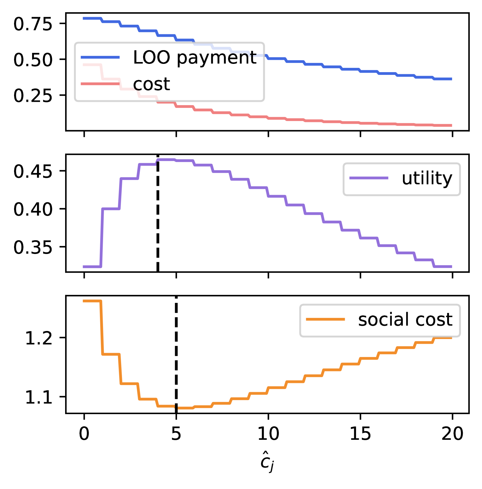
Existing data valuation methods for machine learning primarily focus on interpretability and guiding data collection, often neglecting market dynamics. In a market scenario, data owners (sellers) can misreport data-related costs to maximize their compensation, while data buyers strive to improve model performance at minimal cost. When valuation methods such as Leave-One-Out (Weisberg & Cook, 1982) and Data Shapley (Ghorbani & Zou, 2019) are directly used as pricing rules in data markets, we point out that data sellers are incentivized to misreport their true costs, resulting in inefficient data market collaboration. Even in the simplest mean estimation market, rational data owners are incentivized to misreport their costs, leading to suboptimal market efficiency, as illustrated in Figure 1.
To address the challenge of untruthful reporting, we draw on well-established payment mechanisms from game theory—specifically, the Myerson payment rule (Myerson, 1981) and the Vickrey–Clarke–Groves (VCG) mechanism (Vickrey, 1961; Clarke, 1971; Groves, 1973)—and adapt them to our data trading framework. Our analysis shows that: (1) the Myerson payment rule yields the minimum possible payment, making it optimal from the buyer’s standpoint; and (2) when allocations are made to maximize overall market welfare in an unconstrained setting, the VCG and Myerson payments coincide. Additionally, we demonstrate that when buyers’ utility functions are subadditive, total payments can be distributed across buyers while maintaining individual rationality for all participants. These findings highlight the crucial role of game-theoretic principles in designing data market payment schemes.
2 Related Work
Data Valuation Methods.
Data valuation has gained growing popularity in machine learning applications, mainly for the purposes of explainability and addressing algorithmic fairness (Pruthi et al., 2020; Liang et al., 2022), guiding high-quality data selection (Chhabra et al., 2024; Yu et al., 2024). Among them there are two primary categories methods – Shapley value based and Leave-One-Out (LOO) based. Shapley value based methods include Data Shapley (Ghorbani & Zou, 2019) and computationally feasible variations (Jia et al., 2020; Wang et al., 2024). LOO-based methods often encompass model retraining with one sample left out (Koh & Liang, 2020). In reality, rational participants in a market setting are likely to act strategically to maximize their profits. As a result, applying these pricing methods can lead to misreporting and inefficiencies within data markets.
Auction Theory and Mechanism Design.
Starting from the Arrow–Debreu model (Arrow & Debreu, 1954), a central question of market design is to set prices such that the net welfare of all participants is maximized. Such a market is said to be efficient. Auction theory (Krishna, 2003), and in general mechanism design, investigates how to how to design prices which preserve efficiency even if some information is unknown i.e. private. In the context of data markets, this implies that we want to design prices such that all participants truthfully report their true costs of data sharing and benefits received from said data, so that we can maximize social welfare.
Data Markets.
Due to unknown data sharing costs incurred by the data sellers, designing an efficient mechanism can be challenging. Dütting et al. (2021) show that with one data sample from the seller’s distribution, truthful mechanisms can be achieved with approximate market efficiency, assuming unit supply sellers. Rasouli & Jordarn (2021) design a truthful mechanism where data quality can be exchanged with monetary payments. However, they do not analyze its social efficiency. Agarwal et al. (2024) study truthful mechanism design when buyers’ externalities due to competition are known, aiming at maximizing social welfare or revenue. We refer to a recent survey (Zhang et al., 2024) for a more detailed overview of the area. We note that most of these works often assume known simple structured valuation functions and combinatorial allocations, not suitable for machine learning worlds where the information sharing can happen in continuous space and the buyers’ valuations are directly connected to model performances, which is our focus.
3 Problem Definition
3.1 Modeling Framework
We consider a data market with disjoint sets of data buyers and data sellers . . Buyers and seller interact through , where denotes the information exchange between buyer and seller . Depending on the use case, can live in different domains, which we will make it explicit in the use cases below.
Buyer’s Performance:
Each buyer has its performance (e.g. accuracy) function . The performance measures how buyer ’s model gets improved utilizing the data from the sellers. In the machine learning realm, is usually defined as the drop in validation loss after data is acquired, that is , where denotes the standalone loss for buyer . In game theory literature, such a performance function can as well be called buyer’s valuation.
Seller’s Cost:
The data sharing cost for seller is defined as , which is determined by how much information it has shared (i.e. ). is the seller-specific cost factor and quantifies the data sharing magnitude. For example, owners with expert-curated scientific data can have a higher than owners with synthetic data. is non-decreasing in the norm111can be any norm depending on the choice of data sellers of . The notion of data sharing cost can encompass data generation costs, costs due to privacy leakage, and etc. Using game theory terminology, the seller’s valuation is .
Assumption 1.
All and are differentiable with respect to .
Mechanism:
A mechanism is defined as , where is the allocation. determines the information exchange between buyers and sellers. specifies the payment each player receives or contributes. We assume such a payment rule is specified at the beginning of the game, that is, no re-distribution of payment is possible after the decision process. Further, denotes the price demanded from buyer and denotes the payment made to a seller .
Use Cases:
We list use cases where both buyers’ performance function and sellers’ data sharing costs can be modeled by .
-
i)
Acquiring Data from Multiple Domains: When conducting pre-training runs for LLMs, it is usually needed to decide on the data mixtures from different domains/sellers. With a larger , buyer benefits from more data from seller , and for seller , the costs for collecting and preparing the data also increase.
-
ii)
Model Sharing Markets: When sharing models, seller can (depedning on the price) choose to share an earlier checkpoint, or a smaller version of the model (e.g. 7B parameter version instead of the 70B version). The better seller ’s model is trained or larger is the model which is shared, the greater the data leakage is.
-
iii)
Differential Private Model Sharing: When sharing models, seller shares a noisy version of local model () with buyer , where . As increases, less noise is added to the model shared by seller , resulting in a higher degree of privacy leakage for seller . )
3.2 Definitions
We first give the following definitions, which are essential to guarantee the feasibility of the mechanism.
Definition 1 (Social Welfare and Social Cost).
Social welfare (SW) is the sum of all players’ valuations (buyers’ performance minus sellers’ costs)
Correspondingly, we can define social cost (SC), minimizing which is equivalent to maximizing the social welfare.
Definition 2 (Social Efficiency).
Collaboration denoted by is socially efficient (SE) if it minimizes the social cost or maximizes the social welfare.
Definition 3 (Individual Rationality).
Let be the price for the buyer and be the payment made to a seller . Then, we satisfy individual Rationality (IR) if
Intuitively, IR requires that the participants be better off participating in our mechanism than not.
Definition 4 (Incentive Compatibility or Truthful).
A mechanism is considered incentive-compatible (IC) if each participant achieves their best outcome by truthfully reporting their private values, regardless of what others report. We also refer to an IC mechanism as a truthful mechanism.
Definition 5 (Budget Balance).
A mechanism is called strong budget-balanced (SBB) if and weak budget-balanced (WBB) if .
4 Data Trading with Known Buyer Performance Function
In this section, we assume that only the seller side has private types, that are their cost factor , while the buyers’ performance functions are publicly known. We demonstrate that even in this simplified one-sided market, standard data valuation methods can incentivize sellers to misreport their information. To address this, we analyze existing truthful payment rules and characterize them in a data market scenario.
4.1 Problem Setup
Let be the reported costs from the sellers, we have allocation decided by the market platform dependent on the reported costs:
Due to this specific assignment function, it is clear that as long as sellers report their true costs , we have social efficiency achieved. We abuse the notation a bit, by letting both represent the allocation rule and the allocation itself.
Claim 1.
monotonically non-increasing in .
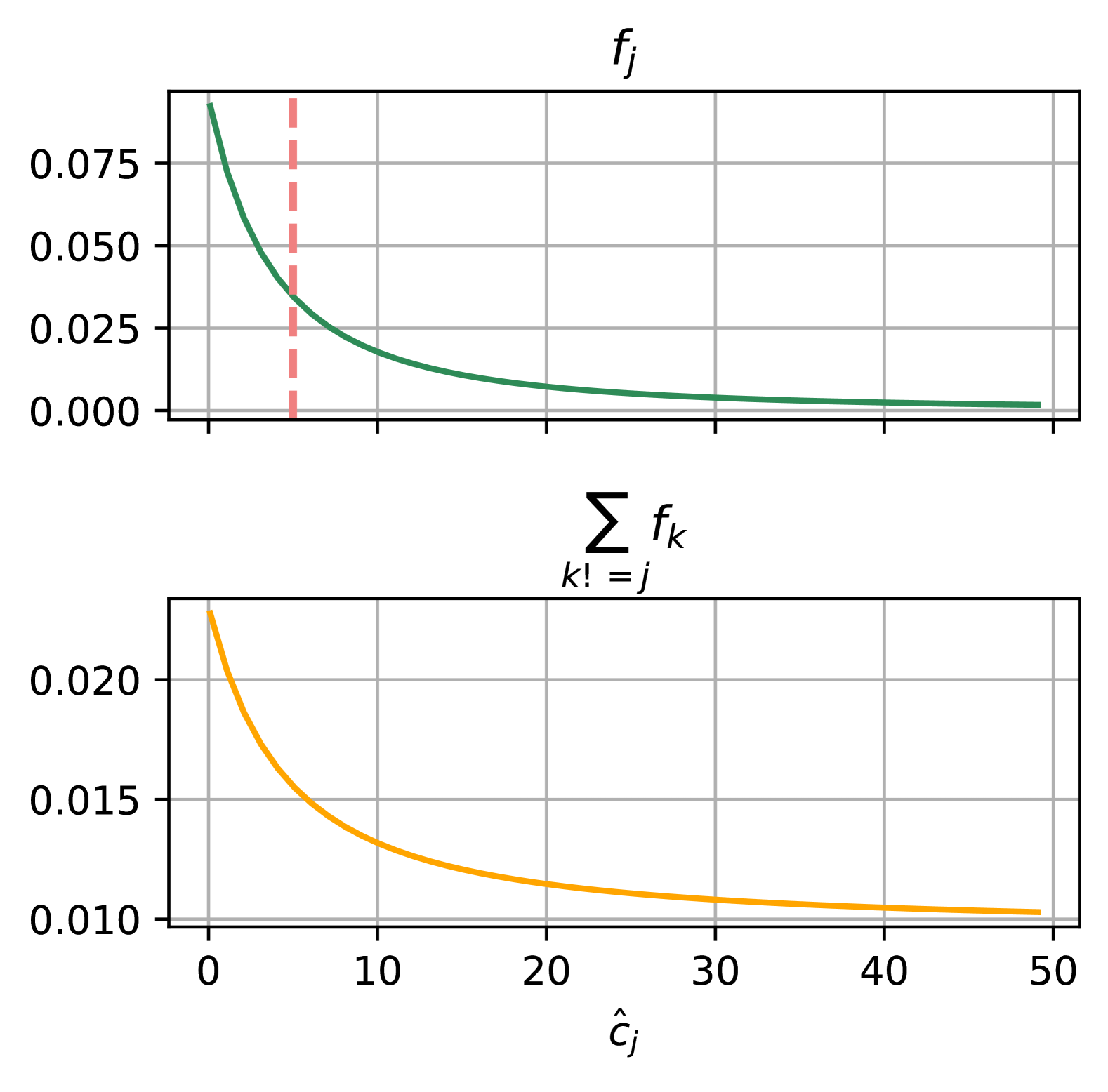
Proof can be seen in Appendix A.1.1. Claim 1 essentially states that seller ’s allocation gets smaller with a larger reported cost. At the same time, the total allocation to other sellers than (denoted by ) can increase or decrease in , as can have both positive and negative entries. We show this empirically in Figure 2.
4.2 Standard Data Valuation Methods
We begin by reviewing two conventional data valuation methods: Leave-One-Out valuation (Weisberg & Cook, 1982; Koh & Liang, 2020) and Data Shapley (Ghorbani & Zou, 2019). When seller compensation is based on these methods, we demonstrate that sellers are consistently incentivized to misreport their private types, as compensation depends on their self-reported information.
4.2.1 Leave-One-Out Payment Rule
Leave-one-out method (LOO) has been a standard approach to estimate influence in statistics (Weisberg & Cook, 1982; Koh & Liang, 2020). LOO valuation quantifies a data point’s contribution by assessing the change in model performance when the point is removed. This method inherently requires retraining the model on the reduced dataset. In our context, it corresponds to the following equation, representing the difference in buyers’ performance function with and without the presence of data seller .
| (1) |
Claim 2.
Using LOO valuation as the payment rule leads sellers to mis-report their true costs.
Proof.
For seller , the utility is
| (2) | ||||
Assume lies in an unconstrained domain. As is chosen by the system to maximize the reported social welfare, we have
| (3) |
Now we check how utility changes with respect to . In order to have optimality (), seller will report . To see this,
| (4) | ||||
| (5) | ||||
| (6) | ||||
| (7) |
We know , as the allocation to other buyers will change with . In order to have optimality, we would have . ∎
4.2.2 Payment via Shapley Value
Shapley value was first introduced to attribute fair contributions in a cooperative game by Shapley (1951). In the Machine Learning world, Data shapley (Ghorbani & Zou, 2019) was proposed to address data valuation. We adopt data shapley calculation in our scenario, as in (8). The idea is to calculate the marginal contribution of seller , averaged over all subsets of sellers. Depending on the market size, the calculation of Shapley value can be computationally inefficient. In contrast, LOO payment only considers the marginal contribution to the subset .
| (8) |
is calculated from where
Remark 1.
is not IC either. As like LOO payment, the utility of seller is dependent on its reported , and thus a rational seller can manipulate to arrive at a higher utility.
Remark 2.
If the performance function is super-additive222 specified by are super-additive in the set of data sellers (e.g. when complementary but necessary data sources are combined to solve a task), LOO payment is greater than Shapley payment. On the flip side, if the performance function is sub-additive333 specified by are sub-additive in the set of data sellers (e.g. when the contribution of one user is very similar to that of another), LOO payment is smaller than Shapley payment.
4.3 Examing Existing Truthful Payment Rules
Since popular data valuation strategies can perform arbitrarily poorly with respect to truthfulness, we turn to established theoretical results that guarantee truthful payments. We show that the Myerson payment rule yields the minimal payment necessary to ensure truthfulness, making it optimal from the buyer’s perspective. Moreover, when the choice of allocation rule is unconstrained, we demonstrate an equivalence between the VCG and Myerson payment rules.
4.3.1 Myerson payment rule
Myerson payment is a classical truthful payment rule (Myerson, 1981), which pays sellers the reported cost plus an integral term. Our specific scenario maps to the following equation in (9). It guarantees truthful reporting as long as is monotonically non-increasing in , which we prove in Claim 1.
| (9) |
Claim 3.
The Myerson payment rule is IC and IR for all buyers.
Proof.
We can write down the utility of seller
is maximized at , and is always greater than since . ∎
4.3.2 VCG payment rule
Vickrey–Clarke–Groves (VCG) payment (Vickrey, 1961; Clarke, 1971; Groves, 1973) is another classical payment rule, which calculates the externality of a specific seller to the social welfare, as in (10). The idea is to calculate the differences between the social welfare of in seller ’s absence and the welfare when seller is present.
| (10) | ||||
Claim 4.
VCG payment rule is IC and IR for all sellers.
Proof.
is IC by design. To see the IR part, we check the utility for any seller :
∎
Claim 5.
, where is with the th column set to zero, and all other entries unchanged.
4.4 Characterization of the truthful payment rules
Myerson and VCG payment rules are both IC, seller-IR and socially optimal. How do they compare to each other? Theorem 4.1 shows that in general, Myerson is the smallest payment rule, thus optimal from the buyers’ perspective. In certain scenarios, i.e. when lives in an unconstrained domain, we further have VCG payment equivalent to Myerson payment, which is proven in Theorem 4.2.
Theorem 4.1.
Myerson payment is the smallest IC and IR (for data sellers) payment rule.
Proof can be checked at Appendix A.1.2.
Theorem 4.2.
Myerson payment is equivalent to the VCG payment when is chosen to maximize social welfare and when the domain of is unconstrained.
Proof.
Keep other sellers’ reported fixed, we have social welfare as a function of seller ’ reported
| (12) |
As is chosen by the system to maximize the reported social welfare, we have
| (13) |
We further show that
| (14) | ||||
Thus, we can calculate the integral part of the Myerson payment as
| (15) |
As Myerson payment will incentivizes truthful reporting, we have
| (16) | ||||
∎
Discussion. Myerson payment rule provides theoretical guarantees of being buyer-optimal. However, its computation can be costly since requires optimizing , the complexity of which depends on the structure of and . VCG payment, on the other hand, is more computationally feasible. Yet, it still requires leave-one-out retraining. Future work should explore more computationally efficient implementations.
4.5 IR for data buyers?
Until now, we have focused solely on the seller side. But can our mechanism also benefit data buyers? Interestingly, we can redistribute the payments made to sellers among buyers based on their marginal contributions. This ensures SBB in the market and guarantees IR for data buyers when the performance function is subadditive.
Theorem 4.3.
Assume is subadditive (i.e. has diminishing returns in ). A payment rule defined as follows is IR for all buyers.
| (17) |
Proof.
As is the minimal payment rule that fulfills IC and IR for sellers, we must have . Claim 5 indicates
| (18) |
Following the choice of , we have
| (19) |
We can thus bound the payment from buyer by
| (20) |
The final inequality is a consequence of the sub-additivity assumption, under which the aggregate contribution of data sellers is bounded above by the sum of their separate contributions. ∎
Remark 3.
When the performance function is super-additive, we currently lack a solution that guarantees individual rationality (IR) for the buyer. Whether it is possible to design a suitable buyer payment mechanism remains an open question.
5 Challenges with Private Buyer Performance
So far, we have looked into the scenario where buyers’ performance function is assumed to be known. In practice, such functions are usually private, especially when entering into a new market with no historical records. Or when sharing the performance functions violates the buyer’s privacy. In such cases, we show that it is impossible to design any payment rule that simultaneously achieves IC, IR, WBB, and SE. In fact, the social cost may be arbitrarily far from the efficient solution. This result is similar in spirit to the celebrated Myerson–Satterthwaite theorem (Myerson & Satterthwaite, 1983) proving the impossibility of efficient bilateral trade (double auctions). The negative results open up a new challenge for designing valuation and pricing rules for data markets.
5.1 An Impossibility Result
Theorem 5.1 (cr. Holmström (1979)).
Assume all participants’ valuation . If is a convex domain, then Groves mechanism that is defined by the allocation rule
and payment rule
is the unique IC mechanism, up to the choice of
Theorem 5.2 (Impossibility Result).
When buyers and sellers both have their private types to report, no single mechanism can simultaneously satisfy IR, WBB, IC and SE. Further, any mechanism that ensures WBB, IR, and IC can result in arbitrarily poor social efficiency.
Proof can be checked at Appendix A.1.3.
6 Experiments and Simulations
In this section, we illustrate our modeling framework with a simple mean estimation game and a more realistic data mixture game. We empirically demonstrate that directly applying LOO and Shapley Value-based valuation as pricing rules results in untruthful reporting.
6.1 Mean Estimation Markets
In this example, we consider disjoint sets of buyers and sellers . Choose and . The buyers try to estimate their local means . Sellers have local estimates from their own local samples sampled from , . In order to achieve lower MSE loss, users may seek trading with each other for their local estimates. We choose to be , where is decided as the minimizer of the reported social cost.
| (21) |
Due to the unique quadratic structure of the objective, we have a closed-form solution of in (22). The proof is provided in Appendix A.1.4.
| (22) |
where , , and
6.1.1 Comparison of different truthful payment rules
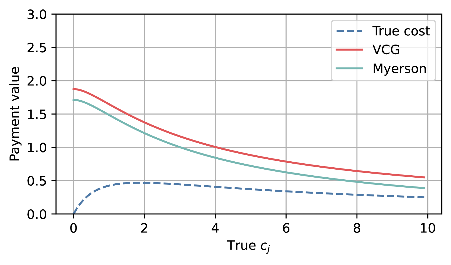
We focus on the seller with index and analyze its payment and cost while keeping the reported costs of other sellers fixed. This allows us to easily compute and compare different payment rules as we vary the true . In the mean estimation market, can have negative entries. Thus, can decrease or increase with , while always decrease with . This is shown in Figure 2, where the results of two randomly generated mean estimation markets are presented. Since lies in an unconstrained domain, we have VCG payment equivalent to Myerson payment, as shown in Figure 3(a), where the value mismatch is due to numerical issues.


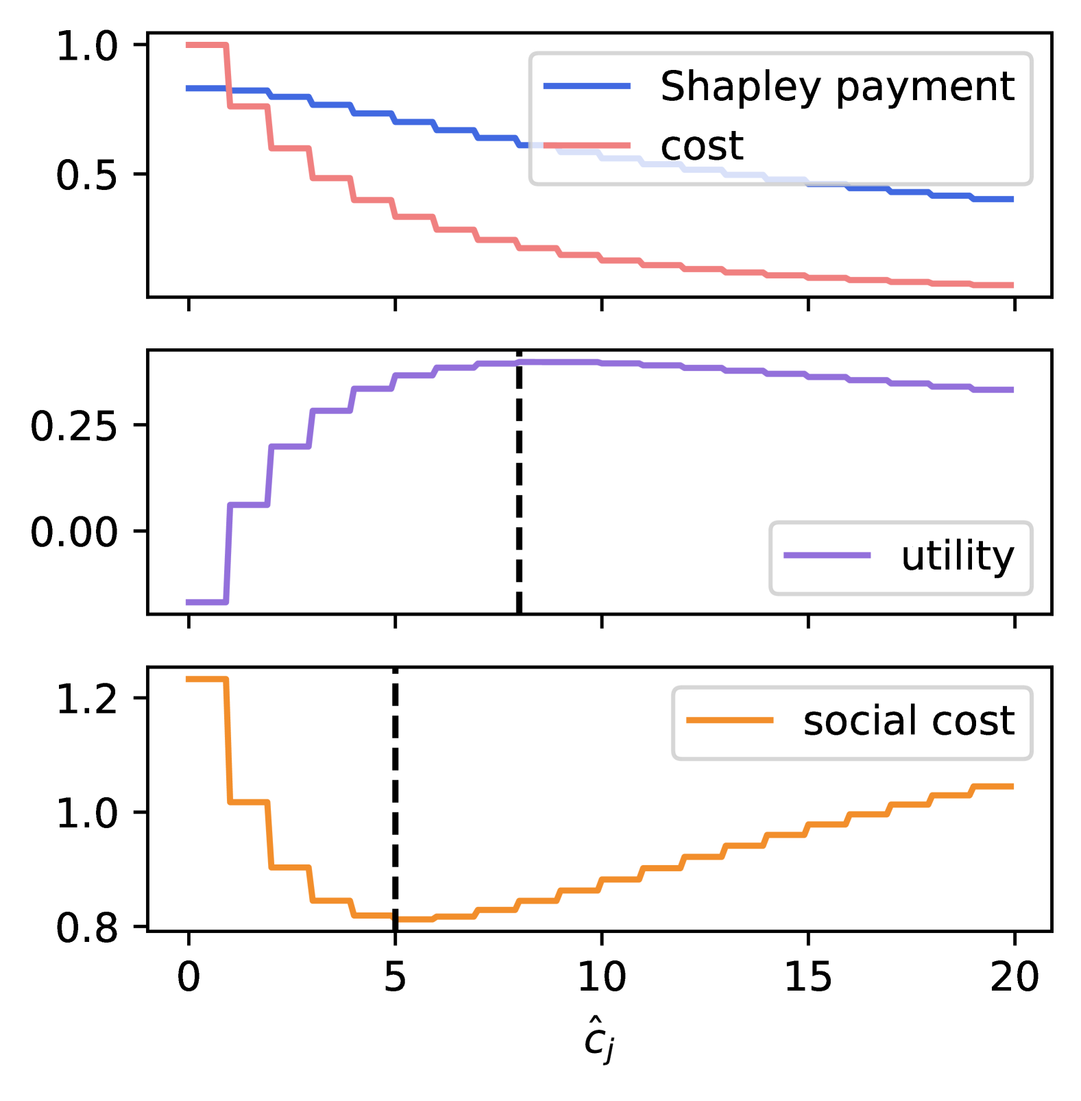
6.1.2 Mis-reporting for Untruthful payment rules
Let true . We compute the payment values and resulted utility when varying the reported . Given our choice of , social cost is always minimized at . However, with LOO and Shapley payment rule, the resulted utilities peak at a different value than , as shown in Figure 1.
LOO Payment Rule.
To maximize its utility, seller will mis-report . The resulting .
Shapley Payment Rule.
To maximize its utility, seller will mis-report . The resulting
6.2 Data Mixture Market
Our framework extends to LLM training as well. For simplicity, we consider a single buyer that is seeking for purchasing data from different data sellers to arrive at a good pretrained model. From Ye et al. (2024), the relationship between proportions of data mixtures and the validation loss in the target domain can be modeled via (23), assuming fixed token budgets. and are constant scalars, and captures the how the training data of seller helps reduce validation loss on the target domain. denotes the proportion of pertaining data from each seller .
| (23) |
Following our framework, the data mixtures can be determined from minimizing the social cost objective in (24).
| (24) |
In practice, (23) can be estimated using a small LM on small datasets. To pre-determine the data mixtures via a smaller LM is a standard practice in LLM pre-training. Here we randomly sample some values to be . Given that here are row-stochastic, the rank of truthful payment methods again confirms our theoretical analysis, as shown in Figure 3(b).
7 Conclusion
Our work serves as a first step in bridging the gap between theoretical results in incentive compatible mechanism design and more empirically driven data valuation methods in machine learning. We demonstrate that standard data valuation methods, such as Leave-One-Out and Data Shapley, fail to incentivize truthful reporting in a data market with private information. Myerson payment is buyer-optimal while being incentive-compatible and individual-rational. We also show that when both buyer and seller information is private, we have unbounded price of anarchy in general.
Our findings open several directions for future work: 1) how to make the existent truthful payment rule more computationally efficient? 2) in settings where both buyers and sellers have private valuations, can we impose some structural assumptions on their valuations and costs to establish approximation guarantees similar in spirit to McAffee’s trade reduction mechanism (McAfee, 1992)? Taken together, we hope our work initiates an important and fruitful line of research in designing practical pricing strategies with game-theoretic considerations in realistic data markets.
Acknowledgement. We thank Neel Patel for helpful discussions throughout the project and anonymous reviewers for their constructive feedback.
References
- Agarwal et al. (2024) Anish Agarwal, Munther Dahleh, Thibaut Horel, and Maryann Rui. Towards data auctions with externalities. Games and Economic Behavior, 148:323–356, November 2024. ISSN 0899-8256. doi: 10.1016/j.geb.2024.09.008. URL http://dx.doi.org/10.1016/j.geb.2024.09.008.
- Arrow & Debreu (1954) Kenneth J Arrow and Gerard Debreu. Existence of an equilibrium for a competitive economy. Econometrica: Journal of the Econometric Society, pp. 265–290, 1954.
- Chhabra et al. (2024) Anshuman Chhabra, Peizhao Li, Prasant Mohapatra, and Hongfu Liu. ” what data benefits my classifier?” enhancing model performance and interpretability through influence-based data selection. In The Twelfth International Conference on Learning Representations, 2024.
- Clarke (1971) Edward H. Clarke. Multipart pricing of public goods. Public Choice, 1971.
- Concord Music Group v. Anthropic (2023) Concord Music Group v. Anthropic. Case no. 3:23-cv-01092, m.d. tenn., nashville div. https://caselaw.findlaw.com/court/us-dis-crt-m-d-ten-nas-div/116305682.html, 2023. U.S. District Court.
- Dütting et al. (2021) Paul Dütting, Federico Fusco, Philip Lazos, Stefano Leonardi, and Rebecca Reiffenhäuser. Efficient two-sided markets with limited information. In Proceedings of the 53rd Annual ACM SIGACT Symposium on Theory of Computing, STOC ’21, pp. 1452–1465. ACM, June 2021. doi: 10.1145/3406325.3451076. URL http://dx.doi.org/10.1145/3406325.3451076.
- Ghorbani & Zou (2019) Amirata Ghorbani and James Zou. Data shapley: Equitable valuation of data for machine learning. In International Conference on Machine Learning, pp. 2242–2251, 2019.
- Groves (1973) Theodore Groves. Incentives in teams. Econometrica, 1973.
- Holmström (1979) Bengt Holmström. Groves’ scheme on restricted domains. Econometrica: Journal of the Econometric Society, pp. 1137–1144, 1979.
- Jia et al. (2020) Ruoxi Jia, David Dao, Boxin Wang, Frances Ann Hubis, Nezihe Merve Gurel, Bo Li, Ce Zhang, Costas J. Spanos, and Dawn Song. Efficient task-specific data valuation for nearest neighbor algorithms, 2020. URL https://arxiv.org/abs/1908.08619.
- Koh & Liang (2020) Pang Wei Koh and Percy Liang. Understanding black-box predictions via influence functions, 2020. URL https://arxiv.org/abs/1703.04730.
- Krishna (2003) Vijay Krishna. Auction Theory. Elsevier Inc., United States, 2003. ISBN 9780124262973. doi: 10.1016/B978-0-12-426297-3.X5026-7.
- Liang et al. (2022) Weixin Liang, Girmaw Abebe Tadesse, Daniel Ho, Li Fei-Fei, Matei Zaharia, Ce Zhang, and James Zou. Advances, challenges and opportunities in creating data for trustworthy ai. Nature Machine Intelligence, 4(8):669–677, 2022.
- Longpre et al. (2023) Shayne Longpre, Robert Mahari, Anthony Chen, Naana Obeng-Marnu, Damien Sileo, William Brannon, Niklas Muennighoff, Nathan Khazam, Jad Kabbara, Kartik Perisetla, Xinyi Wu, Enrico Shippole, Kurt Bollacker, Tongshuang Wu, Luis Villa, Sandy Pentland, and Sara Hooker. The data provenance initiative: A large scale audit of dataset licensing & attribution in ai, 2023. URL https://arxiv.org/abs/2310.16787.
- Longpre et al. (2024) Shayne Longpre, Robert Mahari, Ariel Lee, Campbell Lund, Hamidah Oderinwale, William Brannon, Nayan Saxena, Naana Obeng-Marnu, Tobin South, Cole Hunter, Kevin Klyman, Christopher Klamm, Hailey Schoelkopf, Nikhil Singh, Manuel Cherep, Ahmad Anis, An Dinh, Caroline Chitongo, Da Yin, Damien Sileo, Deividas Mataciunas, Diganta Misra, Emad Alghamdi, Enrico Shippole, Jianguo Zhang, Joanna Materzynska, Kun Qian, Kush Tiwary, Lester Miranda, Manan Dey, Minnie Liang, Mohammed Hamdy, Niklas Muennighoff, Seonghyeon Ye, Seungone Kim, Shrestha Mohanty, Vipul Gupta, Vivek Sharma, Vu Minh Chien, Xuhui Zhou, Yizhi Li, Caiming Xiong, Luis Villa, Stella Biderman, Hanlin Li, Daphne Ippolito, Sara Hooker, Jad Kabbara, and Sandy Pentland. Consent in crisis: The rapid decline of the ai data commons, 2024. URL https://arxiv.org/abs/2407.14933.
- McAfee (1992) R Preston McAfee. A dominant strategy double auction. Journal of economic Theory, 56(2):434–450, 1992.
- Myerson (1981) Roger B. Myerson. Optimal auction design. Mathematics of Operations Research, 1981.
- Myerson & Satterthwaite (1983) Roger B Myerson and Mark A Satterthwaite. Efficient mechanisms for bilateral trading. Journal of economic theory, 29(2):265–281, 1983.
- New York Times v. OpenAI (2023) New York Times v. OpenAI. Case no. 1:23-cv-11195, s.d.n.y. https://nytco-assets.nytimes.com/2023/12/NYT_Complaint_Dec2023.pdf, 2023. U.S. District Court for the Southern District of New York.
- Pruthi et al. (2020) Garima Pruthi, Frederick Liu, Satyen Kale, and Mukund Sundararajan. Estimating training data influence by tracing gradient descent. In H. Larochelle, M. Ranzato, R. Hadsell, M.F. Balcan, and H. Lin (eds.), Advances in Neural Information Processing Systems, volume 33, pp. 19920–19930. Curran Associates, Inc., 2020. URL https://proceedings.neurips.cc/paper_files/paper/2020/file/e6385d39ec9394f2f3a354d9d2b88eec-Paper.pdf.
- Rasouli & Jordarn (2021) Mohammad Rasouli and Michael I. Jordarn. Data sharing markets, 2021. URL https://arxiv.org/abs/2107.08630.
- Shapley (1951) Lloyd S. Shapley. Notes on the N-Person Game — II: The Value of an N-Person Game. RAND Corporation, Santa Monica, CA, 1951. doi: 10.7249/RM0670.
- Vickrey (1961) William Vickrey. Counterspeculation, auctions, and competitive sealed tenders. Journal of Finance, 1961.
- Villalobos et al. (2024) Pablo Villalobos, Anson Ho, Jaime Sevilla, Tamay Besiroglu, Lennart Heim, and Marius Hobbhahn. Will we run out of data? limits of llm scaling based on human-generated data, 2024. URL https://arxiv.org/abs/2211.04325.
- Wang et al. (2024) Jiachen T Wang, Prateek Mittal, Dawn Song, and Ruoxi Jia. Data shapley in one training run. arXiv preprint arXiv:2406.11011, 2024.
- Weisberg & Cook (1982) Sanford Weisberg and R Dennis Cook. Residuals and influence in regression. 1982.
- Ye et al. (2024) Jiasheng Ye, Peiju Liu, Tianxiang Sun, Yunhua Zhou, Jun Zhan, and Xipeng Qiu. Data mixing laws: Optimizing data mixtures by predicting language modeling performance, 2024. URL https://arxiv.org/abs/2403.16952.
- Yu et al. (2024) Zichun Yu, Spandan Das, and Chenyan Xiong. Mates: Model-aware data selection for efficient pretraining with data influence models. arXiv preprint arXiv:2406.06046, 2024.
- Zhang et al. (2024) Jiayao Zhang, Yuran Bi, Mengye Cheng, Jinfei Liu, Kui Ren, Qiheng Sun, Yihang Wu, Yang Cao, Raul Castro Fernandez, Haifeng Xu, et al. A survey on data markets. arXiv preprint arXiv:2411.07267, 2024.
Appendix A Appendix
A.1 Missing Proofs
A.1.1 Proof for Claim 1
is chosen to optimize the following function according to our setup
Suppose for contradiction, there exist two reported costs such that:
By optimality of the allocation , we have that:
| (25) | ||||
and similarly,
| (26) | ||||
Adding these two inequalities together, we find:
Since by assumption , it must be the case that:
contradicting our initial assumption. Therefore, the function is monotonically non-increasing in the seller’s reported cost
A.1.2 Proof for Theorem 4.1
Proof.
From the IC condition, we have
| (27) |
| (28) |
| (29) |
Let , and , with , we have
| (30) |
and thus
| (31) |
We have
| (32) | ||||
Constrained to IR, we have . Myerson payment is when is chosen as . ∎
A.1.3 Proof for Theorem 5.2
We consider a simple one-buyer-one-seller case, where the reported valuations are
| (33) |
where . Truthfulness requires Groves payment rule, thus and . With truthful reporting, we have social efficiency directly follows as the coordinator chooses socially optimal .
Now we check IR and WBB conditions, with IR, we have
| (34) |
With WBB, we have
| (35) |
Let , we have . This implies . Analogously, .
Let and , we have and . Plugging in (35), we have
which suggests . It can only be . That is, . Both the buyer and the seller only take their own valuations into account. As the seller’s valuation will be negative as long as , constrained to IR conditions, there will not be trade happening.
Now let’s check the Price of Anarchy (PoA):
| (36) |
PoA can be arbitrarily large if , when happens when seller has exactly the data buyer needs, which makes buyer ’s loss goes to 0, and the cost is 0.
A.1.4 Derivation of W in Mean Estimation Market
We offer the proof for the derivation of closed-form in Section 6.1.
| (37) |
| (38) | ||||
We have
Thus,
A.2 Additional Experimental Results
A.2.1 LOO payment vs. Shapley payment
Using LOO or Shapley can lead to over-report or under-report, as illustrated in Figure 4.