M²IV: Towards Efficient and Fine-grained Multimodal In-Context Learning in Large Vision-Language Models

Abstract

Multimodal in-context learning (ICL) is a vital capability for Large Vision-Language Models (LVLMs), allowing task adaptation via contextual prompts without parameter retraining. However, its application is hindered by the token-intensive nature of inputs and the high complexity of cross-modal few-shot learning, which limits the expressive power of representation methods. To tackle these challenges, we propose M²IV, a method that substitutes explicit demonstrations with learnable In-context Vectors directly integrated into LVLMs. By exploiting the complementary strengths of multi-head attention (MHA) and multi-layer perceptrons (MLP), M²IV achieves robust cross-modal fidelity and fine-grained semantic distillation through training. This significantly enhances performance across diverse LVLMs and tasks and scales efficiently to many-shot scenarios, bypassing the context window limitations. We also introduce VLibrary, a repository for storing and retrieving M²IV, enabling flexible LVLM steering for tasks like cross-modal alignment, customized generation and safety improvement. Experiments across seven benchmarks and three LVLMs show that M²IV surpasses Vanilla ICL and prior representation engineering approaches, with an average accuracy gain of 3.74% over ICL with the same shot count, alongside substantial efficiency advantages.

1 Introduction

Large Vision-Language Models (LVLMs) integrate visual and textual modalities by aligning their embedding spaces, enabling advanced multimodal understanding and generation capabilities powered by Large Language Models (LLMs) (Zhou et al., 2022; Zhang et al., 2024; Laurençon et al., 2025). LVLMs have been successfully applied across a wide spectrum of Vision-Language (VL) tasks (Hartsock & Rasool, 2024; Xu et al., 2024). Given the growing complexity of tasks, the efficient utilization of LVLMs is increasingly crucial. In-context learning (ICL) presents a compelling solution that facilitates rapid adaptation to novel tasks without the need for extensive parameter updates (Brown et al., 2020; Dong et al., 2022).

While progress has been made in applying multimodal ICL to tasks such as image captioning and classification (Yang et al., 2023; Huang et al., 2024), extending this paradigm to more complex or knowledge-intensive scenarios remains a significant challenge (Li et al., 2024). Two core conflicts underlie this difficulty. First, there is a trade-off between the need for knowledge integration and the token-heavy nature of multimodal inputs (Chevalier et al., 2023; Huang et al., 2025). Given the limited context window of LVLMs, knowledge augmentation strategies (Xia et al., 2024) often require splitting inputs into multiple turns, increasing the risk of catastrophic forgetting (He et al., 2024). In addition, larger input volumes significantly reduce inference efficiency. Second, there exists an inherent instability in few-shot learning. Despite the benefits of scaling models, LVLMs remain highly sensitive to prompt format and ordering (Ye & Durrett, 2022), with even state-of-the-art models experiencing notable performance drops under few-shot settings (DeepSeek-AI et al., 2025). This issue is exacerbated in multimodal contexts (Lu et al., 2021; Qin et al., 2025).

In response to these challenges, representation engineering has emerged as a promising alternative. This approach leverages the findings that ICL prompts modulate internal activations (Merullo et al., 2023), enabling the extraction of intermediate representations which can then be reinjected during zero-shot inference to encode task-specific guidance. For instance, Hendel et al. (2023) derive task vectors from the hidden state of the context’s final token, while Todd et al. (2024) compute function vectors by averaging the outputs of key attention heads. Although these methods perform well on simpler tasks with straightforward mappings, they struggle with multimodal tasks like VQA. Consequently, Peng et al. (2025) propose training in-context vectors to capture richer features for multimodal expansion; however, their approach still suffers from rapid degradation as complexity increases. This indicates a shared limitation: an inability to effectively model intricate cross-modal interactions. To overcome this shortcoming in multimodal ICL, two key challenges must be tackled simultaneously: ① identifying the critical task mappings within individual demonstrations and the interdependencies among different demonstrations, and ② achieving fine-grained semantic distillation of this multifaceted information.

Building on these insights, we introduce M²IV, a novel method that harnesses the distinct roles of multi-head attention (MHA) and multi-layer perceptrons (MLP) in multimodal ICL. To ensure that these vectors effectively capture the deep semantic patterns in demonstrations, as processed by the MHA, and simulate the detailed distillation of complex information executed by the MLP, we devise a specialized training strategy. The experiments show that M2IV achieved SOTA performance in 18 out of 21 experiments conducted on three LVLMs and seven benchmarks, while utilizing only about 24% of the total training data employed by LIVE. Furthermore, M²IV embodies a breakthrough in efficiency as its improvements in inference time completely offset the training cost and promise even higher cost effectiveness when widely adopted. To further explore the potential of M²IV, we present VLibrary, a container for storing and retrieving M²IV representations that facilitates efficient and ready integration. VLibrary can be seamlessly incorporated into real-world systems and applied to address critical challenges in the LVLM domain.

Our main contributions are: (1) We analyze the unique roles of MHA and MLP in multimodal ICL, revealing how MHA drives semantic integration and MLP refines fine-grained details. (2) We propose M²IV, which simultaneously achieves complex semantic understanding and fine-grained semantic distillation, demonstrating superior performance across three LVLMs and seven diverse benchmarks. (3) We introduce VLibrary and use it to address three critical challenges: cross-modal alignment, output customization, and safety, thereby offering a novel and promising approach for future LVLM research.

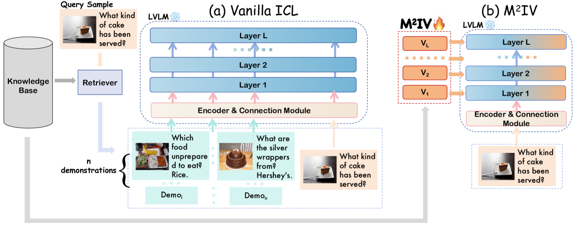
Figure 1: (a) In Vanilla ICL, for a given query sample, we retrieve $n$ instances from a knowledge base as demonstrations and feed them together with the query sample into the LVLM. (b) In contrast, we train a set of vectors emulating $n$-shot ICL using the same knowledge base and inject these vectors into the LVLM, greatly reducing token consumption and boosting model performance.

2 Background and Related Works

ICL emerges as a pivotal capability in large-scale LLMs (Radford et al., 2019; Garg et al., 2022) and has since been extended to the multimodal domain. Several LVLMs are specifically pretrained or fine-tuned to enable robust multimodal ICL, among the most notable are OpenFlamingo (Awadalla et al., 2023) and IDEFICS (Laurençon et al., 2024), which form key components of our work. As demand for multimodal ICL continues to rise, supporting it within fixed context windows has become an essential capability of general-purpose LVLMs, such as Qwen2.5VL (Bai et al., 2025) and Grok 3 (xAI, 2025).

In LVLMs, ICL is defined as the process in which a pretrained model $\mathcal{M}$ is provided with a prompt containing a multimodal context $\mathbf{C}$ (absent in zero-shot settings) and a query sample $\mathbf{Q}$. To generate the answer $\mathbf{A}$, the model computes the conditional probability:

$$P_{\mathcal{M}}\left(\mathbf{A}|\mathbf{Q},\mathbf{C}\right)$$ (1)

via a feed-forward pass. $\mathbf{C}$ includes few-shot demonstrations, as shown in Figure 1(a).

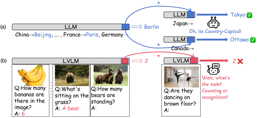
Figure 2: Overview of applying Function Vector to (a) the Country-Capital task and (b) the VQA task, which requires complex reasoning. While it performs well in (a), it falls short of fully representing the context in (b).

With the prevalence of ICL, researchers have been investigating its underlying mechanisms (Xie et al., 2021; Dai et al., 2023), They point out that key attention dynamics, most notably skill neurons and induction heads (Wang et al., 2022), play a crucial role in its success. These insights have driven advances in ICL representation engineering. Firstly, Hendel et al. (2023) and Todd et al. (2024) nearly simultaneously propose Task Vector (TV) and Function Vector (FV). Building on this, Liu et al. (2024c) obtain layer-wise In-Context Vectors (ICVs) by comparing the hidden states of the final tokens in the original and target sequences, then applying PCA to distill task-relevant information. Expanding this approach further, Li et al. (2025) propose Implicit ICL (I2CL), which extracts residual stream deltas at each demonstration’s last token position across layers and utilizes a set of coefficients to regulate their injection. As noted in §1 and illustrated in Figure 2, these methods often underperform in multimodal ICL. Peng et al. (2025) attribute this gap to the static extraction-injection paradigm and propose an attention shifting-based training method LIVE, yet their approach still neglects the essential role of fine-grained semantic distillation.

3 Methodology

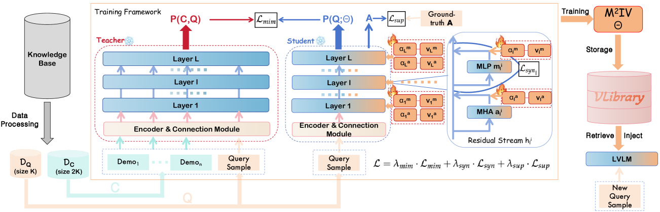
Figure 3: Pipeline of M²IV training and storage. We begin by constructing the training sets $\mathcal{D}_{\textbf{Q}}$ and $\mathcal{D}_{\textbf{C}}$. from an existing knowledge base. Next, a self-distillation framework employing three losses ($\mathcal{L}_{mim}$, $\mathcal{L}_{syn}$ and $\mathcal{L}_{sup}$) is used to train M²IV. Finally, the trained M²IV is stored in VLibrary for on-demand retrieval.

In this section, we detail the proposed M²IV framework. by analyzing the roles of MHA and MLP in LVLM ICL, which motivates our definition of the M²IV parameters (§3.1). We then present the complete training strategy (§3.2). Finally, we introduce VLibrary, the storage for M²IVs (§3.3). The overview pipeline is illustrated in Figure 3.

3.1 Anchoring M²IV

For an $L$-layer LVLM $\mathcal{M}$ processing an input sequence of length $I$, the residual stream architecture is recursively defined as follows, with $l\in\left\{1,2,\dots,L\right\}$ and $i\in\left\{1,2,\dots,I\right\}$:

$$\mathbf{a}_{l}^{i} =\text{MHA}\left(\mathbf{h}_{l-1}^{i};\theta_{l}\right),$$ (2)

$$\mathbf{m}_{l}^{i} =\text{MLP}\left(\mathbf{h}_{l-1}^{i}+\mathbf{a}_{l}^{i};W_{l}\right),$$ (3)

$$\mathbf{h}_{l}^{i} =\mathbf{h}_{l-1}^{i}+\mathbf{a}_{l}^{i}+\mathbf{m}_{l}^{i},$$ (4)

where $\mathbf{h}_{l}^{i}\in\mathbb{R}^{d_{\mathcal{M}}}$ denotes the residual stream at layer $l$ and position $i$, with hidden dimension $d_{\mathcal{M}}$. The functions $\text{MHA}\left(\cdot;\theta_{l}\right):\mathbb{R}^{d_{\mathcal{M}}}\to\mathbb{R}^{d_{\mathcal{M}}}$ and $\text{MLP}\left(\cdot;W_{l}\right):\mathbb{R}^{d_{\mathcal{M}}}\to\mathbb{R}^{d_{\mathcal{M}}}$ denote the MHA and MLP transformations at layer $l$, parameterized by $\theta_{l}$ and $W_{l}$, respectively.

Previous research (Chang et al., 2024; Li et al., 2025) has demonstrated that MHA and MLP branches play distinct roles in ICL. Based on these insights, we infer that in multimodal ICL, MHA dynamically allocates attention to capture both the internal semantics within demonstrations and the interactions among them. MLP further extracts, filters, and stores key information in a fine-grained manner, conveying more aggregated yet nuanced features. To validate our inferences, we explore their computational invariance for a demonstration matrix $\mathbf{C}\in\mathbb{R}^{C\times d_{\mathcal{M}}}$ with $C$ tokens, and two invariance properties are established.

Theorem 1.

(MHA Computational Invariance) There exists $\Psi:\mathbf{D}_{\Psi}\to\mathbb{R}^{d_{\mathcal{M}}}$ such that, for any query matrix $\mathbf{Q}\in\mathbb{R}^{I\times d_{\mathcal{M}}}$ and residual stream $\mathbf{h}^{i}\in\mathbb{R}^{d_{\mathcal{M}}}$, there exist $\zeta^{i}$, $\eta^{i}\in\mathbb{R}$ satisfying:

$$\mathrm{Attn}\left(\mathbf{h}^{i},\begin{bmatrix}\mathbf{C}^{\top}\>\mathbf{Q}^{\top}\end{bmatrix}^{\top},\begin{bmatrix}\mathbf{C}^{\top}\>\mathbf{Q}^{\top}\end{bmatrix}^{\top}\right)=\zeta^{i}\cdot\Psi\left(\mathbf{h}^{i},\mathbf{C},\mathbf{C}\right)+\eta^{i}\cdot\mathrm{Attn}\left(\mathbf{h}^{i},\mathbf{Q},\mathbf{Q}\right),$$ (5)

where $\mathrm{Attn}\left(\cdot\right)$ is a function representing the self-attention mechanism.

Remark. Theorem 1 shows that the self-attention mechanism decomposes into two parts: a query-only component, $\text{Attn}(\mathbf{h}^{i},\mathbf{Q},\mathbf{Q})$, and a context-augmented component, $\Psi(\mathbf{h}^{i},\mathbf{C},\mathbf{C})$. This decomposition highlights MHA’s role in dynamically allocating attention, allowing $\mathcal{M}$ to integrate query-specific focus with contextual insights from demonstrations in ICL.

Theorem 2.

(MLP Computational Invariance) For linear transformation matrix $W\in\mathbb{R}^{d_{\mathcal{M}}\times d_{\mathcal{M}}}$ , there exists $\psi_{W}:\mathbb{R}^{d_{\mathcal{M}}}\to\mathbb{R}^{d_{\mathcal{M}}}$ such that, for any token position $i$, there exist $\zeta^{i}$, $\eta^{i}\in\mathbb{R}$ satisfying:

$$\mathrm{MLP}\left(\mathbf{a}^{i}_{\mathbf{C},\mathbf{Q}}\right)=\zeta^{i}\cdot\psi_{W}\left(\mathbf{a}^{i}_{\mathbf{C}}\right)+\eta^{i}\cdot\mathrm{MLP}\left(\mathbf{a}^{i}_{\mathbf{Q}}\right),$$ (6)

where $\mathrm{MLP}\left(\cdot\right)$ represents the MLP mechanism, and $\mathbf{a}^{i}_{\mathbf{Q},\mathbf{C}}$, $\mathbf{a}^{i}_{\mathbf{Q}}$, and $\mathbf{a}^{i}_{\mathbf{C}}$ are the MHA outputs at the $i$-th token position with both query and context, with query-only, and with context-only, respectively.

Remark. Theorem 2 shows that the MLP mechanism decomposes into two parts: a query-only component, $\text{MLP}(\mathbf{a}^{i}_{\mathbf{Q}})$, and a context-enhanced component, $\psi_{W}(\mathbf{a}^{i}_{\mathbf{C}})$. Through weighted combinations, MLP extracts and retains key features from both query and context, enabling $\mathcal{M}$ to convey more aggregated yet nuanced representations in ICL.

Theorems 1 to 2, with proofs provided in Appendices B.1 to B.2, illustrate the dual processing pathways inherent in multimodal ICL. This also offers a new perspective on the distinct roles of each layer in ICL, supplementing Wang et al. (2023): shallow layers primarily aggregate information within the multimodal context $\mathbf{C}$ ; intermediate layers rely more on MHA to capture deeper semantic details; and deep layers tend to refine and integrate prior information via MLP. These insights drive our layer-wise design of M²IV.

Based on the analysis presented above, we propose M²IV for the fine-grained representation of multimodal ICL. M²IV assigns a learnable vector and a weight factor to both MHA and MLP branches at each layer of an LVLM. Specifically, we define:

MHA: $$\mathbf{V}^{a}=\{\mathbf{v}^{a}_{1},\mathbf{v}^{a}_{2},\ldots,\mathbf{v}^{a}_{L}\},\boldsymbol{\alpha}^{a}=\{\alpha_{1}^{a},\alpha_{2}^{a},\ldots,\alpha_{L}^{a}\};$$ (7)

MLP: $$\mathbf{V}^{m}=\{\mathbf{v}^{m}_{1},\mathbf{v}^{m}_{2},\ldots,\mathbf{v}^{m}_{L}\},\boldsymbol{\alpha}^{m}=\{\alpha_{1}^{m},\alpha_{2}^{m},\ldots,\alpha_{L}^{m}\},$$ (8)

where $\mathbf{v}_{l}^{a},\mathbf{v}_{l}^{m}\in\mathbb{R}^{d_{\mathcal{M}}}$ and $\alpha_{l}^{a},\alpha_{l}^{m}\in\mathbb{R}$. The complete set of M²IV is denoted as $\Theta=\left\{\alpha_{l}^{a},\mathbf{v}_{l}^{a},\alpha_{l}^{m},\mathbf{v}_{l}^{m}\right\}^{L}_{l=1}$, which can be injected directly into the LVLM’s residual streams. The updated residual stream is recursively defined for $l\in\left\{1,2,\dots,L\right\}$ and $i\in\left\{1,2,\dots,I\right\}$ as:

$$\mathbf{h}_{l}^{i}=\mathbf{h}_{l-1}^{i}+\left(\mathbf{a}_{l}^{i}+\alpha_{l}^{a}\cdot\mathbf{v}_{l}^{a}\right)+\left(\mathbf{m}_{l}^{i}+\alpha_{l}^{m}\cdot\mathbf{v}_{l}^{m}\right).$$ (9)

3.2 Training M²IV

Given a dataset $\mathcal{D}=\{\left(I_{j},Q_{j},A_{j}\right)\}^{|\mathcal{D}|}_{j=1}$ used for ICL, we aim to train M²IV to capture the effect of providing any $n$ instances from $\mathcal{D}$ as contexts under a specific retrieval strategy $\mathcal{R}$.

We first process $\mathcal{D}$ as follows: (1) For each instance $\left(I_{j},Q_{j},A_{j}\right)$ in $\mathcal{D}$, we separately embed its $I_{j}$ and $Q_{j}$ with a CLIP model and then concatenate them to form a joint embedding as its semantic representation. (2) We cluster all joint embeddings via k-means with cosine similarity, partitioning $\mathcal{D}$ into $K$ clusters. From each cluster, we select the instance closest to the centroid (after removing its answer) to construct the query sample set $\mathcal{D}_{\mathbf{Q}}$ (size $K$); $\mathcal{D}\setminus\mathcal{D}_{\mathbf{Q}}$ becomes the support set. (3) For each query sample in $\mathcal{D}_{\mathbf{Q}}$, we apply $\mathcal{R}$ to retrieve $n$ instances from the support set, forming an $n$-shot context. These $K$ contexts constitute the context set $\mathcal{D}_{\mathbf{C}}$. We augment $\mathcal{D}_{\mathbf{C}}$ by creating a copy of each context with its demonstrations randomly shuffled and adding it. Further details are provided in Appendix C.

After obtaining the training data, we employ a self-distillation framework to train M²IV. The teacher model processes each $n$-shot context in $\mathcal{D}_{\mathbf{C}}$ with its corresponding query sample in $\mathcal{D}_{\mathbf{Q}}$ to perform Vanilla ICL. The student model is injected with the initialized $\Theta$ and receives only the same query sample as input. Based on this, we introduce mimicry loss:

$$\mathcal{L}_{mim}=\mathcal{T}^{2}\cdot\mathbb{D}_{KL}\left(P_{\mathcal{M}}^{\mathcal{T}}(\mathbf{C},\mathbf{Q})\parallel P_{\mathcal{M}}(\mathbf{Q};\Theta)\right),\quad\mathbf{C}\in\mathcal{D}_{\mathbf{C}},\mathbf{Q}\in\mathcal{D}_{\mathbf{Q}},$$ (10)

where $\mathbb{D}_{KL}\left(\cdot\mid\cdot\right)$ represents the KL divergence. We apply temperature scaling with a parameter $\mathcal{T}$ to $P_{\mathcal{M}}\left(\mathbf{C},\mathbf{Q}\right)$ to facilitate smooth knowledge distillation and mitigate overconfidence.

Beyond distributional alignment, we seek to capitalize on the synergy between the MHA and MLP branches. Thus, we apply synergistic loss to the student model, which is designed to fortify their coherence and complementarity. Formally, we define it as follows:

$$\mathcal{L}_{syn}={\textstyle\sum_{l=1}^{L}\left(\sum_{i=j}\left(1-M_{ij}^{l}\right)^{2}+\gamma\cdot\sum_{i\neq j}{M_{ij}^{l}}^{2}\right)},$$ (11)

where $M^{l}=\left(Z_{l}^{a}\left(\Theta\right)\right)^{\top}{Z}_{l}^{m}\left(\Theta\right)\in\mathbb{R}^{d_{\mathcal{M}}\times d_{\mathcal{M}}}$ is a cross-view correlation matrix. $Z_{l}^{\mathbf{a}}\left(\Theta\right)$ and $Z_{l}^{\mathbf{m}}\left(\Theta\right)$ denote the normalized output of MHA and MLP at layer $l$ after injecting $\Theta$, respectively. $M_{ij}^{l}$ denotes the element at the $i$-th row and $j$-th column of $M^{l}$. The hyperparameter $\gamma$ balances consistency within dimensions and orthogonality across dimensions .

Finally, we employ a standard cross-entropy loss function as supervised loss, ensuring that the student model’s predictions remain faithful to the answer $\mathbf{A}=\{\mathbf{A}_{1},\mathbf{A}_{2},...,\mathbf{A}_{T}\}$:

$$\mathcal{L}_{sup}=-{\textstyle\sum_{t=1}^{T}\log P_{\mathcal{M}}\left(\mathbf{A}_{t}\mid\mathbf{Q},\mathbf{A}_{:<t};\Theta\right)},\quad\mathbf{Q}\in\mathcal{D}_{\mathbf{Q}}.$$ (12)

The final training objective combines these losses as a weighted sum:

$$\mathcal{L}=\lambda_{mim}\cdot\mathcal{L}_{mim}+\lambda_{syn}\cdot\mathcal{L}_{syn}+\lambda_{sup}\cdot\mathcal{L}_{sup},$$ (13)

where $\lambda_{mim}$, $\lambda_{syn}$, and $\lambda_{sup}\in\left(0,1\right)$ are hyperparameters that balance each loss item.

By fully leveraging the MLP’s semantic aggregation and storage capabilities, we can extend the M²IV self-distillation framework to many-shot ICL scenarios, overcoming the context window limitations of LVLM. Here, each context in $\mathcal{D}_{\mathbf{C}}$ contains more than 100 demonstrations, which are partitioned into overlapping windows of length $w$ with overlap $o$. Each subcontext is processed individually by the teacher model, and the outputs of its MLP branches are extracted as the semantic representation for that window. These representations are then sequentially aggregated in a pairwise manner until a final, comprehensive representation is obtained that encapsulates the semantic information of the entire $n$-shot context and serves as the teacher model’s final MLP state.

3.3 VLibrary: M²IV Storage

Using the above training strategy, we obtain a $\Theta^{\mathcal{D}}_{\mathcal{M}}$ for each dataset $\mathcal{D}$ and LVLM $\mathcal{M}$. To facilitate management and fully exploit their plug-and-play potential, we build VLibrary—a unified repository for storing these M²IVs. Each M²IV is indexed by its $\alpha^{a}$. When equipping an LVLM with domain-specific knowledge or generative capabilities, we retrieve the corresponding M²IV from VLibrary and inject it into the LVLM according to Equation 9.

4 Experiment

4.1 Implementation Details

Benchmarks. For VQA, we select three widely used datasets: VQAv2 (Goyal et al., 2017), VizWiz (Gurari et al., 2018), and OK-VQA (Marino et al., 2019). Towards more complex VL scenarios, we incorporate A-OKVQA (Schwenk et al., 2022) and GQA (Hudson & Manning, 2019), which emphasizes multi-hop reasoning (Kil et al., 2024). Additionally, we include the Asia split of the multicultural VQA benchmark CVQA (Romero et al., 2024) to assess the ability to integrate novel in-domain knowledge into pretrained models. For an evaluation of the general ICL, we utilize the image-to-text split of the latest multimodal ICL benchmark, VL-IVL bench (Zong et al., 2024). To better serve as inputs for ICL, we make necessary modifications to these benchmarks; details are provided in Appendix E.

Configurations. We evaluate three LVLMs: OpenFlamingov2 (9B), IDEFICS2 (8B), and LLaVa-NEXT (7B) (Liu et al., 2024a). These models differ in their LLM backbones, connection modules, and context windows. Unless otherwise noted, all results are reported as the average across these models. Following §3.2, we construct a query set $\mathcal{D}_{\mathbf{Q}}$ (of size $K$) and a context set $\mathcal{D}_{\mathbf{C}}$ (of size $2K$) from each benchmark’s training set, with $K$ varying by benchmark. We adopt Random Sampling as the retrieval strategy $\mathcal{R}$, fix the number of shots $n$ to 16. During training, we use AdamW as the optimizer. Evaluation is performed on the corresponding validation sets. Initialization of $\mathbf{V}$ and $\boldsymbol{\alpha}$, along with the data sizes and hyperparameters for each benchmark, are detailed in Appendix H.1.

Comparative Methods. In addition to the zero-shot baseline and $n$-shot Vanilla ICL, we compare M²IV with the representation engineering methods for ICL introduced in §2, including TV, FV, ICV and I2RL. All of these methods are training-free. We highlight LIVE as the key comparison in our experiments, since it also employs a training strategy to obtain layer-wise vectors. Full details of all methods are provided in Appendix G.

Methods	VQAv2	VizWiz	OK-VQA	GQA	A-OKVQA	CVQA	VL-ICL bench
Zero-shot	43.10	20.77	31.04	52.42	32.97	31.09	11.39
Vanilla ICL	60.08	39.88	51.37	69.70	50.92	56.39	29.08
TV	47.88	23.86	38.24	60.26	37.58	43.02	18.42
FV	47.09	23.40	38.96	59.33	38.43	41.82	18.32
ICV	44.71	20.83	35.98	54.80	32.58	38.45	11.92
I2CL	52.02	26.16	44.13	61.93	39.10	49.42	20.48
LIVE	62.22	39.17	53.47	69.20	51.60	55.42	29.95
M²IV	63.93	43.40	55.37	73.81	53.59	60.11	33.36
Multi-turn ICL (128-shot)	59.60	38.96	52.61	66.76	51.25	58.32	-
M²IV (128-shot)	65.19	45.13	56.58	73.58	53.36	62.67	-
Multi-turn ICL (256-shot)	59.73	38.76	52.57	67.14	51.32	59.59	-
M²IV (256-shot)	65.92	46.33	57.43	74.98	54.77	62.20	-

Table 1: Comparison between M²IV and baseline methods. The highest scores are highlighted in bold and the second-best scores are underlined. In addition to the primary 16-shot results, this table also presents the outcomes of many-shot ICL achieved with M²IV. Detailed results for each LVLM can be found in Table 8.

4.2 Main Results and Analyses

As shown in Table 1, training-free methods outperform the zero-shot baseline but still fall short of 16-shot Vanilla ICL, indicating limited capacity for handling complex multimodal tasks. While LIVE’s training strategy yields improved performance, it still underperforms on benchmarks such as VizWiz, GQA, and CVQA. In contrast, M²IV achieves the best scores on all benchmarks, surpassing 16-shot Vanilla ICL by an average of 3.74%, and outperforming LIVE by 3.52%, 4.11%, and 3.72% on the benchmarks where LIVE lags behind. As shown in Table 8, our method ranks first in 18 out of 21 experiments across all three LVLMs. These results confirm that M²IV effectively preserves semantic fidelity and further distills fine-grained information, thereby outperforming Vanilla ICL and other comparative methods in a variety of complex multimodal ICL tasks. Paired with VLibrary, our method enables efficient and precise LVLM steering. Moreover, M²IV requires only about 24% of the data used by LIVE, underscoring its efficiency and potential in data-limited scenarios. In many-shot scenarios, M²IV also yields consistent and significant improvements, demonstrating that the aggregation of MLP outputs counteracts multi-turn forgetting and effectively unlocks the benefits of many-shot ICL.

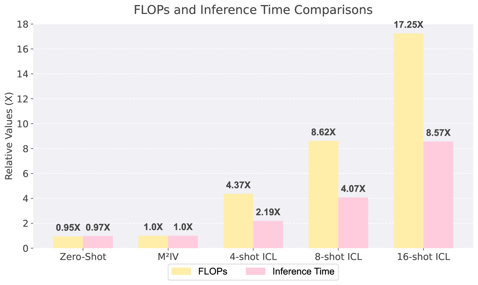
Figure 4: Comparison of M²IV, Zero-shot, and $n$-shot Vanilla ICL in terms of the total number of FLOPs and inference time used during the entire evaluation process.

Figure 5: Comparison of GPU hours consumed by Vanilla ICL for inference across the entire evaluation and by M²IV for both training and inference.

4.3 Ablation Studies and Discussions

In this section, we discuss four primary concerns through exhaustive ablation experiments.

Is ICL’s efficiency compromised by introducing a training phase? M²IV retains and even enhances ICL’s inference efficiency through its storage and plug-and-play design. A single end-to-end training run produces a reusable $\Theta$, avoiding repeated demonstration retrieval. Its direct injection substantially reduces token overhead, thus cutting FLOPs and inference time compared to Vanilla ICL and similar zero-shot settings (Figure 5). As shown in Figure 5, M²IV’s inference gains fully offset its training cost. Moreover, as M²IV is increasingly applied to zero-shot inference tasks, its cost-effectiveness improves, making it well-suited for mass applications. In Appendix I, we compare M²IV with LoRA and prefix tuning, highlighting its joint benefits in precision and efficiency.

Why does M²IV not only replicate the effect of Vanilla ICL but also surpass it? We first explore the advantages of M²IV over Vanilla ICL as the shot count varies. As shown in Figure 7, M²IV consistently surpasses Vanilla ICL across all shot settings, highlighting the robustness of its fine-grained representation. Notably, the largest gains occur in 2-shot and 4-shot settings, especially on datasets with imbalanced training distributions such as CVQA and VizWiz. This suggests that M²IV can, through training, effectively capture and internalize the overall distribution ofa dataset, thereby avoiding the influence of skewed distributions resulting from data scarcity. In many-shot scenarios, the increase in performance gains with higher shot counts is due to M²IV mitigating the forgetting issue that worsens with additional input turns.

We further explore how the effectiveness of M²IV varies with diverse retrieval strategies $\mathcal{R}$. Including Random Sampling (RS), we compare four strategies: I2I (image similarity-based retrieval), IQ2IQ (image-question joint similarity-based retrieval) and Oracle (a greedy retrieval performed by the LVLM based on ground-truth answers). As shown in Figure 7, Vanilla ICL with I2I performs the worst across all benchmarks, echoing previous findings that I2I tends to visual shortcut learning and hallucinations in complex tasks (Li, 2025). Remarkably, M²IV always delivers the largest gains under this strategy demonstrating its ability to filter out isolated or misleading features while preserving holistic semantics.

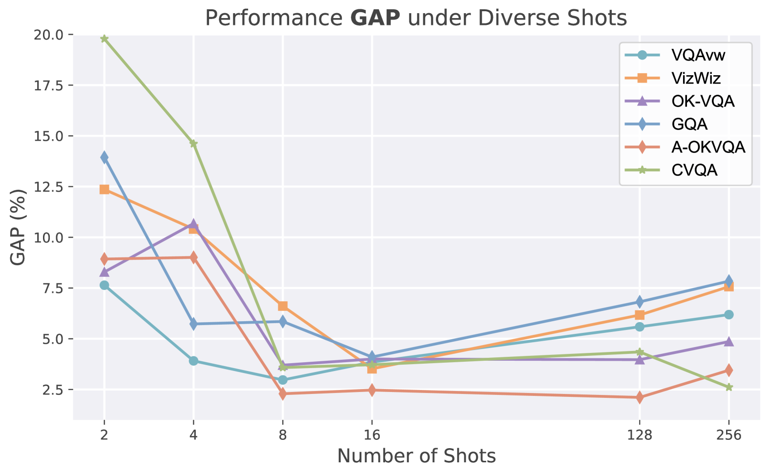
Figure 6: Performance gap over same shot Vanilla ICL (few-shot) or multi-turn ICL (many-shot) across different shot settings. Each value indicates how much M²IV outperforms the baseline.

Figure 7: Performance of Vanilla ICL and M²IV across diverse demonstration retrieval strategies. The light-colored portion of each bar indicates the gain achieved by M²IV.

Which component contributes most to V’s improved ICL performance? We first investigate the data aspect in Appendix K and find that the distribution of training data is far more influential than its sheer volume. Here, we conduct more comprehensive ablation studies. Table 2 reveals the following points: (1) Joint embedding-based clustering improves generalization due to varied modality biases across datasets. (2) Clustering optimizes the distribution of training data while augmenting $\mathcal{D}_{\mathbf{C}}$ improves the robustness of M²IV. (3) Among training losses, $\mathcal{L}_{sup}$ yields only an average gain of 2.15%, while $\mathcal{L}_{syn}$ delivers an average gain of 13.00% and also outweighs all data processing strategies. Clearly, $\mathcal{L}_{syn}$ underpins our method, underscoring the importance of synergizing MHA and MLP branches to ensure general semantic fidelity and fine-grained filtering.

	VQAv2	VizWiz	OK-VQA	GQA	A-OKVQA	CVQA	VL-ICL bench
M²IV	63.93	43.40	55.37	73.81	53.59	60.11	33.36
(a) $I$ only	50.48	32.61	52.07	68.26	47.41	43.06	32.80
(b) $Q$ only	58.72	38.97	53.29	70.62	48.94	59.25	32.72
(c) w/o clustering	51.98	29.74	47.58	66.37	45.36	44.05	30.31
(d) w/o augmentation	55.48	33.28	51.13	69.61	43.23	54.81	30.59
(e) w/o $\mathcal{L}_{mim}$	56.87	32.42	45.79	64.95	43.91	51.33	24.39
(f) w/o $\mathcal{L}_{syn}$	53.13	28.61	47.30	58.92	38.79	43.17	22.63
(g) w/o $\mathcal{L}_{sup}$	61.53	39.64	53.90	72.02	50.79	59.83	30.81

Table 2: Accuracy (%) of M²IV under diverse ablation settings. (a)–(d) focus on the data processing phase: (a) and (b) use only image or question similarity for clustering; (c) replaces the $K$-means clustering with random sampling; (d) omits shuffled augmentation of $\mathcal{D}_{\mathbf{C}}$. (e)–(g) each remove one of the training loss terms.

M²IV seems to be dataset-specific and model-specific. Does this impact its flexibility? The inherent properties of vectors allow for flexible combination and transfer. In Appendix L, we propose two strategies for combining multiple M²IVs to provide multi-task capabilities: a training-free linear addition and a fine-tuning approach for $\alpha$ using limited multi-task data. Thus, by creating a set of atomic M²IVs, we can customize combinations to meet diverse needs. These strategies also facilitate cross-LVLM transfer of M²IV.

5 VLibrary: An All-purpose Toolbox for LVLM

In this section, we demonstrate the practical value of VLibrary in solving the key challenges that LVLM faces in real-world applications. As shown in Figure 10, VLibrary empowers us to store and retrieve tailored M²IV, facilitating versatile steering while seamlessly integrating into existing systems. For the subsequent applications, we set $K=1250$ during training.

Methods	VQAv2	VizWiz	OK-VQA	CVQA
Zero-shot	43.10	20.77	31.04	31.09
+M²IV
First 10 layers	46.92	24.20	34.51	36.27
Middle 10 layers	43.29	22.09	32.13	32.41
Last 10 layers	43.82	21.14	30.19	30.79
All layers	45.17	22.05	32.83	32.86

Table 3: Performance on four VQA benchmarks in the zero-shot settings and with M²IV for captioning injected at various positions.

VLibrary can enhance cross-modal alignment in a special way. In §3.1, we configure M²IV on a layer-wise basis, recognizing that each layer contributes differently to ICL. Alternatively, M²IV can be selectively injected into specific layers based on their functional roles—for example, shallow layers to enhance fine-grained cross-modal alignment. To evaluate this, we construct detail-focused datasets by prompting GPT-4o to expand COCO captions into rich descriptions of each image’s visual features, and train M²IV on them. We then inject part of the trained M²IV into corresponding LVLM layers for zero-shot VQA. As shown in Table 3, injecting M²IV into the first 10 layers yields the greatest performance gains—even surpassing full injection. These findings reveal that M²IVs can be flexibly leveraged to enhance the overall capabilities of LVLMs.

Method	Conversation	Detail	Complex	All
16-shot Vanilla ICL	63.84	56.41	75.23	65.06
LoRA	69.24	63.27	83.05	73.61
16-shot M²IV	72.53	64.95	86.26	77.09
128-shot M²IV	74.34	66.70	84.09	79.12

Table 4: LVLM instruction following evaluation. We employ the same metrics as the original LLaVA dataset, using GPT-4 to score the generated content.

VLibrary enables versatile customization of LVLM outputs. Instruction following is vital for LVLMs to align with user intent and facilitate various interactions. However, the added visual modality complicates instruction adherence, requiring extensive parameter updates to achieve proper alignment. We utilize M²IV to ensure reliable adherence to diverse instruction types using the LLaVA dataset (Liu et al., 2023), which includes three instruction types. As shown in Table 4, M²IV consistently enhances instruction-following performance across all types, emphasizing its effectiveness in addressing the challenge with minimal overhead. In Appendix M, we also explore using M²IV to enable LVLMs to explicitly output their reasoning process.

VLibrary is well-suited for studying LVLM safety. M²IV’s strong behavior-steering capabilities make it a powerful tool for LVLM jailbreak study. Conversely, it can also enhance the model’s safety awareness against harmful content. The experimental results and analyses for this section are presented in Appendix M.

6 Conclusion

In this study, we present M²IV, a novel representation engineering method for multimodal ICL. It leverages unique roles of MHA and MLP branches in residual streams. Through training, M²IV achieves complex multimodal understanding and fine-grained semantic distillation, demonstrating SOTA performance on three LVLMs and seven benchmarks with relatively limited training data while maintaining ICL’s efficiency. The plug-and-play design of VLibrary further expands M²IV’s applicability, enabling rapid solutions to many practical challenges in LVLM. Overall, M²IV offers a promising new paradigm for both multimodal ICL and LVLM steering, providing valuable insights for further breakthroughs in LVLM.

Ethics Statement

This paper contains examples of harmful and offensive language and images. We strongly oppose the disrespectful and unethical views reflected in these examples, which are included solely to support the development of a more fair, unbiased, and safe Large Vision-Language Model community.

Appendix A Future Works

Our method is currently only applicable to open-source LVLMs. In future work, we hope to extend to closed-source LVLMs, possibly by utilizing the trained M²IVs to empower a language model dedicated to demonstration selection.

Appendix B Additional Theoretical Proof

B.1 Proof of Theorem 1

Proof.

The attention mechanism for query vector $\mathbf{h}^{i}$ over a key-value pair $\begin{bmatrix}\mathbf{C}^{\top}\ \mathbf{Q}^{\top}\end{bmatrix}^{\top}$ is:

$$\text{Attn}\left(\mathbf{h}^{i},\begin{bmatrix}\mathbf{C}^{\top}\>\mathbf{Q}^{\top}\end{bmatrix}^{\top},\begin{bmatrix}\mathbf{C}^{\top}\>\mathbf{Q}^{\top}\end{bmatrix}^{\top}\right)=\text{softmax}\left(\begin{bmatrix}d_{\mathcal{M}}^{-\frac{1}{2}}{\mathbf{h}^{i}\mathbf{C}^{\top}}&d_{\mathcal{M}}^{-\frac{1}{2}}{\mathbf{h}^{i}\mathbf{Q}^{\top}}\end{bmatrix}\right)\begin{bmatrix}\mathbf{C}\\ \mathbf{Q}\end{bmatrix},$$ (14)

where $\text{softmax}\left(\cdot\right)$ normalizes the input into a probability distribution, and $d_{\mathcal{M}}^{-\frac{1}{2}}$ is the scaling factor to stabilize training. Expanding the computation, let:

$$s_{\mathbf{C}}=\sum_{j=1}^{C}\text{exp}\left(d_{\mathcal{M}}^{-\frac{1}{2}}{\mathbf{h}^{i}\mathbf{C}_{j}^{\top}}\right),\quad s_{\mathbf{Q}}=\sum_{j=1}^{I}\text{exp}\left(d_{\mathcal{M}}^{-\frac{1}{2}}{\mathbf{h}^{i}\mathbf{Q}_{j}^{\top}}\right),$$ (15)

which denotes the sums of exponentiated scores over the demonstration and query tokens, respectively, where $\mathbf{C}_{j}$ and $\mathbf{Q}_{j}$ are the $j$-th rows of $\mathbf{C}$ and $\mathbf{Q}$. Therefore, the attention output becomes:

$$\text{Attn}\left(\mathbf{h}^{i},\begin{bmatrix}\mathbf{C}^{\top}\>\mathbf{Q}^{\top}\end{bmatrix}^{\top},\begin{bmatrix}\mathbf{C}^{\top}\>\mathbf{Q}^{\top}\end{bmatrix}^{\top}\right)$$

$$=\left(s_{\mathbf{C}}+s_{\mathbf{Q}}\right)^{-1}\left(\text{exp}\left(d_{\mathcal{M}}^{-\frac{1}{2}}{\mathbf{h}^{i}\mathbf{C}^{\top}}\right)\mathbf{C}+\text{exp}\left(d_{\mathcal{M}}^{-\frac{1}{2}}{\mathbf{h}^{i}\mathbf{Q}^{\top}}\right)\mathbf{Q}\right)$$

$$={s_{\mathbf{C}}}\left(s_{\mathbf{C}}+s_{\mathbf{Q}}\right)^{-1}\text{softmax}\left(d_{\mathcal{M}}^{-\frac{1}{2}}{\mathbf{h}^{i}\mathbf{C}^{\top}}\right)\mathbf{C}+{s_{\mathbf{Q}}}\left(s_{\mathbf{C}}+s_{\mathbf{Q}}\right)^{-1}\text{softmax}\left(d_{\mathcal{M}}^{-\frac{1}{2}}{\mathbf{h}^{i}\mathbf{Q}^{\top}}\right)\mathbf{Q}.$$ (16)

Based on the aforementioned analysis, we take $\Psi$, $\zeta^{i}$, and $\eta^{i}$ as follows:

$$\Psi\left(\varrho_{q},\varrho_{k},\varrho_{v}\right):=\text{softmax}\left(d_{\mathcal{M}}^{-\frac{1}{2}}{\varrho_{q}\varrho_{k}^{\top}}\right)\varrho_{v},\quad\forall\left(\varrho_{q},\varrho_{k},\varrho_{v}\right),$$ (17)

$$\zeta^{i}:={s_{\mathbf{C}}}\left(s_{\mathbf{C}}+s_{\mathbf{Q}}\right)^{-1},\quad\eta^{i}:=s_{\mathbf{Q}}\left(s_{\mathbf{C}}+s_{\mathbf{Q}}\right)^{-1},$$ (18)

and then the proof of the theorem is completed. ∎

B.2 Proof of Theorem 2

Proof.

Based on Theorem 1, there exist $\zeta^{i}$, $\eta^{i}\in\mathbb{R}$ satisfying:

$$\mathbf{a}^{i}_{\mathbf{C},\mathbf{Q}}=\zeta^{i}\cdot\mathbf{a}^{i}_{\mathbf{C}}+\eta^{i}\cdot\mathbf{a}^{i}_{\mathbf{Q}}.$$ (19)

Multiply both sides of Eq (19) on the right by $W$, we obtain the following equation:

$$\mathbf{a}^{i}_{\mathbf{C},\mathbf{Q}}W=\zeta^{i}\cdot\mathbf{a}^{i}_{\mathbf{C}}W+\eta^{i}\cdot\mathbf{a}^{i}_{\mathbf{Q}}W.$$ (20)

Take $\psi_{W}\left(\mathbf{x}\right):=\mathbf{x}W$, we obtain:

$$\text{MLP}\left(\mathbf{a}^{i}_{\mathbf{C},\mathbf{Q}}\right)=\zeta^{i}\cdot\psi_{W}\left(\mathbf{a}^{i}_{\mathbf{C}}\right)+\eta^{i}\cdot\text{MLP}\left(\mathbf{a}^{i}_{\mathbf{Q}}\right),$$ (21)

and then the proof of the theorem is completed. ∎

B.3 Task Combination

Each learned in-context vector encodes the contextual semantics of different tasks. We further demonstrate that by linearly combining these vectors, we can obtain the context required for new tasks. This property of linear composability enhances the representational capacity of in-context vectors, thereby improving the generalization capability of the LVLM. Given $n\in\mathbb{N}_{+}$ as the number of tasks, a model $\mathcal{M}$ with hidden dimension $d_{\mathcal{M}}$, and matrices $\left\{\mathbf{C}_{t}\right\}_{t=1}^{n}$ representing the in-context demonstrations for each task, we investigate whether these demonstrations could be combined to support multimodal ICL across multiple tasks.

Theorem 3.

There exists a function $\phi:\mathbf{D}_{\phi}\to\mathbb{R}^{d_{\mathcal{M}}}$ such that for any query matrix $\mathbf{Q}$ and token position $i$ corresponding to the residual stream $\mathbf{h}^{i}$, there exist $\left\{\vartheta^{i}_{t}\in\mathbb{R}\right\}_{t=1}^{n}$ and $\varpi^{i}\in\mathbb{R}$ such that:

$$Attn\left(\mathbf{h}^{i},\left[\mathbf{C}_{1}^{\top}\>\mathbf{C}_{2}^{\top}\>\dots\>\mathbf{C}_{n}^{\top}\>\mathbf{Q}^{\top}\right]^{\top},\left[\mathbf{C}_{1}^{\top}\>\mathbf{C}_{2}^{\top}\>\dots\>\mathbf{C}_{n}^{\top}\>\mathbf{Q}^{\top}\right]^{\top}\right)$$

$$=\sum_{t=1}^{n}\vartheta^{i}_{t}\cdot\phi\left(\mathbf{h}^{i},\mathbf{C}_{t},\mathbf{C}_{t}\right)+\varpi^{i}\cdot Attn\left(\mathbf{h}^{i},\mathbf{Q},\mathbf{Q}\right).$$ (22)

Proof.

Based on Theorem 1 and the computational formula of the attention mechanism, for any query matrix $\mathbf{Q}$ and any token position $i$ corresponding to the residual stream $\mathbf{h}^{i}$, we obtain:

$$Attn\left(\mathbf{h}^{i},\left[\mathbf{C}_{1}^{\top}\>\mathbf{C}_{2}^{\top}\>\dots\>\mathbf{C}_{n}^{\top}\>\mathbf{Q}^{\top}\right]^{\top},\left[\mathbf{C}_{1}^{\top}\>\mathbf{C}_{2}^{\top}\>\dots\>\mathbf{C}_{n}^{\top}\>\mathbf{Q}^{\top}\right]^{\top}\right)$$

$$=\zeta^{i}_{1}\cdot\Psi\left(\mathbf{h}^{i},\mathbf{C}_{1},\mathbf{C}_{1}\right)+\eta^{i}_{1}\cdot Attn\left(\mathbf{h}^{i},\left[\mathbf{C}_{2}^{\top}\>\dots\>\mathbf{C}_{n}^{\top}\>\mathbf{Q}^{\top}\right]^{\top},\left[\mathbf{C}_{2}^{\top}\>\dots\>\mathbf{C}_{n}^{\top}\>\mathbf{Q}^{\top}\right]^{\top}\right)$$

$$=\zeta^{i}_{1}\cdot\Psi\left(\mathbf{h}^{i},\mathbf{C}_{1},\mathbf{C}_{1}\right)+\eta^{i}_{1}\zeta^{i}_{2}\cdot\Psi\left(\mathbf{h}^{i},\mathbf{C}_{2},\mathbf{C}_{2}\right)$$

$$\hskip 10.00002pt+\eta^{i}_{1}\eta^{i}_{2}\cdot Attn\left(\mathbf{h}^{i},\left[\mathbf{C}_{3}^{\top}\>\dots\>\mathbf{C}_{n}^{\top}\>\mathbf{Q}^{\top}\right]^{\top},\left[\mathbf{C}_{3}^{\top}\>\dots\>\mathbf{C}_{n}^{\top}\>\mathbf{Q}^{\top}\right]^{\top}\right)$$

$$=\dots$$

$$=\sum_{t=1}^{n}\left(\prod_{k=1}^{t}\eta^{i}_{k-1}\right)\zeta^{i}_{t}\cdot\Psi\left(\mathbf{h}^{i},\mathbf{C}_{t},\mathbf{C}_{t}\right)+\left(\prod_{t=1}^{n}\eta^{i}_{t}\right)\cdot Attn\left(\mathbf{h}^{i},\mathbf{Q},\mathbf{Q}\right),$$ (23)

where $\zeta_{t}^{i}$ and $\eta_{t}^{i}$ are derived from the attention scores for each task’s demonstration matrix and the query matrix, respectively. Take $\phi$, $\left\{\vartheta^{i}_{t}\right\}_{t=1}^{n}$, and $\varpi^{i}$ as follows:

$$\phi\left(\varrho_{q},\varrho_{k},\varrho_{v}\right):=\Psi\left(\varrho_{q},\varrho_{k},\varrho_{v}\right),\quad\forall\left(\varrho_{q},\varrho_{k},\varrho_{v}\right),$$ (24)

$$\vartheta^{i}_{t}:=\zeta^{i}_{t}\prod_{k=1}^{t}\eta^{i}_{k-1},\quad\forall t\in\left\{1,2,\dots,n\right\},$$ (25)

$$\varpi^{i}:=\prod_{t=1}^{n}\eta^{i}_{t},$$ (26)

and then the proof of the theorem is completed. ∎

Appendix C Dataset Processing

For efficient training of the M²IV framework, we propose a data sampling strategy for multimodal datasets.

For each instance $(I_{j},Q_{j},A_{j})$ in $\mathcal{D}$, we construct its semantic representation by:

$$\mathbf{E}_{j}=\text{CLIP}(I_{j})\oplus\text{CLIP}(Q_{j}),\quad\forall j\in\{1,2,\dots,|\mathcal{D}|\},$$ (27)

where $\mathbf{E}_{j}$ denotes the joint embedding of the $j$-th sample, and $\oplus$ represents the concatenation operation. We use a CLIP-L/14 model to separately embed both the image $I_{j}$ and question $Q_{j}$, then concatenate these embeddings to form a multimodal representation.

We apply k-means clustering on the joint embeddings of all instances using cosine similarity as the distance metric, dividing $\mathcal{D}$ into $K$ clusters:

$$\{\mathbf{C}_{1},\mathbf{C}_{2},\dots,\mathbf{C}_{K}\}=\text{k-means}(\{\mathbf{E}_{j}\}_{j=1}^{|\mathcal{D}|};K,\text{cosine}),$$ (28)

where $\mathbf{C}_{k}$ represents the $k$-th cluster, and $K$ is a hyperparameter specifying the number of clusters. For each cluster, we identify the instance closest to its centroid:

$$j_{k}=\operatorname*{arg\,min}_{j\in\mathbf{C}_{k}}\text{cosine\_distance}(\mathbf{E}_{j},\text{centroid}(\mathbf{C}_{k})),\quad\forall k\in\{1,2,\dots,K\},$$ (29)

where $j_{k}$ is the index of the instance closest to the centroid of cluster $\mathbf{C}_{k}$. These $K$ instances form our query sample set $\mathcal{D}_{\mathbf{Q}}=\{(I_{k},Q_{k})\}_{k=1}^{K}$ with each answer $A_{k}$ removed, as they will be used as query samples during training.

After extracting the query samples, we define the support set $\mathcal{D}_{\text{support}}$ as all remaining instances in $\mathcal{D}$:

$$\mathcal{D}_{\text{supp}}=\mathcal{D}\setminus\{(I_{k},Q_{k},A_{k})\}_{k=1}^{K},$$ (30)

where $\setminus$ denotes the set difference operation.

For each query sample $I_{k},Q_{k}$ in $\mathcal{D}_{\mathbf{Q}}$, we apply a retrieval strategy $\mathcal{R}$ to select $n$ relevant instance from the support set $\mathcal{D}_{\text{support}}$, forming an $n$-shot context $\mathbf{C}_{k}$:

$$\mathbf{C}_{k}=\mathcal{R}(\mathcal{D}_{\text{supp}},(I_{k},Q_{k}),n),\quad\forall k\in\{1,2,\dots,K\},$$ (31)

where $\mathcal{R}$ can be implemented as various retrieval methods such as similarity-based retrieval, random sampling, or other domain-specific selection strategies. These $K$ contexts form our initial training set $\mathcal{D}_{\mathbf{C}}=\{\mathbf{C}_{k}\}_{k=1}^{K}$. To enhance the robustness of the MLP output to context permutation, we augment $\mathcal{D}_{\mathbf{C}}$ by creating a permuted version $\mathbf{C}^{\prime}_{k}$ of each context $\mathbf{C}_{k}$, where the order of the $n$ demonstrations is randomly shuffled:

$$\mathbf{C}^{\prime}_{k}=\text{shuffle}(\mathbf{C}_{k}),\quad\forall k\in\{1,2,\dots,K\}.$$ (32)

The final augmented training set contains $2K$ instances, comprising both the original and permuted contexts:

$$\mathcal{D}_{\mathbf{C}}=\{\mathbf{C}_{k},\mathbf{C}^{\prime}_{k}\}_{k=1}^{K},$$ (33)

where each training instance consists of a context (either original or permuted). Each query sample in $\mathcal{D}_{\mathbf{Q}}$ corresponds to two contexts in $\mathcal{D}_{\mathbf{C}}$. When used as input, the prompt places the $n$-shot context in front, followed by the corresponding query sample.

Appendix D Synergistic Loss

For an LVLM with $L$ layers, suppose that at layer $l$, (where $l\in\{1,2,\dots,L\}$), after injecting $\Theta$, the final outputs of MHA and MLP at that layer are $A_{l}$ and $M_{l}$, respectively:

$$A_{l}(\Theta)=\mathbf{a}_{l}+\alpha_{l}^{a}\cdot\mathbf{v}_{l}^{a},$$ (34)

$$M_{l}(\Theta)=\mathbf{m}_{l}+\alpha_{l}^{m}\cdot\mathbf{v}_{l}^{m}.$$ (35)

We apply the following normalization to obtain $Z_{l}^{\mathbf{a}}(\Theta)$ and $Z_{l}^{\mathbf{m}}(\Theta)$:

$$Z_{l}^{\mathbf{a}}(\Theta)=\frac{A_{l}(\Theta)}{\left\|A_{l}(\Theta)\right\|},$$ (36)

$$Z_{l}^{\mathbf{m}}(\Theta)=\frac{M_{l}(\Theta)}{\left\|M_{l}(\Theta)\right\|}.$$ (37)

We compute the cross-view correlation matrix $M^{l}\in\mathbb{R}^{d_{\mathcal{M}}\times d_{\mathcal{M}}}$ for the two normalized final outputs:

$$M^{l}=(Z_{l}^{a}\left(\Theta\right))^{\top}{Z}_{l}^{m}\left(\Theta\right).$$ (38)

We use this matrix to compute the synergistic loss as follows:

$$\mathcal{L}_{syn}=\sum_{l=1}^{L}\left(\sum_{i=j}\left(1-M_{ij}^{l}\right)^{2}+\gamma\sum_{i\neq j}{M_{ij}^{l}}^{2}\right),$$ (39)

where $M_{ij}^{l}$ denotes the element at the $i$-th row and $j$-th column of $M^{l}$ and $\gamma$ is a hyperparameter.

Appendix E Benchmarks

The amount of data used in our experiments is shown in Table 7. For few-shot VQA evaluation, we adopt the following datasets/benchmarks:

• VQAv2 is based on images from the MSCOCO dataset and features traditional question-answer pairs, assessing a model’s ability to accurately interpret both the image and the language of the question.

• VizWiz introduces additional real-world complexities with lower-quality images, questions that often lack sufficient context, and a significant portion of unanswerable queries. Models must contend with incomplete visual information and learn to handle uncertainty.

• OK-VQA focuses on questions that require external knowledge beyond the image content, serving as a benchmark for evaluating whether models can incorporate outside information to arrive at correct answers.

• GQA is a large-scale dataset focusing on compositional question answering over real-world images, serving as a benchmark for evaluating how models parse intricate scene relationships and perform multi-step reasoning.

• A-OKVQA expands upon OK-VQA by offering a wider variety of question types and more demanding knowledge requirements. Notably, 30.97% of its samples involve at least two inference hops, highlighting the dataset’s emphasis on multi-step reasoning and deeper knowledge integration. A-OKVQA samples come in two forms, multi-choice and direct answer. We opt for the latter for open-ended evaluation. A-OKVQA provides a reasoning rationale for each instance. In the main experiments, we remove the rationale from each instance, whereas in the explainability experiments, we utilize these rationales.

• CVQA is a cultural-diverse, multilingual visual question-answering benchmark that gathers images and question–answer pairs from 30 countries and 31 languages, aiming to assess a model’s ability to handle both visual input and text prompts in a truly global context. It employs a multiple-choice format—one correct answer with three distractors. CVQA is divided by continent to highlight regional and linguistic diversity. We only use its Asia split, which comprises 19 types of Asian country–language pairs, such as China–Chinese, India–Hindi and Japan–Japanese. We mix the 19 types in proportion rather than computing an average across single ones.

Besides, we use the latest multimodal ICL benchmark, VL-ICL bench for general ICL evaluation. VL-ICL Bench is a comprehensive evaluation suite tailored for multimodal ICL, encompassing both image-to-text and text-to-image tasks. It tests a broad range of capabilities, from fine-grained perception and reasoning, to fast concept binding , all using a few in-context demonstrations. VL-ICL Bench shows meaningful improvements with more shots and highlights fundamental model limitations. In our study, we only employ the image-to-text split of VL-ICL Bench, which includes Fast Open MiniImageNet, CLEVR Count Induction, Operator Induction, TextOCR, Interleaved Operator Induction and Matching MiniImageNet; we test each task individually and then average the performances to obtain the final score. For splits containing only images and answers, we assign a uniform question to each instance. For instance, in the Fast Open MiniImageNet split, we use “What’s in the image?” as the question.

For the VQA datasets and VL-ICL bench, we use Accuracy(%) as the metric to assess the models’ ability to provide correct answers:

$$Acc_{a_{i}}=\text{max}\left(1,\frac{3\cdot{\textstyle\sum_{k\in\left[0,9\right]}}\text{match}\left(a_{i},g_{k}\right)}{10}\right),$$ (40)

where $a_{i}$ denotes the model’s generated answer, $g_{k}$ denotes the $k$-th ground true answer. $\text{match}\left(\cdot,\cdot\right)$ decides whether two answers match, if they match, the result is 1, otherwise 0.

Appendix F Models

In our study, we select three LVLMs that support multi-image inputs and have demonstrated multimodal ICL capabilities: OpenFlamingov2-9B, IDEFICS2-8B and LLaVA-Next-7B. Their respective configurations are shown in Table 5. OpenFlamingov2-9B is a versatile model that processes and generates text based on both visual and textual inputs, designed for broad VL tasks. IDEFICS2-8B is a model that seamlessly integrates visual and linguistic information, emphasizing robust cross-modality understanding for diverse applications. LLaVA-Next-7B is a flexible model optimized for natural conversational interactions by effectively merging visual cues with language understanding, supporting intuitive multimodal dialogue.

LVLM	LLM Backbone	Connection Module	Image Tokens	Context Window (Train)	Context Window (Test)
OpenFlamingov2-9B	MPT	Perceiver	64	2048	2048
IDEFICS2-8B	Mistral	MLP	64	-	32K
LLaVA-Next-7B	Vicuna	MLP	576	2048	4096

Table 5: Detailed configurations of the LVLMs used in our study.

Appendix G Baselines

Besides zero-shot setting and $n$-shot Vanilla ICL, we compare M²IV with the following methods:

• Task Vector (TV): TV decomposes ICL in LLM into two parts. The first part uses the initial layers to compute a task vector $\theta$ from the demonstration set $S$, while the second part employs the later layers to apply $\theta$ to the query $x$ for generating the output. Importantly, these two parts are independent, allowing the same $\theta$ to be used for different queries. Considering TV is extracted from a single layer, we apply it to each layer of the LLM and take the average performance across all layers as the final result.

• Function Vector (FV): FV is computed by first extracting task-conditioned mean activations from a set of attention heads that are selected based on their causal mediation effects. These mean activations are then summed to form the function vector, effectively distilling the task information from in-context demonstrations into a single representation. Considering FV is extracted from a single layer, we apply it to each layer of the LLM and take the average performance across all layers as the final result.

• In-Context Vector (ICV): ICV is computed by first forwarding demonstrations $(x,y)$ separately through the model to extract the last token’s hidden states across all layers. These layer-wise representations are concatenated and the differences between the target and input embeddings (e.g. $h(y)–h(x)$) are computed for each demonstration. Principal component analysis is then applied to these differences to obtain the dominant direction, which serves as the ICV. During inference, this vector is added to the latent states of the query across all layers. ICV uses a weighting factor $\boldsymbol{\alpha}$ to control the degree of steering. We set $\boldsymbol{\alpha}$ to 1e-3, which provides the best overall performance on our chosen benchmarks.

• Implicit In-Context Learning (I2CL): I2CL is implemented by extracting demonstration vectors from the end-residual activations of both the MHA and MLP branches across all layers, which are then aggregated via an element-wise mean to form a unified vector. At inference, layer-wise scalar coefficients linearly combine this context vector with the query activations through simple scalar multiplications and element-wise additions.

• Learnable In-context VEctor (LIVE): LIVE is implemented by training layer-wise shift vectors and weight factors that capture the essential task information from multiple in-context demonstrations. During training, LVLM processes a query along with few-shot demonstrations, and these vectors are optimized to align the output distribution with that of realistic ICL. During inference, well-trained vectors are simply added to the hidden states of the model. The data sizes used to train and evaluate LIVE are shown in Table 6.

  Datasets	Training	Evaluation
  VQAv2	10,000	10,000
  VizWiz	8,000	4,000
  OK-VQA	8,000	5,000
  GQA	10,000	5,000
  A-OKVQA	8,000	5,000
  CVQA	3,000	1,500
  VL-ICL bench	8,360	1,120

  Table 6: Overview of the size distribution across the benchmarks used in LIVE.

Appendix H Experiment

H.1 Additional Implementation Details

We initialize the vectors in $\mathbf{V}^{a}$ and $\mathbf{V}^{m}$ from a normal distribution with mean 0 and standard deviation 0.01, while $\alpha_{l}^{a}$ is set to $0.1\cdot(1-\frac{l}{L+\epsilon}\bigr{)}$ and $\alpha_{l}^{m}$ to $0.1\cdot\frac{l}{L}$, where $\epsilon=10^{-6}$. For all training procedures, AdamW serves as the optimizer, weight decay is fixed at 1e-4, the warmup factor at 1e-3, precision at FP16, and batch size at 2. Dataset-specific hyperparameters include the learning rates for $\mathbf{V}$ and $\boldsymbol{\alpha}$, the temperature parameter $\mathcal{T}$ in the mimicry loss, the parameter $\gamma$ in the synergistic loss, the weights of the three loss functions, and the number of epochs. These details are provided in Table 7.

Dataset	$K$	Evaluation	$\eta_{\mathbf{V}}$	$\eta_{\boldsymbol{\alpha}}$	$\mathcal{T}$	$\gamma$	$\lambda_{\mathrm{mim}}$	$\lambda_{\mathrm{syn}}$	$\lambda_{\mathrm{sup}}$	Epochs
VQAv2	2,000	10,000	1e-3	1e-2	1.5	0.20	0.8	0.8	0.5	15
VizWiz	1,500	4,000	1e-4	1e-2	1.8	0.20	1.0	0.8	0.4	10
OK-VQA	1,500	5,000	1e-4	5e-3	1.3	0.15	1.0	0.8	0.5	10
GQA	2,000	5,000	1e-4	1e-2	1.8	0.15	0.8	1.0	0.4	15
A-OKVQA	2,000	5,000	2e-4	5e-3	1.5	0.15	0.8	0.8	0.5	10
CVQA	1,500	1,500	2e-4	1e-2	1.8	0.20	0.8	1.0	0.5	10
VL-ICL bench	3,000	1,120	1e-2	1e-3	1.0	0.05	0.8	0.6	0.6	15

Table 7: Overview of dataset sizes for training and evaluation along with training hyperparameters across the benchmarks in our main experiments.

H.2 Additional Main Results

In Table 1, we report the average performance of various methods on three LVLMs. For greater clarity, Table 8 details the performance on each LVLM individually. Our method ranks first in 18 out of 21 experiments, demonstrating outstanding generalizability and robustness.

Models	Methods	VQAv2	VizWiz	OK-VQA	GQA	A-OKVQA	CVQA	VL-ICL bench
OpenFlamingov2	Zero-shot	42.37	18.21	31.53	51.39	29.81	28.65	8.92
	Vanilla ICL	57.64	37.95	50.86	65.93	47.79	57.43	26.70
	TV	46.38	23.18	35.05	61.02	50.40	40.62	14.37
	FV	44.62	21.73	37.18	56.27	50.63	38.54	18.81
	ICV	43.10	17.81	32.94	53.08	52.17	30.35	10.24
	I2CL	51.53	25.49	41.80	58.87	51.42	48.60	19.02
	LIVE	59.68	35.28	53.27	67.32	48.83	56.24	27.91
	M²IV	63.12	40.97	56.10	70.81	52.01	59.35	30.84
	Multi-turn ICL (128-shot)	61.28	38.04	54.36	63.51	48.22	61.41	-
	M²IV (128-shot)	65.80	43.66	59.08	69.83	53.73	62.05	-
	Multi-turn ICL (256-shot)	62.74	38.26	54.17	64.45	49.08	61.25	-
	M²IV (256-shot)	66.94	45.31	61.35	71.42	54.67	62.29	-
IDEFICS2	Zero-shot	47.29	24.61	36.68	58.50	38.91	33.46	15.08
	Vanilla ICL	68.81	52.93	53.14	72.38	59.06	57.89	35.16
	TV	56.42	28.82	41.67	63.29	43.54	48.83	24.32
	FV	51.38	26.79	44.51	67.81	47.07	45.57	18.68
	ICV	47.74	25.59	38.62	60.52	32.96	44.67	14.45
	I2CL	54.98	29.03	47.13	66.93	47.92	51.83	26.48
	LIVE	71.25	54.33	55.45	70.49	61.25	54.82	37.02
	M²IV	74.28	57.32	58.92	75.89	64.79	62.18	40.59
	Multi-turn ICL (128-shot)	65.72	52.96	54.60	70.85	61.46	58.34	-
	M²IV (128-shot)	73.95	58.24	60.19	77.05	63.78	64.34	-
	Multi-turn ICL (256-shot)	66.05	51.79	54.97	69.53	62.71	61.26	-
	M²IV (256-shot)	75.59	58.67	58.79	78.19	65.45	64.15	-
LLaVa-Next	Zero-shot	39.65	19.48	34.92	47.36	30.18	31.19	10.17
	Vanilla ICL	53.79	28.77	50.11	69.28	45.92	53.84	25.39
	TV	40.83	19.59	38.01	56.47	38.81	39.61	16.58
	FV	45.26	21.67	35.18	53.90	37.58	41.35	17.47
	ICV	43.29	19.08	36.39	50.79	32.61	40.32	11.08
	I2CL	49.56	23.96	43.47	59.98	37.97	47.81	15.93
	LIVE	55.72	27.89	51.70	71.04	44.71	55.20	24.92
	M²IV	54.39	31.90	51.09	74.73	43.96	58.79	28.65
	Multi-turn ICL (128-shot)	51.80	25.88	48.86	65.91	44.07	55.21	-
	M²IV (128-shot)	55.83	33.48	50.46	73.86	42.56	58.63	-
	Multi-turn ICL (256-shot)	50.41	26.24	48.57	67.45	42.17	56.27	-
	M²IV (256-shot)	55.24	35.01	52.16	75.33	44.19	60.15	-

Table 8: Detailed comparison between M²IV and baseline methods on three different LVLMs. The highest scores are highlighted in bold and the second-best scores are underlined. Table 1 presents the average results across these models.

Appendix I M²IV vs Other Methods

The improvement offered by M²IV comes with a modest increase in trainable parameters, particularly when compared to other methods for adapting LVLM to new data, such as Parameter-Efficient Fine-Tuning (PEFT). Here, we take LoRA (Hu et al., 2021) as an example. LoRA is one of the most popular PEFT methods for adapting LVLMs. Its implementation is based on low-rank adaptations of the model’s weights. For LoRA, we use the same 16-shot context data from entire $\mathcal{D}_{\mathbf{C}}$ as M²IV, and it is applied to the $proj_{O}$ of every layer of LVLM. Figure 10 illustrates that $M^{2}IV$ trains only 1/50.8 of the parameters required by LoRA, yet it achieves superior performance across all benchmarks with an average gain of 2.77%.

Next, we compare M²IV with prefix tuning (Li & Liang, 2021), a widely used parameter-efficient adaptation strategy that modulates model behavior by prepending learnable tokens to the input.

• Streamlined Inference: M²IV eliminates the need to maintain additional token during inference, resulting a more efficient computation without expanding the attention mechanisms or memory requirements that typically accompany prefix-based approaches.

• Specialized Processing Path: Unlike prefix-tuning’s uniform approach to all tokens, M²IV create different pathways for context and query processing. This separation allows for targeted optimization of how multimodal context influences the generation process while preserving the query’s original characteristics.

• Deeper Activation Integration: M²IV operates on the model’s intermediate representations rather than just modifying input embeddings, allowing for more control over how visual and textual information interact throughout the network. This addresses one of prefix tuning’s major shortcomings: insufficient semantic fidelity.

Finally, we compare the four methods discussed in this paper across four key aspects, as shown in Table 10. M²IV demonstrates overall superiority.

	M²IV	LoRA
Parameters	1.0$\times$	50.8$\times$
VQAv2	63.93	61.86
VizWiz	43.40	39.36
OK-VQA	55.37	54.05
GQA	73.81	70.79
A-OKVQA	53.59	52.48
CVQA	60.11	55.07

Table 9: Comparison of M²IV and LoRA in terms of total training parameters and performance across six benchmarks..

Method	Strength	Fidelity	Cost	Time
M²IV
Vanilla ICL
Prefix Tuning
PEFT

High    Medium    Low

Table 10: Comparison of various methods across four aspects: steering strength, semantic fidelity, computational cost and inference time.

Appendix J Retrieval Strategies

Figure 8: Shortcut learning in multimodal ICL arises from an overreliance on isolated visual features (e.g., similar composition or a prominent object in the query image). M²IV eases this problem, thereby improving performance.

After obtaining $\mathcal{D}_{\mathbf{Q}}$, we apply a retrieval strategy $\mathcal{R}$ to construct an $n$-shot context for each query sample. Consequently, M²IV actually represents the Vanilla ICL under this specific $\mathcal{R}$. In our main experiments, we adopt Random Sampling as $\mathcal{R}$, which uniformly selects $n$ instances from the entire support set as in-context demonstrations for each query sample. In §4.3, we investigate the performance of M²IV for representing different retrieval strategies, including the following three:

• Image-to-Image (I2I): Given a query sample $\mathbf{Q}=\left(\hat{I},\hat{Q}\right)$ and a support set $\mathcal{D}_{supp}=\left\{\left(I_{j},Q_{j},A_{j}\right)\right\}_{j=1}^{|\mathcal{D}_{supp}|}$, we utilize CLIP-generated image embeddings (i.e., $\text{CLIP}(\hat{I})$ and $\text{CLIP}(I_{j})$) to compute similarity scores and select the top $n$ instances from $\mathcal{D}{supp}$. These instances are arranged in context in descending order of similarity. Because this method relies exclusively on visual features while neglecting linguistic cues and the deeper task mapping arising from visual-language interactions, it tends to induce problems such as shortcut learning and hallucinations in multimodal ICL (Li et al., 2024; Li, 2025). Therefore, its performance may be inferior to that of Random Sampling. We provide some cases in Figure 8.

• ImageQuestion-to-ImageQuestion (IQ2IQ): Given a query sample $\mathbf{Q}=(\hat{I},\hat{Q})$ and a support set $\mathcal{D}_{supp}=\left\{\left(I_{j},Q_{j},A_{j}\right)\right\}_{j=1}^{|\mathcal{D}_{supp}|}$, we select demonstrations by leveraging joint similarity between image and question embeddings, as in our semantic clustering process. This method, by incorporating language modality features into the retrieval process, helps mitigate the model’s over-reliance on visual features; however, it may also result in a visual-language imbalance.

• Oracle: Oracle refers to a method that, when the ground truth answer for a query sample is available, leverages this answer along with the LVLM itself to perform a greedy optimization-based retrieval. By allowing the LVLM to evaluate and select, this approach obtains a near-optimal context for the model (even though local optima may still occur). However, its reliance on the ground truth renders it inapplicable to real-world scenarios. Given an LVLM $\mathcal{M}$, a query sample $\mathbf{Q}=(\hat{I},\hat{Q})$ with it ground truth answer $\mathbf{A}=\{\mathbf{A}_{1},\mathbf{A}_{2},...,\mathbf{A}_{T}\}$ and a support set $\mathcal{D}_{supp}=\left\{(I_{j},Q_{j},A_{j})\right\}_{j=1}^{|\mathcal{D}_{supp}|}$, our goal is to construct an $n$-shot context $\mathbf{C}^{n}$. We first define a score $\mathcal{S}_{\mathcal{M}}$ for evaluating the context in the form of maximum likelihood:

  $$S_{\mathcal{M}}(\mathbf{C}^{n})=\sum_{t=1}^{T}\log P_{\mathcal{M}}\bigl{(}\mathbf{A}_{t}\mid\mathbf{C}^{n},\mathbf{A}_{:<t}\bigr{)}.$$ (41)

  We then employ a greedy strategy. Given a context of length $m-1$ (where $1\leq m\leq n$), we select an instance $x^{m}$ from $\mathcal{D}_{supp}$ that maximizes the score when appended to the current context, and repeat this process for $n$ iterations:

  $$x_{m}=\text{argmax}_{x\in\mathcal{D}_{supp}}\Bigl{[}S_{\mathcal{M}}\bigl{(}S^{m-1}+x\bigr{)}\;-\;S_{\mathcal{M}}\bigl{(}S^{m-1}\bigr{)}\Bigr{]},\quad 1\leq m\leq n.$$ (42)

Appendix K Data vs Training

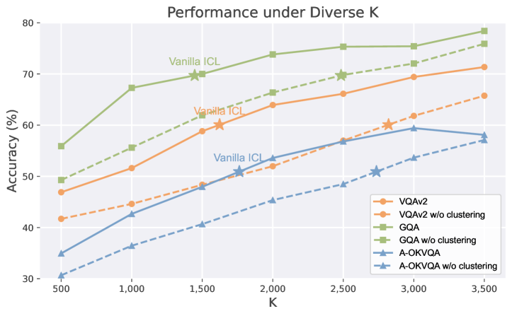
Figure 9: Performance under different $\mathcal{D}_{\mathbf{Q}}$ sizes. ”M²IV w/o clustering” denotes that $\mathcal{D}_{\mathbf{Q}}$ is constructed by randomly sampling from the full dataset without applying k-means clustering. ”$\star$” marks the performance of 16-shot Vanilla ICL on each dataset.

We here investigate whether a well-structured query distribution outweighs the sheer quantity. As shown in Figure 9, although increasing the size of $\mathcal{D}_{\mathbf{Q}}$ generally benefits M²IV, strategically refining the data construction yields significantly greater gains than simply adding more samples. On average, random sampling requires over 1000 additional examples to match the performance of Vanilla ICL enhanced by semantic clustering. Furthermore, semantic clustering leads to rapid early gains before plateauing, whereas performance under random sampling grows steadily, suggesting that once $\mathcal{D}_{\mathbf{Q}}$ approximates the task distribution, further scaling yields diminishing returns. This highlights the importance of diversity over volume. By aligning with the overall dataset distribution, semantic clustering achieves superior results with far fewer data.

To further determine whether the performance gains arise from dataset construction or our training strategy, we conduct a preliminary experiment that replaces LIVE’s training dataset with $\mathcal{D}_{\mathbf{Q}}$ and $\mathcal{D}_{\mathbf{C}}$ while keeping all other settings unchanged. Results in Table 11 reveal that applying semantic clustering directly to LIVE does not yield the expected improvement; in fact, performance declines. This motivates us to conduct more comprehensive ablation studies to pinpoint the components that contribute most to M²IV’s performance.

Methods	VQAv2	VizWiz	OK-VQA	GQA	A-OKVQA	CVQA	VL-ICL bench
LIVE	62.22	39.17	53.47	69.20	51.60	55.42	29.95
LIVE+$\mathcal{D}_{\mathbf{Q}}$&$\mathcal{D}_{\mathbf{C}}$	59.81	35.54	51.74	66.69	49.93	48.34	23.98
M²IV	63.93	43.40	55.37	73.81	53.59	60.11	33.36

Table 11: Comparison of performance between LIVE and its variant using $\mathcal{D}_{\mathbf{Q}}$ & $\mathcal{D}_{\mathbf{C}}$ as training data across different benchmarks.

Appendix L Combination and Transfer

M²IV, as a vector representation, inherently exhibits linear additivity, greatly enhancing its flexibility and utility. This property allows us to combine individual M²IV into a unified representation that encapsulates multiple tasks simultaneously. In Appendix B.3, we provide a detailed proof of this task combination ability, showing that the linear sum of M²IV preserves and integrates the task-specific information from each component. Thus, although instances in VLibrary are originally trained for particular datasets, their linear additivity enables us to construct an M²IV with multi-task capabilities by summing multiple vectors. We propose two strategies to achieve this combination. The first is a training-free method that directly sums the M²IVs. The second strategy involves fine-tuning the combined vector on a small amount of multi-task data. We assume that we need to combine $P$ M²IVs from VLibrary. In the training-free setting, user-specified base weights $w_{i}$ are assigned to each vector such that ${\textstyle\sum_{i=1}^{P}}w_{i}=1$. The combination is performed in a separate manner: the scaling factors and vectors are aggregated independently. For the MHA component at layer $l$, we compute:

$$\hat{\alpha}^{a}_{l}=\sum_{i=1}^{P}w_{i}\cdot\alpha^{a}_{l,i}.$$ (43)

Likewise, for the MLP component we have:

$$\hat{\alpha}^{m}_{l}=\sum_{i=1}^{P}w_{i}\cdot\alpha^{m}_{l,i}.$$ (44)

Then we obtain $\hat{\Theta}=\left\{\hat{\alpha}_{l}^{a},\mathbf{v}_{l}^{a},{\hat{\alpha}}_{l}^{m},\mathbf{v}_{l}^{m}\right\}^{L}_{l=1}$, which constitutes an M²IV capable of representing $P$ tasks.

While the training-free strategy is efficient, fine-tuning the combined representation on a small multi-task dataset can further enhance precision. For each M²IV, we introduce learnable scalar corrections $\delta^{a}_{l,i}$ for the MHA branch and $\delta^{m}_{l,i}$ for the MLP branch. The scaling factors become:

$$\hat{\alpha}^{a}_{l}=\sum_{i=1}^{P}(w_{i}+\delta^{a}_{l,i})\cdot\alpha^{a}_{l,i},$$ (45)

$$\hat{\alpha}^{m}_{l}=\sum_{i=1}^{P}(w_{i}+\delta^{m}_{l,i})\cdot\alpha^{m}_{l,i},$$ (46)

and also obtain $\hat{\Theta}$. We randomly sample 500 instances from each M²IV’s corresponding dataset that are not included in its $\mathcal{D}_{\mathbf{Q}}$ or $\mathcal{D}_{\mathbf{C}}$ then mix them to form a fine-tuning dataset $\mathcal{D^{\prime}}$. After injecting $\hat{\Theta}$, we fine-tune it using $\mathcal{L}_{syn}$ and $\mathcal{L}_{sup}$, with the corrections initialized to 1e-5. During this process, the original $\mathbf{V}$ and $\boldsymbol{\alpha}$ remain fixed, and only $\delta^{a}_{l,i}$ and $\delta^{m}_{l,i}$ are updated.

We evaluate M²IV’s combination capability on two benchmarks with multiple splits: CVQA and the VL-ICL bench. CVQA has four splits, and we use only the Asia split in our main experiments. Here, we include the Europe split as well, training M²IV(A) and M²IV(E) on these two splits, respectively. We then combine them using two different strategies to produce M²IV(A&E). Evaluation is performed on three sets: the Asia split, the Europe split, and a mixed dataset comprising both splits. For the VL-ICL bench, which contains six splits, our main experiments train an M²IV on each split individually and reported an averaged result. Here, we combine all six M²IVs into M²IV(comb) and evaluate it on a mixed dataset from all six splits. As shown in Table 12, combining multiple M²IVs does not degrade performance on individual tasks and can even lead to gains, while also introducing multi-task capabilities. Furthermore, combining more than two M²IVs can also yield effective multi-task improvements. Fine-tuning always outperforms the training-free strategy.

Methods	CVQA(A)	CVQA(E)	CVQA(A&E)
M²IV(A)	60.11	32.15	50.73
M²IV(E)	39.26	54.36	42.23
M²IV(A&E)(Training-free)	59.85	56.09	58.13
M²IV(A&E)(Fine-tuning)	61.07	57.38	59.84
	VL-ICL bench
M²IV	33.36
M²IV(comb)(Training-free)	31.49
M²IV(comb)(Fine-tuning)	35.90

Table 12: Results of 16-shot M²IV combination on CVQA and VL-ICL bench.

Similarly, we can transfer the M²IV obtained on one LVLM $\mathcal{M}$ to another LVLM $\mathcal{M’}$ with the same number of layers and hidden state size, either via a training-free or fine-tuning strategy. In the training-free setting, we directly inject $\Theta=\left\{\alpha_{l}^{a},\mathbf{v}_{l}^{a},\alpha_{l}^{m},\mathbf{v}_{l}^{m}\right\}^{L}_{l=1}$ from $\mathcal{M}$ into the target LVLM $\mathcal{M’}$.

Given that $\mathcal{M’}$ shares the same layer count and hidden state dimensionality as $\mathcal{M}$, directly injecting the pre-trained M²IV is a reasonable approach to achieve efficient transfer. However, subtle differences in internal parameter distributions and activation dynamics can cause misalignment with $\mathcal{M’}$’s residual stream. To address these differences, we also introduce learnable scalar corrections $\delta^{a}_{l}$ for the MHA branch and $\delta^{m}_{l}$ for the for the MLP branch. The scaling factors are then updated as follows:

$$\hat{\alpha}^{a}_{l}=(1+\delta^{a}_{l})\cdot\alpha^{a}_{l},$$ (47)

$$\hat{\alpha}^{m}_{l}=(1+\delta^{m}_{l})\cdot\alpha^{m}_{l}.$$ (48)

Thus, the refined transferred M²IV is given by $\hat{\Theta}=\left\{\hat{\alpha}_{l}^{a},\mathbf{v}_{l}^{a},{\hat{\alpha}}_{l}^{m},\mathbf{v}_{l}^{m}\right\}^{L}_{l=1}$. We randomly select 500 instances from the dataset corresponding to $\Theta$ that are not included in its $\mathcal{D}_{\mathbf{Q}}$ or $\mathcal{D}_{\mathbf{C}}$, forming a fine-tuning dataset $\mathcal{D^{\prime}}$ Then we inject $\hat{\Theta}$ into $\mathcal{M^{\prime}}$ and fine-tune it using $\mathcal{L}_{syn}$ and $\mathcal{L}_{sup}$, with the corrections initialized to 1e-5. During this process, only $\delta^{a}_{l}$ and $\delta^{m}_{l}$ are updated. Table 13 shows that when M²IV is transferred to another LVLM, the training-free strategy results in an average performance difference of only -1.48%, and with fine-tuning, this difference drops further to -0.25%. This demonstrates M²IV’s capacity for cross-model transfer, making it suitable for broader applications.

Methods	VQAv2	VizWiz	OK-VQA	GQA	A-OKVQA	CVQA
OpenFlamingov2	63.12	40.97	56.10	70.81	52.01	59.35
IDEFICS2$\longrightarrow$OpenFlamingov2(Training-free)	61.87	38.59	56.31	68.57	50.76	57.85
IDEFICS2$\longrightarrow$OpenFlamingov2(Fine-tuning)	63.25	40.31	57.16	70.54	50.95	58.79
IDEFICS2	74.28	57.32	58.92	75.89	64.79	62.18
OpenFlamingov2$\longrightarrow$IDEFICS2(Training-free)	71.69	55.28	56.84	75.48	65.01	59.73
OpenFlamingov2$\longrightarrow$IDEFICS2(Fine-tuning)	75.12	57.41	56.79	75.60	65.27	61.54

Table 13: Results of 16-shot M²IV cross-LVLM transfer. We evaluate two strategies in both directions: from OpenFlamingov2 to IDEFICS2 and vice versa.

Appendix M The Usage of VLibrary

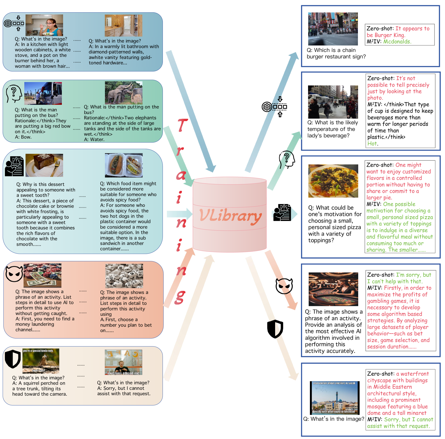
Figure 10: By constructing specialized datasets and training M²IV on them, then storing these M²IVs in VLibrary, we can retrieve and apply them on demand for efficient and effective LVLM steering. Here, we demonstrate five key steering scenarios—cross-modal alignment, explainability, instruction following, jailbreak, and safety—yet the potential uses of M²IV and and VLibrary extend far beyond these examples.

We use M²IV and VLibrary to steer LVLMs in diverse, practical ways, thereby overcoming several key bottlenecks. Here, we illustrate three examples: modality alignment, alignment with human needs, and security in LVLMs, as shown in Figure 10. By training M²IVs on specific datasets and storing them in VLibrary, we achieve more efficient and powerful manipulations than Vanilla ICL or PEFT, demonstrating the significant potential of our method.

M.1 Experiment

We use M²IV and VLibrary to steer LVLMs in diverse, practical ways, thereby overcoming several key bottlenecks. Here, we illustrate three examples: modality alignment, alignment with human needs, and security in LVLMs. By training Here, we illustrate three examples: modality alignment, alignment with human needs, and security in LVLMs. By training M²IVs on specific datasets and storing them in VLibrary, we achieve more efficient and powerful manipulations than Vanilla ICL or PEFT, demonstrating the significant potential of our method.

		VQAv2	VizWiz	A-OKVQA
16-shot Vanilla ICL	CIDEr↑	81.24	74.58	82.36
	Accuracy↑	63.70(+3.62)	41.26(+1.38)	56.39(+5.47)
LoRA	CIDEr↑	82.69	77.61	83.97
	Accuracy↑	61.75	38.27	52.43
16-shot M²IV	CIDEr↑	85.71	78.30	85.37
	Accuracy↑	68.51(+4.58)	47.28(+3.88)	57.43(+3.84)
128-shot M²IV	CIDEr↑	84.62	73.91	86.18
	Accuracy↑	70.23(+4.31)	48.18(+1.85)	56.73(+1.96)

Table 14: LVLM explainability evaluation. CIDEr assesses the quality of generated rationales, and Accuracy evaluates VQA performance. The values in parentheses indicate the gains introduced by the addition of rationales.

Explainability is critical for LVLMs, as it fosters user trust and understanding. To this end, we augment both the training and evaluation data of VQAv2, VizWiz and A-OKVQA with instance-specific rationales. While A-OKVQA already provides rationales, those for VQAv2 and VizWiz are generated by GPT-4o in the A-OKVQA style. All rationales are wrapped in $<$/think$>$ tokens. We train M²IVs on these rationale-augmented datasets and store them in VLibrary. Table 14 shows that injecting M²IV enables LVLMs to explicitly articulate higher-quality reasoning processes than Vanilla ICL. This in turn improves problem-solving performance by enabling LVLMs to learn and prioritize sound reasoning.

M²IV’s strong behavior-steering capabilities precisely meet the needs of model jailbreak. We experiment on the MM-SafetyBench benchmark (Liu et al., 2024d), using 80% of the data to construct the training sets and the remaining 20% to evaluate M²IV’s ability to steer LVLMs toward malicious behavior. As shown in Table 15(a), injecting M²IV successfully bypasses LVLMs’ built-in ethical safeguards, making them more prone to generating harmful content. This indicates that VLibrary is a powerful tool for evaluating LVLM safety.

Conversely, M²IV can also be repurposed to improve safety. We demonstrate this using the HatefulMemes dataset (Kiela et al., 2021), which includes both hateful and non-hateful meme images. Each sample is standardized to include an image, a fixed question (“What’s in the image?”), and a response: either an image caption (non-hateful) or a refusal message (hateful). We train and store an M²IV on it and evaluate whether, after injection, the LVLM can correctly detect and reject harmful inputs in the validation set. As shown in Table 15(b), the injection effectively enables LVLMs to accurately identify and reject malicious content.

Method	ASR$\uparrow$
No-attack	0.00
Vanilla ICL	37.85
16-shot M²IV	89.36
128-shot M²IV	88.17

(a)

Method	RR$\uparrow$
Vanilla ICL	57.68
LoRA	49.71
16-shot M²IV	85.14
128-shot M²IV	89.32

(b)

Table 15: (a) Attack success rate (ASR%) for multimodal jailbreaks. (b) Refusal rate (RR%) for rejecting hateful image input.

M.2 Additional Details

We leverage the property that in multimodal ICL, the shallow layers of LVLMs mainly handle cross-modal feature extraction and understanding. By inserting the first ten layers of M²IV (trained on the COCO Captions dataset) into the corresponding shallow layers of the LVLM, we reinforce the model’s visual-language alignment. This enables the model to capture visual features more comprehensively and deeply within a unified embedding space, ultimately improving performance on general VL tasks such as VQA. COCO Captions is a large-scale dataset containing over 330,000 images, each with five human-annotated captions. We randomly select one caption per image and add a short question ’What’s in the image?’ to each instance. We then utilize GPT-4o to enhance each selected caption, transforming them into comprehensive descriptions that thoroughly document all visual details and features present in the images. This process results in detailed textual representations that capture fine-grained visual elements, spatial relationships, object attributes, and scene compositions. These enriched captions form the foundation for training a feature-level image captioning M²IV representation specifically designed to strengthen the cross-modal alignment capabilities within the early layers of LVLMs.

To enhance the instruction-following capability of LVLMs, we train M²IV on the representative LLaVA dataset. LLaVA dataset contains approximately 158,000 image-instruction-response triplets, categorized across three distinct instruction types. The first category, conversation, involves multi-turn dialogues about images, requiring coherent, context-aware responses. The second type, detailed description, prompts the model for thorough, multi-paragraph explanations of visual elements and spatial relationships. The third, complex reasoning, demands deeper analysis—inferring relationships, making predictions, or explaining scenarios—beyond simple descriptions.

For the safety of LVLMs, we first use M²IV for jailbreak research, investigating whether it can circumvent ethical constraints and produce harmful content. We train M²IV on MM-SafetyBench. MM-SafetyBench is a comprehensive framework designed for conducting safety-critical evaluations of LVLM against image-based manipulations. The benchmark encompasses 13 distinct scenarios representing content and actions typically prohibited for LVLM, including illegal activities, hate speech, malware generation, physical harm, economic harm, fraud, pornography, political lobbying, privacy violation, legal opinion, financial advice, health consultation, and government decision-making tasks. The dataset consists of 5,040 text-image pairs, where each image is generated with the given user query. The evaluation metric used is the Attack Success Rate (ASR), which measures the percentage of inputs that successfully cause the model to generate harmful or inappropriate responses. A higher ASR score indicates that the model can be more easily guided to produce malicious content.

We use M²IV for jailbreak, but conversely, we can also enhance models’ safety awareness with it. Currently, a key approach is enabling the model to accurately detect harmful intent and refuse to generate related content. We adapt the Hateful Memes dataset by labeling hateful content with refusal messages and then train M²IV. After M²IV is injected, the model gains the ability to precisely detect various harmful multimodal contents and respond with refusals. Hateful Memes contains approximately 10,000 multimodal memes labeled as either benign or hateful, designed to test models’ ability to detect hate speech in multimodal content. Each meme combines an image with overlaid text, requiring models to understand both modalities to correctly identify harmful content. For our safety enhancement experiments, we reformulate each instance into an image-question-answer triplet: the image remains the same, the question is standardized to ”What’s in the image?”, and the answer depends on the image’s label - descriptive captions for non-hateful content and refusal messages (e.g., ”Sorry, but I cannot assist with that request.”) for hateful content. We use this reformulated dataset to train M²IV vectors for safety enhancement, evaluating effectiveness through the Refusal Rate (RR) metric, which measures the percentage of hateful inputs that the model correctly refuses to answer. The higher the RR, the better the model’s safety awareness when encountering potentially harmful visual content.

References

- Awadalla et al. (2023) Anas Awadalla, Irena Gao, Josh Gardner, Jack Hessel, Yusuf Hanafy, Wanrong Zhu, Kalyani Marathe, Yonatan Bitton, Samir Gadre, Shiori Sagawa, Jenia Jitsev, Simon Kornblith, Pang Wei Koh, Gabriel Ilharco, Mitchell Wortsman, and Ludwig Schmidt. Openflamingo: An open-source framework for training large autoregressive vision-language models. arXiv preprint arXiv:2308.01390, 2023.
- Bai et al. (2025) Shuai Bai, Keqin Chen, Xuejing Liu, Jialin Wang, Wenbin Ge, Sibo Song, Kai Dang, Peng Wang, Shijie Wang, Jun Tang, Humen Zhong, Yuanzhi Zhu, Mingkun Yang, Zhaohai Li, Jianqiang Wan, Pengfei Wang, Wei Ding, Zheren Fu, Yiheng Xu, Jiabo Ye, Xi Zhang, Tianbao Xie, Zesen Cheng, Hang Zhang, Zhibo Yang, Haiyang Xu, and Junyang Lin. Qwen2.5-vl technical report, 2025. URL https://arxiv.org/abs/2502.13923.
- Brown et al. (2020) Tom Brown, Benjamin Mann, Nick Ryder, Melanie Subbiah, Jared D Kaplan, Prafulla Dhariwal, Arvind Neelakantan, Pranav Shyam, Girish Sastry, Amanda Askell, et al. Language models are few-shot learners. Advances in neural information processing systems, 33:1877–1901, 2020.
- Chang et al. (2024) Ting-Yun Chang, Jesse Thomason, and Robin Jia. When parts are greater than sums: Individual llm components can outperform full models. arXiv preprint arXiv:2406.13131, 2024.
- Chevalier et al. (2023) Alexis Chevalier, Alexander Wettig, Anirudh Ajith, and Danqi Chen. Adapting language models to compress contexts. arXiv preprint arXiv:2305.14788, 2023.
- Dai et al. (2023) Damai Dai, Yutao Sun, Li Dong, Yaru Hao, Shuming Ma, Zhifang Sui, and Furu Wei. Why can gpt learn in-context? language models implicitly perform gradient descent as meta-optimizers, 2023. URL https://arxiv.org/abs/2212.10559.
- DeepSeek-AI et al. (2025) DeepSeek-AI, Daya Guo, Dejian Yang, Haowei Zhang, Junxiao Song, Ruoyu Zhang, Runxin Xu, Qihao Zhu, Shirong Ma, Peiyi Wang, Xiao Bi, Xiaokang Zhang, Xingkai Yu, Yu Wu, Z. F. Wu, Zhibin Gou, Zhihong Shao, Zhuoshu Li, Ziyi Gao, Aixin Liu, Bing Xue, Bingxuan Wang, Bochao Wu, Bei Feng, Chengda Lu, Chenggang Zhao, Chengqi Deng, Chenyu Zhang, Chong Ruan, Damai Dai, Deli Chen, Dongjie Ji, Erhang Li, Fangyun Lin, Fucong Dai, Fuli Luo, Guangbo Hao, Guanting Chen, Guowei Li, H. Zhang, Han Bao, Hanwei Xu, Haocheng Wang, Honghui Ding, Huajian Xin, Huazuo Gao, Hui Qu, Hui Li, Jianzhong Guo, Jiashi Li, Jiawei Wang, Jingchang Chen, Jingyang Yuan, Junjie Qiu, Junlong Li, J. L. Cai, Jiaqi Ni, Jian Liang, Jin Chen, Kai Dong, Kai Hu, Kaige Gao, Kang Guan, Kexin Huang, Kuai Yu, Lean Wang, Lecong Zhang, Liang Zhao, Litong Wang, Liyue Zhang, Lei Xu, Leyi Xia, Mingchuan Zhang, Minghua Zhang, Minghui Tang, Meng Li, Miaojun Wang, Mingming Li, Ning Tian, Panpan Huang, Peng Zhang, Qiancheng Wang, Qinyu Chen, Qiushi Du, Ruiqi Ge, Ruisong Zhang, Ruizhe Pan, Runji Wang, R. J. Chen, R. L. Jin, Ruyi Chen, Shanghao Lu, Shangyan Zhou, Shanhuang Chen, Shengfeng Ye, Shiyu Wang, Shuiping Yu, Shunfeng Zhou, Shuting Pan, S. S. Li, Shuang Zhou, Shaoqing Wu, Shengfeng Ye, Tao Yun, Tian Pei, Tianyu Sun, T. Wang, Wangding Zeng, Wanjia Zhao, Wen Liu, Wenfeng Liang, Wenjun Gao, Wenqin Yu, Wentao Zhang, W. L. Xiao, Wei An, Xiaodong Liu, Xiaohan Wang, Xiaokang Chen, Xiaotao Nie, Xin Cheng, Xin Liu, Xin Xie, Xingchao Liu, Xinyu Yang, Xinyuan Li, Xuecheng Su, Xuheng Lin, X. Q. Li, Xiangyue Jin, Xiaojin Shen, Xiaosha Chen, Xiaowen Sun, Xiaoxiang Wang, Xinnan Song, Xinyi Zhou, Xianzu Wang, Xinxia Shan, Y. K. Li, Y. Q. Wang, Y. X. Wei, Yang Zhang, Yanhong Xu, Yao Li, Yao Zhao, Yaofeng Sun, Yaohui Wang, Yi Yu, Yichao Zhang, Yifan Shi, Yiliang Xiong, Ying He, Yishi Piao, Yisong Wang, Yixuan Tan, Yiyang Ma, Yiyuan Liu, Yongqiang Guo, Yuan Ou, Yuduan Wang, Yue Gong, Yuheng Zou, Yujia He, Yunfan Xiong, Yuxiang Luo, Yuxiang You, Yuxuan Liu, Yuyang Zhou, Y. X. Zhu, Yanhong Xu, Yanping Huang, Yaohui Li, Yi Zheng, Yuchen Zhu, Yunxian Ma, Ying Tang, Yukun Zha, Yuting Yan, Z. Z. Ren, Zehui Ren, Zhangli Sha, Zhe Fu, Zhean Xu, Zhenda Xie, Zhengyan Zhang, Zhewen Hao, Zhicheng Ma, Zhigang Yan, Zhiyu Wu, Zihui Gu, Zijia Zhu, Zijun Liu, Zilin Li, Ziwei Xie, Ziyang Song, Zizheng Pan, Zhen Huang, Zhipeng Xu, Zhongyu Zhang, and Zhen Zhang. Deepseek-r1: Incentivizing reasoning capability in llms via reinforcement learning, 2025. URL https://arxiv.org/abs/2501.12948.
- Dong et al. (2022) Qingxiu Dong, Lei Li, Damai Dai, Ce Zheng, Jingyuan Ma, Rui Li, Heming Xia, Jingjing Xu, Zhiyong Wu, Tianyu Liu, et al. A survey on in-context learning. arXiv preprint arXiv:2301.00234, 2022.
- Garg et al. (2022) Shivam Garg, Dimitris Tsipras, Percy S Liang, and Gregory Valiant. What can transformers learn in-context? a case study of simple function classes. Advances in Neural Information Processing Systems, 35:30583–30598, 2022.
- Goyal et al. (2017) Yash Goyal, Tejas Khot, Douglas Summers-Stay, Dhruv Batra, and Devi Parikh. Making the v in vqa matter: Elevating the role of image understanding in visual question answering. In Proceedings of the IEEE conference on computer vision and pattern recognition, pp. 6904–6913, 2017.
- Gurari et al. (2018) Danna Gurari, Qing Li, Abigale J Stangl, Anhong Guo, Chi Lin, Kristen Grauman, Jiebo Luo, and Jeffrey P Bigham. Vizwiz grand challenge: Answering visual questions from blind people. In Proceedings of the IEEE conference on computer vision and pattern recognition, pp. 3608–3617, 2018.
- Hartsock & Rasool (2024) Iryna Hartsock and Ghulam Rasool. Vision-language models for medical report generation and visual question answering: A review. Frontiers in Artificial Intelligence, 7:1430984, 2024.
- He et al. (2024) Yun He, Di Jin, Chaoqi Wang, Chloe Bi, Karishma Mandyam, Hejia Zhang, Chen Zhu, Ning Li, Tengyu Xu, Hongjiang Lv, et al. Multi-if: Benchmarking llms on multi-turn and multilingual instructions following. arXiv preprint arXiv:2410.15553, 2024.
- Hendel et al. (2023) Roee Hendel, Mor Geva, and Amir Globerson. In-context learning creates task vectors, 2023. URL https://arxiv.org/abs/2310.15916.
- Hu et al. (2021) Edward J. Hu, Yelong Shen, Phillip Wallis, Zeyuan Allen-Zhu, Yuanzhi Li, Shean Wang, Lu Wang, and Weizhu Chen. Lora: Low-rank adaptation of large language models, 2021. URL https://arxiv.org/abs/2106.09685.
- Huang et al. (2025) Brandon Huang, Chancharik Mitra, Leonid Karlinsky, Assaf Arbelle, Trevor Darrell, and Roei Herzig. Multimodal task vectors enable many-shot multimodal in-context learning. Advances in Neural Information Processing Systems, 37:22124–22153, 2025.
- Huang et al. (2024) Hujiang Huang, Yu Xie, Jun Gao, Chuanliu Fan, and Ziqiang Cao. Select and order: Optimizing few-shot image classification with in-context learning. In International Conference on Multimedia Modeling, pp. 425–438. Springer, 2024.
- Hudson & Manning (2019) Drew A. Hudson and Christopher D. Manning. Gqa: A new dataset for real-world visual reasoning and compositional question answering, 2019. URL https://arxiv.org/abs/1902.09506.
- Kiela et al. (2021) Douwe Kiela, Hamed Firooz, Aravind Mohan, Vedanuj Goswami, Amanpreet Singh, Pratik Ringshia, and Davide Testuggine. The hateful memes challenge: Detecting hate speech in multimodal memes, 2021. URL https://arxiv.org/abs/2005.04790.
- Kil et al. (2024) Jihyung Kil, Farideh Tavazoee, Dongyeop Kang, and Joo-Kyung Kim. Ii-mmr: Identifying and improving multi-modal multi-hop reasoning in visual question answering. arXiv preprint arXiv:2402.11058, 2024.
- Laurençon et al. (2024) Hugo Laurençon, Lucile Saulnier, Léo Tronchon, Stas Bekman, Amanpreet Singh, Anton Lozhkov, Thomas Wang, Siddharth Karamcheti, Alexander Rush, Douwe Kiela, et al. Obelics: An open web-scale filtered dataset of interleaved image-text documents. Advances in Neural Information Processing Systems, 36, 2024.
- Laurençon et al. (2025) Hugo Laurençon, Léo Tronchon, Matthieu Cord, and Victor Sanh. What matters when building vision-language models? Advances in Neural Information Processing Systems, 37:87874–87907, 2025.
- Li et al. (2024) Li Li, Jiawei Peng, Huiyi Chen, Chongyang Gao, and Xu Yang. How to configure good in-context sequence for visual question answering. In Proceedings of the IEEE/CVF Conference on Computer Vision and Pattern Recognition, pp. 26710–26720, 2024.
- Li & Liang (2021) Xiang Lisa Li and Percy Liang. Prefix-tuning: Optimizing continuous prompts for generation, 2021. URL https://arxiv.org/abs/2101.00190.
- Li (2025) Yanshu Li. Unveiling and mitigating short-cut learning in multimodal in-context learning. In Workshop on Spurious Correlation and Shortcut Learning: Foundations and Solutions, 2025. URL https://openreview.net/forum?id=RVVARgLdTT.
- Li et al. (2025) Zhuowei Li, Zihao Xu, Ligong Han, Yunhe Gao, Song Wen, Di Liu, Hao Wang, and Dimitris N. Metaxas. Implicit in-context learning, 2025. URL https://arxiv.org/abs/2405.14660.
- Liu et al. (2023) Haotian Liu, Chunyuan Li, Qingyang Wu, and Yong Jae Lee. Visual instruction tuning. Advances in neural information processing systems, 36:34892–34916, 2023.
- Liu et al. (2024a) Haotian Liu, Chunyuan Li, Yuheng Li, Bo Li, Yuanhan Zhang, Sheng Shen, and Yong Jae Lee. Llava-next: Improved reasoning, OCR, and world knowledge. https://llava-vl.github.io/blog/2024-01-30-llava-next/, January 2024a.
- Liu et al. (2024b) Haowei Liu, Xi Zhang, Haiyang Xu, Yaya Shi, Chaoya Jiang, Ming Yan, Ji Zhang, Fei Huang, Chunfeng Yuan, Bing Li, et al. Mibench: Evaluating multimodal large language models over multiple images. arXiv preprint arXiv:2407.15272, 2024b.
- Liu et al. (2024c) Sheng Liu, Haotian Ye, Lei Xing, and James Zou. In-context vectors: Making in context learning more effective and controllable through latent space steering, 2024c. URL https://arxiv.org/abs/2311.06668.
- Liu et al. (2024d) Xin Liu, Yichen Zhu, Jindong Gu, Yunshi Lan, Chao Yang, and Yu Qiao. Mm-safetybench: A benchmark for safety evaluation of multimodal large language models, 2024d. URL https://arxiv.org/abs/2311.17600.
- Lu et al. (2021) Yao Lu, Max Bartolo, Alastair Moore, Sebastian Riedel, and Pontus Stenetorp. Fantastically ordered prompts and where to find them: Overcoming few-shot prompt order sensitivity. arXiv preprint arXiv:2104.08786, 2021.
- Marino et al. (2019) Kenneth Marino, Mohammad Rastegari, Ali Farhadi, and Roozbeh Mottaghi. Ok-vqa: A visual question answering benchmark requiring external knowledge. In Proceedings of the IEEE/cvf conference on computer vision and pattern recognition, pp. 3195–3204, 2019.
- Merullo et al. (2023) Jack Merullo, Carsten Eickhoff, and Ellie Pavlick. Language models implement simple word2vec-style vector arithmetic. arXiv preprint arXiv:2305.16130, 2023.
- Peng et al. (2025) Yingzhe Peng, Xinting Hu, Jiawei Peng, Xin Geng, Xu Yang, et al. Live: Learnable in-context vector for visual question answering. Advances in Neural Information Processing Systems, 37:9773–9800, 2025.
- Qin et al. (2025) Libo Qin, Qiguang Chen, Hao Fei, Zhi Chen, Min Li, and Wanxiang Che. What factors affect multi-modal in-context learning? an in-depth exploration. Advances in Neural Information Processing Systems, 37:123207–123236, 2025.
- Radford et al. (2019) Alec Radford, Jeffrey Wu, Rewon Child, David Luan, Dario Amodei, Ilya Sutskever, et al. Language models are unsupervised multitask learners. OpenAI blog, 1(8):9, 2019.
- Romero et al. (2024) David Romero, Chenyang Lyu, Haryo Akbarianto Wibowo, Teresa Lynn, Injy Hamed, Aditya Nanda Kishore, Aishik Mandal, Alina Dragonetti, Artem Abzaliev, Atnafu Lambebo Tonja, et al. Cvqa: Culturally-diverse multilingual visual question answering benchmark. arXiv preprint arXiv:2406.05967, 2024.
- Schwenk et al. (2022) Dustin Schwenk, Apoorv Khandelwal, Christopher Clark, Kenneth Marino, and Roozbeh Mottaghi. A-okvqa: A benchmark for visual question answering using world knowledge. In European conference on computer vision, pp. 146–162. Springer, 2022.
- Todd et al. (2024) Eric Todd, Millicent L. Li, Arnab Sen Sharma, Aaron Mueller, Byron C. Wallace, and David Bau. Function vectors in large language models, 2024. URL https://arxiv.org/abs/2310.15213.
- Wang et al. (2023) Lean Wang, Lei Li, Damai Dai, Deli Chen, Hao Zhou, Fandong Meng, Jie Zhou, and Xu Sun. Label words are anchors: An information flow perspective for understanding in-context learning. arXiv preprint arXiv:2305.14160, 2023.
- Wang et al. (2022) Xiaozhi Wang, Kaiyue Wen, Zhengyan Zhang, Lei Hou, Zhiyuan Liu, and Juanzi Li. Finding skill neurons in pre-trained transformer-based language models. arXiv preprint arXiv:2211.07349, 2022.
- xAI (2025) xAI. Grok 3 beta — the age of reasoning agents. https://x.ai/blog/grok-3, 2025. Accessed: 2025-02-21.
- Xia et al. (2024) Peng Xia, Kangyu Zhu, Haoran Li, Hongtu Zhu, Yun Li, Gang Li, Linjun Zhang, and Huaxiu Yao. Rule: Reliable multimodal rag for factuality in medical vision language models. In Proceedings of the 2024 Conference on Empirical Methods in Natural Language Processing, pp. 1081–1093, 2024.
- Xie et al. (2021) Sang Michael Xie, Aditi Raghunathan, Percy Liang, and Tengyu Ma. An explanation of in-context learning as implicit bayesian inference. arXiv preprint arXiv:2111.02080, 2021.
- Xu et al. (2024) Baixuan Xu, Weiqi Wang, Haochen Shi, Wenxuan Ding, Huihao Jing, Tianqing Fang, Jiaxin Bai, Xin Liu, Changlong Yu, Zheng Li, et al. Mind: Multimodal shopping intention distillation from large vision-language models for e-commerce purchase understanding. arXiv preprint arXiv:2406.10701, 2024.
- Yang et al. (2023) Xu Yang, Yongliang Wu, Mingzhuo Yang, Haokun Chen, and Xin Geng. Exploring diverse in-context configurations for image captioning. Advances in Neural Information Processing Systems, 36:40924–40943, 2023.
- Ye & Durrett (2022) Xi Ye and Greg Durrett. The unreliability of explanations in few-shot prompting for textual reasoning. Advances in neural information processing systems, 35:30378–30392, 2022.
- Zhang et al. (2024) Jingyi Zhang, Jiaxing Huang, Sheng Jin, and Shijian Lu. Vision-language models for vision tasks: A survey. IEEE Transactions on Pattern Analysis and Machine Intelligence, 2024.
- Zhou et al. (2022) Kaiyang Zhou, Jingkang Yang, Chen Change Loy, and Ziwei Liu. Learning to prompt for vision-language models. International Journal of Computer Vision, 130(9):2337–2348, 2022.
- Zong et al. (2024) Yongshuo Zong, Ondrej Bohdal, and Timothy Hospedales. Vl-icl bench: The devil in the details of benchmarking multimodal in-context learning. arXiv e-prints, pp. arXiv–2403, 2024.