New Algorithms for Incremental Minimum Spanning Trees and
Temporal Graph Applications

Abstract

Processing graphs with temporal information (the temporal graphs) has become increasingly important in the real world. In this paper, we study efficient solutions to temporal graph applications using new algorithms for Incremental Minimum Spanning Trees (MST). The first contribution of this work is to formally discuss how a broad set of setting-problem combinations of temporal graph processing can be solved using incremental MST, along with their theoretical guarantees.

However, to give efficient solutions for incremental MST, we observe a gap between theory and practice. While many classic data structures, such as the link-cut tree, provide strong bounds for incremental MST, their performance is limited in practice. Meanwhile, existing practical solutions used in applications do not have any non-trivial theoretical guarantees. Our second and main contribution includes new algorithms for incremental MST that are efficient both in theory and in practice. Our new data structure, the AM-tree, achieves the same theoretical bound as the link-cut tree for temporal graph processing and shows strong performance in practice. In our experiments, the AM-tree has competitive or better performance than existing practical solutions due to theoretical guarantee, and can be significantly faster than the link-cut tree (7.8–11$\times$ in update and 7.7–13.7$\times$ in query).

1 Introduction

The concept of graphs is vital in computer science. It is relevant to lots of applications as it abstracts real-world objects as vertices and their relationship as edges. Regarding the relationships between objects, time can usually be a crucial component. Graphs with time information are referred to as temporal graphs, and efficient algorithms for temporal graphs have received immense attention recently. Time information can be integrated in different settings. A classic setting is that each edge has a timestamp, and a query, such as connectivity, is augmented with a time interval $[t_{1},t_{2}]$, and only edges within this time period are involved in the query. Dually, each edge $e$ can have a time period $[t_{1},t_{2}]$; a query is on a certain timestamp $t$, and only looks at edges existing at time $t$. Meanwhile, edges and queries can come in either offline (known ahead of time) or online (immediate response needed) manner. Combined with numerous graph problems, there are a large number of research topics (a short list of papers in the recent years: [26, 19, 11, 34, 5, 12, 48, 54, 57, 58, 60, 59, 61, 13, 41, 24, 44, 6]). Most of them focus on one specific setting-problem combination.

In this paper, we are interested in general solutions for a class of temporal graph applications for a wide range of setting-problem combinations, both in theory and in practice. Our core algorithmic idea is to support an efficient data structure for the incremental minimum spanning trees (MST). The MST for a weighted undirected graph $G=(V,E)$ is a subgraph $T=(V,E^{\prime})$ such that $E^{\prime}\subseteq E$ and $T$ is a tree that connects all vertices in $V$ with minimum total edge weight. The incremental MST problem requires maintaining the MST while responding to edge insertions. Some existing studies [5, 12, 48], both from the algorithm and application communities, have shown connections between incremental MST to a list of specific temporal graph applications. At a high level, one can embed the temporal information into the edge weight, and temporal queries can then be converted to path-max queries on the MST, i.e., reporting the maximum edge weight on the path between two queried nodes. We show a running example in Sec.˜2.2. The first contribution of this paper is to formally discuss (in Sec.˜7) a wide range of temporal graph applications with different setting-problem combinations, and how incremental MST can be adapted to address them.

Given the broad applicability, efficient incremental MST algorithms are of great importance. Indeed, many classic data structures provide efficient solutions in theory. For example, the famous link-cut tree [47] can maintain the incremental MST with $O(\log n)$ time per insertion, and a path-max query in $O(\log n)$ time, both amortized. Other relevant data structures (e.g., the rake-compress tree (RC-tree) [3] and the top tree [52]) can provide similar bounds. Despite the strong bounds in theory, these results are often considered to have limited practicality due to large hidden constants and/or high programming complexity. Many other data structures, such as OEC-forest [48] and D-tree [10], are used in practice and can be more than much faster than the link-cut tree. Experiments in [48] show that, on a specific temporal graph processing application, the OEC-forest is up to 15$\times$ faster than the link-cut tree in updates and 13$\times$ in queries. However, no non-trivial bounds (better than $O(n)$ per operation) is known for these practical data structures. Hence, it remains open whether an efficient solution exists for incremental MST (and relevant temporal graph applications) both in theory and in practice.

The second and the main contribution of this paper is a new, theoretically and practically efficient data structure for incremental MST, referred to as the Anti-Monopoly tree (AM-tree). In addition to strong theoretical guarantee and practical efficiency, the algorithms of AM-tree are also simple, leading to good programmability and applicability to real-world problems. An AM-tree $T$ is a rooted tree that reflects a transformation of the MST $\hat{T}$ of the graph, such that for any two vertices $u$ and $v$, the path-max query on $T$ is the same as in $\hat{T}$. The most important property of AM-tree is the anti-monopoly rule (AM-rule), which requires each subtree size to be no more than a factor of 2/3 of its parent. This ensures $O(\log n)$ tree height for a tree with size $n$, and thus bounded cost for updating and searching the tree. The algorithm for AM-trees is based on two simple primitives. The first primitive, Link$(u,v,w)$, incorporates a new edge between $u$ and $v$ with weight $w$ inserted to the original graph. Link will properly update the tree to ensure that AM-tree still preserves the correct answers to path-max queries to the new graph, but may violate the size constraint of the tree. The second primitive, Calibrate, modifies the tree to obey the AM-rule (thus with a low depth). In Sec.˜4, we first present algorithms that strictly keep the tree height in $O(\log n)$ after handling edge insertions, which we call the strict AM-tree. We provide two algorithms for Link: linkByperch, which is algorithmically simpler, and linkBystitch, which performs better in practice. In both cases, we prove that path-max query can be performed in $O(\log n)$ worst-case cost, and each insertion can be performed with $O(\log n)$ amortized cost ($O(\log^{2}n)$ in the worst case). The theoretical results are presented in Thm. 4.5.

The strict AM-tree, however, requires maintaining the child pointers in each node, which may increase performance overhead in practice. In Sec.˜5, we further extend AM-tree to the lazy AM-tree, which does not rebalance the tree immediately, but postpones the Calibrate operation to the next time when a node is accessed. The lazy version directly uses the same link primitive as the strict version, which can be either Perch-based or Stitch-based. It redesigns Calibrate such that it can be performed lazily, and only requires each node to maintain the parent pointer. Compared to the strict version, the lazy version achieves the same $O(\log n)$ amortized cost for insertion and path-max query, and provides better performance in practice.

For all versions of AM-tree, the (amortized) theoretical bounds match the best-known bounds in link-cut tree. The core idea to achieve the bounds is based on the potential function in Eq. 4.2, such that the AM rule can be incorporated to ensure the potential does not increase much during updates, and can always be restored by the Calibrate functions.

To support more settings in temporal graph processing, we also persist AM-trees in Sec.˜6. A persistent data structure keeps all history versions of itself upon updates. Our solution is based on a standard approach using version lists [43, 16], which preserves the same asymptotic cost for insertions and incurs a logarithmic overhead per path-max query.

Using AM-tree to support incremental MST, we can derive solutions for various temporal graph processing. In Sec.˜7, we discuss a series of relevant applications and their solutions using incremental MST, as well as their theoretical bounds enabled by our new algorithm.

The AM-tree is also easy to implement. Our source code is publicly available [15]. We tested different versions of AM-tree in the scenario of temporal graph processing. We compare AM-tree against the solution using link-cut tree [47], and a recent solution using OEC-forest [48]. As discussed, the link-cut tree provides strong theoretical bounds, but may incur high overhead in practice. OEC-forest was proposed as a more practical solution, but has no theoretical guarantee. AM-tree achieves the same theoretical guarantee as link-cut tree, and also achieves strong performance in practice. Overall, our lazy AM-tree based on Stitch gives the best performance— on average across seven tested graphs, its updates are 8.7$\times$ faster than link-cut tree and 1.2$\times$ faster than OEC-forest, and queries are 10.4$\times$ faster than link-cut tree and 2.0$\times$ faster than OEC forest. We summarize the contributions of this paper in Fig.˜1.

Figure 1: Outline and contributions of this paper.

2 Preliminaries

2.1 Graphs and Minimum Spanning Trees

Given a graph $G=(V,E)$, we use a triple $(u,v,w)$ to denote an edge in $E$ between $u$ and $v$ with weight $w$. With clear context we also use $(u,v)$ and omit the weight $w$. We use $n=|V|$ as the number of vertices. For simplicity, throughout this paper we assume that the edge weights are distinct. In practice we can always break ties consistently. For a path $P$ in $G$, we use $\max(P)$ to denote the maximum edge weight in $P$.

Given a weighted undirected graph $G=(V,E)$, the minimum spanning tree (MST) is a subgraph $T=(V,E^{\prime})$ such that $E^{\prime}\subseteq E$ and $T$ is a tree that connects all vertices in $V$ with minimum total edge weight. More generally, the minimum spanning forest (MSF) problem is to compute an MST for every connected component of the graph.

In a rooted tree, the depth of a node is the number of its ancestors in the tree. The height of a (sub)tree is the longest hop distance from it to any of its descendants. The size of a (sub)tree is the number of nodes in the tree. We use node and vertex interchangeably in this paper.

2.2 Temporal Graph and Path-Max Queries

Throughout this section, we will use one specific problem to introduce the connection between temporal graphs and MST. Other applications are given in Sec.˜7. This problem, which we refer to as the point-interval temporal connectivity, considers a temporal graph where each edge $e$ is associated with a timestamp $t(e)$. A query $(u,v,t_{1},t_{2})$ considers all edges with timestamp in $[t_{1},t_{2}]$ and determines whether $u,v\in V$ are connected by these edges. To solve this problem, one can maintain an auxiliary dynamic graph $G$ such that the edge $e$ is added to $G$ at time $t(e)$ with weight $-t(e)$ [12]. We use $G_{t}$ to denote the status of the auxiliary graph at time $t$. With clear context we drop the subscript and directly use $G$. Consider a path $P$ in $G$ connecting two vertices $u$ and $v$ with maximum edge weight $\max(P)=w$. It means that all edges on the path were active after time $|w|$. To consider all possible paths between two vertices to determine connectivity, we define the PathMax query on a graph $G$ as follows.

Definition 1 (Path-Max)

Given a graph $G=(V,E)$ and a path $P$ in $G$, the path-max query on two vertices $u,v\in V$ is defined as $\textsf{PathMax}_{G}(u,v)=\min\{\max(P):P~\text{is}~\text{a}~\text{path}~\text{connecting~}u\text{~and~}v\}$. With clear context we drop the subscript $G$ and only use $\textsf{PathMax}(u,v)$.

To determine whether $u,v\in V$ are connected by edges within time $[t_{1},t_{2}]$, one can compute $w=\textsf{PathMax}(u,v)$ on the auxiliary graph $G_{t_{2}}$, which only contains edges appearing before time $t_{2}$. If $|w|>t_{1}$, then there exists a path $P$ such that all edges on $P$ appear after $t_{1}$, and thus $u$ and $v$ are connected. Otherwise $u$ and $v$ are disconnected.

To answer path-max queries, one can generate another (usually sparser) graph to make queries more efficient. We say two graphs $G=(V,E)$ and $G^{\prime}=(V,E^{\prime})$ are path-max equivalent, or PM-equivalent, if $\forall u,v\in V,\textsf{PathMax}_{G}(u,v)=\textsf{PathMax}_{G^{\prime}}(u,v)$. We have the following fact [12].

Fact 2.1 ([12])

The MST of a graph $G$ is PM-equivalent to $G$.

Converting PathMax queries on a graph to its MST simplifies the problem, since only one path exists between any two vertices in the MST.

2.3 Incremental MST

Given a graph $G=(V,E)$, starting with $n$ vertices and no edges, a data structure is designed to support the following operations:

• Insert$(u,v,w)$: insert an edge $(u,v,w)$ into the graph.

• ReportMST$()$: report the current MST, such as the total weight and determining whether an edge is in the MST.

• PathMax$(u,v)$: report the maximum edge weight on the path between $u$ and $v$ on the MST.

Based on the discussions in Sec. 2.2 and Fact 2.1, we can convert the aforementioned point-interval temporal connectivity problem to an incremental MST problem. The main contribution of this paper is to support efficient incremental MST both in theory and in practice, thus leading to improved solutions to temporal graph applications.

In a graph $G$, the edge with the largest weight on a cycle is not included in the MST (the red rule [51]). Thus, when inserting edge $(u,v,w)$, many existing incremental MST algorithms [48, 5] find the maximum edge weight between $u$ and $v$ in the current tree, and replace it with the new edge if $w$ is smaller. Our algorithm also makes use of this idea.

3 The Anti-Monopoly tree

In this section, we propose the AM-tree to support incremental MST. Recall that an incremental MST needs to maintain the edges in the MST and efficiently answer PathMax queries. To make the queries and updates efficient, we want to keep the tree diameter small in $O(\log n)$. However, this is not easy since the MST itself may have a large diameter—it can even be a chain of length $n-1$. Hence, we first introduce the concept of a transformed MST (T-MST), and propose our solution, the Anti-Monopoly tree (AM-tree), based on it.

Definition 2 (transformed MST (T-MST))

Given a connected weighted graph $G=(V,E)$ and its minimum spanning tree $\hat{T}=(V,\hat{E})$. A transformed MST (T-MST) of $\hat{T}$ is a tree $T=(V,E)$ with the following properties:

• The vertex set in $T$ is the same as $\hat{T}$.

• There is a one-to-one mapping between $E$ and $\hat{E}$, such that the weights of corresponding edges are the same.

• $\forall u,v\in V$, $\textsf{PathMax}_{T}(u,v)=\textsf{PathMax}_{\hat{T}}(u,v)$.

For simplicity, we use the same term T-MST to refer to the transformed minimum spanning forest, if the graph is disconnected. We say a T-MST is valid or correct if it satisfies the invariants in Definition˜2. We give an example of such a transformation in Fig.˜2. Note that, although there is a one-to-one mapping between both the vertices and edges of $T$ and $\hat{T}$, the corresponding edges may or may not be linking two corresponding vertices. For example, in Fig.˜2, the edge $(b,e,3)$ in the MST corresponds to edge $(a,d,3)$ in the T-MST.

Figure 2: An example of the transformed MST (T-MST). A T-MST redistribute the edges in an MST, but preserves the answers to path-max queries in the MST.

The goal of transforming $\hat{T}$ to $T$ is to achieve a low diameter, such that a path-max query can simply check all edges on the path. Similarly, organizing the tree as a rooted structure can facilitate PathMax queries. Below, we define AM-tree, which is a rooted, size-balanced T-MST structure. In AM-tree, each node $u$ maintains the following information: $\mathit{parent}[u]$ (the parent of $u$), $\mathit{size}[u]$ (the subtree size of $u$), and $\mathit{weight}[u]$ (the edge weight between $u$ and its parent).

Definition 3 (Anti-Monopoly tree (AM-tree))

Given a connected weighted graph $G=(V,E)$, an AM-tree is a rooted T-MST such that for each (non-root) node $u$,

$$\mathit{size}[u]\leq(2/3)\cdot\mathit{size}[\mathit{parent}[u]]~~\text{(Anti-Monopoly Rule)}$$

The key property of the AM-tree is the anti-monopoly rule, which disallows any child to be a factor of 2/3 or larger than its parent. This guarantees $O(\log n)$ height of the tree.

Fact 3.1

In a tree $T$ with size $n$, if all nodes satisfy the anti-monopoly rule, then the height of $T$ is $O(\log n)$.

For a node $x$ and its parent $y$, we say $x$ is a heavy child of $y$ if $\mathit{size}[x]>(2/3)\mathit{size}[y]$. A node $y$ is unbalanced if it has a heavy child, and is balanced or size-balanced otherwise.

The Promote primitive for the AM-tree

To ensure the anti-monopoly rule, we may need to transform the tree while preserving the PathMax queries. We start by showing the Temporal Wedge (TW) transformation mentioned in [48].

Fact 3.2 (TW Transformation [48])

Given a graph $G=(V,E)$ and two edges $(x,y,w_{1})$ and $(y,z,w_{2})$ in $E$ such that $w_{1}\geq w_{2}$. The PathMax queries on $G$ are preserved if we replace the edge $(x,y,w_{1})$ with edge $(x,z,w_{1})$.

Note that this is also simply true on a T-MST. Based on this observation, we define a promote operation on the AM-tree. $\textsf{Promote}(x)$ promotes node $x$ one level up (closer to the root) without affecting the PathMax queries of the tree. We illustrate this process in Fig.˜3. Let $y$ be the parent of $x$, and $z$ the parent of $y$. Promote$(x)$ executes one of the two following operations to promote $x$, both of which are TW-transformations.

• shortcut. If $w_{1}>w_{2}$, $x$ is directly promoted to be $z$’s child, still with edge weight $w_{1}$. $y$ now becomes a sibling of $x$.

• rotate. If $w_{1}<w_{2}$, or if $y$ is the root, $y$ is pushed down to be $x$’s child, still with edge weight $w_{1}$. If $y$ is not the root, $x$ will be attached to $z$ as a child with edge weight $w_{2}$.

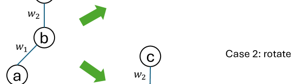
Figure 3: An illustration of the Promote algorithm.

The Promote operation is an important building block to both the correctness and the efficiency of AM-tree. In the next sections, we will discuss efficient algorithms for AM-trees. We first show a strict version of AM-tree in Sec. 4, which always keeps the tree height in $O(\log n)$. However the strict version requires maintaining the child pointers for all nodes, which brings up performance overhead in practice. To tackle this, in Sec.˜5 we discuss the lazy version of the AM-tree, which only requires keeping the parent pointer of each node. By avoiding maintaining child pointers, the lazy version is much simpler, more practical, and easier to program.

4 The Strict AM-tree

In this section, we present the strict AM-tree, where all tree nodes strictly follow the AM-rule at all time. Recall that an AM-tree $T$ supports the following operations: Insert$(u,v,w)$, which updates the tree to reflect an edge insertion $(u,v,w)$ to the graph, ReportMST, which reports information of the current MST, and PathMax$(u,v)$, which gives the maximum edge weight between $u$ and $v$ on the MST.

Among them, we only need to design the algorithm for Insert$(u,v,w)$ that maintains the tree invariants, since PathMax and ReportMST are read-only. We show two solutions to approach this. The first solution is based on a helper function Perch, and is algorithmically simpler. At a high level, it uses the Perch function to promote both $u$ and $v$ to the top of the tree, and then connects $u$ and $v$ with weight $w$, if $w$ is smaller than the current edge between $u$ and $v$. The second approach is based on stitching the paths from $u$ and $v$ to the root without affecting the PathMax results, which is slightly more complicated but practically faster. Both algorithms achieve the same theoretical guarantees. In Sec.˜5, we will extend both of them to lazy versions.

4.1 The High-Level Algorithmic Framework

We start with the high-level framework of AM-tree, presented in Alg. 1. We will analyze the algorithms in Sec. 4.4 and 4.5.

Edge Insertion.   The strict AM-tree rebalances the tree immediately once it is updated. To insert an edge $(u,v,w)$ into an AM-tree $T$, the algorithm starts with a function Link$(u,v,w)$, which applies the edge insertion $(u,v,w)$ such that the tree remains valid, but may be unbalanced. Such an operation may insert the new edge to $T$, or cause an existing edge on $T$ to be replaced by the new edge $(u,v,w)$, or may take no effect to the tree if the new edge $(u,v,w)$ does not appear in the MST of the graph. The resulting tree is not unique—one can use multiple ways to apply Link. We present two algorithms for Link: the first one (Sec. 4.2) is based on a primitive Perch, which is conceptually simpler; the other one (Sec. 4.3) is based on a primitive Stitch, which is more complicated but more efficient in practice. We prove the correctness of the algorithm formally in Thm. 4.1.

The structural changes in the Link operation may cause the tree unbalanced. We say a node $y$ is affected (or may become unbalanced) during the Link operation if either $y$’s children list is changed, or the subtree size of any $y$’s child is changed. We will show that all such nodes are on the path from $u$ or $v$ to the root before the Link operation. We collect all these nodes in a set $S$. Next, a DownwardCalibrate function is applied on each node $y$ in $S$. DownwardCalibrate$(y)$ aims to ensure that node $y$ achieves a balance with all its children. This operation first identifies whether $y$ has a heavy child $x$. If so, $x$ will be promoted and removed from $y$’s subtree. This process is repeated until $y$ is balanced. In Thm. 4.2, we prove that the tree becomes balanced after the Insert operation.

We note that, to perform DownwardCalibrate, we require to store the child pointers in each node, and efficiently determine whether the anti-monopoly rule is violated. To help the reader understand the high-level idea more easily, we assume a black box that can determine whether there is a heavy child of a tree node $u$ (and find it in case so) with $O(1)$ time. Throughout the description and analysis, we assume the existence of this black box, and we give a possible implementation in Sec.˜A.

Path-max Queries.   A PathMax query finds the maximum edge on the path between $u$ and $v$ on $T$. Relevant edges can be identified by first finding Least Common Ancestor (LCA) of $u$ and $v$ as $l$, and finding all edges from $u$ and $v$ to $l$.

Other Queries.   Other MST-related information can be easily maintained during updates. For example, we can easily modify the insertion function to maintain the membership of each edge in the MST. We can use a boolean flag for each edge to denote if it is in the MST. Note that an insertion can only cause one edge to alter in the MST. In Link, when inserting an edge $e$ incurs a replacement of another edge $e^{\prime}$, we can directly change the boolean flag of both edges in $O(1)$ extra cost. Similarly, one can update the total weight of the MST after each insertion in $O(1)$ cost, or maintain an ordered-set of the edges in the MST in $O(\log n)$ cost.

4.2 perch-based Solution

We now present the first implementation of the Link algorithm using the helper function Perch. We call this algorithm linkByperch and present the pseudocode on Lines 1 to 1 in Alg. 1.

To insert an edge $(u,v,w)$ into the graph, we may need to update the AM-tree $T$ accordingly such that it is still a valid transformed MST. Based on the properties of MST, if $u$ and $v$ were not connected before the insertion, the new edge $(u,v,w)$ should just appear in the MST. Otherwise, if $u$ and $v$ were previously connected, the MST may be changed due to the new edge insertion. In particular, adding edge $(u,v,w)$ may introduce a cycle on the graph, and the largest edge on the cycle should be removed. The AM-tree needs to be updated to reflect such a change in the true MST.

The linkByperch$(u,v,w)$ algorithm starts by calling a helper function, Perch, on both $u$ and $v$. The goal of Perch$(x)$ is to restructure the tree and put node $x$ to the top. It simply applies Promote on $x$, until $x$ becomes the root of the tree. Based on Fact˜3.2, the resulting tree is still a valid T-MST, but the tree height may be affected.

After calling Perch on both $u$ and $v$, if $u$ and $v$ were originally disconnected, Perch will make both of them the root of their own tree in the spanning forest. Therefore, we directly attach $u$ to be $v$’s child with the new edge weight $w$.

If $u$ and $v$ were already connected before the edge insertion, the first Perch on $u$ will reroot the tree at $u$, and the second Perch on $v$ will further put $v$ on the top, pushing $u$ down as the child of $v$. In this case, we simply check the current edge weight between $u$ and $v$ (stored in $\mathit{weight}[u]$), and update it to $w$ if $w$ provides a lower value.

Intuitively, the two Perch operations preserve the validity of the T-MST before the edge insertion, and then the new edge is directly reflected on $T$ by connecting $u$ and $v$ by weight $w$. If $u$ and $v$ were connected before, after perching both $u$ and $v$, $u$ and $v$ should be connected by another edge $(u,v,w^{\prime})$. Note that the design of Promote preserves the path-max queries. Hence, since the edge $(u,v,w^{\prime})$ is the only edge from $u$ and $v$ on $T$, $w^{\prime}$ is the path-max. Therefore, if $w<w^{\prime}$, we replace the old edge with the new edge with weight $w<w^{\prime}$.

1

// We omit the maintenance of the $\mathit{size}[\cdot]$ array for simplicity

2

3Function Insert($u,v,w$) // Add an edge $(u,v,w)$

4    $S\leftarrow\{u,v\}\cup\{\text{all ancestors of }u\}\cup\{\text{all ancestors of }v\}$

5    Link$(u,v,w)$ // Plug in linkByperch or linkBystitch

6    foreach node $y\in S$ do  DownwardCalibrate$(y)$

7   

8Function DownwardCalibrate($y$)

9    while $y$ has a child $x$ such that $\mathit{size}[x]>\frac{2}{3}\mathit{size}[y]$ do

10       $\textsf{Promote}(x)$

11      

12Function PathMax$(u,v)$

13    return the maximum edge weight along the path from $u$ to $v$

14   

15

// Perch-based Link function

16

17Function linkByperch$(u,v,w)$

18    Perch$(u)$

19    Perch$(v)$

20    if $\mathit{parent}[u]=v$ then

21       $\mathit{weight}[u]\leftarrow\min(\mathit{weight}[u],w)$

22   else  // $u$ and $v$ were previously disconnected

23       $\mathit{parent}[u]\leftarrow v$

24       $\mathit{weight}[u]\leftarrow w$

25      

26Function $\textsf{Perch}(x)$

27    while $\mathit{parent}[x]\neq$ null do  $\textsf{Promote}(x)$

28   

29

// Stitch-based Link function

30

31Function linkBystitch$(u,v,w)$

32    if $u=v$ or $u=$ null or $v=$ null then

33      return

34   else if $\mathit{parent}[u]\neq$ null and $w>\mathit{weight}[u]$ then

35      linkBystitch$(\mathit{parent}[u],v,w)$

36   else if $\mathit{parent}[v]\neq$ null and $w>\mathit{weight}[v]$ then

37      linkBystitch$(u,\mathit{parent}[v],w)$

38   else

39       if $\mathit{size}[u]>\mathit{size}[v]$ then swap$(u,v)$

40       $u^{\prime}\leftarrow\mathit{parent}[u]$

41       $w^{\prime}\leftarrow\mathit{weight}[u]$

42       $\mathit{parent}[u]\leftarrow v$

43       $\mathit{weight}[u]\leftarrow w$

44       linkBystitch$(u^{\prime},v,w^{\prime})$

45      

Algorithm 1 The Strict AM-tree

4.3 stitch-based Solution

We now present the second solution based on the idea of stitching the tree paths from both $u$ and $v$ to the root. The pseudocode is presented on Lines 1 to 1, and an illustration is shown in 4. Instead of relying on Promote, this approach directly adds the edge $(u,v,w)$ (for an insertion) to the tree, and uses TW transformation to move this edge to its final destination and accordingly restructure the tree. Hence, this approach is slightly less intuitive, but performs faster in practice since it can touch fewer vertices in this process.

Based on TW transformation, if $\mathit{weight}[u]<w$, we can replace the edge with $(\mathit{parent}[u],v,w)$, and recursively call linkBystitch$(\mathit{parent}[u],v,w)$. We do the same thing for $v$. When this process ends (Line 1), the recursive call must have reached two vertices $u$ and $v$ such that $\mathit{weight}[u]>w$ and $\mathit{weight}[v]>w$. To connect $u$ and $v$ with edge weight $w$, we attach the one with smaller subtree size as a child to the larger one. Later in the analysis we will show that this is important to bound the amortized cost of this algorithm. WLOG we assume $\mathit{size}[u]<\mathit{size}[v]$ (swap them otherwise). In this case, we will reassign the parent of $u$ to be $v$ with edge weight $w$.

By doing this, on the current tree $T$, $u$ is connected to both its original parent $u^{\prime}$ and its new parent $v$. Let the weight of the original edge connecting $u$ and $u^{\prime}$ be $w^{\prime}$. Then this edge $(u,u^{\prime},w^{\prime})$ is not a valid tree edge anymore, and we will need to relocate it in the tree. Consider the two edges $(u,u^{\prime},w^{\prime})$ and $(u,v,w)$. Since $w^{\prime}>w$, based on TW transformation, we can equivalently move $(u,u^{\prime},w^{\prime})$ to $(u^{\prime},v,w^{\prime})$. Therefore, the algorithm finally recursively calls linkBystitch$(u^{\prime},v,w^{\prime})$ to finish the process.

Finally, the algorithm has two base cases. The first case is when $u$ and $v$ were connected before. Then by moving edges up, $u$ and $v$ in the recursive calls will finally move to their LCA in the tree and become the same node. In that case, we do not need to further connect them and can directly terminate. The second case is when they were not in the same tree. Then by the recursive calls, one of them will reach the root of the tree, and the parent in the recursive call becomes null. In that case, the algorithm can also terminate directly, since one of the trees has been fully attached to the other.

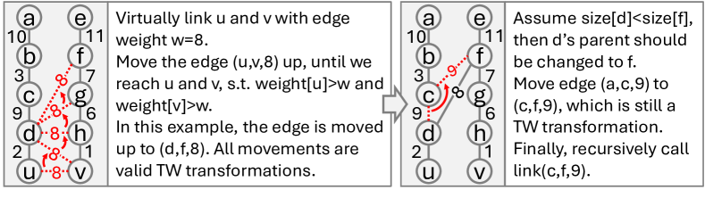
Figure 4: An example of linkBystitch. The figure illusrates linkBystitch$(u,v,8)$. Values on the edges are edge weights. The figure shows all vertices on the path from $u$ and $v$ to the root, and omits all other vertices. An explanation about the process is shown in the figure, and the pseudocode is presented in Alg. 1 Lines 1-1.

4.4 Correctness Analysis

We first show that the correctness of the algorithm, i.e., after the insertion algorithm, the tree 1) is a valid T-MST that handles the insertion of edge $(u,v,w)$ to the original graph, and 2) satisfies the AM rule.

Theorem 4.1 (Correctness)

Given a graph $G=(V,E)$ and a T-MST $T=(V,E_{T})$ for $G$, after Insert$(u,v,w)$ in Alg. 1, using either linkByperch or linkBystitch, $T$ is a valid T-MST for $G^{\prime}=(V,E\cup\{(u,v,w)\})$.

• To show correctness, we need to verify that the path-max query on any two vertices are still preserved. Note that all modifications in DownwardCalibrate only use Promote, which are all TW transformations and preserve the path-max results. Therefore, we only need to show that both linkByperch and linkBystitch preserve path-max results.

  Consider we directly add edge $(u,v,w)$ on $T$, and get a graph $T^{\prime}=(V,E_{T}\cup\{(u,v,w)\})$. Assume we apply the same Link algorithm on $T$ to $T^{\prime}$. Then all path-max queries on $T^{\prime}$ should be the same with that on $G^{\prime}$, and therefore $T^{\prime}$ is PM-equivalent to $G$. We will show that the final result $T$ is PM-equivalent to $T^{\prime}$. Note that $T^{\prime}$ may or may not be a tree, depending on whether $u$ and $v$ were connected before.

  For linkByperch, $T^{\prime}$ is exactly the tree obtained after Line 1 augmented with an additional edge $(u,v,w)$. The final step is the if-conditions from Line 1. In the first case where $u$ and $v$ were not connected before, $u$ is set as the child of $v$ with weight $w$, obtaining a tree $T$ that is the same as $T^{\prime}$. In the second case, $u$ and $v$ were in the same tree. Therefore after the two Perch operations, $u$ should be connected with $v$ with an existing edge $(u,v,w^{\prime})$, and $T^{\prime}$ further augments an edge $(u,v,w)$ to $T$. In this case, only the lower weight should be kept in the MST, and therefore the algorithm selects the minimum of the original weight $w^{\prime}$ and the new weight $w$.

  For linkBystitch, the algorithm exactly first augments $T$ with the virtual edge and get $T^{\prime}$. All later edge movements are TW transformations, as discussed in Sec. 4.3. Therefore, during linkBystitch, $T$ is always PM-equivalent to $T^{\prime}$. The only exception is the base case where $u=v$, the edge with weight $w$ will be dropped in $T$. In this case, conceptually this edge in $T^{\prime}$ is a self-loop on node $u=v$. Therefore, omitting it does not change results for path-max queries.          

We then present the theorem below, which states that the tree stays balanced after insertion. Due to page limit, we defer the proof to Appendix B. The key proof idea is to verify that DownwardCalibrate$(b)$ will always fix the imbalance at node $b$, without introducing other unbalanced nodes. Therefore, calling DownwardCalibrate on all affected nodes in the previous process guarantees to rebalance the tree.

Theorem 4.2 (Balance Guarantee)

After each Insert operation, all nodes in the AM-tree are balanced, and the AM-tree has $O(\log n)$ height.

4.5 Cost Analysis

We now prove the cost bounds for the strict AM-tree. Let $d(\cdot)$ be the depth of a node. We first show the worst-case cost of the two Link functions.

Lemma 4.1

The worst-case cost of linkByperch or linkBystitch is $O(d(u)+d(v))$.

• The simpler case is linkBystitch. In each recursive call, the algorithm reassigns $u$ or $v$ to another node on a higher level. So the worst-case cost is trivially $O(d(u)+d(v))$.

  For linkByperch, we first show that after Perch$(u)$, the depth of any node can increase by at most 1. Perch$(u)$ performs a series of Promote operations on $u$. In a Promote call, let $y$ be the parent of $u$. Only the nodes in $y$’s subtree may have their depth increased by 1 (see the rotate case in Fig.˜3). After that, $u$ is promoted one level up, and $y$ can never be the parent of $u$ again. Therefore, the depth of any node can be increased by at most 1.

  In linkByperch, we perch both $u$ and $v$ and then connect $u$ and $v$. The latter part takes constant time, so we only need to consider the cost of perching $u$ and $v$. The function Perch$(u)$ performs $d(u)$ calls to Promote($u$), each of which decreases $d(u)$ by 1. So Perch$(u)$ takes $O(d(u))$ time. After perching $u$, the depth of $v$ is increased by at most 1. Therefore, Perch$(v)$ takes $O(d(v))$ time. Combining all the above, the worst-case cost for linkByperch is $O(d(u)+d(v))$.          

We then show that the worst-case cost for Insert is $O(\log^{2}n)$. Due to page limit, we defer the proof in Appendix C. The key idea is that, since both $d(u)$ and $d(v)$ are $O(\log n)$ (Thm. 4.2), there are at most $O(\log n)$ nodes accessed by Perch and to be calibrated at the end, each of them can be recalibrated for $O(\log n)$ times.

Theorem 4.3

The worst-case cost for Insert is $O(\log^{2}n)$.

Next, we use amortized analysis to show that the Insert and PathMax operations take $O(\log n)$ amortized time. We define the potential function for a node $u$ as:

(4.1) $$\phi(u)=\log\mathit{size}[u]$$

We also define the potential function for the whole tree as:

(4.2) $$\Phi(T)=\sum_{i=1}^{n}\phi(i)=\sum_{i=1}^{n}\log\mathit{size}[i]$$

It is obvious that the potential function is always non-negative, and the potential of the whole is $O(n\log n)$. Recall that the amortized cost for an operation $\mathit{op}$ is $\mathit{C}_{\mathit{amortized}}(\mathit{op})=\mathit{C}_{\mathit{actual}}(\mathit{op})+\Delta(\Phi(T))$, where $\mathit{C}_{\mathit{actual}}(\mathit{op})$ is the actual cost (number of instructions) in the operation $\mathit{op}$, and $\Delta(\Phi(T))$ is the change of potential function on tree $T$ after the operation. We first prove the following important lemma, which states that, if a promotion is performed due to imbalance, the amortized cost of Promote is free. In other words, the cost of the Promote can be fully charged to previous operations that increase the potential of the tree.

Lemma 4.2

If $\mathit{size}[x]>(2/3)\cdot\mathit{size}[\mathit{parent}[x]]$, the operation Promote$(x)$ has zero amortized cost.

• We first show that in both the rotate and the shortcut case, the potential of the tree will decrease by at least 1. Let $y=\mathit{parent}[x]$. Note that during Promote($x$), only the potential for $x$ and $y$ will change.

  Let $s(\cdot)$ be the size of a node before Promote, and $s^{\prime}(\cdot)$ the size after. Based on the assumption in the lemma, $s(x)>(2/3)s(y)$. In a shortcut case, $x$’s potential remains unchanged, and the size of $y$ decreases by at least a factor of $2/3$, causing its potential to decrease by $\log_{2}3>1$. In a rotate case, $s^{\prime}(x)=s(y)$. For $y$, we have $s^{\prime}(y)=s(y)-s(x)<(1/2)s(x)$. The potential change after a Promote is $(\log s^{\prime}(x)+\log s^{\prime}(y))-(\log s(x)+\log s(y))<\log s(y)+\log(1/2)s(x)-\log s(x)-\log s(y)=-1$. Combining the actual cost and the potential change, Promote$(x)$ has zero amortized cost when $\mathit{size}[x]>(2/3)\mathit{size}[\mathit{parent}[x]]$.

  Suppose the actual cost of Promote$(x)$ is a constant $c$. If we use potential function $\phi^{\prime}(x)=c\cdot\log\mathit{size}[x]$, we will have $\mathit{C}_{\mathit{amortized}}(\mathit{op})=\mathit{C}_{\mathit{actual}}(\mathit{op})+\Delta(\Phi(T))=k+(-k)=0$. Thus, the operation Promote$(x)$ has zero amortized cost if $\mathit{size}[x]>(2/3)\cdot\mathit{size}[\mathit{parent}[x]]$.          

From Lemma˜4.2, we have the following conclusion.

Lemma 4.3

Assume identifying the heavy child of a node has $O(1)$ cost. Then DownwardCalibrate has $O(1)$ amortized cost.

• The DownwardCalibrate operation is a sequence of Promote operations on a node $x$ such that $\mathit{size}[x]>(2/3)\mathit{size}[\mathit{parent}[x]]$. Based on Lemma˜4.2, all Promote operations have zero amortized cost. Hence, the amortized cost for DownwardCalibrate is $O(1)$.          

We now show the amortized cost of the linkByperch and linkBystitch, which will be used to prove Thm. 4.5.

Lemma 4.4

The linkByperch$(u,v,w)$ operation has $O(d(u)+d(v)+\log n)$ amortized cost.

• By Lemma˜4.1, the actual cost of linkByperch is $O(d(u)+d(v))$. We then prove that the increment of the potential is $O(\log n)$. The linkByperch function has three steps: two Perch function calls and the final step to link $u$ and $v$. In the two Perch calls, we repeatedly promote $u$ or $v$ to a higher level. For both shortcut and rotate cases, the sizes of all other nodes are non-increasing, so only $\phi(u)$ and $\phi(v)$ may increase. In the last step, when connecting $u$ and $v$, the only case that may cause the potential change is when a new edge is established, $u$ becomes a child of $v$, and only $\phi(v)$ may increase. Combining all the steps, the only increment on the potential function is $\phi(u)$ and $\phi(v)$, so the increment of the potential function is at most $O(\log n)$.          

Lemma 4.5

The linkBystitch$(u,v,w)$ operation has $O(d(u)+d(v))$ amortized cost.

• By Lemma˜4.1, the actual cost of linkBystitch is $O(d(u)+d(v))$. For the potential increment, note that the only structure change occurs on lines 1 and 1. Since we always attach the smaller subtree to the larger one, $\mathit{size}[v]$ can increase by at most twice, increasing $\phi(v)$ by at most 1. Since there are at most $O(d(u)+d(v))$ nodes affected in the algorithm, the potential change is also $O(d(u)+d(v))$.          

In a size-balanced tree, $d(u)$ and $d(v)$ are $O(\log n)$. Combining Fact 3.1, Lemmas 4.3, 4.4, and 4.5, we have the following theorem for the entire Insert function.

Theorem 4.4

The amortized cost for each Insert is $O(\log n)$ using either linkByperch or linkBystitch.

The bound of the PathMax$(u,v)$ query is trivially $O(\log n)$ since the tree height is $O(\log n)$. We can find the lowest common ancestor (LCA) and compare all edges on the path between $u$ and $v$. To summarize, we have the following theorem on the cost bounds for the strict AM-tree.

Theorem 4.5

The strict AM-tree supports PathMax in $O(\log n)$ worst-case cost, and Insert in $O(\log n)$ amortized cost ($O(\log^{2}n)$ worst-case cost).

4.6 Finding Heavy Child of a Node

As mentioned, the strict AM-tree requires a building block to identify the heavy child (if any) of a given node. This requires maintaining all child pointers in each node, and maintaining the heaviest child under possible changes to the tree structure. For page limit, we present the algorithm for this part in Appendix A.

5 The Lazy AM-tree

In Sec. 4, we introduced the strict version of AM-tree, which always keeps the tree size-balanced. However, this version requires maintaining all the child pointers in each node and the building block in Appendix A to identify the heavy child, which may bring up unnecessary performance overhead.

In this section, we introduce a lazy version of AM-tree, which only requires each tree node to maintain the parent pointer. This version rebalances the tree lazily, so the tree height is not always bounded by $O(\log n)$. However, we will show that the lazy AM-tree also achieves the same $O(\log n)$ amortized cost for insertions and path-max queries.

5.1 Algorithms

We present the algorithm in Alg. 2. This algorithm still uses the two primitives: Link, which is the same as the strict version, and UpwardCalibrate. Different from DownwardCalibrate in the strict version, which rebalances a node with its children, the UpwardCalibrate function tries to rebalance a node with its parent. In particular, UpwardCalibrate$(u)$ will check the path from $u$ to the root and guarantee that any two of $u$’s consecutive ancestors $x$ and $y=\mathit{parent}[x]$ satisfies $\mathit{size}[x]\leq(2/3)\cdot\mathit{size}[y]$. As such, the depth of $u$ is reset to $O(\log n)$. To do this, UpwardCalibrate$(x)$ repeatedly promotes $x$ if $x$ is a heavy child of its parent (i.e., its size is more than $2/3$ of its parent). When $x$ is no longer a heavy child, we move to its parent and continue.

Using UpwardCalibrate, we can balance the tree in a lazy way. The algorithm also becomes much simpler. In LazyPathMax$(u,v)$, we first call UpwardCalibrate on both $u$ and $v$ to calibrate the path from each of them to the root. Then we directly use the plain algorithm to find all edges on the path and obtain the maximum one.

In LazyInsert$(u,v,w)$, we also first use UpwardCalibrate on both $u$ and $v$ to calibrate the path from each of them to the root. Then we use the same linkByperch or linkBystitch functions to connect $u$ and $v$ as in the strict version, and connect them by an edge with weight $w$ (modifying other edges of the tree if necessary). The algorithm does not then calibrate the tree after Link. For this reason, the tree after a LazyInsert is not guaranteed to be size-balanced. The rebalance process will be postponed to the next time when a node is accessed in either an insertion or a path-max query.

In the next section, we will show that, although the tree is not guaranteed to be balanced, the amortized costs for both LazyInsert and LazyPathMax are still $O(\log n)$.

1

2Function LazyInsert$(u,v,w)$

3    UpwardCalibrate$(u)$

4    UpwardCalibrate$(v)$

5    Link$(u,v,w)$ // plug in linkByperch or linkBystitch in Alg. 1

6Function LazyPathMax$(u,v)$

7    UpwardCalibrate$(u)$

8    UpwardCalibrate$(v)$

9    return PathMax$(u,v)$ // See Alg. 1

10Function UpwardCalibrate$(x)$

11    while $\mathit{parent}[x]$ is not null do

12       while $\mathit{size}[x]>\frac{2}{3}\mathit{size}[\mathit{parent}[x]]$ do  promote$(x)$

13       $x\leftarrow\mathit{parent}[x]$

14      

Algorithm 2 The Lazy AM-tree

5.2 Analysis

We now analyze the lazy AM-tree. We use the same potential function as in the strict version. We first note that the correctness of the lazy version can be directly derived from the same proof for the strict version (Thm. 4.1), and the following theorem holds.

Theorem 5.1 (Correctness of the Lazy AM-tree)

Given a graph $G=(V,E)$ and a T-MST $T=(V,E_{T})$ for $G$, after the LazyInsert$(u,v,w)$ in Alg. 2 using either linkByperch or linkBystitch, $T$ is a valid T-MST for $G^{\prime}=(V,E\cup\{(u,v,w)\})$.

We now analyze the amortized cost. The UpwardCalibrate$(x)$ function will not fully calibrate the tree, but it will calibrate the path from $x$ to the root to ensure the depth of $x$ becomes $O(\log n)$, as stated in the following lemma.

Lemma 5.1

After UpwardCalibrate on $u$ and $v$, the depth of $u$ and $v$ becomes $O(\log n)$.

• UpwardCalibrate$(x)$ will make all nodes on the path from $x$ to the root to be size-balanced, so the depth of $u$ and then $v$ will be adjusted to $O(\log n)$.

  However, the second UpwardCalibrate on $v$ may change the depth of $u$. Similar to the proof of Lemma˜4.1, we can also show that UpwardCalibrate$(v)$ will increase the depth of any node by at most 1. UpwardCalibrate$(v)$ performs a series of Promote operations on $v$ or $v$’s ancestors. Let $x$ be the node being promoted and $y$ be the parent of $x$, then the depth of nodes in $y$’s subtree may increase by 1 (see the rotate case in Fig.˜3). After that promote, $x$ is brought one level up, and the node being promoted in future can only be $x$’s ancestors, so $y$ can never be the parent of the node being promoted again. Therefore, the depth of any node can be increased by at most 1. Thus, both $u$ and $v$ have depth $O(\log n)$ after UpwardCalibrate on $u$ and $v$.          

We then show that the UpwardCalibrate function itself only has $O(\log n)$ amortized cost. Note that since UpwardCalibrate may work on an unbalanced tree, it may access $\Omega(\log n)$ nodes on the path, resulting in an $\Omega(\log n)$ actual cost. However, since some of the operations, specifically the Promote operations, rebalance the tree and decrement the potential function, the amortized cost can be bounded in $O(\log n)$.

Lemma 5.2

The UpwardCalibrate operation has $O(\log n)$ amortized cost.

• First of all, note that the Promote function in the inner while-loop on Line 2 is performed only if imbalance occurs. In Lemma 4.2, we proved that this operation has zero amortized cost, since it decrements the potential function. Therefore, the entire while-loop on Line 2 has $O(1)$ amortized cost, indicating that each iteration of the outer while-loop on Line 2 only has $O(1)$ amortized cost.

  We then prove that the outer while-loop has $O(\log n)$ iterations. This is because in each iteration, when the inner loop terminates, we must have $\mathit{size}[x]\leq\frac{2}{3}\mathit{size}[\mathit{parent}[x]]$. Then we update $x$ to its parent and continue to the next iteration. Therefore, each iteration increases the size of the current node $x$ by at least a factor of $3/2$. In at most $O(\log n)$ iterations, the outer while-loop terminates.          

Combining the above lemmas and the amortized cost of linkByperch and linkBystitch proved in Lemma 4.4 and 4.5, we have the following theorem.

Theorem 5.2

The lazy AM-tree supports the LazyInsert and LazyPathMax in $O(\log n)$ amortized time per operation.

6 Persisting the AM-tree

We now discuss how to persist AM-tree upon updates, which is required in certain temporal graph applications. Since we focus on temporal graphs, we mainly consider partial persistence, where updates are applied only to the last version but we can query any history version. The methodology here also extend to the fully persistent setting where all versions form a DAG instead of a chain.

To persist the AM-tree, we only need to persist the arrays for $\mathit{parent}[\cdot]$ and $\mathit{weight}[\cdot]$. Below we just use the $\mathit{parent}[\cdot]$ as an example. Assume there are $m=\Omega(\log n)$ edge insertions to AM-tree. Let $k$ be the total number of nodes that are modified by the $m$ edge insertions. The analysis in Sec. 4.5 and 5.2 shows that $k=O(m\log n)$.

Version Lists.   We first consider a simple and practical solution based on version lists (referred to as “fat nodes method” in [16]). All experiments in this paper use this approach. For this approach, each node $u$ in the AM-tree maintains a list of versions of $\mathit{parent}[u]$, which consists of pairs of $(t,\mathit{parent}_{t}[u])$ ordered by $t$, where $t$ is the time when the edge is added, and $\mathit{parent}_{t}[u]$ is the parent of $u$ in this version. When the parent of $u$ is updated, a new pair of $(t,\mathit{parent}[u]_{t})$ is appended to the version list. In this case, no asymptotic cost is needed for supporting persistent insertions. and the version lists take $O(k)=O(m\log n)$ space. However, when querying a history version, we need a binary search to locate the pointers of the current version, which adds an $O(\log k)=O(\log m)$ overhead to query costs.

Note that, only the strict AM-tree can guarantee the $O(\log m\log n)$ query cost, where PathMax will check $O(\log n)$ edges in the tree. The query cost for the lazy AM-tree is amortized; however, in practice, the difference in query performance between the two versions is minimal.

vEB-Trees-based Solution.   Theoretically, the overhead for persistence can be reduced from $O(\log m)$ to $O(\log\log m)$ by using the approach given in Straka [49]. At a high level, the ordered set is maintained by a van Embe Boas Tree [55] that provides doubly logarithmic update and lookup cost.

7 Applications on Temporal Graphs

With the algorithms for AM-tree with support for persistence, we are ready to solve various temporal graph applications. In Sec.˜2.2, we briefly introduced the point-interval temporal connectivity problem. In this section we show other temporal graph problems and how AM-trees can solve them. We first review the temporal graph settings.

7.1 Temporal Graph Settings

Two categories in temporal graph processing have received significant attention. The first is the point-interval setting (e.g., [11, 34, 5, 12, 48, 54, 57, 58, 60, 59, 61]) as mentioned in Sec.˜2.2. In this setting, each edge $e$ has a timestamp $t(e)$ (i.e., edge $(u,v)$ arrives at time $t(e)$). A query is associated with a time interval $[t_{1},t_{2}]$ and is performed on a sub-graph $G^{\prime}_{[t_{1},t_{2}]}$ with edge set $E^{\prime}=\{e~|~t(e)\in[t_{1},t_{2}]\}$. A simpler case is the so-called sliding-window setting [5, 12].

Dually, there is the interval-point setting (e.g., [19, 13, 41, 17, 24, 44, 6]), where each edge $e$ has a time interval $[t_{1}(e),t_{2}(e)]$. A query is associated with a timestamp $t$ and is performed on the sub-graph $G^{\prime}_{t}$ with edge set $E^{\prime}=\{e~|~t\in[t_{1}(e),t_{2}(e)]\}$. A similar setting is the “offline dynamic graphs” [41, 17], where each edge can be inserted/deleted at a certain time, and queries are performed on a snapshot of the graph. From a temporal view, each edge has a lifespan (an interval) from its insertion to its deletion, and queries are performed on a specific timestamp. However, in fully dynamic graphs [20, 39, 21, 7, 53, 22, 36, 35], the deletion time is unknown at the time of insertion.

7.2 Online/Offline Settings

The graph and queries can also be either online or offline. Offline means the information is known ahead of time, while online means the algorithm needs to respond to every update/query before the next one comes. We first consider the graph:

• Offline Graph [54, 57, 58, 60, 59, 41, 17]: all edges in the graph are known ahead of time (before or with the queries).

• (Online) Streaming Graph [5, 12, 48, 54, 61]: New edges arrive one by one, forming a graph stream. In this case, the timestamp of the edge is the ordering of it in the stream, so only the point-interval setting applies here.

AM-tree can solve the online version of incremental MST. An offline setting can be converted to online by sorting all edges based on the time and processing them.

The queries can also come in different settings:

• Offline Queries [48, 5, 12, 60, 61]: All queries are known ahead of time.

• (Online) Historical Queries [54, 57, 58, 60, 59, 41, 17]: Queries come as a stream, and can travel back in history to query any previous timestamp or time interval. This requires to persist the graph (or the corresponding data structure).

In summary, there are a variety of different temporal graph settings, and they have been studied either within the temporal graph scope or as other problems (e.g., offline dynamic graphs [41, 17]). However, even though the literature has designed solutions for some specific settings, one contribution of our work is to show how a base data structure can be adapted to different settings. In particular, the AM-tree, which supports efficient incremental MST, can be used for a wide range of problems (mostly connectivity-related problems) in this section, combined with all the settings discussed above. Next, we will use connectivity as the main example, and show two other problems that can also be solved with some moderate modifications. For page limit, more applications are discussed in Sec.˜D. For many applications, their reductions to MST-related problems have been studied in a specific graph-query setting [5, 12]. Our discussions show that they can all be solved by AM-trees and can be extended to other settings in a straightforward way.

7.3 Connectivity

On an undirected graph $G=(V,E)$ there are two crucial problems related to graph connectivity:

• Determine whether $u$ and $v$ are connected in $G$.

• Report the number of connected components in $G$.

In temporal graph applications, the graph contains edges with temporal information. We show that both the point-interval and the interval-point settings can be converted to incremental MST and solved by AM-trees efficiently.

The point interval setting is discussed in Sec.˜2.2 as a motivating example, and we briefly recap here. Each edge $e$ is treated as an edge insertion at time $t(e)$ with weight $-t(e)$. We can then maintain an AM-tree by processing all edges in order as an incremental MST. We use $T_{t}$ to denote the AM-tree up to time $t$. For a query $(u,v,t_{1},t_{2})$, we check and report if the $\textsf{PathMax}{}_{T_{t_{2}}}(u,v)=w$ satisfies $|w|\geq t_{1}$ [12, 5, 48]. To report the number of connected components (CC) [12], note that all edges $e$ in $T_{t_{2}}$ with $t(e)<t_{1}$ break the connectivity of the graph and increase the number of CCs by 1. We keep an ordered set $D$ to store all edges in the MST, ordered by $t(e)$. For each edge insertion to the MST, we update the active edges in $D$ (up to one edge inserted/removed). For a query $(t_{1},t_{2})$, we look at $D_{t_{2}}$ ($D$ at time up to $t_{2}$), and report $n-|\{e~|~t(e)\geq t_{1}\}|$. $D$ can be maintained by any balanced BST in $O(\log n)$ cost per insertion, deletion, or query.

For the interval-point setting, each edge has a time interval $[t_{1}(e),t_{2}(e)]$. We convert it to an incremental MST problem by adding this edge at time $t_{1}(e)$ with weight $-t_{2}(e)$. Again we use $T_{t}$ to denote the AM-tree up to time $t$. For a query $(u,v,t)$, we query $w=\textsf{PathMax}{}_{T_{t}}(u,v)$ on $T_{t}$ and check whether $|w|\geq t$. If so, $u$ and $v$ remain connected at time $t$. We can similarly use AM-tree to answer the number of connected components queries.

Note that we need to perform the PathMax (or check BSTs for the number of CCs) for each query. If the queries are offline, we can sort the query time ($t$ or $t_{2}$) together with the edges, so all PathMax applies to the “current” AM-tree in the stream. For the historical setting, we need to persist the AM-tree (and also the ordered set $D$), so queries can travel back and check any previous version of AM-tree or $D$. We show the theoretical guarantee on this problem along with the following application on bipartiteness in Thm. 7.1.

7.4 Bipartiteness

An undirected graph $G=(V,E)$ is bipartite iff there exist a vertex subset $V^{\prime}\in V$ that every edge has one endpoint in $V$ and the other endpoint in $V\setminus V^{\prime}$.

There is a known reduction [4, 12] of the bipartiteness problem to the connectivity problem. One can check whether a graph $G$ is bipartite using the following approach. We generate $G^{\prime}$ by duplicating each vertex $v\in V$ into two copies $v_{1}$ and $v_{2}$ in $G^{\prime}$, and duplicating each edge $(u,v)\in E$ into $(u_{1},v_{2})$ and $(v_{1},u_{2})$ in $G^{\prime}$. The graph $G$ is bipartite if and only if $G^{\prime}$ has twice connected component as $G$.

Solving bipartiteness checking in the temporal setting is similar to connectivity. We run the same algorithm for connectivity on both $G$ and $G^{\prime}$. For a query at time $t$, we check and return if the number of connected components on $G^{\prime}_{t}$ is twice as $G_{t}$. The same cost analysis for connectivity also applies here. Using vEB tree for persistence leads to the following theorem.

Theorem 7.1

Given a graph with $n$ vertices and $m$ edges, temporal graph on applications of connectivity or bipartiteness can be solved by AM-trees with $O(n)$ initialization cost and $O(\log n)$ cost per edge update; the offline query and historical query have $O(\log n)$ and $O(\log n\log\log m)$ cost, respectively.

Note that in offline cases, we assume $m=\Omega(n)$ since otherwise we can filter out singleton vertices that are not connected to any other vertex.

7.5 $k$-Connectivity and $k$-Certificate

Given an undirected graph $G=(V,E)$, two vertices $u$ and $v$ are $k$-connected if there are $k$ edge-disjoint paths connecting them. A graph is $k$-connected if every pair of vertices is $k$-connected.

A $k$-certificate is a sequence of edge-disjoint spanning forest $F_{1},F_{2},...,F_{k}$ from $G$, and $F_{i}$ is a maximal spanning forest of $G\setminus(F_{1}\cup F_{2}\cup\cdots\cup F_{i-1})$. The connection between the $k$-certificate and $k$-connectivity is that $u$ and $v$ are $k$-connected in $G$ if and only if they are $k$-connected in $(F_{1}\cup F_{2}\cup\cdots\cup F_{i-1})$.

Generating $k$-certificate can rely on using the algorithm for connectivity [12]. $F_{1}$ is simply the same MST computed in Sec.˜7.3 using the AM-tree. Then, when $F_{i}$ is updated—an edge $e$ is replaced by another edge in the MST, it will be inserted into $F_{i+1}$. Hence, in total we maintain $k$ AM-trees, so the cost is multiplied by $k$ (asymptotically the same when assuming $k=O(1)$).

7.6 Other Applications

Due to the space limit, we discuss other applications in Sec.˜D.

8 Experiments

This section provides experimental evaluation of the effectiveness of AM-trees. We mostly focus on one setting, the point-interval temporal connectivity, due to the following reasons. First, there exist fast baselines for this problem [48] that are apple-to-apple comparisons to AM-trees. Second, when mapping to incremental MST, the interval-point setting only changes the edge weight distribution, and the runtime is similar. Additional experiments are in Appendix E.

For the point-interval connectivity, each edge $e$ has a timestamp $t_{e}$. A query is associated with a time interval $[t_{1},t_{2}]$, and only an edge $e$ with a timestamp $t_{e}\in[t_{1},t_{2}]$ are considered in the query. In this section, we mainly focus on querying the connectivity between two vertices. We provide the experiment for querying the number of connected components in Appendix E.3. As discussed in Sec. 7.3, it is an important building block for many temporal applications such as bipartiteness checking. Our source code is publicly available on github [15].

8.1 Setup

We implemented the strict and the lazy versions of AM-tree in C++ and persist them by version lists (see Sec. 6). We ran all experiments on a Linux server with four Intel Xeon Gold 6252 CPUs and 1.5TB main memory. We compiled our code using Clang 18.1 with the -O3 flag.

Datasets   We tested seven real-world graphs (summarized in Tab.˜1) with very different features. The first three graphs are real-world temporal graphs where each edge is associated with a timestamp. The last four are static graphs and we assign a random timestamp to each edge.

Name	Graph	$|V|$	$|E|$
WT	∗wiki-talk [33]	1.1M	7.8M
SX	∗sx-stackoverflow [33]	6.0M	63.5M
SB	∗soc-bitcoin [45]	24.6M	122.4M
USA	RoadUSA [38]	24.0M	57.7M
GL5	GeoLife [62, 56]	24.9M	124.3M
TW	Twitter [32]	41.7M	1.47B
SD	sd_arc [37]	89.2M	2.04B

Table 1: Graph Information. ^∗: real-world temporal graphs. Others are static graphs with randomly generated temporal information.

Evaluated Methods   We compared six data structures in total. For each of them, we test the throughput for both updates (processing all temporal edges) and queries.

• Strict-Stitch, Strict-Perch, Lazy-Stitch, Lazy-Perch: Our implementations of four versions of AM-tree using strict/lazy strategy based on Perch/Stitch.

• OEC-Forest [48]: A state-of-the-art implementation for incremental MST, which solves temporal connectivity.

• LC-Tree: Our own implementation of link/cut trees [47].

Recall that the LC-Tree is a classic data structure offering theoretical guarantees, whereas OEC-Forest is a practical data structure without non-trivial bounds. All four versions of AM-tree provide the same (amortized) bounds as LC-Tree, and are also designed to be practical. For the AM-trees and OEC-Forest we also tested their persistent version for historical queries. We note that, as mentioned in Sec. 6, the lazy AM-trees do not guarantee the $O(\log n\log\log m)$ query bound. The update bounds for the lazy version, and all bounds for the strict versions still hold in the persistent setting.

Figure 5: Update and query throughput (millions of operations per second) for offline queries. Higher is better.

Figure 6: Update and query throughput (millions of operations per second) for online (historical) queries. Higher is better.

8.2 AM-trees for Offline Queries

We first tested the non-persistent AM-tree for offline queries, i.e., the queries are given ahead of time with all edges. In this case, there is no need to persist the AM-tree. We can simply process (insert) the edges in order, and after each insertion, if there is a query that corresponds to this time, we directly perform it. Fig.˜6 shows the update and query throughput in this setting.

Update Throughput.   We first compare among the four versions of AM-tree in updates. The lazy version always achieves much better performance than the strict version, due to two main reasons. First, the lazy version does not maintain the children pointers and does not actively check the heaviest child, which saves much work. Second, the lazy version does not rebalance the tree after update, and thus requires less work than the strict version. In total, the performance for the lazy version is 3.6–6.2$\times$ faster on average on all graphs.

The stitch-based versions are usually slightly faster than the perch-based versions. Such a difference is more pronounced in the persistent settings, which we discuss later.

Compared to other baselines, while LC-Tree achieves strong theoretical guarantee, it has the lowest throughput on all graphs. It is slower than the strict AM-trees by a factor of 1.2–2.6$\times$, and is slower than the lazy AM-trees and OEC-Forest by at least 4.5$\times$. OEC-Forest tree has reasonably good performance on all graphs. The best version of AM-trees, Lazy-Stitch still achieves competitive or better performance than OEC-Forest, which is from 4% slower (on WT) to 1.5$\times$ faster (on SB). On average across seven graphs, Lazy-Stitch is 1.2$\times$ faster. This speedup comes from the theoretical guarantee of the AM-tree that leads to shallower tree depths.

Query Throughput.   For queries, all versions of AM-tree has better performance than both OEC-Forest and LC-Tree. The advantage over LC-Tree is from the algorithmic simplicity, and the advantage over OEC-Forest is from the depth guarantee of AM-tree in theory. To verify this, we further tested the average tree height for AM-tree and OEC-Forest, and present the results in Sec.˜E.1 for completeness. Comparing OEC-Forest with Lazy-Stitch as an example, OEC-Forest is 1.8–2.9$\times$ deeper than AM-tree, making AM-tree 1.6–2.5$\times$ faster than OEC-Forest for queries.

8.3 AM-trees for Historical Queries

We now discuss the setting with historical queries, which requires using the persistent version of AM-trees. In this setting, the queries are not known when the index is constructed, so we need to preserve all versions of the AM-tree at all timestamps. We present the results in Fig.˜6.

The performance for updates is pretty consistent with the non-persistent version. In all cases, Lazy-Stitch achieves the best performance, and OEC-Forest is close to our best performance. For queries, the slowdown of perch-based version over the stitch-based one becomes significant. As mentioned, the difference comes from the more substantial tree restructuring in Perch. linkByperch changes $\Theta(d(u)+d(v))$ nodes in the tree. Note that this bound is tight, since $u$ and $v$ both have to be perched to the top, causing all nodes on the path to generate a new version. For linkBystitch, in many cases, the edge is just conceptually moved up without changing the tree. To verify this, in Sec.˜E.2 we report the number of versions generated during the algorithm, which indicates the total number of nodes that have been touched and changed their parent/child pointers during the entire algorithm. The perch-based algorithms indeed modified 1.4–5.5$\times$ more nodes than the stitch-based versions.

Since the lazy versions have loose query bounds, we observe that the strict version can achieve better performance than the lazy versions. This is more pronounced for the perch-based algorithms. For the stitch-based algorithms, the difference is marginal except for the last graph SD. On all graphs other than SX, both Strict-Stitch and Lazy-Stitch outperforms the baseline OEC-Forest.

In summary, Lazy-Stitch achieves the best overall performance for almost all settings. When the application emphasizes on the query throughput in the online setting, Strict-Stitch may provide better performance in queries.

9 Related Work

Minimum spanning tree/forest (MST/MSF) is one of the most fundamental graph problems, and has been studied from a century ago [27, 8] to recent years [30, 28, 14]. Some famous algorithms include but are not limited to: Borůvka’s algorithm [8], Prim’s algorithm [42, 27], Kruskal’s algorithm [31], and the KKT algorithm [29]. Regarding MSTs with edge updates, the classic dynamic setting (supporting edge insertions and deletions) is challenging—the best-known algorithm [23] needs $O(\log^{4}n/\log\log n)$ amortized cost per edge update. Incremental MST (only supporting edge insertions) is simpler, and proven to be very useful.

Some classic data structures can solve incremental MST efficiently in theory, including the link-cut tree [47], the rake compress tree (RC-tree) [3], and the top tree [52]. They can support each edge insertion in $O(\log n)$ cost either amortized or on average. These data structures actually solve a more general problem called “the dynamic tree/forest” problem (see [2]). One attempt to improve them is introducing parallelism (on a large batch of edge updates) [5, 18, 40, 46]. To the best of our knowledge, these results are mostly of theoretical interest and no implementations are available. Practically, people have designed data structures such as the OEC-forest [48] and the D-tree [10] for faster performance. D-tree maintains a BFS-tree and patches it when updates come. It can have decent performance when the graph has certain properties, but no non-trivial cost bounds can be guaranteed. The OEC-forest [48] was the latest work on this topic and also the main baseline we compare with. The OEC-forest is a T-MST, and it uses an idea similar to our stitch-based algorithms. However, it does not support any non-trivial (better than linear) bounds for the tree diameter and thus the theoretical costs for updates and queries. Our main improvement is to introduce the anti-monopoly rule, which bounds the tree height and guarantees the cost bounds for AM-tree.

Temporal graph processing is a popular research topic recently, and we refer the audience to an excellent survey [25] for more backgrounds. The connection between temporal graph and incremental MST has been shown, but only for specific cases. Song et al. [48] discussed the historical point-interval connectivity, and Anderson et al. [5] discussed the offline point-interval setting. To the best of our knowledge, the generalization of this connection is novel in our paper.

10 Conclusion

In this paper, we propose new algorithms for incremental MST to support efficient temporal graph processing on numerous applications. Our new data structure, the AM-tree, is efficient both in theory and in practice. In theory, the cost bounds of using AM-trees to support temporal graphs match the best-known results using link-cut trees or other data structures. In practice, we compare AM-tree to both the theoretically efficient solution and state-of-the-art practical solutions, and our Lazy-Stitch version achieves the best performance in most experiments including various graphs with offline/historical queries on both updates and queries.

A Finding the Heavy Child of a Node

Recall that in the strict version, we need to efficiently identify the heavy child of a node (if any) in the DownwardCalibrate function. In this section, we discuss possible data structures to implement such queries. The data structure needs to support the following operations:

• AddChild$(x,y)$: Add $x$ as a child of $y$.

• RemoveChild$(x,y)$: Remove $x$ from the children of $y$.

• GetHeavyChild$(y)$: Return the heavy child of $y$, or null if $y$ does not have a heavy child.

To do this, we use bit operations to support constant time cost per operation. For each node $y$, we maintain the following information:

• $L[0..\lfloor\log n\rfloor]$: $\lfloor\log n\rfloor+1$ doubly linked lists. $L[i]$ contains $y$’s children whose subtree size is in the range $[2^{i},2^{i+1})$.

• $\mathit{cnt}[0..\lfloor\log n\rfloor]$: The number of children in each list.

• A integer $w$: the $i$’th bit of $w$ is set to 1 if $cnt[i]>0$.

When adding/removing $x$ as a child of $y$, let $i=\lfloor\log\mathit{size}[x]\rfloor$. We can simply add/remove $x$ to/from the list $L[i]$ of $y$ and update $y$’s $\mathit{cnt}[i]$ and $w$ accordingly.

For GetHeavyChild$(y)$, we can directly return null if $w=0$. Otherwise, we find the high-bit of $w$ as $h$. If $cnt[h]=1$, we get the only child $x$ in $L[h]$. This means that $x$ is the heaviest child of $y$. Therefore, we just need to check whether $\mathit{size}[x]>(2/3)\mathit{size}[y]$ and return the result accordingly.

The most involved case is $cnt[h]>1$, which means $y$ has at least two children with subtree size in $[2^{h},2^{h+1})$. In this case, we directly return null because the heaviest child cannot be greater than $(2/3)\mathit{size}[y]$. To see why, suppose the heaviest two children are $x_{1}$ and $x_{2}$ where $2^{h}\leq\mathit{size}[x_{2}]\leq\mathit{size}[x_{1}]<2^{h+1}$. Then we have $\mathit{size}[x_{2}]/\mathit{size}[x_{1}]>1/2$. Then $\mathit{size}[x_{1}]/\mathit{size}[y]<\mathit{size}[x_{1}]/(\mathit{size}[x_{1}]+\mathit{size}[x_{2}])=1/(1+\mathit{size}[x_{2}]/\mathit{size}[x_{1}])<2/3$. Therefore $x_{1}$ is not the heavy child of $y$, and $y$ does not have a heavy child in this case.

All the above operations trivially have constant time cost except for computing $\lfloor\log\mathit{size}[x]\rfloor$ and taking the high-bit $h$ of $w$. Note that $\mathit{size}[x]\in[1,n]$ and $w\in[0,n]$, so both of the operations can be addressed by preprocessing the results for all values in $[0,n]$. In other words, we can use an array to store the $\lfloor\log k\rfloor$ and the high-bit of $k$ for each integer of $k\in[0,n]$. In this case, each time we need to compute these values, we only need $O(1)$ time lookup. Such preprocessing will take $O(n)$ time, which can be asymptotically hidden by other initialization time on arrays of size $n$ (e.g., $\mathit{parent}[\cdot]$).

In practice, these two operations can be easily supported by modern CPUs. In C++, we can use std::bit_width and std::countl_zero to directly implement these two operations.

B Proof for Thm. 4.2

We now prove Thm. 4.2, which states that, after each execution of the strict Insert, all tree nodes stay balanced and the tree height is still $O(\log n)$.

• We first show that in each Insert operation, the set $S$ contains all affected nodes during the linkByperch operations. Recall that a node $y$ is affected (or may become unbalanced) if either $y$’s children list is changed, or the subtree size of any $y$’s child is changed. For linkByperch$(u,v)$, we perform Perch on $u$ and $v$. In each call to Promote($x$), only $x$, $y$ or $z$ can be affected (see Fig.˜3), and $x$ is one level up and is still the child of $z$. So Perch$(u)$ will only affect $u$ and all its ancestors. After Perch$(u)$, the new root $u$ may become a new ancester of $v$. Combining the two Perch operations, only $u$, $v$ and all their ancestors can be affected. For linkBystitch$(u,v)$, note that during each recursive call, only the subtrees of $u^{\prime}$ (removing child $u$) and $v$ (obtaining child $u$) are changed, so $u^{\prime}$, $v$ and all their ancestors are affected. In each recursive call, we move either $u$ or $v$ to a higher level, so all such affected nodes are on the path from $u$ or $v$ to the root before the linkBystitch operation.

Now we prove Thm. 4.2 inductively that after each insertion, all nodes are still size-balanced. At the beginning when there is no edge, the conclusion trivially holds.

Assume the Insert function starts on a tree where all nodes are size-balanced. Note that during the algorithm, only the nodes in $S$ may be affected and become unbalanced due to the Perch operations. At the end of the algorithm, we perform a DownwardCalibrate operation on all nodes in $S$. This function repeatedly fixes the imbalance issue on each node until it does not have a heavy child.

The key point of the proof is that the DownwardCalibrate$(y)$ function will always make node $y$ balanced, without introducing more unbalanced nodes. In DownwardCalibrate, if we find a heavy child $x$ of $y$, we will call Promote on $x$. Based on the Promote algorithm (see Fig.˜3), when we promote $x$, the node $x$ itself and $y$’s parent $z$ may be affected. Assume $x$ and $z$ are balanced before the promotion of $x$. We will show that in both shortcut and rotate cases, $x$ and $z$ will stay balanced after the promotion of $x$.

In the shortcut case, $x$’s entire subtree does not change, and therefore $x$ will remain balanced after Promote. Let $s(\cdot)$ denote the size of a subtree before shortcut, and $s^{\prime}(\cdot)$ the size of a subtree after shortcut. Since the original tree is balanced, $s(x)<s(y)\leq(2/3)s(z)$. In the new tree, since the subtree at $a$ remains unchanged, we have $s^{\prime}(x)=s(x)<s(y)\leq(2/3)s(z)$. Since $x$ has been separated out from $y$, $s^{\prime}(y)=s(y)-s(x)<s(y)\leq(2/3)s(z)$. Namely, after shortcut, neither $x$ nor $y$ is a heavy child of $z$. For all other children of $z$, their ratio to $z$ stays unchanged. Therefore, both $x$ and $z$ remain balanced after a shortcut.

In rotate, note that the subtree sizes for $z$ all remain unchanged, so $z$ trivially remains balanced. The operation rotate puts $y$ (along with all its subtrees other than $x$) as a subtree of $x$. Note that here we call Promote in a DownwardCalibrate because $x$ was a heavy child of $y$ in the original tree, meaning $s(x)>(2/3)s(y)$. In the new tree, $s^{\prime}(y)=s(y)-s(x)$, and $s^{\prime}(x)=s(y)$. Therefore, $s^{\prime}(y)=s(y)-s(x)<(1/3)s(y)=(1/3)s^{\prime}(x)$, which means that $y$ is not a heavy child of $x$ in the new tree. For each of the other children of $x$, its ratio can only decrease since $y$ has been added to $x$. In summary, all $x$’s children remain valid and $x$ is still balanced.

Note that after a promotion at $x$, $y$ may still have another heavy child. In this case, DownwardCalibrate will repeatedly work on $y$ to find all heavy children and promote them.

So far, we have proved that each DownwardCalibrate$(y)$ only eliminate the possible imbalance at $y$ without introducing other unbalanced nodes. Therefore, applying DownwardCalibrate on all nodes in $S$ one by one will finally rebalance all nodes in $T$. If all nodes are size-balanced, from Fact˜3.1, we know the tree has height $O(\log n)$.          

C Proof for Thm. 4.3

We now prove Thm. 4.3, which states that the worst-case cost for Insert on a strict AM-tree is $O(\log^{2}n)$.

• The total cost for Insert includes the cost for Link and DownwardCalibrate. Based on Lemma˜4.1, the cost for Link is $O(d(u)+d(v))=O(\log n)$. This also means that the number of affected nodes in $S$ is also $O(\log n)$.

  To calibrate each node $y\in S$, every time we use Promote to remove a heavy child from $y$, which means that the size of $y$ is reduced by at least a factor of $2/3$. Thus, at most $O(\log n)$ Promote functions are performed in DownwardCalibrate($y$). Combining the results together, the worst-case cost for the Insert is $O(\log^{2}n)$.          

D Other Applications

D.1 Approximate MSF Weight

If the edge weights are between $1$ and $n^{O(1)}$, there exists a known reduction [4, 9] to approximate the MSF weight within a factor of $1+\epsilon$ by tracking the number of connected components in graphs $G_{0},G_{1},...,G_{R-1}$, where $G_{i}$ is a subgraph of $G$ containing all edges with weight at most $(1+\epsilon^{i})$ and $R=O(\epsilon^{-1}\log n)$. Specifically, the MSF weight is given by

(D.1) $$n-cc(G_{0})+\sum_{i=1}^{R-1}(cc(G_{i})-cc(G_{i-1}))(1+\epsilon^{i}).$$

In the temporal setting, using the same techniques introduced in Sec.˜7.3, we can use $R$ instances of AM-tree to track the number of connected components in $G_{0},G_{1},...,G_{R-1}$.

D.2 Cycle-freeness

The cycle-freeness problem asks to determine whether a graph contains a cycle, i.e., whether there exists a path $v_{1},v_{2},...,v_{k}$ such that $v_{1}=v_{k}$ and $v_{i}\neq v_{j}$ for all $i\neq j$.

Note that in a cycle-free graph, any pair of nodes $(u,v)$ is not biconnected. Thus, we can use the $k$-certificate algorithm Sec.˜7.5 with $k=2$ to solve this problem. To determine whether a graph contains a cycle, we can simply check whether $F_{2}$ contains any edge. Because we only need to maintain $F_{1}$ and $F_{2}$, our algorithm gives the same bound as Thm. 7.1.

E Additional Experimental Results

E.1 Tree Height Comparison

To further study the performance gain of AM-tree, we tested the tree height for all four versions of AM-tree with OEC-Forest, in the non-persistent setting. The results are presented in Tab. 2. In general, the difference in tree height is highly consistent in the query performance of different data structures. All versions of AM-tree guarantees size-balance invariant, and thus a low height (although maintained lazily in the lazy version), while OEC-Forest do not have non-trivial guarantee in tree height. Among them, the lowest tree height is usually achieved by the strict versions, due to rebalancing immediately after each insertion. Lazy-Stitch also has similar tree height to the lowest, and Lazy-Perch can be off by 1.3–2.1$\times$. For OEC-Forest, due to the lack of theoretical guarantee, the tree height can be 1.9–3.7$\times$ larger than the best, leading to the same order of magnitude of slowdown in query time.

Another interesting finding is that in all the cases, the height of AM-trees can be much lower than $\log n$ in practice. For Strict-Stitch, Strict-Perch, and Lazy-Stitch, the tree height is within 10 for all the seven graphs with up to 90M vertices.

	WT	SX	SB	USA	GL5	TW	SD
Strict-Stitch	3.83	2.46	4.39	9.27	8.46	4.54	3.16
Strict-Perch	3.90	3.10	6.07	8.95	7.28	4.28	3.07
Lazy-Stitch	3.96	2.54	4.39	9.28	8.46	4.54	3.16
Lazy-Perch	5.05	3.90	9.15	14.19	11.80	5.95	4.02
OEC-Forest	10.32	5.66	16.26	17.05	19.63	11.29	9.20

Table 2: The average height for the tested data structures. The lowest depth is highlighted.

E.2 Number of Versions in the Persistent Setting

To illustrate the overhead of persisting different data structures, we report the number of versions generated in the experiment for four versions of AM-trees and compare it with OEC-Forest. This indicates the total number of tree nodes touched/updated during the entire algorithm, as well as the total memory usage.

The two stitch-based versions generate the fewest number of versions, and the OEC-Forest may generate 1.1–1.5$\times$ more versions than them. The perch-based versions, however, can result in up to 5.5$\times$ more versions. As discussed Sec.˜8, this illustrates that the Perch algorithms restructure the tree more substantially.

	WT	SX	SB	USA	GL5	TW	SD
Strict-Stitch	8.8	83.9	113	78	150	1,498	2,079
Strict-Perch	21.9	204	167	222	632	4,909	5,757
Lazy-Stitch	8.8	83.8	113	77	150	1,498	2,079
Lazy-Perch	28.2	260	196	254	828	5,750	7,159
OEC-forest	11.4	93.5	146	101	223	2,244	3,109

Table 3: Millions of Updates in the Version Lists.

E.3 Reporting the Number of Connected Components

We also test another setting using AM-tree, where queries ask for the number of connected components in the graph. As mentioned in Sec.˜7.3, we need to maintain an ordered set of the current MST edges to answer the number of connected components. To do this, we implement this by using the PAM library [50], which supports the construction of persistent ordered sets in parallel. In our implementation, we record the edge inserted/deleted to the MST in a list, and at the end of the build we construct all versions of the ordered set $D$ in parallel using PAM. We report the performance of our implementation for the offline and historical settings in Fig.˜8 and 8, respectively. We only run the experiment on the first five graphs because the persistent ordered sets for TW and SD are too large to fit in the memory.

In both figures, we separate the cost of maintaining the ordered sets to understand the overhead for this part. In the offline query setting, for all versions of our algorithm, the overhead is at most 10%, which is negligible. In the historical query setting, the overhead varies from 20% to 100%, but when the graph is large (e.g., USA and GL5), the overhead is within 50%.

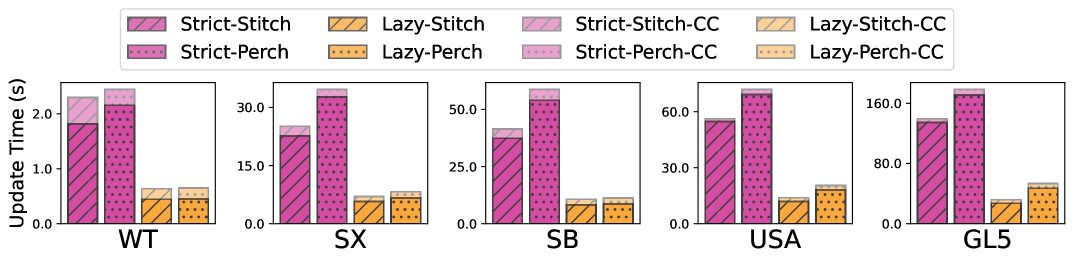
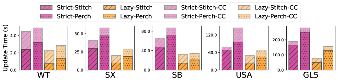
Figure 7: Overhead of maintaining the ordered set for offline queries.

Figure 8: Overhead of maintaining the ordered set for historical queries.

References

- [1]
- Acar et al. [2020] Umut A. Acar, Daniel Anderson, Guy E. Blelloch, Laxman Dhulipala, and Sam Westrick. 2020. Parallel Batch-Dynamic Trees via Change Propagation. In European Symposium on Algorithms (ESA). 2:1–2:23.
- Acar et al. [2005] Umut A Acar, Guy E Blelloch, and Jorge L Vittes. 2005. An experimental analysis of change propagation in dynamic trees. (2005).
- Ahn et al. [2012] Kook Jin Ahn, Sudipto Guha, and Andrew McGregor. 2012. Analyzing graph structure via linear measurements. In ACM-SIAM Symposium on Discrete Algorithms (SODA). SIAM, 459–467.
- Anderson et al. [2020] Daniel Anderson, Guy E. Blelloch, and Kanat Tangwongsan. 2020. Work-Efficient Batch-Incremental Minimum Spanning Trees with Applications to the Sliding-Window Model. In ACM Symposium on Parallelism in Algorithms and Architectures (SPAA).
- Bearman et al. [2004] Peter S Bearman, James Moody, and Katherine Stovel. 2004. Chains of affection: The structure of adolescent romantic and sexual networks. American journal of sociology 110, 1 (2004), 44–91.
- Bisenius et al. [2018] Patrick Bisenius, Elisabetta Bergamin, Eugenio Angriman, and Henning Meyerhenke. 2018. Computing top-k closeness centrality in fully-dynamic graphs. In 2018 Proceedings of the Twentieth Workshop on Algorithm Engineering and Experiments (ALENEX). SIAM, 21–35.
- Boruvka [1926] Otakar Boruvka. 1926. O jistém problému minimálním. Práce Mor. Prırodved. Spol. v Brne (Acta Societ. Scienc. Natur. Moravicae) 3, 3 (1926), 37–58.
- Chazelle et al. [2005] Bernard Chazelle, Ronitt Rubinfeld, and Luca Trevisan. 2005. Approximating the Minimum Spanning Tree Weight in Sublinear Time. SIAM J. on Computing 34, 6 (2005).
- Chen et al. [2022] Qing Chen, Sven Helmer, Oded Lachish, and Michael Bohlen. 2022. Dynamic spanning trees for connectivity queries on fully-dynamic undirected graphs. Proceedings of the VLDB Endowment 15, 11 (2022), 3263–3276.
- Ciaperoni et al. [2020] Martino Ciaperoni, Edoardo Galimberti, Francesco Bonchi, Ciro Cattuto, Francesco Gullo, and Alain Barrat. 2020. Relevance of temporal cores for epidemic spread in temporal networks. Scientific reports 10, 1 (2020), 12529.
- Crouch et al. [2013] Michael S Crouch, Andrew McGregor, and Daniel Stubbs. 2013. Dynamic graphs in the sliding-window model. In European Symposium on Algorithms (ESA). Springer, 337–348.
- da Trindade et al. [2024] Joana MF da Trindade, Julian Shun, Samuel Madden, and Nesime Tatbul. 2024. Kairos: Efficient Temporal Graph Analytics on a Single Machine. arXiv preprint arXiv:2401.02563 (2024).
- Dhouib [2024] Souhail Dhouib. 2024. Innovative method to solve the minimum spanning tree problem: The Dhouib-Matrix-MSTP (DM-MSTP). Results in Control and Optimization 14 (2024), 100359.
- Ding et al. [2025] Xiangyun Ding, Yan Gu, and Yihan Sun. 2025. Source Code. https://github.com/ucrparlay/AM-tree.
- Driscoll et al. [1989] James R. Driscoll, Neil Sarnak, Daniel D. Sleator, and Robert E. Tarjan. 1989. Making data structures persistent. J. Computer and System Sciences 38, 1 (1989), 86–124.
- Eppstein [1994] David Eppstein. 1994. Offline algorithms for dynamic minimum spanning tree problems. Journal of Algorithms 17, 2 (1994), 237–250.
- Ferragina and Luccio [1996] Paolo Ferragina and Fabrizio Luccio. 1996. Three techniques for parallel maintenance of a minimum spanning tree under batch of updates. Parallel Processing Letters 6, 02 (1996), 213–222.
- Gandhi and Simmhan [2020] Swapnil Gandhi and Yogesh Simmhan. 2020. An interval-centric model for distributed computing over temporal graphs. In International Conference on Data Engineering (ICDE). IEEE, 1129–1140.
- Hanauer et al. [2021] Kathrin Hanauer, Monika Henzinger, and Christian Schulz. 2021. Recent advances in fully dynamic graph algorithms. arXiv preprint arXiv:2102.11169 (2021).
- Henzinger et al. [2020] Monika Henzinger, Stefan Neumann, and Andreas Wiese. 2020. Dynamic Approximate Maximum Independent Set of Intervals, Hypercubes and Hyperrectangles. In 36th International Symposium on Computational Geometry (SoCG 2020). Schloss Dagstuhl-Leibniz-Zentrum für Informatik.
- Holm et al. [2001] Jacob Holm, Kristian De Lichtenberg, and Mikkel Thorup. 2001. Poly-logarithmic deterministic fully-dynamic algorithms for connectivity, minimum spanning tree, 2-edge, and biconnectivity. J. ACM 48, 4 (2001), 723–760.
- Holm et al. [2015] Jacob Holm, Eva Rotenberg, and Christian Wulff-Nilsen. 2015. Faster fully-dynamic minimum spanning forest. In European Symposium on Algorithms (ESA). Springer, 742–753.
- Holme [2013] Petter Holme. 2013. Epidemiologically optimal static networks from temporal network data. PLoS computational biology 9, 7 (2013), e1003142.
- Holme and Saramäki [2012] Petter Holme and Jari Saramäki. 2012. Temporal networks. Physics reports 519, 3 (2012), 97–125.
- Huber et al. [2022] Andreas Huber, Daniel Thilo Schroeder, Konstantin Pogorelov, Carsten Griwodz, and Johannes Langguth. 2022. A streaming system for large-scale temporal graph mining of reddit data. In 2022 IEEE International Parallel and Distributed Processing Symposium Workshops (IPDPSW). IEEE, 1153–1162.
- Jarník [1930] Vojtěch Jarník. 1930. O jistém problému minimálním. Práca Moravské Prírodovedecké Spolecnosti 6 (1930), 57–63.
- Jayaram et al. [2024] Rajesh Jayaram, Vahab Mirrokni, Shyam Narayanan, and Peilin Zhong. 2024. Massively parallel algorithms for high-dimensional euclidean minimum spanning tree. In Proceedings of the 2024 Annual ACM-SIAM Symposium on Discrete Algorithms (SODA). SIAM, 3960–3996.
- Karger et al. [1995] David R Karger, Philip N Klein, and Robert E Tarjan. 1995. A randomized linear-time algorithm to find minimum spanning trees. J. ACM 42, 2 (1995), 321–328.
- Khan et al. [2012] Maleq Khan, VS Kumar, Gopal Pandurangan, and Guanhong Pei. 2012. A fast distributed approximation algorithm for minimum spanning trees in the SINR model. arXiv preprint arXiv:1206.1113 (2012).
- Kruskal [1956] Joseph B Kruskal. 1956. On the shortest spanning subtree of a graph and the traveling salesman problem. Proceedings of the American Mathematical society 7, 1 (1956), 48–50.
- Kwak et al. [2010] Haewoon Kwak, Changhyun Lee, Hosung Park, and Sue Moon. 2010. What is Twitter, a social network or a news media?. In International World Wide Web Conference (WWW). 591–600.
- Leskovec and Krevl [2014] Jure Leskovec and Andrej Krevl. 2014. SNAP Datasets: Stanford Large Network Dataset Collection. http://snap.stanford.edu/data.
- Li et al. [2018] Rong-Hua Li, Jiao Su, Lu Qin, Jeffrey Xu Yu, and Qiangqiang Dai. 2018. Persistent community search in temporal networks. In International Conference on Data Engineering (ICDE). IEEE, 797–808.
- Liu et al. [2022] Quanquan C Liu, Jessica Shi, Shangdi Yu, Laxman Dhulipala, and Julian Shun. 2022. Parallel Batch-Dynamic Algorithms for k-Core Decomposition and Related Graph Problems. In ACM Symposium on Parallelism in Algorithms and Architectures (SPAA). 191–204.
- McColl et al. [2013] Robert McColl, Oded Green, and David A Bader. 2013. A new parallel algorithm for connected components in dynamic graphs. In IEEE International Conference on High Performance Computing (HiPC).
- Meusel et al. [2014] Robert Meusel, Oliver Lehmberg, Christian Bizer, and Sebastiano Vigna. 2014. Web Data Commons — Hyperlink Graphs. http://webdatacommons.org/hyperlinkgraph.
- OpenStreetMap contributors [2010] OpenStreetMap contributors. 2010. OpenStreetMap. https://www.openstreetmap.org/.
- Pandey et al. [2021] Prashant Pandey, Brian Wheatman, Helen Xu, and Aydin Buluc. 2021. Terrace: A hierarchical graph container for skewed dynamic graphs. In IEEE International Conference on Data Mining (ICDM). 1372–1385.
- Pawagi and Kaser [1993] Shaunak Pawagi and Owen Kaser. 1993. Optimal parallel algorithms for multiple updates of minimum spanning trees. Algorithmica 9 (1993), 357–381.
- Peng et al. [2019] Richard Peng, Bryce Sandlund, and Daniel D Sleator. 2019. Optimal offline dynamic 2, 3-edge/vertex connectivity. In Algorithms and Data Structures: 16th International Symposium, WADS 2019, Edmonton, AB, Canada, August 5–7, 2019, Proceedings 16. Springer, 553–565.
- Prim [1957] Robert Clay Prim. 1957. Shortest connection networks and some generalizations. The Bell System Technical Journal 36, 6 (1957), 1389–1401.
- Reed [1978] David Patrick Reed. 1978. Naming and Synchornization in a Decentralized Computer System. (1978).
- Rocha and Blondel [2013] Luis EC Rocha and Vincent D Blondel. 2013. Bursts of vertex activation and epidemics in evolving networks. PLoS computational biology 9, 3 (2013), e1002974.
- Rossi and Ahmed [2015] Ryan A. Rossi and Nesreen K. Ahmed. 2015. The Network Data Repository with Interactive Graph Analytics and Visualization. In AAAI Conference on Artificial Intelligence. https://networkrepository.com
- Shen and Liang [1993] Xiaojun Shen and Weifa Liang. 1993. A parallel algorithm for multiple edge updates of minimum spanning trees. In International Parallel Processing Symposium (IPPS). IEEE, 310–317.
- Sleator and Tarjan [1983] Daniel D Sleator and Robert Endre Tarjan. 1983. A data structure for dynamic trees. J. Computer and System Sciences 26, 3 (1983), 362–391.
- Song et al. [2024] Jingyi Song, Dong Wen, Lantian Xu, Lu Qin, Wenjie Zhang, and Xuemin Lin. 2024. On Querying Historical Connectivity in Temporal Graphs. Proceedings of the ACM on Management of Data 2, 3 (2024), 1–25.
- Straka [2009] Milan Straka. 2009. Optimal worst-case fully persistent arrays. Trends in Functional Programming (2009).
- Sun et al. [2018] Yihan Sun, Daniel Ferizovic, and Guy E Blelloch. 2018. PAM: Parallel Augmented Maps. In ACM Symposium on Principles and Practice of Parallel Programming (PPOPP).
- Tarjan [1983] Robert Endre Tarjan. 1983. Data Structures and Network Algorithms. Society for Industrial and Applied Mathematics, Philadelphia, PA, USA.
- Tarjan and Werneck [2005] Robert Endre Tarjan and Renato Fonseca F Werneck. 2005. Self-adjusting top trees.. In SODA, Vol. 5. Citeseer, 813–822.
- Tench et al. [2024] David Tench, Evan West, Victor Zhang, Michael A Bender, Abiyaz Chowdhury, Daniel Delayo, J Ahmed Dellas, Martín Farach-Colton, Tyler Seip, and Kenny Zhang. 2024. GraphZeppelin: How to Find Connected Components (Even When Graphs Are Dense, Dynamic, and Massive). ACM Transactions on Database Systems 49, 3 (2024), 1–31.
- Tian et al. [2024] Anxin Tian, Alexander Zhou, Yue Wang, Xun Jian, and Lei Chen. 2024. Efficient Index for Temporal Core Queries over Bipartite Graphs. Proceedings of the VLDB Endowment 17, 11 (2024), 2813–2825.
- van Emde Boas [1977] Peter van Emde Boas. 1977. Preserving order in a forest in less than logarithmic time and linear space. Inform. Process. Lett. 6, 3 (1977), 80–82.
- Wang et al. [2021] Yiqiu Wang, Shangdi Yu, Laxman Dhulipala, Yan Gu, and Julian Shun. 2021. GeoGraph: A Framework for Graph Processing on Geometric Data. ACM SIGOPS Operating Systems Review 55, 1 (2021), 38–46.
- Xie et al. [2023] Haoxuan Xie, Yixiang Fang, Yuyang Xia, Wensheng Luo, and Chenhao Ma. 2023. On querying connected components in large temporal graphs. Proceedings of the ACM on Management of Data 1, 2 (2023), 1–27.
- Yang et al. [2023] Junyong Yang, Ming Zhong, Yuanyuan Zhu, Tieyun Qian, Mengchi Liu, and Jeffrey Xu Yu. 2023. Scalable Time-Range k-Core Query on Temporal Graphs. Proceedings of the VLDB Endowment 16, 5 (2023), 1168–1180.
- Yang et al. [2024] Junyong Yang, Ming Zhong, Yuanyuan Zhu, Tieyun Qian, Mengchi Liu, and Jeffrey Xu Yu. 2024. Evolution Forest Index: Towards Optimal Temporal k-Core Component Search via Time-Topology Isomorphic Computation. Proceedings of the VLDB Endowment 17, 11 (2024), 2840–2853.
- Yu et al. [2021] Michael Yu, Dong Wen, Lu Qin, Ying Zhang, Wenjie Zhang, and Xuemin Lin. 2021. On querying historical k-cores. Proceedings of the VLDB Endowment (2021).
- Zhang et al. [2024] Chao Zhang, Angela Bonifati, and M Tamer Özsu. 2024. Incremental Sliding Window Connectivity over Streaming Graphs. Proceedings of the VLDB Endowment 17, 10 (2024), 2473–2486.
- Zheng et al. [2008] Yu Zheng, Like Liu, Longhao Wang, and Xing Xie. 2008. Learning transportation mode from raw gps data for geographic applications on the web. In International World Wide Web Conference (WWW). 247–256.