Low-cost Embedded Breathing Rate Determination Using 802.15.4z IR-UWB Hardware for Remote Healthcare

Anton Lambrecht    Stijn Luchie    Jaron Fontaine    Ben Van Herbruggen    Adnan Shahid and Eli De Poorter Received 1 April 2025; The research that led to these results has received funding by the DistriMuSe project (HORIZON-KDT-JU-2023-2-RIA) with Grant No 101139769, from the Belgian Defense through contract number 24DEFRA009 and from the FWO PESSO project with Grant No 3G018522.The associate editor coordinating the review of this article and approving it for publication was …The authors are affiliated with IDLab, Department of Information Technology, Ghent University-imec, iGent Tower, Technologiepark-Zwijnaarde 15, B-9052 Ghent, Belgium. (email: Anton.Lambrecht@Ugent.be)

Abstract

Respiratory diseases account for a significant portion of global mortality. Affordable and early detection is an effective way of addressing these ailments. To this end, a low-cost commercial off-the-shelf (COTS), IEEE 802.15.4z standard compliant impulse-radio ultra-wideband (IR-UWB) radar system is exploited to estimate human respiration rates. We propose a convolutional neural network (CNN) to predict breathing rates from ultra-wideband (UWB) channel impulse response (CIR) data, and compare its performance with other rule-based algorithms. The study uses a diverse dataset of 16 individuals, incorporating various real-life environments to evaluate system robustness. Results show that the CNN achieves a mean absolute error (MAE) of 1.73 breaths per minute (BPM) in unseen situations, significantly outperforming rule-based methods (3.40 BPM). By incorporating calibration data from other individuals in the unseen situations, the error is further reduced to 0.84 BPM. In addition, this work evaluates the feasibility of running the pipeline on a low-cost embedded device. Applying 8-bit quantization to both the weights and input/ouput tensors, reduces memory requirements by 67% and inference time by 64% with only a 3% increase in MAE. As a result, we show it is feasible to deploy the algorithm on an nRF52840 system-on-chip (SoC) requiring only 46 KB of memory and operating with an inference time of only 192 ms. Once deployed, the system can last up to 268 days without recharging using a 20 000 mAh battery pack. For breathing monitoring in bed, the sampling rate can be lowered, extending battery life to 313 days, making the solution highly efficient for real-world, low-cost deployments.

breathing rate determination, convolutional neural network (CNN), impulse-radio ultra-wideband (IR-UWB), remote healthcare

1 Introduction

According to the Eurostat institution, diseases of the respiratory system accounted for 6.1% of all deaths in the EU in the year 2021 [1]. This statistic highlights the significant impact of respiratory issues on public health. Therefore, early detection effectively addresses these ailments [2, 3]. Timely identification significantly enhances the prospects of a complete recovery or allows for more effective management of symptoms. Proper monitoring of specific vital signs can play a significant role in facilitating this early detection process [4]. A variety of devices already exist to monitor breathing rate (BR) reliably. One example is a nasal pressure transducer, which measures airflow through the nostrils to track inhalation and exhalation phases. Another is the respiratory effort belt, worn around the chest or abdomen to monitor chest wall movement. While effective and widely used, these devices require direct skin contact, making them unsuitable for patient scenarios like burn victims, where attaching sensors could cause further harm. Additionally, constant monitoring throughout the day using contact-based solutions is inconvenient for individuals. A remote monitoring system could overcome these challenges, enabling respiratory data collection without causing discomfort. Such a system could have significant applications, for example in elderly care, stress and alertness monitoring.

This study uses a non-invasive radar system to measure respiratory rates by emitting signals and capturing their reflections, which vary with chest movements. The system does not require on-body sensors and is installed in front of the person, making it ideal for scenarios where the person faces a known direction. Example use cases include in-car monitoring of drivers or passengers, monitoring patients lying in bed or persons facing a known direction such as when seated in a chair or sofa.

For non-invasive breathing monitoring, multiple radar technologies are available, including mmWave, FMCW radar or ultra-wideband (UWB) radar. In this study, UWB radio technology was chosen for its use of large bandwidth, allowing the transmission of very short radio pulses lasting nanoseconds [5]. These very short UWB pulses and their reflections can be timestamped with high accuracy, allowing the detection of small chest movements. These precise distance measurements of chest movements are crucial for detecting breathing signals. Compared to alternative radar technologies, UWB also requires lower power consumption, is more affordable and generates minimal interference with other radio signals. Moreover, UWB radios can also be used for other purposes, such as communication or localization, making it a suitable technology for multi-functional systems that provide integrated sensing, localization and communication. Analyzing data from the radar hardware involves selecting from various processing techniques. While most studies on BR determination rely on signal processing methods, data driven-based approaches have shown promising results, particularly in challenging conditions [6, 7].

The key contributions of this work are the following:

• A convolutional neural network (CNN)-based processing pipeline is proposed for breathing determination that shows significant accuracy improvement as compared to basic rule-based processing techniques.

• The accuracy of the solution is extensively evaluated in various conditions, including an analysis of the generalization performance to unseen people and unknown environments.

• The impact of model quantization on accuracy, memory consumption, execution time, and energy consumption is modeled and analyzed for embedded devices.

• An open source dataset is provided consisting of UWB breathing data and annotated ground truth measurements captured using a low-cost commercial off-the-shelf (COTS) impulse-radio ultra-wideband (IR-UWB) device.

The remainder of the paper is organized as follows. First, Section 2 provides an overview of the current state of the art. Next, Section 3 provides a mathematical model of the system. Section 4 describes how the dataset was captured. Section 5 describes the algorithms developed to extract BR from the channel impulse response (CIR) data. Section 6 analyses the obtained results. Afterwards, Section 7 describes how the solution can be optimized and deployed on embedded hardware and analyses the reduced footprint, inference time, and power consumption. Finally, Section 8 concludes the paper and describes future work.

2 Related work

					Low-cost		Real life considerations
	Year	Device	Bandwidth (GHz)	IEEE comp- liant	COTS	Embedded impl.	Distance	Rotation	Environ- ment	Posture	Multiple persons in dataset	Multi- person	Non static
[8]	2017	NVA6201	2.3	-	-	-	-	-	-	-	✓	-	✓
[9]	2019	PulsOn 440	4.3	-	-	-	✓	-	-	-	✓	-	-
[10]	2020	X4	NA	-	-	-	-	✓	-	-	✓	-	-
[11]	2022	X4	NA	-	-	-	✓	✓	-	-	-	-	-
[12]	2022	X4M03	1.4	-	-	-	✓	-	-	-	✓	-	-
[13]	2023	Proprietary	0.5	✓	-	-	-	-	-	-	✓	✓	-
[14]	2020	X4	1.5	-	-	-	✓	✓	✓	-	-	-	-
[6]	2023	NVA6100	NA	-	-	-	-	-	✓	✓	✓	-	-
[7]	2024	X4M03	1.4	-	-	-	✓	✓	-	-	✓	-	-
[15]	2024	X4M05	1.4	-	-	-	✓	-	✓	-	✓	-	✓
[16]	2024	X4M06	NA	-	-	-	✓	✓	-	✓	-	-	✓
[17]	2022	X4m200	1.4	-	-	-	✓	-	✓	-	✓	✓	-
[18]	2017	NVA6201	2.3	-	-	-	✓	✓	-	-	✓	-	✓
[19]	2023	X4M03	1.4	-	-	-	✓	✓	-	-	✓	✓	✓
[20]	2023	NCJ29D5	0.5	✓	✓	-	✓	-	-	-	✓	-	-
This paper		DW3000	0.5	✓	✓	✓	✓	✓	✓	✓	✓	-	-

Table 1: Overview of related work, categorized by hardware type and application context. This work is the first to provide a truly low-cost, IEEE 802.15.4z-compliant, off-the-shelf available solution that can run on embedded hardware while coping with a variety of real-life environments and conditions.

Table 1 provides an overview of related scientific papers. As seen in the table, most studies employ radar systems designed by Novelda or Pulson devices, which consistently use high bandwidths of 1.4GHz or higher. A higher bandwidth enhances the precision of the CIR s, aiding in capturing subtle breathing patterns. However, such systems require more powerful downstream processing, reducing the cost-effectiveness of the system. These high-bandwidth devices are also not compliant with the IEEE 802.15.4z standard, lacking standardized bandwidth and center frequency configurations. Additionally, they are significantly more expensive, costing at least 10 times more than commercial standard-compliant transceivers such as Qorvo’s DW3000, which is priced under €10. Finally, most of these Novelda and Pulson devices are no longer commercially available.

Furthermore, as discussed in Section 1, capturing breathing movements is challenging since individuals are not always stationary or aligned with radar devices. Validation on diverse real-life conditions is essential to claim robustness. Columns 7 through 13 of Table 1 summarize these considerations across the reviewed papers. The Distance and Rotation columns indicate whether various distances and rotation angles between the person and radar were tested. Environment, Posture, and Multiple Persons in dataset denote whether the system was deployed in multiple rooms, included different postures, and featured multiple individuals. Multi-person specifies whether the solution was tested with multiple individuals simultaneously in front of the radar. Finally, Non-static indicates whether the person was performing any movements during the measurements.

When considering the solutions that use IEEE 802.15.4z-compliant hardware, the following work is most relevant. Farsaei et al. [13] utilize a 500 MHz standard-compliant radar system, but their hardware is proprietary and inaccessible, disqualifying it as COTS. Only 2 real-life considerations are tested using a peak-finding algorithm. In general, validation on BR determination is limited, as only 2 CIR-windows are considered in their validation set. Numan et al. [20] stands out for using the NCJ29D5 radar from NXP. This is a COTS device costing less than €10. The paper only evaluates generalizability to new individuals and over multiple distances. This work focuses more on presence detection and classifying low, normal, and high BR s rather than predicting the exact respiratory rates. BR determination is done with a peak detection-based solution, and its validation is restricted to 9, 10-second CIR windows.

Most prior work utilizes algorithm-based breathing rate estimators. A notable exception is Zhou et al. [19], which addresses a comparable number of challenges compared to this paper but lacks evaluations in multiple environments or with subjects in different postures. However, it does excel in analyzing non-static scenarios and multi-person setups. To tackle these challenging situations, the paper proposes an Attention-Based CNN-long short-term memory (LSTM) network to filter out human motion, after which a rule-based approach is used to obtain the BR. The computational complexity and low-cost aspects are not discussed, as the Novelda hardware and a very complex neural network (NN) is used.

The work described in this paper stands out from all works in Table 1 by using COTS IEEE 802.15.4z-compliant hardware, validating the system with multiple real-life considerations in mind and also analyzing the processing requirements of the solution. Compared to prior work, this study is the first to focus on low-cost and embedded hardware compatibility aspects.

3 System model

This study employs a radar-based system with a transmitter emitting signals that reflect off objects or people in the room. These reflections will be influenced by respiratory movements of the person in front of the radar and are subsequently captured by the receiver. The varying distance between the radar and the chest of the target is then used to extract the breathing rate [21]. Equation 1 shows mathematically how this distance is modelled.

$$d(t)=d_{0}+m(t)=d_{0}+m_{b}sin(2\pi f_{b}t)$$ (1)

where $f_{b}$ and $m_{b}$ are the breathing frequency and amplitude, respectively. The $d_{0}$ term represents the distance from the target to the radar. This paper only considers static targets, so in our work this term can be considered a constant. To extract respiratory information, UWB radio pulse signals are transmitted by a transmitter at regular intervals with a time interval in the order of milliseconds. These transmissions are also called slow-time samples. For each slow-time transmission, multiple reflections are received by a receiver, which are sampled as complex in-phase and quadrature (IQ) values with a resolution in the order of nanoseconds. Because of this higher sampling rate, these are also called fast-time samples. A collection of fast-time samples that correspond to 1 slow-time index forms a CIR. A collection of slow-time indices can then be represented as a matrix with the notation shown in Equation 2.

$$R={r[m,n]},1\leq m\leq N_{s},1\leq n\leq N_{f}$$ (2)

where each row corresponds to a CIR, $N_{s}$ is the number of slow-time samples and $N_{f}$ is the number of fast-time samples per CIR. Another way to interpret these indices is to consider the slow-time axis as discrete time instants and the fast-time indices as distances from the radar to the reflecting surfaces. Each transmitted signal represents a time step. Within this step, captured fast-time samples correspond to reflections originating from increasingly further distances. Consequently, taking more fast-time samples at a single slow-time index provides reflection data from more distant surfaces. Reflections originate not only from the target but also from static objects in the room. Assuming these objects are static, the received signal can be expressed as Equation 3.

$$r(t,\tau)=\sum_{i=0}A_{i}p(\tau-\tau_{i})+Ap(\tau-\tau_{d(t)})$$ (3)

where $t$ and $\tau$ are slow- and fast-times indices, respectively. The first term sums the static background reflections ($A_{i}$), also called clutter. The second term represents reflections from the target ($A_{p}$), where the time-dependent delay $\tau_{d}(t)$ varies with breathing. Fig. 2a illustrates the amplitude of a single CIR. The first path (FP) corresponds to where the amplitude of the captured IQ values rises above the noise floor. In Fig. 2a, this occurs at index 0.

4 Measurement campaign and dataset description

For evaluating the different algorithms, data was collected using the Qorvo DW3000, specifically the QM33120WDK1 development kit (DK), acting as a representative low-cost, COTS hardware device. The setup includes separate transmitter and receiver devices, each equipped with a Nordic nRF52840 DK and a DW3000 transceiver shield. The transmitter uses an omnidirectional antenna, while the receiver employs a directional antenna to focus on reflections coming from the desired direction. The system operates at a center frequency of 6.489 GHz with a bandwidth of 500 MHz. The slow-time sampling frequency is 77.5 Hz, and the receiver captures IQ samples at 1 ns intervals. Each fast-time sample represents 30 cm in distance, with each CIR containing 41 fast-time samples and the first peak always aligned at index 3. Samples before the first peak can be considered noise. The maximum distance the system can reach is equal to: $((41-4)*30~cm)/2=555~cm$. A Plux respiratory effort belt [22] serves as ground truth, measuring the accurate BR through belt stretch.

The dataset was collected in the Homelab in Zwijnaarde [23], a simulated home environment developed by Ghent University and imec for testing Internet of Things (IoT), smart home, and healthcare applications. The lab features various residential rooms, enabling diverse testing conditions. Fig. 1 illustrates the environments used in this project. To avoid saturation at the receiver side, the transmitter and receiver were placed 30 cm apart. In the first environment, targets lay in bed with the UWB hardware positioned 100 cm above their chest. In environments 2 and 3, participants sat on a chair at distances of 120 cm and 180 cm from the radar. Environment 4 involved standing individuals at varying distances (60, 100, 150, 200, and 400 cm) from the radar, with additional measurements at a 45-degree rotation angle for distances 60 cm and 150 cm. In the final environment, participants stood at the same distances without angle variations. For environments 4 and 5, both the transmitter and receiver were placed at a height of 156 cm. In total, 16 different people participated in the data campaign, resulting in a total of 240 different person-setup pairs. In environments 1, 2 and 3, measurements of 2 minutes were taken from each person-setup pair. In environments 4 and 5, only 1 minute CIR windows were captured. Consequently, approximately 288 min of data was obtained. To ensure variability in BR s, subjects followed a randomized breathing pattern guided by an app, producing rates between 6 and 20 breaths per minute (BPM).

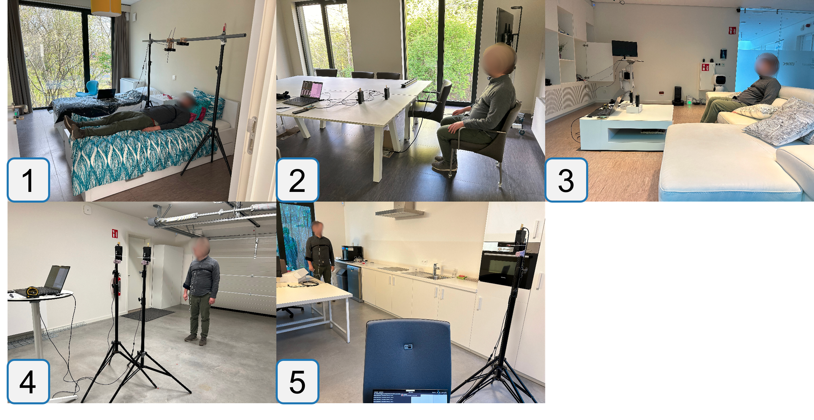
Figure 1: Samples were collected across various environments with 16 participants. Environment 1 had subjects lying down. Environments 2 and 3 had them sitting. In the final 2 environments, subjects stood at multiple distances and angles from the radar. Defining a setup as a distinct combination of environment, distance, angle, and posture resulted in 15 different setups.

5 Methodology

This section outlines the proposed processing pipeline, beginning with preprocessing steps and followed by different prediction algorithms. The prediction approaches are categorized into 2 types: rule-based peak-finding methods that serve as reference and the proposed model-based machine learning method.

5.1 Preprocessing

The preprocessing pipeline is shown in Figs. 2a to 2e. This pipeline processes the samples captured as IQ samples. For each slow-time sample, 41 fast-time samples are taken, forming a single CIR. Once collected, the amplitude of these samples is calculated. The resulting amplitude versus fast-time is shown in Fig. 2a. While phase information is also available, it is discarded due to unsynchronized transmitter and receiver clocks. These CIR s are then combined into a matrix, of which a heatmap representation is shown in Fig. 2b. Each row in the matrix corresponds to a CIR (the “slow time”’), and each column captures variations across time at a certain distance (the “fast time”). The maximum value of the slow-time index of the matrix is 120 seconds, representing all CIR samples collected from a single person in a specific environment and setup. To calculate the breathing rate over a shorter duration than the full experiment, a 30-second windowing operation is applied to the CIR matrix with a stride of 15 seconds. This window size was empirically determined to be an optimal balance between the dataset size required for model training and the accuracy of the fast fourier transform (FFT) that will be applied later in the pipeline. Using an overlapping windowing approach results in more training samples, which is advantageous for training a NN. Careful splitting between train and validation samples in our validation strategy will ensure no data leakage is introduced, which is further detailed in Section 6. An example of a window is shown in Fig. 2c. In this representation, it is clear that a periodic signal is present around range bin 8. In the next step, an FFT is applied to each column, generating a frequency spectrum for each distance bin. The obtained representation is shown on Fig. 2d, which is referred to as a range-frequency map. Peaks at the target breathing frequency are expected at the range index where a person is present. To focus on breathing rate-specific frequencies, signals below 0.09 Hz or above 0.5 Hz should be filtered out. When zooming in to this frequency range, peaks are indeed present in the example. Since the first peak index is present at index 3, the first 4 range bins can also be removed. Both the frequency filtering and range bin removal can be implemented with an image crop operation. The result of this operation is shown in Fig. 2e, showing which movement frequencies are present at each distance. The final step involves applying Min-Max normalization to scale all values between 0 and 1. This ensures consistent data scales across all CIR windows, which will benefit NN approaches. The min and max values are derived solely from the training data to prevent data leakage. The normalized CIR window then serves as input to the breathing detection algorithms, which in our case will be either peak finding techniques or neural networks.

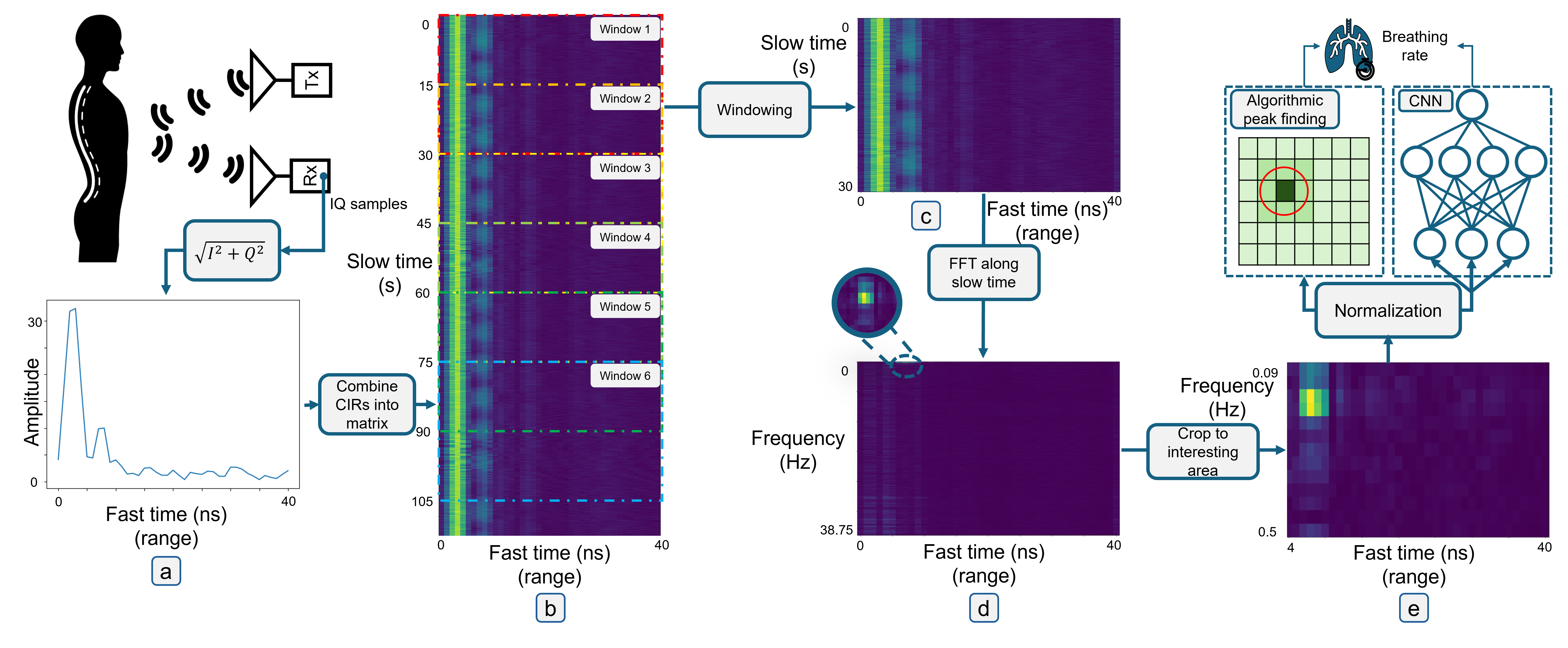
Figure 2: Visualization of processing pipeline. IQ samples coming from the receiver will serve as input for the pipeline. Each sub-representation of the data is described in Section 5 and is indicated with a letter at the bottom of the subfigure.

5.2 Peak finding techniques

As noted in Section 2, the most relevant low-cost or IEEE 802.15.4z-compliant studies are the papers by Numan et al. [20] and Farsaei et al. [13], both of which use rule-based approaches. To enable comparison, this first category of prediction methods includes 3 different rule-based frequency peak-finding techniques. The first one closely resembles the approach by Farsaei et al., from which the others are 2 variations. All algorithms use the range-frequency maps as input, which can be mathematically represented as: $M={m_{ij}},0<i<n;0<j<p$. Here, $m_{ij}$ is an element in the matrix, where $i$ represents the row index (frequency bin) and $j$ the column index (range bin). $n$ is the total number of frequency bins and $p$ is the number of fast-time indices. $f_{i}$ will be defined as the frequency associated with row $i$.

(i) The first approach identifies the breathing frequency by locating the row index $i_{max}$ of the maximum value in the matrix. Mathematically, this can be described as Equation 4. Once $i_{max}$ is found, the corresponding frequency bin is: $f_{pred}=f_{i_{max}}$. From now on, this method is called the highest peak algorithm.

$$i_{max}=arg\max_{i}(\max_{j}\{m_{ij}\})$$ (4)

(ii) In the second method, the distance-frequency map is first accumulated in 1 row with the operation described in Equation 5. After this, the highest frequency index can be determined with: $i_{max}=arg\max_{i}(a_{i})$. This solution is the accumulated highest peak algorithm. The rationale is that scattering causes signals influenced by breathing movements to propagate to more distant surfaces. When these reflections are captured, the frequency component of the breathing signal is also present at these distances. By accumulating, it is hypothesized that the breathing frequency will become more pronounced.

$$a_{i}=\sum_{j=1}^{p}m_{ij},j=1,2,...,p$$ (5)

(iii) The last algorithm employs the same accumulated row resulting from Equation 5. This time, the predicted frequency is determined by the weighted average operation described in Equation 6. Consequently, this solution is called the accumulated weighted average algorithm. Weighted averaging is also tested since this could alleviate the influence of large noise components.

$$f_{pred}=\sum_{i=1}^{n}\frac{a_{i}}{\sum_{i=1}^{n}{a_{i}}}f_{i}$$ (6)

5.3 Convolutional neural network based machine learning

The final method evaluated is a CNN. Among existing studies, only Zhou et al. [19] proposes an attention-based CNN-LSTM solution evaluated on a similar amount of real-world considerations as our dataset. A more simple CNN was chosen in this paper due to its significantly lower processing requirements, aligning better with the low-cost aspect of this paper. The model architecture and optimized parameters are detailed in Table 2. Various configurations of parameter sizes, kernel shapes, and layer counts were tested, with the best-performing design summarized in the table. A grid search was used to optimize normalization and regularization techniques, including batch normalization, dropout, and kernel regularization. The best-performing settings are also provided in Table 2. To ensure the robustness of the results, each model was trained 10 times over. The model that scored the median validation loss was selected. All subsequent reported results follow this training strategy.

Layer	Parameters
CIR _window (input)	size = (36, 13, 1)
conv2d	#filters = 8, kernel size = (10, 10), activation = relu, padding = same, kernel regularizer = L2
max_pooling2d	kernel size = (2, 2), strides = (2, 2)
conv2d_1	#filters = 16, kernel size = (8, 8), activation = relu, padding = same, kernel regularizer = L2
max_pooling2d_1	kernel size = (2, 2), strides = (2, 2)
conv2d_2	#filters = 32, kernel size = (4, 4), activation = relu, padding = same, kernel regularizer = L2
max_pooling2d_2	kernel size = (2, 2), strides = (2, 1)
conv2d_3	#filters = 64, kernel size = (2, 2), activation = relu, padding = same, kernel regularizer = L2
max_pooling2d_3	kernel size = (2, 2), strides = (2, 1)
dense	dim = 64, activation = relu, kernel regularizer = L2
dropout	drop out = 0.2
dense_1	dim = 16, activation = relu, kernel regularizer = L2
dropout_1	drop out = 0.2
dense_2 (output)	dim = 1

Table 2: Architecture of the proposed CNN for breathing rate prediction.

6 Results and analysis

This section evaluates the proposed CNN and compares it to the representative rule-based solutions. This is done by applying the algorithms to the dataset described in Section 4, comprising samples from 16 participants across 15 setups. Each of these participant-setup combinations forms a unique pair. For evaluating the generalizability of the solutions, specific pairs are excluded from the training data and used as validation samples. As a pair is always fully included or excluded from the training set, no data leakage will occur.

Three validation strategies are used to evaluate the generalizability of the model architecture. The leave-one-person-out cross-validation experiment assesses how well the proposed CNN handles unseen individuals. The leave-one-situation-out cross-validation experiment evaluates its ability to adapt to new setups. Finally, the leave-one-person-situation-pair-out cross-validation strategy examines how the system performs with new combinations of individuals and setups. These strategies can also be interpreted as follows. If the system, trained on a certain set of person-situation pairs, is deployed to track an entirely new person, the leave-one-person-out strategy will estimate its performance. For deployment in a previously unseen setup, the leave-one-situation-out analysis indicates the expected performance. In the leave-one-person-situation-pair-out strategy, the scenario involves introducing a new setup, where measurements for some participants already in the dataset are used as calibration data. The prediction is that the calibration data will enhance the model’s performance in the new setup.

6.1 Generalization to new persons

The first analysis evaluates the leave-one-person-out cross-validation strategy. In this approach, 1 participant is excluded from the training set in each fold and used for validation. This process is repeated for all 16 participants, producing 1 model per participant. The results are summarized in Table 3, showing the mean L1 errors and their standard deviation. For the highest peak method, mean L1 errors range from 3.10 BPM to 5.58 BPM. The accumulated distance-frequency map approach reduces mean L1 errors slightly, ranging from 2.75 BPM to 5.32 BPM. The weighted average algorithm shows L1 errors from 3.29 BPM to 4.46 BPM. Among the rule-based methods, selecting the highest peak from the accumulated frequency bins proves most effective. The table also includes results for our CNN model, where mean L1 errors range from 0.97 BPM to 2.51 BPM. This demonstrates a significant improvement compared to the rule-based solutions. Fig. 3 illustrates in which conditions the CNN outperforms traditional rule-based approaches. Fig. 3a shows a range-frequency representation in ‘simple’ conditions, where minimal noise was present. Hence, the breathing frequency peak is clearly visible and can be identified by most algorithms. However, in more challenging scenarios, where the noise becomes more pronounced, some noise frequency components may exceed the breathing signal. One example is shown in Fig. 3b. In these cases, the CNN performs better by not only analyzing the highest peak, but it can also take the higher harmonic components into account.

When compared to prior work, Farsaei et al. [13] and Numan et al. [20] report mean L1 errors of $<$1 BPM and 1.22$\pm$0.63 BPM, respectively. In comparison, the rule-based approaches evaluated here show worse L1 scores. Our CNN comes closer to this error but still results in a higher L1 error. This difference can be attributed to the inclusion of significantly more challenging scenarios and greater variability in BR s in our study. A fairer comparison is with the results from Zhou et al. [19], who report a mean L1 error of 2.3$\pm$1.9 BPM across various challenging scenarios. Our proposed CNN outperforms their results, with all validation folds in Table 3 achieving lower mean L1 scores.

	Highest peak		Accumulated highest peak		Accumulated weighted average		CNN
Pers.	mean (BPM)	std (BPM)	mean (BPM)	std (BPM)	mean (BPM)	std (BPM)	mean (BPM)	std (BPM)
1	3.94	4.20	3.13	2.79	3.89	2.18	1.65	1.24
2	4.20	4.02	4.05	3.85	4.34	2.51	2.08	1.52
3	5.38	4.34	5.32	4.89	3.54	2.50	2.51	2.33
4	4.31	4.14	2.87	3.32	3.85	2.27	1.51	1.30
5	4.57	4.25	3.76	3.97	3.57	2.39	1.59	1.27
6	4.15	3.48	3.83	3.54	3.64	2.63	2.06	1.5
7	3.61	3.15	2.97	3.18	3.57	1.88	0.97	0.83
8	4.94	4.19	3.58	3.70	3.80	2.66	2.17	1.57
9	5.58	4.67	4.10	3.67	3.99	2.56	2.05	1.80
10	4.19	4.53	2.75	3.06	4.26	2.32	1.35	1.18
11	3.10	3.40	3.19	3.65	4.25	2.34	1.64	1.48
12	3.67	3.14	3.33	2.99	4.46	2.19	1.83	1.34
13	4.19	4.49	2.98	2.89	4.10	2.27	1.89	1.29
14	3.29	3.26	2.80	3.10	3.98	2.21	1.54	1.38
15	3.52	3.78	2.86	3.41	3.29	2.42	1.34	1.11
16	3.61	3.74	3.01	3.92	4.22	2.07	1.19	0.97

Table 3: Mean and standard deviation of the L1 error obtained when predicting the breathing rate of unseen persons. The CNN performs better than rule-based techniques, with mean accuracies between 0.97 and 2.51 BPM and lower standard deviations.

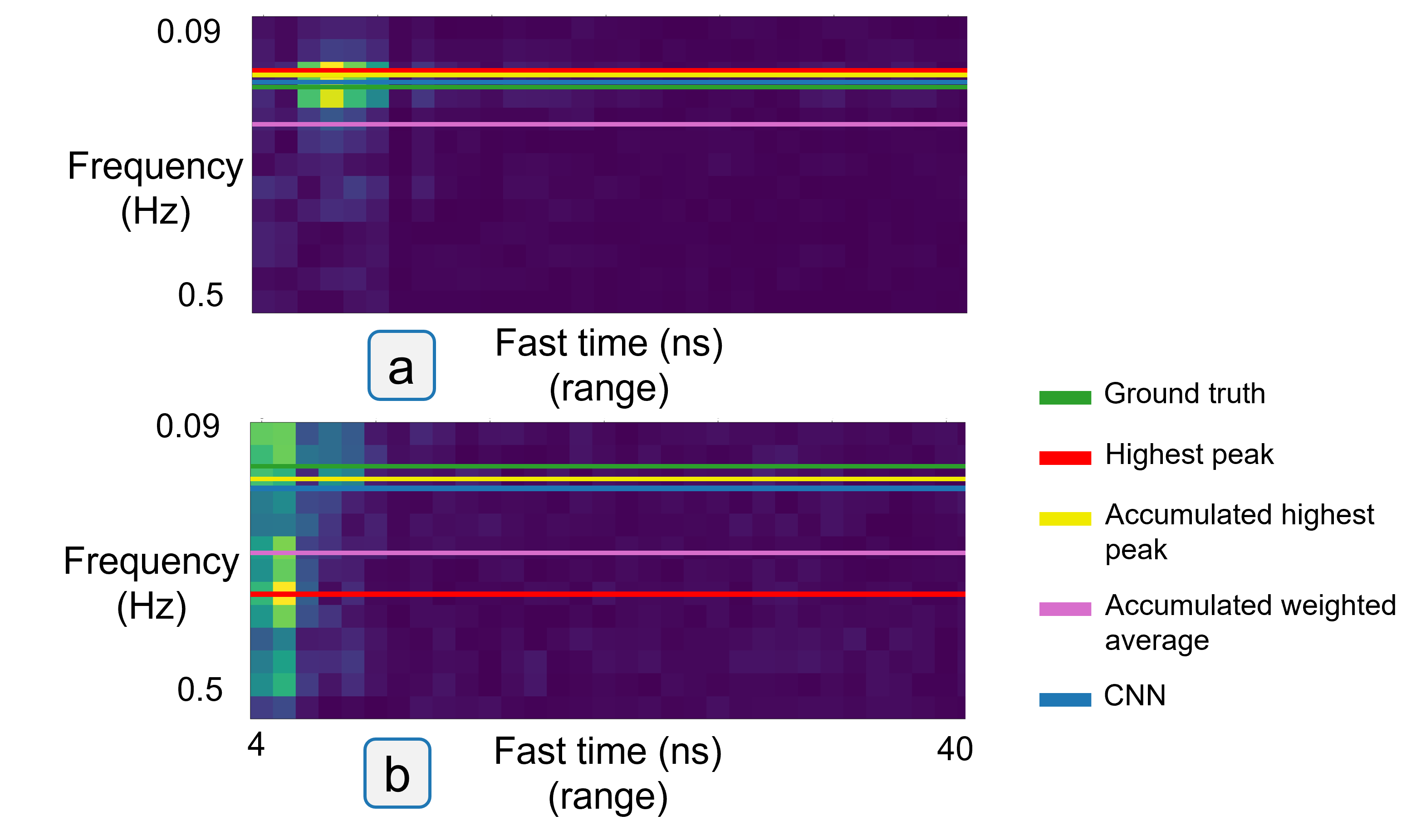
Figure 3: The breathing rate estimates of the rule-based algorithms and the proposed CNN are visualized on a range-frequency map. In a simple scenario with a visible peak, shown in (a), the predictions from all methods closely align. However, in noisier scenarios where the peak is less distinct, as shown in (b), the CNN predictions are significantly closer to the ground truth.

6.2 Generalization to new situations

The leave-one-setup-out cross-validation strategy evaluates generalizability to unseen setups. In each fold, 1 setup is entirely excluded for validation. Fig. 4 presents the results, where red box plots show the CNN performance, and the green, yellow, and purple plots represent the highest peak, accumulated highest peak, and accumulated weighted average algorithms. The box plots display L1 errors across validation samples, with the x-axis indicating the setup parameters in the validation set. The results confirm that the CNN generally outperforms rule-based methods. Only in setup 1 do the highest peak and accumulated highest peak algorithms slightly outperform the CNN. However, this difference is negligible.

Compared to prior work, the performance of the rule-based solutions are very close to the results reported in the papers from Farsaei et al. [13] and Numan et al. [20] for the “simple” situations 1 and 2. When considering more difficult situations, which are not considered in the works above, the algorithms start to fail, whereas the CNN still provides reasonable accuracies for these challenging, unseen conditions.

Finally, we consider a situation whereby a situation has been observed, but a new person is monitored for which the CNN was not trained. This “leave-one-person-setup-pair-out” cross-validation strategy assesses performance when data from a specific person-setup pair is excluded. The results are represented by the blue box plots in Fig. 4. These box plots show that when training includes data from other individuals in the same setup, the CNN significantly improves its performance in fully unseen setups. With this strategy, only setup 10 has a Q3 above 2 BPM, indicating robust performance in nearly all scenarios.

6.3 Influence of situation parameters

Based on the results in Fig. 4, several conclusions can be made concerning the influence of setup parameters on CNN performance. In this analysis, the results from the leave-one-person-setup-pair-out cross-validation are considered. First, the posture of the target person significantly impacts performance. Analyzing individuals lying down is the easiest due to minimal random body movement (RBM). Sitting down introduces additional challenges due to increased reflection angles and slightly higher RBM. Standing is the most difficult posture, consistently yielding poorer results at the same distances. The effect of distance is best represented in the scenarios where the individuals were standing. The accuracy generally decreases as the distance between the target and radar increases from 100 to 400 cm due to the decreased strength of the reflected signal. However, the CNN still provides an acceptable mean accuracy of 1.29 BPM at a 4-meter distance. Interestingly, there is a significant performance drop at a distance of 60 cm. This results from the fixed radar height of 156 cm (as noted in Section 4) for environments 4 and 5. This height exceeds typical chest level, causing signals to arrive at steeper angles for shorter individuals, especially at close range. Additionally, at 60 cm, target reflections may overlap with first peak signals from the transmitter. For use cases where shorter ranges are required, the transmitter and receiver can be set up closer together. This would alleviate first peak overlap for shorter ranges but would require the transmission power to be lower to limit the saturation of the receiver. Finally, regarding the body angle, the CNN provides an acceptable mean error of 0.86 BPM even when the target person is positioned at a 45-degree angle towards the radar. This demonstrates that the CNN can handle such scenarios effectively.

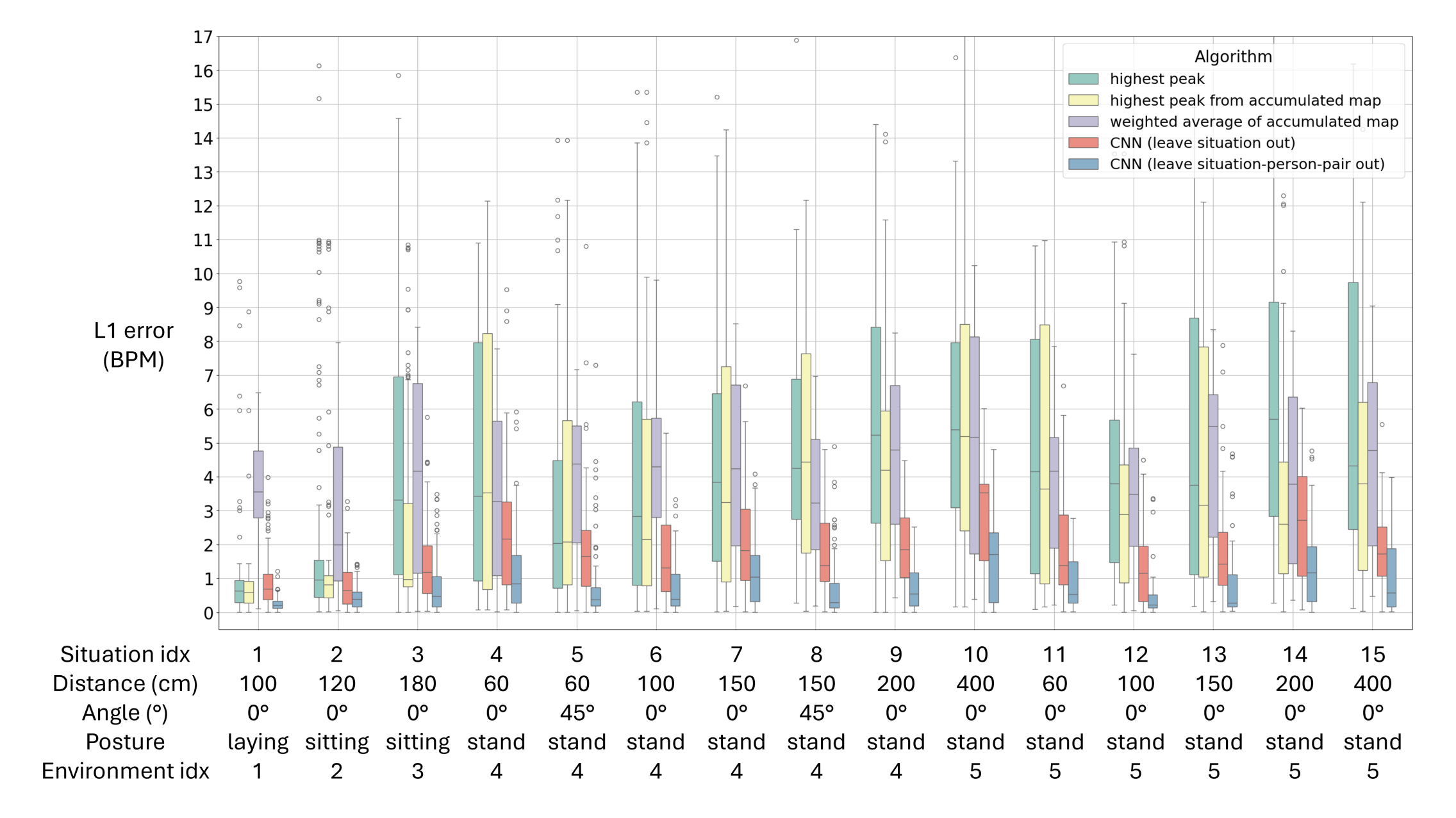
Figure 4: Breathing rate prediction errors in different situations (environment, posture, distance and body angle). The green, yellow and purple plots are the results when applying the rule-based methods described in Section 5.2. The red plots correspond to the L1 errors of the CNN for fully unseen situations. The blue box plots correspond to the L1 errors of the CNN for predicting the breathing rate for a new unseen person when other persons have already been observed in the specific situation (e.g. some form of pretraining on other individuals was possible). The CNN achieves a MAE of 1.73 BPM in unseen situations, significantly outperforming rule-based methods (3.40 BPM). When pretraining is possible, the MAE of the CNN is further reduced to 0.84 BPM.

7 Deploying on embedded hardware

Finally, this section thoroughly evaluates the feasibility of deploying the proposed solution on constrained hardware. First, the radar’s slow-time sampling frequency is analyzed. The second subsection will give an assessment of the preprocessing pipeline’s computational complexity. In the following section, the resource usage of the CNN-based solution is examined. The evaluation is conducted by deploying the model on the nRF52840 system-on-chip (SoC) to verify whether the model can run directly on the receiver device. In the final section, the power usage of the complete solution is described.

7.1 Required sampling rate

This section addresses the question of how often the UWB transmitter should transmit a packet. The maximum sampling rate of our system is empirically determined to be 77.5 Hz. A higher sampling frequency requires sending more packets, which is not desirable for battery-powered embedded solutions. The red curve in Fig. 5 illustrates the leave-one-setup-out cross-validation results on subsampled datasets. Limiting the sampling rate to 20 Hz has minimal impact on L1 error, but reducing it further significantly increases error. Given that human BR s peak at 0.5 Hz, Nyquist’s theorem requires a minimal sampling rate of 1.0 Hz. The blue curve, representing the errors obtained when only validating on situation 1, shows that lower sampling rates have less impact in less complex conditions, with performance declining only at 4 Hz.

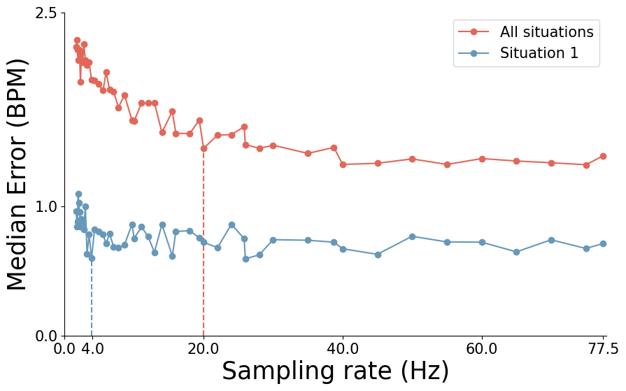
Figure 5: Median L1 error for different sampling rates. Lowering the sampling rate negatively affects L1 error. For easy situations (situation 1), the sampling rate can be lowered to 4 Hz. When also considering more difficult situations, sampling rate should remain above 20 Hz.

7.2 Algorithmic complexity of preprocessing pipeline

This section theoretically analyzes which parameters most profoundly impact the computation complexity of the preprocessing pipeline. First, the pipeline applies an FFT to each 30-second range bin. This FFT operation has a complexity of $O(n~\log~n)$, with $n$ the array length. Since an FFT is performed for each fast-time index, indicated by $m$, the total complexity becomes $O(mn\log~n)$. Next, a cropping operation reduces the window size from $(n,m)$ to $(k,r)$, where $k$ is the number of frequency bins and $r$ is the number of range bins after cropping. This slicing operation has a complexity of $O(kr)$. Finally, a normalization operation is applied by using an element-wise subtraction and division operation. Both these operations have a complexity of $O(k~r)$. All previous steps can be summarized as $O(mn~\log~n+3kr)$. Since $m$ and $r$ are radio configuration-dependent constants, this simplifies to $O(n\log~n+k)$. The dominant term, being $O(n\log~n)$, indicates an acceptable computational load suitable for constrained hardware.

7.3 Memory usage of the CNN model

One consideration with the CNN-based solution is its higher memory requirements compared to rule-based approaches. As the model size grows, the memory demand increases, limiting deployment on embedded devices. The proposed CNN architecture occupies 141 KB. This is already an acceptable model size as the nRF52840 SoC, with 256 KB static random access memory (SRAM) and 1 MB flash memory available, can run this model. Further memory reduction can be achieved through quantization. This technique lowers the precision of the model parameters, converting the standard 32-bit floating-point values to lower-bit formats. In this case, the model parameters will be converted to 8-bit unsigned integers. In addition to quantizing the model parameters, the input and output tensors are also quantized, resulting in the entire network operating in 8-bit integer format. After this operation, the model size is reduced by 67 % or to 46 KB, at the cost of only a 3.15 % increase in MAE due to the mismatch between the float32 to int8 transformation operation, making it suitable for severely memory-constrained devices.

7.4 Execution time of the system

Next, we experimentally measure the execution time of the different approaches. Using the rule-based techniques results in an inference time of 0.139 ms. The inference time of the CNN is higher at 538 ms. However, since 30-second windows are processed, the CNN’s inference time is still significantly shorter than the considered time window. Reducing the inference time is still beneficial for embedded devices because this leaves more processing time for other tasks and allows the hardware to enter energy-saving states sooner. Quantization, as described earlier, not only reduces memory usage but also lowers inference time. When deploying the quantized model on the nRF52840 SoC, the inference time is reduced to 192 ms, which is a 64% reduction. The nRF52840 SoC includes a floating-point unit (FPU), which helps handle floating-point operations. On microcontrollers without this support, the benefits of the quantized model would be even more pronounced.

7.5 Energy consumption

7.5.1 Experimental measurement of the energy consumption

This section examines the energy consumption of the solution. The practical energy consumption was determined by deploying all components of the processing pipeline on the nRF52840 DK platform and measuring the current draw with a Keysight N6705B DC Power Analyzer. As the hardware was powered with a USB cable, the supply voltage was set to 5 V. Note that the currents mentioned here are averages, while the reported energy consumptions are precise area-under-the-curve calculations. Total energy consumption per 30-second window can be calculated using Equation 7.

$$\begin{split}E_{30sec}=&\underbrace{E_{plat}+E_{TX}}_{TX}\\ &+\underbrace{E_{plat}+E_{RX}+E_{preproc}+E_{model}}_{RX}\end{split}$$ (7)

This formula includes the energy consumption of the platform ($E_{plat}$), transmitter ($E_{TX}$), receiver ($E_{RX}$), preprocessing pipeline ($E_{preproc}$), and CNN model ($E_{model}$). Since the transmitter and receiver are separate devices, the platform’s energy must be counted twice. As all CIR s are collected at the receiver, processing will occur at the receiver side. The nRF52840 DK platform consumes $1.84~mA$ on average at $5~V$, resulting in an energy consumption of $E_{plat}=0.277~J$ over 30 seconds.

As shown in Section 7.1, the system works well at a sampling rate of 20 Hz. In this case, transmitter and receiver consume $0.0447~J$ and $0.0637~J$ per second, respectively. Over 30 seconds, this totals to $E_{TX}=1.342~J$ and $E_{RX}=1.912~J$. Preprocessing occurs once every 30 seconds, consuming $2.01~mA$ over $0.110~s$, which equals $E_{preproc}=0.001~J$. The CNN analysis uses $4.56~mA$ over $0.523~s$, consuming $0.012~J$. Quantizing the model reduces current draw to $4.17~mA$ and inference time to $0.199~s$, reducing energy consumption to $E_{model}=0.004~J$. Total energy consumption over 30 seconds is $E_{30sec}=3.813~J$. In other words, the system consumes $0.127~W$ on average. With an AAA battery providing $5400~J$, 1 battery can power the system for approximately 11.8 hours. Since each battery provides only $1.5~V$, at least 4 batteries are needed to power the $5~V$ system. Section 7.1 also states that the sampling rate can be lowered to 4 Hz in more simple situations. This lowers power consumption of the transmitter and receiver to $0.0436~J$ and $0.0547~J$ per second, respectively. Over 30 seconds, this becomes $E_{TX}=1.307~J$ and $E_{RX}=1.640~J$. The preprocessing step was also tested at this lowered sampling rate, but no measurable differences were observed. Recalculating with these numbers, show that the system consumes $0.117~W$ at a sampling rate of 4 Hz. This corresponds to 12.8 hours of constant monitoring with 4 AAA batteries.

7.5.2 Theoretical energy consumption model

In the previous calculations, the degrees of freedom are limited by the development boards used. For practical deployments, energy consumption can be significantly reduced.

(i) A first optimization is to deploy the transmitter and receiver on 1 platform. By doing this, only 1 $E_{plat}$ term remains in the energy calculation. To this end, different antenna designs should minimize self-interference between the transmitting and receiving antenna [24].

(ii) Secondly, note that the transmitter and receiver make up 84 % of the total power consumption. Part of this can be attributed to the fact that a DK is used that is not fully optimized for energy consumption. Using the information stated in the datasheet of the DW3000 transceivers [25], a theoretical minimal current profile can be calculated for both the transmitter and receiver. The current consumption of the transceiver will vary in time depending on the state in which the transceiver is. Equation 8 shows the calculation of the theoretical minimal energy consumption when the transceiver is in transmitter mode. Equation 9 calculates the used energy for the receiver. In these formulas, $E_{PLL}$ represents the energy consumed by the phase locked loop (PLL) phase, $E_{TX\_SHR}$ and $E_{RX\_SHR}$ denote the energy used while transmitting and receiving the synchronization header (SHR), and $E_{TX\_PHR\_PSDU}$ and $E_{RX\_PHR\_PSDU}$ correspond to the energy consumed during the transmission and reception of the physical layer header (PHR) and physical layer service data unit (PSDU). Additionally, $E_{PR\_{HUNT}}$ is the energy used during the preamble hunt phase, which involves the receiver searching for and detecting the preamble signal to synchronize with the incoming data transmission. $E_{RC}$ is the energy consumed in the receiver chain during the IDLE_RC phase, and $E_{SLEEP}$ represents the energy used when the transceiver is in a low-power sleep state.

$$\begin{split}E_{TX\_min}=&E_{PLL}+E_{TX\_SHR}\\ &+E_{TX\_PHR\_PSDU}+E_{SLEEP}\end{split}$$ (8)

$$\begin{split}E_{RX\_min}=&E_{PLL}+E_{PR\_HUNT}\\ &+E_{RX\_SHR}+E_{RX\_PHR\_PSDU}\\ &+E_{PLL}+E_{RC}+E_{SLEEP}\end{split}$$ (9)

(iii) Thirdly, another major improvement can be made for the receivers’ $E_{PR\_HUNT}$ term. The DK receiver automatically reverts to the preamble hunt phase after receiving a packet. In the context of this solution, the timings between the transmitter and receiver are precisely defined. Also, as stated in optimization 1, both transmitter and receiver are deployed on a single platform, making it possible to share the same clock. This enables us to minimize this preamble hunt phase, leading to a negligible phase hunt duration.

(iv) A final optimization concerns IDLE current usage of the transceivers. The development kit hardware lacks deep sleep capability and instead defaults to the PLL state, which consumes significantly more power. By implementing this functionality in the deployment version of the system, power consumption will be significantly reduced.

State	State name	T (ms)	I (mA)	E (mJ)
Transmitter
1	PLL lock	0.020	18	0.00108
2	TX SHR	0.270	48	0.03888
3	TX PHR/PSDU	0.016	40	0.0019
4 (4Hz)	SLEEP	249.694	0.00026	0.00078
4 (20Hz)	SLEEP	49.694	0.00026	0.00078
Receiver
1	PLL lock	0.020	18	0.00108
2	PR_HUNT	0.000	70	0
3	RX SHR	0.24	78	0.05616
4	RX PHR/PSDU	0.016	70	0.00336
5	PLL lock	0.02	18	0.00108
6	IDLE RC	0.036	8	0.000864
7 (4 Hz)	SLEEP	249.668	0.00026	0.00078
7 (20 Hz)	SLEEP	49.668	0.00026	0.00078

Table 4: Theoretical duration and current usage of transmitter and receiver in the different states of the energy model.

Theoretical durations and current usages are presented in Table 4. Note that the transceiver operates at 3V, so all energy calculations were performed with this voltage in mind. The transmitter starts in the PLL state, using 18 mA for 0.020 ms. It then transmits the SHR, which is 256 symbols long, taking 0.270 ms and consuming 48 mA. Next, the PHR and PSDU are sent. For CIR collection, empty packets can be sent, but the PSDU will still contain the medium access control (MAC) header and reed solomon (RS) bits, taking 0.016 ms and consuming 40 mA. The transmitter then transitions into a deep sleep state for the rest of the 250 or 50-millisecond period, based on the configured sampling rate. In this case, 4 Hz and 20 Hz are shown. This state is very efficient, with a consumption of only 0.00026 mA. The receiver also starts in the PLL state and then skips the HUNT state. After this, the receiving device sequentially acquires the SHR, PHR, and PSDU, ending with another PLL, IDLE RC, and deep sleep state. When considering the system with a sampling rate of 20 Hz, 1 propagation sums to $0.0419~mJ$ for the transmitter and $0.0626~mJ$ for the receiver. This is executed 20 times per second over a period of 30 seconds, resulting in $E_{TX\_min}=0.025~J$ and $E_{RX\_min}=0.0375~J$. Substituting these theoretical minima in Equation 7, gives $E_{30\_sec\_min}=0.345~J$. Consequently, on average 0.0115 W is used, allowing the optimized system to run for 130.5 hours on four AAA batteries. A more realistic deployment option is a common battery pack of 20 000 mAh. This configuration could enable the system to work for 268.2 days without recharging. In less complex situations, where a sampling rate of 4 Hz is sufficient, $E_{TX\_min}$ and $E_{RX\_min}$ decrease to $0.005~J$ and $0.008~J$. Consequently, $E_{30\_sec\_min}$ becomes $0.295~J$, enabling continuous monitoring for approximately 313.8 days. This allows for BR monitoring in locations without power outlets, such as movable beds, furniture, and desks.

8 Conclusion

This research successfully developed and validated a non-intrusive system for accurate BR monitoring. The proposed solution has potential applications across diverse domains, including remote patient monitoring, stress detection in vehicles and ships, and presence detection in smart homes. A CNN model, trained and evaluated on a novel, open source dataset, demonstrated significantly superior performance compared to existing approaches. Robustness was extensively tested across challenging conditions. The system maintained accuracy at distances up to 4 meters, achieving an average L1 error of 2.41 BPM, which was further reduced to 1.29 BPM with calibration pretraining. Accurate results were also obtained with different body angles, showing a mean error of 0.86 BPM at 45 degrees. Moreover, the system demonstrated generalizability by accurately performing in unseen environments and with subjects in various postures. Deployment feasibility was shown using a low-cost, COTS radar setup and optimized processing, enabling operation on resource-constrained hardware. Practical analysis revealed 11.8 hours of continuous monitoring using 4 AAA batteries at a sampling rate of 20 Hz. Theoretical optimizations indicate the potential for significantly extended battery life, suggesting up to 130.5 hours of operation on AAA batteries, or 268.2 days with a common battery pack. For less complex situations, sampling rate can be lowered to 4 Hz. This decrease in sampling frequency extends the theoretical battery life to 313.8 days. Future research will address even more real-world complexities such as multi-person detection and non-static subjects and explore integration with communication modules for joint communication and sensing (JCAS) applications.

References

- [1] Eurostat. (2024) Respiratory diseases statistics. [Online]. Available: https://ec.europa.eu/eurostat/statistics-explained/index.php?title=Respiratory_diseases_statistics
- [2] J. Bousquet, C. Tanasescu, T. Camuzat, J. Anto, F. Blasi, A. Neou, S. Palkonen, N. Papadopoulos, J. Antunes, B. Samolinski, P. Yiallouros, and T. Zuberbier, “Impact of early diagnosis and control of chronic respiratory diseases on active and healthy ageing: A debate at the European Union Parliament,” Allergy, vol. 68, no. 5, pp. 555–561, May 2013.
- [3] K. Kostikas, D. Price, F. S. Gutzwiller, B. Jones, E. Loefroth, A. Clemens, R. Fogel, R. Jones, and H. Cao, “Clinical Impact and Healthcare Resource Utilization Associated with Early versus Late COPD Diagnosis in Patients from UK CPRD Database,” International Journal of Chronic Obstructive Pulmonary Disease, vol. 15, pp. 1729–1738, 2020.
- [4] S. A. Kayser, R. Williamson, G. Siefert, D. Roberts, and A. Murray, “Respiratory rate monitoring and early detection of deterioration practices,” British Journal of Nursing, vol. 32, no. 13, pp. 620–627, Jul. 2023.
- [5] M. Cheraghinia, A. Shahid, S. Luchie, G.-J. Gordebeke, O. Caytan, J. Fontaine, B. V. Herbruggen, S. Lemey, and E. D. Poorter, “A comprehensive overview on uwb radar: Applications, standards, signal processing techniques, datasets, radio chips, trends and future research directions,” IEEE Communications Surveys & Tutorials, pp. 1–1, 2024.
- [6] Q. Li, J. Liu, R. Gravina, W. Zang, Y. Li, and G. Fortino, “A uwb-radar-based adaptive method for in-home monitoring of elderly,” IEEE Internet of Things Journal, vol. 11, no. 4, pp. 6241–6252, 2024.
- [7] W. Mu, J. Zhang, X. Jiang, K. Wang, L. Li, and L. Zhang, “Ap-hr: Amplitude and phase joint optimization-based heartbeat and respiration separation algorithm using ir-uwb radar,” in 2024 IEEE International Workshop on Radio Frequency and Antenna Technologies (iWRF&AT), 2024, pp. 265–270.
- [8] S. K. Leem, F. Khan, and S. H. Cho, “Vital sign monitoring and mobile phone usage detection using ir-uwb radar for intended use in car crash prevention,” Sensors, vol. 17, no. 6, 2017.
- [9] Z. Duan and J. Liang, “Non-contact detection of vital signs using a uwb radar sensor,” IEEE Access, vol. 7, pp. 36 888–36 895, 2019.
- [10] Y. Zhang, X. Li, R. Qi, Z. Qi, and H. Zhu, “Harmonic multiple loop detection (hmld) algorithm for not-contact vital sign monitoring based on ultra-wideband (uwb) radar,” IEEE Access, vol. 8, pp. 38 786–38 793, 2020.
- [11] M. Husaini, L. M. Kamarudin, A. Zakaria, I. K. Kamarudin, and M. A. Ibrahim, “Non-contact vital sign monitoring during sleep through uwb radar,” in 2022 10th International Conference on Information and Communication Technology (ICoICT), 2022, pp. 157–162.
- [12] A. Lopes, D. F. N. Osório, H. Silva, and H. Gamboa, “Equivalent pipeline processing for ir-uwb and fmcw radar comparison in vital signs monitoring applications,” IEEE Sensors Journal, vol. 22, no. 12, pp. 12 028–12 035, 2022.
- [13] A. Farsaei, B. Meyer, A. Sheikh, M. El Soussi, P. Zhang, G. K. Ramachandra, J. Govers, and M. Hijdra, “An ieee 802.15.4z-compliant ir-uwb radar system for in-cabin monitoring,” in 2023 IEEE 34th Annual International Symposium on Personal, Indoor and Mobile Radio Communications (PIMRC), 2023, pp. 1–5.
- [14] D. Wang, S. Yoo, and S. H. Cho, “Experimental comparison of ir-uwb radar and fmcw radar for vital signs,” Sensors, vol. 20, no. 22, 2020.
- [15] P. Wang, X. Ma, R. Zheng, L. Chen, X. Zhang, D. Zeghlache, and D. Zhang, “Slprof: Improving the temporal coverage and robustness of rf-based vital sign monitoring during sleep,” IEEE Transactions on Mobile Computing, vol. 23, no. 7, pp. 7848–7864, 2024.
- [16] J. Kim and S. Kim, “Proposed signal processing method for continuous respiration monitoring using uwb radar,” in 2024 IEEE International Conference on Consumer Electronics (ICCE), 2024, pp. 1–4.
- [17] X. Dang, J. Zhang, and Z. Hao, “A non-contact detection method for multi-person vital signs based on ir-uwb radar,” Sensors, vol. 22, no. 16, 2022.
- [18] F. Khan and S. H. Cho, “A detailed algorithm for vital sign monitoring of a stationary/non-stationary human through ir-uwb radar,” Sensors, vol. 17, no. 2, 2017.
- [19] J. Zhou, “Mvsm: Motional vital signs monitoring with ir-uwb radar and attention-based cnn-lstm network,” in 2023 8th International Conference on Intelligent Computing and Signal Processing (ICSP), 2023, pp. 679–683.
- [20] P. E. Numan, H. Park, J. Lee, and S. Kim, “Machine learning-based joint vital signs and occupancy detection with ir-uwb sensor,” IEEE Sensors Journal, vol. 23, no. 7, pp. 7475–7482, 2023.
- [21] S. Venkatesh, C. Anderson, N. Rivera, and R. Buehrer, “Implementation and analysis of respiration-rate estimation using impulse-based uwb,” in MILCOM 2005 - 2005 IEEE Military Communications Conference, 2005, pp. 3314–3320 Vol. 5.
- [22] Plux, “Respiration (PZT) sensor datasheet,” 2020. [Online]. Available: https://support.pluxbiosignals.com/wp-content/uploads/2021/11/Respiration_PZT_Datasheet.pdf
- [23] iDlab. (2024) iDlab homelab. [Online]. Available: https://homelab.ilabt.imec.be/
- [24] G.-J. Gordebeke, S. Lemey, O. Caytan, M. Boes, J. Jocqué, S. Van De Velde, C. Marshall, E. De Poorter, and H. Rogier, “Time-Domain-Optimized Antenna Array for High-Precision IR-UWB Localization in Harsh Urban Shipping Environments,” IEEE Sensors Journal, vol. 24, no. 5, pp. 5561–5577, Mar. 2024.
- [25] Qorvo, “DW3000 Datasheet,” 2020. [Online]. Available: https://www.qorvo.com/products/d/da008142