Renewable Natural Resources with Tipping Points

Abstract

Many of the world’s renewable resources are in decline. Optimal harvests with smooth recruitment is well studied but in recent years, ecologists have concluded that tipping points in recruitment are common. Recruitment with a tipping point has low-fecundity below the tipping point and high-fecundity above. When the incremental value of high-fecundity is sufficiently high, there is a high-fecundity steady-state. This steady-state is stable but in some cases, small perturbations may result in large, temporary reductions in recruitment and harvests. Below the tipping point, a low-fecundity steady-state need not exist. When a low-fecundity steady-state does exist, there is an endogenous tipping (Skiba) point: below, harvests converge to the low-fecundity steady-state and above, an austere harvest policy transitions the renewable resource to high-fecundity recruitment. If there is hysteresis in recruitment, the high steady-state may not be stable. Moreover, if the high-/low-fecundity differential is large then following a downward perturbation, fecundity optimally remains low.

Key words: renewable resource management, tipping point, hysteresis, regime shift
JEL codes: Q20, Q22, Q23

1 Introduction

Many of the world’s renewable resources are in decline, including fisheries (Worm et al., 2006; Jackson, 2008), forests (FAO and UNEP, 2020) and wildlife (Felbab-Brown, 2017). The theoretical literature on modeling renewable resources has a long history, dating back to Gordon (1954); Scott (1955); Smith (1968) and Clark (1973a, b); while the focus of these works has often been on fisheries, the modeling is applicable to renewable resources in general (Clark, 2010).

The “smooth recruitment function” renewable resource problem is well studied (Clark, 2010), however, it is now believed that many renewable resources are subject to “tipping points” in recruitment. For marine resources, there is a consensus that tipping points are important (Selkoe et al., 2015; Hunsicker et al., 2018). For instance, minimal genetic diversity is required for effective reproduction (Kardos et al., 2021). For tropical rain forests, the tipping mechanism results from changes in rainfall patterns due to deforestation that transitions the ecosystem from rain forest to savanna (Nobre and Borma, 2009; Malhado et al., 2010).

Prior research on renewable resources with tipping points models the tipping process using a hazard model (see Reed, 1988; Polasky et al., 2011; de Zeeuw and He, 2017; Nkuiya and Diekert, 2023, for examples). With the exception of Reed (1988), these models assume that tipping is irreversible. In a hazard model, there is no fixed tipping point and uncertainty is, to some extent, exogenous to the model. For instance, even if the renewable resource stock remains stationary, a positive hazard rate implies that the renewable resource will eventually and irreversibly tip. In a hazard model, tipping can be interpreted as resulting largely from unmodeled, external factors.

While understanding how best to stave off or delay tipping is important, how ecosystems recover is also of interest. In particular, for an ecosystem that has suffered a regime shift, can a judiciously applied harvest policy induce recovery and if so, do the long term benefits justify the short term reduction in harvests? And what role, if any, does hysteresis play with optimal recovery policies?

In this paper, I characterize the optimal harvest of a renewable resource in the presence of tipping points. A recruitment function governs the natural growth rate of the resource stock. Instead of modeling the tipping process using a hazard model, I assume that the location of the tipping point is fixed. This allows me to consider two aspects of tipping points that have hitherto not been formally modeled. The first is to allow for the possibility that with sufficiently austere harvests, a low fecundity renewable resource is able to recover. Second, given that the renewable resource is able to recover, it then becomes possible to tractably model hysteresis.

When there is no hysteresis and when the incremental value of high-fecundity is sufficiently large, there exists a high-fecundity steady-state. This high steady-state is stable in the sense that following a small perturbation, the resource stock will quickly return to it. However, if the high steady-state resource stock coincides with the tipping point then even though it is stable, a small perturbation can result in a large temporary fall in both recruitment and harvest rates.

Below the tipping point, a low-fecundity steady-state need not exist. First, the stationary point associated with the low-fecundity recruitment function may be above the tipping point, rendering it infeasible. Second, even when this stationary point is below the tipping point, if the fecundity differential between the high and low-fecundity recruitment functions is relatively small, the optimal harvest is austere and always leads to the high-fecundity steady-state.

If the low-fecundity stationary point is feasible and the fecundity differential is sufficiently large then the instantaneous cost of austerity is relatively high. In this case, there is a second, endogenous threshold below the tipping point. If the initial resource stock is above this endogenous tipping point, the optimal harvest policy is austere and leads to the high-fecundity steady-state; even though the instantaneous cost of austerity is relatively high, the length of time this austerity must be borne is relatively low. On the other hand, if the initial resource stock is below this endogenous tipping point then the length of time that austerity needs to be maintained is too high and instead, the optimal harvest policy is the standard one, leading to the low-fecundity steady-state.

These results imply that when the initial resource stock is sufficiently high, the optimal harvest will always attain a high-fecundity stationary point, even from below the tipping point. But when the initial resource stock is small (due perhaps to over-harvesting), absent an external injection of the renewable resource, the optimal harvest policy does not attain high-fecundity.

When the renewable resource is subject to hysteresis, recruitment is history dependent. In particular, with hysteresis, at high-fecundity recruitment, there is a threshold resource stock below which the renewable resource transitions to low-fecundity and at low-fecundity, there is another, higher threshold required to transition back to high-fecundity (Scheffer et al., 2001; Dudgeon et al., 2010; Selkoe et al., 2015). That is, at intermediate levels of the resource stock, both high and low-fecundity are possible and the current state of fecundity remains unchanged until the corresponding tipping point is crossed. On the high-fecundity recruitment function, if the resource stock falls below the high-fecundity tipping point, recruitment switches to low-fecundity. On the low-fecundity recruitment function, recruitment can only return to high-fecundity if the resource stock rises to the higher, low-fecundity tipping point.

With hysteresis, if the high stationary point coincides with the high-fecundity tipping point then it is no longer stable. A small perturbation can bring the resource stock below the high-fecundity tipping point to low-fecundity recruitment. But now instead of quickly returning to the high-fecundity stationary point, there is either i) significant delay for the resource stock to rise to the (higher) low-fecundity tipping point or ii) recovery is not optimal.

Recruitment with hysteresis accords with what we know about the Atlantic northwest cod fishery collapse of the early 1990s. While the population recovered modestly between 2005 and 2016, populations have since plateaued (DFO, 2021, 2024) and the hoped for 2025 recovery (Rose and Rowe, 2015) now appears unlikely to have come to fruition.

In the following Section, I describe the model. In Section˜3, I examine the optimal renewable resource extraction problem without hysteresis. Then, in Section˜4, I discuss how these results change when there is hysteresis in recruitment. Finally, in Section˜5, I offer some concluding remarks.

2 The Model

In dynamic models of renewable resources, growth of the resource stock is governed by a recruitment function, $f(x_{t})$, where $x_{t}$ is the resource stock at time $t$. In the standard analysis, $f$ is assumed to be a continuous function. In contrast, my interest is in functions that take discrete upward jumps.

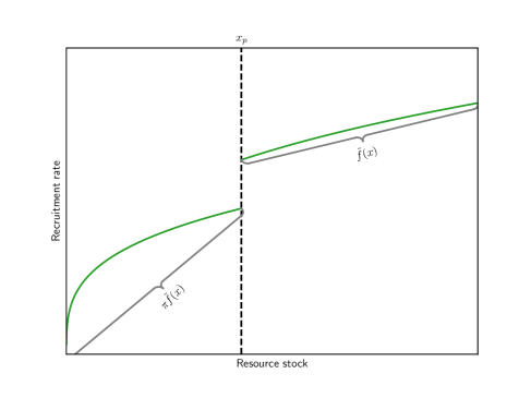
Figure 1: Tipping recruitment

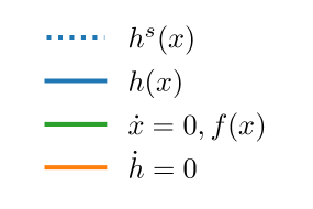
Legend for Figures˜1, 2, 3, 4, 6, 7 and 8

In particular, I define the tipping recruitment function as:

$$f(x)=\begin{cases}\pi\tilde{f}(x)&\text{if }x<x_{p}\\ \tilde{f}(x)&\text{if }x\geq x_{p}\end{cases}$$ (1)

where $f(x)$ is the natural growth rate of the resource stock for $x\geq 0$. The tipping point is $x_{p}>0$ and the tipping penalty is $0<\pi<1$. Below $x_{p}$, recruitment has low fecundity (the lower portion of Figure 1) and above, recruitment has high fecundity (the upper portion of Figure 1). The function $\tilde{f}$ is strictly increasing, twice differentiable, concave, $\tilde{f}(0)=0$, $\lim_{x\rightarrow 0}\tilde{f}^{\prime}(x)=\infty$ and $\lim_{x\rightarrow\infty}\tilde{f}^{\prime}(x)=0$.

At time $t$, if $x_{t}$ is the resource stock and $h_{t}$ is the harvest rate then the growth rate of the resource stock is:

$$\dot{x}_{t}=f(x_{t})-h_{t}.$$ (2)

Net resource growth, $\dot{x}_{t}$, is the natural rate at which the resource grows, $f(x_{t})$, less the harvest rate, $h_{t}$. When the harvest rate is below the recruitment rate ($h_{t}<f(x_{t})$), the resource stock is rising and when the harvest rate exceeds the recruitment rate ($h_{t}>f(x_{t})$), the resource stock is falling. At every time $t$, the resource stock and the harvest rate must be non-negative so that $x_{t}\geq 0$ and $h_{t}\geq 0$.

Given harvest rate, $h_{t}$ for $t\geq 0$, the discounted social welfare is given by:

$$\int_{0}^{\infty}e^{-\rho t}u(h_{t})dt$$ (3)

where $\rho>0$ is the social discount rate and $u(h_{t})$ is instantaneous social welfare. Let $u$ be a CRRA instantaneous social welfare function:

$$u(h)=\begin{cases}\frac{h^{1-\sigma}}{1-\sigma}&\text{if }\sigma\neq 1\\ \ln h&\text{if }\sigma=1\end{cases};$$ (4)

$\sigma>0$ is the coefficient of relative risk aversion and its inverse, $\sigma^{-1}$, is the elasticity of intertemporal substitution.

An optimal harvest plan solves:

$$\begin{gathered}V(x_{0})=\max_{h_{t}\geq 0}\int_{0}^{\infty}e^{-\rho t}u(h_{t})dt\\ \text{s.t.\ }\dot{x}_{t}=f(x_{t})-h_{t}\\ x_{t}\geq 0\\ \text{given }x_{0}>0\end{gathered}$$ (5)

where $x_{0}$ is the initial resource stock. The analysis of this otherwise standard problem is complicated by the discontinuity in $f$.

The current value Hamiltonian for this problem is:

$$\mathcal{H}(x,h,\lambda)=u(h)+\lambda[f(x)-h]$$ (6)

where $\lambda$ is the costate which represents the value of an infinitessimal increase in the resource stock, $x$. I will proceed to the analysis of (6) in Section˜3. In discussing trajectories (optimal and otherwise), it will be useful to refer to the policy function analogue, $h(x)$, that dictates the harvest rate when the resource stock is $x$.

2.1 Smooth recruitment

Before proceeding, I briefly review the analysis for the simpler case where there is no tipping point and the recruitment function is continuous. In particular, consider the recruitment function, $A\tilde{f}(x)$ where $A>0$. The solution to (6) satisfies the following necessary conditions:

$$h^{-\sigma}=\lambda,$$ (7)

$$\dot{\lambda}=\lambda[\rho-A\tilde{f}^{\prime}(x)],$$ (8)

$$\dot{x}=A\tilde{f}(x)-h.$$ (9)

Differentiating (7) with respect to $t$ and using (8) yields:

$$\dot{h}=\frac{1}{\sigma}h[A\tilde{f}^{\prime}(x)-\rho].$$ (10)

This implies that the optimal harvest rate is increasing over time when the marginal recruitment rate exceeds the social discount rate ($A\tilde{f}^{\prime}(x)>\rho$) and declining when the marginal recruitment rate is less than the social discount rate ($A\tilde{f}^{\prime}(x)<\rho$). A transversality condition,

$$\lim\limits_{t\rightarrow\infty}e^{-\rho t}\lambda_{t}x_{t}=0$$ (11)

implies that the discounted value of the resource stock is zero in the limit and ensures that harvests are optimal over the entire time horizon.

Figure 2: Smooth recruitment optimal harvest

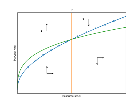
(a)

Together (9) and (10) represent an autonomous system of first-order differential equations that governs the model’s dynamics. Since $\mathcal{H}$ is strictly concave in $(x,h)$, together with (11), there is a unique solution, $(\hat{x}_{t}^{c},\hat{h}_{t}^{c})$, that converges to steady-state $(\hat{x}^{c},\hat{h}^{c})$ (Figure˜2). Let $\hat{h}^{c}(x)$ and $V^{c}(x)$ denote the corresponding policy and value functions. The superscript $c$ denotes variables and functions associated with the continuous problem.

Remark.

Both here and subsequently, $x$ and $h$ variables with time subscripts are trajectories, an $h$ with a functional argument is a policy function and a “hat” denotes optimality. A “hat” variable with no time subscript or functional argument is an optimal stationary point.

2.2 Austerity

It will be useful for the analysis of tipping points to compare trajectories and policies to one another. To do so, I define the notion of “austerity.”

Taking $A=\pi,1$, let $\underline{f}(\cdot)=\pi\tilde{f}(\cdot)$ and $\overline{f}(\cdot)=\tilde{f}(\cdot)$ be continuous low- and high-fecundity, recruitment functions and denote the corresponding current value Hamiltonians as $\underline{\mathcal{H}}$ and $\overline{\mathcal{H}}$. Given $x_{0}$, let the unique, optimal trajectories be given by $(\hat{\underline{x}}_{t},\hat{\underline{h}}_{t})$ and $(\hat{\overline{x}}_{t},\hat{\overline{h}}_{t})$ for $t\geq 0$. These trajectories converge to steady-states $(\hat{\underline{x}},\hat{\underline{h}})$ and $(\hat{\overline{x}},\hat{\overline{h}})$ and have corresponding policy functions $\hat{\underline{h}}(x)$ and $\hat{\overline{h}}(x)$ and value functions $\underline{V}(x)$ and $\overline{V}(x)$. Since $\pi<1$, it must be that $\hat{\underline{h}}(x)<\hat{\overline{h}}(x)$ and $\underline{V}(x)<\overline{V}(x)$. Call $(\hat{\underline{x}},\hat{\underline{h}})$ and $(\hat{\overline{x}},\hat{\overline{h}})$ the low and high notional steady-states. Define the “standard” policy function:

$$h^{s}(x)=\begin{cases}\hat{\underline{h}}(x)&\text{if }x<x_{p}\\ \hat{\overline{h}}(x)&\text{if }x\geq x_{p}\end{cases}.$$ (12)

I now define “austerity.” Loosely speaking, a trajectory $(x_{t},h_{t})$ is austere if it lies below the standard policy, $h^{s}(x)$. To be precise:

Definition 1.

Harvest policy $h(x)$ is austere relative to $h^{0}(x)$ if $h(x)\leq h^{0}(x)$ and there is $x^{\prime}<x^{\prime\prime}$ such that when $x\in[x^{\prime},x^{\prime\prime})$, $h(x)<h^{0}(x)$.

Definition 2.

Trajectory $(x_{t},h_{t})$ is austere relative to harvest policy $h^{0}(x)$ if the corresponding harvest policy, $h(x)$, defined over the domain $[\inf\{x_{t}\}_{t=0}^{\infty},$ $\sup\{x_{t}\}_{t=0}^{\infty}]$ is austere relative to $h^{0}(x)$ over the same domain.

Definition 3.

A harvest policy $h(x)$ or a trajectory $(x_{t},h_{t})$ is austere if it is austere relative to $h^{s}(x)$.

We will see that under the tipping recruitment function, $f(x)$, the optimal trajectory, $(\hat{x}_{t},\hat{h}_{t})$, may be austere.

3 Optimal harvest

I solve the discontinuous renewable resource problem by construction. I begin with the solution to the problem where $x_{0}\geq x_{p}$ and assume that the resource stock is constrained to remain at or above the tipping point. The solution to this problem will yield a constrained optimal path, $(\hat{x}_{t}^{*},\hat{h}_{t}^{*})$, that converges to $(\hat{x}^{*},\hat{h}^{*})$. For $x\geq x_{p}$, the corresponding harvest policy and value functions are $\hat{h}^{*}(x)$ and $V^{*}(x)$.

Next, I solve the problem for $x_{0}<x_{p}$, allowing for the possibility that the optimal trajectory may transition to the high-fecundity recruitment function. For a given initial resource stock, $x_{0}$, this has two possible solutions: i) the optimal trajectory, $(\hat{x}_{*t},\hat{h}_{*t})$, converges to the low notional stationary point, $(\hat{x}_{*},\hat{h}_{*})=(\hat{\underline{x}},\hat{\underline{h}})$ or ii) the optimal trajectory reaches the tipping point so that $\hat{x}_{*T}=x_{p}$ at time $T$ with terminal value $e^{-\rho T}V^{*}(x_{p})$, under the assumption that harvests thereafter follow the constrained, high-fecundity solution that converges to $(\hat{x}^{*},\hat{h}^{*})$.

Finally, given these solutions, I show that when high-fecundity is sufficiently valuable, the constrained, high-fecundity solution is still optimal when $x_{t}$ is allowed to fall below $x_{p}$. Consequently, the solution to the low-fecundity problem is also optimal.

3.1 Constrained high-fecundity problem

Consider the problem where the resource stock is constrained to stay at or above the tipping point:

$$\begin{gathered}V^{*}(x_{0})=\max_{h_{t}\geq 0}\int_{0}^{\infty}e^{-\rho t}u(h_{t})dt\\ \text{s.t.\ }\dot{x}_{t}=\tilde{f}(x_{t})-h_{t}\\ x_{t}\geq x_{p}\\ \text{given }x_{0}\geq x_{p}.\end{gathered}$$ (13)

This is problem (5) for $x_{0}\geq x_{p}$ where there is the additional constraint that $x_{t}\geq x_{p}$ for all $t\geq 0$.

Figure 3: Constrained upper problem

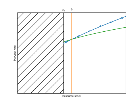
(a) Interior

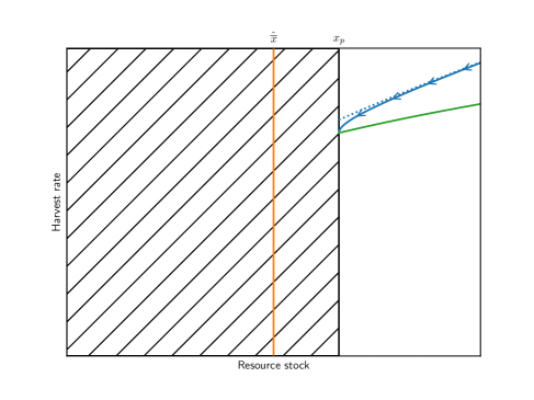
(b) Boundary

Proposition 1.

For the high-fecundity problem given by (13), the optimal trajectory, $(\hat{x}_{t}^{*},\hat{h}_{t}^{*})$ for all $t\geq 0$, is unique and:

1. if $\hat{\overline{x}}\geq x_{p}$ then $(\hat{x}_{t}^{*},\hat{h}_{t}^{*})=(x_{t}^{s},h_{t}^{s})$ and $\hat{x}^{*}=\hat{\overline{x}}$,

2. if $\hat{\overline{x}}<x_{p}$ then $(\hat{x}_{t}^{*},\hat{h}_{t}^{*})$ is austere and there is some time $\tau<\infty$ such that for all $t\geq\tau$, $\hat{x}_{t}^{*}=x_{p}$.

The proof of Proposition˜1 and all subsequent proofs are in given in Appendix A.

When the high notional stationary point is at least the tipping point ($\hat{\overline{x}}\geq x_{p}$), the constraint is non-binding and the optimal policy corresponds to the standard policy and the constrained optimal stationary point corresponds to the high notional stationary point defined in Section˜2.2 (Figure˜3a).

But if the high notional stationary point is below the tipping point ($\hat{\overline{x}}<x_{p}$), the constraint is strictly binding and the optimal harvest is austere with the resource stock falling and stopping at $x_{\tau}=x_{p}$ at time $\tau$ (Figure˜3b). To see this, when the harvest trajectory is not sufficiently austere, the resource stock reaches the tipping point too quickly. On the other hand, when the harvest trajectory is too austere, the trajectory crosses the $\dot{x}=0$ line and is suboptimal since harvesting $\tilde{f}(x_{p})$ is always feasible.

3.2 Low-fecundity problem

Now consider the low fecundity problem where $x_{0}<x_{p}$. Assume that if a trajectory, $(x_{t},h_{t})$, reaches the tipping point $x_{p}$ at some time $T$, then the terminal payoff is $e^{-\rho T}V^{*}(x_{p})$. Beyond time $T$, the trajectory is assumed to follow the solution from Section˜3.1.

While it is always possible for the resource stock to reach $x_{p}$, it may not be optimal. Thus there are two candidate outcomes. In one outcome, high-fecundity is not attained and the resource stock converges to the low notional steady-state, $\hat{\underline{x}}$. In the second outcome, the resource stock increases until it reaches the tipping point, $x_{p}$, whereupon recruitment becomes high-fecundity at time $T$.

The optimization problem for the latter type of outcome is:

$$\begin{gathered}V_{2}(x_{0})=\max_{h_{t}\geq 0}\int_{0}^{T}e^{-\rho t}u(h_{t})dt+e^{-\rho T}V^{*}(x_{p})\\ \text{s.t. }\dot{x}_{t}=\pi\tilde{f}(x_{t})-h_{t}\\ x_{t}\geq 0\\ x_{T}=x_{p}\\ T\text{ free}\\ \text{given }x_{0}<x_{p}.\end{gathered}$$ (14)

This is a control problem with fixed terminal point, $x_{p}$, “scrap value,” $e^{-\rho T}V^{*}(x_{p})$ and free terminal time, $T$.

Either type of outcome must solve the current value Hamiltonian (6) so that both must satisfy (9) and (10) where $f(x)=\pi\tilde{f}(x)$ and $f^{\prime}(x)=\pi\tilde{f}^{\prime}(x)$. In addition, optimal trajectories must satisfy the appropriate transversality conditions. For the outcome that converges to the low notional stationary point, this is the standard transversality condition (11). For the outcome that transitions to high-fecundity at time $T$, the transversality condition is:

$$\lim_{t\rightarrow T}\underline{\mathcal{H}}(x_{t},h_{t},\lambda_{t})=\rho V^{*}(x_{p}).$$ (15)

This has the intuitive interpretation that as $t\rightarrow T$, the flow value of trajectory $(x_{t},h_{t})$, as represented by the current value Hamiltonian, must be equal to the flow value of the terminal payoff, $\rho V^{*}(x_{p})$. Since $h_{t}<\pi\tilde{f}(x_{t})$, Lemma˜2 from the Appendix shows that $\underline{\mathcal{H}}(x,h,u^{\prime}(h))$ is decreasing in $h$ and implies that if $\lim_{t\rightarrow T}\underline{\mathcal{H}}(x_{t},h_{t},\lambda_{t})>\rho V^{*}(x_{p})$ then high-fecundity is being attained too quickly so that $(x_{t},h_{t})$ is overly austere and larger harvests would be welfare improving. Conversely, if $\lim_{t\rightarrow T}\underline{\mathcal{H}}(x_{t},h_{t},\lambda_{t})<\rho V^{*}(x_{p})$ then the transition to high-fecundity is too slow and $(x_{t},h_{t})$ is insufficiently austere so that smaller harvests are optimal.

The overall solution to the low-fecundity problem will have an endogenous tipping (Skiba) point, below which the standard trajectory obtains and above which an austere trajectory reaching $x_{p}$ and high fecundity is attained.

Proposition 2.

For the low-fecundity problem, if $\hat{\underline{h}}(x_{p})\leq\tilde{f}(x_{p})$ then the optimal trajectory, $(\hat{x}_{*t},\hat{h}_{*t})$ for all $t\geq 0$, is unique and there exists $x_{p}^{\prime}\in[0,x_{p})$ such that

1. if $x_{0}<x_{p}^{\prime}$ then $(\hat{x}_{*t},\hat{h}_{*t})=(x_{t}^{s},h_{t}^{s})$ and $\hat{x}_{*}=\hat{\underline{x}}$,

2. if $x_{0}\geq x_{p}^{\prime}$ then $(\hat{x}_{*t},\hat{h}_{*t})$ is austere and there is some time $\tau<\infty$ such that $\hat{x}_{*\tau}=x_{p}$.

In particular, provided that $\hat{\underline{h}}(x_{p})\leq\tilde{f}(x_{p})$, there is an endogenous tipping point, $x_{p}^{\prime}$ (possibly trivial with $x_{p}^{\prime}=0$). Above $x_{p}^{\prime}$, the optimal trajectory is austere and at time $\tau$, $\hat{x}_{*\tau}=x_{p}$ and thereafter, the optimal trajectory follows the high-fecundity solution from Section˜3.1. Below $x_{p}^{\prime}$, austerity is too costly and the optimal harvest is the standard policy which converges to the low notional steady-state, $\hat{\underline{x}}$.

The condition that $\hat{\underline{h}}(x_{p})\leq\tilde{f}(x_{p})$ implies that high-fecundity is relatively valuable, ensuring the existence of an optimal, austere harvest policy that transitions the ecosystem to high-fecundity. The following Proposition provides sufficient conditions.

Proposition 3.

If $\pi$, $\rho$ and $x_{p}$ are sufficiently small then $\hat{\underline{h}}(x_{p})\leq\tilde{f}(x_{p})$.

When the conditions of Proposition˜3 hold, the value of the terminal payoff, $e^{-\rho T}V^{*}(x_{p})$, is high and austere harvests can optimally attain high fecundity. Otherwise, high fecundity is not sufficiently attractive and the planner prefers the low-fecundity, standard harvest policy.

3.3 Unconstrained optimality

Now consider the full problem where the resource stock is only constrained to be non-negative. In particular, for $x_{0}\geq x_{p}$, an unconstrained trajectory can have $x_{t}<x_{p}$ for some $t>0$. Let $(\hat{x}_{t},\hat{h}_{t})$ be the trajectory that solves this problem with corresponding policy function, $\hat{h}(x)$, and value function, $V(x)$.

Proposition 4.

For the unconstrained problem, if $\pi$, $\rho$ and $x_{p}$ are sufficiently small then the optimal trajectory, $(\hat{x}_{t},\hat{h}_{t})$ for all $t\geq 0$, is unique and there exists $x_{p}^{\prime}\in[0,x_{p})$ such that

1. if $x_{0}\in(0,x_{p}^{\prime})$ then the optimal trajectory is $(\hat{x}_{t},\hat{h}_{t})=(x_{t}^{s},h_{t}^{s})$ and $\hat{x}=\hat{\underline{x}}$,

2. if $x_{0}\in[x_{p}^{\prime},x_{p})$ then the optimal trajectory $(\hat{x}_{t},\hat{h}_{t})$ is austere and there exists $\tau<\infty$ such that $\hat{x}_{\tau}=x_{p}$ and $\hat{x}=\max\{\hat{\overline{x}},x_{p}\}$,

3. if $x_{0},\hat{\overline{x}}\geq x_{p}$ then $(\hat{x}_{t},\hat{h}_{t})=(\hat{x}_{t}^{s},\hat{h}_{t}^{s})$ and $\hat{x}=\hat{\overline{x}}$,

4. if $x_{0}\geq x_{p}>\hat{\overline{x}}$ then $(\hat{x}_{t},\hat{h}_{t})$ is austere and there exists $\tau<\infty$ such that $\hat{x}_{t}=x_{p}$ for $t\geq\tau$.

When $\pi$, $\rho$ and $x_{p}$ are small, high-fecundity is relatively valuable and the planner prefers high-fecundity to low-fecundity.

Above the tipping point ($x_{0}\geq x_{p}$) there is a stable, high-fecundity steady-state. When $\hat{\overline{x}}>x_{p}$, the tipping point is strictly non-binding so that $(\hat{x}_{t},\hat{h}_{t})=(\hat{x}_{t}^{s},\hat{h}_{t}^{s})$ and the ecosystem converges to the notional, high-fecundity stationary point ($\hat{x}=\hat{\overline{x}}$) (Figures˜4a, 4b, 4c, 4d, 4e and 4f). But if $\hat{\overline{x}}<x_{p}$, then the high-fecundity steady-state occurs at the tipping point and $\hat{x}=x_{p}$. In order to reach this steady-state optimally, harvests must be austere; the standard harvest policy brings the resource stock to the tipping point too quickly. Even though the stationary resource stock $\hat{x}=x_{p}$ is stable, a small perturbation can result in a large fall in both harvests and recruitment (Figures˜5a, 5b and 5c).

Figure 4: Optimal harvest policies

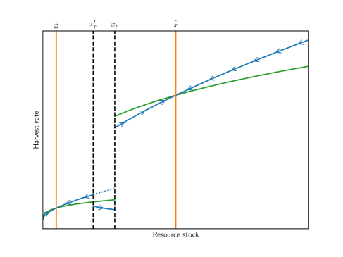
(a) Low Tipping Point, Low $\pi$

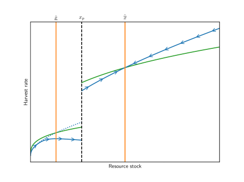
(b) Low Tipping Point, Med $\pi$

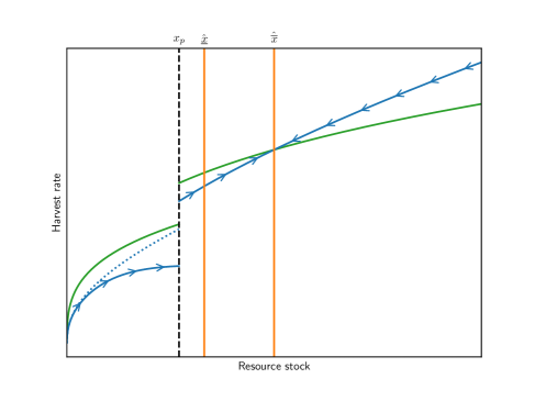
(c) Low Tipping Point, High $\pi$

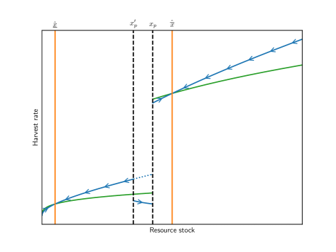
(d) Med Tipping Point, Low $\pi$

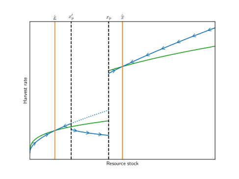
(e) Med Tipping Point, Med $\pi$

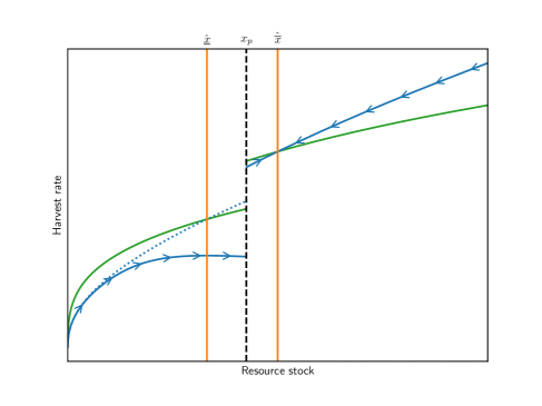
(f) Med Tipping Point, High $\pi$

Figure 5: Optimal harvest policies (continued)

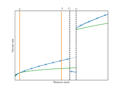
(a) High Tipping Point, Low $\pi$

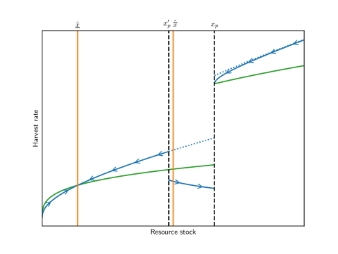
(b) High Tipping Point, Med $\pi$

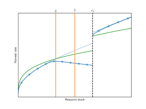
(c) High Tipping Point, High $\pi$

Below the tipping point ($x_{0}<x_{p}$), there is an endogenous tipping point, $x_{p}^{\prime}$. For $x_{0}<x_{p}^{\prime}$, the cost of austerity is too high and recovery, while feasible, is suboptimal; instead the resource stock converges to the low-fecundity stationary point and $\hat{x}=\hat{\underline{x}}$ (Figures˜4a, 4d, 4e, 5a and 5b). That is, given model parameters, below this endogenous tipping point, an austere harvest policy is inferior to the standard policy. For $x_{0}\geq x_{p}^{\prime}$, austerity does not need to be borne for long and the optimal harvest transitions the renewable resource to high-fecundity and $\hat{x}\geq x_{p}$.

Finally, it may be that the endogenous tipping point is inconsequential ($x_{p}^{\prime}=0$). When the low notional steady-state is infeasible ($\hat{\underline{x}}>x_{p}$) (Figure˜4c) or when the high-/low-fecundity differential is relatively small (Figures˜4b, 4f and 5c) then there is no non-trivial low steady-state. In these cases, as long as $x_{0}>0$, the optimal trajectory always reaches the high-fecundity steady-state and $\hat{x}=\max\{\hat{\overline{x}},x_{p}\}$. Despite the potential nonexistence of a bad long term outcome, as practitioners, we will be more interested in parameter configurations where the tipping point has a significant and tangible impact.

Figure 6: Large $\pi$, $\rho$ and $x_{p}$

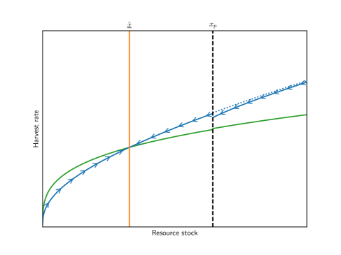
(a) Large $\pi$, $x_{p}$

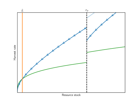
(b) Large $\rho$, $x_{p}$

When the conditions of Proposition˜3 fail, there is no high-fecundity steady-state (Figure˜6). Since the high notional steady-state is always preferable to the low notional steady-state, when these conditions fail, it must be the case that the high notional steady-state is infeasible and $\hat{\overline{x}}<x_{p}$. Examples of the failure of Proposition˜3 are illustrated in Figure˜6a where $\pi$ is close to 1 and in Figure˜6b where $\rho$ is large. Notice that at high-fecundity ($x_{0}>x_{p}$), optimal harvests are austere in order prolong high-fecundity prior to the eventual transition to low-fecundity. The formal analysis of this case would first solve the low-fecundity problem under the assumption that the resource stock can never exceed the tipping point ($x_{t}<x_{p}$). Then, taking this solution as given, solve the high-fecundity problem where $x_{0}\geq x_{p}$ where the planner may choose to tip the ecosystem. Aside from this basic sketch, I do not formally analyze the case where there is no high-fecundity steady-state.

4 Hysteresis

In recent years there is evidence that recovery from environmental damage can be subject to hysteresis (Field et al. 2007; Storlazzi et al. 2009 for coral reefs, Lindig-Cisneros et al. 2003 for wetlands, Hirota et al. 2011 for rain forests). Hysteresis has become an important factor that marine ecologists consider as they seek to understand tipping points (Selkoe et al., 2015).

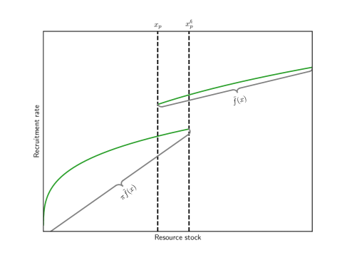
Figure 7: Hysteretic tipping recruitment

When recruitment is subject to hysteresis, there are two tipping points. If fecundity is high then the tipping point is given by $x_{p}$. If the resource stock falls below this tipping point, the renewable resource switches to low-fecundity. With hysteresis, a higher tipping point must be reached in order for the renewable resource to transition to high-fecundity; the low-fecundity tipping point is given by $x_{p}^{\mathcal{h}}>x_{p}$. Functionally, the hysteretic recruitment function has a second argument, $s$:

$$f(x,s)=(1-s)\pi\tilde{f}(x)+s\tilde{f}(x)$$

where $s\in\{0,1\}$ is the ecosystem’s state with $s=1$ representing high-fecundity and $s=0$ low-fecundity. For $x<x_{p}$, $s=0$, for $x\geq x_{p}^{\mathcal{h}}$, $s=1$ and for $x\in[x_{p},x_{p}^{\mathcal{h}})$, $\dot{s}=0$ (i.e., $s$ retains its value). Recruitment can change discontinuously at $x_{p}$ and $x_{p}^{\mathcal{h}}$ (Figure˜7).

In the model with hysteresis, denote the optimal trajectory $(\hat{x}_{t}^{\mathcal{h}},\hat{h}_{t}^{\mathcal{h}})$ with corresponding policy function, $\hat{h}^{\mathcal{h}}(x,s)$, and value function, $V^{\mathcal{h}}(x,s)$. With hysteresis,

Proposition 5.

If $\pi$, $\rho$ and $x_{p}^{\mathcal{h}}$ are sufficiently small then then the optimal trajectory, $(\hat{x}_{t}^{\mathcal{h}},\hat{h}_{t}^{\mathcal{h}})$ for $t\geq 0$, is unique and there exists $x_{p}^{\mathcal{h}\prime}\in[0,x_{p}^{\mathcal{h}})$ such that

1. if $x_{0}\in(0,x_{p}^{\mathcal{h}\prime})$ and $s_{0}=0$ then the optimal trajectory is $(\hat{x}_{t}^{\mathcal{h}},\hat{h}_{t}^{\mathcal{h}})=(\hat{x}_{t}^{s},\hat{h}_{t}^{s})$ and $\hat{x}^{\mathcal{h}}=\hat{\underline{x}}$,

2. if $x_{0}\in[x_{p}^{\mathcal{h}\prime},x_{p}^{\mathcal{h}})$ and $s_{0}=0$ then the optimal trajectory $(\hat{x}_{t}^{\mathcal{h}},\hat{h}_{t}^{\mathcal{h}})$ is austere and there exists $\tau<\infty$ such that $\hat{x}_{\tau}^{\mathcal{h}}=x_{p}^{\mathcal{h}}$ and $\hat{x}^{\mathcal{h}}=\max\{\hat{\overline{x}},x_{p}\}$

3. if $x_{0},\hat{\overline{x}}\geq x_{p}$ and $s_{0}=1$ then $(\hat{x}_{t}^{\mathcal{h}},\hat{h}_{t}^{\mathcal{h}})=(\hat{x}_{t}^{s},\hat{h}_{t}^{s})$ and $\hat{x}^{\mathcal{h}}=\hat{\overline{x}}$,

4. if $x_{0}\geq x_{p}>\hat{\overline{x}}$ and $s_{0}=1$ then $(\hat{x}_{t}^{\mathcal{h}},\hat{h}_{t}^{\mathcal{h}})$ is austere and there exists $\tau<\infty$ such that $\hat{x}_{t}^{\mathcal{h}}=x_{p}$ for $t\geq\tau$.

5. $x_{p}^{\prime}<x_{p}^{\mathcal{h}\prime}$.

As in the model without hysteresis, there is an endogenous tipping point. Above the endogenous tipping point, the cost of austerity is relatively low and the optimal harvest policy is austere and attains high-fecundity recruitment (Figure˜8). Since the low-fecundity tipping point is greater than the high-fecundity tipping point, upon reaching high-fecundity recruitment, the optimal harvest policy may then reverse course and spend down the resource stock to reach the high-fecundity steady-state (Figures˜8d, 8e, 8f, 9a, 9b and 9c). Below the endogenous tipping point, an austere harvest achieving high-fecundity recruitment is suboptimal and instead the optimal harvest follows the standard policy converging to the low-fecundity steady-state (Figures˜8a, 8b, 8d, 8e, 9a, 9b and 9c).

Figure 8: Hysteretic optimal harvest policies

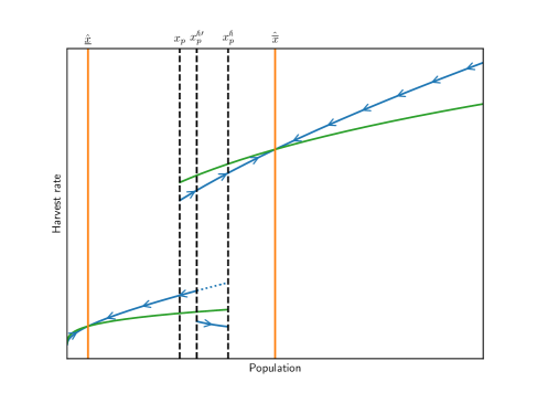
(a) Low Tipping Point, Low $\pi$

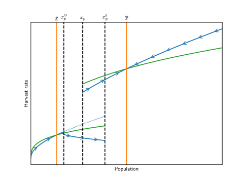
(b) Low Tipping Point, Med $\pi$

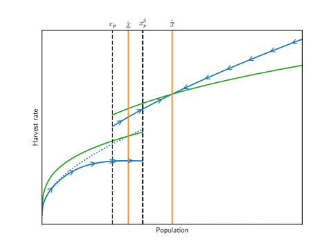
(c) Low Tipping Point, High $\pi$

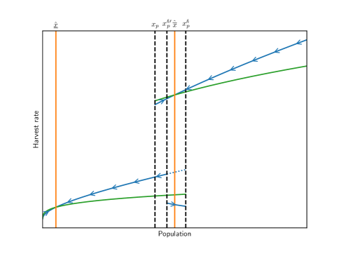
(d) Med Tipping Point, Low $\pi$

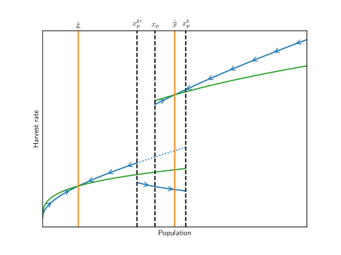
(e) Med Tipping Point, Med $\pi$

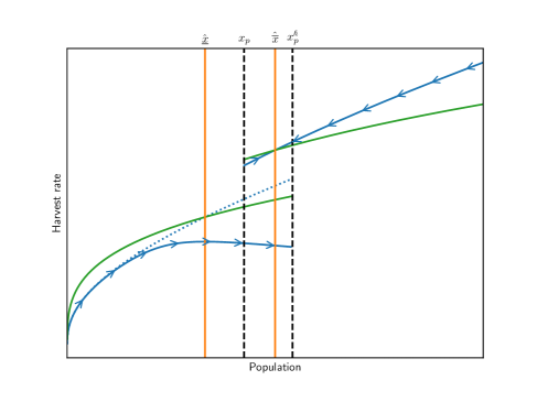
(f) Med Tipping Point, High $\pi$

Figure 9: Hysteretic optimal harvest policies (continued)

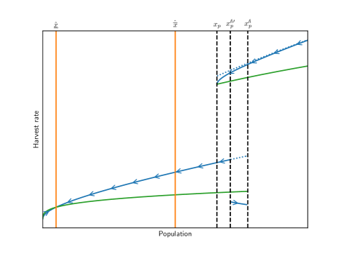
(a) High Tipping Point, Low $\pi$

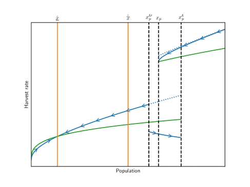
(b) High Tipping Point, Med $\pi$

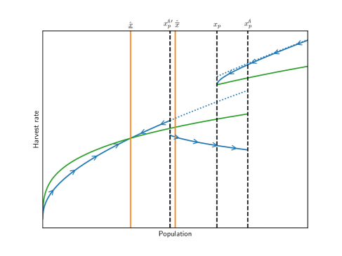
(c) High Tipping Point, High $\pi$

In contrast to the model without hysteresis, a high-fecundity steady-state at the high-fecundity tipping point is no longer stable. If the high and low-fecundity differential is not too large then a perturbation that drops the resource stock below the tipping point requires an extended recovery period to return to high-fecundity, whereupon the optimal harvest spends down the resource stock to return to the steady-state (Figures˜9b and 9c). However, if the high- and low-fecundity differential is large then the endogenous tipping point, $x_{p}^{\mathcal{h}\prime}$, may be greater than the exogenous, high-fecundity tipping point. While returning to high-fecundity recruitment is feasible, it is suboptimal so that a fall below the tipping point becomes permanent (Figure˜9a). That is, a high-fecundity stationary point that corresponds to the high-fecundity tipping point may not even be “long run stable.”

Finally, since $x_{p}^{\mathcal{h}\prime}>x_{p}^{\prime}$, with hysteresis, the range over which initial resource stocks optimally remains at low-fecundity is larger.

A disheartening example of the slow recovery from a renewable resource collapse is the case of the Atlantic northwest cod fishery of the early 1990s (Hutchings and Myers, 1994; Walters and Maguire, 1996). After more than three decades of restricted harvests, the Atlantic northwest cod fishery has still not recovered to sustainable levels (DFO, 2021, 2024) and the hoped for 2025 recovery (Rose and Rowe, 2015) appears unlikely to have come to fruition.

5 Conclusion

In this paper I characterized the optimal extraction of a renewable resource where recruitment is subject to tipping points. Historically, tipping points have been modeled using hazard models where tipping is irreversible. In contrast, with a fixed tipping point, I am able to model renewable resource recovery. Moreover, when ecosystem recovery is possible, it becomes straightforward to model and analyze hysteresis. To the best of my knowledge, I am the first to do both of these.

With endogenous reversibility, ecosystem recovery is not always optimal. When the ecosystem is sufficiently degraded, austerity becomes too costly and low fecundity becomes permanent. If in addition there is hysteresis, even a small perturbation that causes tipping may be permanent when the low-fecundity penalty is sufficiently severe. In this case, austerity may be too costly, even for an infinitesimal drop below the high-fecundity tipping point.

This analysis presents a cautionary tale. First, it demonstrates that when an ecosystem suffers sufficient degradation, the resulting damage is irreversible. Moreover, with hysteresis, even a small perturbation can trigger long-lasting and potentially permanent changes. This underscores the delicate balance of natural systems and the critical importance of conservation efforts to prevent crossing ecological tipping points.

In this paper, I presented an ideal scenario where a social planner has complete control over harvests, all features of the ecosystem are known with certainty and there are no spillovers with other resources. With more than one resource extractor (tragedy of the commons), remaining above the tipping point would be more challenging (Levhari and Mirman, 1980). Moreover, there may be important interactions between different renewable resources. For instance, deforestation results in the loss of habitat for native wildlife that may impact wildlife fecundity (Faria et al., 2023). Finally, uncertainty is important but has been left unmodeled. These complications, while important, are not considered here and call for further research.

Appendix

Appendix A Proofs

Proof of Proposition˜1.

i) For $\hat{\overline{x}}\geq x_{p}$, since $(\hat{\overline{x}}_{t},\hat{\overline{h}}_{t})$ is optimal in the absence of constraint, it is also optimal with the constraint $x_{t}\geq x_{p}$. Thus $(\hat{x}_{t}^{*},\hat{h}_{t}^{*})=(\hat{\overline{x}}_{t},\hat{\overline{h}}_{t})=(x_{t}^{s},h_{t}^{s})$ and $\hat{x}_{t}^{*}\rightarrow\hat{\overline{x}}$.

ii) For $\hat{\overline{x}}<x_{p}$, there are two classes of trajectories $(x_{t},h_{t})$ satisfying (9) and (10).

In one, $(x_{t},h_{t})$ crosses the $\dot{x}=0$ curve (the green line in fig.˜3b) at some point above $x_{p}$. Since $\hat{\overline{x}}<x_{p}$, the crossing point cannot be stationary ($\dot{h}_{t}<0$) and standard arguments show that $(x_{t},h_{t})$ is suboptimal.

In the second class, $(x_{t},h_{t})$ reaches $x_{T}=x_{p}$ at some time $T$. For such trajectories, upon reaching $x_{T}=x_{p}$, (9) and (10) imply that $(x_{t},h_{t})=(x_{p},\tilde{f}(x_{p}))$ for $t>T$, otherwise the constraint that $x_{t}\geq x_{p}$ would be violated. The optimal harvest problem can thus be rewritten as a free-terminal-time problem with terminal value, $e^{-\rho T}u(\tilde{f}(x_{p}))/\rho$:

$$\begin{gathered}V^{*}(x_{0})=\max_{h_{t}\geq 0}\int_{0}^{T}e^{-\rho t}u(x_{t})dt+e^{-\rho T}\frac{u(\tilde{f}(x_{p}))}{\rho}\\ \text{s.t. }\dot{x}_{t}=\tilde{f}(x_{t})-h_{t}\\ x_{t}\geq x_{p}\\ T\text{ free}\\ \text{given }x_{0}\geq x_{p}\end{gathered}$$

where the transversality condition is

$$\overline{\mathcal{H}}(x_{T},h_{T},\lambda_{T})=u(\tilde{f}(x_{p})).$$ (A.1)

But $u(h_{T})+\lambda_{T}[\tilde{f}(x_{p})-h_{T}]=u(\tilde{f}(x_{p}))$ if and only if $h_{T}=\tilde{f}(x_{p})$. Therefore, for $t<T$, $(\hat{x}_{t}^{*},\hat{h}_{t}^{*})$ is such that $\lim_{t\rightarrow T}\hat{h}_{t}^{*}=\tilde{f}(x_{p})$ and for $t\geq T$ $(\hat{x}_{t}^{*},\hat{h}_{t}^{*})=(x_{p},\tilde{f}(x_{p}))$. Let $\tau=T$. Since $(\hat{x}_{t}^{*},\hat{h}_{t}^{*})$ is the only trajectory satisfying (A.1), the solution is unique.

Now consider trajectory $(x_{t}^{s},h_{t}^{s})$ that corresponds to the standard policy $h^{s}(\cdot)$ for a given $x_{0}$ (dotted blue line in Figure˜3b). In the continuous, high-fecundity problem, $x_{t}^{s}\rightarrow\hat{\overline{x}}$ from above so that at some time $T^{\prime}$, $x^{s}_{T^{\prime}}=x_{p}$ and $h_{T^{\prime}}^{s}>\tilde{f}(x_{p})$. Therefore, $(\hat{x}_{t}^{*},\hat{h}_{t}^{*})$ and is austere. ∎

Lemma 1.

For the constrained high fecundity problem, $V^{*}(x)\geq\frac{u(\tilde{f}(x_{p}))}{\rho}$.

Proof.

Since $\tilde{f}$ is strictly increasing, if $x_{t}\geq x_{p}$ for any $t\geq 0$ then harvesting $\tilde{f}(x_{p})$ is always feasible but not necessarily optimal. Therefore

$$V^{*}(x_{0}) =\int_{0}^{\infty}e^{-\rho t}u(\hat{h}_{t}^{*})dt$$

$$\geq\int_{0}^{\infty}e^{-\rho t}u(\tilde{f}(x_{p}))dt$$

$$=\frac{u(\tilde{f}(x_{p}))}{\rho}.$$

∎

Lemma 2.

$$\mathcal{H}(x,h,u^{\prime}(h))=u(h)+u^{\prime}(h)[A\tilde{f}(x)-h]$$

is strictly decreasing in $h$ when $h<A\tilde{f}(x)$ and strictly increasing in $h$ when $h>A\tilde{f}(x)$.

Proof.

Differentiating with respect to $h$,

$$\frac{\partial\mathcal{H}(x,h,u^{\prime}(h))}{\partial h}=u^{\prime\prime}(h)[A\tilde{f}(x)-h].$$

Since $u^{\prime\prime}(h)<0$, this is negative when $h<A\tilde{f}(x)$ and positive when $h>A\tilde{f}(x)$. ∎

Proof of Proposition˜2.

The plan of the proof is to: 1. Characterize candidate optimal trajectories: a) $(x_{1t},h_{1t})$ such that $\lim_{t\rightarrow\infty}(x_{1t},h_{1t})=(\hat{\underline{x}},\hat{\underline{h}})$ and b) $(x_{2t},h_{2t})$ where there exists some $\tau>0$ such that $x_{2\tau}=x_{p}$, 2. Show that $(x_{2t},h_{2t})$ is austere and 3. Show that there is an endogenous tipping point, $x_{p}^{\prime}$, below which $(x_{1t},h_{1t})$ is optimal and above which $(x_{2t},h_{2t})$ is optimal.

1. 1. Begin by considering trajectories, $(x_{1t},h_{1t})$, that converge to the low notional steady-state, $(\hat{\underline{x}},\hat{\underline{h}})$.

      If $\hat{\underline{x}}<x_{p}$ then the standard analysis shows that for $x_{0}<x_{p}$, $(\hat{\underline{x}}_{t},\hat{\underline{h}}_{t})$ is the unique trajectory satisfying (9), (10) and (11) and converges to $(\hat{\underline{x}},\hat{\underline{h}})$. Let $(x_{1t},h_{1t})=(\hat{\underline{x}}_{t},\hat{\underline{h}}_{t})$ and denote the corresponding value function $V_{1}(x)=\underline{V}(x)$.

      If $\hat{\underline{x}}\geq x_{p}$ then $\hat{\underline{x}}$ is not feasible and cannot be a steady-state. Therefore there is no trajectory satisfying (9), (10) and (11) that converges to $(\underline{\hat{x}},\underline{\hat{h}}))$ (see fig.˜4c).

   2. Now consider a trajectory $(x_{t},h_{t})$ such that at some time $T$, $x_{T}=x_{p}$. In order to reach $x_{p}$ from $x_{0}<x_{p}$, it must be that $\dot{x}_{t}>0$. Equation (9) implies that $h_{t}<\pi\tilde{f}(x_{t})$ and consequently, $\lim_{t\rightarrow T}h_{t}\leq\pi\tilde{f}(x_{p})$; let $h_{T}^{-}=\lim_{t\rightarrow T}h_{t}$. Upon reaching $x_{T}=x_{p}$, the terminal payoff is $e^{-\rho T}V^{*}(x_{p})$.

      Given the terminal payoff $e^{-\rho T}V^{*}(x_{p})$, the optimal trajectory minimizes the time required to reach $x_{p}$ while not sacrificing too much through austere early harvests. This balance is captured by the free-stopping-time transversality condition, (15).

      For $h=\pi\tilde{f}(x_{p})$,

      $$\underline{\mathcal{H}}(x_{p},h,\lambda) =u(\pi\tilde{f}(x_{p}))$$

      $$<u(\tilde{f}(x_{p}))=\rho\frac{u(\tilde{f}(x_{p}))}{\rho}$$

      $$\leq\rho V^{*}(x_{p}).$$ Lemma˜1

      Since, $\lim_{h\rightarrow 0}h^{1-\sigma}/(1-\sigma)+\pi\tilde{f}(x_{p})h^{-\sigma}=\infty$, $\lim_{h\rightarrow 0}\underline{\mathcal{H}}(x_{p},h,u^{\prime}(h))=\infty$. Continuity implies that there is at least one $h_{T}^{-}$ such that (15) is satisfied.

      From Lemma˜2, if $h<\pi\tilde{f}(x)$ then $\underline{\mathcal{H}}(x,h,u^{\prime}(h))$ is strictly decreasing in $h$. Therefore there is a unique $h_{T}^{-}\in(0,\pi\tilde{f}(x_{p}))$ such that (9), (10) and (15) hold. Let $(x_{2t},h_{2t})$ be the trajectory satisfying (9), (10), (15) such that $x_{2T}=x_{p}$. Let $\tau=T$.

2. To show that $(x_{2t},h_{2t})$ is austere, consider two cases: a) $\hat{\underline{x}}\geq x_{p}$ and b) $\hat{\underline{x}}<x_{p}$.

   1. For $\hat{\underline{x}}\geq x_{p}$, we know that $\hat{\overline{x}}>x_{p}$ so that the standard analysis holds for the high-fecundity problem and $\hat{h}^{*}(x_{p})=\hat{\overline{h}}(x_{p})$ and $V^{*}(x_{p})=\overline{V}(x_{p})$. Since $\overline{V}(x)>\underline{V}(x)$ it follows that:

      $$\underline{\mathcal{H}}(x_{p},h_{2\tau}^{-},u^{\prime}(h_{2\tau}^{-})) =\rho V^{*}(x_{p})$$ transversality (A.2)

      $$=\rho\overline{V}(x_{p})$$

      $$>\rho\underline{V}(x_{p})$$

      $$=\underline{\mathcal{H}}(x_{p},\hat{\underline{h}}(x_{p}),u^{\prime}(\hat{\underline{h}}(x_{p}))) \text{HJB}.$$

      where $h_{2\tau}^{-}=\lim_{t\rightarrow\tau}h_{2t}$. It was shown above that $h_{2\tau}^{-}\leq\pi\tilde{f}(x_{p})$ and since $\hat{\underline{x}}\geq x_{p}$, the low notional stationary point is not feasible and $\hat{\underline{h}}(x_{p})\leq\pi\tilde{f}(x_{p})$. Since $\underline{\mathcal{H}}(x_{p},h,u^{\prime}(h))$ is decreasing in $h$ when $h\leq\pi\tilde{f}(x)$ (Lemma˜2), it must be that $h_{2\tau}^{-}<\hat{\underline{h}}(x_{p})$. Therefore, $(x_{2t},h_{2t})$ is austere.

   2. For $\hat{\underline{x}}<x_{p}$, if $x_{0}\in(\hat{\underline{x}},x_{p})$ then the low-fecundity optimal resource stock, $\hat{\underline{x}}_{t}$, converges to $\hat{\underline{x}}$ from above (see dotted blue trajectories from figs.˜4a, 4b, 4d, 4e, 4f, 5a, 5b and 5c) so that $\hat{\underline{h}}(x)>\pi\tilde{f}(x)$ for $x\in(\hat{\underline{x}},x_{p})$. But we know that $(x_{2t},h_{2t})$ leads to $x_{2\tau}=x_{p}$ and must have $h_{2t}<\pi\tilde{f}(x_{2t})$ (follows from $\dot{x}_{2t}>0$). Therefore, $\hat{\underline{h}}(x_{2t})>h_{2t}$ and $(x_{2t},h_{2t})$ is austere.

3. There are two candidate optimal trajectories and it remains to be determined when $(x_{1t},h_{1t})$ is optimal and when $(x_{2t},h_{2t})$ is optimal.

   For any trajectory, $(x_{t},h_{t})$, satisfying (9) and (10), take the ratio of (10) and (9) to get an expression representing the slope of the corresponding policy function:

   $$\frac{dh}{dx}=\frac{dh/dt}{dx/dt}=\frac{1}{\sigma}\frac{h[\pi\tilde{f}^{\prime}(x)-\rho]}{\pi\tilde{f}(x)-h}.$$

   Now, totally differentiate $\underline{\mathcal{H}}(x,h,\lambda)$ where $\lambda=u^{\prime}(h)$ and $h$ is a policy function satisfying (9) and (10):

   $$\frac{\partial\underline{\mathcal{H}}}{\partial x}+\frac{\partial\underline{\mathcal{H}}}{\partial h}\frac{dh}{dx}+\frac{\partial\underline{\mathcal{H}}}{\partial\lambda}\frac{d\lambda}{dh}\frac{dh}{dx} =u^{\prime}(h)\pi\tilde{f}^{\prime}(x)+[u^{\prime}(h)-\lambda]\frac{dh}{dx}+[\pi\tilde{f}(x)-h]u^{\prime\prime}(h)\frac{dh}{dx}$$ (A.3)

   $$=u^{\prime}(h)\pi\tilde{f}^{\prime}(x)+u^{\prime}(h)[\rho-\pi\tilde{f}^{\prime}(x)]$$

   $$=u^{\prime}(h)\rho>0.$$

   Austerity of $h_{2}(x)$ implies $u^{\prime}(h_{2}(x))>u^{\prime}(h_{1}(x))$ since $u$ is strictly concave. Equation (A.3) evaluated at and $h_{2}(x)$ is always greater than when it is evaluated at $h_{1}(x)$ and therefore (6) evaluated at $h_{2}(x)$ is steeper than when evaluated at $h_{1}(x)$. Together with the HJB equation, this implies that for $x>0$, value functions $V_{1}(x)$ and $V_{2}(x)$ cross at most once. If there is a non-zero crossing point, call it $x_{p}^{\prime}$; otherwise set $x_{p}^{\prime}=0$.

   The discounted payoff for trajectory $(x_{2t},h_{2t})$ is:

   $$V_{2}(x_{0})=\int_{0}^{\tau}e^{-\rho t}u(h_{2t})dt+e^{-\rho\tau}V^{*}(x_{p}).$$ (A.4)

   Using the principle of optimality, the discounted payoff for trajectory $(x_{1t},h_{1t})$ can be written as:

   $$V_{1}(x_{0})=\int_{0}^{\tau}e^{-\rho t}u(h_{1}(x_{1t}))dt+e^{-\rho\tau}V_{1}(x_{1\tau}).$$ (A.5)

   When (A.5) is greater than (A.4), trajectory $(x_{1t},h_{1t})$ is optimal; when (A.5) is less than (A.4), trajectory $(x_{2t},h_{2t})$ is optimal.

   Consider $x_{0}\in(x_{p}-\varepsilon,x_{p})$ for $\varepsilon>0$. As $\varepsilon\rightarrow 0$, it follows that $\tau\rightarrow 0$ and $x_{1\tau}\rightarrow x_{p}$ so that the first terms in each of these equations vanishes while the second terms converge to $V^{*}(x_{p})$ and $\underline{V}(x_{p})$.

   If follows that,

   $$V^{*}(x_{p}) \geq\frac{u(\tilde{f}(x_{p}))}{\rho}$$ Lemma˜1

   $$\geq\frac{u(\hat{\underline{h}}(x_{p}))}{\rho} \hat{\underline{h}}(x_{p})\leq\tilde{f}(x_{p})$$

   $$>\int_{0}^{\infty}e^{-\rho t}u(\hat{\underline{h}}_{t})dt$$

   $$=\underline{V}(x_{p}).$$

   The third inequality follows because for $x_{0}>\hat{\underline{x}}$, trajectory $(\hat{\underline{x}}_{t},\hat{\underline{h}}_{t})$ has $\dot{\underline{x}}_{t},\dot{\underline{h}}_{t}<0$ and thus $\hat{\underline{h}}(x_{p})>\hat{\underline{h}}_{t}$.

   Therefore, for $x_{0}$ sufficiently close to $x_{p}$ (the required duration of austerity is sufficiently small), (A.4) is greater than (A.5) and trajectory $(\hat{x}_{2t},\hat{h}_{2t})$ is optimal.

   Now consider $x^{\prime}$ such that $\lim_{x\downarrow x^{\prime}}h_{2}(x)=\pi\tilde{f}(x^{\prime})$. Since $h_{2}$ is austere and $h_{2}(x)<\pi\tilde{f}(x)$, it must be that if $x^{\prime}>0$ then $x^{\prime}\geq\hat{\underline{x}}$ (see Figures˜4a, 4d, 4e, 5a and 5b).

   When $x^{\prime}>0$, let $h_{2}^{\prime}=\pi\tilde{f}(x^{\prime})$. The current value Hamiltonian evaluated at $(x^{\prime},h_{2}^{\prime})$ and $\lambda=u^{\prime}(h_{2}^{\prime})$ is:

   $$\underline{\mathcal{H}}(x^{\prime},h_{2}^{\prime},u^{\prime}(h_{2}^{\prime}))=u(\pi\tilde{f}(x^{\prime})).$$ (A.6)

   The current value Hamiltonian evaluated at $(x^{\prime},\hat{h}_{1}(x^{\prime}))$ is:

   $$\underline{\mathcal{H}}(x^{\prime},\hat{h}_{1}(x^{\prime}),u^{\prime}(\hat{h}_{1}(x^{\prime})))=u(\hat{h}_{1}(x^{\prime}))+u^{\prime}(\hat{h}_{1}(x^{\prime}))[\pi\tilde{f}(x^{\prime})-\hat{h}_{1}(x^{\prime})])$$ (A.7)

   Note that for $h\geq\pi\tilde{f}(x)$, (6) is increasing in $h$ (Lemma˜2). Since $h_{1}(x^{\prime})\geq\pi\tilde{f}(x^{\prime})$, it must be the case that at $x^{\prime}$, (A.6) is no greater than (A.7).

   Now recall that at $x=x_{p}$, $\underline{\mathcal{H}}(x_{p},h_{2\tau}^{-},u^{\prime}(h_{2\tau}^{-}))>\underline{\mathcal{H}}(x_{p},\hat{\underline{h}}(x_{p}),u^{\prime}(\hat{\underline{h}}(x_{p})))$ (A.2). When $x^{\prime}>0$, we know that $x^{\prime}\geq\hat{\underline{x}}$ and continuity implies that there exists $x_{p}^{\prime}\in[x^{\prime},x_{p})$ such that $\underline{\mathcal{H}}(x_{p}^{\prime},\hat{h}_{2}(x_{p}^{\prime}),u(\hat{h}_{2}(x_{p}^{\prime})))$ $=\underline{\mathcal{H}}(x_{p}^{\prime},\hat{h}_{1}(x_{p}^{\prime}),u^{\prime}(\hat{h}_{1}(x_{p}^{\prime})))$. When $x^{\prime}=0$, it must be that $V_{2}(x)>V_{1}(x)$ for any $x\in(0,x_{p})$; in this case set $x_{p}^{\prime}=0$.

   The HJB equation implies that for $x<x_{p}^{\prime}$, $V_{2}(x)<V_{1}(x)$ and for $x>x_{p}^{\prime}$, $V_{2}(x)>V_{1}(x)$. Therefore,

   $$V_{*}(x)=\begin{cases}V_{1}(x)&\text{if }x<x_{p}^{\prime}\\ V_{2}(x)&\text{if }x\geq x_{p}^{\prime}\end{cases}$$

   and

   $$\hat{h}_{*}(x)=\begin{cases}\hat{h}_{1}(x)&\text{if }x<x_{p}^{\prime}\\ \hat{h}_{2}(x)&\text{if }x\geq x_{p}^{\prime}.\end{cases}$$

∎

Proof of Proposition˜3.

Consider the limiting case where $\pi=0$ so that below the tipping point the resource is not renewable (i.e., the cake eating problem). The optimal harvest policy for CRRA instantaneous social welfare when $\pi=0$ and $x<x_{p}$ is $\underline{\hat{h}}(x)=\rho\sigma^{-1}x$. Given $\rho,\sigma>0$, since $\lim_{x\rightarrow 0}\tilde{f}^{\prime}(x)=\infty$, for sufficiently small $x_{p}$, $\underline{\hat{h}}(x_{p})\leq\tilde{f}(x_{p})$. Alternatively, given $x_{p}$, for $\rho$ sufficiently small, $\hat{\underline{h}}(x_{p})\leq\tilde{f}(x_{p})$. Since $\underline{\hat{h}}(\cdot)$ is continuous in $\pi$ and $\rho$, if $\pi$, $\rho$ and $x_{p}$ are sufficiently small then $\underline{\hat{h}}(x_{p})\leq\tilde{f}(x_{p})$. ∎

Proof of Proposition˜4.

Note that from Proposition˜3, we know that when $\pi$, $\rho$ and $x_{p}$ are sufficiently small, $\hat{\underline{h}}(x_{p})\leq\tilde{f}(x_{p})$.

For $x_{0}<x_{p}$, we know from Section˜3.2 that trajectory $(\hat{x}_{*t},\hat{h}_{*t})$ is optimal provided that the continuation value at time $\tau$ is $e^{-\rho\tau}V^{*}(x_{p})$. Now consider the unconstrained problem for $x_{0}\geq x_{p}$. From Proposition˜1, we know that trajectory $(\hat{x}_{t}^{*},\hat{h}_{t}^{*})$ is optimal when $x_{t}$ is constrained from falling below $x_{p}$.

If $\hat{\overline{x}}\geq x_{p}$ then the notional steady-state is feasible and the constraint is non-binding so that trajectory $(\hat{x}_{t}^{*},\hat{h}_{t}^{*})=(\hat{\overline{x}}_{t},\hat{\overline{h}}_{t})$ is optimal.

If $\hat{\overline{x}}<x_{p}$ then the question is whether there is an alternative, unconstrained trajectory, $(x_{t}^{a},h_{t}^{a})$, that satisfies (9) and (10) and attains greater welfare, say $V^{a}(x_{0})$. From the argument in the proof of Proposition˜1, we know that if $h^{a}(\hat{x}_{t}^{*})<\hat{h}_{t}^{*}$ then it is suboptimal. Alternatively, if $h^{a}(\hat{x}_{t}^{*})>\hat{h}_{t}^{*}$ then $x_{t}^{a}$ and $h_{t}^{a}$ fall continuously until at some $T<\tau$, $x_{T}^{a}=x_{p}$ and $h_{T}^{a}>\tilde{f}(x_{p})$ (see fig.˜3b). If $x_{t}^{a}=x_{p}$ and $h_{t}^{a}=\tilde{f}(x_{p})$ for all $t>T$ then the transversality condition (A.1) fails at time $T$ and $(x_{t}^{a},h_{t}^{a})$ is suboptimal. If instead $x_{t}^{a}$ falls below $x_{p}$ then (9) and (10) imply that $\dot{h}_{t}^{a}<0$ and either $\dot{x}_{t}^{a}>0$ or $\dot{x}_{t}^{a}<0$ for $t>T$; $\dot{x}_{t}^{a}>0$ can be ruled out because $x_{t}^{a}$ would immediately return to $x_{p}$. But if $\dot{x}_{t}^{a}<0$ then the only trajectory satisfying (9), (10) and (11) is $(\hat{\underline{x}}_{t},\hat{\underline{h}}_{t})$. Consider the value from trajectory $(\hat{x}^{*}_{t},\hat{h}^{*}_{t})$ evaluated at $x_{0}$:

$$V^{*}(x_{0}) =\int_{0}^{T}e^{-\rho t}u(\hat{h}_{t}^{*})dt+\int_{T}^{\tau}e^{-\rho t}u(\hat{h}_{t}^{*})dt+\int_{\tau}^{\infty}e^{-\rho t}u(\tilde{f}(x_{p}))dt$$

$$\geq\int_{0}^{T}e^{-\rho t}u(h_{t}^{a})dt+\int_{T}^{\tau}e^{-\rho t}u(\tilde{f}(x_{p}))dt+\int_{\tau}^{\infty}e^{-\rho t}u(\tilde{f}(x_{p}))dt$$

$$>\int_{0}^{T}e^{-\rho t}u(h_{t}^{a})dt+\int_{T}^{\tau}e^{-\rho t}u(\hat{\underline{h}}_{t})dt+\int_{\tau}^{\infty}e^{-\rho t}u(\hat{\underline{h}}_{t})dt$$

$$=V^{a}(x_{0}).$$

The first inequality follows from the fact that $(\hat{x}_{t}^{*},\hat{h}_{t}^{*})$ is constrained optimal (Section˜3.1) and $h_{t}^{a}$ for $t\in[0,T)$ and $\tilde{f}(x_{p})$ for $t\in[T,\tau)$ are feasible constrained harvests. The second inequality holds whenever $\hat{\underline{h}}(x_{p})\leq\tilde{f}(x_{p})$ because $\dot{\hat{\underline{h}}}_{t}<0$ for $t>T$. Therefore $(\hat{x}_{t}^{*},\hat{h}_{t}^{*})$ is optimal for the unconstrained problem. Since $(\hat{x}_{t}^{*},\hat{h}_{t}^{*})$ is unconstrained optimal, $(\hat{x}_{*t},\hat{h}_{*t})$ is optimal when $x_{0}<x_{p}$. ∎

Proof of Proposition˜5.

Note that the argument from the proof of Proposition˜3 can be used to show that if $\pi$, $\rho$ and $x_{p}^{\mathcal{h}}$ are sufficiently small then $\hat{\underline{h}}(x_{p})\leq\tilde{f}(x_{p})$ and $\hat{\underline{h}}(x_{p}^{\mathcal{h}})\leq\tilde{f}(x_{p}^{\mathcal{h}})$.

As in the case without hysteresis, the problem will be divided between the high-fecundity problem where $x_{0}\geq x_{p}$, $s=1$ and recruitment is given by $\tilde{f}(x)$ and the low-fecundity problem where $x_{0}<x_{p}^{\mathcal{h}}$, $s=0$ and recruitment is given by $\pi\tilde{f}(x)$.

The analysis for the high-fecundity problem with hysteresis is identical to the analysis without hysteresis and the optimal solution has trajectory $(\hat{x}_{t}^{\mathcal{h}*},\hat{h}_{t}^{\mathcal{h}*})=(\hat{x}_{t}^{*},\hat{h}_{t}^{*})$ for $t\geq 0$ and value $V^{\mathcal{h}*}(x)=V^{*}(x)$.

For the low-fecundity problem with hysteresis, the analysis of trajectories that converge to the low notional steady-state is identical to the model without hysteresis so that $(x_{1t}^{\mathcal{h}},h_{1t}^{\mathcal{h}})=(x_{1t},h_{1t})$ and $V_{1}^{\mathcal{h}}(x)=V_{1}(x)=\underline{V}(x)$.

The analysis for the trajectories that transition to high-fecundity recruitment is slightly different and now occurs at some time $T$ such that $x_{2T}^{\mathcal{h}}=x_{p}^{\mathcal{h}}>x_{p}$. In this case, the transversality condition is now:

$$\lim_{t\rightarrow T}\underline{\mathcal{H}}(x_{t},h_{t},\lambda_{t})=\rho V^{\mathcal{h}*}(x_{p}^{\mathcal{h}}).$$

The proof instead requires $\hat{\underline{h}}(x_{p}^{\mathcal{h}})\leq\tilde{f}(x_{p}^{\mathcal{h}})$ but is otherwise identical; let the optimal trajectory be given by $(x_{2t}^{\mathcal{h}},h_{2t}^{\mathcal{h}})$ with value $V_{2}^{\mathcal{h}}(x)$.

Proof of the optimality of the composite trajectory is the same as for Proposition˜4, requiring $\hat{\underline{h}}(x_{p})\leq\tilde{f}(x_{p})$. Let $x_{p}^{\mathcal{h}\prime}$ be the hysteretic endogenous tipping point,

$$V_{*}^{\mathcal{h}}(x)=\begin{cases}V_{1}^{\mathcal{h}}(x)&\text{if }x<x_{p}^{\mathcal{h}\prime}\\ V_{2}^{\mathcal{h}}(x)&\text{if }x\geq x_{p}^{\mathcal{h}\prime}\end{cases}.$$

The hysteretic value function is thus:

$$V^{\mathcal{h}}(x,s)=\begin{cases}V_{*}^{\mathcal{h}}(x)&\text{if }x<x_{p}^{\mathcal{h}}\text{ and }s=0\\ V^{\mathcal{h}*}(x)&\text{if }x\geq x_{p}^{\mathcal{h}}\text{ and }s=1\end{cases}$$

Note that it must be the case that for $x_{p}^{\mathcal{h}}\leq x<x_{p}$, $V_{2}(x)>V_{2}^{\mathcal{h}}(x)$ since without hysteresis, consumption path $\hat{h}_{2t}^{\mathcal{h}}$ is feasible but $\hat{h}_{2t}$ is uniquely optimal. Clearly, $V_{1}(x)=V_{1}^{\mathcal{h}}(x)$. Together, this implies that $x_{p}^{\prime}<x_{p}^{\mathcal{h}\prime}$. ∎

References

- Clark (1973a) Clark, C. W., 1973a, “The Economics of Overexploitation,” Science, 181(4100): 630–634.
- Clark (1973b) Clark, C. W., 1973b, “Profit Maximization and the Extinction of Animal Species,” Journal of Political Economy, 81(4): 950–961.
- Clark (2010) Clark, C. W., 2010, Mathematical Bioeconomics: The Mathematics of Conservation, Hoboken, NJ: Wiley, 3rd edn.
- de Zeeuw and He (2017) de Zeeuw, A. and X. He, 2017, “Managing a Renewable Resource Facing the Risk of a Regime Shift in the Ecological System,” Resource and Energy Economics, 48: 42–54.
- DFO (2021) DFO, 2021, “2020 Stock Status Update for Northern Cod,” Tech. rep., DFO Canadian Science Advisory Secretariat.
- DFO (2024) DFO, 2024, “Update of Stock Status Indicators for the Northern Gulf of St. Lawrence Atlantic Cod Stock (3PN, 4RS) in 2023,” Tech. rep., DFO Canadian Science Advisory Secretariat.
- Dudgeon et al. (2010) Dudgeon, S. R. et al., 2010, “Phase Shifts and Stable States on Coral Reefs,” Marine Ecology Progress Series, 413: 201–216.
- FAO and UNEP (2020) FAO and UNEP, 2020, “The State of the World’s Forests 2020: Forests, biodiversity and people,” resreport, Food and Agriculture Organization of the United Nations and United Nations Environmental Programme, Rome.
- Faria et al. (2023) Faria, D. et al., 2023, “The Breakdown of Ecosystem Functionality Driven by Deforestation in a Global Biodiversity Hotspot,” Biological Conservation, 283: 110,126.
- Felbab-Brown (2017) Felbab-Brown, V., 2017, The Extinction Market: Wildlife Trafficking and How to Counter It, Oxford: Oxford University Press.
- Field et al. (2007) Field, M. E. et al., 2007, “The Coral Reef of South Moloka’i, Hawai’i: Portrait of a Sediment-Threatened Fringing Reef,” Tech. rep., U.S. Geological Survey.
- Gordon (1954) Gordon, H. S., 1954, “The Economic Theory of a Common-Property Resource: the Fishery,” Journal of Political Economy, 62(2): 124–142.
- Hirota et al. (2011) Hirota, M. et al., 2011, “Global Resilience of Tropical Forest and Savanna to Critical Transitions,” Science, 334(6053): 232–235.
- Hunsicker et al. (2018) Hunsicker, M. E. et al., 2018, “Characterizing Driver-response Relationships in Marine Pelagic Ecosystems for Improved Ocean Management,” Ecological Applications, 26(3): 651–663.
- Hutchings and Myers (1994) Hutchings, J. A. and R. A. Myers, 1994, “What Can Be Learned from the Collapse of a Renewable Resource? Atlantic Cod, Gadus Morhua, of Newfoundland and Labrador,” Canadian Journal of Fisheries and Aquatic Sciences, 51(9): 2126–2146.
- Jackson (2008) Jackson, J. B. C., 2008, “Ecological Extinction and Evolution in the Brave New Ocean,” Proceedings of the National Academy of Sciences, 105(Supplement 1): 11,458–11,465.
- Kardos et al. (2021) Kardos, M. et al., 2021, “The Crucial Role of Genome-wide Genetic Variation in Conservation,” Proceedings of the National Academy of Sciences, 118(48): e2104642,118.
- Levhari and Mirman (1980) Levhari, D. and L. J. Mirman, 1980, “The Great Fish War: An Example Using a Dynamic Cournot-Nash Solution,” Bell Journal of Economics, 11: 322–334.
- Lindig-Cisneros et al. (2003) Lindig-Cisneros, R., J. D. K. E. Boyer and J. B. Zedler, 2003, “Wetland Restoration Thresholds: Can a Degradation Transition be Reversed with Increased Effort?” Ecological Applications, 13(1): 193–205.
- Malhado et al. (2010) Malhado, A. C. M., G. F. Pires and M. H. Costa, 2010, “Cerrado Conservation is Essential to Protect the Amazon Rainforest,” AMBIO, 39(8): 580–584.
- Nkuiya and Diekert (2023) Nkuiya, B. and F. Diekert, 2023, “Stochastic Growth and Regime Shift Risk in Renewable Resource Management,” Ecological Economics, 208: 107,793.
- Nobre and Borma (2009) Nobre, C. A. and L. D. S. Borma, 2009, “‘Tipping points’ for the Amazon forest,” Current Opinion in Environmental Sustainability, 1(1): 28–36.
- Polasky et al. (2011) Polasky, S., A. de Zeeuw and F. Wagener, 2011, “Optimal Management with Potential Regime Shifts,” Journal of Environmental Economics and Management, 62(2): 229–240.
- Reed (1988) Reed, W. J., 1988, “Optimal Harvesting of a Fishery Subject to Random Catastrophic Collapse,” Mathematical Medicine and Biology, 5(3): 215–235.
- Rose and Rowe (2015) Rose, G. A. and S. Rowe, 2015, “Northern Cod Comeback,” Canadian Journal of Fisheries and Aquatic Sciences, 72(12): 1789–1798.
- Scheffer et al. (2001) Scheffer, M. et al., 2001, “Catastrophic Shifts in Ecosystems,” Nature, 413(6856): 591–596.
- Scott (1955) Scott, A., 1955, “The Fishery: The Objectives of Sole Ownership,” Journal of Political Economy, 63(2): 116–124.
- Selkoe et al. (2015) Selkoe, K. A. et al., 2015, “Principles for Managing Marine Ecosystems Prone to Tipping Points,” Ecosystem Health and Sustainability, 1(5): 1–18.
- Skiba (1978) Skiba, A. K., 1978, “Optimal Growth with a Convex-Concave Production Function,” Econometrica, 46(3): 527–539.
- Smith (1968) Smith, V. L., 1968, “Economics of Production from Natural Resources,” American Economic Review, 58(1): 409–431.
- Storlazzi et al. (2009) Storlazzi, C. et al., 2009, “Sedimentation Processes in a Coral Reef Embayment: Hanalei Bay, Kauai,” Marine Geology, 264: 140–151.
- Walters and Maguire (1996) Walters, C. and J.-J. Maguire, 1996, “Lessons for Stock Assessment from the Northern Cod Collapse,” Reviews in Fish Biology and Fisheries, 6: 125–137.
- Worm et al. (2006) Worm, B. et al., 2006, “Impacts of Biodiversity Loss on Ocean Ecosystem Services,” Science, 314(5800): 787–790.