Quantum geometry of the surface states of rhombohedral graphite and its effects on the surface superconductivity

Abstract

We investigate the quantum geometry of rhombohedral graphite/graphene (RG) surface electronic states and its effects on superconductivity. We find that the RG surface bands have a non-vanishing quantum metric at the center of the drumhead region, and the local inequality between quantum metric and Berry curvature is an equality. Therefore, their quantum geometry is analogous to the lowest Landau level (LLL). The superconducting order parameters on the two surface orbitals of RG can be polarized by the surface potential, which boosts the superconducting transition in trilayer RG triggered by the displacement field. Analyzing the superfluid properties of multilayer RG, we make a connection with the topological heavy fermion model suggested to describe magic-angle twisted bilayer graphene (MATBG). It shows that RG fits in an unusual heavy-fermion picture with the flattest part of the surface bands carrying a nonzero supercurrent. These results may constrain the models constructed for the correlated phases of RG.

Introduction.—Flat bands in Van der Waals heterostructures have been found to exhibit superconductivity and other correlated states. Among them, one fascinating case is the moiré flat bands [1, 2, 3, 4, 5, 6, 7, 8, 9, 10, 11, 12], where the small twist angle leads to a small Brillouin zone (BZ) and a highly tunable electron filling of the flat bands. As a result, moiré systems exhibit rich phase diagrams as the electron density varies. Another class of materials that can host flat bands, but are less explored, are nodal-line semimetals (NLS) [13, 14, 15, 16, 17, 18, 19, 20, 21, 22]. Degeneracies in the bulk energy spectrum of NLS form nodal lines, which give rise to drumhead-like surface bands with little dispersion when projected to surfaces in certain directions [13, 14, 15, 17, 18]. These surface bands inherit the topological properties of the nodal lines, and thus are candidates for realizing quantum anomalous Hall [23, 24] and quantum spin Hall insulators [19, 25].

In this Letter, we focus on a special type of NLS – the (ABC-stacked) rhombohedral graphite (RG), see Fig. 1(a,b). RG was proposed for achieving high-temperature superconductivity [26, 27, 28, 29, 30] due to its large surface density of states (DOS). Even though recent experiments found superconductivity only below 1 K in few-layer RG [31, 32, 33], RG flat bands have still attracted much attention due to their correlated phases both experimentally [34, 35, 36, 37, 38, 39, 40, 41, 42] and theoretically [43, 44, 45, 46, 47, 48, 49, 50, 51]. In particular, the observations of fractional Chern insulating (FCI) states in pentalayer and hexalayer RG with aligned hBN superlattice [52, 53] have made RG one of the very few systems hosting this exotic topological phase [54, 55, 56, 57, 58], albeit with an elusive origin [59, 60, 61, 62, 63].

Unlike previous works on RG, we analyze the quantum geometry of RG surface states and how it influences superconductivity. One major result is that the RG surface bands have a nonzero quantum geometric tensor (QGT) at the center of the drumhead region of the BZ, such that the local inequality between quantum metric (QM) and Berry curvature becomes an equality [Fig. 1(c)]. From this perspective, the noninteracting surface states of RG are similar to the LLL, which may explain why the FCI states in RG are stabilized [64, 65, 66]. This result stems from the momentum-dependence of the decay length of the evanescent surface states, which is often overlooked by the two-band effective Hamiltonian of RG. As we proceed to discuss the superconducting state, we study the surface polarization in the presence of a displacement field, which is significant to triggering a superconducting phase of rhombohedral trilayer graphene (RTG) in the low-field regime [31]. We then study the superfluidity in RG superconducting state. By analyzing how the superfluid weight is distributed in momentum space for multilayer RG and comparing it with MATBG, we reveal an unusual heavy-fermion picture of RG where the flattest part of its surface bands has a nonzero contribution to the supercurrent.

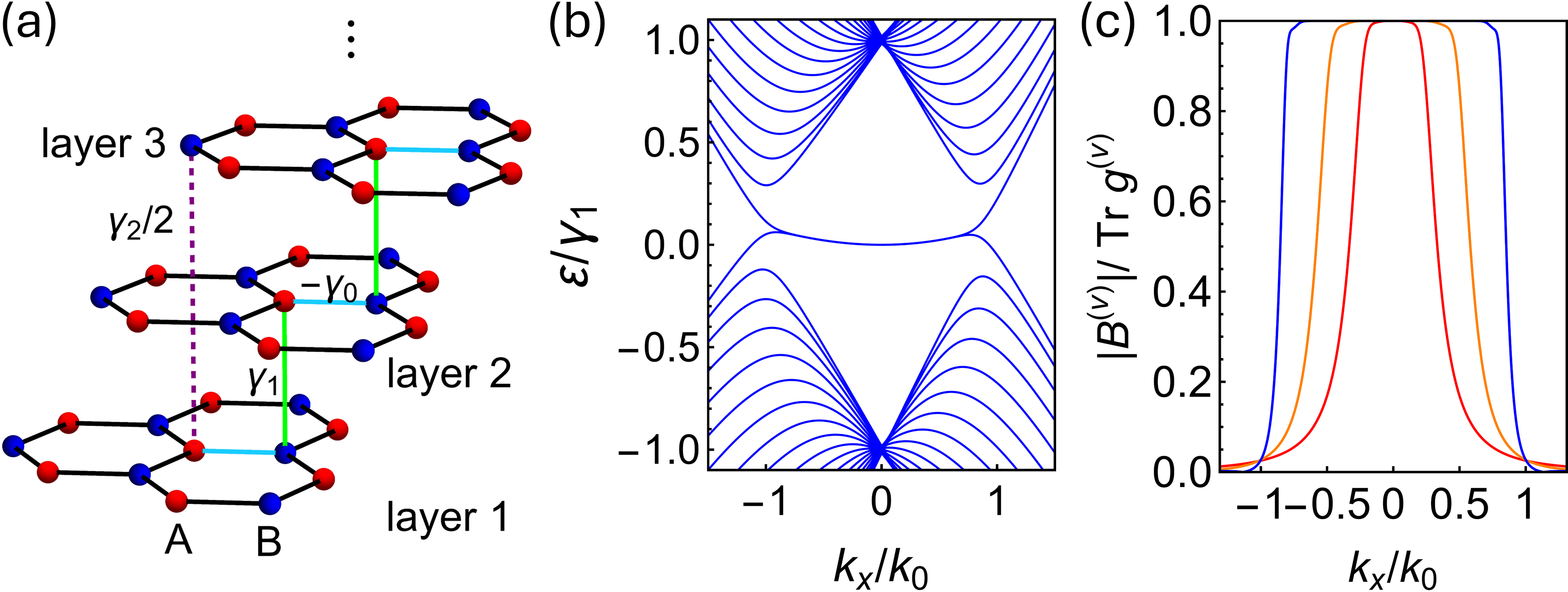
Figure 1: (a) Lattice structure of RG (3 layers are shown). Red and blue spheres represent the A/B sublattices. The light blue and green bonds (representing the hopping integrals $-\gamma_{0}$, $\gamma_{1}$) form the staircase unit cell of multilayer RG. The purple dashed bond indicates the next-nearest interlayer coupling $\gamma_{2}/2$ (additional coupling parameters can be found in supplementary Sec. S1). (b) Band structure of 20-layer RG without displacement field at valley $K$, with two drumhead-like surface bands at low energies. (c) Local inequality between quantum metric and Berry curvature is saturated in RG surface bands ($\text{Tr}g^{(v)}=|B^{(v)}|$) at the center of the drumhead region. They are calculated from 3 (red), 6 (orange) and 20 (blue)-layer RG continuum models with $\gamma_{0},\gamma_{1}$ couplings and surface potential $m=0.01\gamma_{1}$.

Quantum geometry of the surface states of $N$-layer RG in the $N\rightarrow\infty$ limit.—We begin with an analysis of the QGT [67, 68] of RG surface bands and discuss its two fundamental properties: it is nonzero at the center and peaked at the rim of the drumhead region. Both properties result from the momentum-dependent decay of the evanescent surface states. Therefore, they are generic for the drumhead-like surface bands of other NLS as well.

The drumhead region of RG surface bands at each valley has a radius $k_{0}=\gamma_{1}/v_{f}$ (we set $\hbar=1$), with $\gamma_{1}$ the nearest-neighbor interlayer coupling constant [see Fig. 1(a,b)] and $v_{f}$ the Fermi velocity of single-layer graphene. This is quite a small area (0.3%) compared to the surface BZ of RG, making it tunable by gate voltage in a nearby electrode, similar to MATBG. The radius $k_{0}$ sets a natural momentum scale for RG surface bands, beyond which the surface states become bulk states. This implies that the inverse of the decay length of the surface states, $\kappa$, which is complex in general, varies with the in-plane momentum k [69, 13]. To analyze the QGT, we solve the surface states analytically from the bulk Hamiltonian subject to an open boundary condition [13] (see supplementary Sec. S2.1), similar to solving the graphene zigzag edge modes [70, 71, 72, 73]. We simplify the problem by taking the RG model with $\gamma_{0},\gamma_{1}$ couplings only and focus on the limit of a large number of layers, $N\rightarrow\infty$. In the next section, we explain why QGT in this limit is the same at the center of the drumhead region as in RG with small $N$. For $N\rightarrow\infty$, the two normalized surface states at the valley $K$ are (valley $K^{\prime}$ is related to $K$ by the assumed time-reversal symmetry)

$$\begin{split}&\psi^{(1)}_{\textbf{k}}(z)=\frac{\sqrt{1-k^{2}}}{k}e^{\kappa(\textbf{k})z}\begin{pmatrix}1\\ 0\end{pmatrix},\\ &\psi^{(2)}_{\textbf{k}}(z)=\frac{\sqrt{1-k^{2}}}{k}e^{\kappa(\textbf{k})^{*}(N+1-z)}\begin{pmatrix}0\\ 1\end{pmatrix},\end{split}$$ (1)

where $z$ is the layer index running from 1 to $N$ ($\rightarrow\infty$), $k=|\textbf{k}|$, $\kappa(\textbf{k})=\ln[-(k_{x}+ik_{y})]$ , and the two-component spinor is for A/B sublattice. We have chosen $k_{0}$ as the unit of momentum, so k is dimensionless. The two surface states are degenerate in the entire region $k<1$, with energy $\varepsilon=0$. Therefore, any linear combination of them is also an eigenstate. However, they remain in the form of Eq. (1) if the degeneracy is lifted by a small potential $m$ with opposite signs on the two surfaces.

Using the definition of QGT $\mathcal{B}^{(i)}_{\mu\nu}(\textbf{k})=\text{Tr}\{P^{(i)}_{\textbf{k}}\partial_{\mu}P^{(i)}_{\textbf{k}}\partial_{\nu}P^{(i)}_{\textbf{k}}\}$ ($\mu$, $\nu$ denote $x$, $y$ and $\partial_{\mu}\equiv\partial/\partial k_{\mu}$), where $P^{(i)}_{\textbf{k}}=|\psi^{(i)}_{\textbf{k}}\rangle\langle\psi^{(i)}_{\textbf{k}}|$ is the projection to band $i$ ($=1,2$), QGT of the two bands can be written in terms of the gradient $\nabla\kappa(\textbf{k})$ and moments of the function $e^{(\kappa+\kappa^{*})z}$ (see supplementary Sec. S2.1 for details), giving

$$\mathcal{B}^{(1,2)}_{\mu\nu}(\textbf{k})=\frac{1}{(1-k^{2})^{2}}\begin{pmatrix}1&\pm i\\ \mp i&1\end{pmatrix}$$ (2)

where the upper (lower) sign is for $\mathcal{B}^{(1)}$ ($\mathcal{B}^{(2)}$). Since $\mathcal{B}^{(i)}_{\mu\nu}\equiv g^{(i)}_{\mu\nu}+\frac{i}{2}B^{(i)}_{\mu\nu}$, it tells us that the two surface bands have equal QM ($g^{(i)}_{\mu\nu}$) and opposite Berry curvature ($B^{(i)}_{\mu\nu}$). The local inequality between the QM and Berry curvature, $\text{Tr}\,g^{(i)}(\textbf{k})\geq|B^{(i)}(\textbf{k})|$ is saturated [65, 75, 76], i.e, the inequality is an equality here. This makes the two bands analogous to a pair of LLLs with opposite magnetic fields. The differences with LLLs are: the QGT is k-dependent, and the total Berry phase in the drumhead region $k<1$ diverges as $N\rightarrow\infty$ [77].

Importantly, the two states in Eq. (1) are localized at opposite surfaces and composed of sublattice A or B only, meaning that they are atomically decoupled. Then the interband (band-resolved) QGT between them vanishes, $\mathcal{B}^{(12)}_{\mu\nu}=0$ where $\mathcal{B}^{(12)}_{\mu\nu}\equiv-\langle\partial_{\mu}\psi^{(1)}_{\textbf{k}}|\psi^{(2)}_{\textbf{k}}\rangle\langle\psi^{(2)}_{\textbf{k}}|\partial_{\nu}\psi^{(1)}_{\textbf{k}}\rangle$. As a result, the total nonabelian QGT of the two bands,

$$\mathcal{B}^{(\text{tot})}_{\mu\nu}\equiv\mathcal{B}^{(1)}_{\mu\nu}+\mathcal{B}^{(2)}_{\mu\nu}+2\mathcal{B}^{(12)}_{\mu\nu}=\mathcal{B}^{(1)}_{\mu\nu}+\mathcal{B}^{(2)}_{\mu\nu}$$ (3)

is a sum of the two intra-band contributions only, which have nonzero QM. This simple result shows that a two-band model constructed from two Wannier orbitals cannot describe the quantum geometry of the two surface bands in the drumhead region, because the total quantum metric of a two-band model is always zero. For instance, the two-band effective Hamiltonian of RG derived by projecting the continuum model to the two surface orbitals [78, 79, 80, 77] is unable to capture the out-of-plane decay properties of the states, and thus it has zero QM at the center of the drumhead region [81].

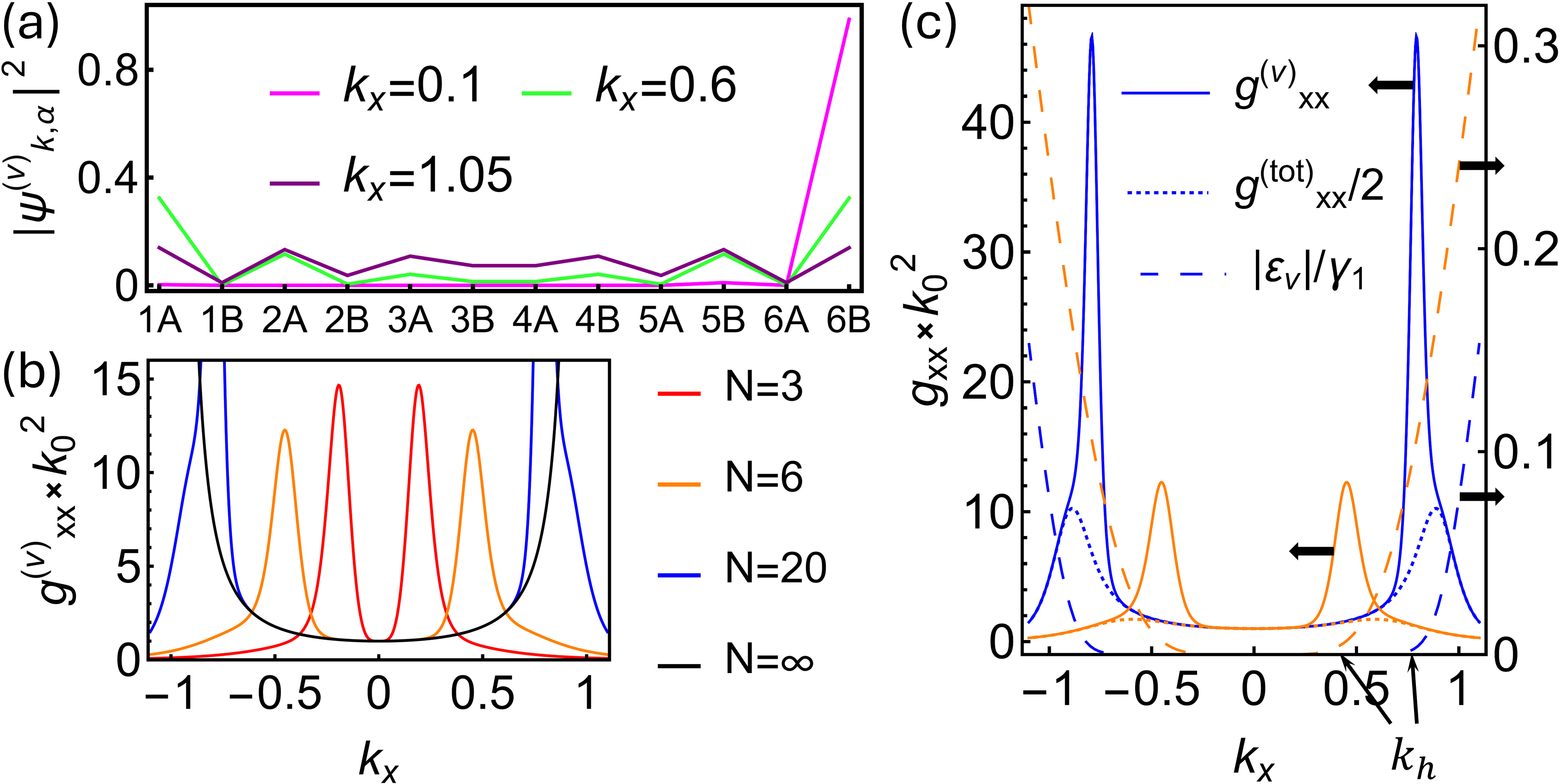
Figure 2: RG model with $\gamma_{0}$, $\gamma_{1}$ couplings and surface potential $m=0.01\gamma_{1}$ (to open a small band gap). (a) State profile $|\psi^{(v)}_{\textbf{k},\alpha}|^{2}$ for various $k_{x}$ (in the units of $k_{0}$), and $k_{y}=0$ in the valence band of 6-layer RG at valley $K$. (b) QM of the valence surface band for various $N$-layer RG. The black curve corresponds to the result for $N\rightarrow\infty$, $g^{(v)}_{xx}(\textbf{k})=1/(1-k^{2})^{2}$. (c) The valence band QM, $g^{(v)}_{xx}$, vs. half of the total nonabelian QM, $g^{(\text{tot})}_{xx}/2$, of the two surface bands, and the dispersion $|\varepsilon_{v}|$ for 6 (orange) and 20 (blue) -layer RG.

Surface hybridization effect.—QGT of the RG surface bands has a second interesting property; that is, it is sharply peaked at the rim of the drumhead region, as demonstrated below using RG with a small number of layers. When $N$ is small, besides $k_{0}$, another momentum scale, $k_{h}$ becomes important. Since the decay length of the surface states, $\lambda\equiv 1/|\kappa|$ is k-dependent, at some critical value $k_{h}$, it gets comparable with the thickness, $\lambda(k_{h})\sim N$. Momentum $k_{h}$ characterizes where the two surfaces start to hybridize, and it can be estimated as $k_{h}=k_{0}e^{-\eta/N}$, with $\eta$ a constant of the order of unity. In the band structure, this hybridization splits the two surface bands (we call the new bands valence and conduction bands); therefore, for small $N$, the rim of the drumhead region is determined by $k_{h}$ rather than $k_{0}$. As $N\rightarrow\infty$, $k_{h}/k_{0}\rightarrow 1$.

In Fig. 2(a), we plot the probability density of the 12 orbitals for the valence band surface state of the representative 6-layer RG at different momenta. To avoid degeneracies between the two bands, we always add a small surface potential $\pm m$ to open a band gap (however, this is unnecessary for computing the nonabelian $\mathcal{B}^{(\text{tot})}$). It shows that at $k\in(k_{h},k_{0})$ (for $N=6$, $k_{h}\sim 0.3k_{0}$), the states are still surface states but behave as “bulk-like” due to the hybridization (green curve); at $k>k_{0}$, they become real bulk states with $|\kappa|=0$.

Figure 2(b) shows the valence band QM numerically calculated from the continuum model for various $N$-layer RG in the drumhead region. In the center, they always coincide with the analytical result in the $N\rightarrow\infty$ limit, Eq. (2). The reason is that whenever $k<k_{h}$, in the absence of surface hybridization, the surface states for small $N$ are the same as those in the $N\rightarrow\infty$ limit. In addition, we observe sharp peaks of QM for the surface band. We ascribe such behavior to surface hybridization and explain it using Fig. 2(c).

In Fig. 2(c), we first contrast the valence band QM $g^{(v)}$ with the dispersion $|\varepsilon_{v}|$, finding that the peaks of $g^{(v)}$ are exactly located at $k_{h}$ where the two bands split. Intuitively, this is because at $k<k_{h}$ the surface state $\psi^{(v)}_{\textbf{k}}$ as a function of k varies with the layer index $z$ only (Eq. (1)), while it also varies between the A/B sublattices at $k\in(k_{h},k_{0})$ due to the surface hybridization. To prove this interrelation, we compare $g^{(v)}$ with half of the non-abelian QM of the two bands, $g^{(\text{tot})}/2$. The difference between the two (solid and dotted) curves gives the interband QM component $-g^{(vc)}$ ($g^{(vc)}\equiv\text{Re}\mathcal{B}^{(vc)}$), which is a positive semidefinite quantity. Since $g^{(vc)}$ vanishes in the $N\rightarrow\infty$ limit (i.e. $g^{(12)}=0$ from Eq. (1)), it contains information about surface hybridization. We find that the peak of $g^{(v)}$ is mainly contributed by that of $-g^{(vc)}$ rather than $g^{(\text{tot})}/2$. However, $g^{(\text{tot})}$ exhibits a small peak, resulting from the small bandgap between the surface and bulk bands. Since this bandgap decreases with increasing $N$ [82, 83, 84], the peak of $g^{(\text{tot})}$ is negligible for $N=6$ but pronounced for $N=20$.

We have thus established the quantum geometric properties of the RG surface states using the simplified model with only $\gamma_{0}$ and $\gamma_{1}$ couplings. When the long-range couplings are included, these qualitative results remain valid (see supplementary Sec. S2.3) except for RG with only a few layers. We elucidate this below as we discuss the superconducting state. Before moving on, we comment on how these properties are related to the FCI states. Fig. 1(c) shows $|B^{(v)}|/\text{Tr}g^{(v)}$ for the valence surface band of RG, which is perfectly saturated at $k<k_{h}$, as dictated by Eq. (2). Therefore, the proposed geometric stability hypothesis [64, 65, 66] can in principle be responsible for the observed FCI phases [52, 53]. Since the factor $1/(1-k^{2})^{2}$ in Eq. (2) varies slowly at the center of the drumhead region, the moiré potential can keep the region with the most uniform QGT as the active band by zone folding. However, the specific role of superlattice potential at the edge of the moiré BZ is worth further studies [63, 53].

Superconducting state and surface polarization.—We use the superconducting phase of RTG labeled by SC1 in Ref. [31] as a starting point to understand the RG surface superconductivity. In RTG, the next-nearest interlayer hopping $\gamma_{2}/2$ directly couples the two surfaces [Fig. 1(a)], changing the previous discussions about $k_{h}$ and surface hybridization. It leads to an overall separation of $\gamma_{2}$ between the two bands [Fig. 3(a)]. In this case, the largest DOS is at the Van Hove singularity (VHS), near where the superconducting phases were found.

We consider an onsite attractive interaction model for RG, $\hat{H}_{I}=-U\sum_{i}\hat{n}_{i\uparrow}\hat{n}_{i\downarrow}$ ($U>0$), where the effective attractive interaction could arise from different types of physical mechanisms [85, 86, 87, 50]. Here $\hat{n}_{i\sigma}$ is the density operator for spin $\sigma$ at carbon site $i$. We assume an inter-valley pairing superconducting state and restrict to the $s$-wave pairing channel; the possibilities of other pairing symmetries [85, 86, 51] are beyond the scope of this work. For band structure calculations, we adopt the parameter system suggested by Refs. [77, 88, 89] for RTG and use the specific parameters given in Ref. [89] (see supplementary Sec. S1). We also give an analysis of the phase diagram of SC1 based on the onsite attractive interaction model in supplemental Sec. S4.1.

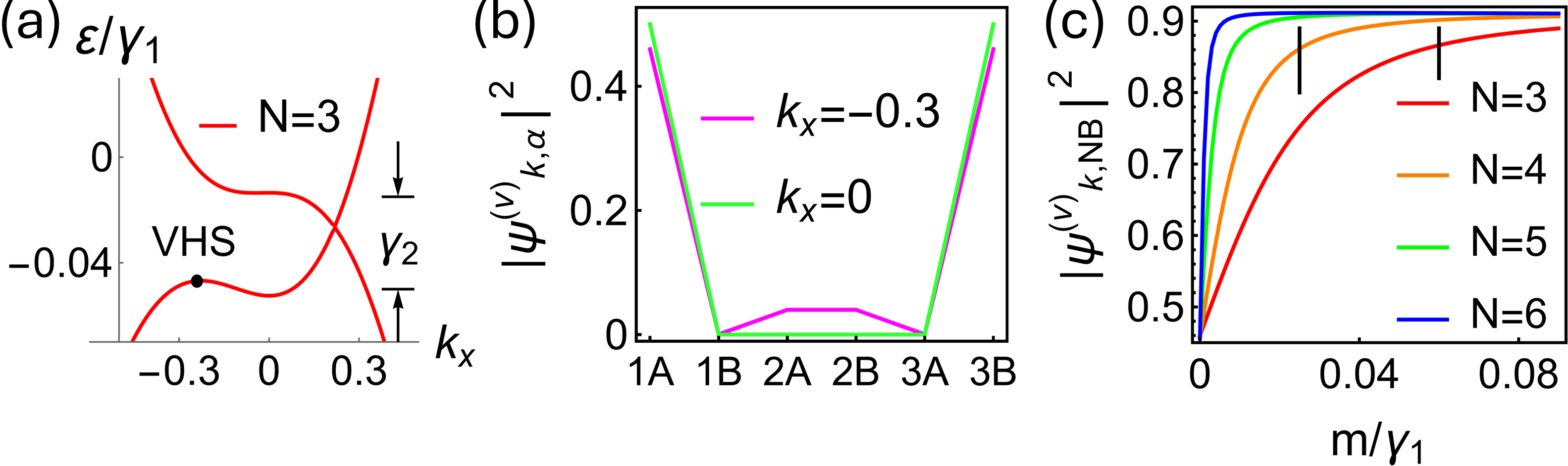
Figure 3: (a) Surface band dispersion near $K$ for RTG at $m=0$. (b) Probability density $|\psi^{(v)}_{\textbf{k},\alpha}|^{2}$ of RTG valence surface state at $\textbf{k}=(-0.3,0)$ (near the VHS), and $\textbf{k}=(0,0)$ at $m=0$. (c) $|\psi^{(v)}_{\textbf{k},N\text{B}}|^{2}$ of surface orbital $N$B at $\textbf{k}=(-0.3,0)$ as a function of the surface potential $m$, for various few-layer RG. The vertical bars indicate the value $m_{s}$ where the density polarization saturates for trilayer and tetralayer.

We now explain the surface polarization effect, which can be important for understanding the metal-superconductor transition in RTG. The displacement field has two different effects: the first is to flatten the band and enhance the DOS peak, while the second is to polarize the electron densities to only one surface orbital [90]. At zero displacement field, the $\gamma_{2}$ coupling hybridizes the two surface orbitals 1A and 3B at layers 1 and 3 in a band, each with 45% probability density (less than 50% due to the nonzero decay length) near the VHS, as shown in Fig. 3(b). As $m$ increases, one of the two orbitals becomes fully polarized (90%) and the polarization saturates around $m_{s}=0.06\gamma_{1}$ (23 meV). This effect exists extensively for few-layer RG but is most noticeable in RTG. As the thickness increases, $m_{s}$ decreases rapidly [Fig. 3(c)] and becomes infinitesimal for thick RG slabs. Once $m$ is above $m_{s}$, the earlier picture of the k-dependence of surface hybridization is restored, and $k_{h}$ becomes well-defined again.

To see how the surface polarization affects the superconducting state, we solve the zero-temperature gap equation $\Delta_{\alpha}\equiv-U\langle c_{\textbf{R}\alpha\downarrow}c_{\textbf{R}\alpha\uparrow}\rangle$ of each orbital $\alpha$ for $N$-layer RG (see supplementary Sec. S3.1), with $c_{\textbf{R}\alpha\sigma}$ the annihilation operator for unit cell R and $\alpha=$1A, 1B, …, $N$B running over the $2N$ orbitals in a unit cell. In RG, since the interaction $U$ is weak and the DOS is concentrated at the two surface orbitals, the only non-negligible order parameters are $\Delta_{1\text{A}}$ and $\Delta_{N\text{B}}$. Then the order parameter in the band basis, $\Delta_{v,\textbf{k}}\equiv\langle\psi^{(v)}_{\textbf{k}}|\hat{\Delta}|\psi^{(v)}_{\textbf{k}}\rangle$, with $\hat{\Delta}=\text{diag}(\Delta_{\alpha})$ the pairing matrix in the orbital basis, is

$$\Delta_{v,\textbf{k}}=|\psi^{(v)}_{\textbf{k},1\text{A}}|^{2}\Delta_{1\text{A}}+|\psi^{(v)}_{\textbf{k},N\text{B}}|^{2}\Delta_{N\text{B}}.$$ (4)

We have assumed that the $N$-layer RG is doped to the valence band and $\Delta_{1\text{A}},\Delta_{N\text{B}}$ are smaller than the relevant band gaps. The linear combination form of Eq. (4) implies that the set of two order parameters $\{\Delta_{1\text{A}},\Delta_{N\text{B}}\}$ is more informative than $\Delta_{v,\textbf{k}}$, which is examplified by the surface polarization here. As the superconducting transition is determined by the larger one of $\Delta_{1\text{A}}$ and $\Delta_{N\text{B}}$, one can compare the two cases of different surface potentials, $m=0$ and $m=m_{s}$, and find that the coupling strength for the order parameter $\Delta_{N\text{B}}$ is doubled in the case $m=m_{s}$ due to the polarization effect (see supplementary Sec. S4.2 for further details). This factor of 2 is crucial since SC1 is in the weak coupling limit; in addition, $m_{s}$ of RTG (23 meV) is likely to be close to the onset surface potential of SC1 that corresponds to its endpoint at $10^{12}$ cm^-2 hole density as observed in Ref. [31]. Therefore, surface polarization plays an important role in the superconducting transition to SC1 as the displacement field increases.

RG as a flat-band superconductor and comparison with MATBG.—It is theoretically inspiring to formally treat RG as a flat-band superconductor and compare it with another example—MATBG. For this purpose, we consider a fictitious superconducting state in a large-$N$-layer RG doped to the valence band and study the distribution of its superfluid weight in momentum space.

The calculation of superfluid stiffness in RG dates back to Kopnin [27], who found a finite supercurrent from the rim of the drumhead region despite the surface bands being dispersionless at the center. However, the quantum geometric properties [75, 91] have not been characterized. Using the grand potential formalism [75, 92] and the single-valence-band projection scheme [93], the zero-temperature superfluid weight has the integral form $D_{s,\mu\nu}=2\sum_{\textbf{k}\in\Lambda_{K}}[f^{\text{conv}}_{\mu\nu}(\textbf{k})+f^{\text{geo}}_{\mu\nu}(\textbf{k})]$, with the factor 2 for valley degeneracy and integrands

$$f^{\text{conv}}_{\mu\nu}(\textbf{k})=-\bigg{(}\frac{\xi_{v,\textbf{k}}}{E_{v,\textbf{k}}}+1\bigg{)}\partial_{\mu}\partial_{\nu}\xi_{v,\textbf{k}},$$ (5)

$$f^{\text{geo}}_{\mu\nu}(\textbf{k})= \frac{1}{E_{v,\textbf{k}}}\text{Tr}\{\partial_{\mu}P^{(v)}_{\textbf{k}}\hat{\Delta}\partial_{\nu}P^{(v)}_{\textbf{k}}\hat{\Delta}-\partial_{\mu}\partial_{\nu}P^{(v)}_{\textbf{k}}\hat{\Delta}P^{(v)}_{\textbf{k}}\hat{\Delta}\}.$$ (6)

Here $\hat{\Delta}=\text{diag}(0,...,0,\Delta_{N\text{B}})$, with $\Delta_{1\text{A}}=0$ due to the polarization, $\xi_{v,\textbf{k}}=\varepsilon_{v,\textbf{k}}-\mu$ is the dispersion, with $\mu$ the chemical potential, and $E_{v,\textbf{k}}$ is the Bogoliubov quasi-particle energy.

In Fig. 4(a), we plot these two integrands calculated from the continuum model of 20-layer RG with only $\gamma_{0},\gamma_{1}$ couplings. To amplify the geometric contribution, we use a relatively large order parameter $\Delta_{20\text{B}}=0.02\gamma_{1}$ . We find that both integrands peak at the rim of the drumhead region, in stark contrast with the order parameter in the band basis (dashed curve). The latter approaches a bell-shape function $\Delta_{v,\textbf{k}}=\Delta_{N\text{B}}(1-k^{2})$ as $N\rightarrow\infty$ [26], with nodes at the rim region resulting from the decrease of the weight of orbital $N$B as the surface states transit to bulk states.

These features make RG resemble the heavy-fermion compounds [95, 96, 97, 98], particularly the topological heavy-fermion (THF) model of MATBG that was established recently [99, 100]. In the THF model, the low-energy bands of MATBG are described by $f$ and $c$ orbitals, which hybridize near the $\Gamma_{M}$ point only [see Fig. 4(b)]. Since the superconducting order parameters on these $c$ orbitals are negligible due to their low composition in the quasi-flat bands, the order parameter of MATBG in the band basis would be large and uniform at the k-points far from $\Gamma_{M}$, but diminishes near $\Gamma_{M}$.

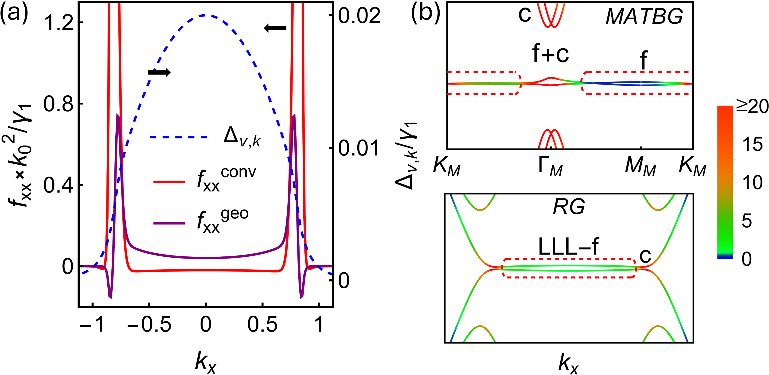
Figure 4: (a) Superfluid weight integrands vs order parameter $\Delta_{v,\textbf{k}}$ for 20-layer RG doped to the valence band, using $\Delta_{20\text{B}}=0.02\gamma_{1}$, $m=-\mu=0.01\gamma_{1}$. (b) Schematic band structure of MATBG and RG with their $f$-electrons enclosed in dashed contours and the scaled QM of bands indicated by colors . In MATBG, $f$-electrons have zero QGT; the hybridization with $c$-electrons and the mixing between the two $f$-electrons give concentrated QM near $\Gamma_{M}$ and $K_{M}$, respectively. In RG, “$f$-electrons” have the quantum geometry of the LLL. In both cases, $f$-electrons lead to the superconducting gap while $c$-electrons lead to superfluidity, but the LLL-like “$f$-electrons” in RG also contribute to superfluidity through quantum geometry.

The superfluid weight for MATBG based on quantum geometry has been discussed in several works [101, 102, 103, 5], but here, we address some features that have not been captured before. The QM of the quasi-flat bands calculated from the continuum model can be seen from Fig. 4(b) (also see Ref. [104]), showing that it vanishes in the moiré BZ except near $\Gamma_{M}$ due to the hybridization (i.e., topology [103, 105]) and near $K_{M}$, $K^{\prime}_{M}$ due to band crossings. However, the superconducting gap in MATBG is about 2 meV [106], which is larger than the separation between the two bands near $K_{M}$, $K^{\prime}_{M}$, and in particular, the two bands near $K_{M}$, $K^{\prime}_{M}$ can be described by a two-orbital model, according to the THF model. Then the interband effect between bands in the interaction scale [102, 107] would completely cancel the geometric superfluid weight from $K_{M}$, $K^{\prime}_{M}$. Thus, we conclude that only the k-points near $\Gamma_{M}$ contribute to the superfluidity of MATBG .

In RG, the momentum scale $k_{h}$ roughly classifies the electrons as dispersionless, strongly localized surface states (for $k<k_{h}$) and dispersive, “bulk-like” surface states (for $k_{h}<k<k_{0}$), which mimic the $f$ and $c$ orbitals in a heavy-fermion model, respectively [Fig. 4(b)] . Compared to MATBG, the heavy fermion picture for RG is unusual in the sense that the Cooper pairs formed by the “$f$-electrons” can transport supercurrent, as shown by the purple curve in Fig. 4(a). This is manifested in $f^{\text{geo}}_{\mu\nu}$ in Eq. (6) which can be understood as the QM “projected” to the surface orbital through the operator $\hat{\Delta}$ (for $\hat{\Delta}$ proportional to identity matrix, $f^{\text{geo}}_{\mu\nu}$ is proportional to QM). Even when the valence surface band is a single band where only one orbital has nonzero superconducting order, the k-dependence of the density of orbital $N$B in the band leads to the nonzero $f^{\text{geo}}_{\mu\nu}$ at the center of the drumhead region.

Discussion.—We have studied the quantum geometric properties of RG surface bands that arise from the evanescent nature of the surface states, the effect of surface hybridization, and how the surface polarization by the displacement field boosts the superconducting transition in few-layer RG, e.g., RTG. With a quantum metric that is nonzero at the center and peaked at the rim of the drumhead region, multilayer RG qualitatively fits in an intriguing heavy-fermion picture, which is different from MATBG, as the quantum geometry of the two surface bands cannot be described by a two-orbital model. Although superconductivity in thick RG samples has not been found [37], these quantum geometric properties may be detected by susceptibilities of other correlated states. Different from some earlier works [59, 61], we show that even before forming the anomalous Hall crystal, the noninteracting surface states of RG have similar quantum geometry to the LLL. This analogy constrains the low-energy models constructed for its correlated phases and sheds light on future studies for RG and fractional topological phases.

Supplementary material for “Quantum geometry of the surface states of rhombohedral graphite and its effects on the surface superconductivity”

I S1: Non-interacting Hamiltonian of rhombohedral graphite and rhombohedral multilayer graphene

The Bravais lattice vectors for a single-layer graphene are chosen as $\textbf{a}_{1}=(1,0)a_{0}$, $\textbf{a}_{2}=(\frac{1}{2},\frac{\sqrt{3}}{2})a_{0}$, and the three nearest-neighbor hopping vectors from sublattice A to B are $\bm{\delta}_{1}=(0,\frac{\sqrt{3}}{3})a_{0}$, $\bm{\delta}_{2}=(-\frac{1}{2},-\frac{\sqrt{3}}{6})a_{0}$, $\bm{\delta}_{3}=(\frac{1}{2},-\frac{\sqrt{3}}{6})a_{0}$ [Fig. S1(a)]. Atom A at $(0,0)$ and B at $\bm{\delta}_{1}$ are grouped as a unit cell. Dirac points of the two valleys, $K,K^{\prime}$, are chosen as $K=\frac{2\pi}{a_{0}}(\frac{2}{3},0)$, $K^{\prime}=\frac{2\pi}{a_{0}}(-\frac{2}{3},0)$. For multilayer RG, the $(n+1)$-th layer can be viewed as the $n$th layer shifted by vector $\bm{\delta}_{1}$ in the basal plane, therefore, the unit cell is chosen as the staircase structure consisting of horizontal ($\bm{\delta}_{1}$) and vertical ($c\hat{z}$) bonds, as shown in Fig. S1(b). The tight-binding Hamiltonian in real space including all hoppings reads

$$\begin{split}\hat{H}=&-\gamma_{0}\sum_{\langle i,j\rangle\sim\gamma_{0}}\sum_{\sigma}c_{i\sigma}^{\dagger}c_{j\sigma}+\gamma_{1}\sum_{\langle i,j\rangle\sim\gamma_{1}}\sum_{\sigma}c_{i\sigma}^{\dagger}c_{j\sigma}+\frac{\gamma_{2}}{2}\sum_{\langle i,j\rangle\sim\gamma_{2}}\sum_{\sigma}c_{i\sigma}^{\dagger}c_{j\sigma}\\ &-\gamma_{3}\sum_{\langle i,j\rangle\sim\gamma_{3}}\sum_{\sigma}c_{i\sigma}^{\dagger}c_{j\sigma}-\gamma_{4}\sum_{\langle i,j\rangle\sim\gamma_{4}}\sum_{\sigma}c_{i\sigma}^{\dagger}c_{j\sigma},\end{split}$$ (S1)

where $i,j$ generically label all the carbon sites and $\sigma=\uparrow$ or $\downarrow$ labels the spin. Symbol $\langle i,j\rangle\sim\gamma_{s}\,(s=0,1,...,4)$ refers to the pairs of sites $i,j$ that are linked by the hopping $\gamma_{s}$. The sum includes both the $\{i,j\}$ and the $\{j,i\}$ terms of the pair to make the Hamiltonian hermitian. The site label $i$ can also be replaced with the tuple $\textbf{R}\alpha$, where the in-plane vector R labels the unit cell, and $\alpha$ runs over the $2N$ orbital indices in a unit cell, 1A, 1B, …, $N$A, $N$B. We define R to be the position of atom A in the 1st layer (atom 1A).

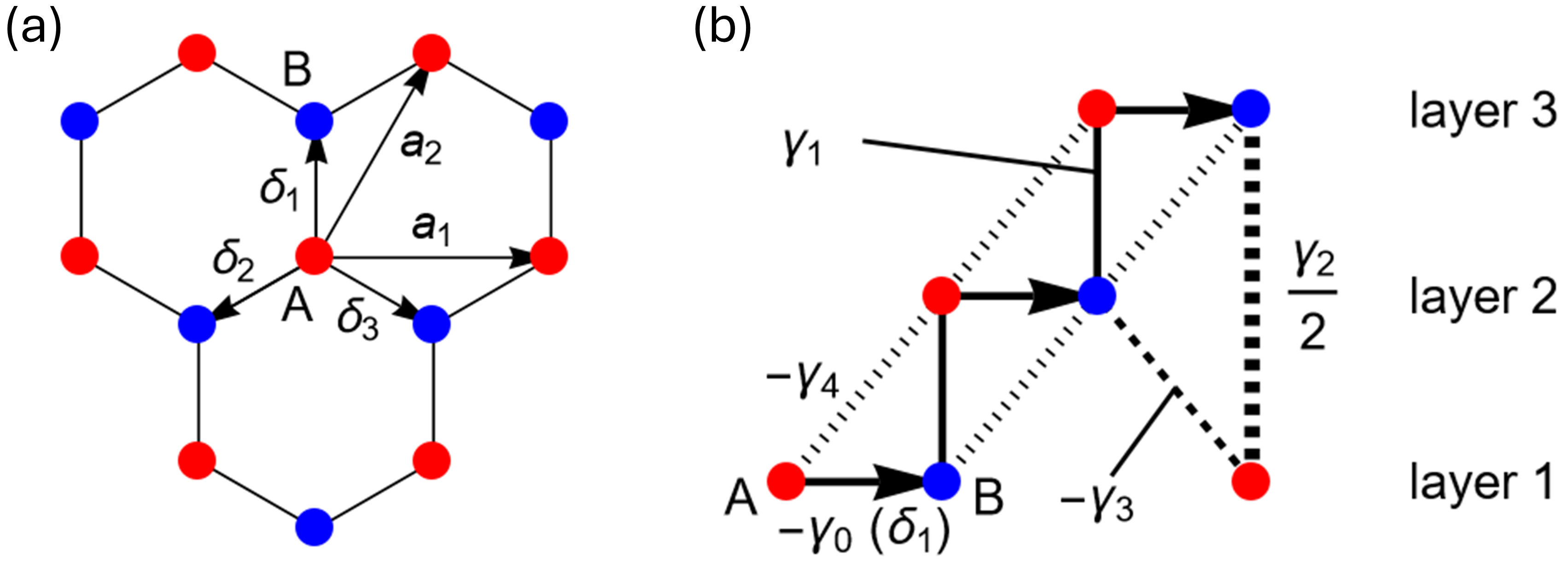
Figure S1: Summary of conventions for the RG multilayers. (a) $\textbf{a}_{1},\textbf{a}_{2}$ are the Bravais lattice vectors and $\bm{\delta}_{1},\bm{\delta}_{2},\bm{\delta}_{3}$ are the three nearest-neighbor hopping vectors. (b) Side view of RG multilayers from $\textbf{a}_{1}$ direction with hopping integrals $-\gamma_{0}$, $\gamma_{1}$, $\gamma_{2}/2$, $-\gamma_{3}$ and $-\gamma_{4}$.

To obtain the continuum model Hamiltonian, we perform the Fourier transformation of field operators with a local gauge choice, $c_{\textbf{k}\alpha\sigma}\equiv\frac{1}{\sqrt{N_{c}}}\sum_{\textbf{k}}e^{-i\textbf{k}\cdot(\textbf{R}+\textbf{x}_{\alpha})}c_{\textbf{R}\alpha\sigma}$ ($\alpha=$1A, 1B,…, $N$A, $N$B), where $\textbf{x}_{n\text{A}}=(n-1)\bm{\delta}_{1}$, $\textbf{x}_{n\text{B}}=n\bm{\delta}_{1}$ ($n$ is the layer index) are the positions of the orbitals in the unit cell measured from 1A. Under these conventions and gauge choices, the intra-layer hopping term gives the usual Dirac effective Hamiltonian

$$\hat{H}^{(\gamma_{0})}=\sum_{\textbf{k},\sigma}\sum_{n=1}^{N}\psi_{n\textbf{k}\sigma}^{\dagger}h_{K(K^{\prime})}(\textbf{k})\psi_{n\textbf{k}\sigma},$$ (S2)

where $h_{K(K^{\prime})}(\textbf{k})=\frac{\sqrt{3}}{2}\gamma_{0}a_{0}(\xi\sigma_{x}k_{x}+\sigma_{y}k_{y})$, with $\xi=\pm$ for valley $K$ and $K^{\prime}$, respectively, and k is the in-plane momentum measured from $K$ or $K^{\prime}$. The two-component spinor $\psi_{n\textbf{k}\sigma}\equiv(c_{\textbf{k},n\text{A},\sigma},c_{\textbf{k},n\text{B},\sigma})^{T}$.

Throughout the paper, we assume valley degeneracy. The Hamiltonian at valley $K^{\prime}$ is related to that at $K$ by time-reversal symmetry (TRS). The Hamiltonian terms associated with $\gamma_{1}-\gamma_{4}$ couplings near $K$ are

$$\hat{H}^{(\gamma_{1})}=\sum_{\textbf{k},\sigma}\sum_{n=1}^{N-1}\psi_{n+1,\textbf{k}\sigma}^{\dagger}(\gamma_{1}\sigma_{+})\psi_{n\textbf{k}\sigma}+h.c.,$$ (S3)

$$\hat{H}^{(\gamma_{2})}=\sum_{\textbf{k},\sigma}\sum_{n=1}^{N-2}\psi_{n+2,\textbf{k}\sigma}^{\dagger}(\frac{\gamma_{2}}{2}\sigma_{-})\psi_{n\textbf{k}\sigma}+h.c.,$$ (S4)

$$\hat{H}^{(\gamma_{3})}=\sum_{\textbf{k},\sigma}\sum_{n=1}^{N-1}\psi_{n+1,\textbf{k}\sigma}^{\dagger}\big{[}\frac{\sqrt{3}}{2}\gamma_{3}a_{0}(k_{x}-ik_{y})\sigma_{-}\big{]}\psi_{n\textbf{k}\sigma}+h.c.,$$ (S5)

$$\hat{H}^{(\gamma_{4})}=\sum_{\textbf{k},\sigma}\sum_{n=1}^{N-1}\psi_{n+1,\textbf{k}\sigma}^{\dagger}\big{[}\frac{\sqrt{3}}{2}\gamma_{4}a_{0}(k_{x}+ik_{y})\sigma_{0}\big{]}\psi_{n\textbf{k}\sigma}+h.c.$$ (S6)

where $\sigma_{\pm}=\sigma_{x}\pm i\sigma_{y}$. Besides these terms, there are also onsite potential terms, including the surface potential parameter, etc.

Parameters fit for RTG are taken from Ref. [89]: $\gamma_{0}=3.1$ eV, $\gamma_{1}=0.38$ eV, $\gamma_{2}=-0.015$ eV, $\gamma_{3}=-0.29$ eV, $\gamma_{4}=-0.141$ eV, $\Delta_{2}=-0.0023$ eV and $\delta=-0.0105$ eV. We use the symbol $m$ instead of $\Delta_{1}$ to denote the surface potential; $\Delta_{2}$ and $\delta$ are potential parameters describing the asymmetry between A and B sublattices on the surfaces and the nonuniform potential drop along $z$ direction (see Eq. (S8)).

For RG with more than three layers, we use the same parameters $\gamma_{0}-\gamma_{4}$ as those for RTG, though some of them are sensitive to the number of layers and depend on the sample conditions. Without knowing the variation of potential with layers, we make a metallic assumption that the potential only drops between the surfaces and adjacent layers, therefore, the potentials of different layers are $m$, 0, 0, …, $-m$.

The Fermi velocity of single-layer graphene is $v_{f}=\frac{\sqrt{3}}{2}\gamma_{0}a_{0}$ and we define $v_{3}=\frac{\sqrt{3}}{2}\gamma_{3}a_{0}$, $v_{4}=\frac{\sqrt{3}}{2}\gamma_{4}a_{0}$. Choosing $\gamma_{1}$ and $k_{0}=\gamma_{1}/v_{f}$ as the units of energy and momentum, respectively, the Hamiltonian can be written in terms of dimensionless parameters $\widetilde{\gamma}_{2}=\gamma_{2}/\gamma_{1}\approx-0.039$, $\widetilde{m}=m/\gamma_{1}$, $\widetilde{\Delta}_{2}=\Delta_{2}/\gamma_{1}=-0.006$, $\widetilde{\delta}=\delta/\gamma_{1}=-0.028$ and

$$\widetilde{v}_{3}=\frac{v_{3}}{v_{f}}=\frac{\gamma_{3}}{\gamma_{0}}\approx-0.094,\,\,\,\,\,\,\widetilde{v}_{4}=\frac{v_{4}}{v_{f}}=\frac{\gamma_{4}}{\gamma_{0}}\approx-0.045.$$ (S7)

For instance, the dimensionless $6\times 6$ continuum model Hamiltonian for RTG including the onsite potentials, reads

$$H^{\text{trilayer}}(\textbf{k})=\begin{pmatrix}\widetilde{m}+\widetilde{\Delta}_{2}+\widetilde{\delta}&\pi^{*}&\widetilde{v}_{4}\pi^{*}&\widetilde{v}_{3}\pi&0&\widetilde{\gamma}_{2}/2\\ \pi&\widetilde{m}+\widetilde{\Delta}_{2}&1&\widetilde{v}_{4}\pi^{*}&0&0\\ \widetilde{v}_{4}\pi&1&-2\widetilde{\Delta}_{2}&\pi^{*}&\widetilde{v}_{4}\pi^{*}&\widetilde{v}_{3}\pi\\ \widetilde{v}_{3}\pi^{*}&\widetilde{v}_{4}\pi&\pi&-2\widetilde{\Delta}_{2}&1&\widetilde{v}_{4}\pi^{*}\\ 0&0&\widetilde{v}_{4}\pi&1&-\widetilde{m}+\widetilde{\Delta}_{2}&\pi^{*}\\ \widetilde{\gamma}_{2}/2&0&\widetilde{v}_{3}\pi^{*}&\widetilde{v}_{4}\pi&\pi&-\widetilde{m}+\widetilde{\Delta}_{2}+\widetilde{\delta}\end{pmatrix},$$ (S8)

where $\pi=\xi k_{x}+ik_{y}$ ($\xi=\pm$ for valley $K$ and $K^{\prime}$) is dimensionless. This Hamiltonian is consistent with both Refs. [89] and [87].

II S2: Quantum geometric tensor of the surface states

II.1 S2.1 Continuum model

We solve the surface states from the bulk Hamiltonian $H(\bm{\kappa})$ of RG subject to an open boundary condition [13],

$$H(\bm{\kappa})=\begin{pmatrix}0&f(\bm{\kappa})^{*}\\ f(\bm{\kappa})&0\end{pmatrix},$$ (S9)

where $\bm{\kappa}=(k_{x},k_{y},k_{z})$ is the 3D crystal momentum, $f(\bm{\kappa})=-\gamma_{0}\sum_{i=1}^{3}e^{i\bm{\kappa}\cdot\bm{\delta}_{i}}+\gamma_{1}e^{i\bm{\kappa}\cdot c\hat{z}}$, with $\bm{\delta}_{i}$ the three in-plane nearest neighbor hopping vectors and $c$ the interlayer distance. As above, we choose $\gamma_{1}$ and $k_{0}=\gamma_{1}/v_{f}$ as the units. We also rescale the $z$ axis by taking $c/a_{0}\equiv 1$. Then, expansion near the $K$ point gives $f(\bm{\kappa})=k_{x}+ik_{y}+e^{ik_{z}}$. Replacing $k_{z}\rightarrow-i\partial_{z}$ and making the ansatz wavefunction $e^{\kappa z}\phi_{\textbf{k}}$, with $\textbf{k}=(k_{x},k_{y})$ the in-plane momentum, the Hamiltonian leads to an eigen-equation for the surface states:

$$\begin{pmatrix}0&k_{x}-ik_{y}+e^{-\kappa}\\ k_{x}+ik_{y}+e^{\kappa}&0\end{pmatrix}\phi_{\textbf{k}}=\varepsilon\phi_{\textbf{k}}$$ (S10)

with two degenerate solutions of $\phi_{i,\textbf{k}}$ and $\kappa_{i}$ $(i=1,2)$ for each energy $\varepsilon$. The final eigenstate is a linear combination

$$\psi_{\textbf{k}}(z)=c_{1}e^{\kappa_{1}z}\phi_{1,\textbf{k}}+c_{2}e^{\kappa_{2}z}\phi_{2,\textbf{k}},$$ (S11)

with coefficients $c_{1},c_{2}$ determined from the boundary condition $\psi_{\textbf{k},\text{B}}(z=0)=\psi_{\textbf{k},\text{A}}(z=N+1)=0$.

Exact solutions for finite $N$ will lead to transcendental equations for $c_{1},c_{2}$, which also determines the dispersion $\varepsilon=\pm k^{N}$ of the surface states. To avoid mathematical complexity, we take the limit $N\rightarrow\infty$. Then the wavefunctions $\psi^{(1)}_{\textbf{k}},\,\psi^{(2)}_{\textbf{k}}$ in the main text are obtained. The QGT can be directly calculated in the orbital basis. For instance, for state $\psi^{(1)}_{\textbf{k}}$, using $P^{(1)}_{\textbf{k}}=|\psi^{(1)}_{\textbf{k}}\rangle\langle\psi^{(1)}_{\textbf{k}}|$

$$\langle z\text{A}|P^{(1)}_{\textbf{k}}|z^{\prime}\text{A}\rangle=\frac{1-k^{2}}{k^{2}}e^{\kappa z}e^{\kappa^{*}z^{\prime}},$$ (S12)

$$\langle z\text{A}|\partial_{\mu}P^{(1)}_{\textbf{k}}|z^{\prime}\text{A}\rangle=e^{\kappa z}e^{\kappa^{*}z^{\prime}}\bigg{[}\partial_{\mu}\bigg{(}\frac{1-k^{2}}{k^{2}}\bigg{)}+\frac{1-k^{2}}{k^{2}}z\partial_{\mu}\kappa+\frac{1-k^{2}}{k^{2}}z^{\prime}\partial_{\mu}\kappa^{*}\bigg{]},$$ (S13)

where $\kappa(\textbf{k})=\ln[-(k_{x}+ik_{y})]$. The QGT $\mathcal{B}^{(1)}_{\mu\nu}$ can be expressed as

$$\begin{split}\mathcal{B}^{(1)}_{\mu\nu}(\textbf{k})=&\frac{1-k^{2}}{k^{2}}\partial_{\mu}\bigg{(}\frac{1-k^{2}}{k^{2}}\bigg{)}\partial_{\nu}\bigg{(}\frac{1-k^{2}}{k^{2}}\bigg{)}\langle 1\rangle^{3}\\ &+\bigg{(}\frac{1-k^{2}}{k^{2}}\bigg{)}^{2}\bigg{[}\partial_{\mu}\bigg{(}\frac{1-k^{2}}{k^{2}}\bigg{)}\partial_{\nu}\kappa+\partial_{\mu}\bigg{(}\frac{1-k^{2}}{k^{2}}\bigg{)}\partial_{\nu}\kappa^{*}+\partial_{\mu}\kappa\partial_{\nu}\bigg{(}\frac{1-k^{2}}{k^{2}}\bigg{)}+\partial_{\mu}\kappa^{*}\partial_{\nu}\bigg{(}\frac{1-k^{2}}{k^{2}}\bigg{)}\bigg{]}\langle 1\rangle^{2}\langle z\rangle\\ &+\bigg{(}\frac{1-k^{2}}{k^{2}}\bigg{)}^{3}(\partial_{\mu}\kappa\partial_{\nu}\kappa+\partial_{\mu}\kappa\partial_{\nu}\kappa^{*}+\partial_{\mu}\kappa^{*}\partial_{\nu}\kappa^{*})\langle 1\rangle\langle z\rangle^{2}+\bigg{(}\frac{1-k^{2}}{k^{2}}\bigg{)}^{3}\partial_{\mu}\kappa^{*}\partial_{\nu}\kappa\langle 1\rangle^{2}\langle z^{2}\rangle,\end{split}$$ (S14)

where we have defined the moments

$$\begin{split}&\langle 1\rangle\equiv\sum_{z=1}^{\infty}e^{(\kappa+\kappa^{*})z}=\frac{k^{2}}{1-k^{2}},\\ &\langle z\rangle\equiv\sum_{z=1}^{\infty}ze^{(\kappa+\kappa^{*})z}=\frac{k^{2}}{(1-k^{2})^{2}},\\ &\langle z^{2}\rangle\equiv\sum_{z=1}^{\infty}z^{2}e^{(\kappa+\kappa^{*})z}=\frac{k^{2}(1+k^{2})}{(1-k^{2})^{3}}.\end{split}$$ (S15)

Then Eq. (S14) gives the QGT presented in the main text. We want to comment on the origin of the nonzero QGT at the center of the drumhead region. From the procedures above one can see it arises from the gradient of both $\kappa(\textbf{k})$ and $(1-k^{2})/k^{2}$, but the k-dependence of $(1-k^{2})/k^{2}$ comes from that of $\kappa(\textbf{k})$.

II.2 S2.2 Comparison with the two-band effective model and the $m$-dependence of the quantum metric

The two-band effective Hamiltonian of $N$-layer RG can be derived by projecting the continuum model to orbitals 1A and $N$B using a perturbation method [77, 78, 80, 79, 77]. The effective Hamiltonian including $\gamma_{0},\gamma_{1}$ and surface potential $m$ (in the units of $\gamma_{1}$) reads

$$H_{\text{eff}}(\textbf{k})=(-1)^{N-1}\begin{pmatrix}m&\pi^{*N}\\ \pi^{N}&-m\end{pmatrix},$$ (S16)

with $\pi=\xi k_{x}+ik_{y}$ ($\xi=\pm$ for $K$ or $K^{\prime}$). QM of this two-band effective model at valley $K$ is found to be [81]

$$\tilde{g}_{\mu\nu}^{(v)}(\textbf{k})=\frac{N^{2}k^{2N-2}}{4(k^{2N}+m^{2})^{2}}\bigg{(}m^{2}\delta_{\mu\nu}+\frac{k^{2}\delta_{\mu\nu}-k_{\mu}k_{\nu}}{k^{2-2N}}\bigg{)}.$$ (S17)

In Fig. S2(b), we plot the valence band QM $\tilde{g}_{\mu\nu}^{(v)}(\textbf{k})$ of the two-band effective model at surface potential $m=0.01\gamma_{1}$ and compare it with the continuum model $g_{\mu\nu}^{(v)}(\textbf{k})$ (Fig. S2(a), which is the same as Fig. 2(b) in the main text). Since the two-band model ignores the layer degree of freedom, $\tilde{g}_{\mu\nu}^{(v)}(\textbf{k})$ vanishes at the center of the drumhead region; it also loses some details near the rim of the drumhead region as it is unable to describe the bandgap closing effect between the surface and bulk bands. Nevertheless, it contains the A/B sublattice degree of freedom, and thus captures most of the features at $k=k_{h}$.

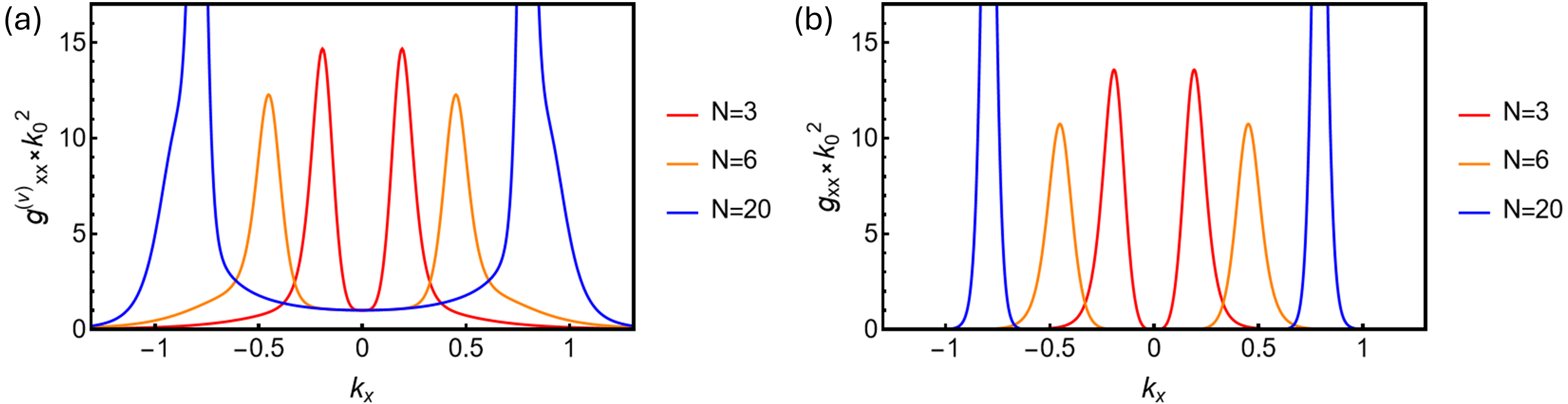
Figure S2: Contrasting the valence band QM of (a) the continuum model, $g^{(v)}_{xx}$ with (b) the two-band effective model, $\tilde{g}^{(v)}_{xx}$ along $k_{y}=0$, for $N=3,6,20$ at $m=0.01\gamma_{1}$.

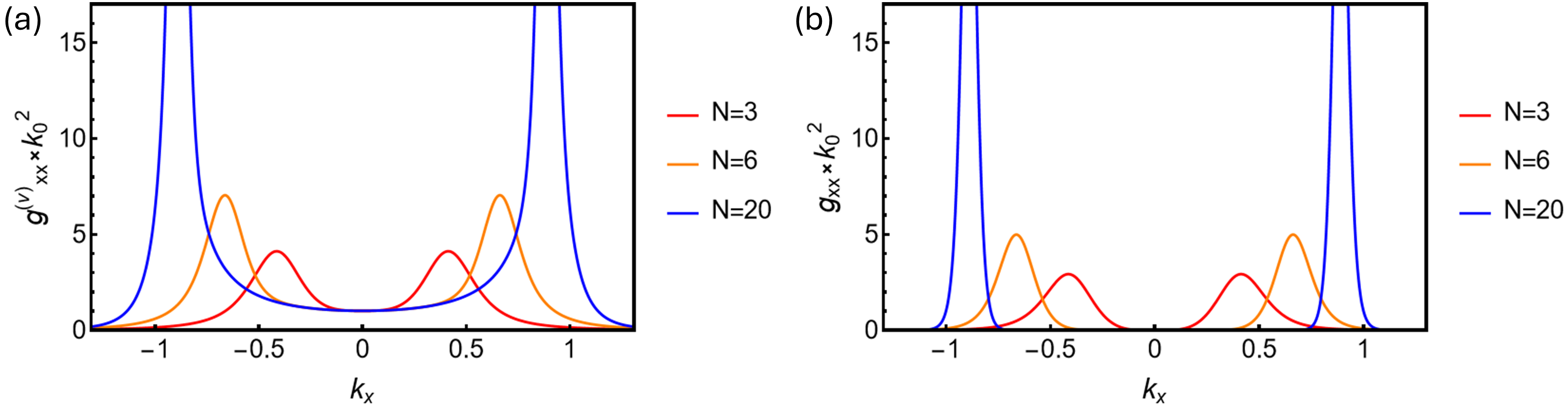
Figure S3: Same as Fig. S2, but with a larger surface potential $m=0.1\gamma_{1}$.

To study the dependence of $g_{\mu\nu}^{(v)}$ and $\tilde{g}_{\mu\nu}^{(v)}$ on $m$, in Fig. S3 we plot these QMs for a larger surface potential $m=0.1\gamma_{1}$. Firstly, we notice that the QM at the center does not depend on $m$. Secondly, a larger $m$ leads to a larger bandgap between the two surface bands, making the QM peaks at $k_{h}$ less singular [110]. This is because these peaks are mainly contributed by the interband (band-resolved) quantum metric, which can be written as

$$g^{(vc)}_{\mu\nu}(\textbf{k})=-\text{Re}\langle\partial_{\mu}\psi^{(v)}_{\textbf{k}}|\psi^{(c)}_{\textbf{k}}\rangle\langle\psi^{(c)}_{\textbf{k}}|\partial_{\nu}\psi^{(v)}_{\textbf{k}}\rangle=-\text{Re}\frac{\langle\psi^{(v)}_{\textbf{k}}|\partial_{\mu}H(\textbf{k})|\psi^{(c)}_{\textbf{k}}\rangle\langle\psi^{(c)}_{\textbf{k}}|\partial_{\nu}H(\textbf{k})|\psi^{(v)}_{\textbf{k}}\rangle}{(\varepsilon_{c,\textbf{k}}-\varepsilon_{v,\textbf{k}})^{2}}\propto\frac{1}{(\varepsilon_{c,\textbf{k}}-\varepsilon_{v,\textbf{k}})^{2}}.$$ (S18)

This inversely proportional relation determines how these peaks vary with the bandgap. Note that the bandgap $|\varepsilon_{c,\textbf{k}}-\varepsilon_{v,\textbf{k}}|$ is k-dependent, with a maximum $2m$ at the center and decreases as it goes to the rim (this is similar to the k-dependence of the superconducting order parameter in the band basis, $\Delta_{v,\textbf{k}}$). This explains why the variation of the QM peak with $m$ for smaller $N$ is stronger than for larger $N$-layer RG, e.g., the $N=20$ peaks does not change much but $N=3$ peaks change a lot.

Lastly, another important feature is that the hybridization momentum $k_{h}$ slightly increases with increasing $m$. This means that when the displacement field is applied, the central region where the QGT is uniform and the local inequality between QM and Berry curvature is saturated expands, as can be seen from Figs. S2(a) and S3(a). For large $m$, we compute $k_{h}$ by finding the maxima of Eq. (S17), giving

$$k_{h}=\bigg{(}\frac{N-1}{N+1}\bigg{)}^{1/N}m^{1/N}\approx m^{1/N}.$$ (S19)

Since the two-band model does not work near $k=0$, Eq. (S19) is only valid for large $m$.

II.3 S2.3 Continuum model with long-range couplings

When long-range couplings $\gamma_{2}-\gamma_{4}$ are present, the quantum geometry is only changed quantitatively, especially when a surface potential $m$ is applied (as discussed in the main text). In Fig. S4(a), we plot the QM of the valence band for the continuum model with $\gamma_{2}-\gamma_{4}$ couplings and surface potential $m=0.01\gamma_{1}$. We also examine the saturation criteria $|B^{(v)}|/\text{Tr}g^{(v)}$ in Fig. S4(b) and find it is close to 1 in most of the region confined by $k<k_{h}$ for large $N$. In Fig. S5 we show the same plots for a larger $m=0.1\gamma_{1}$. As $m$ increases, the inequality is better saturated in a wider region.

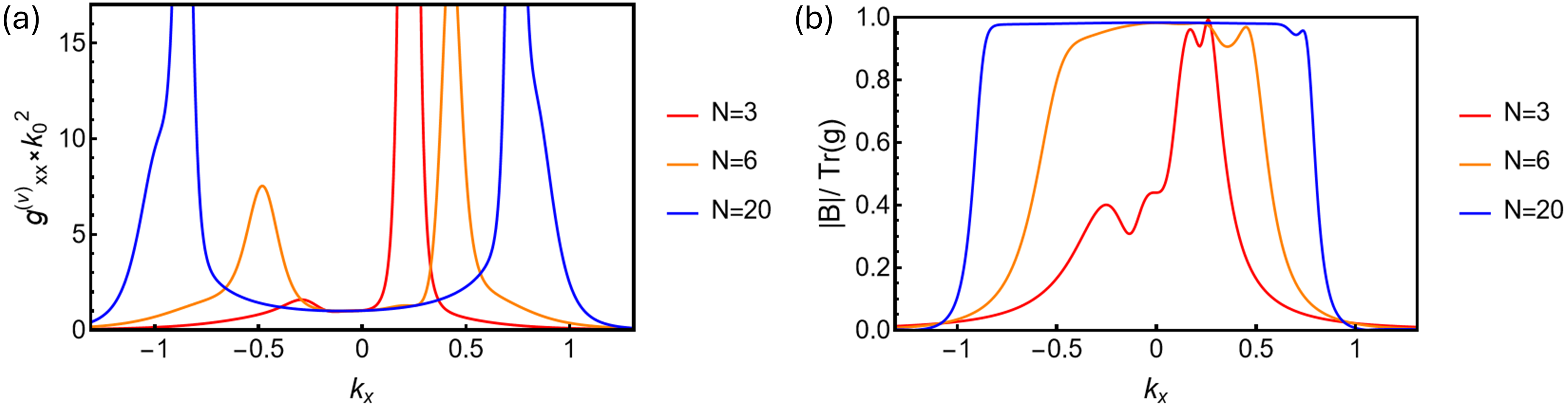
Figure S4: (a) Valence band quantum metric of the continuum model with $\gamma_{2}-\gamma_{4}$ couplings and surface potential $m=0.01\gamma_{1}$ (parameters explained in Sec. S1). (b) The ratio of saturation $|B^{(v)}|/\text{Tr}g^{(v)}$ for the valence surface band at $m=0.01\gamma_{1}$.

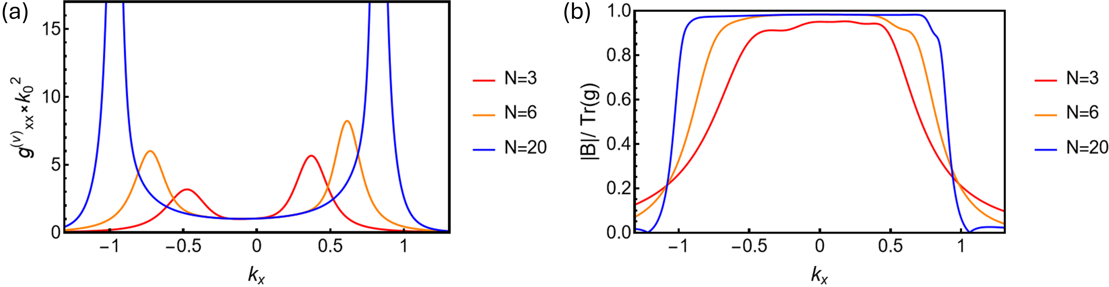
Figure S5: Same as Fig. S4 but with a larger surface potential $m=0.1\gamma_{1}$.

III S3: Self-consistency equations and superfluid weight calculation

In this section we present some details for calculating the superconducting gap and superfluid weight.

III.1 S3.1: Self-consistent gap equation and electron number equation

The onsite attractive density-density interaction for the RG is

$$\hat{H}_{I}=-U\sum_{\textbf{R},\alpha}\hat{n}_{\textbf{R}\alpha\uparrow}\hat{n}_{\textbf{R}\alpha\downarrow}=-\frac{U}{N_{c}}\sum_{\textbf{k}\textbf{k}^{\prime}\textbf{q},\alpha}c_{\textbf{k}+\textbf{q},\alpha\uparrow}^{\dagger}c_{-\textbf{k}+\textbf{q},\alpha\downarrow}^{\dagger}c_{-\textbf{k}^{\prime}+\textbf{q},\alpha\downarrow}c_{\textbf{k}^{\prime}+\textbf{q},\alpha\uparrow}$$ (S20)

with $U>0$. After mean-field decoupling, it leads to an intra-orbital pairing matrix which is diagonal in the orbital basis $\hat{\Delta}=\text{diag}(\Delta_{\alpha})$ ($\alpha$ running over the $2N$ orbitals) and

$$\Delta_{\alpha}\equiv-U\langle c_{\textbf{R}\alpha\downarrow}c_{\textbf{R}\alpha\uparrow}\rangle=-\frac{2U}{N_{c}}\sum_{\textbf{k}\in\Lambda_{K}}\langle c_{-\textbf{k}\alpha\downarrow}c_{\textbf{k}\alpha\uparrow}\rangle,$$ (S21)

where the sum over k is over a cutoff region $\Lambda_{K}$ near $K$ and the factor 2 counts the valley degeneracy. For a weak interaction $U\ll\gamma_{1}$, it is a valid approximation that the only nonzero order parameters are $\Delta_{1\text{A}}$ and $\Delta_{N\text{B}}$. Therefore, $\hat{\Delta}=\text{diag}(\Delta_{1\text{A}},0,0,..,0,\Delta_{N\text{B}})$.

The Bogoliubov-de-Gennes (BdG) equation

$$H_{\text{BdG}}(\textbf{k})\phi_{i}(\textbf{k})=E_{i,\textbf{k}}\phi_{i}(\textbf{k})$$ (S22)

can be diagonalized numerically. Here $i$ labels the $4N$ Bogoliubov bands and

$$H_{\text{BdG}}(\textbf{k})=\begin{pmatrix}H^{\uparrow}(\textbf{k})-\mu&\hat{\Delta}\\ \hat{\Delta}&-[H^{\downarrow T}(-\textbf{k})-\mu]\end{pmatrix}.$$ (S23)

By time-reversal symmetry, $H^{\uparrow}(\textbf{k})=H^{\downarrow T}(-\textbf{k})\equiv H(\textbf{k})$ with $H(\textbf{k})$ the $2N$ by $2N$ continuum model Hamiltonian of $N$-layer RG. For the spinor components of eigenstate $\phi_{i}$, we label the spin-$\uparrow$ and $\downarrow$ component of orbital $\alpha$ by $\alpha$ and $\bar{\alpha}$, respectively. Then Eq. (S21) becomes

$$\Delta_{\alpha}=-\frac{2U}{N_{c}}\sum_{\textbf{k}\in\Lambda_{K}}\sum_{i=1}^{4N}\phi_{i\bar{\alpha}}(\textbf{k})^{*}\phi_{i\alpha}(\textbf{k})n_{i}(\textbf{k}),$$ (S24)

where $n_{i}(\textbf{k})=\frac{1}{1+\text{exp}(\beta E_{i,\textbf{k}})}$ is the Fermi-Dirac function.

Similarly, the electron number equation in terms of eigenstates $\phi_{i}$ is

$$\begin{split}N_{e}=&2\sum_{\textbf{k}\in\Lambda_{K}}\sum_{\alpha}(\langle c_{\textbf{k}\alpha\uparrow}^{\dagger}c_{\textbf{k}\alpha\uparrow}\rangle+\langle c_{-\textbf{k}\alpha\downarrow}^{\dagger}c_{-\textbf{k}\alpha\downarrow}\rangle)\\ =&2\sum_{\textbf{k}\in\Lambda_{K}}\sum_{\alpha}\sum_{i=1}^{4N}\big{\{}n_{i}(\textbf{k})|\phi_{i\alpha}(\textbf{k})|^{2}+[1-n_{i}(\textbf{k})]|\phi_{i\bar{\alpha}}(\textbf{k})|^{2}\big{\}}.\end{split}$$ (S25)

It is convenient to measure the electron density from half-filling, where the total number of electrons is

$$N_{e,0}=2\sum_{\textbf{k}\in\Lambda_{K}}\sum_{\alpha}(\frac{1}{2}+\frac{1}{2})=2\sum_{\textbf{k}\in\Lambda_{K}}\sum_{\alpha}\sum_{i=1}^{4N}|\phi_{i\bar{\alpha}}(\textbf{k})|^{2}.$$ (S26)

Then, the measured electron number is

$$\delta N_{e}\equiv N_{e}-N_{e,0}=2\sum_{\textbf{k}\in\Lambda_{K}}\sum_{\alpha}\sum_{i=1}^{4N}n_{i}(\textbf{k})\big{[}|\phi_{i\alpha}(\textbf{k})|^{2}-|\phi_{i\bar{\alpha}}(\textbf{k})|^{2}\big{]}.$$ (S27)

The electron density $n_{e}\equiv\delta N_{e}/S$ ($S$ is the sample area) is in the units of $\text{cm}^{-2}$ [note that the momentum is in the units of $k_{0}=\gamma_{1}/(\hbar v_{f})=0.39\text{ eV}/(6.58\times 10^{-16}\text{ eV}\cdot\text{s}\times 10^{6}\text{ m/s})=5.9\times 10^{6}\text{ cm}^{-1}$].

When the two surface bands of the RG are gapped (by surface potential $m$) with a gap larger than $\Delta_{\alpha}$, and the superconducting state is doped to only one band (e.g., the valence surface band $v$), the single-band projection becomes valid. Therefore, the summation over the $4N$ Bogoliubov bands in Eq. (S24) and S27 can be replaced with summation over only the quasiparticle and quasihole bands associated with the valence band, $v+$ and $v-$, i.e. $\sum_{i=1}^{4N}\rightarrow\sum_{i=v+,v-}$.

III.2 S3.2: General superfluid weight formula

We use the grand potential formalism [75] to compute the superfluid weight for multilayer RG numerically. The superfluid weight tensor is the second total derivative of the free energy density with half of the Cooper pair center of mass momentum q, $D_{s,\mu\nu}=\frac{1}{S}\frac{\,\mathrm{d}^{2}F(\textbf{q})}{\,\mathrm{d}q_{\mu}\,\mathrm{d}q_{\nu}}\big{|}_{\textbf{q}=0}$ (we set $e=\hbar=1$; for convenience we set the sample area $S=1$ hereafter). Under TRS, using the relation between free energy and grand potential, $F(\textbf{q})=\Omega(\textbf{q},\hat{\Delta}_{\textbf{q}},\hat{\Delta}_{\textbf{q}}^{*},\mu_{\textbf{q}})+\mu_{\textbf{q}}N_{e}$ where the q-dependence of $\hat{\Delta}_{\textbf{q}},\mu_{\textbf{q}}$ arise from self-consistency equations (the electron number $N_{e}$ is fixed for different q), the superfluid weight can be expressed as [75, 92]:

$$D_{s,\mu\nu}=\bigg{[}\frac{\partial^{2}\Omega}{\partial q_{\mu}\partial q_{\nu}}-\sum_{\alpha,\beta}\frac{\,\mathrm{d}\Delta^{I}_{\textbf{q},\alpha}}{\,\mathrm{d}q_{\mu}}\frac{\partial^{2}\Omega}{\partial\Delta^{I}_{\textbf{q},\alpha}\partial\Delta^{I}_{\textbf{q},\beta}}\frac{\,\mathrm{d}\Delta^{I}_{\textbf{q},\beta}}{\,\mathrm{d}q_{\nu}}\bigg{]}\bigg{|}_{\textbf{q}=0}.$$ (S28)

Here, the second term of Eq. (S28) makes $D_{s,\mu\nu}$ gauge-invariant with respect to the position choices $\textbf{x}_{\alpha}$ of different orbitals $\alpha$ ($\hat{\Delta}_{\textbf{q}}=\text{diag}(\Delta_{\textbf{q},\alpha})$ denotes the pairing matrix of the finite-q supercurrent state). Here $\Delta^{I}_{\textbf{q},\alpha}$ is the imaginary part of $\Delta_{\textbf{q},\alpha}$, which is 0 at $\textbf{q}=0$ since all $\Delta_{\alpha}$ are real by virtue of TRS. TRS also implies that $\frac{\,\mathrm{d}\Delta_{\textbf{q},\alpha}}{\,\mathrm{d}q_{\mu}}|_{\textbf{q}=0}=i\frac{\,\mathrm{d}\Delta^{I}_{\textbf{q},\alpha}}{\,\mathrm{d}q_{\mu}}|_{\textbf{q}=0}=-\frac{\,\mathrm{d}\Delta_{\textbf{q},\alpha}^{*}}{\,\mathrm{d}q_{\mu}}|_{\textbf{q}=0}$. Taking into account a prefactor $1/(\mathcal{A}k_{0}^{2})=54.9$, where $\mathcal{A}=5.24\times 10^{-16}$cm² is the unit cell area coming from $1/S=1/(N_{c}\mathcal{A})$, the calculated $D_{s}$ has the dimension of energy. In other words, the final superfluid weight is the calculated value multiplied by a factor of $54.9\frac{e^{2}}{\hbar^{2}}$. Here, we compute the first term of Eq. (S28); the second term is calculated in Sec. S3.4.

The BdG Hamiltonian for the supercurrent state is

$$H_{\text{BdG}}(\textbf{k},\textbf{q})=\begin{pmatrix}H^{\uparrow}(\textbf{k}+\textbf{q})-\mu_{\textbf{q}}I_{2N}&\hat{\Delta}_{\textbf{q}}\\ \hat{\Delta}_{\textbf{q}}&-[H^{\downarrow\,T}(-\textbf{k}+\textbf{q})-\mu_{\textbf{q}}I_{2N}]\end{pmatrix},$$ (S29)

and the second-quantized total mean-field Hamiltonian is

$$\hat{H}_{\text{MF}}(\textbf{q})=\sum_{\textbf{k}\in\text{BZ}}\big{\{}\textbf{C}_{\textbf{k},\textbf{q}}^{\dagger}H_{\text{BdG}}(\textbf{k},\textbf{q})\textbf{C}_{\textbf{k},\textbf{q}}+\text{Tr}[H^{\downarrow}(-\textbf{k}+\textbf{q})-\mu_{\textbf{q}}I_{2N}]\big{\}}+\frac{N_{c}}{U}\sum_{\alpha}|\Delta_{\textbf{q},\alpha}|^{2},$$ (S30)

where $\textbf{C}_{\textbf{k},\textbf{q}}=(c_{\textbf{k}+\textbf{q},1\text{A},\uparrow},..,c_{-\textbf{k}+\textbf{q},1\text{A},\downarrow}^{\dagger},..)^{T}$, $I_{2N}$ is the $2N$-dimensional identity matrix and k runs over the entire Brillouin zone (BZ). Let $\hat{E}_{\textbf{k}}(\textbf{q})$ denote the diagonal matrix of the spectrum of $H_{\text{BdG}}(\textbf{k},\textbf{q})$ by diagonalization, then at temperature $T=1/\beta$ [75],

$$\Omega(\textbf{q},\hat{\Delta}_{\textbf{q}},\hat{\Delta}_{\textbf{q}}^{*},\mu_{\textbf{q}})=-\frac{1}{\beta}\ln\text{Tr}\{e^{-\beta\hat{H}_{\text{MF}}(\textbf{q})}\}=-\frac{1}{2\beta}\sum_{\textbf{k}\in\text{BZ}}\text{Tr}\ln[2+2\cosh\beta\hat{E}_{\textbf{k}}(\textbf{q})]+\frac{N_{c}}{U}\sum_{\alpha}|\Delta_{\textbf{q},\alpha}|^{2}+\text{const.}$$ (S31)

When computing the first term of Eq. (S28), we treat $\hat{\Delta}_{\textbf{q}}$ and $\mu_{\textbf{q}}$ as q-independent in Eq. (S31).

The Fermi surfaces of RG at valleys $K$ and $K^{\prime}$ are small compared to the entire Brillouin zone. Therefore, it is necessary to convert Eq. (S31) into a summation that converges in a finite cutoff regions at the two valleys. Note that the conduction (valence) surface band has a particle (hole)-like Fermi surface, i.e., as k is far from the cutoff regions, asymptotically

$$E_{c\pm,\textbf{k}}(\textbf{q})\rightarrow\pm\xi_{c,\textbf{k}\pm\textbf{q}},\,\,\,E_{v\pm,\textbf{k}}(\textbf{q})\rightarrow\mp\xi_{v,\textbf{k}\mp\textbf{q}},$$ (S32)

where $\xi_{c(v),\textbf{k}}=\varepsilon_{c(v),\textbf{k}}-\mu$, with $\varepsilon_{c(v),\textbf{k}}$ the electronic band dispersion of the conduction (valence) band. Here $E_{c(v)\pm,\textbf{k}}$ are the quasiparticle (+) and quasihole (-) band spectra associated with $c$ and $v$ bands in the diagonal entries of $\hat{E}_{\textbf{k}}(\textbf{q})$. We then transform the grand potential $\Omega$ by adding a q-independent boundary term: $\Omega(\textbf{q},\hat{\Delta}_{\textbf{q}},\hat{\Delta}_{\textbf{q}}^{*},\mu_{\textbf{q}})+\Omega_{0}\rightarrow\Omega(\textbf{q},\hat{\Delta}_{\textbf{q}},\hat{\Delta}_{\textbf{q}}^{*},\mu_{\textbf{q}})$ (this process corresponds to “subtracting the supercurrent in the normal state” in literature [111, 27]). Specifically, we break each integral term (due to the trace of the diagonal matrix $\hat{E}_{\textbf{k}}(\textbf{q})$) of Eq. (S31), which integrates k over the entire BZ, into a sum of integrals inside and outside $\Lambda_{K}$. e.g., for the $E_{c+,\textbf{k}}(\textbf{q})$ term:

$$\begin{split}\sum_{\textbf{k}\in\text{BZ}}\ln[2+2\cosh\beta E_{c+,\textbf{k}}(\textbf{q})]=&\sum_{\textbf{k}\in\Lambda_{K}}\ln[2+2\cosh\beta E_{c+,\textbf{k}}(\textbf{q})]+\sum_{\textbf{k}\in\Lambda_{K^{\prime}}}\ln[2+2\cosh\beta E_{c+,\textbf{k}}(\textbf{q})]+\sum_{\textbf{k}\notin\Lambda_{K}\text{ or }\Lambda_{K^{\prime}}}\ln[2+2\cosh\beta E_{c+,\textbf{k}}(\textbf{q})]\\ =&2\sum_{\textbf{k}\in\Lambda_{K}}\ln[2+2\cosh\beta E_{c+,\textbf{k}}(\textbf{q})]+\sum_{\textbf{k}\notin\Lambda_{K}\text{ or }\Lambda_{K^{\prime}}}\ln[2+2\cosh\beta E_{c+,\textbf{k}}(\textbf{q})]\\ =&2\sum_{\textbf{k}\in\Lambda_{K}}\ln[2+2\cosh\beta E_{c+,\textbf{k}}(\textbf{q})]+\sum_{\textbf{k}\notin\Lambda_{K}\text{ or }\Lambda_{K^{\prime}}}\ln[2+2\cosh\beta\xi_{c,\textbf{k}+\textbf{q}}]\\ =&2\sum_{\textbf{k}\in\Lambda_{K}}\ln\frac{2+2\cosh\beta E_{c+,\textbf{k}}(\textbf{q})}{2+2\cosh\beta\xi_{c,\textbf{k}+\textbf{q}}}+\sum_{\textbf{k}\in\text{BZ}}\ln[2+2\cosh\beta\xi_{c,\textbf{k}+\textbf{q}}].\end{split}$$ (S33)

Here $\Lambda_{K^{\prime}}$ refers to the cutoff region at valley $K^{\prime}$ which is of the same size as $\Lambda_{K}$; to get the second line, we used valley degeneracy; to get the third line, we used the asymptotic relation Eq. (S32); to get the last line, we used partial integral. The last term in the last line above is q-independent as it integrates over the entire BZ, so it contributes to the boundary term $\Omega_{0}$. We then obtain the following transformed grand potential which integrates over the region $\Lambda_{K}$ only:

$$\Omega(\textbf{q},\hat{\Delta}_{\textbf{q}},\hat{\Delta}_{\textbf{q}}^{*},\mu_{\textbf{q}})=-\frac{1}{\beta}\sum_{\textbf{k}\in\Lambda_{K}}\bigg{[}\ln\frac{1+\cosh\beta E_{c+,\textbf{k}}(\textbf{q})}{1+\cosh\beta\xi_{c,\textbf{k}+\textbf{q}}}+\ln\frac{1+\cosh\beta E_{c-,\textbf{k}}(\textbf{q})}{1+\cosh\beta\xi_{c,\textbf{k}-\textbf{q}}}+\ln\frac{1+\cosh\beta E_{v+,\textbf{k}}(\textbf{q})}{1+\cosh\beta\xi_{v,\textbf{k}-\textbf{q}}}+\ln\frac{1+\cosh\beta E_{v-,\textbf{k}}(\textbf{q})}{1+\cosh\beta\xi_{v,\textbf{k}+\textbf{q}}}\bigg{]}.$$ (S34)

At $T=0$ it can be replaced with a simple integral

$$\Omega(\textbf{q},\hat{\Delta}_{\textbf{q}},\hat{\Delta}_{\textbf{q}}^{*},\mu_{\textbf{q}})=2\sum_{\textbf{k}\in\Lambda_{K}}\big{\{}\big{[}E_{c-,\textbf{k}}(\textbf{q})+\xi_{c,\textbf{k}-\textbf{q}}\big{]}+\big{[}E_{v-,\textbf{k}}(\textbf{q})-\xi_{v,\textbf{k}+\textbf{q}}\big{]}\big{\}}.$$ (S35)

If in the superconducting state, e.g., only the valence band is doped, i.e., the chemical potential is at the valence band and the superconducting gap is smaller than the bandgaps between the valence band and all other bands, then only the last two terms in Eq. (S34) and (S35) are nonzero.

III.3 S3.3: Separation into the conventional and geometric contributions

We separate the first term of Eq. (S28) into the conventional and geometric contributions, $\frac{\partial^{2}\Omega}{\partial q_{\mu}\partial q_{\nu}}\big{|}_{\textbf{q}=0}=D_{s,\mu\nu}^{\text{conv}}+D_{s,\mu\nu}^{\text{geo}}$. When the valence surface band is doped, single-band projection leads to the BdG Hamiltonian in the band basis

$$H_{\text{BdG}}(\textbf{k},\textbf{q})=\begin{pmatrix}\xi_{v,\textbf{k}+\textbf{q}}&\Delta_{v,\textbf{k}}(\textbf{q})\\ \Delta_{v,\textbf{k}}(\textbf{q})^{*}&-\xi_{v,\textbf{k}-\textbf{q}}\end{pmatrix},$$ (S36)

where $\Delta_{v,\textbf{k}}(\textbf{q})=\langle\psi^{(v)}_{\textbf{k}+\textbf{q}}|\hat{\Delta}|\psi^{(v)}_{\textbf{k}-\textbf{q}}\rangle$ (here $\hat{\Delta}$ and $\mu$ are taken as q-independent). The Bogoliubov spectra of Eq. (S36) are

$$E_{v\pm,\textbf{k}}(\textbf{q})=\frac{1}{2}\big{[}(\xi_{v,\textbf{k}+\textbf{q}}-\xi_{v,\textbf{k}-\textbf{q}})\pm\sqrt{(\xi_{v,\textbf{k}+\textbf{q}}+\xi_{v,\textbf{k}-\textbf{q}})^{2}+4|\Delta_{v,\textbf{k}}(\textbf{q})|^{2}}\big{]},$$ (S37)

which have the following derivatives

$$\partial_{q_{\mu}}E_{v\pm,\textbf{k}}(\textbf{q})|_{\textbf{q}=0}=\partial_{\mu}\xi_{v,\textbf{k}}\pm\frac{1}{E_{v,\textbf{k}}}\partial_{q_{\mu}}|\Delta_{v,\textbf{k}}(\textbf{q})|^{2}\big{|}_{\textbf{q}=0}=\partial_{\mu}\xi_{v,\textbf{k}},$$ (S38)

$$\partial_{q_{\mu}}\partial_{q_{\nu}}E_{v\pm,\textbf{k}}(\textbf{q})|_{\textbf{q}=0}=\pm\bigg{[}\frac{\xi_{v,\textbf{k}}}{E_{v,\textbf{k}}}\partial_{\mu}\partial_{\nu}\xi_{v,\textbf{k}}+\frac{1}{2E_{v,\textbf{k}}}\partial_{q_{\mu}}\partial_{q_{\nu}}|\Delta_{v,\textbf{k}}(\textbf{q})|^{2}\big{|}_{\textbf{q}=0}\bigg{]},$$ (S39)

and where $E_{v,\textbf{k}}\equiv\sqrt{\xi_{v,\textbf{k}}^{2}+\Delta_{v,\textbf{k}}(0)^{2}}$ is the quasiparticle energy at $\textbf{q}=0$. In Eq. (S38), the second term vanishes because the pairing matrix $\hat{\Delta}$ is Hermitian as a result of TRS. Using these when taking the derivative of Eq. (S34), we can isolate the two contributions

$$\begin{split}&D_{s,\mu\nu}^{\text{conv}}=-2\sum_{\textbf{k}\in\Lambda_{K}}\bigg{[}\bigg{(}\frac{\xi_{v,\textbf{k}}}{E_{v,\textbf{k}}}\tanh\frac{\beta E_{v,\textbf{k}}}{2}-\tanh\frac{\beta\xi_{v,\textbf{k}}}{2}\bigg{)}\partial_{\mu}\partial_{\nu}\xi_{v,\textbf{k}}+\frac{\beta}{2}\bigg{(}\text{sech}^{2}\frac{\beta E_{v,\textbf{k}}}{2}-\text{sech}^{2}\frac{\beta\xi_{v,\textbf{k}}}{2}\bigg{)}\partial_{\mu}\xi_{v,\textbf{k}}\partial_{\nu}\xi_{v,\textbf{k}}\bigg{]},\\ &D_{s,\mu\nu}^{\text{geo}}=-2\sum_{\textbf{k}\in\Lambda_{K}}\frac{1}{2E_{v,\textbf{k}}}\tanh\frac{\beta E_{v,\textbf{k}}}{2}\partial_{q_{\mu}}\partial_{q_{\nu}}|\Delta_{v,\textbf{k}}(\textbf{q})|^{2}\big{|}_{\textbf{q}=0},\end{split}$$ (S40)

At $T=0$, using $\lim_{\beta\rightarrow+\infty}\text{sech}^{2}\frac{\beta\xi_{v,\textbf{k}}}{2}=\frac{4}{\beta}\delta(\xi_{v,\textbf{k}})$, they reduce to

$$\begin{split}&D_{s,\mu\nu}^{\text{conv}}(T=0)=-2\sum_{\textbf{k}\in\Lambda_{K}}\bigg{\{}\bigg{[}\frac{\xi_{v,\textbf{k}}}{E_{v,\textbf{k}}}-\text{sgn}(\xi_{v,\textbf{k}})\bigg{]}\partial_{\mu}\partial_{\nu}\xi_{v,\textbf{k}}-2\delta(\xi_{v,\textbf{k}})\partial_{\mu}\xi_{v,\textbf{k}}\partial_{\nu}\xi_{v,\textbf{k}}\bigg{\}}\equiv 2\sum_{\textbf{k}\in\Lambda_{K}}f_{\mu\nu}^{\text{conv}},\\ &D_{s,\mu\nu}^{\text{geo}}(T=0)=-2\sum_{\textbf{k}\in\Lambda_{K}}\frac{1}{2E_{v,\textbf{k}}}\partial_{q_{\mu}}\partial_{q_{\nu}}|\Delta_{v,\textbf{k}}(\textbf{q})|^{2}\big{|}_{\textbf{q}=0}\equiv 2\sum_{\textbf{k}\in\Lambda_{K}}f_{\mu\nu}^{\text{geo}}.\end{split}$$ (S41)

Here the $\text{sgn}(\xi_{v,\textbf{k}})$ and $\delta(\xi_{v,\textbf{k}})$ terms combine to give a boundary term, making $D_{s,\mu\nu}^{\text{conv}}(T=0)$ consistent with the usual integral formula over the entire Brillouin zone with the integrand $-\frac{\xi_{v,\textbf{k}}}{E_{v,\textbf{k}}}\partial_{\mu}\partial_{\nu}\xi_{v,\textbf{k}}$. An equivalent and more convenient form is

$$D_{s,\mu\nu}^{\text{conv}}(T=0)=-2\sum_{\textbf{k}\in\Lambda_{K}}\bigg{(}\frac{\xi_{v,\textbf{k}}}{E_{v,\textbf{k}}}+1\bigg{)}\partial_{\mu}\partial_{\nu}\xi_{v,\textbf{k}}.$$ (S42)

Here attention is needed as the integrand $f_{\mu\nu}^{\text{conv}}$ depends on the choice of the boundary term $\Omega_{0}$. A physically meaningful integrand satisfies $f_{\mu\nu}^{\text{conv}}(\textbf{k})\propto\partial_{\mu}\xi_{v,\textbf{k}}$ and vanishes outside the cutoff region, as we are working with a continuum model. The term $f_{\mu\nu}^{\text{geo}}$ has the following expression [93]:

$$\begin{split}-\frac{1}{2E_{v,\textbf{k}}}\partial_{q_{\mu}}\partial_{q_{\nu}}|\Delta_{c,\textbf{k}}(\textbf{q})|^{2}\big{|}_{\textbf{q}=0}=&-\frac{1}{2E_{v,\textbf{k}}}\text{Tr}\big{\{}\partial_{\mu}\partial_{\nu}P^{(v)}_{\textbf{k}}\hat{\Delta}P^{(v)}_{\textbf{k}}\hat{\Delta}^{\dagger}+P^{(v)}_{\textbf{k}}\hat{\Delta}\partial_{\mu}\partial_{\nu}P^{(v)}_{\textbf{k}}\hat{\Delta}^{\dagger}-\partial_{\mu}P^{(v)}_{\textbf{k}}\hat{\Delta}\partial_{\nu}P^{(v)}_{\textbf{k}}\hat{\Delta}^{\dagger}-\partial_{\nu}P^{(v)}_{\textbf{k}}\hat{\Delta}\partial_{\mu}P^{(v)}_{\textbf{k}}\hat{\Delta}^{\dagger}\big{\}}\\ =&-\frac{1}{E_{v,\textbf{k}}}\text{Tr}\big{\{}\partial_{\mu}\partial_{\nu}P^{(v)}_{\textbf{k}}\hat{\Delta}P^{(v)}_{\textbf{k}}\hat{\Delta}-\partial_{\mu}P^{(v)}_{\textbf{k}}\hat{\Delta}\partial_{\nu}P^{(v)}_{\textbf{k}}\hat{\Delta}\big{\}}.\end{split}$$ (S43)

One can show that $f_{\mu\nu}^{\text{geo}}$ of RG surface bands has similar features in k space as the QM $g^{(v)}_{\mu\nu}$. Again, we consider the RG model with only $\gamma_{0},\gamma_{1}$ couplings and the $N\rightarrow\infty$ limit. Then $\hat{\Delta}=\text{diag}(0,...,0,\Delta_{N\text{B}})$ leads to

$$-\partial_{q_{\mu}}\partial_{q_{\nu}}|\Delta_{v,\textbf{k}}(\textbf{q})|^{2}\big{|}_{\textbf{q}=0}=-2\Delta_{N\text{B}}^{2}\big{[}\langle N\text{B}|\partial_{\mu}\partial_{\nu}P^{(v)}_{\textbf{k}}|N\text{B}\rangle\langle N\text{B}|P^{(v)}_{\textbf{k}}|N\text{B}\rangle-\langle N\text{B}|\partial_{\mu}P^{(v)}_{\textbf{k}}|N\text{B}\rangle\langle N\text{B}|\partial_{\nu}P^{(v)}_{\textbf{k}}|N\text{B}\rangle\big{]}.$$ (S44)

Using $\langle N\text{B}|P^{(v)}_{\textbf{k}}|N\text{B}\rangle=\frac{1-k^{2}}{k^{2}}e^{(\kappa+\kappa^{*})}$, we find

$$-\partial_{q_{\mu}}\partial_{q_{\nu}}|\Delta_{v,\textbf{k}}(\textbf{q})|^{2}\big{|}_{\textbf{q}=0}=4\Delta_{N\text{B}}^{2}[(1-k^{2})\delta_{\mu\nu}+2k_{\mu}k_{\nu}].$$ (S45)

When the chemical potential is aligned with the flat valence band, we have $E_{v,\textbf{k}}=\Delta_{v,\textbf{k}}=\Delta_{N\text{B}}(1-k^{2})$. Then

$$f_{\mu\nu}^{\text{geo}}(\textbf{k})=\frac{4\Delta_{N\text{B}}^{2}[(1-k^{2})\delta_{\mu\nu}+2k_{\mu}k_{\nu}]}{2\Delta_{N\text{B}}(1-k^{2})}=2\Delta_{N\text{B}}\bigg{(}\delta_{\mu\nu}+\frac{2}{1-k^{2}}k_{\mu}k_{\nu}\bigg{)}.$$ (S46)

At $k_{y}=0$ and $k_{x}\ll 1$,

$$f_{xx}^{\text{geo}}(k_{x},k_{y}=0)=2\Delta_{N\text{B}}\frac{1+k_{x}^{2}}{1-k_{x}^{2}}\simeq 2\Delta_{N\text{B}}\frac{1}{(1-k_{x}^{2})^{2}},$$ (S47)

which has a similar k-dependence as $g^{(v)}_{xx}$. Another way to analyze $f_{\mu\nu}^{\text{geo}}(\textbf{k})$ is to compute its eigenvalues and eigenvectors. The two eigenvalues are $d_{1}(\textbf{k})=2\Delta_{N\text{B}}$ and $d_{2}(\textbf{k})=2\Delta_{N\text{B}}\frac{1+k^{2}}{1-k^{2}}$, with eigenvectors $\textbf{v}_{1}=(-k_{y},k_{x})$ and $\textbf{v}_{2}=(k_{x},k_{y})$, respectively. At the center of the drumhead region, the supercurrent response is isotropic ($d_{1}=d_{2}$); as it moves away from the center, the local supercurrent response by a state with moentum k gets polarized to vector potential A that is parallel to k as $d_{2}>d_{1}$ (however, the total supercurrent after the k-space integral is not polarized to any particular direction), with the eigenvalue $d_{2}\propto\frac{1+k^{2}}{1-k^{2}}\simeq\frac{1}{(1-k^{2})^{2}}$.

III.4 S3.4: $U(1)\times...\times U(1)$ gauge-invariance and the term $D_{s}^{\Delta}$

After mean-field decoupling, the onsite interaction for the supercurrent state is

$$\hat{H}_{\text{MF}}^{(int)}(\textbf{q})=\sum_{\textbf{k},\alpha}(\Delta_{\textbf{q},\alpha}c_{\textbf{k}+\textbf{q},\alpha\uparrow}^{\dagger}c_{-\textbf{k}+\textbf{q},\alpha\downarrow}^{\dagger}+h.c.)+\frac{N_{c}}{U}\sum_{\alpha}|\Delta_{\textbf{q},\alpha}|^{2},$$ (S48)

where the order parameter is (using $c_{\textbf{k}\alpha\sigma}=\frac{1}{\sqrt{N_{c}}}\sum_{\textbf{k}}e^{-i\textbf{k}\cdot(\textbf{R}+\textbf{x}_{\alpha})}c_{\textbf{R}\alpha\sigma}$)

$$\Delta_{\textbf{q},\alpha}=-\frac{U}{N_{c}}\sum_{\textbf{k}}\langle c_{-\textbf{k}+\textbf{q},\alpha\downarrow}c_{\textbf{k}+\textbf{q},\alpha\uparrow}\rangle_{\textbf{q}}=-U\langle c_{\textbf{R}\alpha\downarrow}c_{\textbf{R}\alpha\uparrow}\rangle_{\textbf{q}}e^{-2i\textbf{q}\cdot(\textbf{R}+\textbf{x}_{\alpha})},$$ (S49)

with $\langle\rangle_{\textbf{q}}$ the average in the supercurrent state $\Psi_{\textbf{q}}$. Operator $c_{\textbf{k}\alpha\sigma}$ has a $U(1)$ gauge freedom, i.e., under the fictitious transformation $\textbf{x}_{\alpha}\rightarrow\textbf{x}_{\alpha}+\delta\textbf{x}_{\alpha}$, $c_{\textbf{k}\alpha\sigma}\rightarrow\widetilde{c}_{\textbf{k}\alpha\sigma}=c_{\textbf{k}\alpha\sigma}e^{-i\textbf{k}\cdot\delta\textbf{x}_{\alpha}}$. This is purely a gauge choice that does not affect the state $\Psi_{\textbf{q}}$, and therefore, $\langle c_{\textbf{R}\alpha\downarrow}c_{\textbf{R}\alpha\uparrow}\rangle_{\textbf{q}}$ is $\textbf{x}_{\alpha}$-independent. Then it is easy to check that Hamiltonian Eq. (S48) is invariant under this $U(1)\times...\times U(1)$ (the number of copies of $U(1)$ is equal to the number of nonzero order parameters in the orbital basis) gauge of the set of operators $\{c_{\textbf{k}\alpha\sigma}\}$; and the implication of the second term of Eq. (S28) (denoted as $D_{s}^{\Delta}$) is to make the total $D_{s}$ invariant with respect to this gauge (i.e., to the orbital-dependent local gauge transformations, or orbital embedding). Note that even without including $D_{s}^{\Delta}$, the result $D_{s}^{\text{conv}}+D_{s}^{\text{geo}}$ is gauge-invariant with respect to the orbital-independent $U(1)$ gauge transformation.

To compute $D_{s}^{\Delta}$, we write down the gap equation for the supercurrent state in the orbital basis:

$$\Delta_{\textbf{q},\alpha}=\frac{U}{N_{c}}\sum_{\textbf{k}\in\Lambda_{K}}\frac{\psi^{(v)*}_{\textbf{k}-\textbf{q},\alpha}\psi^{(v)}_{\textbf{k}+\textbf{q},\alpha}\Delta_{v,\textbf{k}}(\textbf{q})}{\sqrt{(\xi_{v,\textbf{k}+\textbf{q}}+\xi_{v,\textbf{k}-\textbf{q}})^{2}+4|\Delta_{v,\textbf{k}}(\textbf{q})|^{2}}}\bigg{(}\tanh\frac{\beta E_{v+,\textbf{k}}(\textbf{q})}{2}-\tanh\frac{\beta E_{v-,\textbf{k}}(\textbf{q})}{2}\bigg{)},$$ (S50)

where the Bogoliubov spectrum $E_{v\pm,\textbf{k}}(\textbf{q})$ are given by Eq. (S37). Computing the derivative of Eq. (S50) leads to an equation $\sum_{\beta}M_{\alpha\beta}\,\mathrm{d}_{\mu}\Delta_{\beta}=V_{\alpha,\mu}$ ($\,\mathrm{d}_{\mu}\Delta_{\beta}$ stands for $\frac{\,\mathrm{d}\Delta_{\textbf{q},\beta}}{\,\mathrm{d}q_{\mu}}\big{|}_{\textbf{q}=0}$), with [107]

$$M_{\alpha\beta}=\frac{\delta_{\alpha\beta}}{\Delta_{\alpha}}\sum_{\textbf{k}\in\Lambda_{K}}\frac{\Delta_{v,\textbf{k}}(0)}{E_{v\textbf{k}}}\tanh\frac{\beta E_{v\textbf{k}}}{2}|\psi^{(v)}_{\textbf{k},\beta}|^{2}-\sum_{\textbf{k}\in\Lambda_{K}}\frac{1}{E_{v\textbf{k}}}\tanh\frac{\beta E_{v\textbf{k}}}{2}|\psi^{(v)}_{\textbf{k},\alpha}|^{2}|\psi^{(v)}_{\textbf{k},\beta}|^{2},$$ (S51)

and

$$V_{\alpha,\mu}=\sum_{\textbf{k}\in\Lambda_{K}}\frac{1}{E_{v\textbf{k}}}\tanh\frac{\beta E_{v\textbf{k}}}{2}\big{[}(\psi^{(v)*}_{\textbf{k},\alpha}\partial_{\mu}\psi^{(v)}_{\textbf{k},\alpha}-\partial_{\mu}\psi^{(v)*}_{\textbf{k},\alpha}\psi^{(v)}_{\textbf{k},\alpha})\Delta_{v,\textbf{k}}(0)-|\psi^{(v)}_{\textbf{k},\alpha}|^{2}(\langle\psi^{(v)}_{\textbf{k}}|\hat{\Delta}|\partial_{\mu}\psi^{(v)}_{\textbf{k}}\rangle-\langle\partial_{\mu}\psi^{(v)}_{\textbf{k}}|\hat{\Delta}|\psi^{(v)}_{\textbf{k}}\rangle)\big{]}.$$ (S52)

Here $M_{\alpha\beta}=\frac{1}{2}\frac{\partial^{2}\Omega}{\partial\Delta_{\textbf{q},\alpha}^{I}\partial\Delta_{\textbf{q},\beta}^{I}}\big{|}_{\textbf{q}=0}$ and $V_{\alpha,\mu}=-\frac{\partial^{2}\Omega}{\partial\Delta_{\textbf{q},\alpha}^{*}\partial q_{\mu}}\big{|}_{\textbf{q}=0}$.

Using Eq. (S51), the diagonal entries of $M$ are

$$M_{\alpha\alpha}=\sum_{\textbf{k}\in\Lambda_{K}}\sum_{\beta\neq\alpha}|\psi^{(v)}_{\textbf{k},\alpha}|^{2}|\psi^{(v)}_{\textbf{k},\beta}|^{2}\frac{\Delta_{\beta}}{\Delta_{\alpha}}\frac{\tanh(\beta E_{v\textbf{k}}/2)}{E_{v\textbf{k}}}.$$ (S53)

Assuming that the only nonzero order parameters are $\Delta_{1\text{A}}$ and $\Delta_{N\text{B}}$, then $M_{\alpha\alpha}$ for these $\alpha\in\{1\text{B},...,N\text{A}\}$ diverge. However, $V_{\alpha,\mu}$ is finite [can be seen from Eq. (S52)], although $V_{\alpha,\mu}=\sum_{\beta}M_{\alpha\beta}\,\mathrm{d}_{\mu}\Delta_{\beta}$. The reason is that $\,\mathrm{d}_{\mu}\Delta_{\alpha}=0$ for these $(2N-2)$ orbitals. Expressing $D_{s,\mu\nu}^{\Delta}=2\sum_{\alpha}V_{\alpha,\mu}\,\mathrm{d}_{\nu}\Delta_{\alpha}$, we are convinced that $D_{s,\mu\nu}^{\Delta}$ is always finite.

This suggests that we can restrict the summation of orbitals in the second term of Eq. (S28) to summing over 1A and $N$B only:

$$D_{s,\mu\nu}^{\Delta}=-\sum_{\alpha,\beta=1\text{A},N\text{B}}\frac{\,\mathrm{d}\Delta^{I}_{\textbf{q},\alpha}}{\,\mathrm{d}q_{\mu}}\frac{\partial^{2}\Omega}{\partial\Delta^{I}_{\textbf{q},\alpha}\partial\Delta^{I}_{\textbf{q},\beta}}\frac{\,\mathrm{d}\Delta^{I}_{\textbf{q},\beta}}{\,\mathrm{d}q_{\nu}}\bigg{|}_{\textbf{q}=0}=2\sum_{\alpha,\beta=1\text{A},N\text{B}}\,\mathrm{d}_{\mu}\Delta_{\alpha}M_{\alpha\beta}\,\mathrm{d}_{\nu}\Delta_{\beta}.$$ (S54)

Let us denote the restriction of the matrix $M$ to these two orbitals as $M_{R}$ (a 2 by 2 matrix), and similarly, the vector $V$ to these two orbitals as $V_{R}$ (a 2-dimensional vector). The matrix $M_{R}$ has a kernel eigenvector $\textbf{v}_{0}=(\Delta_{1\text{A}},\Delta_{N\text{B}})$, which enables us to eliminate, e.g., the second row and column of $M_{R}$ and the second component of $V_{R}$. Finally, this gives the simple expression

$$D_{s,\mu\nu}^{\Delta}=2\frac{V_{1\text{A},\mu}V_{1\text{A},\nu}}{M_{1\text{A},1\text{A}}}.$$ (S55)

where

$$M_{1\text{A},1\text{A}}=\sum_{\textbf{k}\in\Lambda_{K}}|\psi^{(v)}_{\textbf{k},1\text{A}}|^{2}|\psi^{(v)}_{\textbf{k},N\text{B}}|^{2}\frac{\Delta_{N\text{B}}}{\Delta_{1\text{A}}}\frac{\tanh(\beta E_{v\textbf{k}}/2)}{E_{v\textbf{k}}}$$ (S56)

and

$$V_{1\text{A},\mu}=\sum_{\textbf{k}\in\Lambda_{K}}\frac{\Delta_{N\text{B}}}{E_{v\textbf{k}}}\tanh\frac{\beta E_{v\textbf{k}}}{2}\big{[}|\psi^{(v)}_{\textbf{k},N\text{B}}|^{2}(\psi^{(v)*}_{\textbf{k},1\text{A}}\partial_{\mu}\psi^{(v)}_{\textbf{k},1\text{A}}-\partial_{\mu}\psi^{(v)*}_{\textbf{k},1\text{A}}\psi^{(v)}_{\textbf{k},1\text{A}})-|\psi^{(v)}_{\textbf{k},1\text{A}}|^{2}(\psi^{(v)*}_{\textbf{k},N\text{B}}\partial_{\mu}\psi^{(v)}_{\textbf{k},N\text{B}}-\partial_{\mu}\psi^{(v)*}_{\textbf{k},N\text{B}}\psi^{(v)}_{\textbf{k},N\text{B}})\big{]}.$$ (S57)

Inserting these into Eq. (S55), we find $D_{s,\mu\nu}^{\Delta}\propto\Delta_{1\text{A}}\Delta_{N\text{B}}$, which vanishes if either one of the two orders vanishes.

IV S4: Analysis of phase SC1 of rhombohedral trilayer graphene and its superfluid weight calculation

IV.1 S4.1 Interpretation of the superconducting phase SC1 using onsite attractive interaction

We explain how to use the onsite attractive interaction model to understand some features of the superconducting phase SC1 in the phase diagram of RTG reported in Ref. [31].

There can be different interpretations of the superconducting phase diagram of the hole-doped RTG in Ref. [31]. The first interpretation (interpretation 1) is: the narrow SC1 phase with width $0.1-0.2\times 10^{12}$ cm^-2 in electron density is located at the singular point of the saddle-point van Hove singularity (VHS) [87], and triggered by the enhancement of the density of states there as the displacement field $D$ is applied. An alternative interpretation (interpretation 2) is that SC1 is at the edge of the VHS, while the majority of the VHS region is occupied with other correlated phases, e.g., the inter-valley coherent state [50, 112, 113]. Both interpretations can be qualitatively fit using the onsite interaction model. The differences are with the interaction strength $U$ and the onset surface potential $m_{o}$ (the value of $m$ that corresponds to the endpoint of SC1 at $n_{e}=-10^{12}$ cm^-2 in Ref. [31]). For interpretation 1, we need to fit $U=30$ meV ($0.08\gamma_{1}$) and $m_{o}=50$ meV (this onset $m_{o}$ agrees with Ref. [87]) while for interpretation 2, $U=42$ meV ($0.11\gamma_{1}$) and $m_{o}\approx 20$ meV.

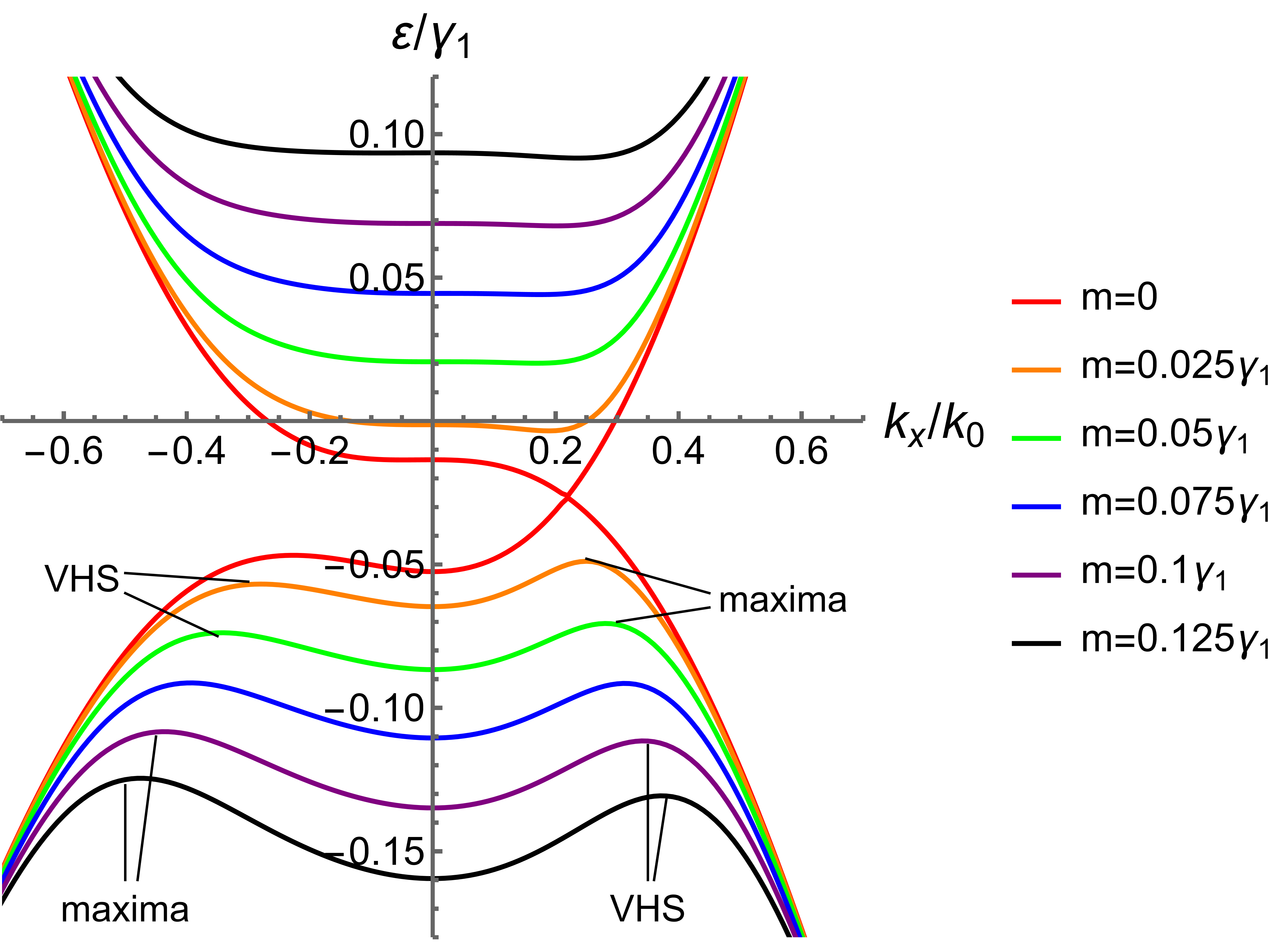
Figure S6: RTG surface bands at valley $K$ with different surface potentials $m$.

We first discuss interpretation 1. It requires that the hole density of a state in SC1 always coincides with that of the VHS singular point as $m$ varies. In Fig. S6, we plot the dispersion of the two surface bands with different surface potentials $m$ (parameters for band structure calculation are explained in Sec. S1). Focusing on the hole-doped side, we find the band maximum and the saddle-point VHS switch places at $m=0.075\gamma_{1}$ ($\sim 29$ meV, blue curve), which means the VHS corresponds to the valence band edge at $m=0.075\gamma_{1}$. As a result, at $m<0.075\gamma_{1}$, the VHS singular point shifts to lower hole densities as $m$ increases. In contrast, the experimentally observed SC1 shifts to higher hole densities as $m$ increases; therefore, for interpretation 1 to work, SC1 corresponds to $m$ values larger than $m=0.075\gamma_{1}$.

We choose $\Lambda_{K}$ to be the square area of $2.4k_{0}\times 2.4k_{0}$ at $K$ point, with a $100\times 100$ k-mesh to solve Eq. (S24) and (S27) numerically for the superconducting dome (i.e., the plot of the superconductor order parameter vs. electron density with fixed $U$). For attractive Hubbard interaction, the peak of the superconducting dome is exactly pinned at the singular point of the VHS since the density of states drives the superconducting transition. Then we obtain the superconducting dome plot for various surface potentials $m$ in Fig. S7(a). We find when the dome is peaked at $n_{e}=-1\times 10^{12}$ cm^-2, $m\approx 50$ meV$\equiv m_{o}$. This $m_{o}$ is determined by the band structure only, therefore, it agrees with Ref. [87] as expected (see Fig. 3 therein). To fit the transition temperature or $\Delta_{3\text{B}}$ to the order of magnitude $100$ mK, we must fine-tune the attractive interaction $U\sim 0.08\gamma_{1}=30$ meV.

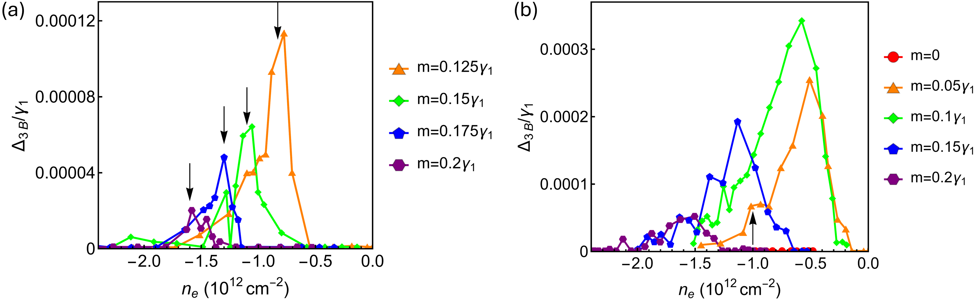
Figure S7: Two different interpretations of SC1 of the superconducting phase diagram of RTG. (a) SC1 corresponds to the peaks of the superconducting domes from an attractive Hubbard model (indicated by arrows), with $U=30$ meV. The onset surface potential (i.e., when the peak has electron density $-1\times 10^{12}$ cm^-2) is $m_{o}\sim 0.125\gamma_{1}\approx 50$ meV (orange curve). These peaks have a width of $0.1-0.2\times 10^{12}$ cm^-2. (b) SC1 corresponds to the left edge of the superconducting domes (indicated by an arrow for the orange curve only), with $U=42$ meV and $m_{o}\sim 0.05\gamma_{1}\approx 20$ meV. In both interpretations (a) and (b), the observed SC1 has the order parameter $\Delta_{3\text{B}}$ of the order of $0.0001\gamma_{1}$, giving a mean-field $T_{MF}\sim 100$ mK.

Next, we discuss interpretation 2 above. Since the attractive Hubbard model cannot describe other correlated states, one must assume that the numerically calculated superconducting dome has a much larger span in electron density than the experimentally observed one. In other words, phase SC1 only refers to the left edge of the dome calculated from the attractive Hubbard model, whereas the majority of the dome is replaced by other correlated states [50]. In Fig. S7(b), we show such a calculation that qualitatively reproduces the SC1 phase, for which we have to fine-tune $U\sim 0.11\gamma_{1}=42$ meV.

We note that the main difference between the two interpretations above lies in the conversion of the displacement field $D$ to the surface potential $m$. Using data from the bilayer graphene experiment [114] and taking into account the different thicknesses of the two materials, we estimate $m_{o}$ for SC1 to be 25-30 meV, which is closer to interpretation 2 above. Moreover, this estimated $m_{o}$ is close to the $m_{s}=0.06\gamma_{1}$ for the saturation of surface polarization in RTG, which suggests that the surface polarization effect plays an important role in the transition to SC1 as the displacement field increases.

IV.2 S4.2 Explanation of the effect of surface polarization on superconductivity

We use RTG as an example to explain the superconducting transition driven by the polarization of densities to some orbitals in a multi-orbital superconductor.

As mentioned in the main text, the linear combination form $\Delta_{v,\textbf{k}}=|\psi^{(v)}_{\textbf{k},1\text{A}}|^{2}\Delta_{1\text{A}}+|\psi^{(v)}_{\textbf{k},3\text{B}}|^{2}\Delta_{3\text{B}}$ for RTG implies that the set of two orders $\{\Delta_{1\text{A}},\Delta_{3\text{B}}\}$ contain more information than the order parameter in the band basis, $\Delta_{v,\textbf{k}}$. For instance, in a system where multiple order parameters $\alpha_{1}$, $\alpha_{2}$, … coexist, the ordering of another order parameter $\beta$, which is a linear combination of them ($\beta=\sum_{i}a_{i}\alpha_{i}$) may not tell us directly which order $\alpha_{i}$ leads to the transition.

One can diagonalize the BdG Hamiltonian Eq. (S36) analytically to obtain the zero-temperature gap equation in the orbital basis. In the case of RTG, the two orders $\Delta_{1\text{A}}$ and $\Delta_{3\text{B}}$ are coupled through the following two equations:

$$\begin{split}&\Delta_{1\text{A}}=\frac{U}{N_{c}}\sum_{\textbf{k}\in\Lambda_{K}}|\psi^{(v)}_{\textbf{k},1\text{A}}|^{2}\frac{\Delta_{v,\textbf{k}}}{\sqrt{\xi_{v,\textbf{k}}^{2}+\Delta_{v,\textbf{k}}^{2}}},\\ &\Delta_{3\text{B}}=\frac{U}{N_{c}}\sum_{\textbf{k}\in\Lambda_{K}}|\psi^{(v)}_{\textbf{k},3\text{B}}|^{2}\frac{\Delta_{v,\textbf{k}}}{\sqrt{\xi_{v,\textbf{k}}^{2}+\Delta_{v,\textbf{k}}^{2}}}.\end{split}$$ (S58)

The general solution is not simple, but the two limiting cases of zero polarization ($m=0$) and full polarization ($m\geqslant m_{s}$) can be analyzed easily. In the former case, $|\psi^{(v)}_{\textbf{k},1\text{A}}|^{2}=|\psi^{(v)}_{\textbf{k},3\text{B}}|^{2}=0.45$ near the VHS, and $\Delta_{1\text{A}}=\Delta_{3\text{B}}$, therefore we obtain a single equation involving $\Delta_{3\text{B}}$ only:

$$\Delta_{3\text{B}}=\frac{U}{N_{c}}\sum_{\textbf{k}\in\Lambda_{K}}0.45\frac{0.9\Delta_{3\text{B}}}{\sqrt{\xi_{v,\textbf{k}}^{2}+(0.9\Delta_{3\text{B}})^{2}}}.$$ (S59)

In the latter case, $|\psi^{(v)}_{\textbf{k},1\text{A}}|^{2}=0$, $|\psi^{(v)}_{\textbf{k},3\text{B}}|^{2}=0.9$ near the VHS, and $\Delta_{1\text{A}}=0$. Therefore the equation becomes

$$\Delta_{3\text{B}}=\frac{U}{N_{c}}\sum_{\textbf{k}\in\Lambda_{K}}0.9\frac{0.9\Delta_{3\text{B}}}{\sqrt{\xi_{v,\textbf{k}}^{2}+(0.9\Delta_{3\text{B}})^{2}}}.$$ (S60)

Assuming that $U$ does not change as $m$ varies (in reality, of course, it may renormalize), then comparing the two equations above, we find that the polarization to orbital 3B gives an additional factor of 2 to the coupling strength, even if the dispersion $\xi_{v,\textbf{k}}$ (i.e., the DOS) remains the same. The effects of the DOS enhancement and surface polarization are inseparable, but the factor 2 is still important for the superconducting transition as it is in the weak coupling limit and goes inside an exponential in the BCS-type solution of the self-consistency equation.

IV.3 S4.3 Superfluid weight calculation of SC1

Before calculating the superfluide weight, let us estimate the order of magnitude of different terms contributing to it for SC1. The conventional term $D_{s}^{\text{conv}}$ does not scale with $\Delta_{\alpha}$ if the coupling is weak and if $\mu$ measured from the band edge is much larger than $\Delta_{\alpha}$; the geometric term is always linear in the order parameter, so $D_{s}^{\text{geo}}\propto\Delta_{\alpha}$; whereas from Sec. S3.4 we know $D_{s}^{\Delta}\propto\Delta_{1\text{A}}\Delta_{N\text{B}}$. For SC1 of RTG, $\Delta_{1\text{A}}=0$ due to the polarization, so $D_{s}^{\Delta}=0$. Meanwhile, $\Delta_{3\text{B}}\sim 10^{-4}\gamma_{1}$ is the smallest energy scale in the system, making $D_{s}^{\text{geo}}\ll D_{s}^{\text{conv}}$.

In Fig. S8, we present the numerical calculation results for the superfluid weight $D_{s}$ of SC1 of RTG, at $m=0.06\gamma_{1}=23$ meV. Since the exact value of the order parameter may not be obtained from the transition temperature $T_{c}$ directly (there could be phase fluctuations), we calculate $D_{s}$ for a set of $\Delta_{3\text{B}}$ values of the order of $10^{-4}\gamma_{1}$. We also allow chemical potential $\mu$ to change around the VHS, including aligned with the singular point and the edge of it. It shows that $D_{s}$ does not scale with $\Delta_{3\text{B}}$, which means it is purely conventional. Even when $D_{s}$ depends on $\mu$, the ratio of $D_{s}/\Delta_{3\text{B}}$ is of the order of 100 (besides an additional factor of 54.9, see Sec. S3.2), regardless of the value of $\Delta_{3\text{B}}$ and $\mu$, indicating almost zero phase fluctuation in SC1 [110]. Therefore, the Berezinskii-Kosterlitz-Thouless transition temperature is the same as the mean-field critical temperature.

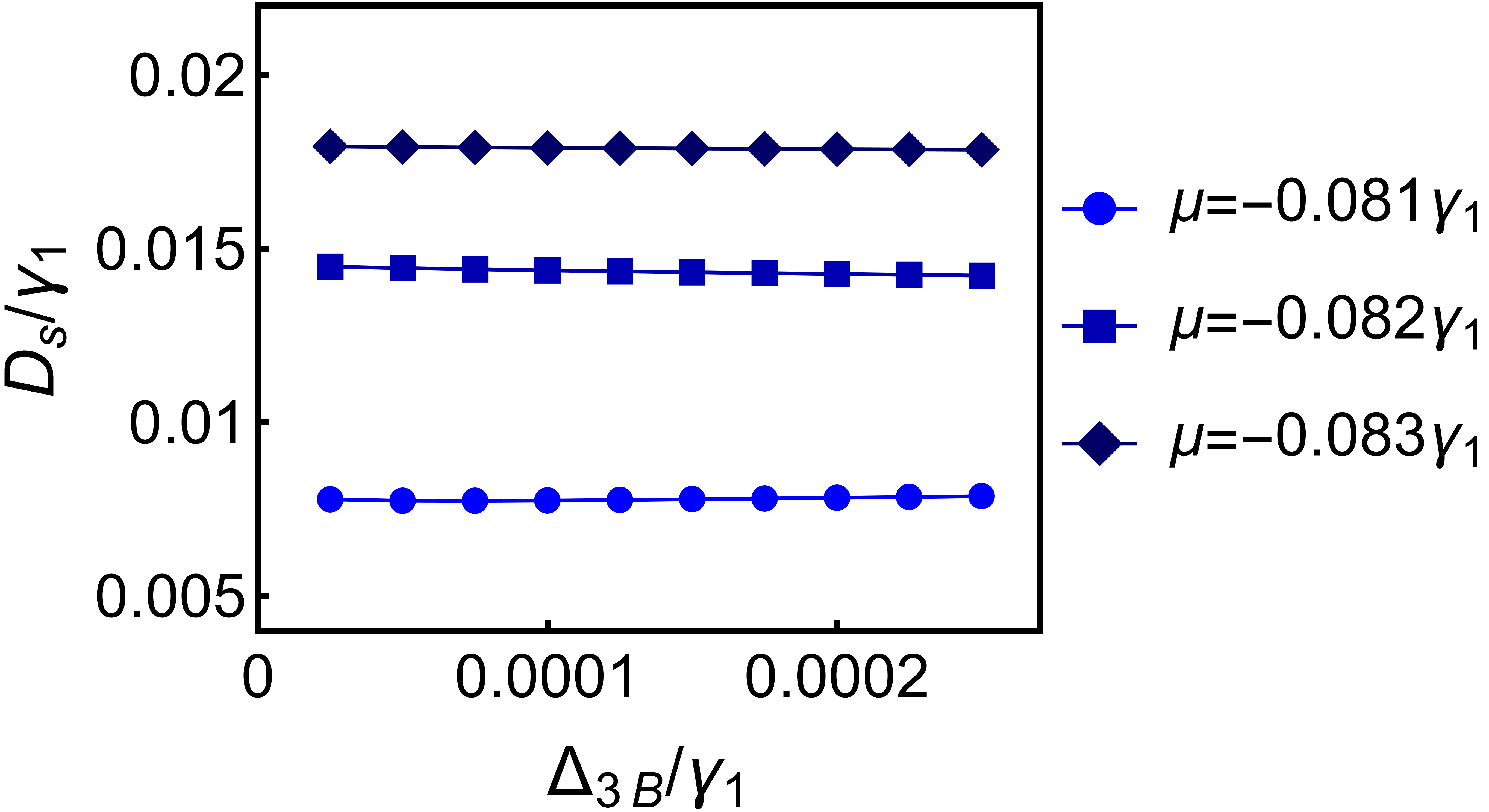
Figure S8: The total superfluid weight $D_{s}$ vs. $\Delta_{3\text{B}}$ at several chemical potentials $\mu$ close to the VHS, at surface potential $m=0.06\gamma_{1}$.