Constant Rate Isometric Embeddings of
Hamming Metric into Edit Metric

Abstract

A function $\varphi:\{0,1\}^{n}\to\{0,1\}^{N}$ is called an isometric embedding of the $n$-dimensional Hamming metric space to the $N$-dimensional edit metric space if, for all $x,y\in\{0,1\}^{n}$, the Hamming distance between $x$ and $y$ is equal to the edit distance between $\varphi(x)$ and $\varphi(y)$. The rate of such an embedding is defined as the ratio $n/N$.

It is well known in the literature how to construct isometric embeddings with a rate of $\Omega\left(\frac{1}{\log n}\right)$. However, achieving even near-isometric embeddings with a positive constant rate has remained elusive until now.

In this paper, we present an isometric embedding with a rate of $\frac{1}{8}$ by discovering connections to synchronization strings, which were studied in the context of insertion-deletion codes (Haeupler-Shahrasbi [JACM’21]). At a technical level, we introduce a framework for obtaining high-rate isometric embeddings using a novel object called misaligners. We speculate that, with sufficient computational resources, our framework could potentially yield isometric embeddings with a rate of $\frac{1}{5}$.

As an immediate consequence of our constant rate isometric embedding, we improve known conditional lower bounds for the closest pair problem and the discrete 1-center problem in the edit metric and NP-hardness of approximation results for clustering problems and the Steiner tree problem in the edit metric, but now with optimal dependency on the dimension.

We complement our results by showing that no isometric embedding $\varphi:\{0,1\}^{n}\to\{0,1\}^{N}$ can have rate greater than $\frac{15}{32}$ for all positive integers $n$. En route to proving this upper bound, we uncover fundamental structural properties necessary for every Hamming-to-edit isometric embedding. We also prove similar upper and lower bounds for embeddings over larger alphabets.

Finally, we consider embeddings $\varphi:\Sigma_{\text{in}}^{n}\to\Sigma_{\text{out}}^{N}$ between different input and output alphabets, where the rate is given by $\frac{n\log|\Sigma_{\text{in}}|}{N\log|\Sigma_{\text{out}}|}$. In this setting, we show that the rate can be made arbitrarily close to 1.

1 Introduction

Metric embeddings offer a powerful framework for formally comparing metric spaces by mapping points from a source space into a target space. The goal is to preserve pairwise distances faithfully (minimizing distortion), thereby revealing structural and computational properties associated with different notions of distance. These embeddings are particularly useful for understanding relationships between fundamental metrics, such as those central to coding theory, sequence analysis, and computational geometry.

Among the most fundamental distance measures, particularly in stringology and related fields, are the Hamming and the edit distances. The edit distance quantifies the minimum number of character insertions, deletions, and substitutions required to transform one string into another. Restricting these operations to only substitutions between equal-length strings yields the Hamming distance. Their distinct ways of capturing string similarity make both metrics pivotal in diverse areas, including pattern matching, machine learning, and computational biology [Nav01, LLL⁺16]. Consequently, numerous classical computational problems – like finding the closest pair of strings in a set [MV93, GXTL10] or identifying a representative center string for a dataset [WF74, NR05, LMW02] – are widely studied using these metrics, underpinning even public bioinformatics services [NCB].

Given the fundamental nature of both metrics, understanding their relationship via embedding is crucial. This paper systematically studies embeddings from the Hamming metric into the edit metric, exploring how the simpler substitution-only distance structure can be represented within the more general space allowing substitutions, insertions, and deletions. Formally, we investigate functions $\varphi:\{0,1\}^{n}\to\{0,1\}^{N}$, where the domain $\{0,1\}^{n}$ is equipped with the Hamming distance $\Delta_{\textnormal{{Hamming}}}$ and the codomain $\{0,1\}^{N}$ with the edit distance $\Delta_{\textnormal{{edit}}}$. We define the rate of the embedding $\varphi$ to be $\frac{n}{N}$. If $\varphi$ keeps distances unchanged except possibly multiplying all of them by some fixed constant, i.e., for some universal constant $K\geq 1$, we have $\Delta_{\textnormal{{edit}}}~(\varphi(x),~\varphi(y))=K~\cdot~\Delta_{\textnormal{{Hamming}}}(x,y)$, for all $x,y\in\{0,1\}^{n}$, then we call $\varphi$ a $1$-embedding. If $K=1$, i.e., $\varphi$ preserves distances exactly, then we call $\varphi$ an isometric embedding.

The goal of this work is to seek answers to fundamental questions about these embeddings: Is it possible to achieve a positive constant rate 1-embedding, or better an isometric embedding? What is the optimal rate achievable? Can we establish bounds on rates that are unattainable? Does using larger alphabets for isometric embeddings unlock the ability to obtain higher rates? By addressing all these questions, we provide a comprehensive study of embedding the Hamming metric into the edit metric.

1.1 Quest for Constant Rate 1-Embedding

In computational complexity, it is typically easier to prove the intractability of problems in the Hamming metric, and in such a situation, if we had a 1-embedding of the Hamming metric into the edit metric, then the hardness result would translate to the edit metric as well. These embeddings have been studied in the literature for exactly this purpose. For instance, a folklore embedding from the Hamming metric to the edit metric constructs the output string by inserting a uniformly random block of size $\Theta(\log n)$ after each character of the input string. This can be shown to result in an isometric embedding with high probability (and can be derandomized using constant relative distance codes in the edit metric such as the ones in [SZ99]).

However, this embedding achieves a rate of only $\frac{1}{\Theta(\log n)}$. Consequently, this implies that if a problem is hard for strings of length $n$ in the Hamming metric, then it remains hard in the edit metric, but only for strings of length $\Theta(n\log n)$. On the other hand, our intuition suggests that solving problems in the $n$-dimensional edit metric should be at least as hard as solving the same problems in the $n$-dimensional Hamming metric. The inability to provide a formal justification for this intuition leaves us wanting for a clearer understanding. To address this gap, we aim to answer the following natural question:

Does there exist a 1-embedding of the Hamming metric into the edit metric
with positive constant rate?

Our first result is an affirmative answer to the above question (in fact, we provide an isometric embedding). Our conceptual contribution in this regard is a clean connection between synchronization strings studied in the context of the study of codes for correcting insertion and deletion errors [HS21b, HSV18, HS18, HSS18, CHL⁺19] with the above question.

Theorem 1.1.

There exists a universal constant $C\geq 1$ such that for every positive integer $n$, there is an isometric embedding $\varphi_{n}:\{0,1\}^{n}\to\{0,1\}^{Cn}$ of the Hamming metric into the edit metric.

The use of synchronization strings to construct the above isometric embedding is elaborated further in Section 2.1. This result is quite surprising, as the best-known rate even for near-isometric embeddings was $\frac{1}{\Theta(\log n)}$ [Rub18].

As an immediate consequence of Theorem 1.1, we obtain the following meta theorem for discrete optimization problems in the edit metric. By discrete, we mean that the input is a set of points in the metric space, and the solution is some subset of the input points. For such problems, we have the following.

If a discrete optimization problem defined in the $n$-dimensional Hamming metric
cannot be solved in time $T(n)$ (for some computable function $T$),
then the same optimization problem defined in the $n$-dimensional Edit metric
cannot be solved in time $T(\Theta(n))$.

As concrete manifestations of this meta theorem, we prove optimal hardness results in two distinct settings. We remark that in the case of all the three theorems below, i.e., Theorems 1.2, 1.3, and 1.4, the previously known lower bounds or hardness results in the edit metric over binary strings was only for dimensions $d=O(\log n\cdot\log\log n)$, where the earlier mentioned embedding with rate $\Theta\left(\frac{1}{\log d}\right)$ was used. Thus, by reducing the dimension to $d=O(\log n)$ in the below three theorems, we obtain optimal dependency in the dimension.

Fine-Grained Complexity.

Using Theorem 1.1, we obtain conditional lower bounds for the closest pair problem and the 1-center problem in the edit metric with optimal dependency in the dimension.

Theorem 1.2.

Unless the Strong Exponential Time Hypothesis is false, for every $\delta>0$ there exists an $\varepsilon>0$ such that given as input sets $A,B\subseteq\{0,1\}^{d}$ of $N$ vectors (where $d=O_{\delta}(\log N)$), computing a $(1+\varepsilon)$-approximate closest pair in $A\times B$ in the edit metric requires time $\Omega(N^{2-\delta})$.

The above theorem follows immediately by combining Theorem 1.1 with the conditional lower bound for the bichromatic closest pair problem in the Hamming metric obtained by [Rub18]. Moreover, one can also obtain a conditional lower bound of $n^{1.5-o(1)}$ (with optimal dependency on dimension) against approximating the monochromatic closest pair problem in the edit metric by starting from [KM20]. Next, for the discrete 1-center problem, we have the following:

Theorem 1.3.

Unless the Hitting Set Conjecture is false, for every $\varepsilon>0$ there exists $c>1$ such that given as input a point-set $P\subseteq\{0,1\}^{d}$ where $|P|=N$ and $d=c\log N$, computing the point $x\in P$ that minimizes the maximum edit distance to all points in $P$ requires $\Omega(N^{2-\varepsilon})$ time.

The above theorem follows immediately by combining Theorem 1.1 with the conditional lower bound for the discrete 1-center problem in the Hamming metric obtained by [ABC⁺23].

NP Hardness.

Applying Theorem 1.1 to known NP-hardness of approximation results for discrete clustering problems [CKL22] and the discrete Steiner tree problem [FGK24] in the Hamming metric, we obtain below their hardness of approximation result in the edit metric with optimal dependency in the dimension.

Theorem 1.4.

It is NP-hard to approximate:

• the discrete $k$-means problem (resp. discrete $k$-center problem and discrete $k$-median problem) on $N$ points in the $\{0,1\}^{O(\log N)}$ dimensional edit metric to a factor better than $1.38$ (resp. $3-o(1)$ and $1.12$).

• the discrete Steiner tree problem on $N$ terminals in the $\{0,1\}^{O(\log N)}$ dimensional edit metric to a factor better than $1.004$.

1.2 High Rate Isometric Embedding

Theorem 1.1 directly implies that good Hamming codes (those with positive constant rate and relative distance) yield corresponding codes in the edit metric. Since the isometric embedding given by the theorem simply uses padding, these embedded codes preserve many structural properties of their Hamming counterparts. The drawback, however, is that the embedding reduces the code’s rate and relative distance by the constant factor $C$ introduced in the theorem statement. This motivates the following question:

What is the optimal rate for an isometric embedding
of the Hamming metric into the Edit metric?

We note that this question is also of pure combinatorial interest. Consider the weighted complete graph $\widetilde{Q}_{n}$ (resp. $\widetilde{A}_{N}$) on the vertex set $\{0,1\}^{n}$ (resp. $\{0,1\}^{N}$) where the weight of the edge on any two vertices corresponds to their Hamming distance (resp. edit distance). It is clear that for every pair of vertices, their weight in $\widetilde{A}_{n}$ is at most their weight in $\widetilde{Q}_{n}$. A natural question then arises: what is the smallest $N>n$, such that we can identify an isomorphic copy of $\widetilde{Q}_{n}$ in $\widetilde{A}_{N}$?

To make progress on this question, we introduce objects called misaligners, which can be thought of as codes in the edit metric with robust distance guarantees, in two distinct ways. First, misaligner codewords contain wildcard symbols and, irrespective of how these wildcards are instantiated, a large pairwise distance is guaranteed between any two distinct codewords. The second guarantee is even stronger: not only is the distance between pairs of codewords large, but the distance also remains large even when comparing a codeword with a concatenation of multiple codewords. This protects against situations where the concatenation of the suffix and prefix of two codewords might closely resemble another codeword. Formally defining misaligners requires a bit of work, but below, when we speak of $(\alpha,m)$-misaligners, we informally refer to misaligners that have codewords of length $m$ and relative distance $\alpha$. We elaborate more on the parameters of misaligners in Section 2.2, and it is formally defined in Definition 4.1.

In addition to misaligners, we also explicitly formulate objects called $\varepsilon$-locally self-matching strings, which are strings in which every substring of length $\ell$ has non-vertical matches of size at most $\varepsilon\ell$, where, by non-vertical matches, we forbid matching an index to itself. These objects appear implicitly in the context of synchronization strings introduced by Haeupler and Shahrasbi [HS21b]. Again, we elaborate more on this notion in Section 2.2, and it is formally defined in Definition 5.1.

One of our main technical contributions is showing how to utilize the construction of misaligners and locally self-matching strings to design high-rate isometric embeddings of the Hamming metric into the edit metric.

Theorem 1.5 (Informal statement of Theorem 6.1).

Suppose for some $\varepsilon,\alpha>0$ and some integer $m$, there exists an $(\alpha,m)$-misaligner and a $\varepsilon$-locally self-matching string, then for every positive integer $n$ there is an isometric embedding $\varphi_{n}:\{0,1\}^{n}\to\{0,1\}^{Rn}$ of the Hamming metric into the edit metric, where:

$$R=\left\lceil\frac{1}{(1-\varepsilon)\alpha-\frac{1}{3m-1}}\right\rceil.$$

Even with limited computing resources, we were able to construct a $(0.1625,320)$-misaligner and a $0.224$-locally self-matching string. This yields the following embedding (see Section 8 for more details).

Corollary 1.6.

For every positive integer $n$, there is an isometric embedding $\varphi_{n}:\{0,1\}^{n}\to\{0,1\}^{8n}$ of the Hamming metric into the edit metric.

It is possible that with sufficient time and computing resources (i.e., by making $m$ large and $\varepsilon$ tiny), we can use Theorem 1.5 to obtain embeddings with rate approaching $\alpha$, where $\alpha$ is the relative distance parameter of the misaligner. From the current computer search, we speculate that $\alpha$ is above 0.2. Thus, it is possible in the future that we have an isometric embedding where $n$ bits are mapped only to $5n$ bits.

As remarked earlier, locally self-matching strings are closely related to synchronization strings [HS21b]. Both these objects are constructed using the algorithmic Lovasz Local Lemma [MT10]. Prior work established that for all positive integers $n$ there exists a $\varepsilon$-locally self-matching string $w$ of length $n$ over alphabet of size $O(1/\varepsilon^{2})$ [CHL⁺19]. However, we could not use any of the existing analyses using the Lovasz Local Lemma in the synchronization strings literature due to the large hidden constants in those works. Thus, en route to proving Corollary 1.6, we also improve the analysis of constructing synchronization strings. To the best of our knowledge, prior to our work, the hidden constant in the alphabet size bound in these analyses was about $4900\cdot e^{2}\approx 3.6\times 10^{4}$, and we have reduced to it a quantity that approaches $e^{2}\approx 7.39$ as $\varepsilon$ goes to 0.

Theorem 1.7.

Let $\Sigma$ be a finite set and $\varepsilon\in\left(0,\frac{1}{2}\right]$ such that the following holds:

$$|\Sigma|\geq\frac{e^{2}}{\varepsilon^{2}}\cdot\left(1+4\sqrt[4]{\varepsilon}\right).$$

Then, for all positive integers $n$, there exists a $\varepsilon$-locally self-matching string $w$ over $\Sigma$ of length $n$.

As an immediate consequence of this improved analysis, we also obtain the following (proved in Appendix B).

Corollary 1.8.

There exists an infinite $0.999606$-synchronization string over an alphabet of size four.

The above result adds to the work of [CHL⁺19] where it was shown that there is some unspecified constant $\varepsilon$ such that $\varepsilon$-synchronization strings exist over alphabet four.

1.3 Structure of Isometric Embeddings and Impossibility Results

The embedding in Theorem 1.5 is an example of an interleaved embedding, where the output string is formed by interleaving the input bits with sequences of bit strings that do not depend on the input. A natural question is whether there exist isometric embeddings, potentially with better rates, that do not follow this interleaving framework. We answer this negatively, demonstrating that isometry necessitates an interleaved structure in the output strings.

Theorem 1.9 (Isometry implies Interleaving).

Every isometric embedding $\varphi:\{0,1\}^{n}\to\{0,1\}^{N}$ of the Hamming metric into the edit metric must be an interleaved embedding.

A precise formulation of Theorem 1.9 requires a formal definition of interleaved embeddings, which we provide in Section 10. Informally, we naturally extend the intuitive notion of interleaving input bits with fixed bit patterns by allowing two additional flexibilities. First, we allow the input bits to appear out-of-order — e.g., the second input bit might appear after the first input bit in the output string. We further allow some of the input bits to appear complemented in the output string. Thus, an isometric embedding of the Hamming metric into the edit metric is completely determined by three components — the order in which input bits appear in the output, the subset of input bits that are flipped, and the sequence of fixed bit strings that are to be interleaved with the input bits.

This structural constraint on Hamming-to-edit isometric embeddings enables us to derive bounds on the achievable rate. In particular, we show that for binary strings, any isometric embedding must stretch the input strings by a factor greater than 2.133.

Theorem 1.10.

There exists a positive integer $n_{0}$ such that every isometric embedding $\varphi:\Sigma^{n}\to\Sigma^{N}$ of the Hamming metric into the edit metric with $n\geq n_{0}$ must have rate at most $\frac{15}{32}$.

We further generalize these results to larger alphabets, by extending the definition of interleaved embeddings to larger alphabets (see Section 10.1), proving that every isometric embedding must be an interleaved embedding, and then showing an analogous statement to Theorem 1.10.

Theorem 1.11.

For every alphabet $\Sigma$, there exists an integer $n_{0}$ such that every isometric embedding $\varphi:\Sigma^{n}\to\Sigma^{N}$ of the Hamming metric into the edit metric with $n\geq n_{0}$ must have rate at most $\frac{1}{2}-\frac{1}{16|\Sigma|}$.

1.4 Isometric Embeddings over Larger Alphabets and Surpassing the $\nicefrac{{1}}{{2}}$ Rate Barrier

Having established the rate limitations for isometric embeddings over the binary alphabet, we next explore if leveraging a larger alphabet $\Sigma$ enables the construction of embeddings $\varphi:\Sigma^{n}\to\Sigma^{N}$ with potentially improved rates. As in the binary case, we can obtain high-rate embeddings over $\Sigma$ by using misaligners for larger alphabets. In fact, it is not hard to see that misaligners designed for the binary alphabet also function as misaligners for larger alphabets, without any loss in parameters. Therefore, increasing the alphabet size can only improve the achievable rate.

We show that even without relying on the full machinery of misaligners, one can obtain isometric embeddings with rates arbitrarily close to $\frac{1}{3}$ by making the alphabet large enough.

Theorem 1.12.

For any $\rho>0$, there exists an alphabet $\Sigma$ such that for every positive integer $n$, there is an isometric embedding $\varphi_{n}:\Sigma^{n}\to\Sigma^{N}$ of the Hamming metric into the edit metric with rate at least $\frac{1}{3}-\rho$.

Theorem 1.11 tells us that as long as the input and output alphabets remain the same, the rate in Theorem 1.12 can never be improved to $\frac{1}{2}$ or anything better. But what if we allow the input and output alphabets to be different?

In this setting, our notion of rate needs to be refined. In particular, when using the larger output alphabet, the appropriate measure to consider is not the lengths of strings but the number of bits contained in them. Thus, for an embedding $\varphi:\Sigma_{\textnormal{in}}\to\Sigma_{\textnormal{out}}$, we define the rate as $\frac{n\log|\Sigma_{\textnormal{in}}|}{N\log|\Sigma_{\textnormal{out}}|}$. With this refined definition, we show that not only can the $\frac{1}{2}$ rate barrier be surpassed, but the rate can actually be made arbitrarily close to 1!

Theorem 1.13.

For every $\rho>0$, there exist alphabets $\Sigma_{\textnormal{in}}$, $\Sigma_{\textnormal{out}}$ such that for all positive integers $n$, there is an isometric embedding $\varphi_{n}:\Sigma_{\textnormal{in}}^{n}\to\Sigma_{\textnormal{out}}^{N}$ of the Hamming metric into the edit metric with rate at least $1-\rho$.

We provide a proof of Theorem 1.13 in Section 12 while Theorem 1.12 is proven in Section 9.

1.5 Related works

In this subsection, we survey two lines of related works.

Embedding Edit metric to Hamming metric.

Embeddings in the other direction, i.e., from the edit metric to the Hamming metric, are abundant in the literature. A key motivation for embedding the edit metric into the Hamming metric is computational: Hamming distance can be computed efficiently in linear time, whereas edit distance cannot be solved in sub-quadratic time unless the Strong Exponential Time Hypothesis is false [BI18]. This underscores the need for approximation algorithms that can run in subquadratic time. One potential approach is to develop an embedding with low distortion, where the embedding process itself can be performed in subquadratic time.

The seminal work by Ostrovsky and Rabani [OR07] shows an embedding of the edit metric into the Hamming metric with distortion $2^{O(\sqrt{\log n\log\log n})}$. The rate achieved is $1/\log n$, and the embedding can be computed in polynomial time. There has been extensive research aimed at establishing lower bounds for the distortion of any such embedding, with the best-known lower bound being $O(\log n)$ [KR09].

An alternative approach to potentially improve the results above is through randomized embeddings. In this approach, the embedding function takes both an input string and a random string, and we measure the distortion when two strings are mapped using the same random string sequence. Within this framework, Johwari [Jow12] showed the existence of $O\left(\log n\log^{*}n\right)$-distortion. Subsequently,  [CGK16] were the first to eliminate the dependence of the dimension in the distortion, achieving a quadratic distortion, i.e., if the edit distance between the input strings is at most $k$, then the Hamming distance between the embedded strings is bounded by $O(k^{2})$.

Synchronization strings.

Synchronization strings were introduced by Haeupler and Shahrasbi [HS21b] in the context of codes able to tolerate insertion and deletion errors. In our context, the original application of synchronization strings can be viewed as embedding the Hamming metric near isometrically into the edit metric by increasing the alphabet size by a constant factor. Throughout the years, these strings have found uses in many settings, including interactive coding [HSV18], locally decodable insertion-deletion codes [HS18], and list decodable insertion-deletion codes [HSS18]. For a survey of the many uses of synchronization strings and how they are constructed, the reader is referred to [HS21a].

1.6 Organization of Paper

In Section 2, we provide an overview of the proofs for our main results. In Section 3, we introduce some notations and definitions of relevance to this paper. In Section 4, we formally define misaligners – the key ingredient to our high-rate isometric embeddings. In Section 5, we introduce locally self-matching strings and give improved bounds on alphabet size for such strings. In Sections 6 and 7, we show how to combine misaligners and locally self-matching strings to obtain high-rate isometric embeddings for binary strings. In Section 8, we describe how to find a misaligner using computer search and give an explicit rate $\frac{1}{8}$ isometric embedding for binary strings proving Corollary 1.6. In Section 9, we consider embeddings over larger alphabets and prove Theorem 1.12. Then Section 10 is dedicated to defining interleaved embeddings and proving Theorem 1.9. In Section 11, we derive rate upper bounds for isometric embeddings proving Theorem 1.11. Finally, in Section 12, we show how to surpass the $\frac{1}{2}$ rate barrier by considering different-sized input and output alphabets and prove Theorem 1.13.

2 Proof Overview

In Section 2.1, we provide a proof overview of Theorem 1.1 which is our main conceptual contribution. We do not provide a formal proof of Theorem 1.1 as it is subsumed by Theorem 1.5 and Corollary 1.6. In Section 2.2, we provide a proof overview of Theorem 1.5, which is one of our main technical contributions. Furthermore, in Section 2.3, we summarize the key ideas behind our proof of Theorem 1.9, while in Section 2.4, we provide a proof sketch of Theorem 1.11.

2.1 Constant Rate Embeddings via Synchronization Strings

Our first observation is that if we are allowed an unbounded output alphabet, then there is a straightforward isometric embedding that takes any input string and interleaves it with a string with all distinct symbols. This embedding is clearly isometric since any misalignment of these new symbols results in mismatches, increasing the edit cost beyond the simple identity alignment, which corresponds to the Hamming distance between the input strings. Moreover, the length of the output strings produced by this embedding is only twice that of the input strings.

However, our goal is to have a binary output alphabet, not an unbounded one. So, as an intermediate step, let us limit ourselves to a large but constant-sized output alphabet. Now, if we want to mimic our earlier embedding, we would need to find a string over a constant-sized alphabet that approximates the string with all distinct symbols. It turns out that objects known as synchronization strings [HS21b] have the exact property that we want. Synchronization strings have many equivalent definitions. The one that is useful for our discussion is the following — a string is said to be an $\varepsilon$-synchronization string if, for every substring, its relative self-edit distance is at least $1-\varepsilon$. For every value of $\varepsilon$, one can efficiently construct $\varepsilon$-synchronization strings over an alphabet of size $\Theta(1/\varepsilon^{2})$ [CHL⁺19]. We now illustrate how these strings can be used to construct constant-rate isometric embeddings over a larger but fixed-size output alphabet.

To embed a string of length $n$, consider a $\nicefrac{{2}}{{3}}$-synchronization string of length $3n$ over an alphabet $\Sigma$ that is disjoint from the input alphabet $\{0,1\}$. The embedding process, applied to an input string of length $n$, involves inserting $3$ symbols from the synchronization string after every input symbol. It is evident that both the rate and the output alphabet size remain constant.

Let us briefly explain why this gives an isometric embedding. Suppose it does not; then there must be a pair of strings such that the edit distance between their embeddings is strictly smaller than their Hamming distance. Consider an optimal edit alignment for converting the embedded strings. It can be shown that this alignment partitions the strings into intervals, where for each interval in the partition, either the entire interval is mapped using the identity mapping or it is self-aligned such that none of its characters are mapped to themselves. See Figure 1 for the partitions of the alignment.

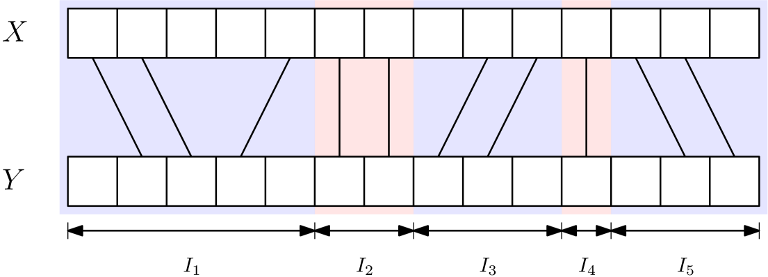
Figure 1: An optimal alignment converting the embedded string $X$ to the embedded string $Y$. Note the alternating maximal nowhere-vertical and vertical intervals (highlighted blue and red, respectively) $I_{1},I_{2},I_{3},I_{4}$ and $I_{5}$.

If the edit distance is indeed strictly less than the Hamming distance, then there is at least one interval, say of length $\ell$, in this partition where none of its characters are mapped to themselves, but the edit cost in that interval is strictly less than the Hamming cost, which is at most $\nicefrac{{\ell}}{{4}}$. We then show that this implies the existence of a substring in the synchronization string with a relative self-edit distance less than $\nicefrac{{1}}{{3}}$, which is a contradiction. This substring can be found by considering the aforementioned interval and deleting all the characters that come from the input strings. This results in a substring with length $\ell^{\prime}:=\nicefrac{{3\ell}}{{4}}$. One can also find a self-alignment of this substring by taking the original alignment, keeping it unchanged except for positions where some character in the substring was matched to some character in one of the input strings. In those positions, we simply apply a deletion. It is not hard to see that the cost of this alignment remains unchanged and is thus less than $\nicefrac{{\ell}}{{4}}=\nicefrac{{\ell^{\prime}}}{{3}}$, which contradicts the fact that the string used to pad is a $\nicefrac{{2}}{{3}}$-synchronization string. In Figure 2, the red characters are part of some $\varepsilon$-synchronization string, and the green ones are part of some input string.

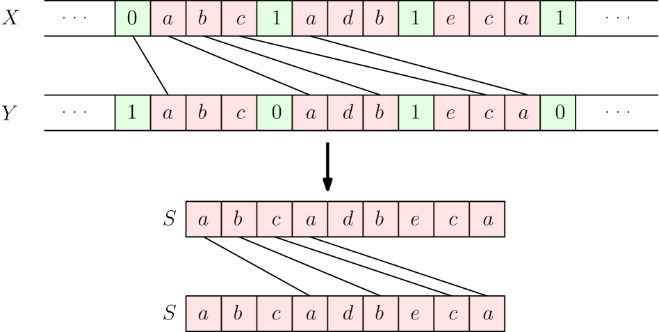
Figure 2: A nowhere-vertical alignment on some interval in the embedded strings $X$ and $Y$ implies a self-alignment of a substring $S$ of the $\varepsilon$-synchronization string with the same cost.

One can then bring the output alphabet size down to two using the following alphabet reduction procedure — we replace each character of the synchronization string with its binary encoding (of length $\log|\Sigma|$) along with an opening and closing block of $0$s and $1$s with lengths equal to that of the binary encoding. The final resulting rate is still constant. However, the large alphabet sizes required to construct $\varepsilon$-synchronization strings means that the resulting rate is far from optimal. With the specific setting of $\varepsilon=\nicefrac{{2}}{{3}}$ and known bounds for alphabet sizes for synchronization strings, one gets a rate of about $\nicefrac{{1}}{{153}}$ from this.

2.2 Optimizing the Rate: Enter Misaligners!

To improve the rate of our embedding, we move away from the framework of interleaving a synchronization string over a larger alphabet and then performing an alphabet reduction. Instead, we utilize a tailored construction that gives us a much larger rate.

The key ingredient in our construction is an object called a misaligner, which the reader should think of as a code in the edit metric with robust distance guarantees. A misaligner consists of a set of fixed-length codewords over the alphabet $\{0,1,\star\}$, where $\star$ is a special wildcard symbol. Each codeword contains a wildcard symbol at every $t^{\text{th}}$ position, where $t$ is a parameter that controls the rate of the embedding. Thus, if one concatenates a sequence of codewords from the misaligner, one obtains a long binary string with wildcard symbols at every $t^{\text{th}}$ position. To embed some input string, one simply substitutes these wildcard symbols with symbols from the input string. The rate of this embedding is $\nicefrac{{1}}{{t}}$ by definition.

To fully describe the embedding, one also needs to specify the order in which codewords from the misaligner are concatenated. To do this, we make use of a variant of synchronization strings, which we call locally self-matching strings. Given $\varepsilon\in(0,1)$, an $\varepsilon$-locally self-matching string is one where every substring has at most an $\varepsilon$-fraction of matches to itself if one is not allowed to match vertically. The embedding procedure is now clear: to embed an input string, we first start with a sufficiently long locally self-matching string over some large alphabet. Next, we replace each symbol of this string with a codeword from the misaligner. Note that in order to do this, the number of codewords in the misaligner must be at least as large as the alphabet of the locally self-matching string. Finally, we substitute the wildcard symbols in this string with symbols of the input string to obtain the embedded string. Our goal is to show that by choosing $t$ sufficiently large, the properties of the locally self-matching string and the misaligner guarantee that the resulting construction is an isometric embedding.

For concreteness, in the remainder of this section, let us assume that a 0.1-locally self-matching string $s$ exists over some large alphabet $\Sigma$. We also assume that a misaligner $\mathcal{C}$ with $|\Sigma|$ many codewords exists. The other properties of this misaligner will be specified later. We will show how the properties of $s$ and $\mathcal{C}$ will guarantee isometry.

Let us call a codeword with its wildcard symbols instantiated a block. Assume for the sake of contradiction that the embedding we just described is not an isometric embedding. As before, this implies the existence of an interval with an edit cost that is strictly lower than its Hamming cost. The first guarantee that the misaligner provides is that this interval must contain at least two full blocks. This is ensured by enforcing the codewords of the misaligner to have the following property — for any substring arising from the concatenation of multiple codewords and not containing two full blocks must have the edit distance equal to the Hamming distance no matter how the wildcard symbols are instantiated. See Figure 3 for an illustration of this property.

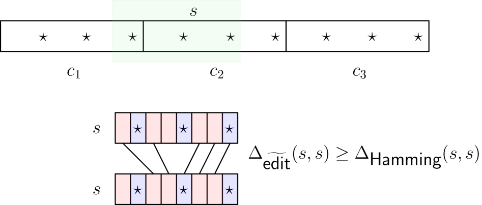
Figure 3: For short intervals, the misaligner guarantees isometry: any nowhere-vertical edit alignment must pay at least as much as the Hamming distance, no matter how the wildcards are instantiated.

For larger intervals (i.e., intervals containing at least two full blocks), we assume for simplicity that the interval consists solely of a sequence of full blocks with no partial blocks at the boundaries. The analysis then goes on to assess the cost of the optimal alignment by decomposing it into contributions from individual blocks. Our objective is to demonstrate that, for most blocks, there is a substantial cost, which, for the purposes of this discussion, is 0.2 times the length of a block.

Our first observation concerns any two blocks within the specified interval that are instantiations of the same codeword but appear at different positions in the embedded strings. Without loss of generality, we note that in an optimal alignment between these embedded strings, exactly one of the following cases occurs: either all of the characters of the first block are matched “vertically” to all of the characters in the second block in the optimal alignment (in which case, the first block is referred to as “bad”; see Figure 4), or none of the characters are matched “vertically”. From the set of bad blocks and their matches, one can recover a sequence of nowhere-vertical matches in the original locally self-matching string $s$. Since $s$ was a 0.1-locally self-matching string, one can thus conclude that the fraction of bad blocks is at most 0.1.

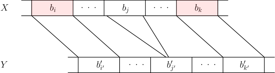
Figure 4: The blocks $b_{i}$ and $b^{\prime}_{i^{\prime}}$ as well as $b_{j}$ and $b^{\prime}_{j^{\prime}}$ and $b_{k}$ and $b^{\prime}_{k^{\prime}}$ are instantiations of the same codeword and appear in different positions in $X$ and $Y$. The bad blocks — those where all characters are matched vertically — are highlighted in red.

Next, let us analyze the remaining blocks. The optimal alignment transforms each of these blocks into a substring coming from the concatenation of multiple blocks. If the size of this substring exceeds $0.2$ times the block size, then the cost will also exceed $0.2$. For the remaining blocks, the misaligner must ensure that the edit cost of each block remains substantial. This can be accomplished by satisfying the following requirements:

Consider a block $b$ and take any substring $s$ of roughly the same size, composed of partial blocks. If none of these blocks is equal to $b$, we require that the relative edit cost between $b$ and $s$ is at least $0.2$. If one of these blocks is equal to $b$, we require that the edit cost of alignments with no vertical edges between $b$ and its counterpart in $s$ is at least $0.2$. See Figure 5 for an illustration.

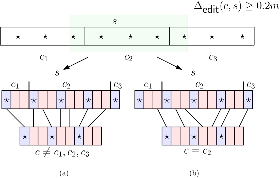
Figure 5: The alignment transforms every block $c$ into a substring $s$ arising from the concatenation of multiple blocks. If $c$ and $s$ are roughly the same size, the misaligner guarantees the relative edit distance between $c$ and $s$ is at least 0.2. Observe that in case (b), the alignment has no vertical edges between $b$ and its counterpart in $s$.

Since bad blocks cost zero, the total cost is given by the sum of costs incurred by the non-bad blocks. Thus, by the properties of the misaligner and the locally self-matching string, the relative cost is lower bounded by $(1-0.1)\times 0.2=0.18$. Therefore, if we choose $t=6$, we arrive at a contradiction, as the cost would then exceed the number of wildcards, which is an upper bound on the Hamming distance in the interval between any two strings. Consequently, we can achieve a $\nicefrac{{1}}{{6}}$-rate isometric embedding. The case where the interval may contain partial blocks introduces additional requirements, which are detailed in Section 4.

2.3 Unveiling the Interleaved Structure of Isometric Embeddings

In this section, we outline the key ideas behind our proof of Theorem 1.9, which states that every isometric embedding of the Hamming metric into the edit metric is necessarily an interleaved embedding. The formal definition of interleaved embeddings is deferred to Section 10. Here, we instead fix an arbitrary isometric embedding $\varphi:\{0,1\}^{n}\to\{0,1\}^{N}$ and make a series of observations that reveal certain constraints on $\varphi$, ultimately uncovering its interleaved nature.

We start by fixing an input string $x\in\{0,1\}^{n}$ and ask what happens to $\varphi(x)$ as we flip a single bit in $x$. Since $\varphi$ is isometric, flipping a single bit in $x$ must correspond to exactly one bit flip in $\varphi(x)$. This allows us to define a function $\eta_{x}:[n]\to[N]$, $\eta_{x}(i)$ is the unique index in $\varphi(x)$ that is flipped if the $i^{\text{th}}$ bit of $x$ is flipped.

Next, we show that the function $\eta_{x}$ is injective, meaning that different bit flips in $x$ affect different positions in the output $\varphi(x)$. This is not hard to see — if two different bit-flips in $x$ affected the same position in $\varphi(x)$, then we would obtain a pair of strings at Hamming distance 2 whose images under $\varphi$ have edit distance 0, contradicting the fact that $\varphi$ is isometric.

A crucial step in the proof is showing that $\eta_{x}(i)$ does not depend on $x$. That is, once $i$ is fixed, flipping the $i^{\text{th}}$ bit in any input string always affects the same location in the output. This means the function $\eta_{x}$ is the same for all inputs and can simply be written as $\eta$. This can be proven by fixing a pair of input strings $x,y$ and an index $i$ and inducting on the Hamming distance between $x$ and $y$. This key step is presented in detail in Section 10.

Finally, we show that $\varphi(x)[\eta(i)]$ depends only on $x[i]$, meaning that each input bit is mapped consistently to the same output position, either preserving or flipping its value. With this, the interleaved nature of $\varphi$ is revealed: the output positions fall into two categories — those that directly correspond to input bits (determined by $\eta$) and the remaining positions that are independent of the input. For the full details, we refer to Section 10.

2.4 Upper Bounds on the Rate

In this section, we outline the proof of Theorem 1.11, which establishes that any isometric embedding of the Hamming metric into the edit metric must have a rate strictly bounded away from $\frac{1}{2}$. More precisely, we aim to show that for any alphabet $\Sigma$, there exists some $\varepsilon>0$ such that for sufficiently large $n$, no isometric embedding $\varphi:\Sigma^{n}\to\Sigma^{N}$ can achieve a rate exceeding $\frac{1}{2}-\varepsilon$.

Our approach is by contradiction: we assume that for all $n$, there exists an isometric embedding $\varphi$ with a rate exceeding the claimed bound. The goal then is to show that as $n$ grows, $\varphi$ cannot remain isometric. Specifically, we seek a pair of strings such that the edit distance between their embeddings is strictly smaller than their Hamming distance, contradicting isometry. Rather than constructing such a pair explicitly, we will argue its existence via the probabilistic method.

The key idea is to consider a collection $\mathcal{C}$ of carefully chosen triples $(x,y,\mathcal{A})$, where $x,y\in\Sigma^{n}$ and $\mathcal{A}$ is an edit distance alignment between $\varphi(x)$ and $\varphi(y)$. We then select a random triple from $\mathcal{C}$ and show that the expected cost of $\mathcal{A}$ with respect to the embeddings $\varphi(x)$ and $\varphi(y)$ is too low, ensuring the existence of a triple in $\mathcal{C}$ that violates the isometry of $\varphi$.

Description of $\mathcal{C}$.

The alignments in $\mathcal{C}$ are simple “shift” alignments, where each symbol in one string is matched with a symbol in the other string shifted by a fixed amount. More formally, for a non-zero integer $\delta$, we define $\mathcal{A}_{\delta}$ as the alignment where each symbol in the first string is paired with a symbol in the second string shifted by $\delta$ positions. We consider alignments of the form $\mathcal{A}_{\delta}$ where $|\delta|$ is bounded by a constant that depends on the rate we seek to rule out, in particular, $\varepsilon$, but is independent of $n$.

Since $\varphi$ is isometric, by the generalization of Theorem 1.9 to larger alphabets (i.e., Theorem 10.9), it must be an interleaved embedding. This implies that some symbols in $\varphi(x)$ are “frozen” (independent of $x$), while the remaining symbols are “mutable” (determined by $x$). Using this observation, for each alignment $\mathcal{A}_{\delta}$, we construct a pair of strings $x_{\delta},y_{\delta}\in\Sigma^{n}$ satisfying the following two properties.

• The Hamming distance between $x_{\delta}$ and $y_{\delta}$ is $n$.

• No mutable symbol in $\varphi(x_{\delta})$ is substituted under $\mathcal{A}_{\delta}$; they are either matched or deleted.

Section 11 details how to construct such pairs given $\mathcal{A}_{\delta}$. The final collection $\mathcal{C}$ consists of all triples $(x_{\delta},y_{\delta},\mathcal{A}_{\delta})$ for $\delta$ in a constant-sized set of shifts.

Bounding the Expected Alignment Cost.

We now pick a random $(x_{\delta},y_{\delta},\mathcal{A}_{\delta})$ from $\mathcal{C}$ and analyze the expected cost of $\mathcal{A}_{\delta}$ with respect to $\varphi(x_{\delta})$ and $\varphi(y_{\delta})$. Since $\mathcal{A}_{\delta}$ is a shift alignment, its cost due to insertions and deletions is at most a constant. Moreover, by our choice of $x_{\delta}$ and $y_{\delta}$, there are no substitutions involving mutable symbols — only frozen symbols contribute to substitutions. Now if the rate of $\varphi$ is too high, the number of frozen symbols must be small, which in turn means the expected number of substitutions is also small. We show that for sufficiently large $n$, the expected cost of $\mathcal{A}_{\delta}$ falls below $n$, leading to a contradiction. For the detailed calculations along with choices for the maximum value of $\delta$, the reader is referred to Section 11.

3 Preliminaries

Intervals and Strings.

For any positive integer $n$, we define $[n]:=\{1,2,\ldots,n\}$. For positive integers $i,j$, we define the interval $[i,j]:=\{i,i+1,\ldots,j\}$. We define a partial order on the set of all intervals in the following natural way — given intervals $I=[i,j]$ and $I^{\prime}=[i^{\prime},j^{\prime}]$, we say $I<I^{\prime}$ if and only if $j<i^{\prime}$.

A string $x=x[1]x[2]\cdots x[n]$ over alphabet $\Sigma$ is a sequence of $n$ symbols from $\Sigma$. We denote by $|x|$ the length of the string $x$. Given a string $x$ and an interval $I=[i,j]\subseteq[|x|]$, we denote by $x_{|I}$ the substring $x[i]x[i+1]\cdots x[j-1]x[j]$. We further extend this notation to arbitrary sets of indices and not just intervals. Given any subset $S=\{i_{1},i_{2},\ldots,i_{k}\}$ with $1\leq i_{1}<i_{2}<\cdots<i_{k}\leq|x|$, we denote by $x_{|S}$ the string $x[i_{1}]x[i_{2}]\cdots x[i_{k}]$. We denote by $x^{\mathcal{R}}$ the reverse of the string $x$.

Edit distance alignments.

Let $x,y\in\{0,1\}^{*}$ be two strings of length $n$ and $m$, respectively, such that $n\geq m$. An edit distance alignment between $x$ and $y$ is a set $\mathcal{A}=\{(i_{1},j_{1}),(i_{2},j_{2}),\ldots,(i_{k},j_{k})\}$ with $0\leq k\leq m$ such that $1\leq i_{1}<i_{2}<\cdots<i_{k}\leq n$ and $1\leq j_{1}<j_{2}<\ldots<j_{k}\leq m$. If $(i,j)\in\mathcal{A}$, then we say $\mathcal{A}$ aligns $x[i]$ to $y[j]$. Given an edit distance alignment $\mathcal{A}$ between $x$ and $y$, we define the following three sets $S_{x}^{y}({\mathcal{A}}),D_{x}^{y}({\mathcal{A}})$ and $I_{x}^{y}({\mathcal{A}})$ as follows.

$$S_{x}^{y}({\mathcal{A}}):=\{(i,j)\in\mathcal{A}:x[i]\neq y[j]\}$$

$$D_{x}^{y}({\mathcal{A}}):=\{i\in[n]:\nexists j\in[m]\textnormal{ such that }(i,j)\in\mathcal{A}\}$$

$$I_{x}^{y}({\mathcal{A}}):=\{j\in[m]:\nexists i\in[n]\textnormal{ such that }(i,j)\in\mathcal{A}\}$$

We call the sets $S_{x}^{y}({\mathcal{A}}),D_{x}^{y}({\mathcal{A}})$ and $I_{x}^{y}({\mathcal{A}})$ the set of substitutions, deletions, and insertions, respectively, associated with $\mathcal{A}$. The cost of an edit distance alignment $\mathcal{A}$ (with respect to the strings $x$ and $y$), denoted by $\textnormal{{cost}}_{x}^{y}(\mathcal{A})$, is defined as —

$$\textnormal{{cost}}_{x}^{y}(\mathcal{A}):=|S_{x}^{y}({\mathcal{A}})|+|D_{x}^{y}({\mathcal{A}})|+|I_{x}^{y}({\mathcal{A}})|$$

If the strings $x$ and $y$ are clear from context, we will often drop the subscript and the superscript, and write $\textnormal{{cost}}(\mathcal{A})$ instead.

The edit distance between $x$ and $y$, denoted by $\Delta_{\textnormal{{edit}}}(x,y)$ is defined as the cost of the cheapest edit distance alignment between $x$ and $y$, i.e., $\Delta_{\textnormal{{edit}}}(x,y)=\min_{\mathcal{A}}\textnormal{{cost}}(\mathcal{A})$. An alignment $\mathcal{A}$ is called nowhere-vertical if for every $i\in[n]$, $(i,i)\notin\mathcal{A}$. We will often use the notion of the nowhere-vertical edit distance of $x,y$, denoted by $\Delta_{\widetilde{\textnormal{{edit}}}}(x,y)$, which is defined to be the cost of the cheapest nowhere-vertical edit distance alignment between $x$ and $y$. Note that for every string $x$, $\Delta_{\widetilde{\textnormal{{edit}}}}(x,x)$ is non-zero — in fact, it is at least two.

We call an edit distance alignment $\mathcal{A}$ between two string $x$ and $y$ a common subsequence alignment if $S_{x}^{y}(\mathcal{A})=\emptyset$, i.e., the alignment induces no substitutions. The length of the longest common subsequence between $x$ and $y$, denoted by $\textnormal{{LCS}}(x,y)$, is given by $\max_{\mathcal{A}}(|x|+|y|-\textnormal{{cost}}(\mathcal{A}))$ as $\mathcal{A}$ ranges over all common subsequence alignments of $x$ and $y$. We can analogously define the length of the nowhere-vertical longest common subsequence between $x$ and $y$, denoted by $\widetilde{\textnormal{{LCS}}}(x,y)$, to be the maximum value of $(|x|+|y|-\textnormal{{cost}}(\mathcal{A}))$ as $\mathcal{A}$ ranges over all nowhere-vertical common subsequence alignments of $x$ and $y$.

Binary strings with wildcard symbols.

A binary string with wildcards is a string over the alphabet $\{0,1,\star\}$. Let $w$ be a binary string with wildcards. We denote by $\Gamma(w)$ the number of wildcard symbols $\star$ in $w$. For a binary string $x\in\{0,1\}^{\Gamma(w)}$, the instantiation of $w$ by $x$, denoted by $w_{x}$, is the string obtained by replacing, for each $i\in[\Gamma(w)]$, the $i^{\textnormal{th}}$ occurrence of $\star$ in $w$ by the $i^{\textnormal{th}}$ symbol of $x$. The edit distance between two binary strings $w$ and $w^{\prime}$ with wildcards, denoted by $\Delta_{\textnormal{{edit}}}(w,w^{\prime})$ by overloading the notation for edit distance between strings without wildcards, is the minimum edit distance between any two instantiations of them. More precisely, we define —

$$\Delta_{\textnormal{{edit}}}(w,w^{\prime}):=\min_{\begin{subarray}{c}{x\in\{0,1\}^{\Gamma(w)}}\\ {x^{\prime}\in\{0,1\}^{\Gamma(w^{\prime})}}\end{subarray}}\Delta_{\textnormal{{edit}}}\left(w_{x},w^{\prime}_{x^{\prime}}\right)$$

Similarly, the nowhere-vertical edit distance between two binary strings $w$ and $w^{\prime}$ with wildcards, $\Delta_{\widetilde{\textnormal{{edit}}}}(w,w^{\prime})$, is defined as —

$$\Delta_{\widetilde{\textnormal{{edit}}}}(w,w^{\prime}):=\min_{\begin{subarray}{c}{x\in\{0,1\}^{\Gamma(w)}}\\ {x^{\prime}\in\{0,1\}^{\Gamma(w^{\prime})}}\end{subarray}}\Delta_{\widetilde{\textnormal{{edit}}}}\left(w_{x},w^{\prime}_{x^{\prime}}\right)$$

4 Misaligners

In this section, we formally define misaligners, which can be thought of as codes in the edit metric with robust distance guarantees. A misaligner is robust in two distinct senses. First, all codewords in a misaligner contain wildcard symbols and no matter how these wildcard symbols are instantiated, the misaligner ensures large distance between codewords. The second guarantee is even stronger: not only is the distance between pairs of codewords large; even if one compares a codeword against a concatenation of multiple codewords, one observes large distance. This protects against scenarios such as the concatenation the suffix and prefix of two codewords being close to some other codeword.

Definition 4.1 (Misaligners).

Given positive integers $m,k,t$ such that $t$ divides $m$ and $\alpha\in(0,\frac{1}{2}]$, an $(m,k,t,\alpha)$-misaligner is a set $\mathcal{C}\subseteq\{0,1,\star\}^{m}$ with $|\mathcal{C}|=k$ such that the following properties hold.

1. Rate of Wildcards: For every $c\in\mathcal{C}$, the $i^{\textnormal{th}}$ symbol of $c$ is $\star$ if and only if $i\equiv 1\pmod{t}$, i.e., every $t^{\textnormal{th}}$ symbol (starting with the first one) in $c$ is $\star$.

2. Short Intervals: For every distinct $c_{1},c_{2},c_{3}\in\mathcal{C}$, and every integer $\ell\leq 3m-2$, if $s$ is a substring of $c_{1}\circ c_{2}\circ c_{3}$ of length $\ell$, $\Delta_{\textnormal{{edit}}}(s_{x},s_{y})=\Delta_{\textnormal{{Hamming}}}(s_{x},s_{y})$ for all $x,y\in\{0,1\}^{\Gamma(s)}$.

3. Block vs. Substring: For every distinct $c_{1},c_{2},c_{3}\in\mathcal{C}$, if $s$ is a substring of $c_{1}\circ c_{2}\circ c_{3}$, then the following must hold.

   1. For every $c\in\mathcal{C}$ that is equal to none of $c_{1},c_{2},c_{3}$, $\Delta_{\textnormal{{edit}}}(c,s)\geq\alpha m$.

   2. For every $c\in\mathcal{C}$ that is equal to exactly one of $c_{1},c_{2},c_{3}$, then any edit distance alignment between $c$ and $s$ where $c$ and its counterpart $c^{\prime}\in\{c_{1},c_{2},c_{3}\}$ is nowhere-vertically aligned has cost at least $\alpha m$.

4. Block and a Half vs. Substring: For every distinct $c_{1},c_{2},c_{3}\in\mathcal{C}$, the following must hold.

   1. Let $s$ be a string formed by concatenating a proper suffix of $c_{1}$ with $c_{2}$. Let $s^{\prime}$ be a string obtained by concatenating $s$ with a prefix of $c_{3}$. Then $\Delta_{\widetilde{\textnormal{{edit}}}}(s,s^{\prime})\geq\alpha\cdot(|s|)$, i.e., any alignment where $s$ and its counterpart in $s^{\prime}$ is nowhere-vertically aligned has cost at least $\alpha|s|$.

   2. Let $s$ be a string formed by concatenating $c_{2}$ with a proper prefix of $c_{3}$. Let $s^{\prime}$ be a string obtained by concatenating a suffix of $c_{1}$ with $s$. Then $\Delta_{\widetilde{\textnormal{{edit}}}}(s^{\mathcal{R}},s^{\prime\mathcal{R}})\geq\alpha\cdot(|s|)$, i.e., any alignment where $s$ and its counterpart in $s^{\prime}$ is nowhere-vertically aligned has cost at least $\alpha|s|$.

See Figure 6 for an illustration of all the properties of a misaligner.

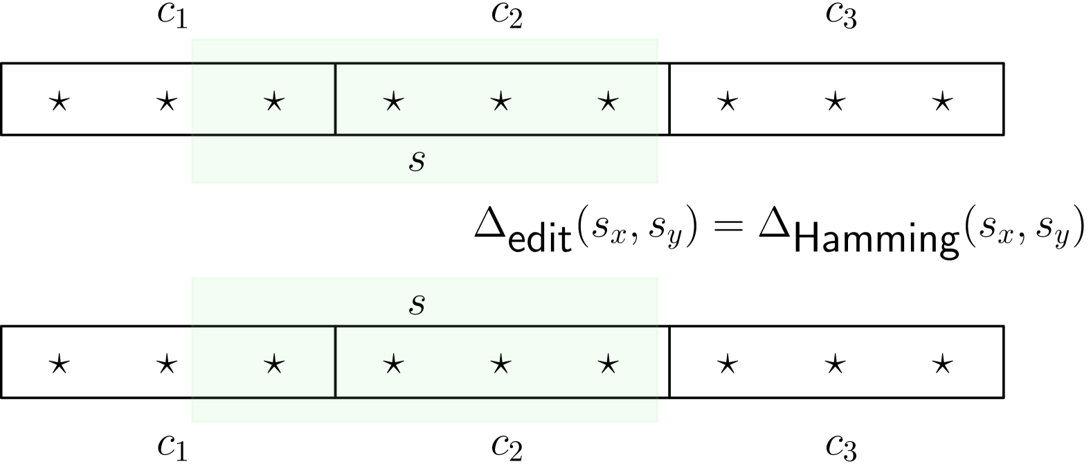
(a) For short intervals i.e., intervals of length at most $3m-2$, the misaligner guarantees isometry.

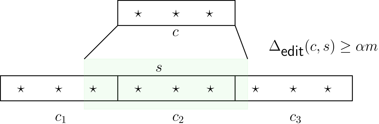
(b) The relative edit distance between a block and a substring coming from the concatenation of three blocks is at least $\alpha$.

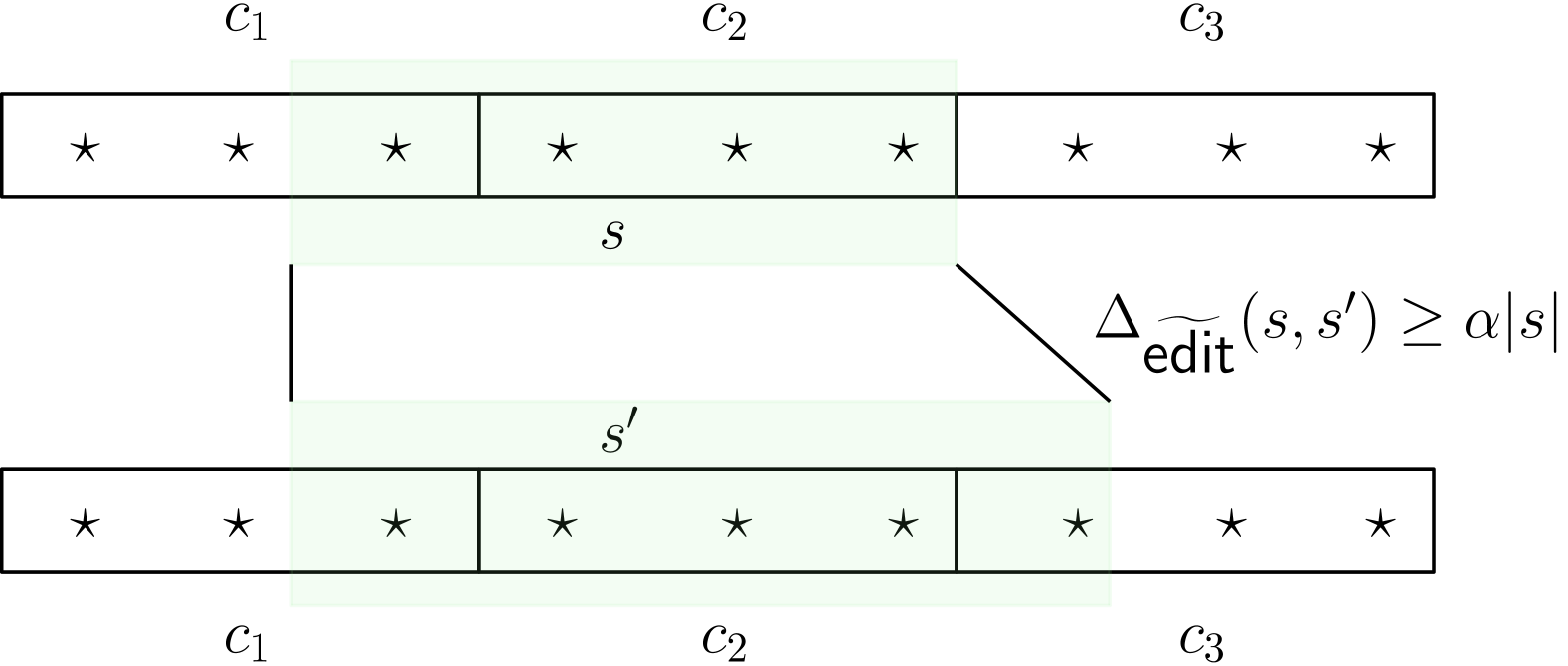
(c) The relative nowhere-vertical edit distance between the concatenation of a block suffix and a full block and its extension by some prefix of a block is at least $\alpha$.

Figure 6: Properties of the Misaligner

5 Locally Self-Matching Strings: Existence and Construction

In this section, we define locally self-matching strings, which are strings in which every substring has a small relative nowhere-vertical LCS.

Definition 5.1 ($\varepsilon$-locally self-matching strings).

For any $\varepsilon\in(0,1)$, a string $w$ is said to be $\varepsilon$-locally self-matching if for all substrings $s$ of $w$, we have $\widetilde{\textnormal{{LCS}}}(s,s)<\varepsilon|s|$.

We remark that locally self-matching strings are closely related to synchronization strings introduced by Haeupler and Shahrasbi [HS21b]. In fact, it is known that if $w$ is an $\varepsilon$-locally self-matching string, then it is also an $\varepsilon^{\prime}$-synchronization string where $\varepsilon^{\prime}=2\varepsilon$. The converse is also true: an $\varepsilon$-synchronization string is also an $\varepsilon$-locally self-matching string. Therefore, the notions are equivalent up to constant factors in the parameter $\varepsilon$. For our purposes, it is more convenient to use the formulation in Definition 5.1 than the more well-known synchronization string formulation.

It is known that for any $\varepsilon\in(0,1)$, arbitrarily long $\varepsilon$-locally self-matching strings exist over alphabets of size $\Theta\left(\frac{1}{\varepsilon^{2}}\right)$ [CHL⁺19]. However, to derive explicit bounds on the rate of our embedding, one needs to uncover the constants hiding inside the asymptotic notation. We do so in the following theorem by giving a much tighter analysis of Theorem 3.2 in [CHL⁺19].

Theorem 5.2.

Let $\Sigma$ be a finite set and $\varepsilon\in\left(0,\frac{1}{2}\right]$ such that the following holds:

$$|\Sigma|\geq\frac{e^{2}}{\varepsilon^{2}}\cdot\left(1+4\sqrt[4]{\varepsilon}\right).$$

Then, for all positive integers $n$, there exists a $\varepsilon$-locally self-matching string $w$ over $\Sigma$ of length $n$. Moreover, $w$ can be computed in $\textnormal{{poly}}(n)$ time.

Proof.

We prove this via the probabilistic method. Let $w$ be a string of length $n$ generated via the following random process.

Let $\theta:=\frac{e^{2}}{\varepsilon^{7/4}}$. Randomly pick $\lceil\theta\rceil$ different symbols from $\Sigma$ and let them be the first $\lceil\theta\rceil$ symbols of $w$. If $\lceil\theta\rceil\geq n$, we just pick $n$ different symbols. For $\lceil\theta\rceil+1\leq i\leq n$, we pick the $i^{\text{th}}$ symbol $w[i]$ uniformly randomly from $\Sigma\setminus\{w[i-1],\ldots,w[i-\lceil\theta\rceil+1]\}$.

We call a substring $s$ of $w$ bad if $\widetilde{\textnormal{{LCS}}}(s)\geq\varepsilon\cdot|s|$. Note that $s$ can be bad only if $|s|\geq\lceil\theta\rceil$. Let $\ell:=|s|$. We have,

$$\Pr[s\textnormal{ is bad}] \leq\binom{\ell}{\varepsilon\ell}^{2}(|\Sigma|-\lceil\theta\rceil)^{-\varepsilon\ell}$$

$$\leq{\left(\frac{e\ell}{\varepsilon\ell}\right)^{2\varepsilon\ell}(|\Sigma|-\theta)^{-\varepsilon\ell}}$$

$$=C^{-\varepsilon^{\prime}\ell},$$

where $\varepsilon^{\prime}:=2\varepsilon$ and $C=\frac{\varepsilon\cdot\sqrt{|\Sigma|-\theta}}{e}\geq\sqrt{1+3\sqrt[4]{\varepsilon}},$ where the inequality follows from the assumption on $|\Sigma|$ in the theorem statement. However, we have that for any $z\in(0,1)$:

$$(1+z)^{2}=1+2z+z^{2}\leq 1+2z^{3/4}+z^{3/2}\leq 1+3z^{3/4}.$$

We apply the above with $z=\varepsilon^{1/3}$ and by noting that $\varepsilon\in(0,0.5]$,

$$C\geq 1+\sqrt[3]{\varepsilon}.$$

We call $w$ good if none of its substrings are bad.

Lemma 5.3 ([CHL⁺19]).

The badness of two substrings $s$ and $s^{\prime}$ are mutually independent if $s$ and $s^{\prime}$ do not intersect.

By the Lovasz Local Lemma, the probability of $w$ being good is non-zero if for each substring $s$ of $w$, there exists $x_{s}\in(0,1)$ such that the following holds:

$$\Pr[s\textnormal{ is bad}]\leq x_{s}\cdot\prod_{s^{\prime}\textnormal{ intersects }s}(1-x_{s^{\prime}}).$$

We claim that $x_{s}:=D^{-\varepsilon^{\prime}|s|}$ works for some choice of $D$ to be determined later. Since the number of length $\ell$ substrings intersecting the substring $s$ is $\ell+|s|$, this amounts to showing that the following inequality is true for every substring $s$ of $w$.

$$C^{-\varepsilon^{\prime}|s|}\leq D^{-\varepsilon^{\prime}|s|}\cdot\prod_{\ell=\theta}^{n}(1-D^{-\varepsilon^{\prime}\ell})^{|s|+\ell}.$$

This inequality is equivalent to the following inequality for all substrings $s$.

$$C\geq\frac{D}{\prod_{\ell=\theta}^{n}(1-D^{-\varepsilon^{\prime}\ell})^{\frac{1+\ell/|s|}{\varepsilon^{\prime}}}}.$$

The right hand side of the inequality is maximized when $|s|=\lceil\theta\rceil$. So, it suffices to show that:

$$C\geq\frac{D}{\prod_{\ell=\theta}^{n}(1-D^{-\varepsilon^{\prime}\ell})^{\frac{\ell+\theta}{\theta\varepsilon^{\prime}}}}.$$ (1)

We set $D=1+0.9\cdot\sqrt[3]{\varepsilon}$. To show that (1) holds, we first prove the following:

$$\prod_{\ell=\theta}^{n}(1-D^{-\varepsilon^{\prime}\ell})^{\frac{\ell+\theta}{\theta\varepsilon^{\prime}}}\geq 1-\frac{\varepsilon^{7/4}}{e^{2}}.$$ (2)

We will show below that the following is true:

$$(1-D^{-\varepsilon^{\prime}\ell})^{\frac{\ell+\theta}{\theta\varepsilon^{\prime}}}\geq 1-\frac{1}{\ell^{2}}.$$ (3)

Let us first see that the above is sufficient to finish the proof. We first note the following identity (which can be verified by expanding the product):

$$\prod_{i=2}^{n}\left(1-\frac{1}{i^{2}}\right)=\frac{n+1}{2n}.$$

Therefore, we have that (2) holds:

$$\prod_{\ell=\theta}^{n}(1-D^{-\varepsilon^{\prime}\ell})^{\frac{\ell+\theta}{\theta\varepsilon^{\prime}}}\geq\prod_{\ell=\theta}^{n}\left(1-\frac{1}{\ell^{2}}\right)=\frac{\frac{n+1}{2n}}{\frac{\theta}{2\theta-2}}\geq 1-\frac{1}{\theta}\geq 1-\frac{\varepsilon^{7/4}}{e^{2}}.$$

We can now verify that (1) holds:

$$\frac{1}{C}\cdot\frac{D}{\prod_{\ell=\theta}^{n}(1-D^{-\varepsilon^{\prime}\ell})^{\frac{\ell+\theta}{\theta\varepsilon^{\prime}}}} \leq\frac{1+0.9\cdot\sqrt[3]{\varepsilon}}{1-\frac{\varepsilon^{7/4}}{e^{2}}}\cdot\frac{1}{1+\sqrt[3]{\varepsilon}}=\frac{1+0.9\cdot\sqrt[3]{\varepsilon}}{1+\sqrt[3]{\varepsilon}-\frac{\varepsilon^{7/4}}{e^{2}}-\frac{\varepsilon^{25/12}}{e^{2}}}$$

$$\leq\frac{1+0.9\cdot\sqrt[3]{\varepsilon}}{1+\sqrt[3]{\varepsilon}\cdot\left(1-\frac{1}{2^{17/12}\cdot e^{2}}-\frac{1}{2^{7/4}\cdot e^{2}}\right)}<\frac{1+0.9\cdot\sqrt[3]{\varepsilon}}{1+0.909\cdot\sqrt[3]{\varepsilon}}<1,$$

where we have used that $\varepsilon\leq 0.5$.

Thus, we are left to show (3), we have:

$$\left(1-D^{-\varepsilon^{\prime}\ell}\right)^{\frac{\ell+\theta}{\theta\varepsilon^{\prime}}}\geq 1-\frac{\ell+\theta}{\varepsilon^{\prime}\theta}\cdot D^{-\varepsilon^{\prime}\ell}.$$

First notice that the function $f(\ell):=\frac{(\ell+\theta)\ell^{2}}{\varepsilon^{\prime}\theta}\cdot D^{-\varepsilon^{\prime}\ell}$ is decreasing for all $\ell\geq\theta$. To see this note that:

$$f(\ell+1)=\frac{(\ell+1+\theta)(\ell+1)^{2}}{\varepsilon^{\prime}\theta}\cdot D^{-\varepsilon^{\prime}(\ell+1)}=D^{-\varepsilon^{\prime}}\cdot\frac{(\ell+1+\theta)(\ell+1)^{2}}{(\ell+\theta)\ell^{2}}\cdot f(\ell).$$

With the goal of relating $f(\ell)$ and $f(\ell+1)$, we compute:

$$D^{-\varepsilon^{\prime}}\cdot\left(1+\frac{1}{\ell+\theta}\right)\cdot\left(1+\frac{1}{\ell}\right)^{2}<D^{-\varepsilon^{\prime}}\cdot\left(1+\frac{1}{\theta}\right)^{3}\leq D^{-\varepsilon^{\prime}}\cdot\left(1+\frac{4}{\theta}\right),$$

where the last inequality follows because $\theta\geq 4$. Thus, we have shown that $f(\ell+1)=f(\ell)\cdot D^{-\varepsilon^{\prime}}\cdot\left(1+\frac{4}{\theta}\right)$. We will now argue that $D^{-\varepsilon^{\prime}}\cdot\left(1+\frac{4}{\theta}\right)<1$.

Claim 5.4.

We have $\left(1+0.9\sqrt[3]{\varepsilon}\right)^{2\varepsilon}>1+\frac{4\varepsilon^{7/4}}{e^{2}}$ for $\varepsilon\in(0,0.5]$.

Proof.

We have from the Taylor series expansion for $\ln(1+x)$ that for $x\in(0,1)$:

$$\ln(1+x)\geq x-\frac{x^{2}}{2}.$$ (4)

Then, we have:

$$2\varepsilon\cdot\ln\left(1+0.9\sqrt[3]{\varepsilon}\right)\geq 2\varepsilon\cdot\left(0.9\sqrt[3]{\varepsilon}-\frac{\left(0.9\sqrt[3]{\varepsilon}\right)^{2}}{2}\right)=1.8\cdot\varepsilon^{4/3}-0.81\cdot\varepsilon^{5/3}.$$

Exponentiating both sides gives us:

$$\left(1+0.9\sqrt[3]{\varepsilon}\right)^{2\varepsilon}\geq e^{1.8\cdot\varepsilon^{4/3}-0.81\cdot\varepsilon^{5/3}}.$$ (5)

Again from the Taylor Expansion of $e^{u}$ for any $u\in(0,1)$ we have:

$$e^{u}\geq 1+u+\frac{u^{2}}{2}.$$

Therefore,

$$e^{1.8\cdot\varepsilon^{4/3}-0.81\cdot\varepsilon^{5/3}}\geq 1+1.8\cdot\varepsilon^{4/3}-0.81\cdot\varepsilon^{5/3}+1.62\cdot\varepsilon^{8/3}-1.458\cdot\varepsilon^{3}+0.32805\cdot\varepsilon^{10/3}.$$ (6)

Let $f(\varepsilon):=1.25\cdot\varepsilon^{4/3}-0.81\cdot\varepsilon^{5/3}+1.62\cdot\varepsilon^{8/3}-1.458\cdot\varepsilon^{3}+0.32805\cdot\varepsilon^{10/3}$. The derivative $f^{\prime}(\varepsilon)$ is:

$$f^{\prime}(\varepsilon)=\frac{5}{3}\varepsilon^{1/3}-1.35\varepsilon^{2/3}+{4.32}\varepsilon^{5/3}-4.374\varepsilon^{2}+1.0935\varepsilon^{7/3}$$

Since $1.35\varepsilon^{2/3}<1.35\varepsilon^{1/3}$ and $4.374\varepsilon^{2}<{4.32}\varepsilon^{5/3}+0.06\varepsilon^{1/3}$ when $\varepsilon\in(0,0.5]$, we have:

$$f^{\prime}(\varepsilon)>\left(\frac{5}{3}-1.41\right)\cdot\varepsilon^{1/3}+1.0935\cdot\varepsilon^{7/3}>0,$$

and thus we have $f$ is strictly increasing in $(0,0.5]$, and $f(0)=0$, we have that $f(\varepsilon)>0$ for all $\varepsilon\in(0,0.5]$. Returning to (6), we have:

$$e^{1.8\cdot\varepsilon^{4/3}-0.81\cdot\varepsilon^{5/3}}\geq 1+0.55\cdot\varepsilon^{4/3}+f(\varepsilon)>1+0.55\cdot\varepsilon^{4/3}>1+0.55\cdot\varepsilon^{7/4}>1+\frac{4}{e^{2}}\cdot\varepsilon^{7/4}.$$

The proof then follows from (5). ∎

Thus, we have proved that $f(\ell+1)<f(\ell)$. Returning to proving (2) we have:

$$(1-D^{-\varepsilon^{\prime}\ell})^{\frac{\ell+\theta}{\theta\varepsilon^{\prime}}}\geq 1-\frac{f(\ell)}{\ell^{2}}\geq 1-\frac{f(\theta)}{\ell^{2}}.$$

The proof concludes now because we claim that $f(\theta)<1$

Claim 5.5.

We have $f(\theta)=\frac{2\theta^{2}}{\varepsilon^{\prime}}\cdot D^{-\varepsilon^{\prime}\theta}<1$ for all $\varepsilon\in(0,0.5]$.

Proof.

We can rewrite (4) as follows:

$$(1+x)^{1/x}\geq e^{1-\frac{x}{2}}.$$

Thus, we have that:

$$D^{\varepsilon^{\prime}\theta}=D^{\frac{2e^{2}}{\varepsilon^{3/4}}}=\left(\left(1+0.9\sqrt[3]{\varepsilon}\right)^{\frac{10}{9\sqrt[3]{\varepsilon}}}\right)^{\frac{1.8e^{2}}{\varepsilon^{5/12}}}\geq e^{\left(1-0.45\sqrt[3]{\varepsilon}\right)\cdot{\frac{1.8e^{2}}{\varepsilon^{5/12}}}}=e^{\frac{1.8e^{2}}{\varepsilon^{5/12}}-{\frac{0.81\cdot e^{2}}{\varepsilon^{1/12}}}}>e^{\frac{1.8e^{2}}{\varepsilon^{5/12}}-{\frac{0.81\cdot e^{2}}{\varepsilon^{5/12}}}}=e^{\frac{0.99e^{2}}{\varepsilon^{5/12}}}.$$

On the other hand, we have that

$$\frac{2\theta^{2}}{\varepsilon^{\prime}}=\frac{\theta^{2}}{\varepsilon}=\frac{e^{4}}{\varepsilon^{4.5}}<\frac{54.6}{\varepsilon^{4.5}}.$$

Thus proving the claim simply amounts to showing the below holds for all $\varepsilon\in(0,0.5]$:

$$\left(e^{\frac{0.99e^{2}}{\varepsilon^{5/12}}}\right)^{2}\geq\left(\frac{54.6}{\varepsilon^{4.5}}\right)^{2}\iff e^{\frac{1.98e^{2}}{\varepsilon^{5/12}}}\geq\frac{2982}{\varepsilon^{9}}.$$

The Maclaurin series tells us that:

$$e^{x}=\sum_{k=0}^{\infty}{\frac{x^{k}}{k!}}=1+x+{\frac{x^{2}}{2!}}+{\frac{x^{3}}{3!}}+\cdots$$

By looking at the Maclaurin series and only picking the twenty-third term we have:

$$e^{\frac{1.98e^{2}}{\varepsilon^{5/12}}}>\left(\frac{1.98e^{2}}{\varepsilon^{5/12}}\right)^{22}\cdot\frac{1}{22!}>\frac{38443}{\varepsilon^{55/6}}>\frac{38443}{\varepsilon^{9}}>\frac{2982}{\varepsilon^{9}}.$$

The $\textnormal{poly}(n)$-time construction can be done by considering algorithmic versions of the Lovasz Local Lemma. For details, the reader is referred to Lemma 3.3 in [CHL⁺19]. ∎

Remark 5.6.

Note that in the proof, we set $\theta\geq\frac{e^{2}}{\varepsilon^{7/4}}>3$. Therefore, every three consecutive symbols in the string whose existence we prove are distinct.

6 Embeddings via Misaligners

In this section, we show how to get an embedding using misaligners and locally self-matching strings. On a high level, this embedding takes a locally self-matching string and replaces each of its symbols with elements of some misaligner. This results in a binary string with wildcards. To embed some input string $x$, we then simply instantiate this wildcard string with $x$. Details follow.

Let $\mathcal{C}$ be a $(m,k,t,\alpha)$-misaligner and $\Sigma$ be an alphabet such that $|\Sigma|=k$. Fix some arbitrary bijection $\sigma$ from $\Sigma$ to $\mathcal{C}$. Given $\mathcal{C}$ and a positive integer $n$, we compute our embedding map as follows. First, we find the smallest integer $N$ such that $N\geq\frac{tn}{m}$. Next by Theorem 5.2, we compute an $\varepsilon$-locally self-matching string $w$ over $\Sigma$ of length $N$, where $k\geq\frac{e^{2}}{\varepsilon^{2}}\cdot\left(1+4\sqrt[4]{\varepsilon}\right)$. Then for every symbol $c$ in $w$, we replace it by $\sigma(c)\in\mathcal{C}$ to obtain the string $w^{\prime}$. Note that $w^{\prime}$ has length $mN\geq tn$, and since every string in $\mathcal{C}$ has one wildcard symbol in every $t$ symbols, $w^{\prime}$ has at least $n$ wildcard symbols. Next, we delete sufficiently many symbols from the right end of $w^{\prime}$ to ensure that $w^{\prime}$ has length exactly $tn$ and contains exactly $n$ wildcard symbols. Finally, for every $x\in\{0,1\}^{n}$, we define $\varphi_{\mathcal{C},w,n}(x):=w^{\prime}_{x}$, i.e., we define $\varphi_{\mathcal{C},w,n}(x)$ to be the string obtained by instantiating $w^{\prime}$ by $x$. Clearly, $\varphi_{\mathcal{C},w,n}:\{0,1\}^{n}\to\{0,1\}^{tn}$ has rate $\frac{1}{t}$. We now make the following claim.

Theorem 6.1.

Let $\mathcal{C}$ be a $(m,k,t,\alpha)$-misaligner and $w$ be an $\varepsilon$-locally self-matching string such that $t\geq\frac{1}{(1-\varepsilon)\alpha-\frac{1}{3m-1}}$. Then for every positive integer $n$ and $x,y\in\{0,1\}^{n}$, we have $\Delta_{\textnormal{{edit}}}\left(\varphi_{\mathcal{C},w,n}(x),\varphi_{\mathcal{C},w,n}(y)\right)=\Delta_{\textnormal{{Hamming}}}(x,y)$.

7 Proof of Theorem 6.1

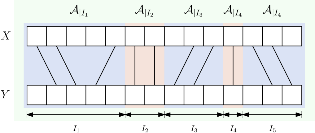
Figure 7: An edit distance alignment $\mathcal{A}$ between the strings $X$ and $Y$. Note the alternating maximal nowhere-vertical and vertical intervals (highlighted blue and red, respectively) $I_{1},I_{2},I_{3},I_{4}$ and $I_{5}$ under $\mathcal{A}$. For each $I\in\{I_{1},I_{2},I_{3},I_{4},I_{5}\}$, the induced alignment $\mathcal{A}_{|I}$ is an edit distance alignment between $X_{|I}$ and $Y_{|I}$.

Proof of Theorem 6.1.

Assume for the sake of contradiction that there exist a positive integer $n$ and strings $x,y\in\{0,1\}^{n}$ such that $\Delta_{\textnormal{{edit}}}(\varphi_{\mathcal{C},w,n}(x),\varphi_{\mathcal{C},w,n}(y))<\Delta_{\textnormal{{Hamming}}}(x,y)$. Let $X=\varphi_{\mathcal{C},w,n}(x)$, $Y=\varphi_{\mathcal{C},w,n}(y)$ and consider any optimal edit distance alignment $\mathcal{A}$ between $X$ and $Y$. By assumption, we have $\textnormal{{cost}}(\mathcal{A})<\Delta_{\textnormal{{Hamming}}}(X,Y)$. Call a non-empty interval $I\subseteq[1,tn]$ vertical under $\mathcal{A}$ if for every $i\in I$, $\mathcal{A}$ aligns $X[i]$ to $Y[i]$. Similarly, call $I$ nowhere-vertical under $\mathcal{A}$ if for no $i\in I$, $\mathcal{A}$ aligns $X[i]$ to $Y[i]$. Note that an interval could be neither vertical nor nowhere-vertical. The key observation is that $\mathcal{A}$ naturally induces a partition of $[1,tn]$ into alternating maximal vertical and maximal nowhere-vertical intervals, i.e., there exists a unique sequence of intervals $I_{1}<I_{2}<\ldots<I_{j}$ for some integer $j$ such that $I_{1}\cup I_{2}\cup\cdots\cup I_{j}=[1,tn]$, every interval in the sequence is either vertical or nowhere-vertical, and two consecutive intervals are of different types. Additionally, for every $I\in\{I_{1},I_{2},\ldots,I_{j}\}$, the alignment $\mathcal{A}$ induces an edit distance alignment between $X_{|I}$ and $Y_{|I}$ (See Figure 7). For every $I\in\{I_{1},I_{2},\ldots,I_{j}\}$, we refer to the alignment between $X_{I}$ and $Y_{I}$ induced by $\mathcal{A}$ as $\mathcal{A}_{|I}$ and its cost as $\textnormal{{cost}}(\mathcal{A}_{|I})$. Note that $\textnormal{{cost}}(\mathcal{A})=\sum_{I\in\{I_{1},I_{2},\ldots,I_{j}\}}\textnormal{{cost}}(\mathcal{A}_{|I})$. By assumption, we have,

$$\sum_{I\in\{I_{1},I_{2},\ldots,I_{j}\}}\textnormal{{cost}}(\mathcal{A}_{|I})=\textnormal{{cost}}(\mathcal{A})<\Delta_{\textnormal{{Hamming}}}(X,Y)=\sum_{I\in\{I_{1},I_{2},\ldots,I_{j}\}}\Delta_{\textnormal{{Hamming}}}(X_{|I},Y_{|I})$$

Therefore, there must exist $I\in\{I_{1},I_{2},\ldots,I_{j}\}$ such that $\textnormal{{cost}}(\mathcal{A}_{|I})<\Delta_{\textnormal{{Hamming}}}(X_{|I},Y_{|I})$. We show that this is impossible if the parameters of the misaligner $\mathcal{C}$ and the locally self-matching string $w$ are chosen in a way such that $t\geq\frac{1}{(1-\varepsilon)\alpha-\frac{1}{3m-1}}$ holds.

First note that $I$ must be a nowhere-vertical interval under $\mathcal{A}$ since otherwise, we have $\textnormal{{cost}}(\mathcal{A}_{|I})=\Delta_{\textnormal{{Hamming}}}(X_{|I},Y_{|I})$. Further note that $|I|>3m-2$ since otherwise, by Property 2 of misaligners, $\textnormal{{cost}}(\mathcal{A}_{|I})=\Delta_{\widetilde{\textnormal{{edit}}}}(X_{|I},Y_{|I})\geq\Delta_{\textnormal{{edit}}}(X_{|I},Y_{|I})=\Delta_{\textnormal{{Hamming}}}(X_{|I},Y_{|I})$. To derive the desired contradiction, we start by lower bounding $\textnormal{{cost}}(\mathcal{A}_{|I})$. The first step of the lower-bounding process involves reinstantiating the wildcard symbols in $X_{|I}$ and $Y_{|I}$ to minimize their nowhere-vertical edit distance. More precisely, let $J\subseteq[|I|]$ be the set of indices in $X_{|I}$ and $Y_{|I}$ that originally contained the symbol $\star$ and were later replaced by symbols of $x$ and $y$ during the embedding. Define $S$ to be the string (with wildcards) obtained by taking $X_{|I}$ (or equivalently $Y_{|I}$) and replacing, for each $j\in J$, $X_{|_{I}}[j]$ with the symbol $\star$. Then let $x^{*},y^{*}\in\{0,1\}^{\Gamma(S)}$ be strings minimizing $\Delta_{\widetilde{\textnormal{{edit}}}}(S_{x^{*}},S_{y^{*}})$. Finally, set $X^{*}:=S_{x^{*}}$, $Y^{*}:=S_{y^{*}}$ and let $\mathcal{A}^{*}$ be an optimal nowhere-vertical edit distance alignment between $X^{*}$ and $Y^{*}$. See Figure 8 for a description of this entire process.

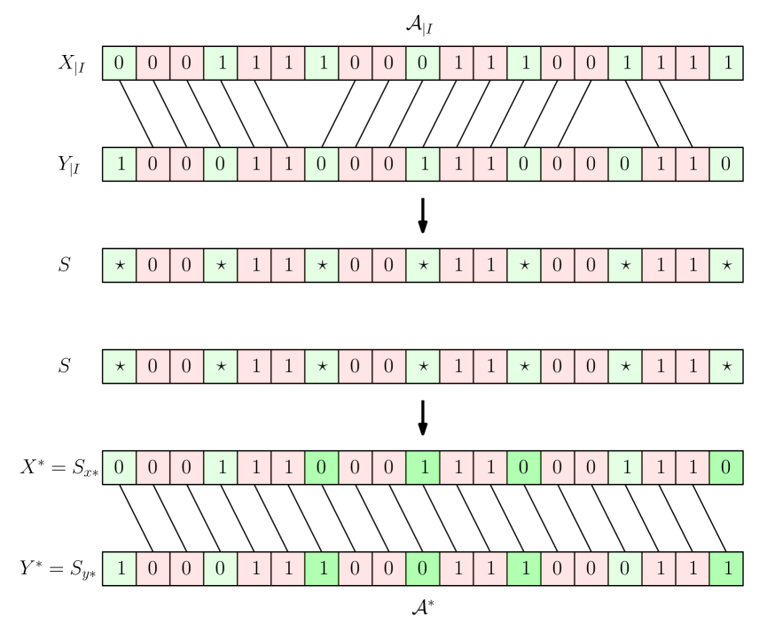
Figure 8: The reinstantiation process. We start with the strings $X_{|I}$ and $Y_{|I}$, replace back the $\star$ symbols where they originally were (marked green) to obtain the string $S$, and reinstantiate $S$ with the strings $x^{*}$ and $y^{*}$ to ensure that $\Delta_{\widetilde{\textnormal{{edit}}}}(S_{x^{*}},S_{y^{*}})$ is minimized. Symbols that have changed in the reinstantiation process have been highlighted with a darker shade of green.

Clearly, $\textnormal{{cost}}_{X_{|I}}^{Y_{|I}}(\mathcal{A}_{|I})\geq\textnormal{{cost}}_{X^{*}}^{Y^{*}}(\mathcal{A}^{*})$. So, by assumption, $\textnormal{{cost}}_{X^{*}}^{Y^{*}}(\mathcal{A}^{*})<\Delta_{\textnormal{{Hamming}}}(X_{|I},Y_{|I})$ holds. Call a string a block if it is the instantiation of some element in $\mathcal{C}$. Note that both $X^{*}$ and $Y^{*}$ start with some proper suffix (possibly empty) of a block, followed by a sequence of blocks and end in a proper prefix (again possibly empty). Let $p$ be the number of blocks in $X^{*}$ (not counting the starting and ending partial blocks). Let $b_{1},b_{2},\ldots,b_{p}$ the blocks of $X^{*}$ in order. Note that since $|I|>3m-2$, $p\geq 2$ and $b_{1}$ and $b_{p}$ are distinct. Additionally, let $b_{0}$ and $b_{p+1}$ be the starting and ending partial blocks, respectively, of $X^{*}$. Similarly name the blocks of $Y^{*}$ as $b^{\prime}_{0},b^{\prime}_{1},b^{\prime}_{2},\ldots,b^{\prime}_{p},b^{\prime}_{p+1}$. The alignment $\mathcal{A}^{*}$ specifies a sequence of edit operations on $X^{*}$ transforming it into $Y^{*}$. This sequence naturally induces on each $b_{i}$, where $0\leq i\leq p+1$, a sequence of edit operations that transforms it into some string $s_{i}$, where we have $s_{0}\circ s_{1}\circ\ldots\circ s_{p}\circ s_{p+1}=Y^{*}$. Note that we have —

$$\textnormal{{cost}}(\mathcal{A}^{*})\geq\sum_{i=0}^{p+1}\Delta_{\textnormal{{edit}}}(b_{i},s_{i})$$

We now start to lower bound $\textnormal{{cost}}(\mathcal{A}^{*})$. We begin with the following observation.

Observation 7.1.

There exists a string $Y^{\prime}$ obtained by re-instantiating some blocks of $Y^{*}$, and an alignment $\mathcal{A}^{\prime}$ transforming $X^{*}$ to $Y^{\prime}$, such that the following holds:

1. Let $b_{i},b^{\prime}_{i^{\prime}}$ be instantiations of the same codeword in $\mathcal{C}$, where $i\neq i^{\prime}$ , then in the alignment $\mathcal{A}^{\prime}$, if any one pair of characters between $b_{i}$ and $b^{\prime}_{i^{\prime}}$ is matched badly, all the pairs are matched badly.

2. The cost of the new alignment does not increase:

   $$\textnormal{{cost}}_{X^{*}}^{Y^{\prime}}(\mathcal{A}^{\prime})\leq\textnormal{{cost}}_{X^{*}}^{Y^{*}}(\mathcal{A}^{*}).$$

Proof.

We construct sequences $Y^{0},Y^{1},\dots,Y^{p}$ and $\mathcal{A}^{0},\mathcal{A}^{1},\dots,\mathcal{A}^{p}$, starting with $Y^{0}=Y^{*}$ and $\mathcal{A}^{0}=\mathcal{A}^{*}$, and ending with $Y^{p}=Y^{\prime}$ and $\mathcal{A}^{p}=\mathcal{A}^{\prime}$. For each block $b_{i}$ in $X^{*}$ (from $i=1$ to $p$), we update $Y^{i}$ and $\mathcal{A}^{i}$ as follows:

1. If $b_{i}$ has no badly matched pairs in $\mathcal{A}^{i-1}$, set $Y^{i}=Y^{i-1}$ and $\mathcal{A}^{i}=\mathcal{A}^{i-1}$.

2. If $b_{i}$ has a badly matched pair with $b^{\prime}_{i^{\prime}}$ (for $i\neq i^{\prime}$ and both instantiations of the same $c\in\mathcal{C}$):

   1. Re-instantiate $b^{\prime}_{i^{\prime}}$: Set $b^{\prime}_{i^{\prime}}:=b_{i}$ in $Y^{i}$.

   2. Modify the Alignment: Update $\mathcal{A}^{i-1}$ to obtain $\mathcal{A}^{i}$ by:

      • Aligning the entire $b_{i}$ to $b^{\prime}_{i^{\prime}}$, matching $b_{i}[k]$ to $b^{\prime}_{i^{\prime}}[k]$ for all $k\in[m]$.

      • Removing any other pair that are in $\mathcal{A}^{i-1}$ and involves $b_{i}$ or $b^{\prime}_{i^{\prime}}$ that are not part of this full block alignment.

      • Keeping all other pairs unchanged.

It is easy to see that, after each round $\mathcal{A}^{i}$ is a still a valid alignment.

Cost Analysis:

We need to show that the cost does not increase after each round:

$$\textnormal{{cost}}_{X^{*}}^{Y^{i}}(\mathcal{A}^{i})\leq\textnormal{{cost}}_{X^{*}}^{Y^{i-1}}(\mathcal{A}^{i-1}).$$

This follows from the following claim.

Claim 7.2.

Let $P$ and $Q$ be strings, and suppose we have an alignment $\chi$ between $P$ and $Q$, where $P[i]$ is matched to $Q[j]$, but $P[i-1]$ is not matched to $Q[j-1]$. Let $Q^{\prime}$ be the string obtained by modifying $Q[j-1]$ to be equal to $P[i-1]$ if they are not equal; otherwise, $Q^{\prime}=Q$. Then, we can modify $\chi$ to obtain a new alignment $\chi^{\prime}$ between $P$ and $Q^{\prime}$, where $P[i-1]$ is matched to $Q^{\prime}[j-1]$, and the cost does not increase:

$$\textnormal{{cost}}_{P}^{Q^{\prime}}(\chi^{\prime})\leq\textnormal{{cost}}_{P}^{Q}(\chi).$$

The claim can be easily proved using some simple case analysis, left as an exercise for the reader.

Applying this claim iteratively for each position $k$ from $j$ down to $1$ (and similarly from $j$ up to $m$), we can extend the alignment between $b_{i}$ and $b^{\prime}_{i^{\prime}}$ to the entire block without increasing the cost.

Therefore, after processing all blocks with bad edges, the total cost satisfies:

$$\textnormal{{cost}}_{X^{*}}^{Y^{\prime}}(\mathcal{A}^{\prime})\leq\textnormal{{cost}}_{X^{*}}^{Y^{*}}(\mathcal{A}^{*}).\qed$$

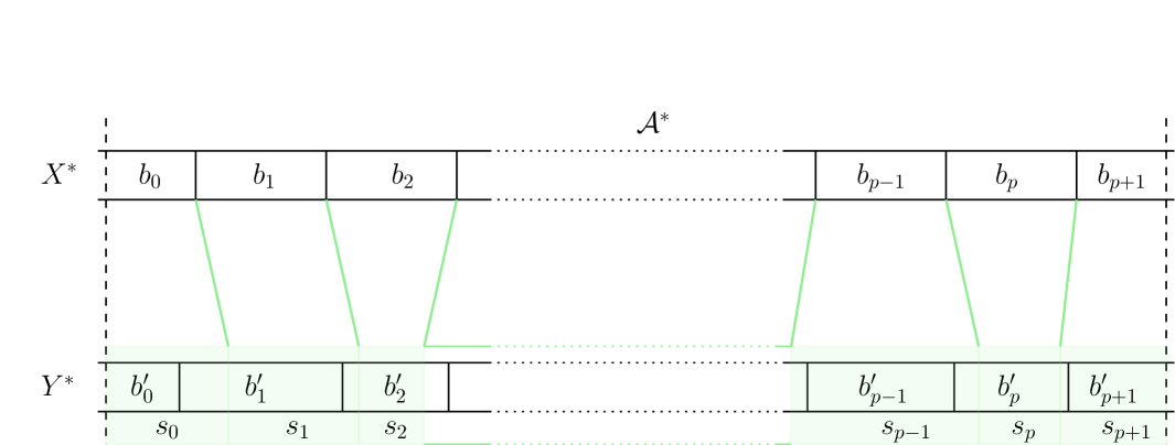
Figure 9: An optimal nowhere-vertical alignment $\mathcal{A}^{*}$ between $X^{*}$ and $Y^{*}$ specifies a sequence of edit operations that transforms each block $b_{i}$, where $0\leq i\leq p+1$, into a string $s_{i}$ such that $s_{0}\circ s_{1}\circ\ldots\circ s_{p}\circ s_{p+1}=Y^{*}$.

For the remainder of the proof, we assume without loss of generality that $Y^{*}=Y^{\prime}$, $\mathcal{A}^{*}=\mathcal{A}^{\prime}$ where $Y^{\prime}$ and $\mathcal{A}^{\prime}$ are the string and the alignment guaranteed to exist by Observation 7.1. For each $i\in[p]$, call a block $b_{i}$ of $X^{*}$ bad, if $\mathcal{A}^{*}$ aligns $b_{i}$ to some block $b^{\prime}_{i^{\prime}}$ completely and $b_{i}=b^{\prime}_{i^{\prime}}$. From the set of bad blocks $b_{i}$ and their matches $b^{\prime}_{i^{\prime}}$, one can recover a nowhere-vertical common subsequence of a length $p$ substring of $w$. Since $w$ is a $\varepsilon$-locally self-matching string, it follows that the number of bad blocks in $X^{*}$ is at most $\varepsilon p$.

Next, call a block $b_{i}$ of $X^{*}$ overworked if $|s_{i}|\geq(1+\alpha)m$. Call the rest of the blocks in $X^{*}$ good. We have the following observations.

Observation 7.3.

If $b_{i}$ is a bad block, then $\Delta_{\textnormal{{edit}}}(b_{i},s_{i})=0$.

Proof.

This follows from the definition of a bad block. ∎

Observation 7.4.

If a block $b_{i}$ is either overworked or good, then $\Delta_{\textnormal{{edit}}}(b_{i},s_{i})\geq\alpha m$

Proof.

If $b_{i}$ is overworked, then $\Delta_{\textnormal{{edit}}}(b_{i},s_{i})\geq|s_{i}|-|b_{i}|\geq\alpha m$. If $b_{i}$ is good, then since $|s_{i}|<(1+\alpha)m<2m$, $s_{i}$ can intersect at most three consecutive blocks in $Y^{*}$. Let us call these blocks $b^{\prime}_{i^{\prime}-1},b^{\prime}_{i^{\prime}}$ and $b^{\prime}_{i^{\prime}+1}$ for some $i^{\prime}\in[p]$. By Remark 5.6, all three of these blocks are instantiations of distinct elements from $\mathcal{C}$. Now let $c_{i},c_{i^{\prime}-1},c_{i^{\prime}},c_{i^{\prime}+1}\in\mathcal{C}$ be strings such that $b_{i},b^{\prime}_{i^{\prime}-1},b^{\prime}_{i^{\prime}},b^{\prime}_{i^{\prime}+1}$ are instantiations of $c_{i},c_{i^{\prime}-1},c_{i^{\prime}},c_{i^{\prime}+1}$, respectively. If none of $c_{i^{\prime}-1},c_{i^{\prime}},c_{i^{\prime}+1}$ are equal to $c_{i}$, then by Property 3a of misaligners, we have $\Delta_{\textnormal{{edit}}}(b_{i},s_{i})\geq\alpha m$. Furthermore, if exactly one, say $c_{i^{\prime}-1}$ is equal to $c_{i}$, then there does not exist $j\in[m]$ such that $\mathcal{A}^{*}$ aligns $b_{i}[j]$ to $b^{\prime}_{i^{\prime}-1}[j]$ since otherwise, by Observation 7.1 and our assumption on $\mathcal{A}^{*}$, $b_{i}$ would be a bad block. Therefore, we can apply Property 3b to get $\Delta_{\textnormal{{edit}}}(b_{i},s_{i})\geq\alpha m$. ∎

We also have the following observations regarding the first partial block $b_{0}$.

Observation 7.5.

If $b_{1}$ is a bad block, then $\Delta_{\textnormal{{edit}}}(b_{0},s_{0})\geq\alpha|b_{0}|$

Proof.

If $b_{1}$ is a bad block, then $b^{\prime}_{0}\circ b^{\prime}_{1}$ is a prefix of $s_{0}$. Since $\alpha<1$, $|s_{0}|\geq|b^{\prime}_{0}\circ b^{\prime}_{1}|\geq(1+\alpha)|b_{0}|$. So, $\Delta_{\textnormal{{edit}}}(b_{0},s_{0})\geq|s_{0}|-|b_{0}|\geq\alpha b_{0}$. ∎

Observation 7.6.

If $b_{1}$ is not a bad block, then $\Delta_{\textnormal{{edit}}}(b_{0}\circ b_{1},s_{0}\circ s_{1})\geq\alpha(|b_{0}|+|b_{1}|)$.

Proof.

If $|s_{0}\circ s_{1}|\geq(1+\alpha)(|b_{0}|+|b_{1}|)$, then we are done. If $|s_{0}\circ s_{1}|<(1+\alpha)(|b_{0}|+|b_{1}|)$, then since $\alpha\leq\frac{1}{2}$, $s_{0}\circ s_{1}$ must be a prefix of $b^{\prime}_{0}\circ b^{\prime}_{1}\circ b^{\prime}_{2}$. By Property 4a of misaligners, it then follows that $\Delta_{\textnormal{{edit}}}(b_{0}\circ b_{1},s_{0}\circ s_{1})\geq\alpha(|b_{0}|+|b_{1}|)$. ∎

Similar statements for the final partial block $b_{p+1}$ also hold with essentially the same proofs.

Observation 7.7.

If $b_{p}$ is a bad block, then $\Delta_{\textnormal{{edit}}}(b_{p+1},s_{p+1})\geq\alpha|b_{p+1}|$

Observation 7.8.

If $b_{p}$ is not a bad block, then $\Delta_{\textnormal{{edit}}}(b_{p}\circ b_{p+1},s_{p}\circ s_{p+1})\geq\alpha(|b_{p}|+|b_{p+1}|)$.

We can now give a lower bound for $\textnormal{{cost}}(\mathcal{A}^{*})$. We claim the following.

Claim 7.9.

$\textnormal{{cost}}(\mathcal{A}^{*})\geq(1-\varepsilon)\alpha|I|$

Proof.

We break it the proof into four cases depending on whether or not $b_{1}$ and $b_{p}$ are bad.

• Case 1: Both $b_{1}$ and $b_{p}$ are bad.

  In this case, we have:

  $$\textnormal{{cost}}(\mathcal{A}^{*}) \geq\sum_{i=0}^{p+1}\Delta_{\textnormal{{edit}}}(b_{i},s_{i})$$

  $$=\Delta_{\textnormal{{edit}}}(b_{0},s_{0})+\Delta_{\textnormal{{edit}}}(b_{p+1},s_{p+1})+\sum_{i=1}^{p}\Delta_{\textnormal{{edit}}}(b_{i},s_{i})$$

  $$\geq\alpha|b_{0}|+\alpha|b_{p+1}|+\left(\sum_{\begin{subarray}{c}{b_{i}\textnormal{ is bad}}\\ {1\leq i\leq p}\end{subarray}}\Delta_{\textnormal{{edit}}}(b_{i},s_{i})+\sum_{\begin{subarray}{c}{b_{i}\textnormal{ is not bad}}\\ {1\leq i\leq p}\end{subarray}}\Delta_{\textnormal{{edit}}}(b_{i},s_{i})\right)$$

  $$\geq\alpha(|b_{0}|+|b_{p+1}|)+(0+(1-\varepsilon)p\alpha m)$$

  $$\geq(1-\varepsilon)\alpha(|b_{0}|+|b_{p+1}|)+(1-\varepsilon)p\alpha m$$

  $$=(1-\varepsilon)\alpha(|b_{0}|+|b_{p+1}|+pm)$$

  $$=(1-\varepsilon)\alpha|I|$$

• Case 2: $b_{p}$ is bad but $b_{1}$ is not.

  In this case, we have:

  $$\textnormal{{cost}}(\mathcal{A}^{*}) \geq\sum_{i=0}^{p+1}\Delta_{\textnormal{{edit}}}(b_{i},s_{i})$$

  $$=\Delta_{\textnormal{{edit}}}(b_{0}\circ b_{1},s_{0}\circ s_{1})+\Delta_{\textnormal{{edit}}}(b_{p+1},s_{p+1})+\sum_{i=2}^{p}\Delta_{\textnormal{{edit}}}(b_{i},s_{i})$$

  $$\geq\alpha(|b_{0}|+|b_{1}|)+\alpha|b_{p+1}|+\left(\sum_{\begin{subarray}{c}{b_{i}\textnormal{ is bad}}\\ {2\leq i\leq p}\end{subarray}}\Delta_{\textnormal{{edit}}}(b_{i},s_{i})+\sum_{\begin{subarray}{c}{b_{i}\textnormal{ is not bad}}\\ {2\leq i\leq p}\end{subarray}}\Delta_{\textnormal{{edit}}}(b_{i},s_{i})\right)$$

  $$\geq\alpha(|b_{0}|+b_{p+1})+\alpha|b_{1}|+(0+((1-\varepsilon)p-1)\alpha m)$$

  $$=\alpha(|b_{0}|+b_{p+1})+(1-\varepsilon)p\alpha m$$

  $$\geq(1-\varepsilon)\alpha(|b_{0}|+|b_{p+1}|)+(1-\varepsilon)p\alpha m$$

  $$=(1-\varepsilon)\alpha(|b_{0}|+|b_{p+1}|+pm)$$

  $$=(1-\varepsilon)\alpha|I|$$

• Case 3: $b_{1}$ is bad but $b_{p}$ is not.

  This case is essentially identical to Case 2.

• Case 4: Neither $b_{1}$ nor $b_{p}$ are bad.

  Again, we have:

  $$\textnormal{{cost}}(\mathcal{A}^{*}) \geq\sum_{i=0}^{p+1}\Delta_{\textnormal{{edit}}}(b_{i},s_{i})$$

  $$=\Delta_{\textnormal{{edit}}}(b_{0}\circ b_{1},s_{0}\circ s_{1})+\Delta_{\textnormal{{edit}}}(b_{p}\circ b_{p+1},s_{p}\circ s_{p+1})+\sum_{i=2}^{p-1}\Delta_{\textnormal{{edit}}}(b_{i},s_{i})$$

  $$\geq\alpha(|b_{0}|+|b_{1}|)+\alpha(|b_{p}|+|b_{p+1}|)+\left(\sum_{\begin{subarray}{c}{b_{i}\textnormal{ is bad}}\\ {2\leq i\leq p-1}\end{subarray}}\Delta_{\textnormal{{edit}}}(b_{i},s_{i})+\sum_{\begin{subarray}{c}{b_{i}\textnormal{ is not bad}}\\ {2\leq i\leq p-1}\end{subarray}}\Delta_{\textnormal{{edit}}}(b_{i},s_{i})\right)$$

  $$\geq\alpha(|b_{0}|+|b_{1}|)+\alpha(|b_{p}|+|b_{p+1}|)+(0+((1-\varepsilon)p-2)\alpha m)$$

  $$=\alpha(|b_{0}|+|b_{p+1}|)+(1-\varepsilon)p\alpha m$$

  $$\geq(1-\varepsilon)\alpha(|b_{0}|+|b_{p+1}|)+(1-\varepsilon)p\alpha m$$

  $$=(1-\varepsilon)\alpha(|b_{0}|+|b_{p+1}|+pm)$$

  $$=(1-\varepsilon)\alpha|I|$$

∎

Now recall that we had $t\geq\frac{1}{(1-\varepsilon)\alpha-\frac{1}{3m-1}}$. Since $|I|\geq 3m-1$, this means $t\geq\frac{1}{(1-\varepsilon)\alpha-\frac{1}{|I|}}$. Multiplying and rearranging, we get:

$$\textnormal{{cost}}(\mathcal{A}^{*})\geq(1-\varepsilon)\alpha|I|\geq\frac{|I|}{t}+1$$

Since $\frac{|I|}{t}+1$ is an upper bound on $\Delta_{\textnormal{{Hamming}}}(X_{|I},Y_{|I})$, $\textnormal{{cost}}(\mathcal{A}^{*})<\Delta_{\textnormal{{Hamming}}}(X_{|I},Y_{|I})$ cannot hold, and hence $\textnormal{{cost}}(\mathcal{A}_{|I})<\Delta_{\textnormal{{Hamming}}}(X_{|I},Y_{|I})$ cannot hold — a contradiction! ∎

8 An Explicit Constant Rate Embedding for Binary Strings

In this section, we give an isometric embedding of the Hamming metric into the edit metric with rate $\frac{1}{8}$ thus proving Theorem 1.6. The first step of the proof is showing the existence of a misaligner with a specific set of parameters.

Lemma 8.1.

A $(320,676,8,0.1625)$-misaligner exists.

Proof.

We show the existence of a $(320,676,8,0.1625)$-misaligner via a computer search. The elements of the misaligner and the code used to find them can be seen in [Cod]. A high-level description of the code can also be found in Appendix A. ∎

By Theorem 6.1, in order to obtain a rate $\frac{1}{8}$-isometric embedding from a $(320,676,8,0.1625)$-misaligner, it suffices to have a $0.224$-locally self-matching string over an alphabet of size 676. Theorem 5.2 guarantees the existence of a $0.224$-locally self-matching string over an alphabet of size only 553. Thus, we are done with room to spare!

Theorem 8.2.

For every positive integer $n$, there exists an isometric embedding $\varphi_{n}:\{0,1\}^{n}\to\{0,1\}^{8n}$ of the Hamming metric into the edit metric.

9 Embeddings for Strings over Larger Alphabets

So far, we have focused entirely on finding the best possible rate of an isometric embedding that maps binary strings to binary strings. However, it is natural to ask what happens if we consider larger alphabets. Let $\Sigma$ be an arbitrary alphabet, and consider an isometric embedding $\varphi:\Sigma^{n}\to\Sigma^{N}$ of the Hamming metric into the edit metric. What is the highest rate $\varphi$ could possibly have?

As in the binary case, we can try to tackle this question by using misaligners for larger alphabets. In fact, it is not hard to see that misaligners designed for the binary alphabet also function as misaligners for larger alphabets, without any loss in parameters. Therefore, increasing the alphabet size can only improve the achievable rate.

In this section, we show that even without relying on the full machinery of misaligners, one can obtain isometric embeddings with rates arbitrarily close to $\frac{1}{3}$ by making the alphabet large enough.

Theorem 9.1.

For any $\rho>0$, there exists an alphabet $\Sigma$ and a family of functions $\varphi_{n}:\Sigma^{n}\to\Sigma^{N}$ for each positive integer $n$ such that the following hold.

1. For every $n$, $\varphi_{n}$ is an isometric embedding of the Hamming metric into the edit metric, i.e., for all $x,y\in\Sigma^{n}$, we have $\Delta_{\textnormal{{edit}}}\left(\varphi_{n}(x),\varphi_{n}(y)\right)=\Delta_{\textnormal{{Hamming}}}(x,y)$.

2. The rate of $\varphi_{n}$ is at least $\frac{1}{3}-\rho$, i.e., $\frac{n}{N}\geq\frac{1}{3}-\rho$.

Proof.

Fix any $\rho>0$ and define $R:=\frac{1}{3}-\rho$. Let $\varepsilon:=\frac{1-3R}{1-R}$ and $\varepsilon^{\prime}=\frac{\varepsilon}{2}$. We will choose $\Sigma=\left[\left\lceil\frac{5e^{2}}{\varepsilon^{\prime 2}}\right\rceil\right]$ as our alphabet.

Fix any positive integer $n$. Our embedding map $\varphi_{n}:\Sigma^{n}\to\Sigma^{N}$ is defined as follows. First, note that we may assume without loss of generality that $R$ is rational, so let $R=\frac{a}{b}$ for coprime positive integers $a$ and $b$. Define $q:=\lfloor\frac{b}{a}\rfloor$, $r:=b-aq$, and $m:=\lfloor\frac{n}{a}\rfloor$.

Next, fix any $\varepsilon^{\prime}$-locally self-matching string $w$ of length $n^{\prime}:=m(q-1+r)+(n-m)(q-1)$ over $\Sigma$. Since $R\leq\frac{1}{4}$, $\varepsilon^{\prime}\leq\frac{1}{2}$ and by Theorem 5.2, $\Sigma$ is large enough for such a string $w$ to always exist.

Now, partition $w$ into $n$ contiguous substrings $w^{(1)},w^{(2)},\ldots,w^{(n)}$ so that every $a^{\text{th}}$ substring in this sequence has length $(q-1+r)$ while all other substrings have length $(q-1)$. Since $m=\lfloor\frac{n}{a}\rfloor$, exactly $m$ of the $w^{(i)}$’s have length $(q-1+r)$ while the remaining have length $(q-1)$. Thus, the total length of the $w^{(i)}$’s indeed sums to $m(q-1+r)+(n-m)(q-1)=n^{\prime}$.

Finally, given any $x\in\Sigma^{n}$, define $\varphi_{n}(x)\in\Sigma^{N}$ as follows.

$$\varphi_{n}(x)=x[1]\circ w^{(1)}\circ x[2]\circ w^{(2)}\circ\cdots x[n]\circ w^{(n)}$$

Let us first show that the rate of $\varphi_{n}$, which is given by the expression $\frac{n}{n+n^{\prime}}$ is indeed at least $R$.

$$\frac{n}{n+n^{\prime}} =\frac{n}{n+m(q-1+r)+(n-m)(q-1)}$$

$$=\frac{n}{m(q+r)+(n-m)q}$$

$$=\frac{n}{mr+nq}$$

$$=\frac{n}{\lfloor\frac{n}{a}\rfloor\cdot r+nq}$$

$$\geq\frac{n}{\frac{n}{a}\cdot r+nq}$$

$$=\frac{a}{r+aq}$$

$$=\frac{a}{b}$$

$$=R$$

In fact, it is not hard to see that not only is the rate $R$ globally but also locally, i.e., for any substring of the output string, roughly an $R$-fraction of the symbols come from the input string. We will need the following observation later in our analysis.

Observation 9.2.

For all $x\in\Sigma^{n}$ and for all substrings $w^{\prime}$ of $\varphi_{n}(x)$, the number of symbols in $w^{\prime}$ coming from $x$ is at most $R|w^{\prime}|+1$ and at least $R|w^{\prime}|-1$.

Now, we show that $\varphi_{n}$ is indeed isometric for every positive integer $n$. Suppose not; then there exists a positive integer $n$ and $x,y\in\Sigma^{n}$ such that $\Delta_{\textnormal{{edit}}}(\varphi_{n}(x),\varphi_{n}(y))<\Delta_{\textnormal{{Hamming}}}(x,y)$. Let $X:=\varphi_{n}(x),Y:=\varphi_{n}(y)$, and $\mathcal{A}$ be any optimal edit distance alignment between $X$ and $Y$. Since $\Delta_{\textnormal{{Hamming}}}(x,y)=\Delta_{\textnormal{{Hamming}}}(X,Y)$, by assumption, we have $\textnormal{{cost}}(\mathcal{A})<\Delta_{\textnormal{{Hamming}}}(X,Y)$. Similar to the proof of Theorem 6.1, consider the partition of $[N]$ into alternating maximal vertical and maximal nowhere-vertical intervals under $\mathcal{A}$. By the same argument as in the proof of Theorem 6.1, there must exist a nowhere-vertical interval $I$ in this partition such that $\textnormal{{cost}}(\mathcal{A}_{|I})<\Delta_{\textnormal{{Hamming}}}(X_{|I},Y_{|I})$.

Call a symbol in $X$ or $Y$ frozen if it comes from the locally self-matching string $w$, and mutable, otherwise. We can assume without loss of generality that $X_{|I}$ and $Y_{|I}$ both start with mutable symbols; otherwise, we can modify $\mathcal{A}$ by aligning the first symbols of $X_{|I}$ and $Y_{|I}$, producing a new alignment that can only be cheaper. By the same argument, we may assume that $X_{|I}$ and $Y_{|I}$ also end in mutable symbols.

Finally, let $s$ be the string obtained from $X_{|I}$ by removing all mutable symbols from $X_{|I}$. We will now show that $\textnormal{{cost}}(\mathcal{A}_{|I})<\Delta_{\textnormal{{Hamming}}}(X_{|I},Y_{|I})$ cannot hold by considering two cases based on the length of $I$.

• Case 1: $|I|<\frac{1}{1-R}\left(\frac{8}{\varepsilon}+1\right)$.

  In this case, our construction of the $\frac{\varepsilon}{2}$-locally self-matching string $w$ ensures that every frozen symbol in $X_{|I}$ is distinct and so, $\widetilde{\textnormal{{LCS}}}(s,s)=0$. Let $k$ be the number of mutable symbols in $X_{|I}$ (or equivalently $Y_{|I}$). We analyze two subcases.

  • Case 1a: $|I|$ is a multiple of 3.

    In this case, $k\leq\frac{|I|}{3}$ since in every three consecutive symbols in $X_{|I}$, at most one is mutable. Given $\textnormal{{cost}}(\mathcal{A}_{|I})<\Delta_{\textnormal{{Hamming}}}(X_{|I},Y_{|I})\leq k\leq\frac{|I|}{3}$, we deduce that $\widetilde{\textnormal{{LCS}}}(X_{|I},Y_{|I})>\frac{2|I|}{3}$. However, this would mean $\widetilde{\textnormal{{LCS}}}(s,s)\geq\widetilde{\textnormal{{LCS}}}(X_{|I},Y_{|I})-2k>0$, which is a contradiction.

  • Case 1b: $|I|$ is not a multiple of 3.

    In this case, $k\leq\lfloor\frac{|I|}{3}\rfloor+1$. Once again, by assumption, we have $\textnormal{{cost}}(\mathcal{A}_{|I})<\Delta_{\textnormal{{Hamming}}}(X_{|I},Y_{|I})\leq k\leq\left\lfloor\frac{|I|}{3}\right\rfloor+1$. So, $\widetilde{\textnormal{{LCS}}}(X_{|I},Y_{|I})>|I|-\left\lfloor\frac{|I|}{3}\right\rfloor-1$. We now make use of the fact that both the first and last symbols of $X_{|I}$ and $Y_{|I}$ are mutable. Because of this, the first symbols of $X_{|I}$ and $Y_{|I}$ cannot both participate in a nowhere-vertical common subsequence. The same is true for the last symbols of $X_{|I}$ and $Y_{|I}$. Thus, $\widetilde{\textnormal{{LCS}}}(s,s)\geq\widetilde{\textnormal{{LCS}}}(X_{|I},Y_{|I})-2k-2>|I|-3\lfloor\frac{|I|}{3}\rfloor-1\geq 0$, again yielding a contradiction.

• Case 2: $|I|\geq\frac{1}{1-R}\left(\frac{8}{\varepsilon}+1\right)$.

  By Observation 9.2, $(1-R)|I|+1\geq|s|\geq(1-R)|I|-1$. Since $s$ is a substring of a $\frac{\varepsilon}{2}$-locally self-matching string, we must have $\widetilde{\textnormal{{LCS}}}(s,s)\leq\frac{\varepsilon}{2}|s|.$ Furthermore, since $|I|\geq\frac{1}{1-R}\left(\frac{8}{\varepsilon}+1\right)$, we have $|s|\geq(1-R)|I|-1\geq\frac{8}{\varepsilon}$. And for any $|s|\geq\frac{8}{\varepsilon}$, we must have $\frac{\varepsilon}{2}|s|\leq\varepsilon|s|-4$. Consequently,

  $$\widetilde{\textnormal{{LCS}}}(s,s)\leq\frac{\varepsilon}{2}|s|\leq\varepsilon|s|-4\leq\varepsilon((1-R)|I|+1)-4\leq\varepsilon(1-R)|I|-3$$ (7)

  Meanwhile, since $\textnormal{{cost}}(\mathcal{A}_{|I})<\Delta_{\textnormal{{Hamming}}}(X_{|I},Y_{|I})\leq R|I|+1$, it follows that $\widetilde{\textnormal{{LCS}}}(X_{|I},Y_{|I})>(1-R)|I|-1.$ So, by the same argument as before,

  $$\widetilde{\textnormal{{LCS}}}(s,s)>(1-R)|I|+1-2(R|I|+1)>(1-3R)|I|-3$$ (8)

  Combining inequalities (7) and (8) yields:

  $$\varepsilon(1-R)|I|-3>(1-3R)|I|-3,$$

  which simplifies to $\varepsilon>\frac{1-3R}{1-R}$, a contradiction.

∎

Remark 9.3.

Although Theorem 9.1 gives isometric embeddings with rates arbitrarily close to $\frac{1}{3}$, these embeddings do not have the best rate vs. alphabet size tradeoff. In particular, Theorem 9.1 gives a rate $\frac{1}{8}$ embedding over an alphabet of size 290. In contrast, Theorem 8.2 achieves the same rate using only a binary alphabet. Therefore, for a better rate-to-alphabet size tradeoff, one should opt for misaligner-based embeddings.

10 Embeddings without Interleaving?

For now, let us again return to considering only binary strings. Our embedding from Section 6 is an example of what we might call an interleaved embedding, where the output string is constructed by interleaving the input bits with sequences of bit strings that do not depend on the input. One might ask whether there exist isometric embeddings, potentially with better rates, that do not follow this interleaving framework. In this section, we show that the answer is no. In particular, we show that every isometric embedding of the Hamming metric into the edit metric must be, in a sense, an interleaved embedding.

To prove this claim, one must formally define interleaved embeddings. Our definition is going to naturally extend the intuitive notion of interleaving input bits with fixed bit patterns by allowing two additional flexibilities. First, we will allow the input bits to appear out-of-order — e.g., the second input bit might appear after the first input bit in the output string. Second, we will allow some of the input bits to appear complemented in the output string.

Definition 10.1 (Interleaved Embedding).

A function $\varphi:\{0,1\}^{n}\to\{0,1\}^{N}$ with $N\geq n$ is called an interleaved embedding if there exist —

• an injective function $\eta:[n]\to[N]$,

• a collection of functions $\pi_{1},\pi_{2},\ldots,\pi_{n}:\{0,1\}\to\{0,1\}$ such that for each $i\in[n]$, $\pi_{i}(b)=b$ or $\pi_{i}(x)=1-{b}$ for all $b\in\{0,1\}$, and

• a fixed string $w\in\{0,1\}^{N-n}$,

such that for all $x\in\{0,1\}^{n}$, if $X=\varphi(x)$, then the following hold.

• For all $i\in[n]$, $X[\eta(i)]=\pi_{i}(x[i])$.

• Let $S\subseteq[N]$ be the set of indices that are not in the image of $\eta$, i.e., $S=\{j\in[N]:\nexists i\textnormal{ with }\eta(i)=j\}$. Then $X_{|S}=w$.

Definition 10.1 captures all functions that interleave the input bits with sequences of fixed bit strings, following a Hamming distance preserving preprocessing of the input space. This preprocessing involves applying a fixed permutation to the input bits and flipping a chosen subset of them. We now show that this framework is expressive enough to represent all isometric embeddings of the Hamming metric into the edit metric.

Theorem 10.2.

If $\varphi:\{0,1\}^{n}\to\{0,1\}^{N}$ is an isometric embedding of the Hamming metric into the edit metric, then $\varphi$ is necessarily an interleaved embedding.

Proof.

Fix any arbitrary isometric embedding $\varphi:\{0,1\}^{n}\to\{0,1\}^{N}$ of the Hamming metric into the edit metric. We begin by setting up some notation. For each $x\in\{0,1\}^{n}$ and $i\in[n]$, let us denote by $x^{\oplus i}$ the bit string obtained by flipping the $i^{\textnormal{th}}$ bit in $x$. Now fix any $x\in\{0,1\}^{n}$ and $i\in[n]$. Since $\varphi$ is an isometric embedding of the Hamming metric into the edit metric, we have $\Delta_{\textnormal{{edit}}}(\varphi(x),\varphi(x^{\oplus i}))=\Delta_{\textnormal{{Hamming}}}(x,x^{\oplus i})=1$. It follows that there exists an index $k\in[N]$ such that $\varphi(x^{\oplus i})=\varphi(x)^{\oplus k}$. We will denote this index $k$ by $\eta_{x}(i)$. In other words, $\eta_{x}(i)$ is the unique index at which we need to perform a bit-flip in $\varphi(x)$ to obtain $\varphi(x^{\oplus i})$. We first make the observation that flipping distinct bits in the input always affects distinct bits in the output, i.e., the function $\eta_{x}:[n]\to[N]$ is injective for all $x\in\{0,1\}^{n}$.

Observation 10.3.

Let $i,j\in[n]$ such that $i\neq j$. Then for all $x\in\{0,1\}^{n}$, we have $\eta_{x}(i)\neq\eta_{x}(j)$.

Proof.

Assume for the sake of contradiction that for some $x\in\{0,1\}^{n}$, $\eta_{x}(i)=\eta_{x}(j)$. Then, we have, $2=\Delta_{\textnormal{{Hamming}}}(x^{\oplus i},x^{\oplus j})=\Delta_{\textnormal{{edit}}}(\varphi(x^{\oplus i}),\varphi(x^{\oplus j}))=\Delta_{\textnormal{{edit}}}(\varphi(x)^{\oplus\eta_{x}(i)},\varphi(x)^{\oplus\eta_{x}(j)})=0$, which is a contradiction. ∎

The following observation is also almost immediate.

Observation 10.4.

For every $i\in[n]$ and $x\in\{0,1\}^{n}$, we have $\eta_{x}(i)=\eta_{x^{\oplus i}}(i)$.

Proof.

Assume for the sake of contradiction that $\alpha=\eta_{x}(i)\neq\eta_{x^{\oplus i}}(i)=\beta$ for some choice of $i\in[n]$ and $x\in\{0,1\}^{n}$. Then we have —

$$\varphi(x)=\varphi\left(\left(x^{\oplus i}\right)^{\oplus i}\right)=\varphi\left(x^{\oplus i}\right)^{\oplus\beta}=\left(\varphi(x)^{\oplus\alpha}\right)^{\oplus\beta}\neq\varphi(x),$$

which is a contradiction. ∎

The key insight in our proof is the observation that flipping the $i^{\textnormal{th}}$ bit of any input string for some fixed $i$ always affects the same bit in the output and is independent of the input string.

Lemma 10.5.

Fix any $i\in[n]$ and $x\in\{0,1\}^{n}$. Then for every $y\in\{0,1\}^{n}$, we have $\eta_{x}(i)=\eta_{y}(i)$.

Proof.

First, note that it suffices to prove the claim for all $y\in\{0,1\}^{n}$ such that $y[i]=x[i]$ since by Observation 10.4, $\eta_{y}(i)=\eta_{y^{\oplus i}}(i)$ for every $y$. Therefore, in what follows, $y$ will always be a string such that $y[i]=x[i]$.

Our proof is going to be by induction on the Hamming distance of $y$ from $x$. Clearly, the claim is true if $\Delta_{\textnormal{{Hamming}}}(x,y)=0$. For the inductive hypothesis, assume that the claim is true for all $y\in\{0,1\}^{n}$ such that $0\leq\Delta_{\textnormal{{Hamming}}}(x,y)<d$. For the inductive step, let $y\in\{0,1\}^{n}$ be a string such that $\Delta_{\textnormal{{Hamming}}}(x,y)=d$. Then there exists $z\in\{0,1\}^{n}$ such that $\Delta_{\textnormal{{Hamming}}}(x,z)=d-1$ and $\Delta_{\textnormal{{Hamming}}}(z,y)=1$. Indeed, we can choose $z$ to be the second-to-last vertex in any shortest path from $x$ to $y$ in the Boolean hypercube. By the inductive hypothesis, we have $\eta_{x}(i)=\eta_{z}(i)$. Therefore, it suffices to prove that $\eta_{z}(i)=\eta_{y}(i)$.

Figure 10: A sequence of bit-flips that both starts and ends at $z$, and their corresponding effects on the image strings under $\varphi$. Any two consecutive arrows correspond to bit flips at distinct locations. Therefore, in order to cancel out all bit flips, non-consecutive arrows must correspond to bit flips at the same locations.

Assume otherwise. Since $x[i]=y[i]$ and $z$ is on a shortest path from $x$ to $y$, $z[i]=y[i]$. Then we must have $y=z^{\oplus j}$ for some $j\neq i$. Consider walking along the following cycle in the Boolean hypercube and observing the images of the encountered strings under $\varphi$ (see Figure 10 for an illustration) —

$$z\xrightarrow{\phantom{aa}\oplus j\phantom{aaa}}y\xrightarrow{\phantom{aa}\oplus i\phantom{aaa}}y^{\oplus i}\xrightarrow{\phantom{aa}\oplus j\phantom{aaa}}z^{\oplus i}\xrightarrow{\phantom{aa}\oplus i\phantom{aaa}}z$$

The images of these strings under $\varphi$ follow a corresponding cycle given by —

$$\varphi(z)\xrightarrow{\phantom{aa}\oplus\eta_{z}(j)\phantom{aaa}}\varphi(y)\xrightarrow{\phantom{aa}\oplus\eta_{y}(i)\phantom{aaa}}\varphi(y^{\oplus i})\xrightarrow{\phantom{aa}\oplus\eta_{y^{\oplus i}}(j)\phantom{aaa}}\varphi(z^{\oplus i})\xrightarrow{\phantom{aa}\oplus\eta_{z^{\oplus i}}(i)\phantom{aaa}}\varphi(z),$$

and as a consequence, we have —

$$\left(\left(\left(\left(\varphi(z)\right)^{\oplus\eta_{z}(j)}\right)^{\oplus\eta_{y}(i)}\right)^{\oplus\eta_{y^{\oplus i}}(j)}\right)^{\oplus\eta_{z^{\oplus i}}(i)}=\varphi(z).$$ (9)

Furthermore, by a combination of Observations 10.3 and 10.4, we have $\eta_{z}(j)\neq\eta_{y}(i)$, $\eta_{y}(i)\neq\eta_{y^{\oplus i}}(j)$, and $\eta_{y^{\oplus i}}(j)\neq\eta_{z^{\oplus i}}(i)$. Therefore, if $\eta_{z}(i)\neq\eta_{y}(i)$, and consequently by Observation 10.4, $\eta_{z^{\oplus i}}(i)\neq\eta_{y}(i)$, then Equation 9 cannot hold since there would be no way to cancel out all the bit-flips. Thus, we conclude that $\eta_{z}(i)=\eta_{y}(i)$. ∎

Lemma 10.5 tells us that the functions $\eta_{x}:[n]\to[N]$ are identical for all $x\in\{0,1\}^{n}$. Therefore, we can drop the subscript and refer to this function as $\eta$. By Observation 10.3, $\eta$ is injective. One way of interpreting Lemma 10.5 is that regardless of the input string, as long as the location of the bit flip in the input is fixed, the location of the corresponding bit flip in the output is also fixed. We now argue something stronger — regardless of the input string, as long as the location and direction of the bit flip in the input is fixed, the location and direction of the corresponding bit flip in the output is also fixed.

Lemma 10.6.

For all $x,y\in\{0,1\}^{n}$ and $i\in[n]$, $\varphi(x)[\eta(i)]=\varphi(y)[\eta(i)]$ if and only if $x[i]=y[i]$.

Proof.

Consider any shortest sequence of bit flips that transforms $x$ into $y$. Such a sequence also specifies a unique sequence of bit flips transforming $\varphi(x)$ into $\varphi(y)$. If $x[i]=y[i]$, the $i^{\text{th}}$ bit of $x$ is never touched during the sequence. Since $\eta$ is injective, the $\eta(i)^{\text{th}}$ bit of $\varphi(x)$ is also never touched and $\varphi(x)[\eta(i)]=\varphi(y)[\eta(i)]$.

Similarly, if $x[i]\neq y[i]$, any shortest sequence of bit flips transforming $x$ into $y$ must flip the $i^{\text{th}}$ bit exactly once. Since $\eta$ is injective, in the corresponding sequence transforming $\varphi(x)$ into $\varphi(y)$, the $\eta(i)^{\text{th}}$ bit is flipped exactly once. Therefore, $\varphi(x)[\eta(i)]\neq\varphi(y)[\eta(i)]$. ∎

Now, for each $i\in[n]$, we define the function $\pi_{i}:\{0,1\}\to\{0,1\}$ as follows. Pick any arbitrary $x\in\{0,1\}^{n}$. If $\varphi(x)[i]=x[i]$, we define $\pi_{i}(b):=b$ for all $b\in\{0,1\}$. Otherwise, we define $\pi_{i}(b):=1-b$ for all $b\in\{0,1\}$. By Lemma 10.6, $\varphi(x)[\eta(i)]=\pi_{i}(x[i])$ for all $x\in\{0,1\}^{n}$ and $i\in[n]$. The final piece of the proof is the following lemma.

Lemma 10.7.

Let $S\subseteq[N]$ be the set of indices that are not in the image of $\eta$, i.e., $S=\{j\in[N]:\nexists i\textnormal{ with }\eta(i)=j\}$. Then for all $x,y\in\{0,1\}^{n}$, we have $\varphi(x)_{|S}=\varphi(y)_{|S}$.

Proof.

Assume for the sake of contradiction that there exist $x,y\in\{0,1\}^{n}$ and $j\in S$ such that $\varphi(x)[j]\neq\varphi(y)[j]$. Consider any shortest sequence of bit flips transforming $x$ into $y$. Such a sequence also specifies a unique sequence of bit-flips transforming $\varphi(x)$ into $\varphi(y)$. This sequence only affects indices that are in the image of $\eta$. Since $j$ is not in the image of $\eta$, the $j^{\text{th}}$ bit of $\varphi(x)$ is never touched during this process. This means $\varphi(x)[j]=\varphi(y)[j]$, which is a contradiction. ∎

With this, we have now shown that $\varphi$ satisfies all the properties of an interleaved embedding and we are done. ∎

10.1 Extending to Larger Alphabets

Even though Theorem 10.2 is stated for embeddings of strings over the binary alphabet, a similar result holds true for larger alphabets as well. Let $\Sigma$ be any alphabet and consider any isometric embedding $\varphi:\Sigma^{n}\to\Sigma^{N}$ of the Hamming metric into the edit metric. We claim that even in this more general setting, $\varphi$ must, in some sense, be an interleaved embedding.

To show this, we first need to define what it means for an embedding to be interleaved when working with a non-binary alphabet since Definition 10.1 is specifically tailored to the binary case. However, finding the right generalization is not too difficult here. A closer look at Definition 10.1 reveals that its dependence on the binary alphabet stems from the functions $\pi_{i}:\{0,1\}\to\{0,1\}$, where each $\pi_{i}$ either complements its input bit or leaves it unchanged. In the general setting, we simply require these functions to be permutations of the alphabet, meaning that each $\pi_{i}:\Sigma\to\Sigma$ is a bijection that maps the alphabet onto itself.

Definition 10.8 (Generalized Interleaved Embedding).

Let $\Sigma$ be an alphabet. A function $\varphi:\Sigma^{n}\to\Sigma^{N}$ with $N\geq n$ is called a generalized interleaved embedding if there exist —

• an injective function $\eta:[n]\to[N]$,

• a collection of bijective functions $\pi_{1},\pi_{2},\ldots,\pi_{n}:\Sigma\to\Sigma$, and

• a fixed string $w\in\Sigma^{N-n}$,

such that for all $x\in\Sigma^{n}$, if $X=\varphi(x)$, then the following hold.

• For all $i\in[n]$, $X[\eta(i)]=\pi_{i}(x[i])$.

• Let $S\subseteq[N]$ be the set of indices that are not in the image of $\eta$, i.e., $S=\{j\in[N]:\nexists i\textnormal{ with }\eta(i)=j\}$. Then $X_{|S}=w$.

Note that Definition 10.8 reduces to Definition 10.1 in the case when $\Sigma=\{0,1\}$. Therefore, from now on, when we refer to interleaved embeddings, we will mean functions defined in Definition 10.8. We are now ready to state the main result of this section in full generality.

Theorem 10.9.

Let $\Sigma$ be an alphabet and $\varphi:\Sigma^{n}\to\Sigma^{N}$ be an isometric embedding of the Hamming metric into the edit metric. Then $\varphi$ is an interleaved embedding.

The proof of Theorem 10.9 is essentially the same as that of Theorem 10.2. The only difference is that we cannot argue using bit-flips anymore. However, this is not an issue. We now argue that as long as a single index is modified, regardless of how it is changed, it always affects the same index at the output.

More precisely, fix some $x\in\Sigma^{n}$, an index $i\in[n]$ and symbols $\sigma,\sigma^{\prime}\in\Sigma$ different from $x[i]$. Let $y$ be the string obtained from $x$ by replacing the $i^{\text{th}}$ symbol by $\sigma$, and let $y^{\prime}$ be the string obtained from $x$ by replacing the $i^{\text{th}}$ symbol by $\sigma^{\prime}$. By a similar argument as in the binary case, there exists some $k\in[N]$ such that $\varphi(y)$ is obtained by changing the $k^{\text{th}}$ symbol of $\varphi(x)$. Similarly, there must also exist $k^{\prime}\in[N]$ such that $\varphi(y^{\prime})$ is obtained by changing the $k^{\prime\text{th}}$ symbol of $\varphi(x)$. Since $\Delta_{\textnormal{{Hamming}}}(y,y^{\prime})\leq 1$, if $k\neq k^{\prime}$, then $\Delta_{\textnormal{{edit}}}(\varphi(y),\varphi(y^{\prime}))=2$, contradicting that $\varphi$ is isometric. Thus, we must have $k=k^{\prime}$.

What this means is that as long as all other symbols remain fixed, any sequence of modifications to the $i^{\text{th}}$ symbol always affects the same index in $\varphi(x)$. The remainder of the proof would then proceed exactly as in Theorem 10.2.

11 Upper Bounds on the Rate

In this section, we show that for every alphabet $\Sigma$, any isometric embedding $\varphi:\Sigma^{n}\to\Sigma^{N}$ of the Hamming metric into the edit metric must have rate bounded away from $\frac{1}{2}$, for sufficiently large $n$.

Theorem 11.1.

For every alphabet $\Sigma$, there exists an integer $n_{0}$ such that every isometric embedding $\varphi:\Sigma^{n}\to\Sigma^{N}$ of the Hamming metric into the edit metric with $n\geq n_{0}$ must have rate at most $\frac{1}{2}-\frac{1}{16|\Sigma|}$.

Proof.

Assume, for the sake of contradiction, that there exists an alphabet $\Sigma$ and an isometric embedding $\varphi:\Sigma^{n}\to\Sigma^{N}$ of the Hamming metric into the edit metric with rate equal to $\frac{1}{2}-\frac{1}{16|\Sigma|}+\rho$ for some constant $\rho>0$. We will show that this leads to a contradiction if $n$ is sufficiently large. In particular, we will show that for sufficiently large $n$, there exists a pair of strings $x^{*},y^{*}\in\Sigma^{n}$ such that $\Delta_{\textnormal{{edit}}}(\varphi(x^{*}),\varphi(y^{*}))<\Delta_{\textnormal{{Hamming}}}(x^{*},y^{*})$.

In order to find such $x^{*}$ and $y^{*}$, we will employ the probabilistic method. First, we will define a collection $\mathcal{C}$ of specially chosen triples $(x,y,\mathcal{A})$, where $x,y\in\Sigma^{n}$ and $\mathcal{A}$ is an edit distance alignment between $\varphi(x)$ and $\varphi(y)$. Then, we will pick a triple $(x,y,\mathcal{A})\in\mathcal{C}$ uniformly at random and show that the expected cost of $\mathcal{A}$ with respect to $\varphi(x)$ and $\varphi(y)$ is smaller than the minimum possible Hamming distance between $x$ and $y$. This will guarantee the existence of the desired $x^{*}$ and $y^{*}$. Details follow.

Let $\Delta$ be a positive divisor of $N$ to be chosen later. The exact value of $\Delta$ will depend on $\rho$ but not $N$. Define $S_{\textnormal{shifts}}:=\{-(\Delta-1),-(\Delta-2),\ldots,-1\}\cup\{1,2,\ldots,(\Delta-1)\}$, and for any $\delta\in S_{\textnormal{shifts}}$, define $\mathcal{A}_{\delta}$ to be the following edit distance alignment between two length $N$ strings.

$$\mathcal{A}_{\delta}:=\{(i,i+\delta):\max\{1,1-\delta\}\leq i\leq\min\{N-\delta,N\}\}$$

In words, for any pair of length $N$ strings $X$ and $Y$, $\mathcal{A}_{\delta}$ aligns every symbol in $X$ to the $\delta^{\textnormal{th}}$ next symbol in $Y$. Now with each alignment $\mathcal{A}_{\delta}$ where $\delta\in S_{\textnormal{shifts}}$, we will associate a pair of strings $x_{\delta},y_{\delta}\in\Sigma^{n}$. But before we describe $x_{\delta}$ and $y_{\delta}$, let us first recall some properties of interleaved embeddings. Since $\varphi$ is isometric, by Theorem 10.9, $\varphi$ is an interleaved embedding. Consequently, there exists $I_{\textnormal{frozen}}\subseteq[N]$ such that $\varphi(x)_{|I_{\textnormal{frozen}}}$ is the same string for all $x\in\Sigma^{n}$. Recalling Definition 10.8, $I_{\textnormal{frozen}}$ is simply the set of indices not in the image of $\eta$, the injective function associated with $\varphi$. Define $I_{\textnormal{mutable}}:=[N]\setminus I_{\textnormal{frozen}}$. Note that for any $w\in\Sigma^{|I_{\textnormal{mutable}}|}$, we can always choose $x\in\Sigma^{n}$ such that $\varphi(x)_{|I_{\textnormal{mutable}}}$ is set to $w$. Furthermore, we can set each symbol independently since for all $i\in I_{\textnormal{mutable}}$ and $\sigma\in\Sigma$, there exist unique $j\in[n]$ and $\sigma^{\prime}\in\Sigma$ such that $\varphi(x)[i]=\sigma$ if and only if $x[j]=\sigma^{\prime}$. For every $x\in\Sigma^{n}$ and $i\in[N]$, let us call the symbol $\varphi(x)[i]$ mutable if $i\in I_{\textnormal{mutable}}$ and frozen otherwise.

Given $\delta\in S_{\textnormal{shifts}}$, we choose a pair of strings $x_{\delta},y_{\delta}\in\Sigma^{n}$ satisfying the following properties.

• $\Delta_{\textnormal{{Hamming}}}(x_{\delta},y_{\delta})=n$,

• For each $i\in I_{\textnormal{mutable}}$ such that $i+\delta\in[N]$, we have $\varphi(x_{\delta})[i]=\varphi(y_{\delta})[i+\delta]$.

Essentially, what we want from $x_{\delta}$ and $y_{\delta}$ is that whenever some mutable symbol of $\varphi(x_{\delta})$ is aligned with some (not necessarily mutable) symbol of $\varphi(y_{\delta})$, then it should result in a match and not a substitution. We additionally want $x_{\delta}$ and $y_{\delta}$ to have the maximum possible Hamming distance. Note that such $x_{\delta}$ and $y_{\delta}$ can always be found. Specifically, for $\delta>0$, we can set $\varphi(x_{\delta})[i]$ and $\varphi(y_{\delta})[i]$ for $i\in I_{\textnormal{mutable}}$ in descending order of $i$. By doing so, every symbol in $\varphi(x_{\delta})$ is aligned with some symbol (whether mutable or not) in $\varphi(y_{\delta})$ that has already been set. During each iteration, we begin by setting $\varphi(x_{\delta})[i]$ to match the symbol it is aligned with. Then we assign $\varphi(y_{\delta})[i]$ a symbol different from $\varphi(x_{\delta})[i]$, and move on to the next (smaller) value of $i$. This ensures that $x_{\delta}$ and $y_{\delta}$ meet the desired requirements. For $\delta<0$, we can follow a similar procedure but set $\varphi(x_{\delta})[i]$ and $\varphi(y_{\delta}[i])$ in ascending order of $i$ instead. See Figure 11 for an illustration of this process.

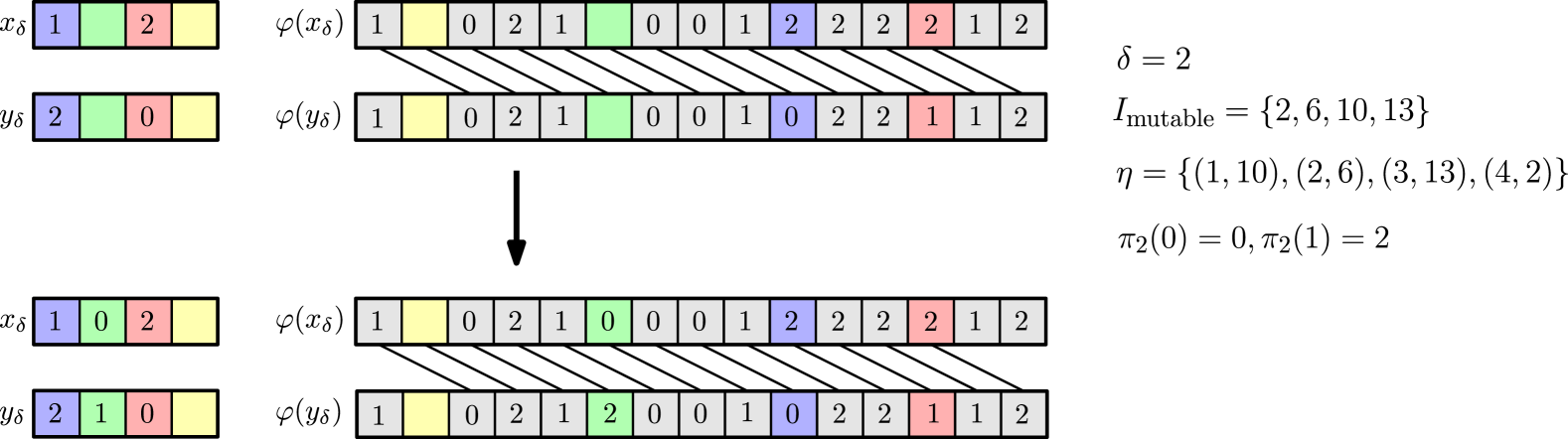
Figure 11: $\eta$ is indicated by the matching colors. The red and purple symbols were set in previous iterations, and we now seek to set the green symbols. Specifically, we require the green symbol of $\varphi(x_{\delta})$ to be 0, while the green symbol of $\varphi(y_{\delta})$ must differ from that of $\varphi(x_{\delta})$. This can be achieved by appropriately setting the green symbols in $x_{\delta}$ and $y_{\delta}$.

We are now ready to describe the collection $\mathcal{C}$ alluded to earlier — it consists of all triples of the form $(x_{\delta},y_{\delta},\mathcal{A}_{\delta})$, where $\delta\in S_{\textnormal{shifts}}$. Let $\tilde{\delta}$ be a uniformly random element of $S_{\textnormal{shifts}}$. The main step in the proof involves bounding the expected cost of $\mathcal{A}_{\tilde{\delta}}$ with respect to $\varphi(x_{\tilde{\delta}})$ and $\varphi(y_{\tilde{\delta}})$.

Lemma 11.2.

$\operatorname*{\mathbb{E}}\left[\textnormal{{cost}}_{\varphi(x_{\tilde{\delta}})}^{\varphi(y_{\tilde{\delta}})}\left(\mathcal{A}_{\tilde{\delta}}\right)\right]<n$, for sufficiently large values of $n$.

Proof.

For ease of notation, define $X:=\varphi(x_{\tilde{\delta}})$, $Y:=\varphi(y_{\tilde{\delta}})$, and $\mathcal{A}:=\mathcal{A}_{\tilde{\delta}}$. Furthermore, define $\varepsilon:=\frac{1}{16|\Sigma|}-\rho$ so that the rate of $\varphi$ is $\frac{1}{2}-\varepsilon$. We will bound $\operatorname*{\mathbb{E}}[\textnormal{{cost}}_{X}^{Y}(\mathcal{A})]$ by individually bounding the expected number of insertions, deletions and substitutions. Bounding the first two is easy — no matter what $\tilde{\delta}$ is, the numbers of insertions or deletions are both always at most $(\Delta-1)$. For substitutions, note that for any $i\in I_{\textnormal{mutable}}$, $X[i]$ is by definition never substituted by $\mathcal{A}$ — it is either matched or deleted. Therefore, in order to bound the expected number of substitutions, it suffices to only focus on the frozen symbols. Let us define an index $i\in I_{\textnormal{frozen}}$ to be good if there exists $j\in I_{\textnormal{frozen}}$ such that $(i,j)\in\mathcal{A}$ and $X[i]=Y[j]$. Less formally, a good index is where a match occurs between a pair of frozen symbols. Let $I_{\textnormal{good}}\subseteq I_{\textnormal{frozen}}$ be the set of all good indices. Clearly, the number of substitutions is upper bounded by $|I_{\textnormal{frozen}}|-|I_{\textnormal{good}}|$. Since $\varphi$ has rate $\frac{1}{2}-\varepsilon$, $|I_{\textnormal{frozen}}|=N\left(\frac{1}{2}+\varepsilon\right)$, and we have —

$$\operatorname*{\mathbb{E}}\left[\textnormal{{cost}}_{X}^{Y}(\mathcal{A})\right]\leq 2(\Delta-1)+N\left(\frac{1}{2}+\varepsilon\right)-\operatorname*{\mathbb{E}}\left[|I_{\textnormal{good}}|\right]$$

Let $\mathbb{1}_{I_{\textnormal{good}}}:I_{\textnormal{frozen}}\to\{0,1\}$ be the indicator function of $I_{\textnormal{good}}\subseteq I_{\textnormal{frozen}}$. By linearity of expectation, we have —

$$\operatorname*{\mathbb{E}}\left[|I_{\textnormal{good}}|\right]=\sum_{i\in I_{\textnormal{frozen}}}\mathbb{1}_{I_{\textnormal{good}}}(i)=\sum_{i\in I_{\textnormal{frozen}}}\Pr[i\in I_{\textnormal{good}}]$$

So, we need to obtain a lower bound on the probability that an index is good. To do so, we partition $X$ and $Y$ into contiguous length-$\Delta$ substrings. For each $t\in[\frac{N}{\Delta}]$ and $\sigma\in\Sigma$, we define $c_{t,\sigma}$ to be the number of times symbol $\sigma$ appears as a frozen symbol in the $t^{\textnormal{th}}$ substring in this partition, i.e.,

$$c_{t,\sigma}:=\left|\{i\in[t(\Delta-1),t\Delta]:i\in I_{\textnormal{frozen}}\textnormal{ and }X[i]=Y[i]=\sigma\}\right|$$

Next we make the following observation.

Observation 11.3.

Let $i\in I_{\textnormal{frozen}}$ and let $t\in[\frac{N}{\Delta}]$ be such that $i\in[t(\Delta-1),t\Delta]$. Then we have —

$$\Pr[i\in I_{\textnormal{good}}]\geq\frac{1}{2}\cdot\frac{c_{t,X[i]}-1}{\Delta-1}$$

Proof.

We have —

$$\Pr[i\in I_{\textnormal{good}}] \geq\Pr\left[\left(i+\tilde{\delta}\in[t(\Delta-1),t\Delta]\right)\wedge\left(\left(i+\tilde{\delta}\in I_{\textnormal{frozen}}\right)\wedge\left(X[i]=Y[i+\tilde{\delta}]\right)\right)\right]$$

$$=\Pr\left[i+\tilde{\delta}\in[t(\Delta-1),t\Delta]\right]\cdot\Pr\left[\left(i+\tilde{\delta}\in I_{\textnormal{frozen}}\right)\wedge\left(X[i]=Y[i+\tilde{\delta}]\right)\middle|i+\tilde{\delta}\in[t(\Delta-1),t\Delta]\right]$$

$$=\frac{1}{2}\cdot\frac{c_{t,X[i]}-1}{\Delta-1}\qed$$

So, we can write —

$$\operatorname*{\mathbb{E}}\left[|I_{\textnormal{good}}|\right]\geq\frac{1}{2(\Delta-1)}\sum_{{t\in\left[\frac{N}{\Delta}\right]}}\sum_{{{\sigma\in\Sigma}}}c_{t,\sigma}(c_{t,\sigma}-1)$$ (10)

The right hand side of (10) is minimized when $c_{t,\sigma}$’s are all the same and equal to $\frac{N(\frac{1}{2}+\varepsilon)}{\frac{N|\Sigma|}{\Delta}}=\frac{\Delta(\frac{1}{2}+\varepsilon)}{|\Sigma|}$. Furthermore, each $c_{t,\sigma}$ can be replaced with $\frac{\Delta}{2|\Sigma|}$ to obtain a value that is strictly smaller than the minimum value of the right hand side of (10). Thus, we have —

$$\operatorname*{\mathbb{E}}\left[|I_{\textnormal{good}}|\right] \geq\frac{1}{2(\Delta-1)}\sum_{{t\in\left[\frac{N}{\Delta}\right]}}\sum_{{{\sigma\in\Sigma}}}c_{t,\sigma}(c_{t,\sigma}-1)$$

$$>\frac{1}{2(\Delta-1)}\cdot\frac{N}{\Delta}\cdot|\Sigma|\cdot\frac{\Delta}{2|\Sigma|}\left(\frac{\Delta}{2|\Sigma|}-1\right)$$

$$\geq\frac{1}{2\Delta}\cdot\frac{N}{2}\left(\frac{\Delta}{2|\Sigma|}-1\right)$$

$$=N\left(\frac{1}{8|\Sigma|}-\frac{1}{4\Delta}\right),$$

and thus, we have —

$$\operatorname*{\mathbb{E}}\left[\textnormal{{cost}}_{X}^{Y}(\mathcal{A})\right]<2(\Delta-1)+N\left(\frac{1}{2}+\varepsilon\right)-N\left(\frac{1}{8|\Sigma|}-\frac{1}{4\Delta}\right)$$

. Consequently, we have —

$$\allowdisplaybreaks n-\operatorname*{\mathbb{E}}\left[\textnormal{{cost}}_{X}^{Y}(\mathcal{A})\right] >n-2(\Delta-1)+N\left(\frac{1}{2}+\varepsilon\right)-N\left(\frac{1}{8|\Sigma|}-\frac{1}{4\Delta}\right)$$

$$=N\left(\frac{1}{2}-\varepsilon\right)-2(\Delta-1)+N\left(\frac{1}{2}+\varepsilon\right)-N\left(\frac{1}{8|\Sigma|}-\frac{1}{4\Delta}\right)$$

$$=N\left(-2\varepsilon+\frac{1}{8|\Sigma|}-\frac{1}{4\Delta}\right)+2(\Delta-1)$$

Now recall that we had $\varepsilon=\frac{1}{16|\Sigma|}-\rho$. Thus, if we choose $\Delta$ to be large enough such that $\frac{1}{8\Delta}<\rho$, we will have $\varepsilon<\frac{1}{16|\Sigma|}-\frac{1}{8\Delta}$ and,

$$n-\operatorname*{\mathbb{E}}\left[\textnormal{{cost}}_{X}^{Y}(\mathcal{A})\right]>\alpha N+2(\Delta-1),$$ (11)

where $\alpha:=-2\varepsilon+\frac{1}{8|\Sigma|}-\frac{1}{4\Delta}>0$. Finally, we note that by making $n$ and, consequently, $N$ sufficiently large, one can make the right-hand side of (11) positive. The conclusion then follows. ∎

Lemma 11.2 guarantees the existence of a triple $(x_{\delta},y_{\delta},\mathcal{A}_{\delta})\in\mathcal{C}$ such that $\textnormal{{cost}}_{\varphi(x_{\delta})}^{\varphi(y_{\delta})}(\mathcal{A}_{\delta})<\Delta_{\textnormal{{Hamming}}}(x_{\delta},y_{\delta})$. However, this contradicts the assumption that $\varphi$ is an isometric embedding of the Hamming metric into the edit metric. ∎

We can further use Theorem 11.1 to immediately get an upper bound on the rate on any $1$-embedding.

Theorem 11.4.

For every alphabet $\Sigma$, there exists an integer $n_{0}$ such that every $1$-embedding $\varphi:\Sigma^{n}\to\Sigma^{N}$ of the Hamming metric into the edit metric with $n\geq n_{0}$ must have rate at most $\frac{1}{2}$.

Proof.

If $\varphi$ is an isometric embedding than Theorem 11.1 implies a rate strictly less than $\frac{1}{2}$. It remains to prove the statement for the case where $\varphi$ is a non-isometric $1$-embedding with $\Delta_{\textnormal{{edit}}}~(\varphi(x),~\varphi(y))=K~\cdot~\Delta_{\textnormal{{Hamming}}}(x,y)$, for all $x,y\in\{0,1\}^{n}$ for some $K$ not equal to $1$. For two strings $x^{\prime},y^{\prime}$ with Hamming distance $1$ we have that $\Delta_{\textnormal{{edit}}}~(\varphi(x^{\prime}),~\varphi(y^{\prime}))=K$ and therefore $K$ must be a positive integer and therefore at least two. The rate $n/N$ of $\varphi$ is furthermore at most $1/K$ because for any two strings $x^{\prime\prime},y^{\prime\prime}$ of maximal Hamming distance $n$ it holds that $N\geq\Delta_{\textnormal{{edit}}}~(\varphi(x^{\prime\prime}),~\varphi(y^{\prime\prime}))=K\cdot n$. This shows that the rate of $\varphi$ is at most $\frac{1}{2}$.

∎

12 Breaking the Rate Barrier via Larger Output Alphabets

Up to this point, we have only considered embeddings where the input and output alphabets have the same size. Theorem 11.1 tells us that in this setting, the rate is necessarily bounded away from $\frac{1}{2}$. While this is the most natural setting, one can also consider embeddings with different-sized input and output alphabets. It turns out that by expanding the output alphabet, it is possible to find isometric embeddings with rates arbitrarily close to 1! However, before explaining how this is done, we must first refine the definition of rate for such embeddings. In the case where the input and output alphabets are of equal size, the rate is defined as the ratio of the input string’s length to the output string’s length. When using a larger output alphabet, the appropriate measure to consider instead is not length but the number of bits.

Definition 12.1.

The rate of any map $\varphi:\Sigma_{\textnormal{in}}\to\Sigma_{\textnormal{out}}$ is the ratio $\frac{n\log|\Sigma_{\textnormal{in}}|}{N\log|\Sigma_{\textnormal{out}}|}$.

Recall the naive embedding from Section 2.1, which inserts a new symbol after each input bit. For that embedding, we have $N=2n$, $\Sigma_{\text{in}}=\{0,1\}$, and $\Sigma_{\text{out}}=\{0,1,\dots,n+1\}$. Thus, even though $\frac{n}{N}$ is as large as $\frac{1}{2}$, the rate, as defined in Definition 12.1, is actually only $\Theta(\frac{1}{\log n})$.

We are now ready to state the main result of this section.

Theorem 12.2.

For every $\rho>0$, there exist alphabets $\Sigma_{\textnormal{in}}$, $\Sigma_{\textnormal{out}}$ and a family of functions $\varphi_{n}:\Sigma_{\textnormal{in}}^{n}\to\Sigma_{\textnormal{out}}^{N}$ for each positive integer $n$ such that the following hold.

1. For every $n$, $\varphi_{n}$ is an isometric embedding of the Hamming metric into the edit metric, i.e., for all $x,y\in\Sigma_{\textnormal{in}}^{n}$, we have $\Delta_{\textnormal{{edit}}}(\varphi_{n}(x),\varphi_{n}(y))=\Delta_{\textnormal{{Hamming}}}(x,y)$.

2. The rate of $\varphi_{n}$ is at least $(1-\rho)$.

Before we prove Theorem 12.2, we first make the following observation about locally self-matching strings.

Observation 12.3.

Let $w$ be an $\varepsilon$-locally self matching string. Then for every substring $s$ of $w$, we have:

$$\Delta_{\widetilde{\textnormal{{edit}}}}(s,s)\geq(1-\varepsilon)|s|$$

Proof.

Let $\mathcal{A}$ be an optimal nowhere-vertical edit distance alignment between $s$ and itself. We have:

$$\Delta_{\widetilde{\textnormal{{edit}}}}(s,s)=\textnormal{{cost}}_{s}^{s}(\mathcal{A})\geq|S_{s}^{s}(\mathcal{A})|+|D_{s}^{s}(\mathcal{A})|\geq|s|-\widetilde{\textnormal{{LCS}}}(s,s)\geq(1-\varepsilon)|s|\qed$$

Proof of Theorem 12.2.

Fix any $\rho>0$. Define $m:=\left\lceil\frac{C(1-\rho)+1}{\rho}\right\rceil$, where $C\geq 1$ is a constant to be chosen later. Furthermore, let $\varepsilon:=\frac{1}{m}$ and $\varepsilon^{\prime}=\frac{\varepsilon}{2}$. We will choose $\Sigma_{\textnormal{in}}=\left[2^{\frac{1}{\varepsilon}\log(\frac{1}{\varepsilon})}\right]$ as our input alphabet. For our output alphabet, we choose $\Sigma_{\textnormal{out}}=\Sigma_{\textnormal{in}}\times\Sigma^{\prime}$, where $\Sigma^{\prime}:=\left[\frac{5e^{2}}{\varepsilon^{\prime 2}}\right]$.

Fix any positive integer $n$ and define $N:=n+\left\lfloor\frac{n}{m-1}\right\rfloor$. Our embedding map $\varphi_{n}:\Sigma_{\textnormal{in}}^{n}\to\Sigma_{\textnormal{out}}^{N}$ is defined as follows. First, we fix some $\varepsilon^{\prime}$-locally self-matching string $w$ of length $N$ over the alphabet $\Sigma^{\prime}$. Since $\varepsilon^{\prime}\leq\frac{1}{2}$, by Theorem 5.2, such a string $w$ always exists. We also fix some arbitrary symbol $\sigma\in\Sigma_{\textnormal{in}}$. Next, given any $x\in\Sigma_{\textnormal{in}}^{n}$, we construct $x_{\textnormal{padded}}\in\Sigma_{\textnormal{in}}^{N}$ by inserting the symbol $\sigma$ after every $(m-1)$ symbols in $x$. Finally, we define $\varphi_{n}(x)\in\Sigma_{\textnormal{out}}^{N}$ to be the product of the strings $x_{\textnormal{padded}}$ and $w$. In other words, we define:

$$\varphi_{n}(x):=(x_{\textnormal{padded}}[1],w[1])\circ(x_{\textnormal{padded}}[2],w[2])\circ\cdots\circ(x_{\textnormal{padded}}[N],w[N])$$

We first claim that if $C$ is appropriately chosen, then $\varphi_{n}$ indeed has rate at least $1-\rho$.

Claim 12.4.

If $C\geq 10$, then the rate of $\varphi_{n}$ is at least $1-\rho$.

Proof.

First note that $N=n+\left\lfloor\frac{n}{m-1}\right\rfloor\leq\frac{nm}{m-1}=\frac{n}{1-\varepsilon}$. Therefore, $\frac{n}{N}\geq 1-\varepsilon$. Furthermore, since $C\geq 1$ and $\rho<1$, $m=\left\lceil\frac{C(1-\rho)+1)}{\rho}\right\rceil\geq 2$. Consequently, $\varepsilon\leq\frac{1}{2}$ and we have $\log|\Sigma^{\prime}|=\log\left(\frac{5e^{2}}{\varepsilon^{\prime 2}}\right)=\log(20e^{2})+2\log\left(\frac{1}{\varepsilon}\right)\leq C\log\left(\frac{1}{\varepsilon}\right)$ for all $\varepsilon\leq\frac{1}{2}$ if $C\geq 10$. Therefore, the rate of $\varphi_{n}$ is:

$$\frac{n\log|\Sigma_{\textnormal{in}}|}{N\log|\Sigma_{\textnormal{out}}|} =\frac{n}{N}\cdot\frac{\log|\Sigma_{\textnormal{in}}|}{\log|\Sigma_{\textnormal{in}}|+\log|\Sigma^{\prime}|}$$

$$\geq(1-\varepsilon)\cdot\frac{\log\left(2^{\frac{1}{\varepsilon}\log\left(\frac{1}{\varepsilon}\right)}\right)}{\log\left(2^{\frac{1}{\varepsilon}\log\left(\frac{1}{\varepsilon}\right)}\right)+C\log\left(\frac{1}{\varepsilon}\right)}$$

$$=(1-\varepsilon)\cdot\frac{\frac{1}{\varepsilon}\log\left(\frac{1}{\varepsilon}\right)}{\frac{1}{\varepsilon}\log\left(\frac{1}{\varepsilon}\right)+C\log\left(\frac{1}{\varepsilon}\right)}$$

$$=\frac{1-\varepsilon}{1+C\varepsilon}$$

$$=1-\frac{(C+1)\varepsilon}{1+C\varepsilon}$$

Now recall that $\varepsilon\leq\frac{\rho}{C(1-\rho)+1}$, and so, $\rho\geq\frac{(C+1)\varepsilon}{1+C\varepsilon}$. The conclusion then follows. ∎

Next, we show that $\varphi_{n}$ is indeed isometric for every positive integer $n$. Suppose not; then there exists a positive integer $n$ and $x,y\in\Sigma_{\textnormal{in}}^{n}$ such that $\Delta_{\textnormal{{edit}}}(\varphi_{n}(x),\varphi_{n}(y))<\Delta_{\textnormal{{Hamming}}}(x,y)$. Let $X:=\varphi_{n}(x)$, $Y:=\varphi_{n}(y)$, and $\mathcal{A}$ be any optimal edit distance alignment between $X$ and $Y$. Since $\Delta_{\textnormal{{Hamming}}}(x,y)=\Delta_{\textnormal{{Hamming}}}(X,Y)$, by assumption, we have $\textnormal{{cost}}(\mathcal{A})<\Delta_{\textnormal{{Hamming}}}(X,Y)$. Similar to the proof of Theorem 6.1, consider the partition of $[N]$ into alternating maximal vertical and maximal nowhere-vertical intervals under $\mathcal{A}$. By the same argument as in the proof of Theorem 6.1, there must exist a nowhere vertical interval $I$ in this partition such that $\textnormal{{cost}}(\mathcal{A}_{|I})<\Delta_{\textnormal{{Hamming}}}(X_{|I},Y_{|I})$. We first note that $|I|\geq\frac{2}{\varepsilon}$. Suppose not. Then since $w$ is a $\frac{\varepsilon}{2}$-locally self-matching string, our construction forces $w_{|I}$ to have all distinct symbols. In this case, we have:

$$\textnormal{{cost}}(\mathcal{A}_{|I})\geq\Delta_{\widetilde{\textnormal{{edit}}}}(X_{|I},Y_{|I})\geq\Delta_{\widetilde{\textnormal{{edit}}}}(w_{|I},w_{|I})=|I|+2>\Delta_{\textnormal{{Hamming}}}(X_{|I},Y_{|I}).$$

Therefore, we may assume that $|I|\geq\frac{2}{\varepsilon}$. But for any $|I|\geq\frac{2}{\varepsilon}$, we have $(1-\frac{\varepsilon}{2})|I|\geq(1-\varepsilon)|I|+1$. And since in $X$ and $Y$, every $(\frac{1}{\varepsilon})^{\text{th}}$ symbol is the same, $(1-\varepsilon)|I|+1$ is an upper bound on $\Delta_{\textnormal{{Hamming}}}(X_{|I},Y_{|I})$. Combining all this, we have:

$$\textnormal{{cost}}(\mathcal{A}_{|I})\geq\Delta_{\widetilde{\textnormal{{edit}}}}(X_{|I},Y_{|I})\geq\Delta_{\widetilde{\textnormal{{edit}}}}(w_{|I},w_{|I})\geq\left(1-\frac{\varepsilon}{2}\right)|I|\geq(1-\varepsilon)|I|+1\geq\Delta_{\textnormal{{Hamming}}}(X_{|I},Y_{|I}),$$

which is a contradiction. ∎

Acknowledgments

Part of the work of Sudatta Bhattacharya, Sanjana Dey, Elazar Goldenberg and Michal Koucký was carried out during a visit to DIMACS, with support from the National Science Foundation under grant number CCF-1836666. Sudatta Bhattacharya and Michal Koucký were partially supported by the Grant Agency of the Czech Republic under the grant agreement no. 24-10306S and by Charles Univ. project UNCE 24/SCI/008. Mursalin Habib, Bernhard Haeupler, and Karthik C. S. were partially funded by the Ministry of Education and Science of Bulgaria’s support for INSAIT as part of the Bulgarian National Roadmap for Research Infrastructure. Bernhard Haeupler was partially funded through the European Research Council (ERC) under the European Union’s Horizon 2020 research and innovation program (ERC grant agreement 949272). Elazar Goldenberg, Mursalin Habib, and Karthik C. S. were partially supported by the National Science Foundation Grant CCF-2313372. Mursalin Habib and Karthik C. S. were partially supported by the National Science Foundation Grant CCF-2443697 and a grant from the Simons Foundation, Grant Number 825876, Awardee Thu D. Nguyen. Sanjana Dey was partially supported by the Fonds de la Recherche Scientifique – FNRS under Grant n° T.0188.23 (PDR ControlleRS).

Appendix A Searching for a Misaligner

In this section, we give a high-level description of our program used to discover the $(320,676,8,0.1625)$-misaligner from Lemma 8.1. The naive way of building the collection of strings or codewords would involve starting with three randomly generated codewords satisfying Properties 1 and 2. Then, at each iteration, a candidate string satisfying Property 1 would be generated and tested against the remaining properties. Note that Property 2 is easy to check and can be done efficiently. Property 4 can also be checked naively. Even Property 3b can be afforded to be checked naively because we only need to take every pair of strings and compare them with the new string. The most costly property is 3a, where we need to test the new string $s$ exhaustively against every triple of strings $c_{1},c_{2},c_{3}$ already in the collection – verifying that the edit distance between $s$ and every substring of $c_{1}\circ c_{2}\circ c_{3}$ (where a prefix of $s$ aligns with a suffix of $c_{1}$, a middle portion of $s$ with $c_{2}$, and a suffix of $s$ with a prefix of $c_{3}$) meets the required bound. This approach becomes prohibitively slow, especially because Property 3a requires checking many such alignments. To address this, we need to adopt a more efficient strategy.

In contrast to the naive approach, our scheme in ced-320.cpp builds a collection that is guaranteed to satisfy Property 3a (while ignoring the other properties). Instead of testing a new string $s$ against every possible triple $(c_{1},c_{2},c_{3})$, the program first performs an extensive preprocessing phase. It generates a large number of random strings and computes their pairwise edit distances—focusing separately on the prefix of one string with every other entire string, and the suffix of one string with every other entire string, and also for every possible middle portion of one string with every other entire string. These computations are accumulated into statistical tables. Pstat stores the number of pairs of strings with a certain edit distance when the prefix of one is compared to the other string. Similarly, Sstat and Mstat record the corresponding statistics for suffixes and middle sections, respectively. Then, for each possible length of suffix, prefix, or middle section, thresholds are computed as the typical values derived from the stored statistics. By determining the edit distance thresholds (stored in arrays like Pthr, Sthr, and Mthr) corresponding to a very small violation rate (controlled by the parameter RANKFRAC), the program creates a set of “filters” that a candidate string must pass.

Now, to build the collection, every new candidate string $c$ is checked again against every string $c^{\prime}$ already in the collection: the edit distance of every prefix of $c$ with the entire $c^{\prime}$, the edit distance of every suffix of $c$ with the entire $c^{\prime}$, and the edit distance of every possible middle substring of $c$ with the entire $c^{\prime}$ are verified against the corresponding thresholds. We also check the thresholds for $c$ and $c^{\prime}$ interchanged. If any of them is violated, then $c$ isn’t added to the collection. In this way, for every string $c$ in the final collection, every other string is acceptable when aligning any prefix, suffix, or middle portion of $c$ with it. This precisely captures condition 3a, which requires that when a string $c$ is aligned against the concatenation of three other strings $c_{1},c_{2},c_{3}$ (with a prefix of $c$ aligned to $c_{1}$, a middle portion to $c_{2}$, and a suffix to $c_{3}$), all such alignments satisfy the specified edit distance thresholds.

This preprocessing-based filtering dramatically reduces the computational load and allows ced-320.cpp to efficiently generate an initial collection where every string satisfies Property 3a. Note that the most computationally heavy step is to check Property 3a, so we optimized this step by performing extensive preprocessing to compute statistical thresholds that serve as fast filters. This optimization avoids the need for an exhaustive check of every candidate string against every possible triple of existing strings. The rest of the properties are checked naively using the code in ted-320.cpp. This code checks whether each of the properties is satisfied, and if it is not satisfied it suggests strings that should be removed from the collection to satisfy a given property.

Appendix B Explicit Bounds for Synchronization Strings on Alphabets of Size Four

In this section, we prove Corollary 1.8, which states that there exists a $0.999606$-synchronization string over an alphabet of size four. To do so, we first need the following definition.

Definition B.1.

A string $w$ of length $n$ is called an $\varepsilon$-weak synchronization string if for all $1\leq i<j<k\leq n$ such that $k-i\geq\frac{1}{1-\varepsilon}$, we have $\Delta_{\textnormal{{edit}}}\left(w_{|[i,j-1]},w_{|[j,k-1]}\right)\geq(1-\varepsilon)(k-i)$.

Lemma B.2.

There exists an infinite 0.995268-weak synchronization string over the binary alphabet.

Proof.

By Theorem 6.3 in [CHL⁺19], if $\varepsilon^{\prime}$-synchronization strings exist over an alphabet of $2^{k}$, then $\varepsilon$-weak synchronization strings exist over an binary alphabet, where $\varepsilon:=1-\frac{1-\varepsilon^{\prime}}{18k}$. Furthermore, every $\frac{\varepsilon}{2}$-locally self-matching string is an $\varepsilon$-synchronization string (Theorem 6.4 in [HS21b]). Thus by Theorem 5.2 and finding the minimum value of the expression

$$1-\frac{1-\frac{\varepsilon^{\prime}}{2}}{18\log_{2}\left(\frac{4e^{2}}{\varepsilon^{\prime 2}}\cdot\left(1+4\sqrt[4]{\frac{\varepsilon^{\prime}}{2}}\right)\right)}$$

as $\varepsilon^{\prime}$ ranges in $\left(0,\frac{1}{2}\right]$, one gets the desired conclusion. ∎

We also make use of the following lemma.

Lemma B.3.

Given an infinite $\varepsilon$-weak synchronization string over a binary alphabet, one can construct an infinite $\frac{\varepsilon+11}{12}$-synchronization string over an alphabet of size four.

Proof.

This follows directly from Theorem 6.4 in [CHL⁺19]. ∎

Now Lemmas B.2 and B.3 together imply Corollary 1.8.

References

- [ABC+23] Amir Abboud, MohammadHossein Bateni, Vincent Cohen-Addad, Karthik C. S., and Saeed Seddighin. On complexity of 1-center in various metrics. In Nicole Megow and Adam D. Smith, editors, Approximation, Randomization, and Combinatorial Optimization. Algorithms and Techniques, APPROX/RANDOM 2023, September 11-13, 2023, Atlanta, Georgia, USA, volume 275 of LIPIcs, pages 1:1–1:19. Schloss Dagstuhl - Leibniz-Zentrum für Informatik, 2023.
- [BI18] Arturs Backurs and Piotr Indyk. Edit distance cannot be computed in strongly subquadratic time (unless SETH is false). SIAM J. Comput., 47(3):1087–1097, 2018.
- [CGK16] Diptarka Chakraborty, Elazar Goldenberg, and Michal Koucký. Streaming algorithms for embedding and computing edit distance in the low distance regime. In Daniel Wichs and Yishay Mansour, editors, Proceedings of the 48th Annual ACM SIGACT Symposium on Theory of Computing, STOC 2016, Cambridge, MA, USA, June 18-21, 2016, pages 712–725. ACM, 2016.
- [CHL+19] Kuan Cheng, Bernhard Haeupler, Xin Li, Amirbehshad Shahrasbi, and Ke Wu. Synchronization strings: Highly efficient deterministic constructions over small alphabets. In Proceedings of the ACM-SIAM Symposium on Discrete Algorithms (SODA), pages 2185–2204, 2019.
- [CKL22] Vincent Cohen-Addad, Karthik C. S., and Euiwoong Lee. Johnson coverage hypothesis: Inapproximability of k-means and k-median in lp-metrics. In Joseph (Seffi) Naor and Niv Buchbinder, editors, Proceedings of the 2022 ACM-SIAM Symposium on Discrete Algorithms, SODA 2022, Virtual Conference / Alexandria, VA, USA, January 9 - 12, 2022, pages 1493–1530. SIAM, 2022.
- [Cod] Github repository. https://anonymous.4open.science/r/ham-to-edit-11D8.
- [FGK24] Henry L. Fleischmann, Surya Teja Gavva, and Karthik C. S. On approximability of steiner tree in lp-metrics. In David P. Woodruff, editor, Proceedings of the 2024 ACM-SIAM Symposium on Discrete Algorithms, SODA 2024, Alexandria, VA, USA, January 7-10, 2024, pages 1669–1703. SIAM, 2024.
- [GXTL10] Xinbo Gao, Bing Xiao, Dacheng Tao, and Xuelong Li. A survey of graph edit distance. Pattern Analysis and applications, 13:113–129, 2010.
- [HS18] Bernhard Haeupler and Amirbehshad Shahrasbi. Synchronization strings: Explicit constructions, local decoding, and applications. In Proceedings of the ACM Symposium on Theory of Computing (STOC), pages 841–854, 2018.
- [HS21a] Bernhard Haeupler and Amirbehshad Shahrasbi. Synchronization strings and codes for insertions and deletions - a survey. CoRR, abs/2101.00711, 2021.
- [HS21b] Bernhard Haeupler and Amirbehshad Shahrasbi. Synchronization strings: Codes for insertions and deletions approaching the singleton bound. J. ACM, 68(5):36:1–36:39, 2021.
- [HSS18] Bernhard Haeupler, Amirbehshad Shahrasbi, and Madhu Sudan. Synchronization strings: List decoding for insertions and deletions. In Proceedings of the International Conference on Automata, Languages, and Programming (ICALP), 2018.
- [HSV18] Bernhard Haeupler, Amirbehshad Shahrasbi, and Ellen Vitercik. Synchronization strings: Channel simulations and interactive coding for insertions and deletions. In Proceedings of the International Conference on Automata, Languages, and Programming (ICALP), pages 75:1–75:14, 2018.
- [Jow12] Hossein Jowhari. Efficient communication protocols for deciding edit distance. In Leah Epstein and Paolo Ferragina, editors, Algorithms - ESA 2012 - 20th Annual European Symposium, Ljubljana, Slovenia, September 10-12, 2012. Proceedings, volume 7501 of Lecture Notes in Computer Science, pages 648–658. Springer, 2012.
- [KM20] Karthik C. S. and Pasin Manurangsi. On closest pair in euclidean metric: Monochromatic is as hard as bichromatic. Combinatorica, 40(4):539–573, 2020.
- [KR09] Robert Krauthgamer and Yuval Rabani. Improved lower bounds for embeddings into . SIAM J. Comput., 38(6):2487–2498, 2009.
- [LLL+16] Anders Liljas, Lars Liljas, Goran Lindblom, Poul Nissen, Morten Kjeldgaard, and Miriam-rose Ash. Textbook of structural biology, volume 8. World Scientific, 2016.
- [LMW02] Ming Li, Bin Ma, and Lusheng Wang. On the closest string and substring problems. Journal of the ACM, 49, 03 2002.
- [MT10] Robin A Moser and Gábor Tardos. A constructive proof of the general lovász local lemma. Journal of the ACM (JACM), 57(2):1–15, 2010.
- [MV93] Andres Marzal and Enrique Vidal. Computation of normalized edit distance and applications. IEEE transactions on pattern analysis and machine intelligence, 15(9):926–932, 1993.
- [Nav01] Gonzalo Navarro. A guided tour to approximate string matching. ACM computing surveys (CSUR), 33(1):31–88, 2001.
- [NCB] National Center for Biotechnology Information homepage. https://www.ncbi.nlm.nih.gov/. Accessed: 2024-11-04.
- [NR05] François Nicolas and Eric Rivals. Hardness results for the center and median string problems under the weighted and unweighted edit distances. Journal of Discrete Algorithms, 3(2):390–415, 2005. Combinatorial Pattern Matching (CPM) Special Issue.
- [OR07] Rafail Ostrovsky and Yuval Rabani. Low distortion embeddings for edit distance. J. ACM, 54(5):23, 2007.
- [Rub18] Aviad Rubinstein. Hardness of approximate nearest neighbor search. In Ilias Diakonikolas, David Kempe, and Monika Henzinger, editors, Proceedings of the 50th Annual ACM SIGACT Symposium on Theory of Computing, STOC 2018, Los Angeles, CA, USA, June 25-29, 2018, pages 1260–1268. ACM, 2018.
- [SZ99] Leonard J Schulman and David Zuckerman. Asymptotically good codes correcting insertions, deletions, and transpositions. IEEE transactions on information theory, 45(7):2552–2557, 1999.
- [WF74] Robert A. Wagner and Michael J. Fischer. The string-to-string correction problem. J. ACM, 21(1):168–173, January 1974.