A Polynomial-Time Algorithm for Variational Inequalities under the Minty Condition

Abstract

Solving (Stampacchia) variational inequalities (SVIs) is a foundational problem at the heart of optimization, with a host of critical applications ranging from engineering to economics. However, this expressivity comes at the cost of computational hardness. As a result, most research has focused on carving out specific subclasses that elude those intractability barriers. A classical property that goes back to the 1960s is the Minty condition, which postulates that the Minty VI (MVI) problem—the weak dual of the SVI problem—admits a solution.

In this paper, we establish the first polynomial-time algorithm—that is, with complexity growing polynomially in the dimension $d$ and $\log(1/\epsilon)$—for solving $\epsilon$-SVIs for Lipschitz continuous mappings under the Minty condition. Prior approaches either incurred an exponentially worse dependence on $1/\epsilon$ (and other natural parameters of the problem) or made overly restrictive assumptions—such as strong monotonicity. To do so, we introduce a new variant of the ellipsoid algorithm wherein separating hyperplanes are obtained after taking a gradient descent step from the center of the ellipsoid. It succeeds even though the set of SVIs can be nonconvex and not fully dimensional. Moreover, when our algorithm is applied to an instance with no MVI solution and fails to identify an SVI solution, it produces a succinct certificate of MVI infeasibility. We also show that deciding whether the Minty condition holds is $\mathsf{coNP}$-complete, thereby establishing that the disjunction of those two problems—computing $\epsilon$-SVIs and ascertaining MVI infeasibility—is polynomial-time solvable even though each problem is individually intractable.

We provide several extensions and new applications of our main results. Specifically, we obtain the first polynomial-time algorithms for i) solving monotone VIs, ii) globally minimizing a (potentially nonsmooth) quasar-convex function, and iii) computing Nash equilibria in multi-player harmonic games. Finally, in two-player general-sum concave games, we give the first polynomial-time algorithm that outputs either a Nash equilibrium or a strict coarse correlated equilibrium.

1 Introduction

Variational inequalities (VIs) are a mainstay framework at the heart of optimization that unifies a host of foundational problems in diverse areas ranging from engineering to economics [Kinderlehrer and Stampacchia, 2000, Facchinei and Pang, 2003, Bensoussan and Lions, 2011]. The basic problem underpinning VIs—when restricted to Euclidean spaces—can be formulated as follows.

Definition 1.1 (SVIs).

Let ${\mathcal{X}}$ be a convex and compact subset of $\mathbb{R}^{d}$ and a (single-valued) mapping $F:{\mathcal{X}}\to\mathbb{R}^{d}$. The $\epsilon$-approximate Stampacchia variational inequality (SVI) problem asks for a point ${\bm{x}}\in{\mathcal{X}}$ such that

$$\langle F({\bm{x}}),{\bm{x}}^{\prime}-{\bm{x}}\rangle\geq-\epsilon\quad\forall{\bm{x}}^{\prime}\in{\mathcal{X}}.$$ (1)

Assuming $F$ is continuous, an exact SVI solution (that is, with $\epsilon=0$) always exists [Facchinei and Pang, 2003]—by Brouwer’s fixed-point theorem applied on the function ${\bm{x}}\mapsto\Pi_{{\mathcal{X}}}({\bm{x}}-\eta F({\bm{x}}))$, where $\Pi_{\mathcal{X}}$ is the (Euclidean) projection mapping. For computational purposes, we have introduced a slackness $\epsilon>0$ in the right-hand side of (1); without this relaxation, the only SVI solution can be irrational. It is assumed that $\epsilon$ is given (in binary) as part of the input, and the goal is to design algorithms with complexity growing polynomially in $\log(1/\epsilon)$ and the dimension $d$.

A canonical example of Definition 1.1 is the problem of computing fixed points of gradient descent in constrained optimization. In particular, for a differentiable function $f$, the $\epsilon$-SVI problem corresponding to $F:=\nabla f$ can be expressed as $\langle\nabla f({\bm{x}}),{\bm{x}}^{\prime}-{\bm{x}}\rangle\geq-\epsilon$ for all ${\bm{x}}^{\prime}\in{\mathcal{X}}$, which captures precisely the first-order optimality conditions [Boyd and Vandenberghe, 2004]. Another standard example of Definition 1.1 is the problem of computing (approximate) Nash equilibria in multi-player games [Nash, 1950].

Unfortunately, by virtue of encompassing (approximate) Nash equilibria, solving general SVIs is computationally intractable—namely, $\PPAD$-hard [Papadimitriou, 1994]—even when $F$ is linear and $\epsilon$ is an absolute constant [Rubinstein, 2015]; recent work by Bernasconi et al. [2024], Kapron and Samieefar [2024] characterizes the exact complexity of SVIs, as well as generalizations thereof. In fact, even in the special case discussed above wherein $F:=\nabla f$, computing $\epsilon$-SVI solutions is also hard—under certain well-believed complexity assumptions—when $\epsilon$ is exponentially small in the dimension [Fearnley et al., 2023].

In light of the intractability of solving general SVIs, most research has restricted its attention to more structured classes of problems. Following a long and burgeoning line of work that goes back to the 1960s, we operate under the Minty condition (introduced below as 1.3); it is based on a variant of SVIs (Definition 1.1) tracing back to Minty [1967], known as the Minty VI problem.

Definition 1.2 (MVIs).

Let ${\mathcal{X}}$ be a convex and compact subset of $\mathbb{R}^{d}$ and a mapping $F:{\mathcal{X}}\to\mathbb{R}^{d}$. The Minty variational inequality (MVI) problem asks for a point ${\bm{x}}\in{\mathcal{X}}$ such that

$$\langle F({\bm{x}}^{\prime}),{\bm{x}}^{\prime}-{\bm{x}}\rangle\geq 0\quad\forall{\bm{x}}^{\prime}\in{\mathcal{X}}.$$ (2)

Unlike SVIs, an MVI solution may not exist even when $F$ is continuous—indeed, the Minty condition is precisely the requirement that an MVI solution exists:

Assumption 1.3 (Minty condition).

A variational inequality problem $\textsc{VI}({\mathcal{X}},F)$ satisfies the Minty condition if there exists ${\bm{x}}\in{\mathcal{X}}$ that satisfies (2).

Assuming continuity, Definition 1.2 refines Definition 1.1 in the following sense.

Lemma 1.4 (Minty’s lemma).

If $F$ is continuous and ${\mathcal{X}}$ is convex and compact, then any MVI solution is also an SVI solution.

On the other hand, an SVI solution need not be an MVI solution—otherwise 1.3 would always hold under a continuous mapping. One well-known special case in which the set of MVI solutions does coincide with the set of SVI solutions is when $F$ is monotone; that is, when $\langle F({\bm{x}})-F({\bm{x}}^{\prime}),{\bm{x}}-{\bm{x}}^{\prime}\rangle\geq 0$ for all ${\bm{x}},{\bm{x}}^{\prime}\in{\mathcal{X}}$. This holds more generally when $F$ is pseudomonotone, which means that $\langle F({\bm{x}}^{\prime}),{\bm{x}}-{\bm{x}}^{\prime}\rangle\geq 0\implies\langle F({\bm{x}}),{\bm{x}}-{\bm{x}}^{\prime}\rangle\geq 0$ for all ${\bm{x}},{\bm{x}}^{\prime}\in{\mathcal{X}}$. Importantly, the Minty condition is more permissive than monotonicity, encompassing a broader class of problems; indeed, it captures a host of nonconvex optimization problems (cf. Section 3).

By now, it is well-known that under the Minty condition, there are algorithms with complexity scaling polynomially in $1/\epsilon$ (and all other natural parameters of the problem) for computing an $\epsilon$-SVI solution. This goes back to the early, pioneering work of Sibony [1970], Martinet [1970], and Korpelevich [1976]; in particular, the latter showed that the extra-gradient method converges in all monotone VIs—this stands in stark contrast to the usual gradient descent algorithm, which can cycle even in two-player zero-sum games [Mertikopoulos et al., 2018b], which are monotone. Motivated by many applications in machine learning and reinforcement learning, there has been renewed interest in the Minty condition recently (e.g., Burachik and Millan, 2020, Lei and He, 2021, Lin and Jordan, 2024, Song et al., 2020, Ye, 2022, Mertikopoulos and Zhou, 2019, Mertikopoulos et al., 2018a, Daskalakis et al., 2020, Patris and Panageas, 2024, Cai et al., 2024b). However, those existing results become vacuous when $\epsilon$ is exponentially small in terms of the dimension $d$. On the other end of the spectrum, all existing algorithms with $\poly(d,\log(1/\epsilon))$ complexity make restrictive assumptions that are significantly stronger than the Minty condition, akin to strong monotonicity or some type of an “error bound” (for example, we refer to Song et al., 2020, Ye, 2022, Lüthi, 1985, Magnanti and Perakis, 1995, discussed further in Section 1.2).

1.1 Our results

Table 1: Summary of main results. All algorithms (upper bounds) have runtimes that depend polynomially on both $d$ and $\log(1/\epsilon)$, and, to our knowledge, are the first algorithms for their respective settings with this dependence. ^†: Unlike our other positive results, our result for quasar-convex optimization holds even when $F=\nabla f$ is not Lipschitz continuous.

	Result	Reference
Upper bounds	•  $\epsilon$-SVIs under the Minty condition	Theorem 1.5
	•  $\epsilon$-MVIs under a monotone $F$	Corollary 1.6
	•  $\epsilon$-SVIs or $\Omega_{\epsilon}(\epsilon^{2})$-strict EVIs	Theorem 1.8
	•  $\epsilon$-global optimization under quasar-convexity†	Theorem 1.11
	•  $\epsilon$-Nash equilibria in harmonic games	Corollary 1.12
	•  $\epsilon$-Nash or $\Omega_{\epsilon}(\epsilon^{4})$-strict CCEs in two-player concave games	Theorem 1.13
Lower bounds	•  Deciding MVI feasibility (i.e., Minty condition)	Theorem 1.14
	•  Solving MVIs under the Minty condition	Proposition 1.16

We establish the first polynomial-time algorithm for solving $\epsilon$-SVIs under the Minty condition. In what follows, we assume that the constraint set ${\mathcal{X}}$ is accessed through a (weak) separation oracle (Definition 2.3) and ${\mathcal{B}}_{1}(\bm{0})\subseteq{\mathcal{X}}\subseteq{\mathcal{B}}_{R}(\bm{0})$ for some $R\leq\poly(d)$; the latter can be met be bringing ${\mathcal{X}}$ into isotropic position, a transformation that does not affect our main result (as formalized in Appendix A). With regard to the mapping $F$, we assume that it can be evaluated in polynomial time, it is $L$-Lipschitz continuous, and $\|F({\bm{x}})\|$ is bounded by $B>0$ (2.5). We are now ready to state our main result.

Theorem 1.5 (Precise version in Theorem 4.7).

Under the Minty condition (1.3), there is an algorithm that runs in $\poly(d,\log(B/\epsilon),\log L)$ time and returns an $\epsilon$-SVI solution.

Compared to all previous results cited earlier under the Minty condition, this result improves exponentially the dependence on $1/\epsilon$ and $L$. We clarify that, although the underlying algorithm posits the Minty condition, its execution does not hinge on knowing an MVI solution. Indeed, a peculiar feature of Theorem 1.5 is that while its main precondition concerns MVIs, the output itself is an approximate SVI solution; the reason for this discrepancy will become clear shortly.

Furthermore, Theorem 1.5 implies the first, to our knowledge, polynomial-time algorithm for solving monotone VIs—perhaps the most well-studied structural assumption in the literature.

Corollary 1.6.

When $F$ is monotone, there is an algorithm that runs in $\poly(d,\log(B/\epsilon),\log L)$ time and returns an $\epsilon$-MVI solution.

Indeed, as we saw earlier, monotonicity implies that the set of MVI solutions coincides with the set of SVI solutions, so Corollary 1.6 directly follows from Theorem 1.5. Before we present some more results that build on Theorem 1.5 (gathered in Table 1), we dive into our technical approach.

1.1.1 Technical approach: proof of Theorem 1.5

The proof of Theorem 1.5 relies on the usual (central-cut) ellipsoid algorithm, but with certain unusual twists.

Challenge 1: lack of convexity

The first immediate conundrum lies in the fact that the set of SVI solutions is generally not convex even when the Minty condition holds. By contrast, the set of MVI solutions is convex, thereby being a better candidate on which to execute ellipsoid. But this approach also runs into an apparent difficulty: while a point ${\bm{x}}\in{\mathcal{X}}$ can be confirmed to be an $\epsilon$-SVI solution by invoking a (linear) optimization oracle, this is not so for MVIs. Indeed, as we show in this paper (Section 1.1.4), ascertaining MVI membership is -complete.

In summary, the set of SVI solutions admits an efficient membership oracle, while the set of MVI solutions is convex. A natural approach now presents itself: execute the ellipsoid with respect to the set of MVIs, but only verify SVI membership. To do so, the first key idea is this: if a point ${\bm{x}}\in{\mathcal{X}}$ is not an $\epsilon$-SVI solution, then $F({\bm{x}})$ yields a hyperplane separating ${\bm{x}}$ from the set of MVIs. As a result, this allows us to run the ellipsoid algorithm with respect to the convex set of MVI solutions, with the peculiarity that we only test for SVI membership during the execution of the algorithm. So long as the algorithm fails to identify an approximate SVI solution, the volume of the ellipsoid shrinks geometrically.

Challenge 2: lack of full dimensionality

This now brings us to the next key challenge: the set of MVI solutions is generally not fully dimensional. It is therefore unclear whether the volume of the ellipsoid can be used as a yardstick to measure the progress of the algorithm. There is a standard approach for addressing this issue, at least for rational polyderal sets (for example, Grötschel et al., 1993, Chapter 6): restrict the execution of the ellipsoid to suitable subspaces whenever one of the ellipsoid’s axis gets too small. However, this standard approach falls short in our problem; we provide a concrete numerical example in Section 6.3 illustrating that the usual ellipsoid algorithm fails to identify $\epsilon$-SVI solutions.

To address this problem, we introduce a new algorithmic idea. Namely, we show that we can produce, in polynomial time, what we refer to as a strict separating hyperplane; this key ingredient underpinning Theorem 1.5 is summarized below (the precise version is Lemma 4.5). (Technically, we need to allow ${\bm{a}}$ to be approximately in ${\mathcal{X}}$ since we are dealing with general convex sets—in accordance with Lemma B.2—but we do not dwell on this issue in the introduction.)

Lemma 1.7 (SVI membership or MVI strict separation).

Given a point ${\bm{a}}\in{\mathcal{X}}\cap\mathbb{Q}^{d}$ and $\epsilon\in\mathbb{Q}_{>0}$, there is a polynomial-time algorithm that either

1. ascertains that $\bm{a}$ is an $\epsilon$-SVI solution or

2. returns $\bm{c}\in\mathbb{Q}^{d}$, with $\|\bm{c}\|_{\infty}=1$, such that $\langle\bm{c},{\bm{x}}\rangle\leq\langle\bm{c},{\bm{a}}\rangle-\gamma$ for any point ${\bm{x}}\in{\mathcal{X}}$ that satisfies the Minty VI (2), where $\gamma=\epsilon^{2}\cdot\poly(R^{-1},L^{-1},B^{-1})$.

Figure 1: One step of our ellipsoid algorithm—when the current ellipsoid center ${\bm{a}}^{(t)}$ is not already an $\epsilon$-SVI solution. While $F({\bm{a}}^{(t)})$ separates ${\bm{a}}^{(t)}$ from the set of MVI solutions (in this case a single point), $F(\tilde{{\bm{a}}}^{(t)})$ yields a $\gamma$-strict separating hyperplane, which turns out to be crucial; see Section 6.3.

To obtain a hyperplane that strictly separates ${\bm{a}}\in{\mathcal{X}}$ from the set of MVI solutions (in the sense of Item 2), assuming that ${\bm{a}}$ is not an $\epsilon$-SVI solution, we perform a gradient descent step starting from ${\bm{a}}$. Since ${\bm{a}}$ is not an $\epsilon$-SVI solution, it can be shown that the resulting point, say $\tilde{{\bm{a}}}\in{\mathcal{X}}$, is such that $F(\tilde{{\bm{a}}})$ strictly separates ${\bm{a}}$ from the set of MVIs (Lemma 4.5); this is illustrated in Figure 1.

Interestingly, this simple algorithmic maneuver is, at least conceptually, similar to the extra-gradient method [Korpelevich, 1976] (and variants thereof), which is known to converge—albeit at an inferior rate that grows polynomially in $1/\epsilon$—under the Minty condition. Accordingly, we call the overall algorithm ExtraGradientEllipsoid (Algorithm 2); it is an incarnation of the central-cut ellipsoid endowed with additional gradient descent steps. We stress again that this step cannot be avoided: the usual ellipsoid algorithm without the extra-gradient step fails (Section 6.3) due to its inability to generate strict separating hyperplanes. This phenomenon mirrors the behavior of first-order methods, whereby regular gradient descent fails to converge to an SVI solution—even in monotone problems—whereas the extra-gradient method succeeds [Korpelevich, 1976]. As such, we find that there is an intriguing analogy between the behavior we uncover for ellipsoid-based algorithms and what has been known for decades pertaining to gradient-based algorithms.

To finish the proof of Theorem 1.5, we observe that Lemma 1.7—and in particular the sequence of strict separating hyperplanes produced during the execution of the ellipsoid—implies that the volume of the ellipsoid cannot shrink too much (Lemma 4.6). Indeed, since the ellipsoid always contains the set of MVI solutions, and the separating hyperplanes are strict, every MVI solution is in some sense far from the boundary of the ellipsoid, which in turn implies that the ellipsoid must have nontrivial volume. In other words, the algorithm will necessarily terminate with an $\epsilon$-SVI solution, as promised—so long as an MVI solution exists.

If no MVI solution exists, the above algorithm might fail, that is, the volume may end up shrinking too much. But in this case, as we shall see, a small adaptation to ExtraGradientEllipsoid can produce a polynomial certificate of MVI infeasibility (cf. Theorem 1.8).

1.1.2 A certificate of MVI infeasibility

We now treat the general setting in which the Minty condition can be altogether violated. Our next result shows how to employ ExtraGradientEllipsoid so as to produce a certificate of MVI infeasibility. But how does such a “certificate” look like?

To answer this, we rely on the recently introduced concept of expected VIs (EVIs) (Definition 3.6). This is a relaxation of Definition 1.1 that only imposes the SVI constraint in expectation for points draw from a distribution. For readers familiar with equilibrium concepts in game theory, it is instructive to have in mind that EVIs are to SVIs what (average) coarse correlated equilibria (ACCEs) (Definition 3.8) are to Nash equilibria. The key point is that there is a strong duality between MVIs and EVIs (Proposition 3.7); namely, the Minty condition holds if and only if no EVI solution with negative gap exists—we refer to the latter object as a strict EVI solution. In other words, the mere existence of a strict EVI exposes MVI infeasibility. This brings us to the following key refinement of Theorem 1.5.

Theorem 1.8 (SVI or strict EVI; precise version in Theorem 4.16).

There is an algorithm that runs in $\poly(d,\log(B/\epsilon),\log L)$ time and returns either

1. an $\epsilon$-SVI solution or

2. an $\Omega_{\epsilon}(\epsilon^{2})$-strict EVI solution.

This clearly strengthens Theorem 1.5: under the Minty condition no strict EVIs exist, so Item 2 in Theorem 1.8 will never arise under 1.3. A key reference point here is a result by Anagnostides et al. [2022b], who provided an algorithm with a similar output guarantee, but with complexity scaling polynomially—rather than logarithmically—in $1/\epsilon$; as such, Theorem 1.8 yields again an exponential improvement over existing results.

The proof of Theorem 1.8 is based on an application of duality between MVIs and EVIs. In particular, the minimax theorem implies that, once the volume of the ellipsoid becomes sufficiently small, there is a distribution supported on $\tilde{{\bm{a}}}^{(1)},\dots,\tilde{{\bm{a}}}^{(T)}$ that is a $\gamma/2$-strict EVI, where $\gamma$ is the strictness parameter per Lemma 1.7 and $\tilde{{\bm{a}}}^{(t)}$ is obtained after a gradient descent step starting from the center of the ellispoid at the $t$th iteration (Figure 1); coupled with Lemma 1.7, this explains the $\Omega_{\epsilon}(\gamma)=\Omega_{\epsilon}(\epsilon^{2})$ strictness in Item 2. We are thus left with the simple problem of optimizing the mixing weights of a distribution with a polynomial support. This algorithmic maneuver closely resembles the celebrated “ellipsoid against hope” algorithm of Papadimitriou and Roughgarden [2008] (cf. Jiang and Leyton-Brown, 2011, Farina and Pipis, 2024, Daskalakis et al., 2025), which is also based on running ellipsoid on an infeasible program.

A strict EVI, besides certifying MVI infeasibility, is an interesting object in its own right. It is, by definition, a solution concept with negative gap, thereby being particularly stable—any possible deviation is not just suboptimal, but significantly so. Indeed, its incarnation in the context of games has been already used to address the equilibrium selection problem, as we explain more in Section 1.2. Furthermore, in certain applications, the EVI gap translates to a performance guarantee in terms of some underlying objective function; the smoothness framework of Roughgarden [2015]—and its extension for general VI problems given in Definition 3.3—is a prime example of this in the context of multi-player games. It turns out that an EVI with a negative gap yields a strict improvement over the bound predicted by the smoothness framework.

But there is something more that is especially notable about Theorem 1.8: each of the computational problems in Items 1 and 2 is computationally hard on its own, yet Theorem 1.8 shows that their disjunction is easy! In particular, computing $\epsilon$-SVI solutions is a well-known -complete problem. With regard to strict EVIs, we provide a characterization of its complexity in this paper, establishing $\NP$-completeness (Theorem 1.14). To put this into context, we highlight that there has been interest in characterizing the complexity of the union of two problems, especially in the realm of $\TFNP$. A notable contribution here is the work of Daskalakis and Papadimitriou [2011] that examined the complexity of problems in $\PPAD\cap\PLS$, where $\PLS$ stands for “polynomial local search” [Johnson et al., 1988]. They observed that if a problem A is $\PPAD$-complete and B is $\PLS$-complete, then the problem that must return either a solution to A or to B is $\PPAD\cap\PLS$-complete—that is, $\CLS$-complete [Fearnley et al., 2023]; unlike Theorem 1.8, this observation by Daskalakis and Papadimitriou [2011] assumes that A and B are defined with respect to different instances. In this context, Theorem 1.8 provides an example in which the disjunction of two hard problems—one -complete and the other -complete—defined with respect to the same instance is easy.

1.1.3 Implications and extensions

Moving forward, we discuss several important consequences and extensions of our main results for optimization and game theory.

Quasar-convex optimization

The first implication concerns optimizing quasar-convex functions; this is a relaxation of convexity that has attracted significant interest recently (for example, Fu et al., 2023, Hinder et al., 2020, Caramanis et al., 2024, Hardt et al., 2018, Gower et al., 2021, Danilova et al., 2022, Wang and Wibisono, 2023).

Definition 1.9 (Quasar-convexity).

Let $\lambda\in(0,1]$ and ${\bm{x}}$ be a minimizer of a differentiable function $f:{\mathcal{X}}\to\mathbb{R}$. We say that $f$ is $\lambda$-quasar-convex with respect to ${\bm{x}}$ if

$$f({\bm{x}})\geq f({\bm{x}}^{\prime})+\frac{1}{\lambda}\langle\nabla f({\bm{x}}^{\prime}),{\bm{x}}-{\bm{x}}^{\prime}\rangle\quad\forall{\bm{x}}^{\prime}\in{\mathcal{X}}.$$ (3)

(We elaborate more on how this relates to other properties in Section 3.1.) Not only does $\textsc{VI}({\mathcal{X}},\nabla f)$ (under Definition 1.9) satisfy the Minty condition, but every approximate SVI solution is also an approximate global minimum of $f$ (Proposition 3.2); combined with Theorem 1.5, we obtain the first polynomial-time algorithm for globally minimizing smooth quasar-convex functions.

Corollary 1.10.

There is a $\poly(d,\log(B/\epsilon),\log(1/\lambda),\log L)$-time algorithm that outputs a point ${\bm{x}}\in{\mathcal{X}}$ such that $f({\bm{x}})\leq\min_{{\bm{x}}^{\prime}\in{\mathcal{X}}}f({\bm{x}}^{\prime})+\epsilon$ for any $\lambda$-quasar-convex function $f$.

This result can be generalized (cf. Proposition 3.5) by considering a broader class of VI problems (Definition 3.3), beyond quasar-convex functions. Interestingly, this class of problems encompasses (a special case of) smooth games, famously introduced by Roughgarden [2015]; we explain this in more detail in Section 3.1.

Furthermore, as we shall now see, Corollary 1.10 can be significantly strengthened by relaxing the assumption that $\nabla f$ is continuous (Theorem 1.11). This follows a long line of research in nonsmooth optimization (e.g., Zhang et al., 2020, Davis et al., 2022, Tian et al., 2022, Jordan et al., 2023). In this context, we show that under quasar-convexity—and, more generally, its extension based on Definition 3.3—it is possible to entirely eliminate the (logarithmic) dependence on $L$.

Theorem 1.11 (Precise version in Theorem 4.15).

There is a $\poly(d,\log(B/\epsilon),\log(1/\lambda))$-time algorithm that outputs a point ${\bm{x}}\in{\mathcal{X}}$ such that $f({\bm{x}})\leq\min_{{\bm{x}}^{\prime}\in{\mathcal{X}}}f({\bm{x}}^{\prime})+\epsilon$ for any $\lambda$-quasar-convex function $f$.

(Since we are considering additive approximations, a dependence on $B$ is necessary since one can always rescale $f$.) The key idea here is that quasar-convexity yields a strict separating hyperplane without requiring an extra-gradient step, which is where the Lipschitz continuity of $F$ came into play in Lemma 1.7. Theorem 1.11 should be compared with the result of Lee and Valiant [2016] pertaining to optimizing star-convex functions—the special case of Definition 1.9 where $\lambda=1$.

Weak Minty condition

We also strengthen Theorem 1.5 along another axis. Perhaps the most immediate question is how far can one relax the assumption that $\textsc{VI}({\mathcal{X}},F)$ satisfies the Minty condition—while accepting the fact that, in light of the intractability of general VIs, imposing some assumptions is inevitable. Naturally, this question has received ample attention in contemporary research (cf. Section 4.3). One permissive condition that has emerged from that line of work is the weak Minty property put forward by Diakonikolas et al. [2021] in the unconstrained setting. In Definition 4.10, we introduce a natural version of that notion for the constrained setting. And we show, in Theorem 4.13, that Theorem 1.5 can be applied in a certain regime of the weak Minty condition.

Harmonic games

We next discuss two implications and extensions of our main results for game theory. The first concerns harmonic games (Definition 3.13), a class of multi-player games at the heart of the seminal decomposition of Candogan et al. [2011], covered in more detail in Section 3.3. Leveraging Theorem 1.5, we obtain the first polynomial-time algorithm for computing $\epsilon$-Nash equilibria (per Definition 3.9, captured by $\epsilon$-SVIs) in multi-player harmonic games under the polynomial expectation property [Papadimitriou and Roughgarden, 2008]; this latter condition postulates that one can efficiently compute utility gradients (equivalently, the underlying mapping $F$ can be evaluated efficiently), which holds in most succinct classes of games.

Corollary 1.12.

There is a polynomial-time algorithm for computing $\epsilon$-Nash equilibria in (succinct) multi-player harmonic games under the polynomial expectation property.

This algorithm is based on the observation that harmonic games satisfy a weighted version of the Minty condition. In particular, after applying a suitable transformation, we show that the induced VI problem satisfies the usual Minty condition under a Lipschitz continuous mapping (Proposition 3.15), at which point Corollary 1.12 follows from Theorem 1.5. Crucial to this argument is the fact that the weights in harmonic games cannot be too close to $0$ (Lemma 3.14), for otherwise the Lipschitz continuity parameter would blow up; this issue is the crux in our refinement for two-player games, which is the subject of the next paragraph.

Nash or strict coarse correlated equilibria in two-player games

Our next application concerns equilibrium computation in two-player concave games. As we alluded to, EVIs are closely related to the notion of a coarse correlated equilibrium (CCE) from game theory. More precisely, when the underlying VI problem corresponds to a multi-player game, the EVI gap equates to the sum of the players’ deviation benefits under a correlated distribution; this does not quite capture the usual notion of a CCE in which one bounds the maximum of the deviation benefits (Section 3.2). In light of this, we also provide the following refinement of Theorem 1.8 in two-player concave games.

Theorem 1.13 (Precise version in Theorem 5.2).

In a two-player concave game, there is an algorithm that runs in time $\poly(d,\log(B/\epsilon),\log L)$ and returns either

1. an $\epsilon$-Nash equilibrium or

2. an $\Omega_{\epsilon}(\epsilon^{4})$-strict CCE.

Unlike Theorem 1.8, which can be applied to multi-player games to find Nash or strict ACCEs, Theorem 5.2 cannot be extended to games with more than two players—one can always include a third player who always obtains zero utility. Theorem 1.13 provides an exponential improvement over a known result by Anagnostides et al. [2022a], who gave a $\poly(d,B,L,1/\epsilon)$-time algorithm for the same problem via optimistic mirror descent.

As in harmonic games, the proof of Theorem 1.13 is based on analyzing a weighted version of the Minty condition—this allows transitioning from the sum to the maximum deviation benefit. But, unlike harmonic games, here we need to handle the case where one of the weights is arbitrarily close to $0$, in which case the Lipschitz continuity parameter blows up, which in turn neutralizes the strict separation oracle of Lemma 1.7. We address this by providing a tailored separation oracle for two-player games when one of the weights gets too close to $0$ (Lemma 5.4).

1.1.4 Lower bounds

As promised, we complement Theorem 1.8 by proving that determining whether the Minty condition holds is $\coNP$-complete.

Theorem 1.14 (Precise version in Propositions 6.2, 6.3 and 6.5).

Determining whether a VI problem satisfies the Minty condition (1.3) is $\coNP$-complete. Hardness holds even for two-player concave games or multi-player (succinct) normal-form games and even when a constant approximation error $\epsilon$ is allowed.

Inclusion in $\coNP$ follows because a strict EVI solution is itself an efficiently verifiable witness of MVI infeasibility. On the other hand, for explicitly represented (normal-form) games, the duality between EVIs and MVIs (Proposition 3.7) enables us to show the following positive result.

Proposition 1.15.

There is a polynomial-time algorithm that determines whether an explicitly represented (normal-form) game satisfies the Minty condition.

In particular, for such problems, it is well-known that one can efficiently optimize over the polytope of EVI solutions, so one can in particular minimize the equilibrium gap.

One final natural question that arises from Theorem 1.5 concerns the complexity of computing Minty VI solutions (per Definition 1.2), when promised that such a solution exists; by Lemma 1.4, this would be stronger than computing SVI solutions. With a straightforward construction, we observe that this is information-theoretically impossible.

Proposition 1.16 (Precise version in Propositions 6.8 and 6.10).

Computing an $\epsilon$-MVI solution requires $\Omega(1/\epsilon)$ oracle evaluations to $F$ even when an MVI solution is guaranteed to exist and $d=1$. When $d$ is large, it requires $\Omega(2^{d})$ oracle evaluations even when $\epsilon$ is an absolute constant.

In particular, this lower bound implies that the dependence on $\lambda$ in Theorems 1.11 and 1.10 cannot be removed (Proposition 6.8).

1.2 Further related work

We have already provided references establishing $\poly(d,1/\epsilon)$-time algorithms (ignoring the dependency on other parameters of the problem) for solving $\epsilon$-SVIs under the Minty condition. Here, it is worth elaborating more on the prior results with complexity scaling polynomially in $\log(1/\epsilon)$; the upshot is that they all rest on restrictive assumptions that are significantly stronger than the Minty condition. Lüthi [1985] gave an algorithm for $\epsilon$-SVIs using the ellipsoid, but the analysis assumes that $F$ is strongly monotone. As we have seen, the Minty condition is weaker than the assumption that $F$ is monotone, while strong monotonicity is a significantly stronger assumption still. Aghassi et al. [2006] derive a compact convex formulation for a class of SVIs that includes monotone, affine VIs over polyhedral sets (cf. Harker and Xiao, 1991). Magnanti and Perakis [1995] established a polynomial-time algorithm for SVIs under what is today referred to as $\alpha$-cocoercivity: $\langle F({\bm{x}})-F({\bm{x}}^{\prime}),{\bm{x}}-{\bm{x}}^{\prime}\rangle\geq\alpha\|F({\bm{x}})-F({\bm{x}}^{\prime})\|^{2}$ for all ${\bm{x}},{\bm{x}}^{\prime}\in{\mathcal{X}}$, where $\alpha>0$. Relatedly, Goffin et al. [1997] provide a nonasymptotic analysis for a cutting-plane method under the assumption that $F$ is pseudo-cocoercive—that is, $\langle F({\bm{x}}^{\prime}),{\bm{x}}-{\bm{x}}^{\prime}\rangle\geq 0\implies\langle F({\bm{x}}),{\bm{x}}-{\bm{x}}^{\prime}\rangle\geq\alpha\|F({\bm{x}})-F({\bm{x}}^{\prime})\|^{2}$ for all ${\bm{x}},{\bm{x}}^{\prime}\in{\mathcal{X}}$. Song et al. [2020] provided an algorithm with complexity scaling as $O_{\epsilon}(\log(1/\epsilon))$ under a strengthening of the Minty condition. Linear convergence was also established by Ye [2022] under a certain “error bound,” which is again significantly stronger than the Minty condition.

The Minty variational inequality problem also relates to the seminal concept of an evolutionary stable strategy (ESS) from evolutionary game theory [Smith and Price, 1973]. We refer to Migot and Cojocaru [2021] for precise connections between MVIs and ESSs; the upshot is that a point ${\bm{x}}\in{\mathcal{X}}$ that satisfies the MVI strictly for any ${\bm{x}}^{\prime}\neq{\bm{x}}$ equates to a certain variant of ESS. Interestingly, Conitzer [2019] showed that even ascertaining the existence of an ESS in two-player (normal-form) games is $\SigmaP$-complete; by contrast, Proposition 3.10 shows that determining whether the Minty property holds in games with a constant number of players can be solved in polynomial time. From a computational standpoint, this makes the Minty condition a more compelling criterion for ascertaining evolutionary plausibility.

Recent research has focused extensively on higher-order methods for computing SVIs [Bullins and Lai, 2022, Huang et al., 2022, Adil et al., 2022, Huang and Zhang, 2022, Jiang and Mokhtari, 2022, Lin and Jordan, 2024]. For example, Lin and Jordan [2024] developed an algorithm with iteration complexity scaling with $O_{\epsilon}(\epsilon^{-2/(p+1)})$; the main caveat with those results is that implementing each iteration requires time that grows exponentially in $p$.

Moreover, computing the strictest (A)CCE has been used to address the equilibrium selection problem [Marris et al., 2025]; a game can have multiple CCEs of varying properties, so it is often not clear which one is to be preferred from either a prescriptive or descriptive point of view. The (A)CCE that minimizes the equilibrium gap—which can be negative (cf. Proposition 3.7)—offers one possible answer to that dilemma.

For further references pertaining to earlier developments on variational inequalities, we refer to the survey of Harker and Pang [1990].

2 Preliminaries

Before moving on, we lay out some basic notation and background on optimization, and then proceed to formally state our blanket assumptions.

Notation

We use lowercase boldface letters, such as ${\bm{x}}$, to denote points in $\mathbb{R}^{d}$ and capital letters, such as $\mathbf{A}\in\mathbb{R}^{d\times d^{\prime}}$, for matrices. The $j$th coordinate of ${\bm{x}}$ is accessed by ${\bm{x}}[j]$. For ${\bm{x}}\in\mathbb{R}^{d}$ and ${\bm{x}}^{\prime}\in\mathbb{R}^{d^{\prime}}$, $({\bm{x}},{\bm{x}}^{\prime})\in\mathbb{R}^{d+d^{\prime}}$ represents their concatenation. We denote by $\operatorname{\mathsf{size}}(r)$ the encoding length of a rational number $r\in\mathbb{Q}$ in binary. If $\langle\cdot,\cdot\rangle$ represents the standard inner product, $\|{\bm{x}}\|:=\sqrt{\langle{\bm{x}},{\bm{x}}\rangle}$ is the (Euclidean) $\ell_{2}$ norm of ${\bm{x}}$, while $\|{\bm{x}}\|_{\infty}:=\max_{1\leq j\leq d}{\bm{x}}[j]$ is its $\ell_{\infty}$ norm. For a matrix $\mathbf{A}\in\mathbb{R}^{d\times d^{\prime}}$, $\|\mathbf{A}\|$ denotes its spectral norm. $\mathbf{I}_{d}\in\mathbb{R}^{d\times d}$ is the $d\times d$ identity matrix. ${\mathcal{B}}_{r}({\bm{x}})$ is the (closed) Euclidean ball centered at ${\bm{x}}\in\mathbb{R}^{d}$ with radius $r>0$. We use $\Delta(d)$ for the $d$-simplex: $\Delta(d):=\{{\bm{x}}\in\mathbb{R}^{d}_{\geq 0}:\sum_{j=1}^{d}{\bm{x}}[j]=1\}$. We use the notation $O(\cdot),\Theta(\cdot),\Omega(\cdot)$ to suppress absolute constants. We sometimes use $O_{n}(\cdot)$ to highlight the dependence only on the parameter $n$.

We distinguish between a VI problem, denoted by $\textsc{VI}({\mathcal{X}},F)$—which is given by a mapping $F:{\mathcal{X}}\to\mathbb{R}^{d}$ that can be evaluated in polynomial time (2.5) and a constraint set that is implicitly accessed through a (weak) separation oracle (Definition 2.3)—and a solution thereof, be it an SVI (Definition 1.1) or an MVI (Definition 1.2).

Let ${\mathcal{X}}$ be a convex and compact set in $\mathbb{R}^{d}$. We define

$${\mathcal{X}}^{-\epsilon}:=\{{\bm{x}}\in{\mathcal{X}}:{\mathcal{B}}_{\epsilon}({\bm{x}})\subseteq{\mathcal{X}}\},$$ (4)

where we recall that ${\mathcal{B}}_{\epsilon}({\bm{x}})$ is the (closed) Euclidean ball centered at ${\bm{x}}\in\mathbb{R}^{d}$ with radius $\epsilon>0$. (4) describes all points that are “$\epsilon$-deep” inside ${\mathcal{X}}$. Similarly, we define

$${\mathcal{X}}^{+\epsilon}:=\{{\bm{x}}^{\prime}\in\mathbb{R}^{d}:\|{\bm{x}}^{\prime}-{\bm{x}}\|\leq\epsilon\text{ for some }{\bm{x}}\in{\mathcal{X}}\}=\bigcup_{{\bm{x}}\in{\mathcal{X}}}{\mathcal{B}}_{\epsilon}({\bm{x}}),$$ (5)

the set of all points that are “$\epsilon$-close” to ${\mathcal{X}}$. Throughout this paper, we work with a general convex set ${\mathcal{X}}$, which might even be supported solely on irrational points; it will thus be necessary to consider (4) and (5)—in place of ${\mathcal{X}}$—in the definitions that follow to ensure the existence of points with rational coordinates.

We say that ${\mathcal{X}}$ is in isotropic position if for a uniformly sampled ${\bm{x}}\sim{\mathcal{X}}$, we have $\operatorname*{\mathbb{E}}[{\bm{x}}]=0$ and $\operatorname*{\mathbb{E}}[{\bm{x}}{\bm{x}}^{\top}]=\mathbf{I}_{d\times d}$. There is a polynomial-time algorithm that brings any constraint set ${\mathcal{X}}$ into isotropic position (for example, Lovász and Vempala, 2006). This transformation does not affect our main result (Theorem 4.7) or implications thereof (Appendix A), so we assume it without loss of generality. If ${\mathcal{X}}$ is in isotropic position, we can assume that ${\mathcal{B}}_{1}(\bm{0})\subseteq{\mathcal{X}}\subseteq{\mathcal{B}}_{R}(\bm{0})$ for some $R\leq\poly(d)$; in fact, all our positive results apply even when $R\leq\exp(\poly(d))$.

Remark 2.1.

We assume throughout that ${\mathcal{X}}$ is well-bounded, in that ${\mathcal{B}}_{r}(\bm{a})\subseteq{\mathcal{X}}\subseteq{\mathcal{B}}_{R}(\bm{0})$, which in particular implies that ${\mathcal{X}}$ is fully dimensional. Under this assumption, it is known (for example, see Grötschel et al. [1993, Lemma 3.2.35]) that if $\langle\bm{c},{\bm{x}}\rangle\leq\gamma$ holds for all ${\bm{x}}\in{\mathcal{X}}^{-\delta}$, it follows that

$$\langle\bm{c},{\bm{x}}\rangle\leq\gamma+\frac{2R}{r}\|\bm{c}\|\delta\quad\forall{\bm{x}}\in{\mathcal{X}}.$$ (6)

As a result, we can safely consider deviations in ${\mathcal{X}}$, not merely in ${\mathcal{X}}^{-\delta}$, by suitably rescaling the precision parameters—by virtue of (6).

Continuing with some basic geometric definitions, we say that a set ${\mathcal{E}}\subseteq\mathbb{R}^{d}$ is an ellipsoid if there exists a vector $\bm{a}\in\mathbb{R}^{d}$ and a positive definite matrix $\mathbf{A}\in\mathbb{R}^{d\times d}$ such that

$${\mathcal{E}}={\mathcal{E}}(\mathbf{A},\bm{a}):=\{{\bm{x}}\in\mathbb{R}^{d}:\langle{\bm{x}}-\bm{a},\mathbf{A}^{-1}({\bm{x}}-\bm{a})\rangle\leq 1\};$$

above, we use the inverse of $\mathbf{A}$ so as to be consistent with Grötschel et al. [1993]. $\operatorname{vol}({\mathcal{E}})$ is the volume of the ellipsoid ${\mathcal{E}}$.

We are now ready to introduce some basic oracles, which are known to be (polynomial-time) equivalent when ${\mathcal{X}}$ is well-bounded; in light of Remark 2.1, we can handle deviations ${\bm{x}}^{\prime}\in{\mathcal{X}}$ instead of ${\bm{x}}^{\prime}\in{\mathcal{X}}^{-\epsilon}$. The first one simply ascertains (approximate) membership.

Definition 2.2 (Weak membership; Grötschel et al., 1993).

Given a point ${\bm{x}}\in\mathbb{Q}^{d}$ and a rational number $\epsilon\in\mathbb{Q}_{>0}$, decide whether ${\bm{x}}\in{\mathcal{X}}^{+\epsilon}$.

A separation oracle takes a step further: if the point is not (approximately) in the set, it proceeds by producing a separating hyperplane, as defined next.

Definition 2.3 (Weak separation; Grötschel et al., 1993).

Given a point $\bm{x}\in\mathbb{R}^{d}$ and a rational number $\epsilon\in\mathbb{Q}_{>0}$, either

• assert that ${\bm{x}}\in{\mathcal{X}}^{+\epsilon}$ or

• find a vector $\bm{c}\in\mathbb{Q}^{d}$ with $\|\bm{c}\|_{\infty}=1$ such that $\langle\bm{c},{\bm{x}}^{\prime}\rangle<\langle\bm{c},{\bm{x}}\rangle+\epsilon$ for every ${\bm{x}}^{\prime}\in{\mathcal{X}}^{-\epsilon}$.

The final useful oracle (approximately) optimizes linear functions with respect to the constraint set; it enables verifying whether a point is an approximate SVI solution.

Definition 2.4 (Weak optimization; Grötschel et al., 1993).

Given a vector $\bm{c}\in\mathbb{Q}^{d}$ and a rational number $\epsilon\in\mathbb{Q}_{>0}$, either

• assert that ${\mathcal{X}}^{-\epsilon}$ is empty or

• find a vector ${\bm{x}}\in{\mathcal{X}}^{+\epsilon}\cap\mathbb{Q}^{d}$ such that $\langle\bm{c},\bm{x}\rangle\leq\langle\bm{c},{\bm{x}}^{\prime}\rangle+\epsilon$ for all ${\bm{x}}^{\prime}\in{\mathcal{X}}^{-\epsilon}$.

Our main assumption concerning ${\mathcal{X}}$ is that it is given implicitly through access to any of those computationally equivalent oracles.

With regard to the mapping $F$ of the underlying variational inequality problem, we gather our assumptions below; some of our results, such as Theorem 4.15, weaken these assumptions.

Assumption 2.5.

For a fixed $\epsilon_{0}\in\mathbb{Q}_{>0}$, the mapping $F:{\mathcal{X}}^{+\epsilon_{0}}\to\mathbb{R}^{d}$ satisfies the following:

1. for any rational ${\bm{x}}\in{\mathcal{X}}^{+\epsilon_{0}}\cap\mathbb{Q}^{d}$, $F({\bm{x}})$ is a rational number that can be evaluated exactly in $\poly(d)$ time, with $\operatorname{\mathsf{size}}(F({\bm{x}}))\leq\poly(\operatorname{\mathsf{size}}({\bm{x}}))$;

2. for any ${\bm{x}},{\bm{x}}^{\prime}\in{\mathcal{X}}^{+\epsilon_{0}}$, $\|F({\bm{x}})-F({\bm{x}}^{\prime})\|\leq L\|{\bm{x}}-{\bm{x}}^{\prime}\|$ for some $L\in\mathbb{Q}_{>0}$; and

3. for any ${\bm{x}}\in{\mathcal{X}}^{+\epsilon_{0}}$, $\|F({\bm{x}})\|\leq B$ for some $B\in\mathbb{Q}_{>0}$.

Above, we use the parameter $\epsilon_{0}\ll 1$ for convenience in the notation (in Lemma B.2); for the purpose of the main body, $\epsilon_{0}=0$. Regarding Item 1, a weaker assumption, which suffices for our purposes, is that we have access to an oracle that, for any ${\bm{x}}\in{\mathcal{X}}\cap\mathbb{Q}^{d}$ and rational $\delta\in\mathbb{Q}_{>0}$, returns $\bm{g}\in\mathbb{Q}^{d}$ such that $\|F({\bm{x}})-\bm{g}\|\leq\delta$. When specialized to multi-player games, Item 1 is precisely the polynomial expectation property of Papadimitriou and Roughgarden [2008].

For simplicity, our algorithm takes as input $L$ and $B$, under the promise that $F$ satisfies 2.5; this is not necessary: one can run the algorithm starting from $L_{0},B_{0}$; if the output does not satisfy the desired property, it suffices to repeat, setting $L_{1}=2L_{0}$ and $B_{1}=2B_{0}$, and so on.

We next state a simple, well-known result regarding optimizing convex functions with respect to a constraint set that admits a separation oracle.

Theorem 2.6 (Grötschel et al., 1993).

Let ${\mathcal{X}}\subseteq\mathbb{R}^{d}$ be in isotropic position, given by a (weak) separation oracle, and $f:{\mathcal{X}}\to\mathbb{R}$ a convex function that can be evaluated exactly in $\poly(d)$ time. There is a $\poly(d,\log(1/\epsilon))$-time algorithm that outputs ${\bm{x}}\in{\mathcal{X}}^{+\epsilon}$ such that $f({\bm{x}})\leq\min_{{\bm{x}}^{\prime}\in{\mathcal{X}}^{-\epsilon}}f({\bm{x}}^{\prime})+\epsilon$.

Remark 2.7.

In addition, suppose that $f$ is differentiable and $\mu$-strongly convex: $f({\bm{x}})\geq f({\bm{x}}^{\prime})+\langle\nabla f({\bm{x}}^{\prime}),{\bm{x}}-{\bm{x}}^{\prime}\rangle+\frac{\mu}{2}\|{\bm{x}}-{\bm{x}}^{\prime}\|^{2}$. If ${\bm{x}}^{\prime}$ is the global minimum of $f$ with respect to ${\mathcal{X}}^{-\epsilon}$, we have $\|\Pi_{{\mathcal{X}}^{-\epsilon}}({\bm{x}})-{\bm{x}}^{\prime}\|\leq 2\epsilon/\mu+2(f(\Pi_{{\mathcal{X}}^{-\epsilon}}({\bm{x}}))-f({\bm{x}}^{\prime}))/\mu$; if $f$ is Lipschitz continuous, it follows that ${\bm{x}}$ is also geometrically close to ${\bm{x}}^{\prime}$.

3 Consequences and manifestations of the Minty condition

The Minty condition (1.3) is intimately related to several important and seemingly disparate concepts in optimization and game theory. This section gathers a number of such connections, most of which are new. In Section 3.1, we begin by exploring connections in optimization, mostly revolving around quasar-convexity (Definition 1.9) and a more general incarnation thereof in general VI problems (Definition 3.3). Section 3.2 establishes a duality between MVIs and a relaxation of SVIs called expected VIs (Proposition 3.7), which are closely related to the notion of coarse correlated equilibria from game theory. We then leverage this duality to show that in explicitly represented multi-player games, ascertaining whether the Minty condition holds can be phrased as a linear program of polynomial size; this is to be contrasted with our -hardness for succinct games (Theorem 6.5). Section 3.3 examines classes of games that satisfy the Minty condition, which notably includes harmonic games—after applying a suitable transformation (Proposition 3.15).

3.1 Optimization

We first turn our attention to optimizing a single function. Let $f:{\mathcal{X}}\to\mathbb{R}$ be a differentiable function to be minimized. As we discussed earlier, an $\epsilon$-SVI solution ${\bm{x}}\in{\mathcal{X}}$ to the problem arising when $F:=\nabla f({\bm{x}})$ is an approximate stationary point of gradient descent applied on $f$; namely, $\langle\nabla f({\bm{x}}),{\bm{x}}^{\prime}-{\bm{x}}\rangle\geq-\epsilon$ for all ${\bm{x}}^{\prime}\in{\mathcal{X}}$. In particular, if there exists $r>0$ such that ${\mathcal{B}}_{r}({\bm{x}})\subseteq{\mathcal{X}}$—that is, ${\bm{x}}$ is in the interior of ${\mathcal{X}}$—it follows that $\|\nabla f({\bm{x}})\|\leq\epsilon/r$. Of course, when $f$ is nonconvex, $\epsilon$-SVIs are not generally approximate global minima—they can even be saddle points. This is in stark contrast to MVI solutions, although their existence is not guaranteed in general; indeed, the following was observed, for example, by Huang and Zhang [2023, Theorem 2.10].

Proposition 3.1 (Huang and Zhang, 2023).

Consider the optimization problem $\min_{{\bm{x}}\in{\mathcal{X}}}f({\bm{x}})$, where $f$ is differentiable and ${\mathcal{X}}$ is convex and compact. If ${\bm{x}}\in{\mathcal{X}}$ is an MVI solution with respect to $F:=\nabla f$, then ${\bm{x}}$ is a global minimum of $f$.

On the other hand, a global minimum of $f$ is not necessarily an MVI solution—otherwise our main result (Theorem 4.7) would imply $\CLS\subseteq\P$ (cf. Fearnley et al., 2023); see Huang and Zhang [2023, Remark 2.11] for a concrete example.

One special case in which SVI solutions do correspond to global minima is when $f$ is quasar-convex [Fu et al., 2023, Hinder et al., 2020, Caramanis et al., 2024, Hardt et al., 2018], in the following sense (restated from the introduction).

See 1.9

Quasar-convexity is a generalization of the usual notion of convexity: if (3) holds for any ${\bm{x}},{\bm{x}}^{\prime}\in{\mathcal{X}}$ and $\lambda=1$, one recovers precisely convexity for differentiable functions. Further, when (3) holds only with respect to ${\bm{x}}$ (as in Definition 1.9) but with $\lambda=1$, we get the notion of star-convexity [Lee and Valiant, 2016, Nesterov and Polyak, 2006]. It follows immediately from the definition that quasar-convexity is in fact a strengthening of the Minty condition, which further guarantees that all approximate SVI solutions are approximately global minima in terms of value—this latter property does not necessarily hold under solely the Minty condition.

Proposition 3.2.

Let $F:=\nabla f$ for a differentiable, $\lambda$-quasar-convex function $f:{\mathcal{X}}\to\mathbb{R}$ with respect to a global minimum ${\bm{x}}\in{\mathcal{X}}$ of $f$. Then, ${\bm{x}}$ is a solution to the Minty VI problem. Furthermore, any $\epsilon$-SVI solution satisfies $f({\bm{x}}^{\prime})\leq f({\bm{x}})+\epsilon/\lambda$.

Proof.

The fact that ${\bm{x}}$ satisfies the Minty VI follows since

$$\langle\nabla f({\bm{x}}^{\prime}),{\bm{x}}^{\prime}-{\bm{x}}\rangle\geq\lambda(f({\bm{x}}^{\prime})-f({\bm{x}}))\geq 0$$

for any ${\bm{x}}^{\prime}\in{\mathcal{X}}$, where we used the fact that $f({\bm{x}})\leq f({\bm{x}}^{\prime})$ (${\bm{x}}$ is a global minimum of $f$). Now, let ${\bm{x}}^{\prime}$ be an $\epsilon$-SVI solution, which implies that $\langle\nabla f({\bm{x}}^{\prime}),{\bm{x}}-{\bm{x}}^{\prime}\rangle\geq-\epsilon$. Combining with (3), we have

$$f({\bm{x}}^{\prime})\leq f({\bm{x}})+\frac{\epsilon}{\lambda},$$

as promised. ∎

Smooth VIs

The notion of quasar-convexity given in Definition 1.9 can be significantly generalized to general VI problems, as observed recently by Zhang et al. [2025]; as we shall see, this captures a special case of the seminal notion of smoothness, introduced by Roughgarden [2015]. (For convenience, we take the perspective of maximization in the following definition.)

Definition 3.3 (Smoothness for VIs; Zhang et al., 2025).

Let $\lambda>0$ and $\nu>-1$. Consider further a function $Q:{\mathcal{X}}\to\mathbb{R}$ and a global maximum ${\bm{x}}\in{\mathcal{X}}$ of $Q$. A VI problem with respect to the mapping $F:{\mathcal{X}}\to\mathbb{R}^{d}$ is called $(\lambda,\nu)$-smooth with respect to $Q$ and ${\bm{x}}$ if

$$\langle F({\bm{x}}^{\prime}),{\bm{x}}^{\prime}-{\bm{x}}\rangle\geq\lambda Q({\bm{x}})-(\nu+1)Q({\bm{x}}^{\prime})\quad\forall{\bm{x}}^{\prime}\in{\mathcal{X}}.$$ (7)

In particular, $(\lambda,\lambda-1)$-smoothness equates to $\lambda$-quasar-convexity when we define $Q:=-f$ and $F:=\nabla f$. Furthermore, in the special case of multi-player games, Definition 3.3 is equivalent to the seminal concept of smoothness introduced by Roughgarden [2015]—in particular, Definition 3.3 is a direct extension of the more general concept of “local smoothness” per Roughgarden and Schoppmann [2015].

Definition 3.4 (Smoothness for games; Roughgarden, 2015).

Let $\lambda>0$ and $\nu>-1$, and ${\bm{x}}\in\operatorname*{argmax}_{{\bm{x}}^{\prime}\in{\mathcal{X}}}\mathsf{SW}({\bm{x}}^{\prime})$ with respect to an $n$-player game $\Gamma$. $\Gamma$ is called $(\lambda,\nu)$-smooth with respect to ${\bm{x}}$ if

$$\sum_{i=1}^{n}u_{i}({\bm{x}}_{i},{\bm{x}}_{-i}^{\prime})\geq\lambda\mathsf{SW}({\bm{x}})-\nu\mathsf{SW}({\bm{x}}^{\prime})\quad\forall{\bm{x}}^{\prime}\in{\mathcal{X}}.$$ (8)

By defining $Q:=\mathsf{SW}$—the social welfare function, we see that (8) is equivalent to (7) due to multilinearity. The key motivation behind Definition 3.4 is that it enables bounding the social welfare of any (A)CCE in terms of the optimal welfare [Roughgarden, 2015]. Smoothness manifests itself prominently in a host of important applications; for example, we refer to the survey of Roughgarden et al. [2017]. For our purposes, the key point is that Definition 3.3 enables generalizing Proposition 3.2 to a broader family of problems beyond (single-function) optimization:

Proposition 3.5.

Let $\lambda>0$, a function $Q:{\mathcal{X}}\to\mathbb{R}$ with a global maximum at ${\bm{x}}\in{\mathcal{X}}$, and a mapping $F:{\mathcal{X}}\to\mathbb{R}^{d}$. If the corresponding VI problem is $(\lambda,\lambda-1)$-smooth with respect to $Q$ and ${\bm{x}}$, then ${\bm{x}}$ is a solution to the Minty VI problem. Furthermore, any $\epsilon$-SVI solution satisfies $Q({\bm{x}}^{\prime})\leq Q({\bm{x}})+\epsilon/\lambda$.

The proof is analogous to that of Proposition 3.2.

3.2 Expected VIs and duality with MVIs

The next connection is that MVIs are, in a precise sense, duals of a certain relaxation of SVIs recently introduced by Zhang et al. [2025], called expected VIs; we refer to Cai et al. [2024a] and Şeref Ahunbay [2025] for some precursors of that definition in the context of nonconcave games.

We begin by stating the definition of expected VIs; following Zhang et al. [2025], we use the term “expected VIs,” as opposed to expected SVIs, although they relax the SVI problem of Definition 1.1.

Definition 3.6 (Zhang et al., 2025).

In the context of Definition 1.1, the $\epsilon$-expected VI problem asks for a distribution $\mu\in\Delta({\mathcal{X}})$ such that

$$\operatorname*{\mathbb{E}}_{{\bm{x}}\sim\mu}\langle F({\bm{x}}),{\bm{x}}^{\prime}-{\bm{x}}\rangle\geq-\epsilon\quad\forall{\bm{x}}^{\prime}\in{\mathcal{X}}.$$ (9)

That is, in an expected VI, it suffices if the (S)VI constraint holds in expectation when ${\bm{x}}$ is drawn from a distribution $\mu$. Unlike SVIs, expected VIs can be solved in $\poly(d,\log(1/\epsilon))$ time [Zhang et al., 2025]. Definition 3.6 places no restriction on $\epsilon$ being nonnegative; indeed, expected VIs with a negative gap may exist (cf. Proposition 3.7)—this is obviously not possible for SVIs. For $\epsilon<0$, an $\epsilon$-EVI solution will also be referred to as a $(-\epsilon)$-strict EVI solution.

In this context, starting from (9), we observe that

$$\max_{\mu\in\Delta({\mathcal{X}})}\min_{{\bm{x}}^{\prime}\in{\mathcal{X}}}\operatorname*{\mathbb{E}}_{{\bm{x}}\sim\mu}\langle F({\bm{x}}),{\bm{x}}^{\prime}-{\bm{x}}\rangle=\min_{{\bm{x}}^{\prime}\in{\mathcal{X}}}\max_{\mu\in\Delta({\mathcal{X}})}\operatorname*{\mathbb{E}}_{{\bm{x}}\sim\mu}\langle F({\bm{x}}),{\bm{x}}^{\prime}-{\bm{x}}\rangle,$$

where the equality follows by the minimax theorem [Sion, 1958]; indeed, the function $\operatorname*{\mathbb{E}}_{{\bm{x}}\sim\mu}\langle F({\bm{x}}),{\bm{x}}-{\bm{x}}^{\prime}\rangle$ is bilinear in terms of $\mu$ and ${\bm{x}}^{\prime}$. Equivalently,

$$-\max_{\mu\in\Delta({\mathcal{X}})}\min_{{\bm{x}}^{\prime}\in{\mathcal{X}}}\operatorname*{\mathbb{E}}_{{\bm{x}}\sim\mu}\langle F({\bm{x}}),{\bm{x}}^{\prime}-{\bm{x}}\rangle=\max_{{\bm{x}}^{\prime}\in{\mathcal{X}}}\min_{{\bm{x}}\in{\mathcal{X}}}\langle F({\bm{x}}),{\bm{x}}-{\bm{x}}^{\prime}\rangle,$$ (10)

where we used the fact that, for a given ${\bm{x}}^{\prime}\in{\mathcal{X}}$, $\min_{\mu\in\Delta({\mathcal{X}})}\operatorname*{\mathbb{E}}_{{\bm{x}}\sim\mu}\langle F({\bm{x}}),{\bm{x}}-{\bm{x}}^{\prime}\rangle=\min_{{\bm{x}}\in{\mathcal{X}}}\langle F({\bm{x}}),{\bm{x}}-{\bm{x}}^{\prime}\rangle$. By (10), we arrive at the following characterization of the Minty condition.

Proposition 3.7.

The Minty condition (1.3) holds if and only if there is no $\epsilon$-expected VI solution (Definition 3.6) with $\epsilon<0$.

Proof.

If the Minty condition holds, there exists ${\bm{x}}^{\prime}\in{\mathcal{X}}$ such that $\min_{{\bm{x}}\in{\mathcal{X}}}\langle F({\bm{x}}),{\bm{x}}-{\bm{x}}^{\prime}\rangle\geq 0$. By (10), this implies that $\max_{\mu\in\Delta({\mathcal{X}})}\min_{{\bm{x}}^{\prime}\in{\mathcal{X}}}\operatorname*{\mathbb{E}}_{{\bm{x}}\sim\mu}\langle F({\bm{x}}),{\bm{x}}^{\prime}-{\bm{x}}\rangle\leq 0$, which means that every $\epsilon$-expected SVI solution $\mu$ must satisfy $\epsilon\geq 0$. The converse is also immediate. ∎

Coarse correlated equilibria in games

Proposition 3.7 has a particularly notable consequence in the context of $n$-player (normal-form) games. Here, each player $i\in[n]$ selects as (mixed) strategy a probability distribution ${\bm{x}}_{i}\in\Delta({\mathcal{A}}_{i})\eqqcolon{\mathcal{X}}_{i}$ over a finite set of available actions ${\mathcal{A}}_{i}$. Under a joint strategy ${\bm{x}}=({\bm{x}}_{1},\dots,{\bm{x}}_{n})\in{\mathcal{X}}_{1}\times\dots\times{\mathcal{X}}_{n}\eqqcolon{\mathcal{X}}$, we denote by $u_{i}({\bm{x}})$ the expected utility of a player $i$. As noted by Zhang et al. [2025], expected VIs (per Definition 3.6) correspond to the following equilibrium concept; this can be readily extended to general concave games (Section 5 does so for two-player games).

Definition 3.8 (Average CCE).

For an $n$-player game, a distribution $\mu\in\Delta({\mathcal{A}}_{1}\times\dots\times{\mathcal{A}}_{n})$ is an $\epsilon$-average coarse correlated equilibrium ($\epsilon$-ACCE) if

$$\sum_{i=1}^{n}\operatorname*{\mathbb{E}}_{{\bm{x}}\sim\mu}[u_{i}({\bm{x}}_{i}^{\prime},{\bm{x}}_{-i})-u_{i}({\bm{x}})]\leq\epsilon\quad\forall{\bm{x}}_{1}^{\prime},\dots,{\bm{x}}_{n}^{\prime}\in{\mathcal{X}}_{1}\times\dots\times{\mathcal{X}}_{n}.$$ (11)

Several remarks are in order. An ACCE is a relaxation of a CCE [Moulin and Vial, 1978], which in turn relaxes correlated equilibria (CE) à la Aumann [1974]. The key difference between ACCEs and CCEs is that the former only insists on bounding the cumulative deviation benefit over all players, whereas in a CCE one bounds the maximum deviation benefit; the term “average” CCE is due to Nadav and Roughgarden [2010], who also separated ACCEs from CCEs. Now, as we shall see, expected VIs are to ACCEs what SVIs are to Nash equilibria; we now recall the latter definition.

Definition 3.9.

For an $n$-player game, a strategy ${\bm{x}}\in{\mathcal{X}}_{1}\times\dots\times{\mathcal{X}}_{n}$ is an $\epsilon$-Nash equilibrium if

$$\sum_{i=1}^{n}(u_{i}({\bm{x}}^{\prime}_{i},{\bm{x}}_{-i})-u_{i}({\bm{x}}))\leq\epsilon\quad\forall{\bm{x}}_{1}^{\prime},\dots,{\bm{x}}_{n}^{\prime}\in{\mathcal{X}}_{1}\times\dots\times{\mathcal{X}}_{n}.$$

As we alluded to, Definition 3.8 can be naturally cast as an expected VI problem per Definition 3.6. Indeed, we define

$$F:{\bm{x}}\mapsto((-u_{i}(a_{i},{\bm{x}}_{-i}))_{a_{i}\in{\mathcal{A}}_{i}})_{i=1}^{n}\text{ and }{\mathcal{X}}:=\Delta({\mathcal{A}}_{1})\times\dots\times\Delta({\mathcal{A}}_{n}).$$ (12)

That (11) is equivalent to the resulting expected VI problem follows immediately from the definitions, noting that one can always—without any loss of generality—restrict $\mu$ to be a distribution over pure strategies; this is sometimes referred to as the “revelation principle,” which—interestingly—is not satisfied for more general versions of the expected VI problem [Zhang et al., 2025].

In this context, a direct consequence of Proposition 3.7 is that there is a linear program with a number of variables and constraints polynomial in $\prod_{i=1}^{n}|{\mathcal{A}}_{i}|$, whose output determines whether the Minty property holds. In particular, one can compute the ACCE that minimizes the equilibrium gap per (11). Let $\epsilon$ be the output of that linear program. By Proposition 3.7, the Minty condition—with respect to the corresponding mapping $F$—holds if and only if $\epsilon=0$ (of course, there is always a $0$-ACCE simply because an exact Nash equilibrium exists).

Proposition 3.10.

For any $n$-player normal-form game, there is an algorithm polynomial in $\prod_{i=1}^{n}|{\mathcal{A}}_{i}|$ (and the number of bits needed to encode the payoff tensor) that determines whether the Minty condition with respect to the corresponding VI problem per (12) holds.

As a result, there is a polynomial-time algorithm for determining whether the Minty condition holds in explicitly represented (normal-form) games, meaning that the input fully specifies each entry of the utility tensors; as we show in Theorem 6.5, this is no longer the case in succinct games (with the polynomial expectation property). Moreover, we also state the following immediate consequence.

Proposition 3.11.

For any $n$-player game that satisfies the Minty condition, there is an algorithm polynomial in $\prod_{i=1}^{n}|{\mathcal{A}}_{i}|$ that determines an MVI solution (per Definition 1.2).

Games with nonnegative sum of regrets

Moreover, the condition that every $\epsilon$-expected VI solution has nonnegative gap (Proposition 3.7) is precisely the condition put forward by Anagnostides et al. [2022b], which was used to define the class of games with “nonnegative sum of regrets.” To be precise, the regret of a player $i\in[n]$ who has observed the sequence of utilities $({\bm{u}}_{i}^{(t)}({\bm{x}}^{(t)}_{-i}))_{1\leq t\leq T}$ and has selected the sequence of strategies $({\bm{x}}_{i}^{(t)})_{1\leq t\leq T}$ is defined as

$$\overline{\mathsf{Reg}}_{i}^{(T)}:=\max_{{\bm{x}}_{i}\in{\mathcal{X}}_{i}}\sum_{t=1}^{T}\alpha^{(t)}\langle{\bm{x}}_{i}-{\bm{x}}_{i}^{(t)},{\bm{u}}_{i}^{(t)}\rangle,$$ (13)

where $\alpha^{(1)},\dots,\alpha^{(T)}\geq 0$ are weights such that $\sum_{t=1}^{T}\alpha^{(t)}=1$; it is common to define regret when $\alpha^{(1)}=\dots=\alpha^{(T)}=\nicefrac{{1}}{{T}}$, but we will operate under the more flexible definition given in (13).

Observation 3.12.

We say that a game $\Gamma$ has nonnegative sum of regrets if for any $T\in\mathbb{N}$, weights $(\alpha^{(t)})_{1\leq t\leq T}\in\Delta(T)$, and sequence of joint strategies $({\bm{x}}^{(t)})_{1\leq t\leq T}\in{\mathcal{X}}^{T}$, it holds that $\sum_{i=1}^{n}\overline{\mathsf{Reg}}_{i}^{(T)}\geq 0$. This is equivalent to any $\epsilon$-ACCE in $\Gamma$ satisfying $\epsilon\geq 0$. By Proposition 3.7, it is also equivalent to the Minty property with respect to $\Gamma$.

Among others implications, in such games it is possible to show that a broad class of no-regret dynamics—namely, ones satisfying the RVU bound of Syrgkanis et al. [2015], such as optimistic mirror descent—guarantees optimal per-player (average) regret vanishing at a rate of $T^{-1}$; it remains an open question whether this is possible in general multi-player games (cf. Daskalakis et al., 2021).

3.3 Harmonic games

Moving forward, we observe that (a weighted version of) the Minty condition manifests itself in harmonic games. This is a class of games introduced by Candogan et al. [2011], who famously provided a decomposition of any game—based on Helmholtz decomposition—into a direct sum of a potential game and a harmonic game; this decomposition is unique up to an affine transformation that preserves the equilibria of the game. The potential component captures games with aligned interests, whereas the harmonic component captures games with conflicting interests.

Following recent follow-up work [Abdou et al., 2022, Legacci et al., 2024], we give below a more general definition of harmonic games than the one introduced by Candogan et al. [2011].

Definition 3.13 (Harmonic games; Abdou et al., 2022, Legacci et al., 2024, Candogan et al., 2011).

A finite game $\Gamma$ is called harmonic if for each player $i\in[n]$ there exists $\bm{\sigma}_{i}\in\mathbb{R}_{>0}^{{\mathcal{A}}_{i}}$ such that

$$\sum_{i=1}^{n}\sum_{a_{i}\in{\mathcal{A}}_{i}}\bm{\sigma}_{i}[a_{i}](u_{i}(\bm{a}^{\prime})-u_{i}(a_{i},\bm{a}^{\prime}_{-i}))=0\quad\forall\bm{a}^{\prime}\in{\mathcal{A}}_{1}\times\dots\times{\mathcal{A}}_{n}.$$ (14)

To cast this as a special case of the Minty property, we observe that (14) can be equivalently reformulated as asking for a collection of (strictly) positive weights $w_{1},\dots,w_{n}$ and fully mixed strategies ${\bm{x}}_{1}\in\Delta({\mathcal{A}}_{1})\cap\mathbb{R}^{{\mathcal{A}}_{1}}_{>0},\dots,{\bm{x}}_{n}\in\Delta({\mathcal{A}}_{n})\cap\mathbb{R}_{>0}^{{\mathcal{A}}_{n}}$ such that

$$\sum_{i=1}^{n}w_{i}(u_{i}({\bm{a}}^{\prime})-u_{i}({\bm{x}}_{i},{\bm{a}}^{\prime}_{-i}))=0\quad\forall{\bm{a}}^{\prime}\in{\mathcal{A}}_{1}\times\dots\times{\mathcal{A}}_{n}.$$ (15)

We can now recognize this as a special case of the Minty property after we suitably rescale the utilities in the definition of $F$. But there are two lingering issues with this observation: first, we do not know the weights $w_{1},\dots,w_{n}$; and second, even if we could rescale the utilities, the complexity of the algorithm would be polynomial in $\log(\rho)$, where $\rho:=\max_{1\leq i\leq n}w_{i}/\min_{1\leq i\leq n}w_{i}$.

To address these issues, we first make a simple observation regarding the bit complexity of $\bm{\sigma}$ that satisfies (14).

Lemma 3.14.

Let $\operatorname{\mathsf{size}}(u_{i}({\bm{a}}))\leq\poly(n,\max_{1\leq i\leq n}|{\mathcal{A}}_{i}|)$ for all $i\in[n]$ and ${\bm{a}}\in{\mathcal{A}}_{1}\times\dots\times{\mathcal{A}}_{n}$. Suppose further that (14) is feasible. Then, it can be satisfied with respect to $\bm{\sigma}=(\bm{\sigma}_{1},\dots,\bm{\sigma}_{n})\in\mathbb{R}_{>0}^{{\mathcal{A}}_{1}}\times\dots\times\mathbb{R}_{>0}^{{\mathcal{A}}_{n}}$ such that $\operatorname{\mathsf{size}}(\bm{\sigma})\leq\poly(n,\max_{1\leq i\leq n}|{\mathcal{A}}_{i}|)$.

Proof.

(14) induces a linear program with a polynomial number of variables (and exponential number of constraints). The number of active constraints required to define a vertex is thus polynomial. Since the coefficients of each constraint have polynomial bit complexity (by assumption), the claim follows. ∎

Returning to (15), we can assume that $\sum_{i=1}^{n}w_{i}=1$ (by rescaling); Lemma 3.14 implies that $w_{i}\geq 1/2^{\poly(n,\max_{1\leq i\leq n}|{\mathcal{A}}_{i}|)}$. Having established this lower bound, we consider the mapping

$$G:\mathcal{P}_{\geq\alpha}\ni(w_{1},\dots,w_{n},w_{1}{\bm{x}}_{1},\dots,w_{n}{\bm{x}}_{n}):=(u_{1}({\bm{x}}),\dots,u_{n}({\bm{x}}),-(u_{i}(a_{i},{\bm{x}}_{-i})_{a_{i}\in{\mathcal{A}}_{i}})_{i=1}^{n}),$$ (16)

where

$$\mathcal{P}_{\geq\alpha}:=\left\{(w_{1},\dots,w_{n},w_{1}{\bm{x}}_{1},\dots,w_{n}{\bm{x}}_{n}):\bm{w}\in\Delta(n)\cap\mathbb{R}^{n}_{\geq\alpha},{\bm{x}}_{1}\in\Delta({\mathcal{A}}_{1}),\dots,{\bm{x}}_{n}\in\Delta({\mathcal{A}}_{n})\right\}$$ (17)

for a sufficiently small $\alpha=1/2^{\poly(n,\max_{1\leq i\leq n}|{\mathcal{A}}_{i}|)}$ (per Lemma 3.14). The following now follows directly from the definitions.

Proposition 3.15.

Consider any harmonic game $\Gamma$ per Definition 3.13. If we define $\textsc{VI}(\mathcal{P}_{\geq\alpha},G)$ per (16) and (17), the following properties hold:

• $\textsc{VI}(\mathcal{P}_{\geq\alpha},G)$ satisfies the Minty condition;

• $G$ is $2^{\poly(n,\max_{1\leq i\leq n}|{\mathcal{A}}_{i}|)}$-Lipschitz continuous; and

• an $\epsilon$-SVI of $\textsc{VI}(\mathcal{P}_{\geq\alpha},G)$ is an $\epsilon\cdot 2^{\poly(n,\max_{1\leq i\leq n}|{\mathcal{A}}_{i}|)}$-Nash equilibrium of $\Gamma$.

As a result, our main result (Theorem 4.7) implies a polynomial-tme algorithm for computing $\epsilon$-Nash equilibria in harmonic games.

Some simple examples of games that adhere to Definition 3.13 include “cyclic games,” in the sense of Hofbauer and Schlag [2000], the buyer-seller game of Friedman [1991], and the crime deterrence game analyzed by Cressman et al. [1998].

Polymatrix zero-sum games and beyond

We continue with a related but distinct class of games known as polymatrix games [Cai et al., 2016]; in particular, it is easy to see that any two-player zero-sum game with a fully mixed Nash equilibrium is harmonic per Definition 3.13. We first make an observation with regard to general MVI problems, providing a sufficient condition under which 1.3 holds.

Proposition 3.16.

Consider a problem $\textsc{VI}({\mathcal{X}},F)$ such that $F$ is linear and $\langle F({\bm{x}}),{\bm{x}}\rangle=0$ for all ${\bm{x}}\in{\mathcal{X}}$. Then, the Minty condition (1.3) holds.

Proof.

The Minty condition is equivalent to $\max_{{\bm{x}}\in{\mathcal{X}}}\min_{{\bm{x}}^{\prime}\in{\mathcal{X}}}\langle F({\bm{x}}^{\prime}),{\bm{x}}^{\prime}-{\bm{x}}\rangle\geq 0$. But under our assumptions, the function $({\bm{x}},{\bm{x}}^{\prime})\mapsto\langle F({\bm{x}}^{\prime}),{\bm{x}}^{\prime}-{\bm{x}}\rangle$ is bilinear, which in turn implies that

$$\max_{{\bm{x}}\in{\mathcal{X}}}\min_{{\bm{x}}^{\prime}\in{\mathcal{X}}}\langle F({\bm{x}}^{\prime}),{\bm{x}}^{\prime}-{\bm{x}}\rangle=\min_{{\bm{x}}^{\prime}\in{\mathcal{X}}}\max_{{\bm{x}}\in{\mathcal{X}}}\langle F({\bm{x}}^{\prime}),{\bm{x}}^{\prime}-{\bm{x}}\rangle\geq 0,$$

by the minimax theorem [Sion, 1958]. ∎

When specialized to multi-player games, the two preconditions of Proposition 3.16 are satisfied when i) the game is (globally) zero-sum, meaning that $\mathsf{SW}({\bm{x}}):=\sum_{i=1}^{n}u_{i}({\bm{x}})=-\langle F({\bm{x}}),{\bm{x}}\rangle=0$ (by multilinearity) for all ${\bm{x}}$, and ii) the utility gradient of each player is linear in the joint strategy. Those two assumptions are satisfied in zero-sum polymatrix games [Cai et al., 2016]. A polynomial-time algorithm for computing Nash equilibria in zero-sum polymatrix games was obtained by Cai et al. [2016], who observed that taking the marginals of any CCE yields a Nash equilibrium; this approach falls short more generally if one merely assumes that the Minty condition holds (Proposition 6.11). On the other hand, without the zero-sum restriction, computing $\epsilon$-Nash equilibria in polymatrix games is -hard [Rubinstein, 2015, Deligkas et al., 2023].

4 Solving SVIs under the Minty condition

In this section, we establish our main result. To begin with, we gather some basic facts about the central-cut ellipsoid in Section 4.1, without assuming that the underlying convex set is fully dimensional (Theorem 4.1). We then show how to adapt this basic paradigm (in Algorithm 2) by introducing some new key ideas, arriving at our main result in Theorem 4.7: a polynomial-time algorithm for computing $\epsilon$-SVI solutions under the Minty condition. Sections 4.3 and 4.4 concern two basic extensions of our main result: the former relaxes the Minty condition following the weaker property put forward by Diakonikolas et al. [2021], while the latter relaxes the assumption that the mapping $F$ is continuous, imposing instead an assumption generalizing quasar-convexity—itself a strengthening of the Minty condition (Proposition 3.5). Finally, Section 4.5 deals with the most general setting wherein the Minty condition (and relaxations thereof per Section 4.3) can be altogether violated. It shows how the execution of our main algorithm (Algorithm 2) can produce a polynomial certificate—in the form of a strict EVI solution—that the Minty condition is violated.

4.1 Central-cut ellipsoid

We will use the following standard result concerning one incarnation of the central-cut ellipsoid [Grötschel et al., 1993, Theorem 3.2.1]. It is suited to our purposes as it does not rest on the usual assumption that the underlying constraint set is fully dimensional.

Theorem 4.1 (Grötschel et al., 1993).

Let $\epsilon\in\mathbb{Q}_{>0}$ and ${\mathcal{K}}\subseteq{\mathcal{B}}_{R}(\bm{0})$ be a circumscribed closed and convex set, with $R\geq 1$, given by a polynomial-time oracle $\mathtt{SEP}_{\mathcal{K}}$ such that for any ${\bm{x}}\in\mathbb{Q}^{d}$ and $\delta\in\mathbb{Q}_{>0}$, either asserts that ${\bm{x}}\in{\mathcal{K}}^{+\delta}$ or finds a vector $\bm{c}\in\mathbb{Q}^{d}$ with $\|\bm{c}\|_{\infty}=1$ with $\langle\bm{c},{\bm{x}}^{\prime}\rangle\leq\langle\bm{c},{\bm{x}}\rangle+\delta$ for every ${\bm{x}}^{\prime}\in{\mathcal{K}}$. There is a polynomial-time algorithm that returns one of the following:

• a point in ${\mathcal{K}}^{+\epsilon}$ or

• an ellipsoid ${\mathcal{E}}\subseteq\mathbb{R}^{d}$, described by a positive definite matrix $\mathbf{A}\in\mathbb{Q}^{d\times d}$ and a point $\bm{a}\in\mathbb{Q}^{d}$, such that ${\mathcal{K}}\subseteq{\mathcal{E}}$ and $\operatorname{vol}({\mathcal{E}})\leq\epsilon$.

Input: A separation oracle $\mathtt{SEP}_{\mathcal{K}}$ for ${\mathcal{K}}$ per Theorem 4.1, rational $\epsilon>0$.

Output: A point in ${\mathcal{K}}^{+\epsilon}$ or an ellipsoid ${\mathcal{E}}\subseteq\mathbb{R}^{d}$ such that ${\mathcal{K}}\subseteq{\mathcal{E}}$ and $\operatorname{vol}({\mathcal{E}})\leq\epsilon$.

1

2Set the maximum number of iterations as $T:=\lceil 5d\log(1/\epsilon)+5d^{2}\log(2R)\rceil$;

3 Set the precision parameter as $p:=8T$;

4 Set the error tolerance for $\mathtt{SEP}_{\mathcal{K}}$ as $\delta:=2^{-p}$;

5 Initialize the ellipsoid ${\mathcal{E}}^{(0)}:={\mathcal{E}}^{(0)}(\mathbf{A}^{(0)},\bm{a}^{(0)})$ as $\bm{a}^{(0)}:=\bm{0}$ and $\mathbf{A}^{(0)}:=R^{2}\mathbf{I}_{d}$;

6 for $t=0,\dots,T-1$ do

7    Invoke $\mathtt{SEP}_{\mathcal{K}}$ with input $\bm{a}^{(t)}$ and error $\delta$;

8    if $\bm{a}^{(t)}\in{\mathcal{K}}^{+\delta}$ then

9       return $\bm{a}^{(t)}$;

10      

11   else

12       $\mathtt{SEP}_{\mathcal{K}}$ has returned $\bm{c}\in\mathbb{Q}^{d}$, with $\|\bm{c}\|_{\infty}=1$, such that $\langle\bm{c},{\bm{x}}\rangle\leq\langle\bm{c},\bm{a}^{(t)}\rangle+\delta$ for all ${\bm{x}}\in{\mathcal{K}}$;

13       Update the ellipsoid:

$$\bm{a}^{(t+1)}\approx_{p}\bm{a}^{(t)}-\frac{1}{d+1}\frac{\mathbf{A}^{(t)}\bm{c}}{\sqrt{\langle\bm{c},\mathbf{A}^{(t)}\bm{c}\rangle}}\text{ and }\mathbf{A}^{(t+1)}\approx_{p}\frac{2d^{2}+3}{2d^{2}}\left(\mathbf{A}^{(t)}-\frac{2}{d+1}\frac{\mathbf{A}^{(t)}\bm{c}\bm{c}^{\top}\mathbf{A}^{(t)}}{\sqrt{\langle\bm{c},\mathbf{A}^{(t)}\bm{c}\rangle}}\right).$$

14return ${\mathcal{E}}^{(T)}$;

Algorithm 1 Central-cut ellipsoid [Grötschel et al., 1993]

Theorem 4.1 is based on the central-cut ellipsoid method (Algorithm 1). It produces a sequence of ellipsoids, ${\mathcal{E}}^{(0)},{\mathcal{E}}^{(1)},\dots,{\mathcal{E}}^{(T)}$, each of which contains the underlying set ${\mathcal{K}}$, such that either at least one of their centers belongs to ${\mathcal{K}}^{+\epsilon}$, or the last ellipsoid ${\mathcal{E}}^{(T)}$ has volume at most $\epsilon$. We clarify that, in Algorithm 1, we use the notation $\approx_{p}$ to mean that the left-hand side is obtained by truncating the binary expansions of the numbers on the right-hand side after $p$ digits behind the binary point. The correctness of Algorithm 1 boils down to the following lemma.

Lemma 4.2 (Grötschel et al., 1993).

At every iteration $t$ of Algorithm 1, the following properties hold:

• the matrix $\mathbf{A}^{(t)}$ is positive definite with $\|\bm{a}^{(t)}\|\leq R2^{t}$, $\|\mathbf{A}^{(t)}\|\leq R^{2}2^{t}$, and $\|(\mathbf{A}^{(t)})^{-1}\|\leq R^{-2}4^{t}$;

• ${\mathcal{K}}\subseteq{\mathcal{E}}^{(t)}$; and

• $\operatorname{vol}({\mathcal{E}}^{(t+1)})/\operatorname{vol}({\mathcal{E}}^{(t)})\leq e^{-1/(5d)}$.

Armed with this lemma, Theorem 4.1 follows by noting that $\operatorname{vol}({\mathcal{E}}^{(T)})\leq e^{-T/(5d)}\operatorname{vol}({\mathcal{E}}^{(0)})$ and $\operatorname{vol}({\mathcal{E}}^{(0)})\leq(2R)^{d}$; by the choice of $T$ in Algorithm 1, we conclude that, if the algorithm failed to terminate (in Algorithm 1) with a point in ${\mathcal{K}}^{+\epsilon}$ (the value of $\delta$ in Algorithm 1 implies that ${\mathcal{K}}^{+\delta}\subseteq{\mathcal{K}}^{+\epsilon}$), we have $\operatorname{vol}({\mathcal{E}}^{(T)})\leq\epsilon$, as promised.

4.2 Our algorithm and its analysis

We will now show how to leverage Algorithm 1 to compute $\epsilon$-SVI solutions under the Minty property. To do so, we are first faced with an immediate concern: the set of SVI solutions is not necessarily convex even when the Minty property holds (see the function behind Proposition 6.8). On the other hand, while the set of MVI solutions is convex (4.11), it is hard to verify whether a point satisfies the Minty VI, as we show in Theorems 6.5 and 6.3.

We address this by executing the following hybrid version of the ellipsoid. We let ${\mathcal{K}}$ be the set of MVI solutions—points that satisfy (2); for now, we assume that ${\mathcal{K}}\neq\emptyset$, although we will relax that assumption later (Sections 4.3 and 4.5). At each iteration, we evaluate whether the center of the ellipsoid—when it belongs to ${\mathcal{X}}$—is an $\epsilon$-SVI solution, which boils down to a call to the optimization oracle (Definition 2.4); if not, the key observation is that we can strictly separate that point from the set of MVIs—in the sense of Definition 4.3.

4.2.1 Strict separation oracle

The basic building block of our algorithm is what we refer to as a strict separation oracle—a strengthening of the second item of Definition 2.3:

Definition 4.3 (Strict separation).

Given a point ${\bm{x}}\in\mathbb{R}^{d}$ and a rational number $\gamma\in\mathbb{Q}_{>0}$, we say that a vector $\bm{c}\in\mathbb{Q}^{d}$, with $\|\bm{c}\|_{\infty}=1$, $\gamma$-strictly separates ${\bm{x}}^{\prime}$ from a convex set ${\mathcal{K}}$ if $\langle\bm{c},\bm{x}^{\prime}\rangle\leq\langle\bm{c},{\bm{x}}\rangle-\gamma$ for all ${\bm{x}}\in{\mathcal{K}}$.

The upshot is that a strict separation oracle for the set of MVIs can be indeed implemented in polynomial time assuming that the point to be separated is in ${\mathcal{X}}$ but is not an approximate SVI solution.

Lemma 4.4 (Semi-separation oracle).

Given a point ${\bm{a}}\in{\mathcal{X}}\cap\mathbb{Q}^{d}$ and $\epsilon\in\mathbb{Q}_{>0}$, there is a polynomial-time algorithm that either

• ascertains that $\bm{a}$ is an $\epsilon$-SVI solution; or

• returns $\bm{c}\in\mathbb{Q}^{d}$, with $\|\bm{c}\|_{\infty}=1$, such that $\langle\bm{c},{\bm{x}}\rangle\leq\langle\bm{c},{\bm{a}}\rangle-\gamma$ for any point ${\bm{x}}$ that satisfies the Minty VI (2), where $\gamma:=\epsilon^{2}LB^{-1}/(B+4RL)^{2}$.

Figure 2: A sequence of $\gamma$-strict separating hyperplanes implies that any ${\bm{x}}\in{\mathcal{K}}$ is far from the boundary of the ellipsoid, assuming that the closest point outside the ellipsoid, labeled ${\bm{x}}^{\prime}$, belongs to ${\mathcal{X}}$. 4.8 shows how to make this argument when ${\bm{x}}^{\prime}\notin{\mathcal{X}}$ by considering instead a point ${\bm{z}}\in{\mathcal{X}}$ that is close to ${\bm{x}}^{\prime}$.

We proceed with the proof of this lemma. We first determine whether ${\bm{a}}\in{\mathcal{X}}$ is an $\epsilon$-SVI solution; this can be done in polynomial time by invoking an optimization oracle for ${\mathcal{X}}$ (Definition 2.4). If so, the algorithm can terminate since ${\bm{a}}$ is an $\epsilon$-SVI solution. Otherwise, we define $\tilde{{\bm{a}}}\in\mathbb{Q}^{d}$ per the gradient descent step $\Pi_{{\mathcal{X}}}({\bm{a}}-\eta F({\bm{a}}))$; such $\tilde{{\bm{a}}}$ guarantees the following, establishing Lemma 4.4.

Lemma 4.5.

Suppose that ${\bm{a}}\in{\mathcal{X}}$ is not an $\epsilon$-SVI solution. If $\tilde{{\bm{a}}}:=\Pi_{{\mathcal{X}}}({\bm{a}}-\eta F({\bm{a}}))$ with $\eta=1/(2L)$, then $\langle F(\tilde{{\bm{a}}}),{\bm{a}}-{\bm{x}}\rangle\geq\gamma$ for any ${\bm{x}}\in{\mathcal{X}}$ that satisfies the Minty VI (2), where $\gamma:=\epsilon^{2}L/(B+4RL)^{2}$. Furthermore, $\langle F(\tilde{\bm{a}}^{(t)}),{\bm{a}}^{(t)}-\tilde{\bm{a}}^{(t)}\rangle\geq\gamma$.

Proof.

By the first-order optimality conditions, we have

$$\left\langle F({\bm{a}})+\frac{1}{\eta}(\tilde{{\bm{a}}}-{\bm{a}}),{\bm{a}}-\tilde{{\bm{a}}}\right\rangle\geq 0,$$

which in turn implies that

$$\langle F({\bm{a}}),{\bm{a}}-\tilde{{\bm{a}}}\rangle\geq\frac{1}{\eta}\|{\bm{a}}-\tilde{{\bm{a}}}\|^{2}.$$ (18)

Moreover, for any MVI solution ${\bm{x}}\in{\mathcal{X}}$,

$$\langle F(\tilde{{\bm{a}}}),{\bm{a}}-{\bm{x}}\rangle =\langle F(\tilde{{\bm{a}}}),\tilde{{\bm{a}}}-{\bm{x}}\rangle+\langle F(\tilde{{\bm{a}}}),{\bm{a}}-\tilde{{\bm{a}}}\rangle$$

$$\geq\langle F(\tilde{{\bm{a}}}),{\bm{a}}-\tilde{{\bm{a}}}\rangle=\langle F({\bm{a}}),{\bm{a}}-\tilde{{\bm{a}}}\rangle+\langle F(\tilde{{\bm{a}}})-F({\bm{a}}),{\bm{a}}-\tilde{{\bm{a}}}\rangle$$ (19)

$$\geq\frac{1}{\eta}\|{\bm{a}}-\tilde{{\bm{a}}}\|^{2}-\|F(\tilde{{\bm{a}}})-F({\bm{a}})\|\|{\bm{a}}-\tilde{{\bm{a}}}\|$$ (20)

$$\geq\frac{1}{\eta}\|{\bm{a}}-\tilde{{\bm{a}}}\|^{2}-L\|{\bm{a}}-\tilde{{\bm{a}}}\|^{2}$$ (21)

$$\geq\frac{1}{2\eta}\|{\bm{a}}-\tilde{{\bm{a}}}\|^{2},$$ (22)

where (19) uses the fact that ${\bm{x}}$ satisfies (2); (20) follows from (18) and Cauchy-Schwarz; and (21) uses the fact that $F$ is $L$-Lipschitz continuous. Finally, using again the first-order optimality conditions, we have that for any ${\bm{x}}\in{\mathcal{X}}$,

$$\left\langle F({\bm{a}})+\frac{1}{\eta}(\tilde{{\bm{a}}}-{\bm{a}}),{\bm{x}}-\tilde{{\bm{a}}}\right\rangle\geq 0\implies\langle F({\bm{a}}),{\bm{x}}-{\bm{a}}\rangle+\langle F({\bm{a}}),{\bm{a}}-\tilde{{\bm{a}}}\rangle+\frac{1}{\eta}\langle\tilde{{\bm{a}}}-{\bm{a}},{\bm{x}}-\tilde{{\bm{a}}}\rangle\geq 0.$$ (23)

But ${\bm{a}}\in{\mathcal{X}}$ is not an $\epsilon$-SVI solution, which implies that there exists ${\bm{x}}\in{\mathcal{X}}$ such that $\langle F({\bm{a}}),{\bm{x}}-{\bm{a}}\rangle<-\epsilon$. So, continuing from (23),

$$\epsilon<\langle F({\bm{a}}),{\bm{a}}-\tilde{{\bm{a}}}\rangle+\frac{1}{\eta}\langle\tilde{{\bm{a}}}-{\bm{a}},{\bm{x}}-\tilde{{\bm{a}}}\rangle\leq B\|{\bm{a}}-\tilde{{\bm{a}}}\|+\frac{2R}{\eta}\|{\bm{a}}-\tilde{{\bm{a}}}\|,$$

which in turn yields

$$\|{\bm{a}}-\tilde{{\bm{a}}}\|\geq\left(B+4LR\right)^{-1}\epsilon.$$

Combining with (22), the proof follows. ∎

Lemma 4.4 now follows from Lemma 4.5 since $\|F(\tilde{{\bm{a}}})\|\leq B$.

The algorithm

We are now ready to describe our main construction, given as Algorithm 2. It is based on the central-ellipsoid we saw in Algorithm 1. In every iteration, it checks whether the center of the current ellipsoid is an $\epsilon$-SVI solution. If so, the algorithm can terminate (Algorithm 2). Otherwise, if the center of the current ellipsoid lies in ${\mathcal{X}}$, it proceeds by producing a $\gamma$-strict separating hyperplane with respect to the set of MVIs (Algorithms 2 and 2)—by taking an extra-gradient step per Lemma 4.5. If the center does not belong to ${\mathcal{X}}$, it suffices to invoke the separation oracle of ${\mathcal{X}}$ (Algorithm 2). The algorithm continues by updating the ellipsoid (Algorithm 2).

Having analyzed our semi-separation oracle (Lemma 4.4), we conclude the analysis by showing that the number of iterations prescribed in Algorithm 2, which is polynomial in all relevant parameters, suffices to identify an $\epsilon$-SVI solution.

Input:

• Oracle access to a convex, compact set ${\mathcal{X}}\subseteq{\mathcal{B}}_{R}(\bm{0})$ in isotropic position;

• oracle access to $F:{\mathcal{X}}\to\mathbb{R}^{d}$ satisfying 2.5;

• rational $\epsilon>0$.

Output: An $\epsilon$-SVI solution per Definition 1.1.

1 Set the strictness parameter $\gamma:=\epsilon^{2}L/(B+4RL)^{2}$;

2 Set the termination volume $v:=r^{d}/d^{d}$, where $r:=\gamma/(16RB)$;

3 Set the maximum number of iterations as $T:=\lceil 5d\log(1/v)+5d^{2}\log(2R)\rceil$;

4 Set the precision parameter as $p:=8T$;

5 Initialize the ellipsoid ${\mathcal{E}}^{(0)}:={\mathcal{E}}^{(0)}(\mathbf{A}^{(0)},\bm{a}^{(0)})$ as $\bm{a}^{(0)}:=\bm{0}$ and $\mathbf{A}^{(0)}:=R^{2}\mathbf{I}_{d}$;

6 for $t=0,\dots,T-1$ do

7    if $\bm{a}^{(t)}$ is an $\epsilon$-SVI solution then

8       return $\bm{a}^{(t)}$;

9      

10   else

11       if  ${\bm{a}}^{(t)}\notin{\mathcal{X}}$ then

12          Let $\bm{c}\in\mathbb{Q}^{d}$ be a hyperplane separating ${\bm{a}}^{(t)}$ from ${\mathcal{X}}$;

13         

14      else

15          Compute $\tilde{{\bm{a}}}^{(t)}:=\Pi_{{\mathcal{X}}}({\bm{a}}^{(t)}-\eta F({\bm{a}}^{(t)}))$, where $\eta:=1/(2L)$;

16          Set $\bm{c}:=F(\tilde{{\bm{a}}}^{(t)})/\|F(\tilde{{\bm{a}}}^{(t)})\|$;

17         

18      Update

$$\bm{a}^{(t+1)}\approx_{p}\bm{a}^{(t)}-\frac{1}{d+1}\frac{\mathbf{A}^{(t)}\bm{c}}{\sqrt{\langle\bm{c},\mathbf{A}^{(t)}\bm{c}\rangle}}\text{ and }\mathbf{A}^{(t+1)}\approx_{p}\frac{2d^{2}+3}{2d^{2}}\left(\mathbf{A}^{(t)}-\frac{2}{d+1}\frac{\mathbf{A}^{(t)}\bm{c}\bm{c}^{\top}\mathbf{A}^{(t)}}{\sqrt{\langle\bm{c},\mathbf{A}^{(t)}\bm{c}\rangle}}\right).$$

19return “there are no MVI solutions” ;

Algorithm 2 ExtraGradientEllipsoid

4.2.2 Putting everything together

The set of MVIs, denoted by ${\mathcal{K}}\neq\emptyset$,is generally not fully dimensional; nevertheless, by virtue of having a strict separating hyperplane throughout the execution of Algorithm 2 (whenever the center of the ellipsoid belongs to ${\mathcal{X}}$), we will show that the volume of the ellipsoid can indeed by used as a yardstick to track the progress of the algorithm. The basic idea is that every axis of the ellipsoid needs to have a non-trivial length (Figure 2)—as dictated by the strictness parameter $\gamma$, thereby implying that the volume of the ellipsoid cannot shrink too much; formally, we show the following.

Lemma 4.6.

Suppose that ${\mathcal{K}}\neq\emptyset$—that is, the Minty condition (1.3) holds. For any $t$ during the execution of Algorithm 2, the ellipsoid ${\mathcal{E}}^{(t)}$ contains a (Euclidean) ball of radius $r:=\gamma/(16RB)$, where $\gamma>0$ is the strictness parameter per Lemma 4.5.

We are now ready to complete the proof of correctness of Algorithm 2, summarized in the theorem below.

Theorem 4.7.

Let ${\mathcal{X}}$ be a convex and compact set in isotropic position to which we have oracle access, $F:{\mathcal{X}}\to\mathbb{R}^{d}$ a mapping satisfying 2.5, and $\epsilon\in\mathbb{Q}$ a rational number. Under the Minty condition (1.3), Algorithm 2 can be implemented in time $\poly(d,\log(B/\epsilon),\log L)$ and returns an $\epsilon$-SVI solution to $\textsc{VI}({\mathcal{X}},F)$.

Proof.

That Algorithm 2 can be implemented in time $\poly(d,\log(B/\epsilon),\log L)$ is immediate. We thus focus on proving correctness. For the sake of contradiction, suppose that the algorithm never identified an $\epsilon$-SVI solution. The volume of a $d$-dimensional Euclidean ball with radius $r>0$ is given by

$$\frac{\pi^{d/2}}{\Gamma(\frac{d}{2}+1)}r^{d}>\frac{1}{d^{d}}r^{d},$$

where $\Gamma(\cdot)$ is the gamma function. By our choice of parameters in Algorithms 2 and 2 and Theorem 4.1, it follows that the short axis of the $T$th ellipsoid will have radius strictly smaller than $r=\gamma/(16RB)$. Let ${\bm{x}}\in{\mathcal{X}}$ be any point inside the final ellipsoid and ${\bm{c}}$ the unit vector in the direction of the short axis of the ellipsoid. We will show that ${\bm{x}}$ strictly violates the MVI constraint. Thus, assuming ${\mathcal{K}}\neq\emptyset$, this will imply that the algorithm must have terminated at some earlier iteration with an $\epsilon$-SVI solution.

Let ${\mathcal{Z}}$ be the union of the two $(d-1)$-dimensional disk of points ${\bm{z}}$ lying in the planes $\expectationvalue{{\bm{c}},{\bm{z}}-{\bm{x}}}=\pm 2r$, and within $r^{\prime}:=\gamma/(4B)$ of ${\bm{x}}$. That is,

$${\mathcal{Z}}=\quantity{{\bm{z}}\in\mathbb{R}^{d}:|\expectationvalue{{\bm{c}},{\bm{z}}-{\bm{x}}}|=2r,\norm{{\bm{x}}-{\bm{z}}}\leq r^{\prime}}.$$

Claim 4.8.

${\mathcal{Z}}$ intersects ${\mathcal{X}}$.

Proof.

Since ${\mathcal{X}}$ contains a ball of radius $1$, there must be a point ${\bm{y}}\in{\mathcal{X}}$ such that $\absolutevalue{\expectationvalue{{\bm{c}},{\bm{y}}-{\bm{x}}}}=1$. Assume $\expectationvalue{{\bm{c}},{\bm{y}}-{\bm{x}}}=1$ (The case $\expectationvalue{{\bm{c}},{\bm{y}}-{\bm{x}}}=-1$ is symmetric). Let ${\bm{z}}$ be the point on line segment $[{\bm{x}},{\bm{y}}]$ such that $\expectationvalue{{\bm{c}},{\bm{z}}-{\bm{x}}}=2r$, that is, let ${\bm{z}}={\bm{x}}+2r({\bm{y}}-{\bm{x}})$. Since ${\mathcal{X}}$ is convex, we have ${\bm{z}}\in{\mathcal{X}}$. Since ${\mathcal{X}}\subseteq{\mathcal{B}}_{R}(0)$, we have $\norm{{\bm{y}}-{\bm{x}}}\leq 2R$. Thus, $\norm{{\bm{z}}-{\bm{x}}}\leq 2r\cdot 2R=\gamma/(4B)=r^{\prime}$, so ${\bm{z}}\in{\mathcal{Z}}$. ∎

Lemma 4.9.

If the algorithm fails to return an $\epsilon$-SVI solution after $T$ rounds, where $T$ is as defined in Algorithm 2, any point ${\bm{x}}\in{\mathcal{X}}$ strictly violates the MVI constraint. In particular, there exists a timestep $t$ such that $\tilde{\bm{a}}^{(t)}\in{\mathcal{X}}$ and $\langle F(\tilde{\bm{a}}^{(t)}),\tilde{\bm{a}}^{(t)}-{\bm{x}}\rangle\leq-\gamma/2$.

Proof.

It suffices to consider ${\bm{x}}\in{\mathcal{E}}^{(T)}$. Let ${\bm{z}}\in{\mathcal{Z}}\cap{\mathcal{X}}$, which must exist by 4.8. By definition, we have $\norm{{\bm{z}}-{\bm{x}}}\leq r^{\prime}<\gamma/(2B)$. Since the short axis of the final ellipsoid has radius less than $r$ and $|\expectationvalue{\bm{c},{\bm{z}}-{\bm{x}}}|=2r$, it follows that ${\bm{z}}$ is not in the ellipsoid. Thus, at some point, there must have been a separating hyperplane that has ${\bm{z}}$ on the opposite side. This separating hyperplane could not have come from the separation oracle of ${\mathcal{X}}$, because ${\bm{z}}\in{\mathcal{X}}$. Thus, it must have come from an extra-gradient step, i.e., the separating hyperplane must have the form

$$\expectationvalue{F(\tilde{\bm{a}}^{(t)}),{\bm{z}}-{\bm{a}}^{(t)}}\geq 0.$$

for some timestep $t$. From Lemma 4.5 and the construction of $\tilde{\bm{a}}^{(t)}$, we also have $\expectationvalue{F(\tilde{\bm{a}}^{(t)}),{\bm{a}}^{(t)}-\tilde{\bm{a}}^{(t)}}\geq\gamma.$ Thus, we have

$$\expectationvalue{F(\tilde{\bm{a}}^{(t)}),{\bm{x}}-\tilde{\bm{a}}^{(t)}} =\expectationvalue{F(\tilde{\bm{a}}^{(t)}),{\bm{z}}-{\bm{a}}^{(t)}}+\expectationvalue{F(\tilde{\bm{a}}^{(t)}),{\bm{a}}^{(t)}-\tilde{\bm{a}}^{(t)}}+\expectationvalue{F(\tilde{\bm{a}}^{(t)}),{\bm{x}}-{\bm{z}}}$$

$$\geq\gamma-B\cdot\frac{\gamma}{2B}\geq\frac{\gamma}{2}.$$ ∎

This concludes the proof of Lemma 4.9, and Theorem 4.7 follows. ∎

4.3 Weak Minty condition

Moving forward, we first observe that the previous analysis can be extended beyond the Minty condition (1.3). In particular, we lean on the more permissive assumption put forward by Diakonikolas et al. [2021]; we will shortly discuss how it relates to other conditions. Below, we use the notation $\mathsf{SVIGap}:{\mathcal{X}}\ni{\bm{x}}\mapsto\max_{{\bm{x}}^{\prime}\in{\mathcal{X}}}\langle F({\bm{x}}),{\bm{x}}-{\bm{x}}^{\prime}\rangle$, so that Definition 1.1 can be equivalently expressed as $\mathsf{SVIGap}({\bm{x}})\leq\epsilon$.

Definition 4.10 (Weak Minty).

A problem $\textsc{VI}({\mathcal{X}},F)$ satisfies the $\rho$-weak Minty condition, with $\rho>0$, if there exists ${\bm{x}}\in{\mathcal{X}}$ such that

$$\langle F({\bm{x}}^{\prime}),{\bm{x}}^{\prime}-{\bm{x}}\rangle\geq-\rho(\mathsf{SVIGap}({\bm{x}}^{\prime}))^{2}\quad\forall{\bm{x}}^{\prime}\in{\mathcal{X}}.$$ (24)

Diakonikolas et al. [2021] focused on the unconstrained setting, positing that the right-hand side of (24) instead reads $-\rho\|F({\bm{x}}^{\prime})\|^{2}$ (we have removed a factor of $2$ compared to the definition given by Diakonikolas et al., 2021, which amounts to simply rescaling $\rho$); Definition 4.10 can be seen as the natural counterpart of that condition to the constrained setting. For the unconstrained setting, this is weaker than another well-studied condition; namely, $F$ is called $(-\rho)$-comonotone [Bauschke et al., 2021] (see also cohypomonotone operators per Combettes and Pennanen, 2004) if for all ${\bm{x}},{\bm{x}}^{\prime}\in\mathbb{R}^{d}$, $\langle F({\bm{x}})-F({\bm{x}}^{\prime}),{\bm{x}}-{\bm{x}}^{\prime}\rangle\geq-\rho\|F({\bm{x}})-F({\bm{x}}^{\prime})\|^{2}$; since $F({\bm{x}})=0$ for any SVI solution (in the unconstrained setting), the condition of Diakonikolas et al. [2021] is weaker.

In this context, the purpose of this subsection is to show that our previous analysis can be readily extended under Definition 4.10—in place of 1.3. For completeness, we begin with a simple claim showing that the set of points satisfying the $\rho$-weak Minty condition is convex.

Claim 4.11.

Let ${\mathcal{K}}$ be the set of solutions to (24). ${\mathcal{K}}$ is a convex set.

Proof.

Suppose ${\mathcal{K}}\neq\emptyset$. Let ${\bm{x}}_{1},{\bm{x}}_{2}\in{\mathcal{K}}$ and $\lambda\in[0,1]$. We need to show that for all ${\bm{x}}^{\prime}\in{\mathcal{X}}$,

$$\lambda\langle F({\bm{x}}^{\prime}),{\bm{x}}^{\prime}-{\bm{x}}_{1}\rangle+(1-\lambda)\langle F({\bm{x}}^{\prime}),{\bm{x}}^{\prime}-{\bm{x}}_{2}\rangle\geq-\rho(\mathsf{SVIGap}({\bm{x}}^{\prime}))^{2}.$$

This follows since $\langle F({\bm{x}}^{\prime}),{\bm{x}}^{\prime}-{\bm{x}}_{1}\rangle\geq-\rho(\mathsf{SVIGap}({\bm{x}}^{\prime}))^{2}$ and $\langle F({\bm{x}}^{\prime}),{\bm{x}}^{\prime}-{\bm{x}}_{2}\rangle\geq-\rho(\mathsf{SVIGap}({\bm{x}}^{\prime}))^{2}$. ∎

Now, to show that an $\epsilon$-SVI solution can be computed in polynomial time even under the weak Minty condition, for small enough $\rho$, it suffices to adjust Lemma 4.5 according to the statement below.

Lemma 4.12.

Suppose that ${\bm{a}}\in{\mathcal{X}}$ is not an $\epsilon$-SVI solution. Suppose further that $\tilde{{\bm{a}}}:=\Pi_{\mathcal{X}}({\bm{a}}-\eta F({\bm{a}}))$ is also not an $\epsilon$-SVI solution. Then, $\langle F(\tilde{{\bm{a}}}),{\bm{a}}-{\bm{x}}\rangle\geq\epsilon^{2}L/(B+4RL)^{2}-\rho\epsilon^{2}$ for any ${\bm{x}}\in{\mathcal{X}}$ that satisfies the $\rho$-weak Minty condition of Definition 4.10.

The proof is similar to that of Lemma 4.5; unlike Lemma 4.5, Lemma 4.12 further assumes that $\tilde{{\bm{a}}}\in{\mathcal{X}}$ is not an $\epsilon$-SVI solution, which can be again ascertained during the execution of the algorithm by invoking a linear optimization oracle. Assuming that $B=L$, Lemma 4.12 yields a strict separating hyperplane when $\rho\leq C(1+4R)^{-2}/L$ for some constant $C<1$. The rest of the argument is analogous to Theorem 4.7.

Theorem 4.13.

Let ${\mathcal{X}}$ be a convex and compact set in isotropic position to which we have oracle access, $F:{\mathcal{X}}\to\mathbb{R}^{d}$ a mapping satisfying 2.5, and $\epsilon\in\mathbb{Q}$ a rational number. Under the $\rho$-weak Minty condition (Definition 4.10) with $\rho\leq CL/(B+4RL)^{2}$, for some constant $C<1$, there is a $\poly(d,\log(B/\epsilon),\log L)$-time algorithm that returns an $\epsilon$-SVI solution to $\textsc{VI}({\mathcal{X}},F)$.

4.4 Relaxing continuity

Another natural question is whether one can relax the assumption that $F$ is Lipschitz continuous. Under an additional assumption—namely, a generalization of quasar-convexity (Definition 1.9) based on Definition 3.3—we show that this is indeed possible by obviating the need for the extra-gradient step in Algorithm 2 (Lemma 4.5), which is where Lipschitz continuity was used. In particular, the following lemma shows that, under a suitable strengthening of the Minty condition, $F({\bm{a}})$ already yields a strict separating hyperplane. We again call attention to the fact that smoothness per Definition 3.3, which accords with the terminology of Roughgarden [2015], is different from the usual notion of a smooth function in optimization.

Lemma 4.14.

Let $\textsc{VI}({\mathcal{X}},F)$ be a $(\lambda,\lambda-1)$-smooth VI problem (Definition 3.3) with respect to $Q$ and a global maximizer ${\bm{x}}\in{\mathcal{X}}$ thereof. If ${\bm{a}}\in{\mathcal{X}}$ is such that $Q({\bm{a}}^{\prime})\leq Q({\bm{x}})-\epsilon$, then

$$\langle F({\bm{a}}),{\bm{a}}-{\bm{x}}\rangle\geq\lambda\epsilon.$$

Proof.

By Definition 3.3 (with $\nu=\lambda-1$), we have $\langle F({\bm{a}}),{\bm{a}}-{\bm{x}}\rangle\geq\lambda(Q({\bm{x}})-Q({\bm{a}}))\geq\lambda\epsilon$. ∎

In this case, we define ${\mathcal{K}}$ to contain any point ${\bm{x}}\in{\mathcal{X}}$ such that $\langle F({\bm{x}}^{\prime}),{\bm{x}}^{\prime}-{\bm{x}}\rangle\geq\lambda(\mathsf{OPT}-Q({\bm{x}}^{\prime}))$ for all ${\bm{x}}^{\prime}\in{\mathcal{X}}$, where $\mathsf{OPT}$ is the maximum value attained by $Q$. This is still a convex set. Further, ${\mathcal{K}}\neq\emptyset$—in particular, this means that the Minty condition is satisfied.

We give the overall construction in Algorithm 3. Compared to Algorithm 2, we call attention to the following differences. First, we do not check in each iteration $t$ whether the center of the current ellipsoid ${\bm{a}}^{(t)}$ satisfies $Q({\bm{a}}^{(t)})\geq\mathsf{OPT}-\epsilon$; we do not know the value of $\mathsf{OPT}$, so instead the algorithm eventually returns the point attaining the highest value throughout the execution (Algorithm 3). The second difference is that $F({\bm{a}}^{(t)})$ (Algorithm 3) already yields a strict separating hyperplane (Lemma 4.14), so there is no need for an extra-gradient step.

By our previous analysis in Section 4.2 and Lemma 4.14, it follows that there must be some iteration such that $Q({\bm{a}}^{(t)})\geq\mathsf{OPT}-\epsilon$, for otherwise the underlying promise—namely, $(\lambda,\lambda-1)$-smoothness per Definition 3.3—would be violated; Algorithm 3 returns such a point. We summarize the guarantee of Algorithm 3 below.

Theorem 4.15.

Let ${\mathcal{X}}$ be a convex and compact set in isotropic position to which we have oracle access, $F:{\mathcal{X}}\to\mathbb{R}^{d}$ a mapping satisfying Items 3 and 1 of 2.5, and $\epsilon\in\mathbb{Q}$ a rational number. If $\textsc{VI}({\mathcal{X}},F)$ is $(\lambda,\lambda-1)$-smooth (Definition 3.3) with respect to $Q$, Algorithm 3 can be implemented in time $\poly(d,\log(B/\epsilon),\log(1/\lambda))$ and returns a point ${\bm{a}}\in{\mathcal{X}}$ such that $Q({\bm{a}})\geq\max_{{\bm{x}}\in{\mathcal{X}}}Q({\bm{x}})-\epsilon$.

Input:

• Oracle access to a convex, compact set ${\mathcal{X}}\subseteq{\mathcal{B}}_{R}(\bm{0})$ in isotropic position;

• oracle access to $F:{\mathcal{X}}\to\mathbb{R}^{d}$ satisfying Items 1 and 3 of 2.5;

• oracle access to $Q:{\mathcal{X}}\to\mathbb{R}$ such that $\langle F({\bm{x}}^{\prime}),{\bm{x}}^{\prime}-{\bm{x}}\rangle\geq\lambda(Q({\bm{x}})-Q({\bm{x}}^{\prime})$ for all ${\bm{x}}^{\prime}\in{\mathcal{X}}$, where ${\bm{x}}\in{\mathcal{X}}$ is some global maximum of $Q$ and $\lambda\in\mathbb{Q}\cap(0,1]$;

• rational $\epsilon>0$.

Output: An point ${\bm{a}}\in{\mathcal{X}}$ such that $Q({\bm{a}})\geq\max_{{\bm{x}}\in{\mathcal{X}}}Q({\bm{x}})-\epsilon$.

1 Set the strictness parameter $\gamma:=\lambda\epsilon$;

2 Set the termination volume $v:=r^{d}/d^{d}$, where $r:=\gamma/(16RB)$;

3 Set the maximum number of iterations as $T:=\lceil 5d\log(1/v)+5d^{2}\log(2R)\rceil$;

4 Set the precision parameter as $p:=8T$;

5 Initialize the ellipsoid ${\mathcal{E}}^{(0)}:={\mathcal{E}}^{(0)}(\mathbf{A}^{(0)},\bm{a}^{(0)})$ as $\bm{a}^{(0)}:=\bm{0}$ and $\mathbf{A}^{(0)}:=R^{2}\mathbf{I}_{d}$;

6 for $t=0,\dots,T-1$ do

7   

8   if  ${\bm{a}}^{(t)}\notin{\mathcal{X}}$ then

9       Set $\bm{c}\in\mathbb{Q}^{d}$ be a hyperplane separating ${\bm{a}}^{(t)}$ from ${\mathcal{X}}$;

10      

11   else

12       Set $\bm{c}:=F({\bm{a}}^{(t)})/\|F({\bm{a}}^{(t)})\|$;

13      

14   Update

$$\bm{a}^{(t+1)}\approx_{p}\bm{a}^{(t)}-\frac{1}{d+1}\frac{\mathbf{A}^{(t)}\bm{c}}{\sqrt{\langle\bm{c},\mathbf{A}^{(t)}\bm{c}\rangle}}\text{ and }\mathbf{A}^{(t+1)}\approx_{p}\frac{2d^{2}+3}{2d^{2}}\left(\mathbf{A}^{(t)}-\frac{2}{d+1}\frac{\mathbf{A}^{(t)}\bm{c}\bm{c}^{\top}\mathbf{A}^{(t)}}{\sqrt{\langle\bm{c},\mathbf{A}^{(t)}\bm{c}\rangle}}\right).$$

15return $\operatorname*{argmax}_{1\leq t\leq T}Q({\bm{a}}^{(t)})$ ;

Algorithm 3 Ellipsoid for $(\lambda,\lambda-1)$-smooth VIs.

4.5 A certificate of MVI infeasibility: strict EVIs

Computing $\epsilon$-SVI solutions is generally -hard, so certain VI problems violate the Minty conditions (and relaxations thereof per Section 4.3). In such cases, the transcript of Algorithm 2 itself provides a certificate of MVI infeasibility. In fact, as we observe in this subsection, the certificate of infeasibility can be expressed as an expected VI solution (in the sense of Definition 3.6) with negative gap; the mere existence of such an object implies that the Minty condition is violated due to the duality between EVIs and MVIs (Proposition 3.7).

To make this argument formal, we first observe that if Algorithm 2 fails to identify an $\epsilon$-SVI solution, Lemma 4.9 implies that

$$\min_{{\bm{x}}\in{\mathcal{X}}}\max_{t\in[T]}\expectationvalue*{F(\tilde{\bm{a}}^{(t)}),{\bm{x}}-\tilde{\bm{a}}^{(t)}}\geq\frac{\gamma}{2},$$

which, by strong duality, is equivalent to

$$\max_{\mu\in\Delta(T)}\min_{{\bm{x}}\in{\mathcal{X}}}\operatorname*{\mathbb{E}}_{t\sim\mu}\expectationvalue*{F(\tilde{\bm{a}}^{(t)}),{\bm{x}}-\tilde{\bm{a}}^{(t)}}\geq\frac{\gamma}{2}.$$ (25)

In particular, a distribution $\mu$ over $[T]$ that satisfies (25) is, by definition, a $\gamma/2$-strict EVI solution, a certificate of MVI infeasibility. Further, such a distribution can be computed in polynomial time (e.g., Jiang et al., 2020). The crucial point here is that the maximization in (25) simply optimizes over the mixing weights with respect to a fixed support of size $T$, which is polynomial. This approach resembles the celebrated “ellipsoid against hope” algorithm of Papadimitriou and Roughgarden [2008], which applies the ellipsoid algorithm on a certain program guaranteed to be infeasible; similarly to our case, the certificate of infeasibility produces a correlated equilibrium.

The resulting construction is Algorithm 4. It is almost the same as Algorithm 2; the key difference is that, when the algorithm fails to identify an $\epsilon$-SVI solution, the last step (Algorithm 4) performs an additional optimization to compute a $\gamma/2$-strict EVI solution. The guarantee of Algorithm 4 is given below; it is the precise version of Theorem 1.8.

Theorem 4.16.

Let ${\mathcal{X}}$ be a convex and compact set in isotropic position to which we have oracle access, a mapping $F:{\mathcal{X}}\to\mathbb{R}^{d}$ satisfying 2.5, and a rational number $\epsilon\in\mathbb{Q}^{d}$. Algorithm 4 can be implemented in time $\poly(d,\log(B/\epsilon),\log L)$ and returns either

• an $\epsilon$-SVI solution to $\textsc{VI}({\mathcal{X}},F)$ or

• an $\Omega_{\epsilon}(\epsilon^{2})$-strict EVI solution to $\textsc{VI}({\mathcal{X}},F)$.

Input:

• Oracle access to a convex, compact set ${\mathcal{X}}\subseteq{\mathcal{B}}_{R}(\bm{0})$ in isotropic position;

• oracle access to $F:{\mathcal{X}}\to\mathbb{R}^{d}$ satisfying 2.5;

• rational $\epsilon>0$.

Output: An $\epsilon$-SVI solution per Definition 1.1 or a strict EVI solution per Definition 3.6.

1 Set the strictness parameter $\gamma:=\epsilon^{2}L/(B+4RL)^{2}$;

2 Set the termination volume $v:=r^{d}/d^{d}$, where $r:=\gamma/(16RB)$;

3 Set the maximum number of iterations as $T:=\lceil 5d\log(1/v)+5d^{2}\log(2R)\rceil$;

4 Set the precision parameter as $p:=8T$;

5 Initialize the ellipsoid ${\mathcal{E}}^{(0)}:={\mathcal{E}}^{(0)}(\mathbf{A}^{(0)},\bm{a}^{(0)})$ as $\bm{a}^{(0)}:=\bm{0}$ and $\mathbf{A}^{(0)}:=R^{2}\mathbf{I}_{d}$;

6 for $t=0,\dots,T-1$ do

7    if $\bm{a}^{(t)}$ is an $\epsilon$-SVI solution then

8       return $\bm{a}^{(t)}$;

9      

10   else

11       if  ${\bm{a}}^{(t)}\notin{\mathcal{X}}$ then

12          Set $\bm{c}\in\mathbb{Q}^{d}$ be a hyperplane separating ${\bm{a}}^{(t)}$ from ${\mathcal{X}}$;

13         

14      else

15          Compute $\mathbb{Q}^{d}\ni\tilde{{\bm{a}}}^{(t)}:=\Pi_{{\mathcal{X}}}({\bm{a}}^{(t)}-\eta F({\bm{a}}^{(t)}))$, where $\eta:=1/(2L)$;

16          Set $\bm{c}:=F(\tilde{{\bm{a}}}^{(t)})/\|F(\tilde{{\bm{a}}}^{(t)})\|$;

17         

18      Update

$$\bm{a}^{(t+1)}\approx_{p}\bm{a}^{(t)}-\frac{1}{d+1}\frac{\mathbf{A}^{(t)}\bm{c}}{\sqrt{\langle\bm{c},\mathbf{A}^{(t)}\bm{c}\rangle}}\text{ and }\mathbf{A}^{(t+1)}\approx_{p}\frac{2d^{2}+3}{2d^{2}}\left(\mathbf{A}^{(t)}-\frac{2}{d+1}\frac{\mathbf{A}^{(t)}\bm{c}\bm{c}^{\top}\mathbf{A}^{(t)}}{\sqrt{\langle\bm{c},\mathbf{A}^{(t)}\bm{c}\rangle}}\right).$$

19return $\operatorname*{argmax}_{\mu\in\Delta([T])}\min_{{\bm{x}}\in{\mathcal{X}}}\operatorname*{\mathbb{E}}_{t\sim\mu}\expectationvalue*{F(\tilde{\bm{a}}^{(t)}),{\bm{x}}-\tilde{\bm{a}}^{(t)}}$;

Algorithm 4 SVIorStrictEVI

5 Two-player smooth concave games

This section provides a refinement of Theorem 4.16 in the context of two-player games. We begin by formally introducing this class of problems.

Definition 5.1 (Two-player smooth concave games).

A two-player concave game is given by two convex and compact strategy sets ${\mathcal{X}}_{1}\subseteq\mathbb{R}^{d_{1}}$, ${\mathcal{X}}_{2}\subseteq\mathbb{R}^{d_{2}}$, and two utility functions $u_{1},u_{2}:{\mathcal{X}}_{1},{\mathcal{X}}_{2}\to\mathbb{R}$, such that the utility of each player is concave (in the player’s own strategy), differentiable, and $L$-smooth. Formally, $u_{1}(\cdot,{\bm{x}}_{2}):{\mathcal{X}}_{1}\to\mathbb{R}$ is concave for every fixed ${\bm{x}}_{2}$, the gradient operator $\nabla_{{\bm{x}}_{1}}u_{1}:{\mathcal{X}}_{1}\times{\mathcal{X}}_{2}\to\mathbb{R}^{d_{1}}$ is $L$-Lipschitz continuous, and the symmetric guarantees hold for the second player as well.

A (pure) strategy profile is a pair $({\bm{x}}_{1},{\bm{x}}_{2})\in{\mathcal{X}}_{1}\times{\mathcal{X}}_{2}$. A strategy profile is an $\epsilon$-Nash equilibrium if each player is $\epsilon$-best responding to the other player; that is,

$$\max_{{\bm{x}}_{1}^{\prime}}u_{1}({\bm{x}}_{1}^{\prime},{\bm{x}}_{2})-u_{1}({\bm{x}}_{1},{\bm{x}}_{2})\leq\epsilon\mbox{\quad and\quad}\max_{{\bm{x}}_{2}^{\prime}}u_{2}({\bm{x}}_{1},{\bm{x}}_{2}^{\prime})-u_{2}({\bm{x}}_{1},{\bm{x}}_{2})\leq\epsilon.$$

A correlated strategy profile is a distribution $\mu\in\Delta({\mathcal{X}}_{1}\times{\mathcal{X}}_{2})$. A correlated strategy profile is a $\epsilon$-coarse correlated equilibrium (CCE) if no player can profit by more than $\epsilon$ using a unilateral deviation, that is,

$$\max_{{\bm{x}}_{1}^{\prime}\in{\mathcal{X}}_{1}}\operatorname*{\mathbb{E}}_{({\bm{x}}_{1},{\bm{x}}_{2})\sim\mu}[u_{1}({\bm{x}}_{1}^{\prime},{\bm{x}}_{2})-u_{1}({\bm{x}}_{1},{\bm{x}}_{2})]\leq\epsilon\mbox{\quad and\quad}\max_{{\bm{x}}_{2}^{\prime}\in{\mathcal{X}}_{2}}\operatorname*{\mathbb{E}}_{({\bm{x}}_{1},{\bm{x}}_{2})\sim\mu}[u_{2}({\bm{x}}_{1},{\bm{x}}_{2}^{\prime})-u_{2}({\bm{x}}_{1},{\bm{x}}_{2})]\leq\epsilon.$$

We will call a $(-\epsilon)$-CCE an $\epsilon$-strict CCE. In this section, we will show the following result for smooth concave games.

Theorem 5.2.

Assume that ${\mathcal{X}}_{1}$ and ${\mathcal{X}}_{2}$ are in isotropic position and given by separation oracles. Assume also the gradient operators $\nabla_{{\bm{x}}_{1}}u_{1}:{\mathcal{X}}_{1}\times{\mathcal{X}}_{2}\to\mathbb{R}^{d_{1}}$ and $\nabla_{{\bm{x}}_{2}}u_{2}:{\mathcal{X}}_{1}\times{\mathcal{X}}_{2}\to\mathbb{R}^{d_{2}}$ satisfy 2.5. Let $d=d_{1}+d_{2}$. Then there exists a $\poly(d)\cdot\polylog(B,L,R,1/\epsilon)$-time algorithm that outputs either an $\epsilon$-Nash equilibrium or an $\epsilon^{\prime}$-strict CCE, where $\epsilon^{\prime}\geq\epsilon^{4}/\poly(B,L,R)$.

We first note that this result is not an immediate corollary of Theorem 4.16. $\epsilon$-Nash equilibria indeed correspond to $\epsilon$-SVI solutions. However, as per the discussion in Section 3, Theorem 4.16 would only give a strict average CCE (Definition 3.8), not a strict CCE. Circumventing this problem therefore requires a few new insights.

First, we need to modify the SVI problem so that strict EVI solutions correspond to strict CCEs. Consider the set

$${\mathcal{P}}:=\quantity{\matrixquantity(\lambda_{1}\\ \lambda_{2}\\ \lambda_{1}{\bm{x}}_{1}\\ \lambda_{2}{\bm{x}}_{2}):\matrixquantity(\lambda_{1}\\ \lambda_{2})\in\Delta(2),{\bm{x}}_{1}\in{\mathcal{X}}_{1},{\bm{x}}_{2}\in{\mathcal{X}}_{2}}\subseteq\mathbb{R}^{2+d}.$$

It is easy to see that ${\mathcal{P}}$ is convex and compact, since ${\mathcal{X}}_{1}$ and ${\mathcal{X}}_{2}$ are. Moreover, consider the operator $G:{\mathcal{P}}\to\mathbb{R}^{2+d}$ given by

$$G\matrixquantity(\lambda_{1}\\ \lambda_{2}\\ \lambda_{1}{\bm{x}}_{1}\\ \lambda_{2}{\bm{x}}_{2}):=\matrixquantity(\expectationvalue{\nabla_{{\bm{x}}_{1}}u_{1}({\bm{x}}_{1},{\bm{x}}_{2}),{\bm{x}}_{1}}\\ \expectationvalue{\nabla_{{\bm{x}}_{2}}u_{2}({\bm{x}}_{1},{\bm{x}}_{2}),{\bm{x}}_{2}}\\ -\nabla_{{\bm{x}}_{1}}u_{1}({\bm{x}}_{1},{\bm{x}}_{2})\\ -\nabla_{{\bm{x}}_{2}}u_{2}({\bm{x}}_{1},{\bm{x}}_{2})).$$

We now immediately encounter our first problem: $G$ is not Lipschitz, or even well-defined, when $\lambda_{1}=0$ or $\lambda_{1}=1$. The solution to this problem is to restrict ourselves to the slightly smaller set

$${\mathcal{P}}_{\alpha}:=\quantity{\matrixquantity(\lambda_{1}\\ \lambda_{2}\\ \lambda_{1}{\bm{x}}_{1}\\ \lambda_{2}{\bm{x}}_{2}):\matrixquantity(\lambda_{1}\\ \lambda_{2})\in\Delta(2)\cap\mathbb{R}_{\geq\alpha}^{2},{\bm{x}}_{1}\in{\mathcal{X}}_{1},{\bm{x}}_{2}\in{\mathcal{X}}_{2}}$$

over which $G:{\mathcal{P}}_{\alpha}\to\mathbb{R}^{2+d}$ is indeed well-defined, bounded, and $L^{\prime}:=\poly(B,L,R)/\alpha$-Lipschitz.

We start by noting that, for any ${\bm{z}}=(\lambda_{1},\lambda_{2},\lambda_{1}{\bm{x}}_{1},\lambda_{2}{\bm{x}}_{2}),{\bm{z}}^{\prime}=(\lambda_{1}^{\prime},\lambda_{2}^{\prime},\lambda_{1}^{\prime}{\bm{x}}_{1}^{\prime},\lambda_{2}^{\prime}{\bm{x}}_{2}^{\prime})\in{\mathcal{P}}$, we have

$$-\expectationvalue{G({\bm{z}}),{\bm{z}}^{\prime}} =\matrixquantity(\expectationvalue{\nabla_{{\bm{x}}_{1}}u_{1}({\bm{x}}_{1},{\bm{x}}_{2}),{\bm{x}}_{1}}\\ \expectationvalue{\nabla_{{\bm{x}}_{2}}u_{2}({\bm{x}}_{1},{\bm{x}}_{2}),{\bm{x}}_{2}}\\ -\nabla_{{\bm{x}}_{1}}u_{1}({\bm{x}}_{1},{\bm{x}}_{2})\\ -\nabla_{{\bm{x}}_{2}}u_{2}({\bm{x}}_{1},{\bm{x}}_{2}))^{\top}\matrixquantity(\lambda_{1}^{\prime}\\ \lambda_{2}^{\prime}\\ \lambda_{1}^{\prime}{\bm{x}}_{1}^{\prime}\\ \bar{\lambda}_{1}^{\prime}{\bm{x}}_{2}^{\prime})$$

$$=\lambda_{1}^{\prime}\expectationvalue{\nabla_{{\bm{x}}_{1}}u_{1}({\bm{x}}_{1},{\bm{x}}_{2}),{\bm{x}}_{1}^{\prime}-{\bm{x}}_{1}}+\lambda_{2}^{\prime}\expectationvalue{\nabla_{{\bm{x}}_{2}}u_{y}({\bm{x}}_{1},{\bm{x}}_{2}),{\bm{x}}_{2}^{\prime}-{\bm{x}}_{2}}.$$

That is, $-\expectationvalue{G({\bm{z}}),{\bm{z}}^{\prime}}$ is the weighted sum of deviation benefits for the two players if they deviate to ${\bm{z}}^{\prime}$ from ${\bm{z}}$. In particular, $\expectationvalue{G({\bm{z}}),{\bm{z}}}=0$ for all ${\bm{z}}$.

Lemma 5.3.

Any $2\alpha BR$-strict EVI solution to $\textsc{VI}({\mathcal{P}}_{\alpha},G)$ is a $\alpha BR$-strict CCE.

Proof.

Let $\mu\in\Delta({\mathcal{P}}_{\alpha})$ be a $2\alpha$-strict EVI solution. Then, for any ${\bm{z}}^{\prime}=(\lambda_{1}^{\prime},\lambda_{2}^{\prime}\lambda_{1}^{\prime}{\bm{x}}_{1}^{\prime},\lambda_{2}^{\prime}{\bm{x}}_{2}^{\prime})\in{\mathcal{P}}_{\alpha}$, we have

$$-2\alpha \geq\operatorname*{\mathbb{E}}_{{\bm{z}}\sim\mu}\expectationvalue{G({\bm{z}}),{\bm{z}}-{\bm{z}}^{\prime}}=\lambda_{1}^{\prime}\operatorname*{\mathbb{E}}_{{\bm{z}}\sim\mu}\expectationvalue{\nabla_{{\bm{x}}_{1}}u_{1}({\bm{x}}_{1},{\bm{x}}_{2}),{\bm{x}}_{1}^{\prime}-{\bm{x}}_{1}}+\lambda_{2}^{\prime}\operatorname*{\mathbb{E}}_{{\bm{z}}\sim\mu}\expectationvalue{\nabla_{{\bm{x}}_{2}}u_{y}({\bm{x}}_{1},{\bm{x}}_{2}),{\bm{x}}_{2}^{\prime}-{\bm{x}}_{2}}.$$

Since this holds for any ${\bm{z}}^{\prime}$, in particular it holds if we set $\bm{\lambda}^{\prime}=(1-\alpha,\alpha)$, which gives

$$(1-\alpha)\operatorname*{\mathbb{E}}_{{\bm{z}}\sim\mu}\expectationvalue{\nabla_{{\bm{x}}_{1}}u_{1}({\bm{x}}_{1},{\bm{x}}_{2}),{\bm{x}}_{1}^{\prime}-{\bm{x}}_{1}}\leq-2\alpha BR+\alpha\operatorname*{\mathbb{E}}_{{\bm{z}}\sim\mu}\expectationvalue{\nabla_{{\bm{x}}_{2}}u_{y}({\bm{x}}_{1},{\bm{x}}_{2}),{\bm{x}}_{2}^{\prime}-{\bm{x}}_{2}}\leq-\alpha BR,$$

where the final inequality follows from Cauchy-Schwarz. Dividing by $1-\alpha$ and noting that $1-\alpha\leq 1$ completes the proof. ∎

It may now be tempting to try to run Algorithm 2 on $\textsc{VI}({\mathcal{P}}_{\alpha},G)$ with $\epsilon$ large enough to recover $2\alpha BR$-strict EVI solutions via Theorem 4.16. Unfortunately, this is impossible, since the Lipschitz constant $L^{\prime}$ of $G$ scales as $O_{\alpha}(1/\alpha)$. So, we would be required to take $\epsilon$ to be of (game-dependent) constant size. To account for this, we directly modify the semi-separation oracle (Lemma 4.4). Intuitively, the problematic case is when $\lambda_{1}$ or $\lambda_{2}$ is close to $0$. For intuition, let us discuss an extreme case, $\lambda_{2}=0$. Let ${\bm{a}}=(1,0,{\bm{x}}_{1},\bm{0})\in{\mathcal{P}}$. Our goal is to either (1) find a Nash equilibrium, or (2) separate ${\bm{a}}$ strictly from the set of Minty solutions to $\textsc{VI}({\mathcal{P}}_{\alpha},G)$. Consider the following process. Let ${\bm{x}}_{2}^{\prime}$ be a best response to ${\bm{x}}_{1}$. If ${\bm{x}}_{1}$ is also a best response to ${\bm{x}}_{2}^{\prime}$, then $({\bm{x}}_{1},{\bm{x}}_{2}^{\prime})$ is a Nash equilibrium, and we are done. Otherwise, let ${\bm{x}}_{1}^{\prime}=\Pi_{{\mathcal{X}}_{1}}({\bm{x}}_{1}+\eta\nabla_{{\bm{x}}_{1}}u_{1}({\bm{x}}_{1},{\bm{x}}_{2}^{\prime}))$. Then, any point of the form ${\bm{a}}^{\prime}:=(\lambda_{1},\lambda_{2},\lambda_{1}{\bm{x}}_{1}^{\prime},\lambda_{2}{\bm{x}}_{2}^{\prime})$ with $\lambda_{1},\lambda_{2}>0$ certifies that ${\bm{a}}$ is not Minty: the Minty constraint induced by ${\bm{a}}^{\prime}$ is

$$\expectationvalue{G({\bm{a}}^{\prime}),{\bm{a}}^{\prime}-{\bm{a}}}=\expectationvalue{\nabla_{{\bm{x}}_{1}}u_{1}({\bm{x}}_{1}^{\prime},{\bm{x}}_{2}^{\prime}),{\bm{x}}_{1}-{\bm{x}}_{1}^{\prime}}\geq 0,$$

but this constraint can be refuted by choosing the step size $\eta$ small enough that $\nabla_{{\bm{x}}_{1}}u_{1}({\bm{x}}_{1}^{\prime},{\bm{x}}_{2}^{\prime})\approx\nabla_{{\bm{x}}_{1}}u_{1}({\bm{x}}_{1},{\bm{x}}_{2}^{\prime})$. We now formalize this intuition.

Lemma 5.4.

There is a polynomial-time algorithm that, given ${\bm{a}}=(\lambda_{1},\lambda_{2},\lambda_{1}{\bm{x}}_{1},\lambda_{2}{\bm{x}}_{2})\in{\mathcal{P}}_{\alpha}$ and $\epsilon>0$, either

• outputs an $\epsilon$-Nash equilibrium (not necessarily $({\bm{x}}_{1},{\bm{x}}_{2})$), or

• returns ${\bm{a}}^{\prime}\in{\mathcal{P}}_{\alpha}$ such that $\expectationvalue{G({\bm{a}}^{\prime}),{\bm{a}}^{\prime}-{\bm{a}}}\geq\gamma^{\prime}:=\epsilon^{4}/\poly(B,L,R)$.

Proof.

We split the analysis into two cases.

Case 1. $\min\{\lambda_{1},\lambda_{2}\}\leq\gamma/(4BR)$. Assume without loss of generality that $\lambda_{2}\leq\gamma/(4BR)$ (and $\lambda_{2}\leq 1/2$). Compute a best response ${\bm{x}}_{2}^{\prime}$ to ${\bm{x}}_{1}$, and check if $({\bm{x}}_{1},{\bm{x}}_{2}^{\prime})$ is an $\epsilon$-Nash equilibrium by computing a best response to ${\bm{x}}_{2}^{\prime}$. (These are both convex optimization problems, solvable using standard techniques.) If so, output $({\bm{x}}_{1},{\bm{x}}_{2}^{\prime})$. Otherwise, let ${\bm{x}}_{1}^{\prime}=\Pi_{{\mathcal{X}}_{1}}({\bm{x}}_{1}+\eta\nabla_{{\bm{x}}_{1}}u_{1}({\bm{x}}_{1},{\bm{x}}_{2}^{\prime}))$ with $\eta=1/(2L)$ as before. By Lemma 4.5 applied to the VI problem $({\mathcal{X}}_{1},-\nabla_{{\bm{x}}_{1}}u_{1}(\cdot,{\bm{x}}_{2}^{\prime}))$, we have

$$\expectationvalue{\nabla_{{\bm{x}}_{1}}u_{1}({\bm{x}}_{1}^{\prime},{\bm{x}}_{2}^{\prime}),{\bm{x}}_{1}^{\prime}-{\bm{x}}_{1}}\geq\gamma$$

But then, setting ${\bm{a}}^{\prime}=(\lambda_{1}^{\prime},\lambda_{2}^{\prime},\lambda_{1}^{\prime}{\bm{x}}_{1}^{\prime},\lambda_{2}^{\prime}{\bm{x}}_{2}^{\prime})$ (for any $\lambda_{1}^{\prime},\lambda_{2}^{\prime}>0$), we have

$$\expectationvalue{G({\bm{a}}^{\prime}),{\bm{a}}^{\prime}-{\bm{a}}} =\lambda_{1}\expectationvalue{\nabla_{{\bm{x}}_{1}}u_{1}({\bm{x}}_{1}^{\prime},{\bm{x}}_{2}^{\prime}),{\bm{x}}_{1}-{\bm{x}}_{1}^{\prime}}+\lambda_{2}\expectationvalue{\nabla_{{\bm{x}}_{2}}u_{1}({\bm{x}}_{1}^{\prime},{\bm{x}}_{2}^{\prime}),{\bm{x}}_{2}-{\bm{x}}_{2}^{\prime}}\leq-\lambda_{1}\cdot\gamma+\lambda_{2}\cdot 2BR$$

Thus, for $\lambda_{2}\leq\min\{1/2,\gamma/(4BR)\}$ we have $\expectationvalue{G({\bm{a}}^{\prime}),{\bm{a}}^{\prime}-{\bm{a}}}\leq-\gamma/4$.

Case 2. $\min\{\lambda_{1},\lambda_{2}\}>\gamma/(4BR)$. Then let $\eta=1/(2L^{\prime})$, where $L^{\prime}\leq\poly(B,L,R)\cdot 8BR/\gamma$ is the Lipschitz constant of $G$ on ${\mathcal{P}}_{\gamma/8BR}$. Let ${\bm{a}}^{\prime}=(\lambda_{1}^{\prime},\lambda_{2}^{\prime},\lambda_{1}^{\prime}{\bm{x}}_{1}^{\prime},\lambda_{2}^{\prime}{\bm{x}}_{2}^{\prime})=\Pi_{{\mathcal{P}}_{\alpha}}({\bm{a}}-\eta G({\bm{a}}))$. Then, since $\eta\leq\gamma/(8B^{2}R)$, we have $\min\{\lambda_{1}^{\prime},\lambda_{2}^{\prime}\}\geq\gamma/(8BR)$, so ${\bm{a}},{\bm{a}}^{\prime}\in{\mathcal{P}}_{\gamma/(8BR)}$. Since $L^{\prime}$ is the Lipschitz constant of $G$ on ${\mathcal{P}}_{\gamma/(8BR)}$, Lemma 4.5 implies

$$\expectationvalue{G({\bm{a}}^{\prime}),{\bm{a}}-{\bm{a}}^{\prime}}\geq\frac{\epsilon^{2}L^{\prime}}{(B+4RL^{\prime})^{2}}\geq\frac{\epsilon^{4}}{\poly(B,L,R)}.$$ ∎

Taking $\alpha=\gamma^{\prime}/(4BR)$ and following the remainder of the analysis of Theorem 4.16 yields Theorem 5.2.

It should be noted that Theorem 5.2 only applies for games with two players. This restriction is fundamental. Indeed, given any two-player game $\Gamma$, consider the $(n+1)$-player game $\Gamma^{\prime}$ created by adding a player to $\Gamma$ whose utility is identically zero. Then the CCE gap for player $n+1$ is always zero, so $\Gamma^{\prime}$ has no strict CCEs, but a Nash equilibrium of $\Gamma^{\prime}$ would immediately also yield a Nash equilibrium of $\Gamma$. Thus, solving the $\epsilon$-Nash-or-strict-CCE problem for $n+1$ players is at least as hard as finding $n$-player Nash equilibria.

6 Lower bounds

We now turn to proving certain hardness results concerning MVIs. In Section 6.1, we will show that deciding whether the Minty condition holds is -complete, with -hardness holding even for two-player concave games (Theorem 6.3) or succinct multi-player (normal-form) games (Theorem 6.5) when a constant error $\epsilon$ is allowed. Our results complement Proposition 3.10, which showed that in explicitly represented games there is a polynomial-time algorithm for that problem. In particular, Theorems 6.3 and 6.5 imply that determining the EVI that minimizes the equilibrium gap—that is, the strictest ACCE—is intractable. From the point of view of the duality exposed in Proposition 3.7, this hardness result is perhaps surprising: an EVI can always be computed in polynomial time through an adaptation of the ellipsoid against hope algorithm [Zhang et al., 2025]—but the dual program turns out to be hard. Section 6.1.3 provides a simpler proof that deciding the Minty condition is hard—albeit not applicable to games—based on the hardness of deciding membership in the copositive cone. Finally, in Section 6.2, we formalize a straightforward query hardness result for solving MVIs under the promise that the Minty condition holds.

6.1 Existence of MVI solutions

We first characterize the complexity of deciding whether a VI problem satisfies the Minty condition (1.3). We will begin by showing membership in , then show hardness results even in the special case of games.

Definition 6.1.

The $\epsilon$-approximate Minty decision problem is the following. Given a VI problem $\textsc{VI}({\mathcal{X}},F)$ where ${\mathcal{X}}$ is assumed to be bounded and in isotropic position and $F$ satisfies 2.5, and a precision parameter $\epsilon>0$, decide whether $(+)$ $\textsc{VI}({\mathcal{X}},F)$ satisfies the Minty condition, or $(-)$ an $\epsilon$-strict EVI solution exists.

Proposition 6.2.

The $\epsilon$-approximate Minty decision problem is in .

Proof.

By Carathéodory’s theorem on convex hulls, an $\epsilon$-approximate EVI solution can always have support $\poly(d)$. Further, an approximate EVI solution can be checked in polynomial time with a single call to a linear optimization oracle over ${\mathcal{X}}$. ∎

Having established -membership, we now turn to hardness.

6.1.1 Hardness for two-player concave games

To begin with, we show that deciding this problem is hard even for two-player games if the strategy sets ${\mathcal{X}}_{1},{\mathcal{X}}_{2}$ are allowed to be arbitrary polytopes.

Theorem 6.3.

Consider a problem $\textsc{VI}({\mathcal{X}}_{1}\times{\mathcal{X}}_{2},F)$ associated with a two-player concave game per (12) such that $F$ satisfies 2.5, where ${\mathcal{X}}_{1}\subseteq\mathbb{R}^{d_{1}}$ and ${\mathcal{X}}_{2}\subseteq\mathbb{R}^{d_{2}}$ are the strategy sets of the two players. Then the $\epsilon$-approximate Minty decision problem is -hard, even when ${\mathcal{X}}_{1},{\mathcal{X}}_{2}$ are polytopes given by explicit linear constraints, the utility functions $u_{1},u_{2}:{\mathcal{X}}_{1}\times{\mathcal{X}}_{2}\to[-1,1]$ are bilinear, $\epsilon$ is an absolute constant, and we are promised that if there is a Minty point then $(\bm{0},\bm{0})\in{\mathcal{X}}_{1}\times{\mathcal{X}}_{2}$ is Minty.

We reduce from the following problem.

Lemma 6.4 (Bilinear optimization is hard).

There exists an absolute constant $\epsilon>0$ for which the following problem is -complete: given a bilinear map $f:[0,1]^{d_{1}}\times[0,1]^{d_{2}}\to[-1,1]$ and target value $v\in[-1,1]$, decide whether $(+)$ there exists $({\bm{x}}_{1},{\bm{x}}_{2})\in[0,1]^{d_{1}}\times[0,1]^{d_{2}}$ such that $f({\bm{x}}_{1},{\bm{x}}_{2})\geq v+\epsilon$, or $(-)$ for all $({\bm{x}}_{1},{\bm{x}}_{2})\in[0,1]^{d_{1}}\times[0,1]^{d_{2}}$, we have $f({\bm{x}}_{1},{\bm{x}}_{2})\leq v$.

This result is easy to show via reduction from MAX-2-SAT; in the interest of completeness, we include a proof in Appendix C.

Proof of Theorem 6.3.

We will reduce from bilinear optimization. Given an instance $(f,v)$, construct the following two-player game. ${\mathcal{X}}_{1}=\{({\bm{x}}_{1},s)\in[0,1]^{d_{1}}\times[0,1]:\bm{0}\leq{\bm{x}}\leq\bm{1}s\}$, ${\mathcal{X}}_{2}$ is defined similarly, and the utility functions are given by

$$u_{2}(({\bm{x}}_{1},s),({\bm{x}}_{2},t))=0,\mbox{\quad and\quad}u_{1}(({\bm{x}}_{1},s),({\bm{x}}_{2},t))=f({\bm{x}}_{1},{\bm{x}}_{2})+(1-s)v-2(1-t)s.$$

Notationally, we will use $\tilde{\bm{x}}=(\bm{x},s)$ and $\tilde{\bm{y}}=(\bm{y},t)$. This corresponds to taking the normal-form game in which each player’s strategy set is $\{0,1\}^{d_{i}}$ and P1’s utility function is $f$, and adding to it one strategy $\tilde{\bm{0}}$ for each player such that $u_{1}(\tilde{\bm{0}},\tilde{\bm{x}}_{2})=v$ for all $\tilde{\bm{x}}_{2}$, and $u_{1}(\tilde{\bm{x}}_{1},\tilde{\bm{0}})=-2$ for all pure strategies (vertices of ${\mathcal{X}}_{1}$) $\tilde{\bm{x}}_{1}\neq\tilde{\bm{0}}$. Let $F$ be the operator corresponding to this game. Then deciding if $\textsc{VI}({\mathcal{X}}_{1}\times{\mathcal{X}}_{2},F)$ satisfies the Minty condition amounts to deciding whether P1 has a dominant strategy.

Suppose first that $f({\bm{x}}_{1},{\bm{x}}_{2})\leq v$ for every $({\bm{x}}_{1},{\bm{x}}_{2})$. Then we see that $\tilde{\bm{0}}$ is dominant; indeed, $u_{1}(\tilde{\bm{0}},\tilde{\bm{x}}_{2})=v\geq u_{1}(\tilde{\bm{x}}_{1},\tilde{\bm{x}}_{2})$ for every $(\tilde{\bm{x}}_{1},\tilde{\bm{x}}_{2})$. Thus, in this case, $\textsc{VI}({\mathcal{X}}_{1}\times{\mathcal{X}}_{2},F)$ satisfies the Minty condition. Conversely, suppose that there is some $({\bm{x}}_{1}^{*},{\bm{x}}_{2}^{*})$ such that $f({\bm{x}}_{1}^{*},{\bm{x}}_{2}^{*})\geq v+\epsilon$. We claim here that P1 has no $\epsilon/4$-approximately dominant (hereafter $\epsilon/4$-dominant) strategy. Suppose for contradiction that $\tilde{\bm{x}}_{1}:=({\bm{x}}_{1},s)$ were $\epsilon/4$-dominant. Then in particular we have

$$v(1-s)-2s=u_{1}(\tilde{\bm{x}}_{1},\tilde{\bm{0}})\geq u_{1}(\tilde{\bm{0}},\tilde{\bm{0}})-\epsilon/4=v-\epsilon/4,$$

so $s\leq\epsilon/4$. But then we have

$$u_{1}(\tilde{\bm{x}}_{1},({\bm{x}}_{2}^{*},1))\leq s+(1-s)v\leq v+\epsilon/2<u_{1}(({\bm{x}}_{1}^{*},1),({\bm{x}}_{2}^{*},1))-\epsilon/4,$$

so $\tilde{\bm{x}}_{1}$ is not $\epsilon/4$-dominant. Thus, in this case, $\textsc{VI}({\mathcal{X}}_{1}\times{\mathcal{X}}_{2},F)$ admits an $\epsilon/4$-strict EVI solution. ∎

6.1.2 Hardness for multi-player normal-form games

Next, we show that, even if the games are normal form, that is, each player’s strategy set ${\mathcal{X}}_{i}$ is a simplex $\Delta({\mathcal{A}}_{i})$, deciding the Minty condition becomes hard when the number of players is large.

Theorem 6.5.

Consider a problem $\textsc{VI}({\mathcal{X}},F)$ associated with a multi-player normal-form game per (12) such that $F$ satisfies 2.5. Then the $\epsilon$-approximate Minty decision problem is -hard, even when each player has two actions, $\epsilon$ is an absolute constant, and “everyone plays their first action” is a Minty solution if a Minty solution exists.

Proof.

We again reduce from bilinear optimization (Lemma 6.4). Given a bilinear map $f:[0,1]^{d_{1}}\times[0,1]^{d_{2}}\to[-1,+1]$, create a game as follows. There are $n:=d_{1}+d_{2}+2$ players, and two actions per player. We will use ${\bm{x}}_{1}[i]\in[0,1]$ to denote the mixed strategy of Player $i\in\{1,\dots,d_{1}\}$, ${\bm{x}}_{2}[i]\in[0,1]$ to denote the mixed strategy of $i+d_{1}\in\{d_{1}+1,\dots,d_{1}+d_{2}\}$, and $s,t\in[0,1]$ to denote the mixed strategy of the remaining two players. We will overload notation and also use $s,t$ to refer to these two final players. The utility of every player except player $s$ is $0$. The utility of player $s$ is given by

$$u_{s}({\bm{x}}_{1},{\bm{x}}_{2},s,t)=f({\bm{x}}_{1},{\bm{x}}_{2})\cdot st+(1-s)v-2(1-t)s.$$

(This is precisely the utility function given in the previous proof, except reparameterized.) The proof now proceeds similarly to the proof of the previous result. Since only $s$ has nonzero utility, the Minty condition is equivalent to $s$ having a dominant strategy.

Suppose first that $f({\bm{x}}_{1},{\bm{x}}_{2})\leq v$ for every $({\bm{x}}_{1},{\bm{x}}_{2})$. Then we also have $u_{s}({\bm{x}}_{1},{\bm{x}}_{2},s,t)\leq v=u_{s}({\bm{x}}_{1},{\bm{x}}_{2},0,t)$ for all (${\bm{x}}_{1},{\bm{x}}_{2},s,t)$, so $s=0$ is dominant. Conversely, suppose that there is some $({\bm{x}}_{1}^{*},{\bm{x}}_{2}^{*})$ such that $f({\bm{x}}_{1}^{*},{\bm{x}}_{2}^{*})\geq v+\epsilon$. Suppose for contradiction that $s\in[0,1]$ is $\epsilon/4$-dominant. Then

$$u_{s}({\bm{x}}_{1}^{*},{\bm{x}}_{2}^{*},s,0)=v(1-s)-2s\geq u_{1}({\bm{x}}_{1}^{*},{\bm{x}}_{2}^{*},0,0)-\epsilon/4=v-\epsilon/4,$$

so $s\leq\epsilon/4$. But then, once again, we have

$$u_{s}({\bm{x}}_{1}^{*},{\bm{x}}_{2}^{*},s,1)\leq s+(1-s)v\leq v+\epsilon/2<u_{1}({\bm{x}}_{1}^{*},{\bm{x}}_{2}^{*},1,1)-\epsilon/4,$$

so $s$ is not $\epsilon/4$-dominant. Thus, in this case, $\textsc{VI}({\mathcal{X}}_{1}\times{\mathcal{X}}_{2},F)$ admits an $\epsilon/4$-strict EVI solution. ∎

To put this into context, we saw earlier in Proposition 3.10 that in explicitly given normal-form games, there is a polynomial-time algorithm—one whose running time scales polynomially in $\prod_{i=1}^{n}|{\mathcal{A}}_{i}|$—that decides whether the Minty property holds. As such, Theorem 6.5 separates the complexity of deciding the Minty condition under succinct descriptions from that under explicitly-represented games.

6.1.3 Hardness for MVI membership beyond games

Beyond VI problems induced by games, treated in Sections 6.1.1 and 6.1.2, there is an immediate, simpler hardness argument for deciding MVI membership based on the complexity of deciding membership to the copositive cone [Dickinson and Gijben, 2014, Murty and Kabadi, 1987]. In particular, a matrix $\mathbf{A}\in\mathbb{R}^{d\times d}$ is said to be copositive if for all nonnegative vectors ${\bm{x}}\in\mathbb{R}^{d}$, we have $\langle{\bm{x}},\mathbf{A}{\bm{x}}\rangle\geq 0$; this is a $\coNP$-complete problem. We can then construct the mapping $F:[0,1]^{d}\ni{\bm{x}}\mapsto{\bm{x}}(\langle{\bm{x}},\mathbf{A}{\bm{x}}\rangle)$. Then, verifying whether $\bm{0}\in[0,1]^{d}$ is an MVI solution is equivalent to checking whether $\mathbf{A}$ is copositive.

6.2 Solving Minty VIs

Another natural question is whether one can compute Minty VI solutions—as opposed to SVI solutions, treated in Theorem 4.7—in polynomial time under the promise that the set of MVI solutions is non-empty. In this subsection, we show lower bounds on this problem in both $\epsilon$ and $d$. The upcoming lower bounds are straightforward; it is likely that they have appeared elsewhere, but we include them for completeness since we are not aware of an explicit reference.

6.2.1 Lower bound on $\epsilon$ in one dimension

Our next hardness result gives an exponential lower bound (in $\log(1/\epsilon)$) for that problem, even in a single dimension.

For a rational $\epsilon\ll 1$, we define

$$\phi_{\epsilon}:[\epsilon,3\epsilon]\ni x\mapsto(x-\epsilon)^{2}(x-3\epsilon)^{2}(x^{2}(x^{2}-8\epsilon^{2})-1).$$ (26)

We begin with an elementary calculation that characterizes the derivative of $\phi_{\epsilon}$.

Claim 6.6.

For any $x\in(\epsilon,2\epsilon)$ it holds that $\phi^{\prime}_{\epsilon}(x)<0$, whereas for any $x\in(2\epsilon,3\epsilon)$ it holds that $\phi_{\epsilon}^{\prime}(x)>0$. In particular, $\phi_{\epsilon}$ obtains its minimum at $x=2\epsilon$, with $\phi_{\epsilon}(2\epsilon)=-\epsilon^{4}(1+16\epsilon^{4})$.

Proof.

The derivative $\phi^{\prime}_{\epsilon}(x)$ can be expressed as

$$2(x-\epsilon)(x-3\epsilon)^{2}(x^{2}(x^{2}-8\epsilon^{2})-1)+2(x-\epsilon)^{2}(x-3\epsilon)(x^{2}(x^{2}-8\epsilon^{2})-1)+(x-\epsilon)^{2}(x-3\epsilon)^{2}(4x^{3}-16x\epsilon^{2}).$$

For $x\in(\epsilon,3\epsilon)$, we have

$$2(x-\epsilon)(x-3\epsilon)^{2}(x^{2}(x^{2}-8\epsilon^{2})-1)<-2(x-\epsilon)^{2}(x-3\epsilon)(x^{2}(x^{2}-8\epsilon^{2})-1)\iff(3\epsilon-x)>(x-\epsilon)$$

and

$$(x-\epsilon)^{2}(x-3\epsilon)^{2}(4x^{3}-16x\epsilon^{2})\leq 0\iff x\leq 2\epsilon.$$

∎

Now, let $\alpha\in[-\epsilon,1-3\epsilon]$. We extend (26) as follows.

$$f_{\epsilon,\alpha}:[0,1]\ni x\mapsto\begin{cases}\phi_{\epsilon}(x-\alpha)&\text{if }\epsilon\leq x-\alpha\leq 3\epsilon,\\ 0&\text{otherwise}.\end{cases}$$

Figure 3: The function $f_{\epsilon,\alpha}(x)$, with $\epsilon=0.1$ and $\alpha=0$, over the domain $[0,1]$; the y-axis is at a larger scale for the sake of the illustration.

An example of $f_{\epsilon,\alpha}$ is illustrated in Figure 3. We then define

$$F_{\epsilon,\alpha}:[0,1]\ni x\mapsto\begin{cases}\phi^{\prime}_{\epsilon}(x-\alpha)&\text{if }\epsilon<x-\alpha<3\epsilon,\\ 0&\text{otherwise}.\end{cases}$$ (27)

As we show next, the induced VI problem satisfies the Minty condition and is also Lipschitz continuous.

Lemma 6.7.

$\textsc{VI}([0,1],F_{\epsilon,\alpha})$ satisfies the Minty condition. Furthermore, $F_{\epsilon,\alpha}$ is $O(\epsilon^{2})$-Lipschitz continuous.

Proof.

We claim that $x:=\alpha+2\epsilon$ is a solution to the Minty VI problem with respect to $F_{\epsilon,\alpha}$. Indeed, consider any $x^{\prime}\neq x$. When $x^{\prime}-\alpha\geq 3\epsilon$ or $x^{\prime}-\alpha\leq\epsilon$, it follows that $F_{\epsilon,\alpha}(x^{\prime})(x^{\prime}-x)=0$. Suppose $x^{\prime}-\alpha\in(\epsilon,2\epsilon)$. By 6.6, we have $F_{\epsilon,\alpha}(x^{\prime})<0$ while $x^{\prime}-x<0$, in turn implying that $F_{\epsilon,\alpha}(x^{\prime})(x^{\prime}-x)>0$. Similarly, when $x^{\prime}-\alpha\in(2\epsilon,3\epsilon)$, we have $F_{\epsilon,\alpha}(x^{\prime})>0$ while $x^{\prime}-x>0$; this shows that $x=\alpha+2\epsilon$ is indeed a solution to the Minty VI problem.

We continue with the argument that $F_{\epsilon,\alpha}$ is Lipschitz continuous. Let $x,x^{\prime}\in[0,1]$ such that $x<x^{\prime}$. We consider the following cases:

• If $x\leq\alpha+\epsilon$ and $x^{\prime}\geq\alpha+3\epsilon$, it follows that $F_{\epsilon,\alpha}(x)=F_{\epsilon,\alpha}(x^{\prime})=0$.

• If $x\leq\alpha+\epsilon$ and $x^{\prime}\in(\alpha+\epsilon,\alpha+3\epsilon)$, it suffices to show that $|\phi^{\prime}_{\epsilon}(x^{\prime}-\alpha)|\leq L|x^{\prime}-\epsilon|$ since $|x^{\prime}-\epsilon|\leq|x^{\prime}-x|$. By the definition of $\phi_{\epsilon}^{\prime}$, this holds with $L=O(\epsilon^{2})$.

• If $x\in(\alpha+\epsilon,\alpha+3\epsilon)$ and $x^{\prime}\geq\alpha+3\epsilon$, it suffices to show that $|\phi_{\epsilon}^{\prime}(x-\alpha)|\leq L|x-3\epsilon|$ since $|x-3\epsilon|\leq|x-x^{\prime}|$. This again holds with $L=O(\epsilon^{2})$.

• Finally, we treat the case where $x,x^{\prime}\in(\alpha+\epsilon,\alpha+3\epsilon)$. We can expand $\phi^{\prime}_{\epsilon}(x)$ as $24\epsilon^{3}-x(144\epsilon^{6}+44\epsilon^{2})+x^{2}(576\epsilon^{5}+24\epsilon)-x^{3}(668\epsilon^{4}+4)+200\epsilon^{3}x^{4}+84\epsilon^{2}x^{5}-56\epsilon x^{6}+8x^{7}$. From this expression it is easy to see that $|\phi_{\epsilon}^{\prime}(x-\alpha)-\phi^{\prime}_{\epsilon}(x^{\prime}-\alpha)|\leq L|x-x^{\prime}|$ for some $L=O(\epsilon^{2})$.

∎

It is worth noting that identifying an exact Stampacchia VI solution to $\textsc{VI}([0,1],F_{\epsilon,\alpha})$ is trivial: any point outside the region $(\alpha+\epsilon,\alpha+3\epsilon)$ suffices since $F_{\epsilon,\alpha}$ is defined as $0$ in such points. On the other hand, any algorithm that outputs a non-trivial approximation to the global minimum of $f$ needs to output a point in the region $(\alpha+\epsilon,\alpha+3\epsilon)$. Now, if $\alpha$ is selected initially unbeknownst to the algorithm, it follows that any algorithm that succeeds with constant probability needs to submit $\Omega(1/\epsilon)=\Omega(2^{\log(1/\epsilon)})$ queries to the evaluation oracle for $F$. We arrive at the following information-theoretic lower bound.

Proposition 6.8.

For any sufficiently small $\epsilon>0$, any algorithm that computes with constant probability a point ${\bm{x}}\in{\mathcal{X}}$ such that $f({\bm{x}})\leq\min_{{\bm{x}}^{\prime}\in{\mathcal{X}}}f({\bm{x}}^{\prime})+\epsilon^{4}$ of a function whose associated VI problem satisfies the Minty condition requires $\Omega(1/\epsilon)$ gradient evaluations, even when ${\mathcal{X}}=[0,1]$, $L=O(\epsilon^{2})$ and $B=O(\epsilon^{3})$.

Furthermore, suppose that one is instead looking for an approximate MVI solution $x\in[0,1]$; namely, $F(x^{\prime})(x^{\prime}-x)\geq-C\epsilon^{4}$ for all $x^{\prime}\in[0,1]$, where $C$ is a sufficiently small constant. We claim that this forces $x$ to belong in $(\alpha+\epsilon,\alpha+3\epsilon)$, at which point the hardness of Proposition 6.8 kicks in. For the sake of contradiction, suppose first that $x\geq\alpha+3\epsilon$. Taking then $x^{\prime}:=\alpha+2.5\epsilon$ leads to a violation since $x^{\prime}-x<0,F(x^{\prime})>0$ (by 6.6), and $|x^{\prime}-x|=\Theta(\epsilon),|F(x^{\prime})|=\Theta(\epsilon^{3})$. Similar reasoning applies if $x\leq\alpha+\epsilon$ by deviating to $x^{\prime}:=\alpha+1.5\epsilon$.

Corollary 6.9.

For any sufficiently small $\epsilon>0$, any algorithm that computes with constant probability a point ${\bm{x}}\in{\mathcal{X}}$ such that $\langle F({\bm{x}}^{\prime}),{\bm{x}}^{\prime}-{\bm{x}}\rangle\geq-C\epsilon^{4}$, for a sufficiently small constant $C>0$, of a problem $\textsc{VI}({\mathcal{X}},F)$ that satisfies the Minty condition requires $\Omega(1/\epsilon)$ gradient evaluations, even when ${\mathcal{X}}=[0,1]$, $L=O(\epsilon^{2})$ and $B=O(\epsilon^{3})$.

6.2.2 Lower bound in high dimensions

We now address the problem of finding an approximate Minty VI solution in high dimensions, given the promise that such a solution exists. As in the previous subsection, it will suffice to use polynomial optimization problems.

Proposition 6.10.

There exists an absolute constant $\epsilon>0$ for which the following holds: any algorithm that computes with constant probability an $\epsilon$-approximate global optimum of a function $f:{\mathcal{X}}\to\mathbb{R}$ whose associated VI problem satisfies the Minty problem requires $\exp(d)$ gradient evaluations, even when ${\mathcal{X}}=[-1,1]^{d}$ and $L,B$ are absolute constants.

Proof.

Let ${\bm{c}}\in\{-1,+1\}^{d}$, and $f_{\bm{c}}:[-1,1]^{d}\to\mathbb{R}$ be defined by $f_{\bm{c}}({\bm{x}}):=-\quantity(\max\quantity{1-\norm{{\bm{c}}-{\bm{x}}},0})^{2}$. Then $f_{\bm{c}}$ has minimum ${\bm{x}}={\bm{c}}$. Moreover, if we let $F=\nabla f_{\bm{c}}$, then $F$ satisfies the Minty condition and has constant Lipschitz constant $L$ and bound $B$. Finally, $F({\bm{x}}):=0$ if $\operatorname{sgn}({\bm{x}})\neq{\bm{c}}$. Therefore, any algorithm that optimizes this family of functions $f_{\bm{c}}$ must take $\Omega(2^{d})$ gradient evaluations before it successfully learns any information about $f_{\bm{c}}$. ∎

6.2.3 On equilibrium collapse

The class of instances behind Proposition 6.8 also precludes a natural approach for computing SVI solutions under the Minty condition; namely, the positive result of Cai et al. [2016] (cf. Kalogiannis and Panageas, 2023, Park et al., 2023) concerning zero-sum, polymatrix games is based on the observation that there is an “equilibrium collapse,” meaning that taking the marginals of any CCE results in a Nash equilibrium; in fact, it is easy to see that this holds more generally under the preconditions of Proposition 3.16. On the other hand, we find that this approach falls short when one merely posits the Minty condition:

Proposition 6.11.

There is a problem $\textsc{VI}([0,1],F)$ that satisfies the Minty condition, but there exists an exact expected VI solution $\mu\in\Delta([0,1])$ such that $\operatorname*{\mathbb{E}}_{{\bm{x}}\sim\mu}{\bm{x}}$ is not a $\Theta(1)$-SVI solution.

In proof, we take $F:=F_{\epsilon,0}$ per (27), where $\epsilon=\Theta(1)$. We consider the distribution $\mu\in\Delta([0,1])$ that samples uniformly between $x_{1}:=0.1\epsilon$ and $x_{2}:=3.1\epsilon$. By definition, we have $F(x_{1})=F(x_{2})=0$. This implies that $\mu$ is an exact expected VI (per Definition 3.6). However, it is clear that there exists a constant $C=C(\epsilon)$ such that $\operatorname*{\mathbb{E}}_{{\bm{x}}\sim\mu}{\bm{x}}=1.7\epsilon$ is not a $C$-SVI solution, as claimed in Proposition 6.11.

6.3 Ellipsoid without extra-gradient

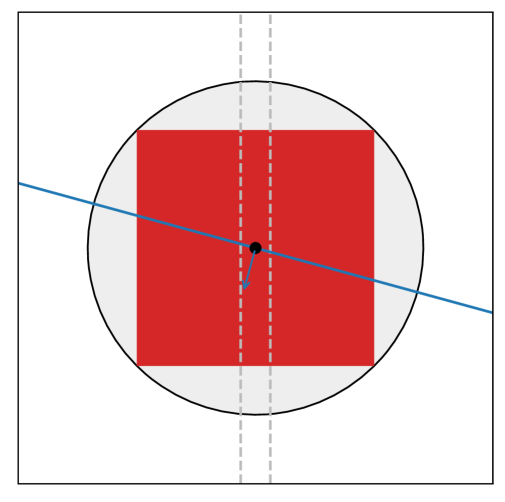
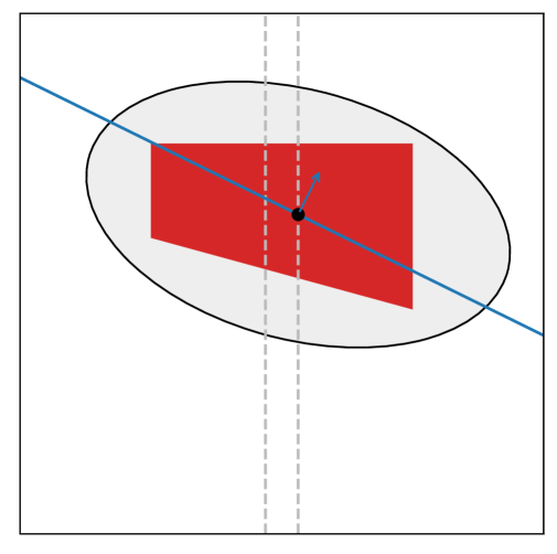
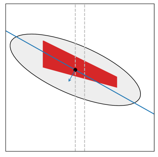
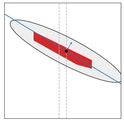
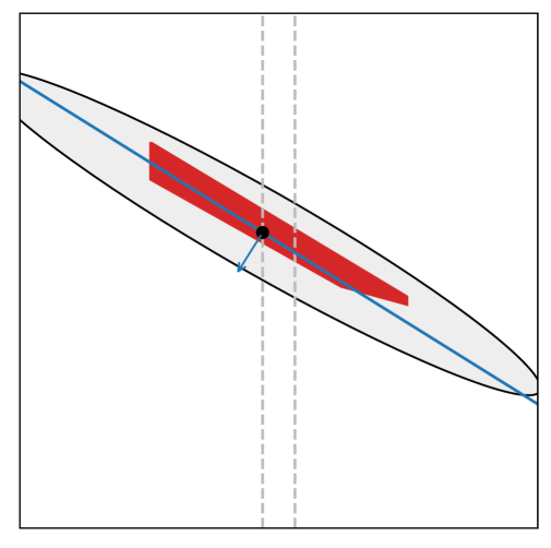
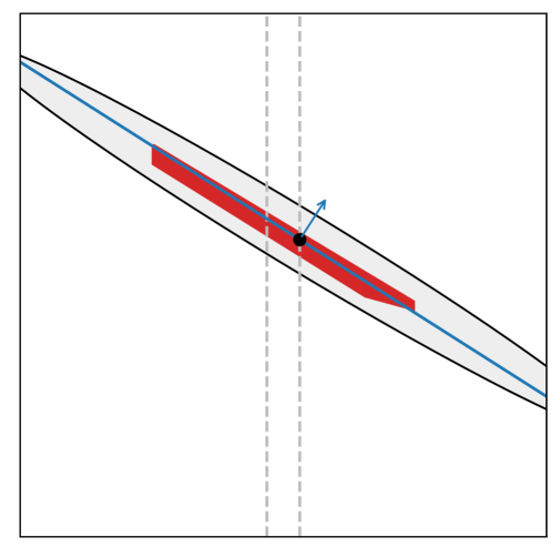
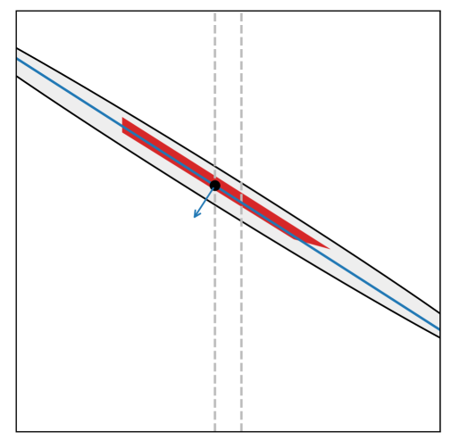
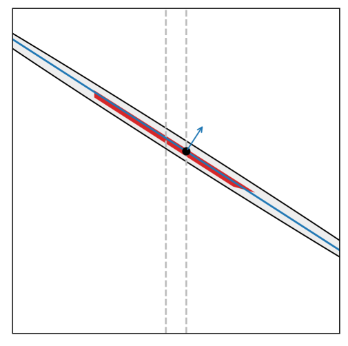
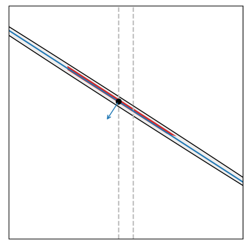
Figure 4: The counterexample for the ellipsoid algorithm without extra-gradient as described in Section 6.3, after $t$ iterations, for $t=0,1,\dots,7,8$. In each plot, the red polygon is the feasible region where Minty points might still lie, and the blue line/arrow indicates the separating direction $F({\bm{a}}^{(t)})$. The two dashed vertical lines correspond to $x=\pm 1/8$.

It is reasonable to ask whether the extra-gradient step in our main algorithm (Algorithm 2) is necessary. In other words, if the extra-gradient step were to be removed, would we still be able to have $\log(1/\epsilon)$ convergence toward an SVI solution under the Minty condition? In this section, we give strong computational evidence that such a guarantee is impossible. We ran the ellipsoid algorithm on polytope ${\mathcal{X}}=[-1,1]^{2}$ and starting ellipse $B_{\sqrt{2}}(\bm{0})$, which is the smallest ellipse containing ${\mathcal{X}}$. At each timestep, given ellipsoid center ${\bm{a}}^{(t)}\in{\mathcal{X}}$, we generated a separating direction $F({\bm{a}}^{(t)})$ such that:

• when $t$ is even, $F({\bm{a}}^{(t)})$ has positive $y$-component, and ${\bm{a}}^{(t+1)}$ has $x$-component $1/8$, and

• when $t$ is odd, $F({\bm{a}}^{(t)})$ has negative $y$-component, and ${\bm{a}}^{(t+1)}$ has $x$-component $-1/8$, and

As shown in Figure 4, the ellipse quickly grows extremely thin along one axis. After $T=1293$ iterations, we observe the following properties.

• The algorithm has not proven that no Minty solution exists. That is, the red polytope in Figure 4 remains nonempty, and in fact the current center ${\bm{a}}^{(T)}$ is a candidate Minty solution.

• The radius of the short axis of the ellipse is less than $1.498\times 10^{-219}$.

• No approximate SVI point has been found: $\norm{F({\bm{a}}^{(t)})}=1$ and $\norm{{\bm{a}}^{(t)}}<0.481$ for every timestep $t$, so the minimum SVI gap of any queried point is at least $0.519$.

• No Lipschitz violation has been found: for every $0\leq s<t\leq T$, we have

  $$\frac{\norm{F({\bm{a}}^{(s)})-F({\bm{a}}^{(t)})}}{\norm{{\bm{a}}^{(s)}-{\bm{a}}^{(t)}}}<7.997.$$

A common idea when using the ellipsoid method for low-dimensional sets is to, once the shortest axis of the ellipse gets small, simply project the problem onto a subspace of smaller dimension and continue. However, this will not work in our setting. Indeed, after such a projection is made, it is possible that $F({\bm{a}}^{(t)})$ has large magnitude in a direction orthogonal to the subspace (so that ${\bm{a}}^{(t)}$ is not an SVI point) and yet $F({\bm{a}}^{(t)})$ gives no separation direction, so ellipsoid cannot proceed.

Thus, even in two dimensions, this counterexample demonstrates that ellipsoid fails to find an approximate SVI solution even when the Minty property holds and the given function is Lipschitz. This demonstrates the need for the additional ideas we introduce in Section 4.2 (namely, the extra-gradient step) beyond the naive ellipsoid method.

7 Conclusion and future research

In summary, we established the first algorithm for computing $\epsilon$-SVI solutions under the Minty condition that has polynomial dependence on both $d$ and $\log(1/\epsilon)$. We also provided several new applications of our main results in optimization and game theory, including the first polynomial-time algorithm for quasar-convex optimization. Our results raise a number of interesting questions for future work. First, one of our main contributions was a technique to tackle the lack of full dimensionality when using the ellipsoid algorithm by using strict separation; it is possible that our approach can be employed to other problems as well. Furthermore, our result concerning strict CCEs only applies to two-player games; while it cannot be generalized to games with more than two players or to tighter equilibrium concepts such as correlated equilibrium [Aumann, 1974], it would still be interesting to characterize classes of games and solution concepts for which such extensions are possible. Finally, our main result provides further motivation for characterizing what problems satisfy the Minty condition and related concepts.

Appendix A Sufficiency of isotropic position

This section shows that assuming ${\mathcal{X}}$ to be in isotropic position is without any loss; we formalize this in the following lemma (cf. Daskalakis et al. [2025, Appendix A]).

Lemma A.1 (Sufficiency of isotropic position).

Let ${\mathcal{X}}\subseteq{\mathcal{B}}_{R}(\bm{0})$ be a convex and compact set, with $R\geq 1$, and $F:{\mathcal{X}}\to\mathbb{R}^{d}$. There is an invertible, affine transformation $\psi$ and a mapping $\tilde{F}:\tilde{{\mathcal{X}}}:=\psi({\mathcal{X}})\to\mathbb{R}^{d}$ such that the following properties hold:

1. $\tilde{{\mathcal{X}}}=\psi({\mathcal{X}})$ is in isotropic position.

2. If $\textsc{VI}({\mathcal{X}},F)$ satisfies the Minty condition, then $\textsc{VI}(\tilde{{\mathcal{X}}},\tilde{F})$ also satisfies the Minty condition.

3. If $\tilde{{\bm{x}}}$ is an $\epsilon$-SVI solution (per Definition B.1) to $\textsc{VI}(\tilde{{\mathcal{X}}},\tilde{F})$, then ${\bm{x}}:=\psi^{-1}(\tilde{{\bm{x}}})$ is a $(2R\epsilon)$-SVI solution to $\textsc{VI}({\mathcal{X}},F)$.

4. If $F$ is $L$-Lipschitz continuous, then $\tilde{F}$ is $(4R^{2}L)$-Lipschitz continuous; if $\|F({\bm{x}})\|\leq B$ for all ${\bm{x}}\in{\mathcal{X}}$, then $\|\tilde{F}(\tilde{{\bm{x}}})\|\leq 2RB$ for all $\tilde{{\bm{x}}}\in\tilde{{\mathcal{X}}}$; and if $F$ satisfies 2.5, then $\tilde{F}$ also satisfies 2.5.

Proof.

Let $\psi({\bm{x}}):=\mathbf{A}{\bm{x}}+\bm{b}$ for an invertible matrix $\mathbf{A}$. Item 1 follows by suitably selecting $\mathbf{A}$ and $\bm{b}$; for example, see the polynomial-time algorithm of Lovász and Vempala [2006].

With regard to Item 2, we proceed as follows. Since $\tilde{{\mathcal{X}}}\supseteq{\mathcal{B}}_{1}(\bm{0})$, there exists ${\bm{x}}\in{\mathcal{B}}_{R}(\bm{0})$ such that $\bm{0}=\mathbf{A}{\bm{x}}+\bm{b}$, implying that $\|\mathbf{A}^{-1}\bm{b}\|\leq R$. Further, for any $\tilde{{\bm{x}}}$ with $\|\tilde{{\bm{x}}}\|=1$, we have $\tilde{{\bm{x}}}=\mathbf{A}{\bm{x}}+\bm{b}$ for some ${\bm{x}}\in{\mathcal{B}}_{R}(\bm{0})$. So, $\|\mathbf{A}^{-1}\tilde{{\bm{x}}}\|=\|\mathbf{A}^{-1}(\tilde{{\bm{x}}}-\bm{b})+\mathbf{A}^{-1}\bm{b}\|\leq\|{\bm{x}}\|+\|\mathbf{A}^{-1}\bm{b}\|\leq 2R$. This implies that $\|\mathbf{A}^{-1}\|\leq 2R$.

Now, we define $\tilde{F}:\tilde{{\mathcal{X}}}\ni\tilde{{\bm{x}}}\mapsto(\mathbf{A}^{-1})^{\top}F(\psi^{-1}(\tilde{{\bm{x}}}))$. Suppose that there is ${\bm{x}}\in{\mathcal{X}}$ such that $\langle F({\bm{x}}^{\prime}),{\bm{x}}^{\prime}-{\bm{x}}\rangle\geq 0$ for all ${\bm{x}}^{\prime}\in{\mathcal{X}}$; that is, $\textsc{VI}({\mathcal{X}},F)$ satisfies the Minty condition. Then, we claim that $\tilde{{\bm{x}}}:=\mathbf{A}{\bm{x}}+\bm{b}$ satisfies the Minty condition with respect to $\textsc{VI}(\tilde{{\mathcal{X}}},\tilde{F})$. Indeed, for any $\tilde{{\bm{x}}}^{\prime}\in\tilde{{\mathcal{X}}}$,

$$\langle\tilde{F}(\tilde{{\bm{x}}}^{\prime}),\tilde{{\bm{x}}}^{\prime}-\tilde{{\bm{x}}}\rangle=\langle(\mathbf{A}^{-1})^{\top}F(\psi^{-1}(\tilde{{\bm{x}}}^{\prime})),\mathbf{A}{\bm{x}}^{\prime}+\bm{b}-\mathbf{A}{\bm{x}}-\bm{b}\rangle=\langle F({\bm{x}}^{\prime}),{\bm{x}}^{\prime}-{\bm{x}}\rangle\geq 0.$$

That is, $\textsc{VI}(\tilde{{\mathcal{X}}},\tilde{F})$ satisfies the Minty condition.

Similarly, for Item 3, suppose $\tilde{{\bm{x}}}\in\tilde{{\mathcal{X}}}^{+\epsilon}$ is an $\epsilon$-SVI solution to $\textsc{VI}(\tilde{{\mathcal{X}}},\tilde{F})$. Then,

$$-\epsilon\leq\langle\tilde{F}(\tilde{{\bm{x}}}),\tilde{{\bm{x}}}^{\prime}-\tilde{{\bm{x}}}\rangle=\langle(\mathbf{A}^{-1})^{\top}F(\psi^{-1}(\tilde{{\bm{x}}})),\mathbf{A}{\bm{x}}^{\prime}+\bm{b}-\mathbf{A}{\bm{x}}-\bm{b}\rangle=\langle F({\bm{x}}),{\bm{x}}^{\prime}-{\bm{x}}\rangle$$

for any ${\mathcal{X}}\ni{\bm{x}}^{\prime}=\psi^{-1}(\tilde{{\bm{x}}}^{\prime})$. Further, letting ${\bm{x}}:=\psi^{-1}(\tilde{{\bm{x}}})$,

$$\left\|{\bm{x}}-\left(\mathbf{A}^{-1}\left(\Pi_{\tilde{{\mathcal{X}}}}(\tilde{{\bm{x}}})-\bm{b}\right)\right)\right\|=\left\|\mathbf{A}^{-1}\left(\tilde{{\bm{x}}}-\Pi_{\tilde{{\mathcal{X}}}}(\tilde{{\bm{x}}})\right)\right\|\leq\|\mathbf{A}^{-1}\|\left\|\tilde{{\bm{x}}}-\Pi_{\tilde{{\mathcal{X}}}}(\tilde{{\bm{x}}})\right\|\leq 2R\epsilon,$$

since $\tilde{{\bm{x}}}\in\tilde{{\mathcal{X}}}^{+\epsilon}$; this implies that ${\bm{x}}\in{\mathcal{X}}^{+(2R\epsilon)}$ because $\mathbf{A}^{-1}(\Pi_{\tilde{{\mathcal{X}}}}(\tilde{{\bm{x}}})-\bm{b})\in{\mathcal{X}}$. We conclude that ${\bm{x}}=\psi^{-1}(\tilde{{\bm{x}}})$ is an $(2R\epsilon)$-SVI solution to $\textsc{VI}({\mathcal{X}},F)$.

We finally deal with Item 4. For any $\tilde{{\bm{x}}},\tilde{{\bm{x}}}^{\prime}\in\tilde{{\mathcal{X}}}$, we have

$$\|\tilde{F}(\tilde{{\bm{x}}})-\tilde{F}(\tilde{{\bm{x}}}^{\prime})\| =\|(\mathbf{A}^{-1})^{\top}(F(\psi^{-1}(\tilde{{\bm{x}}}))-F(\psi^{-1}(\tilde{{\bm{x}}}^{\prime})))\|$$

$$\leq\|\mathbf{A}^{-1}\|\|F(\psi^{-1}(\tilde{{\bm{x}}}))-F(\psi^{-1}(\tilde{{\bm{x}}}^{\prime}))\|$$

$$\leq L\|\mathbf{A}^{-1}\|\|\psi^{-1}(\tilde{{\bm{x}}})-\psi^{-1}(\tilde{{\bm{x}}}^{\prime})\|$$

$$\leq L\|\mathbf{A}^{-1}\|\|\mathbf{A}^{-1}\tilde{{\bm{x}}}-\mathbf{A}^{-1}\tilde{{\bm{x}}}^{\prime}\|$$

$$\leq L\|\mathbf{A}^{-1}\|^{2}\|\tilde{{\bm{x}}}-\tilde{{\bm{x}}}^{\prime}\|\leq 4R^{2}L\|\tilde{{\bm{x}}}-\tilde{{\bm{x}}}^{\prime}\|,$$

where we used the fact that $F$ is $L$-Lipschitz continuous and $\|\mathbf{A}^{-1}\|\leq 2R$.

Next, consider any $\tilde{{\bm{x}}}\in\tilde{{\mathcal{X}}}$. Let ${\bm{x}}=\psi^{-1}(\tilde{{\bm{x}}})=\mathbf{A}^{-1}(\tilde{{\bm{x}}}-\bm{b})$. We have $\|\tilde{F}(\tilde{{\bm{x}}})\|=\|(\mathbf{A}^{-1})^{\top}F({\bm{x}})\|\leq 2RB$, as claimed. The final assertion in Item 4—pertaining to 2.5—is immediate from the definition of $\tilde{F}$. ∎

Appendix B Semi-separation under weak oracles

For completeness, this section explains how our analysis in Section 4.2 can be extended under weak oracles.

We first introduce the relaxation of Definition 1.1 for general convex sets; the only difference is that the solution ${\bm{x}}$ is allowed to belong to ${\mathcal{X}}^{+\epsilon}$, as opposed to ${\mathcal{X}}$ in Definition 1.1. (There is no need to refine Definition 1.2 concerning MVIs since our computational results are about SVIs; even when positing the Minty condition, we do not assume access to an MVI solution.)

Definition B.1 (Relaxation of Definition 1.1 for general convex sets).

Let ${\mathcal{X}}$ be a convex and compact subset of $\mathbb{R}^{d}$ and a mapping $F:{\mathcal{X}}\to\mathbb{R}^{d}$. The $\epsilon$-approximate (Stampacchia) variational inequality (SVI) problem asks for a point ${\bm{x}}\in{\mathcal{X}}^{+\epsilon}$ such that

$$\langle F({\bm{x}}),{\bm{x}}^{\prime}-{\bm{x}}\rangle\geq-\epsilon\quad\forall{\bm{x}}^{\prime}\in{\mathcal{X}}.$$ (28)

We do not insist on satisfying (28) only for ${\bm{x}}^{\prime}\in{\mathcal{X}}^{-\epsilon}$ in light of Remark 2.1. Now, in the context of Section 4.2, it suffices to provide the approximate version of Lemma 4.5.

Lemma B.2.

Suppose that ${\bm{a}}\in{\mathcal{X}}^{+\tilde{\epsilon}}$ is not an $\epsilon$-SVI solution, with $\tilde{\epsilon}<\epsilon$. If $\tilde{{\bm{a}}}\in{\mathcal{X}}^{+\tilde{\epsilon}}$ satisfies

$$\left\langle F({\bm{a}})+\frac{1}{\eta}(\tilde{{\bm{a}}}-{\bm{a}}),{\bm{x}}-\tilde{{\bm{a}}}\right\rangle\geq-B\tilde{\epsilon}\quad\forall{\bm{x}}\in{\mathcal{X}}$$ (29)

with $\eta=1/(2L)$, then

$$\langle F(\tilde{{\bm{a}}}),{\bm{a}}-{\bm{x}}\rangle\geq L\left(B+4LR\right)^{-2}(\epsilon-\tilde{\epsilon})^{2}-\tilde{\epsilon}(3B+6LR).$$ (30)

for any ${\bm{x}}\in{\mathcal{X}}$ that satisfies the Minty VI (2).

In particular, for a sufficiently small $\tilde{\epsilon}\leq\epsilon^{2}\cdot\poly(R^{-1},L^{-1},B^{-1})$, one recovers the same guarantee as in Lemma 4.5 but with a slightly inferior constant.

Proof of Lemma B.2.

We first note that $\tilde{{\bm{a}}}$ can be obtained as an approximation solution to the $\nicefrac{{1}}{{\eta}}$-strongly convex optimization problem

$$\operatorname*{argmin}_{{\bm{x}}\in{\mathcal{X}}}\left\{\langle{\bm{x}},F({\bm{a}})\rangle+\frac{1}{2\eta}\|{\bm{x}}-{\bm{a}}\|^{2}\right\}.$$ (31)

By (29), we have

$$\left\langle F({\bm{a}})+\frac{1}{\eta}(\tilde{{\bm{a}}}-{\bm{a}}),\Pi_{\mathcal{X}}({\bm{a}})-\tilde{{\bm{a}}}\right\rangle\geq-B\tilde{\epsilon}\implies\langle F({\bm{a}}),{\bm{a}}-\tilde{{\bm{a}}}\rangle\geq\frac{1}{\eta}\|{\bm{a}}-\tilde{{\bm{a}}}\|^{2}-\tilde{\epsilon}\left(2B+\frac{2R}{\eta}\right),$$ (32)

where the inequality follows because

$$\left\langle F({\bm{a}})+\frac{1}{\eta}(\tilde{{\bm{a}}}-{\bm{a}}),\Pi_{\mathcal{X}}({\bm{a}})-{\bm{a}}\right\rangle\leq\left\|F({\bm{a}})+\frac{1}{\eta}(\tilde{{\bm{a}}}-{\bm{a}})\right\|\|\Pi_{\mathcal{X}}({\bm{a}})-{\bm{a}}\|\leq\tilde{\epsilon}\left(B+\frac{2R}{\eta}\right).$$

Moreover, for any MVI solution ${\bm{x}}\in{\mathcal{X}}$,

$$\langle F(\tilde{{\bm{a}}}),{\bm{a}}-{\bm{x}}\rangle =\langle F(\tilde{{\bm{a}}}),\tilde{{\bm{a}}}-{\bm{x}}\rangle+\langle F(\tilde{{\bm{a}}}),{\bm{a}}-\tilde{{\bm{a}}}\rangle$$

$$\geq\langle F(\Pi_{\mathcal{X}}(\tilde{{\bm{a}}})),\Pi_{\mathcal{X}}(\tilde{{\bm{a}}})-{\bm{x}}\rangle+\langle F(\tilde{{\bm{a}}}),{\bm{a}}-\tilde{{\bm{a}}}\rangle-\tilde{\epsilon}(B+2LR)$$ (33)

$$\geq\langle F({\bm{a}}),{\bm{a}}-\tilde{{\bm{a}}}\rangle+\langle F(\tilde{{\bm{a}}})-F({\bm{a}}),{\bm{a}}-\tilde{{\bm{a}}}\rangle-\tilde{\epsilon}(B+2LR)$$ (34)

$$\geq\frac{1}{\eta}\|{\bm{a}}-\tilde{{\bm{a}}}\|^{2}-\|F(\tilde{{\bm{a}}})-F({\bm{a}})\|\|{\bm{a}}-\tilde{{\bm{a}}}\|-\tilde{\epsilon}(3B+6LR)$$ (35)

$$\geq\frac{1}{\eta}\|{\bm{a}}-\tilde{{\bm{a}}}\|^{2}-L\|{\bm{a}}-\tilde{{\bm{a}}}\|^{2}-\tilde{\epsilon}(3B+6LR)$$

$$\geq\frac{1}{2\eta}\|{\bm{a}}-\tilde{{\bm{a}}}\|^{2}-\tilde{\epsilon}(3B+6LR),$$ (36)

where (34) uses the fact that ${\bm{x}}$ satisfies (2); (35) follows from (32) and Cauchy-Schwarz; and (36) uses that $F$ is $L$-Lipschitz continuous and $\eta\leq 1/(2L)$. Finally, using again (29), we have that for any ${\bm{x}}\in{\mathcal{X}}$,

$$\left\langle F({\bm{a}})+\frac{1}{\eta}(\tilde{{\bm{a}}}-{\bm{a}}),{\bm{x}}-\tilde{{\bm{a}}}\right\rangle\geq-\tilde{\epsilon}\iff\langle F({\bm{a}}),{\bm{x}}-{\bm{a}}\rangle+\langle F({\bm{a}}),{\bm{a}}-\tilde{{\bm{a}}}\rangle+\frac{1}{\eta}\langle\tilde{{\bm{a}}}-{\bm{a}},{\bm{x}}-\tilde{{\bm{a}}}\rangle\geq-\tilde{\epsilon}.$$ (37)

But ${\bm{a}}\in{\mathcal{X}}^{+\tilde{\epsilon}}$ is not an $\epsilon$-SVI solution, which implies that there exists ${\bm{x}}\in{\mathcal{X}}$ such that $\langle F({\bm{a}}),{\bm{x}}-{\bm{a}}\rangle<-\epsilon$. So, continuing from (37),

$$\epsilon<\langle F({\bm{a}}),{\bm{a}}-\tilde{{\bm{a}}}\rangle+\frac{1}{\eta}\langle\tilde{{\bm{a}}}-{\bm{a}},{\bm{x}}-\tilde{{\bm{a}}}\rangle+\tilde{\epsilon}\leq B\|{\bm{a}}-\tilde{{\bm{a}}}\|+\frac{2R}{\eta}\|{\bm{a}}-\tilde{{\bm{a}}}\|+\tilde{\epsilon},$$

which in turn yields

$$\|{\bm{a}}-\tilde{{\bm{a}}}\|\geq\left(B+4LR\right)^{-1}(\epsilon-\tilde{\epsilon}).$$

Combining with (36), we arrive at (30). ∎

Appendix C Omitted proofs

See 6.4

Proof.

-membership is trivial. For hardness, we reduce from MAX-2-SAT. It is known that there exists an absolute constant $\epsilon$ for which approximating the maximum fraction of satisfiable clauses of a 2-SAT instance to precision better than $\epsilon$ is -complete [Hstad, 2001]. Given a formula $\phi$ with $n$ variables $x_{1},\dots,x_{n}$ and $m$ clauses, let $f:[0,1]^{m}\times[0,1]^{n}\to\mathbb{R}$ be defined by

$$f({\bm{c}},{\bm{x}})=\frac{1}{m}\sum_{j=1}^{m}\quantity(({\bm{c}}_{0}-{\bm{c}}_{j})\ell_{j1}({\bm{x}})+{\bm{c}}_{j}\ell_{j2}({\bm{x}}))$$

where $\ell_{j1}$ and $\ell_{j2}$ are the two literals in clause $j$, that is, each $\ell_{jk}$ has the form either ${\bm{x}}_{i}$ or ${\bm{x}}_{0}-{\bm{x}}_{i}$ for some $i\in[n]$. The values of $f$ are bounded by an absolute constant. In addition, bilinear optimization on $[0,1]^{m}\times[0,1]^{n}$ always admits an integral optimum, so we can restrict our attention to integral values ${\bm{c}}\in\{0,1\}^{m}$ and ${\bm{x}}\in\{0,1\}^{n}$. Now consider some assignment ${\bm{x}}\in\{0,1\}^{n}$, the interpretation that ${\bm{x}}_{i}=1$ if and only if variable $i$ is assigned True. Finally, an optimal ${\bm{c}}\in\{0,1\}^{m}$, for this ${\bm{x}}$, is given by

$${\bm{c}}_{j}=\begin{cases}0&\mbox{\quad if\quad}\text{the first literal of clause $j$ is true in assignment ${\bm{x}}_{1}$}\\ $1$&\mbox{\quad otherwise\quad}\end{cases}$$

Then every clause $j$ contributes $+1/m$ to $f({\bm{c}},{\bm{x}})$ if it is satisfied and $0$ otherwise, so $f({\bm{c}},{\bm{x}})$ is the fraction of clauses satisfied by ${\bm{x}}$. Thus, deciding whether there exist ${\bm{c}},{\bm{x}}$ such that $f({\bm{c}},{\bm{x}})\geq v$ is equivalent to deciding whether a $v$-fraction of clauses can be satisfied. ∎

References

- Abdou et al. [2022] Joseph M. Abdou, Nikolaos Pnevmatikos, Marco Scarsini, and Xavier Venel. Decomposition of games: Some strategic considerations. Mathematics of Operations Research, 47(1):176–208, 2022.
- Adil et al. [2022] Deeksha Adil, Brian Bullins, Arun Jambulapati, and Sushant Sachdeva. Optimal methods for higher-order smooth monotone variational inequalities. arXiv:2205.06167, 2022.
- Aghassi et al. [2006] Michele Aghassi, Dimitris Bertsimas, and Georgia Perakis. Solving asymmetric variational inequalities via convex optimization. Operations Research Letters, 34(5):481–490, 2006.
- Anagnostides et al. [2022a] Ioannis Anagnostides, Gabriele Farina, Ioannis Panageas, and Tuomas Sandholm. Optimistic mirror descent either converges to nash or to strong coarse correlated equilibria in bimatrix games. In Neural Information Processing Systems (NeurIPS), 2022a.
- Anagnostides et al. [2022b] Ioannis Anagnostides, Ioannis Panageas, Gabriele Farina, and Tuomas Sandholm. On last-iterate convergence beyond zero-sum games. In International Conference on Machine Learning (ICML), 2022b.
- Aumann [1974] Robert Aumann. Subjectivity and correlation in randomized strategies. Journal of Mathematical Economics, 1:67–96, 1974.
- Bauschke et al. [2021] Heinz H. Bauschke, Walaa M. Moursi, and Xianfu Wang. Generalized monotone operators and their averaged resolvents. Mathematical Programming, 189(1):55–74, 2021.
- Bensoussan and Lions [2011] Alain Bensoussan and J-L Lions. Applications of variational inequalities in stochastic control, volume 12. Elsevier, 2011.
- Bernasconi et al. [2024] Martino Bernasconi, Matteo Castiglioni, Andrea Celli, and Gabriele Farina. On the role of constraints in the complexity of min-max optimization. arXiv:2411.03248, 2024.
- Boyd and Vandenberghe [2004] Stephen Boyd and Lieven Vandenberghe. Convex Optimization. Cambridge University Press, 2004.
- Bullins and Lai [2022] Brian Bullins and Kevin A Lai. Higher-order methods for convex-concave min-max optimization and monotone variational inequalities. SIAM Journal on Optimization, 32(3):2208–2229, 2022.
- Burachik and Millan [2020] Regina S Burachik and R Diaz Millan. A projection algorithm for non-monotone variational inequalities. Set-Valued and Variational Analysis, 28(1):149–166, 2020.
- Cai et al. [2016] Yang Cai, Ozan Candogan, Constantinos Daskalakis, and Christos H. Papadimitriou. Zero-sum polymatrix games: A generalization of minmax. Mathematics of Operations Research, 41(2):648–655, 2016.
- Cai et al. [2024a] Yang Cai, Constantinos Daskalakis, Haipeng Luo, Chen-Yu Wei, and Weiqiang Zheng. On tractable -equilibria in non-concave games. In Neural Information Processing Systems (NeurIPS), 2024a.
- Cai et al. [2024b] Yang Cai, Argyris Oikonomou, and Weiqiang Zheng. Accelerated algorithms for constrained nonconvex-nonconcave min-max optimization and comonotone inclusion. In International Conference on Machine Learning (ICML), 2024b.
- Candogan et al. [2011] Ozan Candogan, Ishai Menache, Asuman E. Ozdaglar, and Pablo A. Parrilo. Flows and decompositions of games: Harmonic and potential games. Mathematics of Operations Research, 36(3):474–503, 2011.
- Caramanis et al. [2024] Constantine Caramanis, Dimitris Fotakis, Alkis Kalavasis, Vasilis Kontonis, and Christos Tzamos. Optimizing solution-samplers for combinatorial problems: the landscape of policy-gradient methods. In Neural Information Processing Systems (NeurIPS), 2024.
- Combettes and Pennanen [2004] Patrick L. Combettes and Teemu Pennanen. Proximal methods for cohypomonotone operators. SIAM Journal on Control and Optimization, 43(2):731–742, 2004.
- Conitzer [2019] Vincent Conitzer. The exact computational complexity of evolutionarily stable strategies. Mathematics of Operations Research, 44(3):783–792, 2019.
- Cressman et al. [1998] Ross Cressman, William G Morrison, and Jean-François Wen. On the evolutionary dynamics of crime. Canadian Journal of Economics, pages 1101–1117, 1998.
- Danilova et al. [2022] Marina Danilova, Pavel Dvurechensky, Alexander Gasnikov, Eduard Gorbunov, Sergey Guminov, Dmitry Kamzolov, and Innokentiy Shibaev. Recent theoretical advances in non-convex optimization. In High-Dimensional Optimization and Probability: With a View Towards Data Science, pages 79–163. Springer, 2022.
- Daskalakis and Papadimitriou [2011] Constantinos Daskalakis and Christos Papadimitriou. Continuous local search. In ACM-SIAM Symposium on Discrete Algorithms (SODA), 2011.
- Daskalakis et al. [2020] Constantinos Daskalakis, Dylan J. Foster, and Noah Golowich. Independent policy gradient methods for competitive reinforcement learning. In Neural Information Processing Systems (NeurIPS), 2020.
- Daskalakis et al. [2021] Constantinos Daskalakis, Maxwell Fishelson, and Noah Golowich. Near-optimal no-regret learning in general games. In Neural Information Processing Systems (NeurIPS), 2021.
- Daskalakis et al. [2025] Constantinos Daskalakis, Gabriele Farina, Maxwell Fishelson, Charilaos Pipis, and Jon Schneider. Efficient learning and computation of linear correlated equilibrium in general convex games. In Symposium on Theory of Computing (STOC), 2025.
- Davis et al. [2022] Damek Davis, Dmitriy Drusvyatskiy, Yin Tat Lee, Swati Padmanabhan, and Guanghao Ye. A gradient sampling method with complexity guarantees for Lipschitz functions in high and low dimensions. In Neural Information Processing Systems (NeurIPS), 2022.
- Deligkas et al. [2023] Argyrios Deligkas, John Fearnley, Alexandros Hollender, and Themistoklis Melissourgos. Tight inapproximability for graphical games. In AAAI Conference on Artificial Intelligence (AAAI), 2023.