An adaptive multimesh rational approximation scheme for the spectral fractional Laplacian

Abstract.

The paper presents a novel multimesh rational approximation scheme for the numerical solution of the (homogeneous) Dirichlet problem for the spectral fractional Laplacian. The scheme combines a rational approximation of the function $\lambda\mapsto\lambda^{-s}$ with a set of finite element approximations of parameter-dependent non-fractional partial differential equations (PDEs). The key idea that underpins the proposed scheme is that each parametric PDE is numerically solved on an individually tailored finite element mesh. This is in contrast to the existing single-mesh approach, where the same finite element mesh is employed for solving all parametric PDEs. We develop an a posteriori error estimation strategy for the proposed rational approximation scheme and design an adaptive multimesh refinement algorithm. Numerical experiments show improvements in convergence rates compared to the rates for uniform mesh refinement and up to 10 times reduction in computational costs compared to the corresponding adaptive algorithm in the single-mesh setting.

1. Introduction

Fractional partial differential equations (FPDEs) arise in a wide range of applications including anomalous diffusion, porous media, phase separation in fluids, discontinuous deformations (fractures), and spatial statistics (see [19, 25] and the references therein). They have become a powerful mathematical tool in these application areas due to their ability to model nonlocal phenomena and processes that are characterized by interactions at a distance. The development of effective bespoke numerical methods and algorithms for FPDEs is also of significant interest, as the standard computational techniques applied to them generally incur much greater computational costs than if applied to classical (non-fractional) PDE-based models.

In this work, we consider one particular fractional derivative operator, the fractional Laplacian $(-\Delta)^{s}$ ($0<s<1$), that has received the most attention from both the mathematical analysis and numerical analysis communities. Among many non-equivalent definitions of the fractional Laplacian on a bounded domain $\Omega$, our focus here is on the spectral fractional Laplacian (we give precise definition in section 2). For a given $s\in(0,1)$ and $f\in L^{2}(\Omega)$, we consider the following boundary value problem for the spectral fractional Laplacian: find $u:\Omega\to\mathbb{R}$ such that

$$(-\Delta)^{s}u=f\quad\text{in }\Omega,\qquad u=0\quad\text{on }\partial\Omega.$$ (1)

This problem can be discretized directly using, e.g., the finite element method (FEM). However, due to the nonlocal nature of the fractional Laplacian, such a discretization would lead to a dense linear system, see, e.g., [25]. The resulting linear system can become computationally intractable if the number of degrees of freedom is very large, which is often the case when solving 3D problems and/or using a very fine computational mesh. In addition, for small values of $s$, the solution to (1) exhibits boundary layers, calling for approximations that employ adaptive and/or anisotropic mesh refinement, see, e.g., [17, 6].

Several alternative discretization strategies for problems involving the fractional Laplacian (and applicable to more general nonlocal problems) are available in the literature. Among these strategies we mention the methods that employ the Dirichlet-to-Neumann maps to reformulate (1) in 2D as a three-dimensional non-fractional problem (see [26, 5]), reduced basis methods that construct a discrete space of small dimension where the solution $u$ is sought (see [3]), the semi-group method that transforms the elliptic problem (1) into a non-fractional parabolic problem (see [18]), and the methods that employ rational approximations of the function $\lambda\mapsto\lambda^{-s}$ in order to reformulate a fractional PDE as a set of independent non-fractional parameter-dependent PDEs (see [12, 13, 22, 29, 14]). In particular, the strategies combining rational approximations of $\lambda^{-s}$ and finite element discretizations of non-fractional parametric PDEs have become popular. In these strategies, called rational approximation schemes, instead of assembling and solving one dense linear system, the FEM is used to assemble several independent sparse linear systems that can be solved in parallel. The approximate solution to problem (1) is then obtained as a linear combination of those independently generated finite element approximations. The existing rational approximation schemes employ the same finite element space (associated with a single finite element mesh on $\Omega$) for all non-fractional parametric PDE problems; we refer to this approach as a single-mesh scheme.

A posteriori error estimation and adaptive solution techniques are fairly recent topics in the numerical analysis of FPDEs. The following a posteriori error estimation strategies have been developed to guide adaptive mesh refinement in the FEM-based methods for fractional problems: residual-based error estimators [1, 21], a gradient recovery based error estimator [31], and hierarchical error estimators [17, 14].

In this work, we propose a novel multimesh framework for rational approximation schemes where the underlying meshes (and hence FEM approximations) can be different for different non-fractional parametric problems. Within this framework, we develop an a posteriori error estimation strategy that drives adaptive multimesh refinement algorithm for the numerical solution of problem (1). We emphasize that our multimesh construction, the error estimation strategy, and the adaptive algorithm are generic, in the sense that they can be used with any rational approximation of the function $\lambda^{-s}$ (see §3.1 below). Our practical implementation, however, employs a specific rational approximation—the one proposed by Bonito and Pasciak in [12]—but can be easily adapted to other approximations such as, e.g., the BURA-based schemes [22]. Numerical experiments demonstrate two main advantages of our adaptive multimesh framework: faster convergence rates (particularly, for smaller values of $s\in(0,1)$) when compared to the rates for uniform mesh refinement (see [12]), and up to 10 times reduction in computational cost compared to the adaptive algorithm proposed in [14] in the single-mesh setting.

The paper is organized as follows. In section 2, we define the spectral fractional Laplacian operator $(-\Delta)^{s}$ in (1). Section 3 introduces a multimesh rational approximation scheme for problem (1), including the underlying rational approximation of the function $\lambda^{-s}$, finite element discretizations as well as the concept of union mesh that plays a key role in computing the fully discrete solution and in a posteriori error analysis. In section 4, we discuss local hierarchical error indicators and propose two a posteriori estimates of the overall discretization error in the $L^{2}$-norm. An adaptive multimesh refinement algorithm is formulated in section 5. The effectiveness of two error estimation strategies and the performance of the proposed adaptive algorithm are assessed in a series of numerical experiments presented in section 6.

2. The spectral fractional Laplacian

Let $\Omega\subset\mathbb{R}^{d}$ ($d=2,3$) be a connected bounded domain with polygonal/polyhedral boundary $\partial\Omega$ and let $\omega$ be any open connected subset of $\overline{\Omega}$. We denote by $L^{2}(\omega)$ the space of square integrable functions over $\omega$ with the usual inner product $\left(\cdot,\cdot\right)_{2,\omega}$ and the associated norm $\lVert\cdot\rVert_{2,\omega}$. We denote by $H^{1}(\omega)$ the Sobolev space of functions with first-order weak derivatives in $L^{2}(\omega)$; it is endowed with the inner product $\left(\nabla\cdot,\nabla\cdot\right)_{2,\omega}+\left(\cdot,\cdot\right)_{2,\omega}$, and the associated squared norm is given by $\lVert\nabla\cdot\rVert_{2,\omega}^{2}+\lVert\cdot\rVert_{2,\omega}^{2}$. The subspace of functions in $H^{1}(\Omega)$ with zero trace on the boundary $\partial\Omega$ is denoted by $H^{1}_{0}(\Omega)$. The inner product and the norm in $H^{1}_{0}(\Omega)$ are given by $\left(\nabla\cdot,\nabla\cdot\right)_{2,\Omega}$ and $\lVert\nabla\cdot\rVert_{2,\Omega}$, respectively. In what follows, when $\omega=\Omega$, we will omit the dependence on $\omega$ in the subscripts of inner products and norms.

Let ${\color[rgb]{0,0,0}\{(\psi_{i},\lambda_{i});\ i\in\mathbb{N}\}}\subset L^{2}(\Omega)\times\mathbb{R}_{>0}$ be the spectrum of the standard negative Laplacian $-\Delta$ on $\Omega$ with zero Dirichlet boundary condition on $\partial\Omega$. In other words, the eigenvalues $\lambda_{i}\in\mathbb{R}_{>0}$ and the eigenfunctions $\psi_{i}:\Omega\to\mathbb{R}$ are defined by the following eigenvalue problem:

$$-\Delta\psi_{i}=\lambda_{i}\psi_{i}\quad\text{in }\Omega,\quad\psi_{i}=0\quad\text{on }\partial\Omega.$$

We assume that the eigenvalues $\lambda_{i}$ are sorted in increasing order and we denote by $\lambda_{0}\in\mathbb{R}_{>0}$ a lower bound such that

$$\lambda_{0}\leqslant\lambda_{1}\leqslant\ldots\leqslant\lambda_{i}\leqslant\lambda_{i+1}\leqslant\ldots.$$

Furthermore, the set $\{\psi_{i};\ i\in\mathbb{N}\}$ is an orthonormal basis in $L^{2}(\Omega)$.

For any $s\in(0,1)$, let us now consider the spectral fractional Laplacian operator $(-\Delta)^{s}$ with zero Dirichlet boundary condition. This is a pseudo-differential operator that is defined via its action on the eigenfunctions $\psi_{i}$ of the standard Laplacian as follows:

$$(-\Delta)^{s}\psi_{i}=\lambda_{i}^{s}\psi_{i}\quad\forall i\in\mathbb{N}.$$

For any function $v\in{\mathbb{H}}^{s}(\Omega):=\Big{\{}v\in L^{2}(\Omega),\ \sum\limits_{i=1}^{\infty}\lambda_{i}^{s}\left(v,\psi_{i}\right)_{2}^{2}<\infty\Big{\}}$, we have

$$(-\Delta)^{s}v:=\sum_{i=1}^{\infty}\lambda_{i}^{s}\left(v,\psi_{i}\right)_{2}\psi_{i}.$$

Using this representation we conclude that the solution $u$ to problem (1) admits the following expansion:

$$u=\sum_{i=1}^{\infty}\lambda_{i}^{-s}\left(f,\psi_{i}\right)_{2}\psi_{i}.$$ (2)

3. A multimesh rational approximation scheme

In this section, we describe two components of rational approximations schemes: a rational approximation of the function $\lambda\mapsto\lambda^{-s}$ and the finite element discretization. We also introduce the union mesh as a key ingredient of our multimesh construction.

3.1. Rational approximations

The idea of rational approximation schemes in the context of solving problem (1) hinges on approximating the function $\lambda\mapsto\lambda^{-s}$ for $\lambda\in[\lambda_{0},+\infty)$ by rational functions $\lambda\mapsto\mathcal{Q}_{s}^{\kappa}(\lambda)$ of the form

$$\mathcal{Q}_{s}^{\kappa}(\lambda):=C(s,\kappa)\sum_{l=1}^{N(\kappa)}a_{l}(s,\kappa)\big{(}c_{l}(s,\kappa)+b_{l}(s,\kappa)\lambda\big{)}^{-1}.$$ (3)

Here, $\kappa\in\mathbb{R}_{>0}$ encodes the fineness of this approximation, $\mathbb{N}_{>0}\ni N(\kappa)\to+\infty$ as $\kappa\to 0$, and the coefficients $C,\,a_{l},\,b_{l},\,c_{l}\in\mathbb{R}_{>0}$ for all $l=1,\ldots,N(\kappa)$ are chosen so that $\mathcal{Q}_{s}^{\kappa}$ converges exponentially fast to $\lambda^{-s}$ (uniformly on the interval $[\lambda_{0},+\infty)$) as $\kappa\to 0$. In other words, there exists $\varepsilon_{s}(\kappa)\in\mathbb{R}_{>0}$ independent of $\lambda$ such that

$$\left\lvert\lambda^{-s}-\mathcal{Q}_{s}^{\kappa}(\lambda)\right\rvert\leqslant\varepsilon_{s}(\kappa)\quad\forall\lambda\in[\lambda_{0},+\infty),$$ (4)

where $\varepsilon_{s}(\kappa)\to 0$ exponentially fast as $\kappa\to 0$.

The rational approximation $\mathcal{Q}_{s}^{\kappa}$ defined in (3) can be used to derive a semi-discrete approximation of the solution $u$ to problem (1). Specifically, replacing $\lambda_{i}^{-s}$ with $\mathcal{Q}_{s}^{\kappa}(\lambda_{i})$ for all $i\in\mathbb{N}$ in representation (2) of the solution $u$, the following semi-discrete approximation of $u$ is obtained (see, e.g., [12] for full details):

$$u_{\kappa}:=C(s,\kappa)\sum_{l=1}^{N(\kappa)}a_{l}(s,\kappa)w_{l},$$ (5)

where each function $w_{l}:\Omega\to\mathbb{R}$ ($l=1,\ldots,N(\kappa)$) solves the corresponding non-fractional reaction-diffusion problem

$${\color[rgb]{0,0,0}-b_{l}(s,\kappa)\Delta w_{l}+c_{l}(s,\kappa)w_{l}=f\quad\text{in }\Omega,\qquad w_{l}=0\quad\text{on }\partial\Omega.}$$ (6)

The fully discrete approximation of $u$ is then obtained by discretizing each parametric problem (6) (using, e.g., the FEM, see §3.2) and replacing the functions $w_{l}$ in (5) with their (finite element) approximations.

3.1.1. The Bonito–Pasciak rational approximation

For a fixed $s\in(0,1)$, the Bonito–Pasciak (BP) rational approximation scheme for solving problem (1) is based on the following identity that is derived from the Balakrishnan formula in [4]:

$$\lambda^{-s}=\frac{2\sin(\pi s)}{\pi}\int_{-\infty}^{+\infty}\operatorname{e}^{2sy}\left(1+\operatorname{e}^{2y}\lambda\right)^{-1}\ \,\mathrm{d}y.$$ (7)

Hence, for a given fineness parameter $\kappa\in\mathbb{R}_{>0}$, the rational approximation $\mathcal{Q}_{s}^{\kappa}(\lambda)$ of $\lambda^{-s}$ is obtained in [12] by discretizing the integral in (7) via a rectangle quadrature rule:

$$\mathcal{Q}_{s}^{\kappa}(\lambda):=\frac{2\kappa\sin(\pi s)}{\pi}\sum_{j=-M_{-}(\kappa)}^{M_{+}(\kappa)}\operatorname{e}^{2sj\kappa}\left(1+\operatorname{e}^{2j\kappa}\lambda\right)^{-1},$$ (8)

where

$$M_{-}(\kappa):=\left\lceil\frac{\pi^{2}}{4s\kappa^{2}}\right\rceil\quad\text{and}\quad M_{+}(\kappa):=\left\lceil\frac{\pi^{2}}{4(1-s)\kappa^{2}}\right\rceil$$

with $\lceil\cdot\rceil$ denoting the ceiling function.

Setting $l:=j+M_{-}(\kappa)+1$ and $N(\kappa):=M_{+}(\kappa)+M_{-}(\kappa)+1$, the right-hand side of (8) can be written in the generic form given by (3) with

$$C(s,\kappa)=\frac{2\kappa\sin(\pi s)}{\pi},\qquad a_{l}(s,\kappa)=\exp(2s(l-M_{-}(\kappa)-1)\kappa),$$ (9a)

$$b_{l}(s,\kappa)=\exp(2(l-M_{-}(\kappa)-1)\kappa),\qquad c_{l}(s,\kappa)=1.$$ (9b)

This specific choice of $\mathcal{Q}_{s}^{\kappa}$ satisfies the error bound in (4) with

$$\varepsilon_{s}(\kappa):=\frac{2\sin(\pi s)}{\pi}\left[\frac{1}{2s}+\frac{1}{(2-2s)\lambda_{0}}\right]\left[\frac{\operatorname{e}^{-\pi^{2}/(4\kappa)}}{\sinh(\pi^{2}/(4\kappa))}+\operatorname{e}^{-\pi^{2}/(2\kappa)}\right]$$ (10)

which tends to zero exponentially fast as $\kappa\to 0$; see [12, Remark 3.1].

We refer to [9, 10, 11, 13] for applications of the rational approximation given by (8) to the discretization of various types of fractional PDEs.

From now on, to simplify the notation, we will omit the dependence of the summation limit $N$ and the coefficients $C,\,a_{l},\,b_{l},\,c_{l}$ in (3) on $s$ and $\kappa$.

3.2. Finite element discretization

As it was outlined above, in order to obtain a fully discrete approximation of the solution to problem (1) one needs to discretize each parametric problem (6). To that end, similar to [12, 14], we use the FEM. We note that the diffusion and/or reaction coefficients for parametric problems (6) may vary significantly between different problems; for example, in the case of the BP rational approximation (8), the diffusion coefficients $(b_{l})_{l=1}^{N}$ vary from extremely small for $l=1$ to very large for $l=N$ (cf. (9b)). Thus, as discussed in [14, Section 9.1.1], using the same finite element mesh for all parametric problems may lead to wasted computational resources, since some of these problems will be discretized on an over-refined mesh. Therefore, the key idea and the main novelty of this study is to allow different meshes to be used for the finite element discretization of different parametric problems in (6). In particular, we will propose an algorithm that adaptively refines the finite element mesh individually for each parametric problem and employs an overlay of all the meshes (referred to as the union mesh) in order to compute the fully discrete approximation of the solution $u$ to the fractional Laplacian problem (1).

For $m\in\mathbb{N}_{0}$, let $\left\{\mathcal{T}_{l}^{m},\ l=1,\ldots,N\right\}$ be a family of meshes on $\Omega$, where each mesh $\mathcal{T}_{l}^{m}$ is a conforming partition of $\Omega$ into compact non-degenerate simplices (cells). The mesh $\mathcal{T}_{l}^{m}$ is associated with the $l$-th parametric problem in (6), and the subscript $m$ is the iteration counter in our adaptive algorithm, i.e., for each $l=1,\ldots,N$, the mesh $\mathcal{T}^{m+1}_{l}$ is either a refinement of the mesh $\mathcal{T}_{l}^{m}$ or $\mathcal{T}^{m+1}_{l}=\mathcal{T}_{l}^{m}$. For mesh refinement, we employ newest vertex bisection (NVB); see, e.g., [28, 23]. We assume that any mesh $\mathcal{T}_{l}^{m}$ employed for the discretization of parametric problems in (6) can be obtained by applying NVB refinement(s) to a given (coarse) initial mesh $\mathcal{T}^{0}$.

Given a mesh $\mathcal{T}_{l}^{m}$, we denote by $K$ a cell, by $F$ an edge (in two dimensions) or a face (in three dimensions), and by $\chi$ a vertex of $\mathcal{T}_{l}^{m}$. For a cell $K$, the set of edges/faces of $K$ is denoted by $\partial K$. Furthermore, $\mathcal{F}_{l}^{m}$ denotes the set of interior edges/faces of $\mathcal{T}_{l}^{m}$, and for any edge/face $F\in\mathcal{F}_{l}^{m}$, we denote by $n_{F}$ a unit normal vector to $F$. We assume that these normal vectors are fixed once and for all. Let $v$ be a sufficiently regular function. For an edge/face $F\in\mathcal{F}_{l}^{m}$ shared by two cells $K_{1}$ and $K_{2}$, we denote by $\left\llbracket v\right\rrbracket_{F}:=v_{|K_{1}}-v_{|K_{2}}$ the jump of $v$ across $F$, and let $\partial_{n_{F}}v:=\nabla v\cdot n_{F}$ denote the normal derivative of $v$.

Let $\omega\subseteq\Omega$, $p\in\mathbb{N}$ and let $\mathcal{P}^{p}(\omega)$ be the space of polynomial functions of degree $p$ over $\omega$. We denote by $\mathcal{S}^{m,p}_{l}$ the Lagrange finite element space of degree $p$ associated with the mesh $\mathcal{T}_{l}^{m}$:

$$\mathcal{S}^{m,p}_{l}:=\left\{v\in{\color[rgb]{0,0,0}H^{1}_{0}(\Omega)};\ v\in\mathcal{P}^{p}(K)\ \text{for all}\ K\in\mathcal{T}_{l}^{m}\right\}.$$ (11)

For $l=1,\ldots,N$, we introduce the Galerkin finite element formulation of the parametric problem (6): find $w_{l}^{m}\in\mathcal{S}^{m,p}_{l}$ satisfying

$$b_{l}\left(\nabla w_{l}^{m},\nabla v\right)_{2}+c_{l}\left(w_{l}^{m},v\right)_{2}=\left(f,v\right)_{2}\quad\forall v\in\mathcal{S}^{m,p}_{l}.$$ (12)

Thus, $w_{l}^{m}$ is the Galerkin finite element approximation of the solution $w_{l}$ to the parametric problem (6).

3.3. Union mesh

Let us consider a fixed $m\in\mathbb{N}_{0}$ (i.e., a fixed iteration step of the adaptive algorithm that we are going to design). Recall that any two finite element meshes within the family $\left\{\mathcal{T}_{l}^{m};\ l=1,\ldots,N\right\}$ might be different. In practice, in order to combine the corresponding finite element approximations $\left\{w_{l}^{m};\ l=1,\ldots,N\right\}$, we need to introduce a mesh $\widetilde{\mathcal{T}}^{m}$ such that the associated finite element space $\widetilde{\mathcal{S}}^{m,p}:=\big{\{}v\in H^{1}_{0}(\Omega);\ v\in\mathcal{P}^{p}(K)\ \text{for all}\ K\in\widetilde{\mathcal{T}}^{m}\big{\}}$ contains all the functions $w_{l}^{m}$. Since each mesh in the family $\left\{\mathcal{T}_{l}^{m};\ l=1,\ldots,N\right\}$ is either $\mathcal{T}^{0}$ or obtained by NVB refinements of $\mathcal{T}^{0}$, we can define the mesh $\widetilde{\mathcal{T}}^{m}$ as the coarsest common refinement (i.e., the overlay) of all meshes in this family; we will call $\widetilde{\mathcal{T}}^{m}$ the union mesh. Thus, $w_{l}^{m}\in\mathcal{S}^{m,p}_{l}\subset\widetilde{\mathcal{S}}^{m,p}$ for all $l=1,\ldots,N$ and we define the fully discrete approximation of the solution $u$ to problem (1) as follows (cf. (5)):

$$\widetilde{u}_{\kappa}^{m}:=C\sum_{l=1}^{N}a_{l}w_{l}^{m}\,{\color[rgb]{0,0,0}\in\widetilde{\mathcal{S}}^{m,p}}.$$ (13)

4. A posteriori error estimation

The overall discretization error in the $L^{2}(\Omega)$-norm is given by $\lVert u-\widetilde{u}_{\kappa}^{m}\rVert_{2}$, where $u$ is the solution to (1) and $\widetilde{u}_{\kappa}^{m}$ is defined in (13). Using the triangle inequality this error can be bounded as follows

$$\lVert u-\widetilde{u}_{\kappa}^{m}\rVert_{2}\leqslant\lVert u-u_{\kappa}\rVert_{2}+\lVert u_{\kappa}-\widetilde{u}_{\kappa}^{m}\rVert_{2},$$ (14)

where $u_{\kappa}$ is given by (5). On the right-hand side of (14), the contribution $\lVert u-u_{\kappa}\rVert_{2}$ to the overall discretization error can be seen as the rational approximation error, whereas the contribution $\lVert u_{\kappa}-\widetilde{u}_{\kappa}^{m}\rVert_{2}$ can be seen as the finite element discretization error. It turns out that, if $f\in L^{2}(\Omega)$ in (1), the rational approximation error decays with the same rate as $\varepsilon_{s}(\kappa)$ in (4). Indeed, following the proof of [12, Theorem 3.5], it is easy to show that

$$\lVert u-u_{\kappa}\rVert_{2}\leqslant\varepsilon_{s}(\kappa)\lVert f\rVert_{2}.$$ (15)

If the BP rational approximation (8) is employed, then $\varepsilon_{s}(\kappa)$ is given by (10), where the only unknown quantity is the lower bound $\lambda_{0}$ of the Laplacian spectrum. Guaranteed lower bounds of the Laplacian spectrum can be computed, see, e.g., [15, 16]. Therefore, in the case of the BP rational approximation, the right-hand side of (15) is fully computable and provides an upper bound for the rational approximation error $\lVert u-u_{\kappa}\rVert_{2}$. Thus, given a precision tolerance $\mathit{\mathrm{tol}}>0$, we can choose the parameter $\kappa$ in (8) so that

$$\lVert u-u_{\kappa}\rVert_{2}\leqslant\varepsilon_{s}(\kappa)\lVert f\rVert_{2}\ll\mathit{\mathrm{tol}}.$$

In what follows we will assume that the rational approximation is sufficiently accurate so that the corresponding approximation error $\lVert u-u_{\kappa}\rVert_{2}$ is negligible compared to the finite element discretization error and

$$\lVert u-\widetilde{u}_{\kappa}^{m}\rVert_{2}\approx\lVert u_{\kappa}-\widetilde{u}_{\kappa}^{m}\rVert_{2}.$$ (16)

Therefore, in this study, our focus is on the adaptive mesh refinement algorithm driven by a posteriori estimates of the finite element error $\lVert u_{\kappa}-\widetilde{u}_{\kappa}^{m}\rVert_{2}$. We refer to [14, Section 7.2] for details of a refinement algorithm that takes into account both the finite element and the rational approximation errors.

Our adaptive algorithm is steered by hierarchical a posteriori error estimators of the Bank–Weiser type [7]. These estimators are computed using enriched finite element spaces on each cell of the mesh.

4.1. Enriched local finite element spaces

For a cell $K\in\mathcal{T}_{l}^{m}$, we denote by $\mathcal{S}_{l}^{m,p}(K)$ the local Lagrange finite element space of degree $p$ over $K$. The space $\mathcal{S}_{l}^{m,p}(K)$ is in fact the same as $\mathcal{P}^{p}(K)$. Let $\widehat{\mathcal{S}}_{l}^{m}(K)$ denote an enriched local finite element space that is obtained from ${\mathcal{S}}_{l}^{m,p}(K)$ by adding new basis functions. Then, $\widehat{\mathcal{S}}_{l}^{m}(K)$ can be decomposed as

$$\widehat{\mathcal{S}}_{l}^{m}(K)=\mathcal{S}_{l}^{m,p}(K)\oplus\mathcal{V}_{l}^{m}(K),$$ (17)

where ${\mathcal{V}}_{l}^{m}(K)\subset H^{1}(K)$ and ${\mathcal{V}}_{l}^{m}(K)\cap{\mathcal{S}}_{l}^{m,p}(K)=\{0\}$. The subspace ${\mathcal{V}}_{l}^{m}(K)$ in (17) is called the enrichment space. Similarly, for a cell $K$ of the union mesh $\widetilde{\mathcal{T}}^{m}$, we denote the enrichment space by $\widetilde{\mathcal{V}}^{m}(K)$.

While enriched spaces can be constructed in many different ways (see [30]), the most popular enrichment strategies are known as $p$-enrichment and $h$-enrichment. In $p$-enrichment, the space $\widehat{\mathcal{S}}_{l}^{m}(K)$ is defined as the finite element space of a higher polynomial degree $\widehat{p}>p$, i.e., $\widehat{\mathcal{S}}_{l}^{m}(K):=\mathcal{S}_{l}^{m,\widehat{p}}(K).$ In this case, the enrichment space $\mathcal{V}_{l}^{m}(K)$ in (17) is the space of polynomials of degree $\widehat{p}$ defined over $K$ and vanishing at the degrees of freedom of $\mathcal{S}_{l}^{m,p}(K)$. Specific examples of $p$-enrichment can be found in [7].

In $h$-enrichment, the space $\widehat{\mathcal{S}}_{l}^{m}(K)$ is defined as the Lagrange finite element space of degree $p$ associated with a uniform partition of the cell $K$. In this case, the space $\mathcal{V}_{l}^{m}(K)$ is the space of (continuous) piecewise polynomials of degree $p$ defined over a uniform partition of $K$ and vanishing at the degrees of freedom of $\mathcal{S}_{l}^{m,p}(K)$. We refer to [2] for specific examples of $h$-enrichment.

4.2. Local error estimation

Let $K$ be a cell of $\mathcal{T}_{l}^{m}$ for some $l=1,\ldots,N$. In the Bank–Weiser error estimation strategy, the enrichment space ${\mathcal{V}}_{l}^{m}(K)$ in (17) is utilized to obtain a local estimator approximating the finite element error on the cell $K$. More precisely, this error estimator is defined as the solution to a local Neumann problem on $K$. The right-hand side of this problem is written it terms of the interior and edge residuals associated with the Galerkin approximation $w_{l}^{m}$ satisfying (12). The interior and edge residuals are denoted by $r_{l,K}^{m}$ and $J_{l,F}^{m}$, respectively, and defined as follows:

$$r_{l,K}^{m}:=(f-c_{l}w_{l}^{m}+b_{l}\Delta w_{l}^{m})|_{K}$$ (18)

and

$$J_{l,F}^{m}:=\begin{cases}b_{l}\llbracket\partial_{n_{F}}w_{l}^{m}\rrbracket_{F}&\text{if }F\in\mathcal{F}_{l}^{m},\\ 0&\text{otherwise.}\end{cases}$$ (19)

Then, the local Neumann problem associated with $K$ reads as: find $e_{l,K}^{m}\in\mathcal{V}_{l}^{m}(K)$ such that for all $v\in\mathcal{V}_{l}^{m}(K)$ there holds

$$b_{l}\left(\nabla e_{l,K}^{m},\nabla v\right)_{2,K}+c_{l}\left(e_{l,K}^{m},v\right)_{2,K}=\left(r_{l,K}^{m},v\right)_{2,K}-\frac{1}{2}\sum_{F\in\partial K}\left(J_{l,F}^{m},v\right)_{2,F}.$$ (20)

The function $e_{l,K}^{m}$ is an approximation of the local error $(w_{l}-w_{l}^{m})|_{K}$ and, consequently, we consider the following local error indicators:

$$\eta_{l,K}^{m}:=\lVert e_{l,K}^{m}\rVert_{2,K}\approx\lVert w_{l}-w_{l}^{m}\rVert_{2,K}.$$ (21)

For each $l=1,\ldots,N$, the local error estimates $\{\eta_{l,K}^{m};\ K\in\mathcal{T}_{l}^{m}\}$ will be used in our adaptive algorithm to mark the cells of $\mathcal{T}_{l}^{m}$ for refinement.

4.3. Global error estimation

In the previous section we have introduced the local error indicators that will be guiding adaptive refinement of finite element meshes. Our goal now is to obtain a computable estimate of the global finite element error $\lVert u_{\kappa}-\widetilde{u}_{\kappa}^{m}\rVert_{2}$, where $u_{\kappa}$ is given by (5) and $\widetilde{u}_{\kappa}^{m}$ is defined in (13). Global error estimates are used to control the overall (finite element) error across the computational domain and, for a given tolerance, they provide a stopping criterion in adaptive algorithms.

If the same finite element mesh is employed for all parametric problems (12), i.e., if $\mathcal{T}_{l}^{m}=\mathcal{T}^{m}$ for all $l=1,\ldots,N$, then obtaining a global error estimate is straightforward. Indeed, for each cell $K\in\mathcal{T}^{m}=\widetilde{\mathcal{T}}^{m}$, the error estimators $e_{l,K}^{m}$ defined by (20) can be combined across all parametric problems and one can define

$$\widetilde{e}_{K}^{m}:=C\sum_{l=1}^{N}a_{l}e_{l,K}^{m}$$ (22)

as an approximation of the local error $(u_{\kappa}-\widetilde{u}_{\kappa}^{m})|_{K}$; cf. (5), (13). Hence, the global error estimate $\widetilde{\eta}^{m}$ can be easily defined as follows:

$$\lVert u_{\kappa}-\widetilde{u}_{\kappa}^{m}\rVert_{2}^{2}=\sum_{K\in{\mathcal{T}}^{m}}\lVert u_{\kappa}-\widetilde{u}_{\kappa}^{m}\rVert_{2,K}^{2}\approx\sum_{K\in{\mathcal{T}}^{m}}\lVert\widetilde{e}_{K}^{m}\rVert_{2,K}^{2}=:(\widetilde{\eta}^{m})^{2}.$$ (23)

This approach to the error estimation within the single-mesh discretization framework for the spectral fractional Laplacian has been first proposed in [14]. The numerical experiments included in [14] have demonstrated the effectivity of this approach.

In the multimesh discretization framework studied in our work, there is no straightforward way to combine local error estimators $e_{l,K}^{m}$ over parametric problems, simply because the meshes underlying finite element approximations for different parametric problems may not share a particular cell $K$. Notably, the definition of $\widetilde{e}_{K}^{m}$ in (22) is no longer valid in this setting. We propose two approaches to address this issue in deriving a computable global error estimate in the multimesh setting.

4.3.1. Global error estimation based on the triangle inequality

The first approach relies on the triangle inequality to obtain a bound on the true error as follows:

$$\lVert u_{\kappa}-\widetilde{u}_{\kappa}^{m}\rVert_{2}=\left\lVert C\sum_{l=1}^{N}a_{l}w_{l}-C\sum_{l=1}^{N}a_{l}w_{l}^{m}\right\rVert_{2}\leqslant C\sum_{l=1}^{N}a_{l}\lVert w_{l}-w_{l}^{m}\rVert_{2}.$$ (24)

Using the local error estimates in (21), we define the global error estimates $\{\eta_{l}^{m};\ l=1,\ldots,N\}$ independently for each parametric problem as follows:

$$(\eta_{l}^{m})^{2}:=\sum_{K\in\mathcal{T}_{l}^{m}}(\eta_{l,K}^{m})^{2}\quad\forall l=1,\ldots,N.$$ (25)

Thus, from (21) we have

$$\lVert w_{l}-w_{l}^{m}\rVert_{2}\approx\eta_{l}^{m}.$$ (26)

Then the overall global error estimate is defined as

$$\eta^{m}:=C\sum_{l=1}^{N}a_{l}\eta_{l}^{m}\overset{\eqref{eq:global_parametric_estimator}}{=}C\sum_{l=1}^{N}a_{l}\bigg{[}\sum_{K\in\mathcal{T}_{l}^{m}}(\eta_{l,K}^{m})^{2}\bigg{]}^{1/2}$$ (27)

and there holds

$$\lVert u-\widetilde{u}_{\kappa}^{m}\rVert_{2}\overset{\eqref{eq:neglect_rational_error}}{\approx}\lVert u_{\kappa}-\widetilde{u}_{\kappa}^{m}\rVert_{2}\overset{\eqref{eq:bound_error_triangle_inequality}}{\leqslant}C\sum_{l=1}^{N}a_{l}\lVert w_{l}-w_{l}^{m}\rVert_{2}\overset{\eqref{eq:local_error_estimator}}{\approx}C\sum_{l=1}^{N}a_{l}\eta_{l}^{m}=\eta^{m}.$$ (28)

This approach has the advantage of being very easy to implement. While $\eta^{m}$ given by (27) is cheap to compute from the local error indicators $\{\eta_{l,K}^{m};\ K\in\mathcal{T}_{l}^{m},\ l=1,\ldots,N\}$, the use of the triangle inequality in (24) can affect the effectivity of the resulting global error estimate.

4.3.2. Global error estimation based on the union mesh

In our second approach, instead of using the error indicators $\eta_{l,K}^{m}$ from the meshes $\mathcal{T}_{l}^{m}$ ($l=1,\ldots,N$), we compute the local error estimators directly on each cell $\widetilde{K}$ of the union mesh $\widetilde{\mathcal{T}}^{m}$. In this case, the local Neumann problem reads as follows: find $e_{l,\widetilde{K}}^{m}\in\widetilde{\mathcal{V}}^{m}(\widetilde{K})$ such that for all $v\in\widetilde{\mathcal{V}}^{m}(\widetilde{K})$ there holds

$$b_{l}\!\left(\nabla e_{l,\widetilde{K}}^{m},\nabla v\right)_{2,\widetilde{K}}+c_{l}\!\left(e_{l,\widetilde{K}}^{m},v\right)_{2,\widetilde{K}}=\!\left(r_{l,\widetilde{K}}^{m},v\right)_{2,\widetilde{K}}-\frac{1}{2}\sum_{\widetilde{F}\in\partial\widetilde{K}}\!\left(J_{l,\widetilde{F}}^{m},v\right)_{2,\widetilde{F}},$$ (29)

where, for each $l=1,\ldots,N$, the residuals $r_{l,\widetilde{K}}^{m}$ and $J_{l,\widetilde{F}}^{m}$ (for each $\widetilde{F}\in\partial\widetilde{K}$) are computed similarly to (18) and (19) from the parametric solutions $w_{l}^{m}$ interpolated at the degrees of freedom associated with the union mesh $\widetilde{\mathcal{T}}^{m}$. Thus, for each cell $\widetilde{K}$ of the union mesh, we obtain an approximation $e_{l,\widetilde{K}}^{m}\in\widetilde{\mathcal{V}}^{m}(\widetilde{K})$ of the local error $(w_{l}-w_{l}^{m})|_{\widetilde{K}}$. Then, in analogy with (22), we define

$$\widetilde{e}_{\widetilde{K}}^{m}:=C\sum_{l=1}^{N}a_{l}\widetilde{e}_{l,\widetilde{K}}^{m}$$

as an approximation of the local error $(u_{\kappa}-\widetilde{u}_{\kappa}^{m})|_{\widetilde{K}}$ for each $\widetilde{K}\in\widetilde{\mathcal{T}}^{m}$. Then $\lVert u_{\kappa}-\widetilde{u}_{\kappa}^{m}\rVert_{2,\widetilde{K}}\approx\lVert\widetilde{e}_{\widetilde{K}}^{m}\rVert_{2,\widetilde{K}}$ and defining the overall global error estimate as

$$\widetilde{\eta}^{m}:=\Bigg{[}\sum_{\widetilde{K}\in\widetilde{\mathcal{T}}^{m}}\lVert\widetilde{e}_{\widetilde{K}}^{m}\rVert_{2,\widetilde{K}}^{2}\Bigg{]}^{1/2},$$ (30)

there holds (cf. (23) in the single-mesh case)

$$\lVert u-\widetilde{u}_{\kappa}^{m}\rVert_{2}\overset{\eqref{eq:neglect_rational_error}}{\approx}\lVert u_{\kappa}-\widetilde{u}_{\kappa}^{m}\rVert_{2}=\Bigg{[}\sum_{\widetilde{K}\in\widetilde{\mathcal{T}}^{m}}\lVert u_{\kappa}-\widetilde{u}_{\kappa}^{m}\rVert_{2,\widetilde{K}}^{2}\Bigg{]}^{1/2}\approx\widetilde{\eta}^{m}.$$

This approach avoids the triangle inequality in (24) at the expense of being more computationally demanding. It requires the construction of the union mesh $\widetilde{\mathcal{T}}^{m}$, the interpolation of each parametric solution $w_{l}^{m}$ at the degrees of freedom associated with $\widetilde{\mathcal{T}}^{m}$, and the solution of local Neumann problems (29) on the cells of $\widetilde{\mathcal{T}}^{m}$. On the other hand, in the adaptive algorithm, the global error estimate only needs to be computed periodically in order to check whether the stopping criterion is satisfied. Therefore, in order to reduce the overall computational complexity of the algorithm, we compute the global error estimate $\widetilde{\eta}^{m}$ given by (30) and check the stopping criterion only at iterations $m\in\{0,k,2k,3k,\ldots\}$, where $k\in\mathbb{N}$ is fixed.

5. Adaptive multimesh refinement algorithm

The adaptive refinement algorithm generates a sequence of fully discrete approximations $\{\widetilde{u}_{\kappa}^{m};\ m\in\mathbb{N}_{0}\}$ by iterating the following loop:

$$\textbf{Solve}\Longrightarrow\textbf{Estimate}\Longrightarrow\textbf{Mark}\Longrightarrow\textbf{Refine}.$$ (31)

The ingredients of the modules Solve and Estimate were described in §3 and §4, respectively. While these two modules have to be executed for each finite element formulation in (12) on the corresponding underlying mesh, the modules Mark and Refine, discussed below, are designed to optimize the refinement across all the meshes.

5.1. Multimesh marking

The core idea underpinning our marking strategy in the multimesh setting is to consider the local error indicators $\eta_{l,K}^{m}$ (see (21)) from all parametric problems and apply a marking algorithm to the joint set of weighted error indicators $\big{\{}a_{l}\eta_{l,K}^{m};\ K\in\mathcal{T}_{l}^{m},\ l=1,\ldots,N\big{\}}$, where $a_{l}$ are the coefficients in the rational approximation (3) (see also the representations of the semi-discrete and fully discrete approximations in (5) and (13), respectively).

In this study we use Dörfler marking [20], but other marking strategies could also be applied in a similar way. Let $\theta\in(0,1]$ be a fixed marking threshold. For each $l=1,\ldots,N$, the module Mark in the adaptive loop (31) finds a set $\mathcal{M}_{l}^{m}\subseteq\mathcal{T}_{l}^{m}$ such that

$$\theta\,\sum_{l=1}^{N}\sum_{K\in\mathcal{T}_{l}^{m}}\big{(}a_{l}\eta_{l,K}^{m}\big{)}^{2}\leqslant\sum_{l=1}^{N}\sum_{K\in\mathcal{M}_{l}^{m}}\big{(}a_{l}\eta_{l,K}^{m}\big{)}^{2},$$ (32)

with the cumulative cardinality $\sum_{l=1}^{N}\#\mathcal{M}_{l}^{m}$ that is minimized over all the sets that satisfy (32).

5.2. Multimesh refinement

The marking sets $\mathcal{M}^{m}_{l}$ generated by the module Mark are fed into the Refine module that performs local NVB refinement of individual marked cells in each finite element mesh $\mathcal{T}_{l}^{m}$, $l=1,\ldots,N$ (note that some cells which have not been marked but that are adjacent to the marked cells will also need to be bisected in order to ensure the conformity of the resulting refined mesh).

We emphasize here that coefficients $a_{l}$ (see, e.g., (9a)) play an important role in the proposed marking and refinement strategy. Used as weights in Dörfler marking (see (32)), they amplify or diminish contributions of the local error indicators associated with the mesh $\mathcal{T}_{l}^{m}$ according to the significance of the corresponding $l$-th term in the rational approximation (3) and in representation (13). For example, if a coefficient $a_{l}$ is very small, then the $a_{l}$-weighted contributions of the error indicators $\eta_{l,K}^{m}$ ($K\in\mathcal{T}_{l}^{m}$) in (32) will be insignificant, and it is very likely that the corresponding marking set $\mathcal{M}_{l}^{m}$ will be empty. This means that no cell from the mesh $\mathcal{T}_{l}^{m}$ will be selected for refinement. Hence, this mesh $\mathcal{T}_{l}^{m}$ as well as the corresponding finite element approximation and the associated local error indicators will all carry over to the next iteration of the adaptive loop, i.e., $\mathcal{T}_{l}^{m+1}:=\mathcal{T}_{l}^{m}$, $w_{l}^{m+1}:=w_{l}^{m}$, and $\eta_{l,K}^{m+1}:=\eta_{l,K}^{m}$ for all $K\in\mathcal{T}_{l}^{m+1}=\mathcal{T}_{l}^{m}$. Therefore, one will not need to run the solve or error estimation routines for the $l$-th parametric problem during the $(m+1)$-st iteration. Thus, even though rational approximation schemes involve solving many parametric problems (12), employing the multimesh framework allows to develop an adaptive algorithm where only a small number of these problems are actually solved at each iteration of the adaptive loop (except the very first iteration, where all parametric problems have to be solved on the coarsest mesh). We will illustrate this aspect of the multimesh approach when we present numerical results in §6.

5.3. Adaptive algorithm

In this section, we present a generic adaptive algorithm for computing multimesh rational approximations of the solution to problem (1).

The algorithm takes as inputs the fractional power $s\in(0,1)$, an initial (coarse) mesh $\mathcal{T}^{0}$, the Dörfler marking parameter $\theta\in(0,1]$, the stopping tolerance $\mathit{\mathrm{tol}}$, and the counter $k\in\mathbb{N}$ that determines the iterations at which the stopping criterion is checked (these are iterations $0,k,2k,3k,\ldots$). For some $m_{*}\in\mathbb{N}_{0}$, the algorithm generates a sequence $\big{\{}\widetilde{u}_{\kappa}^{m};\ m=0,\ldots,m_{*}\big{\}}$ of fully discrete approximations (computed from parametric Galerkin approximations $w_{l}^{m}\in\mathcal{S}^{m,p}_{l}$ using (13)) and two sequences of global a posteriori error estimates, $\big{\{}\eta^{m};\ m=0,\ldots,m_{*}\big{\}}$ and $\big{\{}\widetilde{\eta}^{m};\ m=0,\ldots,m_{*}\big{\}}$, where $\eta^{m}$ and $\widetilde{\eta}^{m}$ are defined by (27) and (30), respectively.

The adaptive algorithm is listed in Algorithm˜1. It contains the following eight subroutines:

• GenerateRationalScheme($s,\mathit{\mathrm{tol}}$)—a subroutine that computes the coefficients $C$, $a_{l}$, $b_{l}$, $c_{l}$ ($l=1,\ldots,N$) of the rational approximation $\mathcal{Q}^{\kappa}_{s}$ in (3) for a given fractional power $s$ of the Laplacian and a prescribed tolerance $\mathit{\mathrm{tol}}$. As discussed in §4, the parameter $\kappa$ in the rational approximation (3) is chosen such that the error bound $\varepsilon_{s}(\kappa)$ in (4) is negligible compared to $\mathit{\mathrm{tol}}$.

• Solve($\mathcal{T}^{m}_{l},b_{l},c_{l}$)—a subroutine that generates the Galerkin approximation $w_{l}^{m}\in\mathcal{S}^{m,p}_{l}$ satisfying (12).

• Estimate($w^{m}_{l},\mathcal{T}^{m}_{l},b_{l},c_{l}$)—a subroutine that computes local error indicators $\eta_{l,K}^{m}$ ($K\in\mathcal{T}^{m}_{l}$) in (21) by solving the local Neumann problem (20); see the discussion in §4.2.

• Mark($\{\mathcal{T}_{l}^{m},\{\eta_{l,K}^{m}\}_{K\in\mathcal{T}_{l}^{m}},a_{l}\}_{l=1}^{N},\theta$)—a subroutine that generates the marking sets $\mathcal{M}_{l}^{m}$ for all finite element meshes $\mathcal{T}_{l}^{m}$, $l=1,\ldots,N$. The sets $\mathcal{M}_{l}^{m}$ are generated using the Dörfler marking strategy adapted to the multimesh framework; see (32).

• Refine($\mathcal{T}_{l}^{m},\mathcal{M}^{m}_{l}$)—a subroutine that generates a refined mesh $\mathcal{T}_{l}^{m+1}$ as described in §5.2.

• GenerateUnionMesh($\{\mathcal{T}^{m}_{l}\}_{l=1}^{N}$)—a subroutine that generates the union mesh $\widetilde{\mathcal{T}}^{m}$; see §3.3.

• GlobalEstimate($C,\,\{w_{l}^{m},\{\eta_{l,K}^{m}\}_{K\in\mathcal{T}_{l}^{m}},a_{l},b_{l},c_{l}\}_{l=1}^{N},\,\widetilde{\mathcal{T}}^{m}$)—a subroutine that computes two global error estimates $\eta^{m}$ and $\widetilde{\eta}^{m}$ defined in (27) and (30), respectively; see §4.3 for a detailed discussion. In the algorithm, the error estimate $\widetilde{\eta}^{m}$ is used in the stopping criterion on line 13.

• SolutionOnUnionMesh($C,\{w^{m}_{l},a_{l}\}_{l=1}^{N},\widetilde{\mathcal{T}}^{m}$)—a subroutine that computes the fully discrete approximation $\widetilde{u}_{\kappa}^{m}$ from the Galerkin approximations $\{w^{m}_{l}\}_{l=1}^{N}$ interpolated at the nodes (and, if $p>1$, at other degrees of freedom) on the union mesh $\widetilde{\mathcal{T}}^{m}$; see (13).

Algorithm 1 Multimesh finite element discretization and adaptive refinement

1:$s\in(0,1)$, $\mathcal{T}^{0}$, $\theta\in(0,1]$, $\mathit{\mathrm{tol}}>0$, $k\in\mathbb{N}$

2:$\big{\{}C,\ \{a_{l},b_{l},c_{l}\}_{l=1}^{N}\big{\}}\leftarrow$ GenerateRationalScheme($s,\mathit{\mathrm{tol}}$)

3:$\mathcal{T}^{0}_{l}\leftarrow\mathcal{T}^{0}\ \forall l=1,\ldots,N$

4:for $m=0,1,\ldots$ do

5:  for $l=1,\ldots,N$ do

6:   if $m=0$ or ($m\geq 1$ and $\mathcal{T}^{m-1}_{l}\neq\mathcal{T}^{m}_{l}$) then

7:     $w^{m}_{l}$ $\leftarrow$ Solve($\mathcal{T}^{m}_{l},b_{l},c_{l}$)

8:     $\{\eta_{l,K}^{m}\}_{K\in\mathcal{T}^{m}_{l}}$ $\leftarrow$ Estimate($w^{m}_{l},\mathcal{T}^{m}_{l},b_{l},c_{l}$)

9:   end if

10:  end for

11:  if $m\!\mod k=0$ then

12:   $\widetilde{\mathcal{T}}^{m}$ $\leftarrow$ GenerateUnionMesh($\{\mathcal{T}^{m}_{l}\}_{l=1}^{N}$)

13:   $\eta^{m}$, $\widetilde{\eta}^{m}$ $\leftarrow$ GlobalEstimate($C,\{w_{l}^{m},\{\eta_{l,K}^{m}\}_{K\in\mathcal{T}_{l}^{m}},a_{l},b_{l},c_{l}\}_{l=1}^{N},\widetilde{\mathcal{T}}^{m}$)

14:   if $\widetilde{\eta}^{m}<\mathit{\mathrm{tol}}$ then

15:     $\widetilde{u}_{\kappa}^{m}$ $\leftarrow$ SolutionOnUnionMesh($C,\{w^{m}_{l},a_{l}\}_{l=1}^{N},\widetilde{\mathcal{T}}^{m}$)

16:     break

17:   end if

18:  end if

19:  $\{\mathcal{M}^{m}_{l}\}_{l=1}^{N}$ $\leftarrow$ Mark($\{\mathcal{T}_{l}^{m},\{\eta_{l,K}^{m}\}_{K\in\mathcal{T}_{l}^{m}},a_{l}\}_{l=1}^{N},\theta$)

20:  for $l=1,\ldots,N$ do

21:   if $\mathcal{M}^{m}_{l}=\varnothing$ then

22:     $\mathcal{T}^{m+1}_{l}\leftarrow\mathcal{T}^{m}_{l}$

23:     $w^{m+1}_{l}\leftarrow w_{l}^{m}$

24:     for $K\in\mathcal{T}^{m+1}_{l}$ do

25:      $\eta^{m+1}_{l,K}\leftarrow\eta_{l,K}^{m}$

26:     end for

27:   else

28:     $\mathcal{T}^{m+1}_{l}$ $\leftarrow$ Refine($\mathcal{T}_{l}^{m},\mathcal{M}^{m}_{l}$)

29:   end if

30:  end for

31:end for

32:$\big{\{}\widetilde{u}_{\kappa}^{m},\,\eta^{m},\,\widetilde{\eta}^{m}\big{\}}_{m=0}^{m_{*}}$ for some $m_{*}=jk$ with $j\in\mathbb{N}_{0}$

We recall from the discussion in §5.2 that not all finite element meshes will be refined at each iteration of the adaptive algorithm. Indeed, if for a given $l\in\{1,\ldots,N\}$, the marking set $\mathcal{M}^{m}_{l}$ is empty, then the mesh $\mathcal{T}^{m}_{l}$ is not refined at this iteration (i.e., $\mathcal{T}_{l}^{m+1}:=\mathcal{T}_{l}^{m}$), and all the quantities associated with $\mathcal{T}^{m}_{l}$ are carried over to the next iteration (see lines 20–25 in Algorithm 1) saving significant computational resources and reducing the computational time.

Since the parametric problems are independent from each other, we emphasize that the for-loops in $l$ (see lines 4–9 and 19–29 in Algorithm 1) can be parallelized, meaning that each of the subroutines Solve, Estimate, and Refine is run simultaneously for all parametric problems. In addition, given any pair of cells $K$ and $K^{\prime}$ in $\mathcal{T}_{l}^{m}$, the corresponding local problems (20) for $K$ and $K^{\prime}$ are also independent from each other. Therefore, the computation of local a posteriori error indicators in the subroutine Estimate can be vectorized over cells, further reducing the computational time.

6. Numerical results

The aim of this section is threefold. Firstly, we will investigate the effectivity and robustness of two strategies for global error estimation in the multimesh setting (see §4.3). Secondly, we will demonstrate the performance of the adaptive algorithm presented in §5.3. Finally, we will compare the performance of adaptive algorithms (in terms of convergence rates and computational costs) in the single-mesh and multimesh settings. To that end, we will consider three representative test problems for the spectral fractional Laplacian in two dimensions.

The numerical results presented here were produced using a MATLAB implementation of Algorithm 1 within the finite element toolbox T-IFISS [8, 27]. The following implementation details are worth noting:

• in the subroutine GenerateRationalScheme, the Bonito–Pasciak rational approximation (see (8)–(10)) is used; in all computations, we set $\kappa=0.26$ in (8) so that the error bound $\varepsilon_{s}(\kappa)$ in (10) does not exceed $2\cdot 10^{-8}$ for all test cases; this guarantees that the rational approximation error in (15) is significantly smaller than the finite element discretization error and (16) holds;

• the first-order (P1) finite element approximations are employed (i.e., $p=1$ in (11));

• the implementation of the a posteriori error estimation strategy in §4 employs the enrichment space $\mathcal{V}_{l}^{m}(K)$ in (17) that is obtained via $h$-enrichment; more precisely, $\mathcal{V}_{l}^{m}(K)$ contains piecewise linear functions over subelements obtained by uniform (NVB) refinement of $K$ (see, e.g., [2, Figure 5.2] and [8, Section 2.1]);

• local mesh refinement is performed using a variant of the newest vertex bisection method called the longest edge bisection; see [8, Section 2.1] and the references therein for details.

In all numerical experiments presented below, we set the marking threshold (see (32)) to $\theta=0.5$ and set $k=1$ (i.e., the stopping criterion for the global error estimate $\widetilde{\eta}^{m}$ is checked at every iteration of the adaptive loop).

6.1. Test case I: square domain, unit right-hand side function

Let us set $f\equiv 1$ and consider the model problem (1) on the square domain $\Omega=(-1,1)^{2}$. The primary aim of this test case is to investigate the effectivity and robustness of two global error estimation strategies introduced in §4.3 in the multimesh setting. To that end, for $s\in\{0.3,\,0.5,\,0.7\}$, we set $\mathcal{T}^{0}$ as a uniform mesh of 512 right-angled triangles and run our adaptive multimesh refinement algorithm. In addition, for each $s$ from the same range, we generate a reference (fully discrete) solution $u_{\text{ref}}\in{\mathcal{S}}^{\text{ref}}\subset H^{1}_{0}(\Omega)$ to problem (1) using a single, highly refined Shishkin-type mesh $\mathcal{T}^{\text{ref}}$. Such meshes contain anisotropic elements in the boundary layer, they are commonly used for the numerical solution of singularly perturbed differential equations and provide accurate approximations (see, e.g., [24] and the references therein). We use the reference solutions to compute the effectivity indices for global a posteriori error estimates $\eta^{m}$ and $\widetilde{\eta}^{m}$ defined by (27) and (30), respectively. The effectivity indices are defined as follows:

$$\Theta^{m}:=\frac{\eta^{m}}{\lVert u_{\text{ref}}-\widetilde{u}_{\kappa}^{m}\rVert_{2}},\quad\widetilde{\Theta}^{m}:=\frac{\widetilde{\eta}^{m}}{\lVert u_{\text{ref}}-\widetilde{u}_{\kappa}^{m}\rVert_{2}},$$ (33)

where $\widetilde{u}_{\kappa}^{m}$ is the fully discrete approximation generated at iteration $m$ of Algorithm 1.

In Figure 1, for each $s\in\{0.3,\,0.5,\,0.7\}$, we visualize the evolution of global error estimates $\eta^{m}$, $\widetilde{\eta}^{m}$ and the corresponding effectivity indices $\Theta^{m}$, $\widetilde{\Theta}^{m}$. Table 1 gives a more quantitative representation of these results; here, we report the number of degrees of freedom in the final approximation $\widetilde{u}_{\kappa}^{m_{*}}\in\widetilde{\mathcal{S}}^{m_{*},1}$ generated by Algorithm 1 and the associated error estimates $\eta^{m_{*}}$, $\widetilde{\eta}^{m_{*}}$, the number of degrees of freedom in the reference solution $u_{\text{ref}}\in{\mathcal{S}}^{\text{ref}}$ and the corresponding global error estimate $\widetilde{\eta}^{\text{ref}}$ computed using (30), as well as the decay rates (with respect to the total number of degrees of freedom) for $\eta^{m}$ and $\widetilde{\eta}^{m}$. The decay rates in this and other test cases are calculated from a linear regression fit on the corresponding values of error estimates for the last 15 iterations of the adaptive loop, in order to avoid any pre-asymptotic regime to affect the results. We also include in Table 1 the theoretical convergence rates for uniformly refined meshes as predicted by [12, Theorem 4.3].

We note that the dimension of the reference finite element space ${\mathcal{S}}^{\text{ref}}$ is at least 32 times bigger than the number of degrees of freedom in the final approximation $\widetilde{u}_{\kappa}^{m_{*}}$ generated by the adaptive algorithm (see Table 1). As a result, the error estimate $\widetilde{\eta}^{\text{ref}}$ for the reference solution $u_{\text{ref}}$ is an order of magnitude smaller than the error estimate $\widetilde{\eta}^{m}$. This justifies the use of $u_{\text{ref}}$ as a proxy for the true solution to problem (1) when calculating the effectivity indices in (33). The plots in Figure 1 show that the global error estimation strategy based on the union mesh provides a more effective and robust way to estimate the error in multimesh approximations than the strategy based on the triangle inequality. Indeed, the effectivity indices $\widetilde{\Theta}^{m}$ (for the union mesh-based strategy) are only slightly less than unity (which is typical for hierarchical error estimates) and, more importantly, vary insignificantly across iterations, whereas the effectivity indices $\Theta^{m}$ (for the triangle inequality-based strategy) exhibit a mild growth as iterations progress. This results in deterioration of the convergence rate for the error estimates $\eta^{m}$ compared to that of the error estimates $\widetilde{\eta}^{m}$. The convergence rates for the error estimates $\widetilde{\eta}^{m}$ are suboptimal (i.e., less than 1) and they improve as the fractional power $s$ gets closer to 1. These rates are higher than those predicted by [12, Theorem 4.3] for uniformly refined meshes, particularly for smaller $s$.

1

Figure 1. Test case I (multimesh setting; $s\in\{0.3,\,0.5,\,0.7\}$): evolution of global error estimates $\eta^{m}$, $\widetilde{\eta}^{m}$ and the corresponding effectivity indices $\Theta^{m}$, $\widetilde{\Theta}^{m}$.

$s$	0.3	0.5	0.7
$\text{dim}\big{(}\widetilde{\mathcal{S}}^{m_{*},1}\big{)}$	9,485	13,365	34,781
$\eta^{m_{*}}$	3.4e-03	8.2e-04	1.4e-04
$\widetilde{\eta}^{m_{*}}$	1.8e-03	3.8e-04	6.1e-05
$\text{dim}\big{(}{\mathcal{S}}^{\text{ref}}\big{)}$	1,052,507	1,046,529	1,132,624
$\widetilde{\eta}^{\text{ref}}$	1.7e-04	3.1e-05	6.0e-06
decay rate for $\eta^{m}$	0.70	0.81	0.90
decay rate for $\widetilde{\eta}^{m}$	0.82	0.90	0.96
decay rate for uniform refinement	0.55	0.75	0.95

Table 1. Test case I (multilevel setting; $s\in\{0.3,\,0.5,\,0.7\}$): the number of degrees of freedom and the error estimates for the final approximation $\widetilde{u}_{\kappa}^{m_{*}}\,{\in}\,\widetilde{\mathcal{S}}^{m_{*},1}$ generated by Algorithm 1 and for the reference solution $u_{\text{ref}}\,{\in}\,{\mathcal{S}}^{\text{ref}}$, as well as the decay rates for two global error estimates $\eta^{m}$, $\widetilde{\eta}^{m}$ and the theoretical convergence rates for uniform mesh refinement (see [12, Theorem 4.3]).

6.2. Test case II: discontinuous right-hand side function

In this test case, we set $\Omega=(0,1)^{2}$ and solve the model problem (1) with discontinuous right-hand side function defined as

$$f(x,y)=\begin{cases}-1&\text{if }(x,y)\in Q_{1}\cup Q_{2},\\ 1&\text{otherwise},\end{cases}$$

where $Q_{1}$ and $Q_{2}$ are the subsets of $\Omega$ bounded by two quarter-circles of radius 0.6 centered at $(0,0)$ and $(1,1)$, respectively. The discontinuity of $f$ leads to sharp gradients in the solution $u$ along the interfaces, in addition to $u$ exhibiting boundary layers. Furthermore, the presence of curved interfaces in the definition of $f$ makes the use of a priori constructed graded meshes less straightforward than, e.g., in test case I; this further motivates the application of an adaptive mesh refinement algorithm.

For this test case with $s\in\{0.1,\,0.3,\,0.5,\,0.7,\,0.9\}$, we run our adaptive multimesh refinement algorithm (Algorithm 1) as well as its single-mesh version developed in [14]. In each run, we start with the initial uniform mesh $\mathcal{T}^{0}$ of 512 right-angled triangles (see Figure 5). For each $s$, the number $N=N(\kappa)$ of parametric problems as well as the stopping tolerance $\mathit{\mathrm{tol}}$ are shown in Table 2.

In Figure 2, for $s\in\{0.3,\,0.5,\,0.7\}$, we report the evolution of three global a posteriori error estimates: $\widetilde{\eta}^{m}$ defined by (23) in the single-mesh setting as well as $\eta^{m}$ and $\widetilde{\eta}^{m}$ defined, respectively, by (27) and (30) for multimesh discretizations. The decay rates for these three global error estimates as well as the theoretical convergence rates predicted in [12, Theorem 4.3] for uniform mesh refinement are shown in Table 2 for $s\in\{0.1,\,0.3,\,0.5,\,0.7,\,0.9\}$.

We make the following conclusions by looking at Figure 2 and Table 2. Firstly, in the multimesh setting, similarly to test case I, we observe a slower decay of error estimates $\eta^{m}$ compared to that of $\widetilde{\eta}^{m}$. This is again due to the triangle inequality affecting the quality of the error estimation in (28). Secondly, while convergence rates for adaptive algorithms (in both the single-mesh and multimesh settings) are suboptimal for $s\in\{0.1,\,0.3,\,0.5,\,0.7\}$ as expected, these rates exceed the theoretically predicted and experimentally observed rates for uniformly refined meshes (in the single-mesh setting), particularly for smaller values of $s$ (cf. [12]). This demonstrates the advantage of adaptive mesh refinement algorithms in mitigating the singular behavior of the solution $u$ along the discontinuity interfaces in $f$. Again, this advantage is more pronounced for smaller values of $s$. Finally, we only see a marginal improvement of convergence rates in the multimesh setting compared to adaptive single-mesh discretizations, and this improvement diminishes as $s$ increases. For $s=0.9$, both adaptive single-mesh and multimesh discretizations converge with essentially an optimal rate $\mathcal{O}\big{(}\mathrm{dof}^{-1}\big{)}$—the predicted convergence rate for uniformly refined (single-mesh) approximations for this value of $s$.

Figure 2. Test case II: evolution of global error estimates in the single-mesh setting ($\widetilde{\eta}^{m}$ defined by (23)) and in the multimesh setting ($\eta^{m}$ and $\widetilde{\eta}^{m}$ defined by (27) and (30), respectively) for $s\in\{0.3,\,0.5,\,0.7\}$.

$s$	0.1	0.3	0.5	0.7	0.9
$N$	408	176	149	176	408
$\mathit{\mathrm{tol}}$	1e-03	1e-04	2e-05	5e-06	1e-06
$m_{*}$ (adaptive single-mesh)	33	32	29	30	32
$m_{*}$ (adaptive multimesh)	35	30	28	28	30
decay rate for $\widetilde{\eta}^{m}$ (adaptive single-mesh)	0.66	0.86	0.93	0.97	0.99
decay rate for $\eta^{m}$ (adaptive multimesh)	0.64	0.82	0.90	0.93	0.96
decay rate for $\widetilde{\eta}^{m}$ (adaptive multimesh)	0.67	0.89	0.96	0.98	0.99
decay rate for uniform refinement	0.35	0.55	0.75	0.95	1.00

Table 2. Test case II: the number $N$ of parametric problems, the stopping tolerance $\mathit{\mathrm{tol}}$, the number $m_{*}$ of iterations as well as the decay rates for global error estimates in the single-mesh and multimesh settings, and the theoretical convergence rates for uniform refinement in the single-mesh setting (see [12, Theorem 4.3]).

Let us now compare the computational costs of running the adaptive algorithm in the single-mesh and multimesh settings. For $l\in\{1,\ldots,N\}$, we define $\mathrm{cost}_{l}^{m}$ as the number of degrees of freedom in the finite element formulation (12) of the corresponding parametric problem (in other words, $\mathrm{cost}_{l}^{m}=\mathrm{dim}\big{(}\mathcal{S}^{m,1}_{l}\big{)}$). Then, the overall computational cost at iteration $m\in\mathbb{N}_{0}$ of the adaptive algorithm is the sum of $\mathrm{cost}_{l}^{m}$ across all the parametric problems that are actually solved at this iteration (for $m\in\mathbb{N}$, this excludes those parametric problems for which the underlying meshes have not been refined at iteration $m-1$). Thus, recalling that the meshes for all parametric problems are initialized by the coarse mesh $\mathcal{T}^{0}$, the total computational cost at iteration $m\in\mathbb{N}_{0}$ is given by

$$\mathit{\mathrm{totcost}}^{m}:=\begin{cases}\displaystyle N\times\mathrm{cost}_{1}^{0}&\text{if }m=0,\\ \displaystyle\sum_{l\in\mathcal{L}}\mathrm{cost}_{l}^{m}&\text{otherwise},\end{cases}$$ (34)

where $\mathcal{L}\subseteq\{1,\ldots,N\}$ determines the subset of parametric problems for which the underlying meshes have been refined at iteration $m-1$. Note that in the single-mesh setting formula (34) simplifies to

$$\mathit{\mathrm{totcost}}^{m}=N\times\mathrm{cost}_{1}^{m},\quad m\in\mathbb{N}_{0}.$$

The cumulative cost at the $m$-th iteration of the adaptive algorithm is defined as follows:

$$\mathrm{cumcost}^{m}:=\sum_{j=1}^{m}\mathit{\mathrm{totcost}}^{j}.$$ (35)

Figure 3 shows the growth of cumulative costs for computing adaptively refined approximations. Here, we plot the cumulative costs against global a posteriori error estimates $\widetilde{\eta}^{m}$ in the single-mesh and multimesh settings (see (23) and (30), respectively). The plots show that computing an adaptive multimesh approximation can be up to 10 times cheaper (in terms of cumulative computational costs as defined in (35)) than computing the adaptive single-mesh approximation to the same error tolerance. It is of no surprise, as the marking strategy in Algorithm 1 has been designed to ensure that the algorithm does not over-refine the meshes associated with parametric problems whose impact to the fully discrete rational approximation is small. As discussed below (see also Figure 4), a large number of meshes for parametric problems are not actually refined at a given iteration of Algorithm 1, meaning that the subroutines Solve and Estimate are not run for these parametric problems at the next iteration. This further improves the actual computational times of running the adaptive algorithm in the multimesh setting.

Figure 3. Test case II: cumulative costs (as defined in (35)) plotted against the global error estimates $\widetilde{\eta}^{m}$ at each iteration of adaptive loop in the single-mesh (circular markers) and multimesh (square markers) settings.

In Figure 4, for $s\in\{0.3,\,0.5,\,0.7\}$, we plot the values of weighted (global) estimates $a_{l}\eta_{l}^{m}$ (see (25)) for each parametric problem (i.e., for $l=1\ldots N$) and across all iterations of the adaptive loop (i.e., for $m=1,\ldots,m_{*}$); we also plot the number of times the mesh $\mathcal{T}_{l}$ for the $l$-th parametric problem is refined. These plots show that our multimesh refinement algorithm is successful in detecting the parametric problems where the weighted error estimates are large, and it concentrates most of refinements on the corresponding meshes. Furthermore, we observe that the underlying meshes are not refined for about half of parametric problems (specifically, $47\%$ for $s=0.3$, $46\%$ for $s=0.5$, and $45\%$ for $s=0.7$); therefore, these parametric problems are only solved once on the coarsest mesh. In addition, we can see from the plots in the left column of Figure 4 that as iterations progress, the weighted error estimates become more and more even in magnitude across parametric problems. This is ensured by Dörfler marking (32).

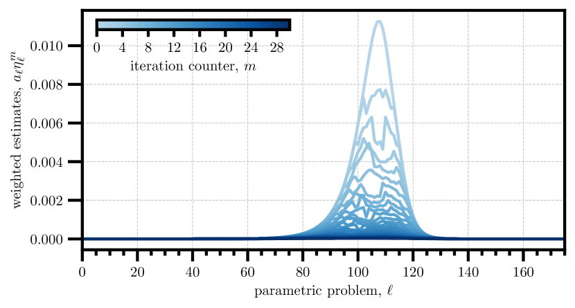
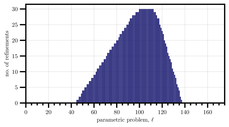
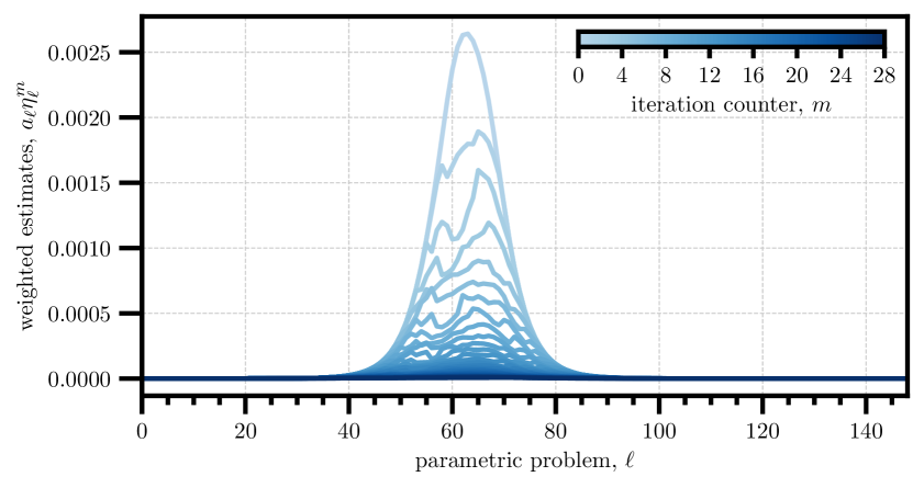
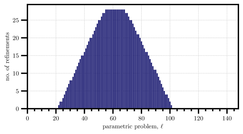
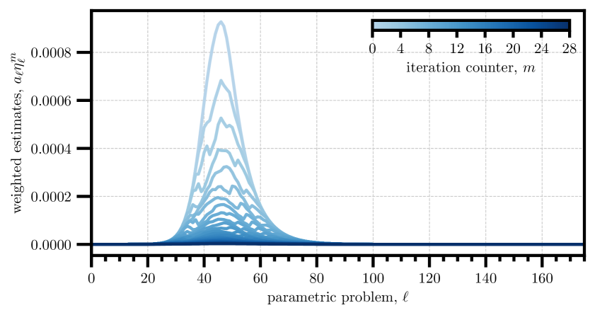
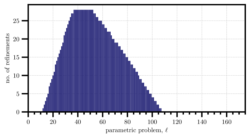
Figure 4. Test case II (multimesh setting; $s=0.3$ (top row), $s=0.5$ (middle row), and $s=0.7$ (bottom row)): the number of refinements for each mesh $\mathcal{T}_{l}$ ($l=1,\ldots,N$) (right column) and the corresponding weighted error estimates $a_{l}\eta_{l}^{m}$ (see (25)) (left column). In the left column, different shades represent different iterations $m$ of the adaptive loop.

Finally, for $s=0.3$, Figure 5 depicts the initial coarse mesh $\mathcal{T}^{0}$, the examples of finite element meshes generated at the 19th iteration the adaptive multimesh refinement algorithm for some parametric problems, and the corresponding union mesh.

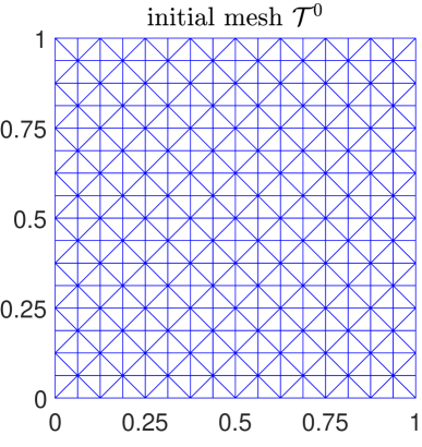
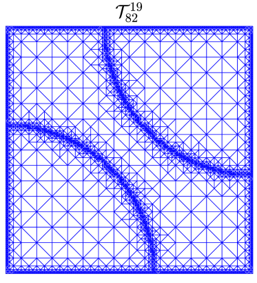
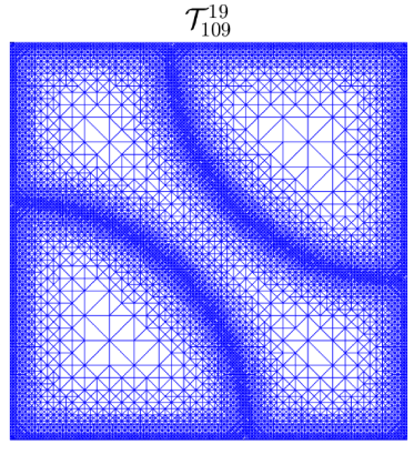
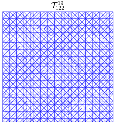
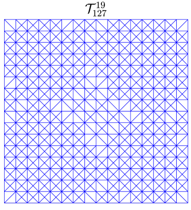
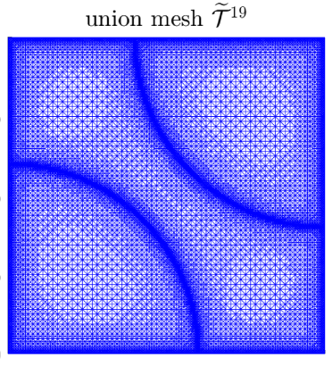
Figure 5. Test case II (multimesh setting; $s=0.3$): the initial coarse mesh $\mathcal{T}^{0}$; finite element meshes $\mathcal{T}_{l}^{m}$ generated by Algorithm 1 ($m=19$; $l=82,\,109,\,122,\,127$); the union mesh $\widetilde{\mathcal{T}}^{19}$.

6.3. Test case III: L-shaped domain

We now set $f\equiv 1$ and look to solve the model problem (1) on the L-shaped domain $\Omega=(-1,1)^{2}\setminus(-1,0]^{2}$. In this case, the solution $u$ to problem (1) exhibits boundary layers as well as a geometric singularity at the domain’s reentrant corner. Therefore, the adaptive refinement strategy will need to capture the interplay of these two different types of singular behavior in the solution $u$.

In this test case, we use the initial mesh $\mathcal{T}^{0}$ as a uniform mesh of 384 right-angled triangles (see Figure 6). For each $s\in\{0.1,\,0.3,\,0.5,\,0.7,\,0.9\}$, we set the same tolerance as in test case II (see Table 2) and run our adaptive multimesh refinement algorithm. The decay rates for global a posteriori error estimates $\eta^{m}$ and $\widetilde{\eta}^{m}$ (see (27) and (30), respectively) as well as the theoretical convergence rates predicted in [12, Theorem 4.3] for uniform mesh refinement are given in Table 3.

$s$	0.1	0.3	0.5	0.7	0.9
$m_{*}$	39	34	33	35	40
decay rate for $\eta^{m}$	0.64	0.84	0.93	0.96	0.98
decay rate for $\widetilde{\eta}^{m}$	0.67	0.91	0.97	0.99	1.00
decay rate for uniform refinement	0.35	0.55	0.67	0.67	0.67

Table 3. Test case III (multimesh setting): the number $m_{*}$ of iterations and the decay rates for global error estimates $\eta^{m}$,  $\widetilde{\eta}^{m}$ as well as the theoretical convergence rates for uniform mesh refinement (see [12, Theorem 4.3]).

As in all previous test cases, we observe that the global error estimates $\eta^{m}$ based on the triangle inequality decay with a slower rate than the estimates $\widetilde{\eta}^{m}$ computed using union meshes. This conclusion once again confirms superior effectivity and robustness of the global error estimation strategy based on the union mesh. In all computations the decay rates for global error estimates $\eta^{m}$,  $\widetilde{\eta}^{m}$ generated by the adaptive algorithm exceed the rates predicted by [12, Theorem 4.3] for uniformly refined meshes. As expected, for $s=0.9$, the adaptive algorithm has recovered the optimal convergence rate, $\mathcal{O}\big{(}\mathrm{dof}^{-1}\big{)}$. We emphasize that this optimal rate cannot be achieved if uniform mesh refinement is used. This is due to the presence of dominant geometric singularity in the solution to problem (1) when $s$ is close to 1. We note that for $s=0.7$, the rate is also very close to optimal.

Figure 6 depicts the initial coarse mesh $\mathcal{T}^{0}$ as well as the union meshes generated at the 19th iteration of Algorithm 1 for $s\in\{0.1,\,0.3,\,0.5,\,0.7,\,0.9\}$. This figure shows how adaptive mesh refinement reflects the interplay of two types of singularities in the solution to problem (1) in this test case for different values of $s$, with strong refinement solely in the boundary layer for $s=0.1$ gradually transitioning towards strong refinement at the reentrant corner and barely any refinement in the boundary layer for $s=0.9$.

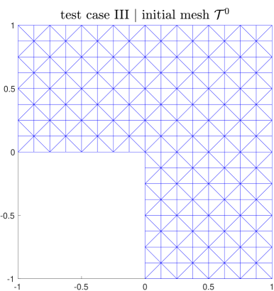
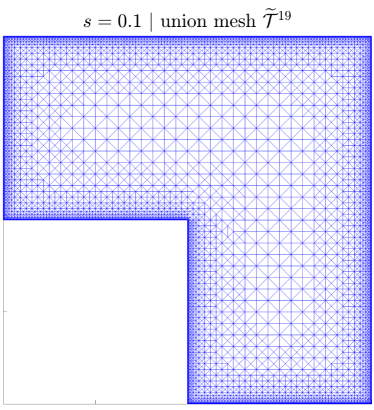
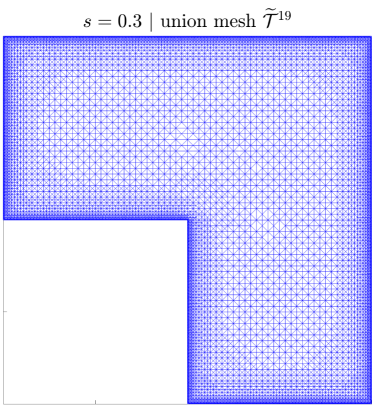
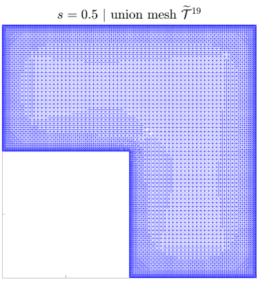
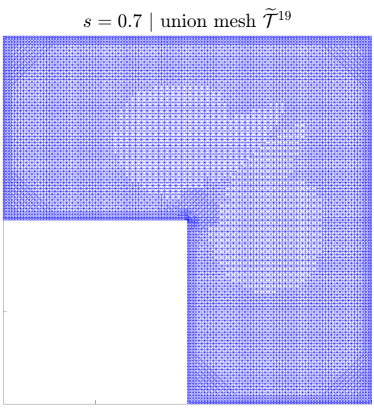
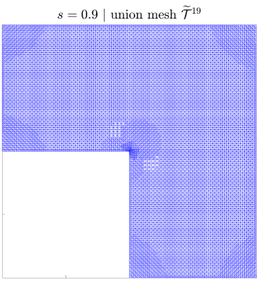
Figure 6. Test case III (multimesh setting): the initial coarse mesh $\mathcal{T}^{0}$; the union meshes $\widetilde{\mathcal{T}}^{19}$ generated by Algorithm 1 for $s\in\{0.1,\,0.3,\,0.5,\,0.7,\,0.9\}$.

7. Conclusions

The numerical solution of FPDEs presents many challenges due to the nonlocal nature of the underlying pseudo-differential operators. Adaptive solution strategies have the potential to significantly reduce computational times and achieve optimal convergence and complexity in the presence of sharp interfaces, boundary layers and geometric singularities in solutions to FPDEs.

Focusing on the spectral fractional Laplacian, an important contribution of this paper is in developing a novel multimesh rational approximation scheme for discretizing fractional powers of elliptic operators. The scheme comes with an effective a posteriori error estimation strategy driving an adaptive multimesh refinement algorithm that is implemented in the open-source MATLAB package T-IFISS. Extensive numerical experimentation has demonstrated the effectivity and robustness of the global error estimation strategy based on the union mesh, superior convergence rates for approximations generated by the adaptive algorithm compared to approximations obtained via uniform mesh refinement, and, crucially, a drastic reduction in computational complexity (measured in terms of the cumulative number of degrees of freedom) compared to that for adaptive single-mesh approximations.

In this work, adaptive approximations are generated on locally quasi-uniform finite element meshes. Therefore, the observed convergence rates for adaptive multimesh approximations are suboptimal in test cases with smaller fractional powers of the Laplacian. Optimal convergence rates can be recovered by employing anisotropic mesh refinement that captures singular behavior of the solution within boundary/interior layers more effectively than refinements that preserve shape-regularity of meshes. An extension of the multimesh approach proposed in this paper to anisotropic meshes, including a posteriori error estimation on anisotropic elements and, critically, a fully-adaptive anisotropic mesh refinement strategy will be the subject of future work.

References

- [1] M. Ainsworth and C. Glusa, Aspects of an adaptive finite element method for the fractional Laplacian: a priori and a posteriori error estimates, efficient implementation and multigrid solver, Comput. Methods Appl. Mech. Engrg., 327 (2017), pp. 4–35.
- [2] M. Ainsworth and J. T. Oden, A Posteriori Error Estimation in Finite Element Analysis, Pure Appl. Math. (N. Y.), Wiley, New York, 2000.
- [3] H. Antil, Y. Chen, and A. Narayan, Reduced basis methods for fractional Laplace equations via extension, SIAM J. Sci. Comput., 41 (2019), pp. A3552–A3575.
- [4] A. V. Balakrishnan, Fractional powers of closed operators and the semigroups generated by them, Pacific J. Math., 10 (1960), pp. 419–437.
- [5] L. Banjai, J. M. Melenk, R. H. Nochetto, E. Otárola, A. J. Salgado, and C. Schwab, Tensor FEM for spectral fractional diffusion, Found. Comput. Math., 19 (2019), pp. 901–962.
- [6] L. Banjai, J. M. Melenk, and C. Schwab, Exponential convergence of FEM for spectral fractional diffusion in polygons, Numer. Math., 153 (2023), pp. 1–47.
- [7] R. E. Bank and A. Weiser, Some a posteriori error estimators for elliptic partial differential equations, Math. Comp., 44 (1985), pp. 283–301.
- [8] A. Bespalov, L. Rocchi, and D. Silvester, T-IFISS: a toolbox for adaptive FEM computation, Comput. Math. Appl., 81 (2021), pp. 373–390.
- [9] A. Bonito, W. Lei, and J. E. Pasciak, The approximation of parabolic equations involving fractional powers of elliptic operators, J. Comput. Appl. Math., 315 (2017), pp. 32–48.
- [10] , Numerical approximation of space-time fractional parabolic equations, Comput. Methods Appl. Math., 17 (2017), pp. 679–705.
- [11] A. Bonito and M. Nazarov, Numerical simulations of surface quasi-geostrophic flows on periodic domains, SIAM J. Sci. Comput., 43 (2021), pp. B405–B430.
- [12] A. Bonito and J. E. Pasciak, Numerical approximation of fractional powers of elliptic operators, Math. Comp., 84 (2015), pp. 2083–2110.
- [13] , Numerical approximation of fractional powers of regularly accretive operators, IMA J. Numer. Anal., 37 (2017), pp. 1245–1273.
- [14] R. Bulle, O. Barrera, S. P. A. Bordas, F. Chouly, and J. S. Hale, An a posteriori error estimator for the spectral fractional power of the Laplacian, Comput. Methods Appl. Mech. Engrg., 407 (2023), pp. Paper No. 115943, 27.
- [15] E. Cancès, G. Dusson, Y. Maday, B. Stamm, and M. Vohralík, Guaranteed and robust a posteriori bounds for Laplace eigenvalues and eigenvectors: conforming approximations, SIAM J. Numer. Anal., 55 (2017), pp. 2228–2254.
- [16] C. Carstensen, A. Ern, and S. Puttkammer, Guaranteed lower bounds on eigenvalues of elliptic operators with a hybrid high-order method, Numer. Math., 149 (2021), pp. 273–304.
- [17] L. Chen, R. H. Nochetto, E. Otárola, and A. J. Salgado, A PDE approach to fractional diffusion: a posteriori error analysis, J. Comput. Phys., 293 (2015), pp. 339–358.
- [18] N. Cusimano, F. del Teso, L. Gerardo-Giorda, and G. Pagnini, Discretizations of the spectral fractional Laplacian on general domains with Dirichlet, Neumann, and Robin boundary conditions, SIAM J. Numer. Anal., 56 (2018), pp. 1243–1272.
- [19] M. D’Elia, Q. Du, C. Glusa, M. Gunzburger, X. Tian, and Z. Zhou, Numerical methods for nonlocal and fractional models, Acta Numer., 29 (2020), pp. 1–124.
- [20] W. Dörfler, A convergent adaptive algorithm for Poisson’s equation, SIAM J. Numer. Anal., 33 (1996), pp. 1106–1124.
- [21] M. Faustmann, J. M. Melenk, and D. Praetorius, Quasi-optimal convergence rate for an adaptive method for the integral fractional Laplacian, Math. Comp., 90 (2021), pp. 1557–1587.
- [22] S. Harizanov, R. Lazarov, S. Margenov, and P. Marinov, Numerical solution of fractional diffusion-reaction problems based on BURA, Comput. Math. Appl., 80 (2020), pp. 316–331.
- [23] M. Karkulik, D. Pavlicek, and D. Praetorius, On 2D newest vertex bisection: optimality of mesh-closure and -stability of -projection, Constr. Approx., 38 (2013), pp. 213–234.
- [24] N. Kopteva and E. O’Riordan, Shishkin meshes in the numerical solution of singularly perturbed differential equations, Int. J. Numer. Anal. Model., 7 (2010), pp. 393–415.
- [25] A. Lischke, G. Pang, M. Gulian, and et al., What is the fractional Laplacian? A comparative review with new results, J. Comput. Phys., 404 (2020), pp. 109009, 62.
- [26] R. H. Nochetto, E. Otárola, and A. J. Salgado, A PDE approach to fractional diffusion in general domains: a priori error analysis, Found. Comput. Math., 15 (2015), pp. 733–791.
- [27] D. J. Silvester, A. Bespalov, Q. Liao, and L. Rocchi, Triangular IFISS (T-IFISS). Available online at http://www.manchester.ac.uk/ifiss/tifiss, February 2019.
- [28] R. Stevenson, The completion of locally refined simplicial partitions created by bisection, Math. Comp., 77 (2008), pp. 227–241.
- [29] P. N. Vabishchevich, Approximation of a fractional power of an elliptic operator, Numer. Linear Algebra Appl., 27 (2020), pp. e2287, 14.
- [30] R. Verfürth, A posteriori error estimation and adaptive mesh-refinement techniques, J. Comput. Appl. Math., 50 (1994), pp. 67–83.
- [31] X. Zhao, X. Hu, W. Cai, and G. E. Karniadakis, Adaptive finite element method for fractional differential equations using hierarchical matrices, Comput. Methods Appl. Mech. Engrg., 325 (2017), pp. 56–76.