Eigen-inference by Marchenko-Pastur inversion

Abstract

A new formula for Marchenko-Pastur inversion is derived and used for inference of population linear spectral statistics. The formula allows for estimation of the Stieltjes transform of the population spectral distribution $\bm{s}_{H}(z)$, when $z$ is sufficiently far from the support of the population spectral distribution $H$. If the dimension $d$ and the sample size $n$ go to infinity simultaneously such that $\frac{d}{n}\rightarrow c>0$, the estimation error is shown to be asymptotically less than $\frac{n^{\varepsilon}}{n}$ for arbitrary $\varepsilon>0$. By integrating along a curve around the support of $H$, estimators for population linear spectral statistics are constructed, which benefit from this convergence speed of $\frac{n^{\varepsilon}}{n}$.

1 Introduction

Estimating the covariance matrix $\Sigma_{n}$ of a multivariate distribution $\mathcal{P}$ on $\mathbb{R}^{d}$ from samples $Y_{1},...,Y_{n}$ of iid vectors is a fundamental question in statistics. The sample covariance matrix

$$\bm{S}_{n}:=\bigg{(}\frac{1}{n}\sum\limits_{k=1}^{n}(Y_{k})_{i}(Y_{k})_{j}\bigg{)}_{i,j\in\{1,...,d\}}$$

performs well only, when the dimension $d$ is much smaller than the sample size $n$. For comparable dimension and sample size, i.e. when $d,n\rightarrow\infty$ such that

$$c_{n}:=\frac{d}{n}\rightarrow c_{\infty}>0\ ,$$ (1.1)

the celebrated Marchenko-Pastur law, as discovered in the Gaussian case by [MP_original], describes how the eigenvalues of $\bm{S}_{n}$ will asymptotically behave, for given $\Sigma_{n}$. More precisely, under the convergence of measures

$$H_{n}:=\frac{1}{d}\sum\limits_{j=1}^{d}\delta_{\lambda_{j}(\Sigma_{n})}\xRightarrow{n\rightarrow\infty}H_{\infty}$$ (1.2)

to a probability measure with compact support on $[0,\infty)$ the Marchenko-Pastur law gives the convergence

$$1=\mathbb{P}\Big{(}\hat{\nu}_{n}:=\frac{1}{d}\sum\limits_{j=1}^{d}\delta_{\lambda_{j}(\bm{S}_{n})}\xRightarrow{n\rightarrow\infty}\nu_{\infty}\Big{)}$$ (1.3)

to a deterministic limiting spectral distribution (LSD) $\nu_{\infty}$ derived from $H_{\infty}$ and $c_{\infty}$ by the so called Marchenko-Pastur equation. The Marchenko-Pastur equation is formulated in forms of Stieltjes transforms $\bm{s}_{\mu}$ of measures $\mu$ on $\mathbb{R}$, which are defined as maps

$$\bm{s}_{\mu}:\mathbb{C}^{+}\equiv\{z\in\mathbb{C}\mid\operatorname{Im}(z)>0\}\rightarrow\mathbb{C}^{+}\ \ ;\ \ z\mapsto\int_{\mathbb{R}}\frac{1}{\lambda-z}\,d\mu(\lambda)\ .$$ (1.4)

The Stieltjes transform $\bm{s}_{\mu}$ uniquely identifies the underlying probability measure $\mu$ on $\mathbb{R}$ and the value of $\bm{s}_{\mu}(z)$ for $z$ close to $\mathbb{R}$ is especially significant for reconstructing $\mu$, since $\frac{1}{\pi}\operatorname{Im}(\bm{s}_{\mu}(x+i\eta))$ is by construction the integral over the kernel $\frac{\eta/\pi}{(\bullet-x)^{2}+\eta^{2}}$ with regards to $\mu$. The Marchenko-Pastur equation in the formulation from page 556 of [BaiCLT] is then as follows.

Lemma 1.1 (Marchenko-Pastur equation).

Lemma_MP 
For any probability measure $H$ on $[0,\infty)$ with compact support and constant $c>0$, there exists a probability measure $\nu$ on $[0,\infty)$ with compact support that is uniquely defined by the following property of its Stieltjes transform $\bm{s}_{\nu}$.

For all $\tilde{z}\in\mathbb{C}^{+}$ the Stieltjes transform $\bm{s}_{\nu}(\tilde{z})$ is the unique solution to

$$s=\int_{\mathbb{R}}\frac{1}{\lambda(1-c\tilde{z}s-c)-\tilde{z}}\,dH(\lambda)$$ (1.5)

in the set

$$\tilde{Q}_{\tilde{z},c}:=\Big{\{}s\in\mathbb{C}\ \Big{|}\ \operatorname{Im}\Big{(}cs+\frac{c-1}{\tilde{z}}\Big{)}>0\Big{\}}\ .$$ (1.6)

The Marchenko-Pastur equation can be solved numerically by iterating the operator

$$T_{\tilde{z},H,c}(s)=\int_{\mathbb{R}}\frac{1}{\lambda(1-c\tilde{z}s-c)-\tilde{z}}\,dH(\lambda)$$

until an approximate fixed point $s\approx T_{\tilde{z},H,c}(s)$ is found, which leads to highly accurate predictions of the spectral distributions $\hat{\nu}_{n}$ (see Figure 1).

$c_{n}=1$            $c_{n}=1$           $c_{n}=0.5$           $c_{n}=0.1$

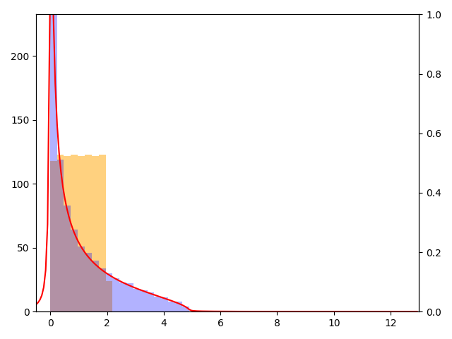
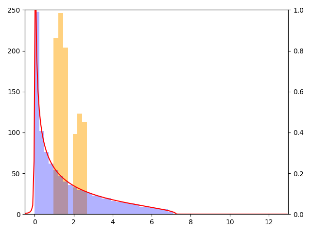
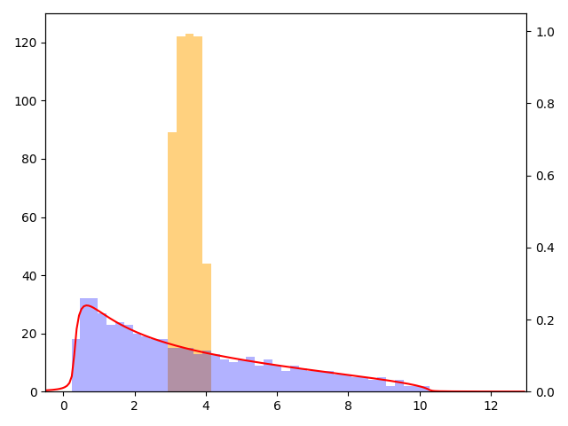
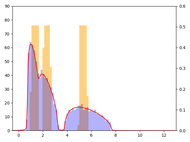
Figure 1: Histograms of $H_{n}$ (orange) and corresponding $\hat{\nu}_{n}$ (blue) for $d=1000$.
The prediction $x\mapsto\frac{1}{\pi}\operatorname{Im}(\bm{s}_{\nu_{n}}(x+i\eta))$ for $\eta=\frac{1}{200}$ and $\nu_{n}$ derived from $H_{n},c_{n}$ as in Lemma LABEL:Lemma_MP is marked red.

This paper describes a new method of Marchenko-Pastur inversion, i.e. reconstruction of $H$ (or $\bm{s}_{H}$) from $\nu$ and $c$. Specifically, we in Lemma LABEL:Lemma_MPInversion show that $\bm{s}_{H}(z)$ is for all $z\in\mathbb{C}^{+}$ with

$$\operatorname{Im}\big{(}(1-cz\bm{s}_{H}(z)-c)z\big{)}>0\ \ \text{ and }\ \ \Big{|}\frac{cz\operatorname{Im}(z\bm{s}_{H}(z))}{\operatorname{Im}((1-cz\bm{s}_{H}(z)-c)z)}\Big{|}<1$$ (1.7)

the unique solution to

$$zs+1=\int_{\mathbb{R}}\frac{\lambda}{\lambda-(1-czs-c)z}\,d\nu(\lambda)$$ (1.8)

from the set

$$\Big{\{}s\in\mathbb{C}^{+}\ \Big{|}\ \operatorname{Im}((1-czs-c)z)>0,\,\Big{|}\frac{cz\operatorname{Im}(zs)}{\operatorname{Im}((1-czs-c)z)}\Big{|}<1\Big{\}}\ .$$

The conditions (1.7) amount to $z\in\mathbb{C}^{+}$ being sufficiently far away from the support of $H$ (see Figure 2). The distribution of $H$ can thus not be easily recovered by examining $x\mapsto\frac{1}{\pi}\operatorname{Im}(\bm{s}_{H}(x+i\eta))$ for small $\eta>0$ (similar to Figure 1), since for $x$ near the support of $H$ and small $\eta>0$ the point $z=x+i\eta$ will be too close to $\operatorname{supp}(H)$ for (1.7) to hold and the inversion formula (1.8) will not grant $\bm{s}_{H}(x+i\eta)$.

Instead, $H$ can be recovered by the fact that for any holomorphic function $f:\mathbb{C}\rightarrow\mathbb{C}$ we by Cauchy’s integral formula have

$$\int_{\mathbb{R}}f(\lambda)\,dH(\lambda)=\frac{1}{2\pi i}\oint_{\gamma}f(z)\int_{\mathbb{R}}\frac{1}{\lambda-z}\,dH(\lambda)\,dz$$

$$=\frac{1}{2\pi i}\oint_{\gamma\cap\mathbb{C}^{+}}\big{(}f(z)\bm{s}_{H}(z)-f(\overline{z})\overline{\bm{s}_{H}(z)}\big{)}\,dz\ ,$$ (1.9)

where $\gamma$ is a closed curve going clockwise around $\operatorname{supp}(H)$ and $\gamma\cup\mathbb{C}^{+}$ is the part of $\gamma$, which stays on $\mathbb{C}^{+}$. If the curve $\gamma\cap\mathbb{C}^{+}$ stays sufficiently far away from $\operatorname{supp}(H)$ that (1.7) holds for all $z$ on its path, then the inversion formula (1.8) yields each $\bm{s}_{H}(z)$ needed for the integral (1) and we have reconstructed $\int_{\mathbb{R}}f(\lambda)\,dH(\lambda)$ from $\nu$ and $c$.

While Section 2 will deal with the proof of the Marchenko-Pastur inversion formula and its robustness under perturbations of $\nu$, Sections 3 and 4 will be dedicated to applying this idea to eigen-inference, in the sense that we estimate $\bm{s}_{H_{n}}$, $\int_{\mathbb{R}}f(\lambda)\,dH_{n}(\lambda)$ and even the eigenvalues of $\Sigma_{n}$ themselves from the observable objects $c_{n}$ and $\hat{\nu}_{n}$.

$c=0.1$, $H=\frac{1}{2}\delta_{\frac{1}{2}}+\frac{1}{2}\delta_{1}$      $c=0.5$, $H=\frac{1}{2}\delta_{\frac{1}{2}}+\frac{1}{2}\delta_{1}$       $c=0.1$, $H=\operatorname{Unif}([0,1])$        $c=0.5$, $H=\operatorname{Unif}([0,1])$

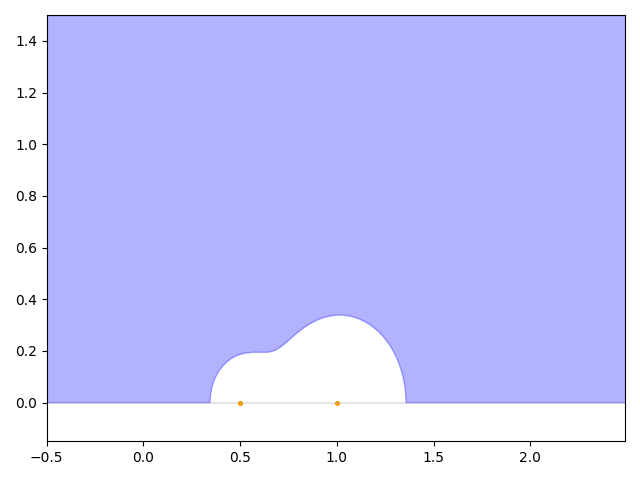
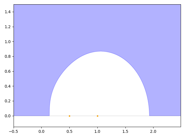
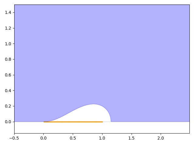
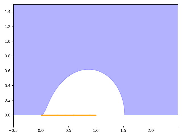
Figure 2: Graphical representations of the set of all $z\in\mathbb{C}^{+}$ which satisfy (1.7). The sets are colored blue and the supports of $H$ are marked orange.

1.1 Marchenko-Pastur laws

Let $(d_{n})_{n\in\mathbb{N}}$ be a sequence with values in $\mathbb{N}$ such that the quotient $\frac{d_{n}}{n}$ converges to a constant $c>0$. Suppressing the dependence of $d_{n}$ on $n$ in our notation we write

$$c_{n}:=\frac{d}{n}\rightarrow c_{\infty}>0\ .$$

A fundamental assumption of random matrix theory is the existence of a deterministic $(d\times\tilde{d})$ matrix $T_{n}$ and a random $(\tilde{d}\times n)$ matrix $\bm{X}_{n}$ with independent centered entries, each with variance one, such that

$$\bm{Y}_{n}=T_{n}\bm{X}_{n}\ .$$ (1.10)

The matrix $T_{n}$ must by construction satisfy $T_{n}T_{n}^{*}=\Sigma_{n}$ and the sample covariance matrix is defined as

$$\bm{S}_{n}:=\frac{1}{n}\bm{Y}_{n}\bm{Y}_{n}^{*}=\frac{1}{n}T_{n}\bm{X}_{n}\bm{X}_{n}^{*}T_{n}^{*}\ .$$

Assuming the population spectral distribution

$$H_{n}:=\frac{1}{d}\sum\limits_{j=1}^{d}\delta_{\lambda_{j}(\Sigma_{n})}$$

converges weakly to some limiting distribution $H_{\infty}$ with compact support on $[0,\infty)$, the Marchenko-Pastur law - as we have already stated in (1.3) - almost surely gives the weak convergence of the empirical spectral distribution (ESD)

$$\hat{\nu}_{n}:=\frac{1}{d}\sum\limits_{j=1}^{d}\delta_{\lambda_{j}(\bm{S_{n}})}$$

to the LSD $\nu_{\infty}$ itself with compact support on $[0,\infty)$. The first proof of the Marchenko-Pastur law for $T_{n}=\operatorname{Id_{d}}$ and $X_{i,j}\sim\mathcal{N}(0,1)$ was given in 1967 by Marchenko and Pastur in [MP_original]. The generalization to arbitrary iid entries of $\bm{X}_{n}$ that are centered with variance one was achieved in [MP_Yin] under mild conditions on $H_{n}$. The limiting spectral distribution of $A+\frac{1}{n}\bm{X}_{n}^{*}\mathbb{T}\bm{X}_{n}$ for a deterministic matrix $A$ and possibly non-positive-definite $\mathbb{T}$ was first characterized in [MP_Bai]. The assumption of independence between rows of $\bm{X}_{n}$ was weakened in [MP_RowCorrelation_Bai] and in the isotropic case $T_{n}=\operatorname{Id}_{d}$ [MP_Heiny] even allows correlations between rows and columns of $\bm{X}_{n}$ provided they go to zero sufficiently quickly with $n\rightarrow\infty$. A series of papers [MP_NessSuff_Yaskov], [MP_NessSuff_Nina] and [MP_NessSuff_Yao] deals with necessary and sufficient conditions for the Marchenko-Pastur law to hold in the isotropic case. The recent paper [StrongMP] loosens the assumption (1.10) and the data matrix $\bm{Y}_{n}$ is allowed to have more general independent columns, while still assuming the covariance matrices of said columns to be simultaneously diagonalizable. Marchenko-Pastur laws for the setting of dependent columns arising from high-dimensional time series are studied in the papers [TimeMP1, TimeMP2, TimeMP3, TimeMP4, TimeMPLast].

Marchenko-Pastur laws have also been generalized into so-called local laws, where the behavior of $\bm{s}_{\hat{\nu}_{n}}(z)$ is described depending on how close $z$ is to certain parts of the support of the LSD $\nu_{\infty}$. This allows for more detailed analysis of eigenvalues at the edge of the spectrum, such as largest or smallest eigenvalues. The most influential and comprehensive works on local laws in the setting described here are [BloemendalIsotropicLocalLaws] and [KnowlesAnisotropicLocalLaws]. The articles [LocalLargestEV_Bloemendal] and [LocalLargestEVSchnelli] apply the theory of local laws to the analysis of principal components and the Tracy-Widom law.

1.2 Spectral CLTs

A well-known effect of high-dimensional random matrix theory are fast convergence rates of order $\frac{1}{n}$ instead of $\frac{1}{\sqrt{n}}$. Similarly to the standard central limit theorem (CLT) one can for a measurable function $f:\mathbb{R}\rightarrow\mathbb{R}$ observe the difference between the empirical integral $\int_{\mathbb{R}}f\,d\hat{\nu}_{n}$ and the limiting integral $\int_{\mathbb{R}}f\,d\nu_{\infty}$. Spectral central limit theorems (spectral CLTs) describe the weak convergence of

$$n\Big{(}\int_{\mathbb{R}}f\,d\hat{\nu}_{n}-\int_{\mathbb{R}}f\,d\nu_{\infty}\Big{)}$$

to Gaussian distributions. The earliest spectral CLT for the setting $T_{n}=\operatorname{Id_{d}}$ and $X_{i,j}\sim\mathcal{N}(0,1)$ goes back to 1982 by Jonsson in [JonssonCLT]. In the celebrated paper [BaiCLT] Bai and Silverstein first formulated a spectral CLT for general $\Sigma_{n}$ and $T_{n}=\Sigma_{n}^{\frac{1}{2}}$ in the case where the entries of $\bm{X}_{n}$ are iid and have fourth moment equal to a standard normal distribution. The latter condition was removed and the class of functions $f$ for which the CLT holds was expanded by Najim and Yao in [NajimYao]. In the paper [CLTniceCov] better formulas for the limiting mean and covariance are given. Generalizations of the spectral CLT to the case $\frac{d}{n}\rightarrow\infty$ or to columns generated from a high-dimensional time series were done in [DetteSequential] and [YaoUltraCLT].

Defining an $n$-wise version $\nu_{n}$ of the limiting spectral distribution $\nu_{\infty}$ allows these local laws and spectral CLTs to be independent of the speed of the convergences

$$c_{n}=\frac{d}{n}\rightarrow c_{\infty}\ \ \text{ and }\ \ H_{n}\xRightarrow{n\rightarrow\infty}H_{\infty}\ .$$

The distribution $\nu_{n}$ is obtained from $H_{n}$ and $c_{n}$ through the Marchenko-Pastur equation (see Lemma LABEL:Lemma_MP) analogous to how $\nu_{\infty}$ is obtained from $H_{\infty}$ and $c_{\infty}$.

We will also use $\hat{\underline{\nu}}_{n}$ and $\underline{\nu}_{n}$ to denote the probability measures

$$\hat{\underline{\nu}}_{n}=\frac{1}{n}\sum\limits_{j=1}^{n}\delta_{\lambda_{j}(\frac{1}{n}\bm{X}_{n}^{*}\Sigma_{n}\bm{X}_{n})}=(1-c_{n})\delta_{0}+c_{n}\hat{\nu}_{n}\ \ \text{ and }\ \ \underline{\nu}_{n}=(1-c_{n})\delta_{0}+c_{n}\nu_{n}\ .$$ (1.11)

The corresponding Stieltjes transforms clearly satisfy

$$\bm{s}_{\hat{\underline{\nu}}_{n}}(z)=\frac{1-c_{n}}{-z}+c_{n}\bm{s}_{\hat{\nu}_{n}}(z)\ \ \text{ and }\ \ \bm{s}_{\underline{\nu}_{n}}(z)=\frac{1-c_{n}}{-z}+c_{n}\bm{s}_{\nu_{n}}(z)\ .$$ (1.12)

1.3 Eigen-inference

In practice, one is often interested in estimating the underlying population covariance $\Sigma_{n}$, but only has access to the data-matrix $\bm{Y}_{n}$ and by extension the sample covariance matrix $\bm{S}_{n}=\frac{1}{n}\bm{Y}_{n}\bm{Y}_{n}^{*}$ as well as its spectral distribution $\hat{\nu}_{n}$. In order for an estimator of $\Sigma_{n}$ to be rotation-equivariant, it was noted in [LedoitWolf1] that it must have the same eigenvectors as $\bm{S}_{n}$. The problem of estimating $\Sigma_{n}$ in a rotation-equivariant manner reduces to estimation of the population eigenvalues. The theoretical process of recovering the population spectral measure $H_{n}$ from $\nu_{n}$ (which is assumed to be close to $\hat{\nu}_{n}$) is called Marchenko-Pastur inversion, while finding algorithms for the construction of estimators for $\Sigma_{n}$ from $\bm{Y}_{n}$ is called eigen-inference. Let

$$\bm{S}_{n}=U_{n}\,\operatorname{diag}\big{(}\lambda_{1}(\bm{S}_{n}),...,\lambda_{d}(\bm{S}_{n})\big{)}\,U_{n}^{*}$$

be the spectral decomposition of the sample covariance matrix, then estimators of the form

$$\hat{\Sigma}_{n,\varphi}=U_{n}\,\operatorname{diag}\big{(}\varphi(\lambda_{1}(\bm{S}_{n})),...,\varphi(\lambda_{d}(\bm{S}_{n}))\big{)}\,U_{n}^{*}$$ (1.13)

are called shrinkage estimators for the population covariance matrix.

An early work on Marchenko-Pastur inversion by solving a convex optimization problem is [MPIKaroui]. El Karoui proves consistency of the resulting estimator $\hat{H}_{n}$ in the sense $1=\mathbb{P}\big{(}\hat{H}_{n}\xRightarrow{n\rightarrow\infty}H_{\infty}\big{)}$, but gives no bounds for the rate of convergence. In [MPIBaiYao] Bai, Chen and Yao construct a moment based estimator under the assumption $H_{\infty}=t_{1}\delta_{\theta_{1}}+...+t_{k}\delta_{\theta_{k}}$ for the parameters $(t_{1},...,t_{k},\theta_{1},...,\theta_{k})$. They were also able to show asymptotic normality of the estimation error with rate $\frac{1}{n}$. Further work on parametric models of this type was done in [MPILiBaiYao].

The papers [LedoitWolf1] and [LedoitWolf2] present an algorithm for discrete Marchenko-Pastur inversion, which they use to define a consistent estimator for $\Sigma_{n}$ in the sense

$$\frac{1}{d}\sum\limits_{i=1}^{d}\big{(}\hat{\lambda_{j}-\lambda_{j}(\Sigma_{n})}\big{)}^{2}\xrightarrow{n\rightarrow\infty}_{a.s.}0\ .$$

Their estimator is also the solution of an optimization problem built upon the discretization.Ledoit and Wolf’s method and its extensions are widely regarded as state of the art in high-dimensional population eigenvalue estimation.

A less well known - though mathematically very satisfying - approach to eigen-inference was introduced by Kong and Valiant in [MPIKong]. They make the observation that for every list of $k$ distinct integers $\sigma_{1},...,\sigma_{k}\in\{1,...,n\}$ the mean

$$\mathbb{E}\bigg{[}\prod\limits_{i=1}^{k}(\bm{Y}_{n}^{*}\bm{Y}_{n})_{\sigma_{i},\sigma_{(i\,\operatorname{mod}\,k)+1}}\bigg{]}$$

is equal to $\sum\limits_{j=1}^{d}\lambda_{j}(\Sigma_{n})^{k}=\operatorname{tr}(\Sigma_{n}^{k})=H_{n}(\bullet^{k})$. Unfortunately, the product in the mean has very high variance, so they must average over many different lists $(\sigma_{1},...,\sigma_{k})$ to get a consistent estimator of the population moments $H_{n}(\bullet^{k})$. While the resulting estimators are computationally costly to calculate, Kong and Valiant were able to prove error bounds with rates dependent on $k$, but no better than $\frac{1}{\sqrt{n}}$.

1.4 Our contributions

The first contribution of this paper is that we find a non-explicit solution of the Marchenko-Pastur equation, that provides an elegant method of Marchenko-Pastur inversion. We show in Lemma LABEL:Lemma_MPInversion that for all $z\in\mathbb{C}^{+}$ - with a certain distance to the support of $H$ - the Stieltjes transform $\bm{s}_{H}(z)$ is the unique solution to

$$zs+1=\int_{\mathbb{R}}\frac{\lambda}{\lambda-(1-czs-c)z}\,d\nu(\lambda)\ .$$ (1.14)

We proceed to show in Theorem LABEL:Thm_EstimatorStieltjes that the empirical version of equation (1.14), i.e.

$$z\hat{s}+1=\int_{\mathbb{R}}\frac{\lambda}{\lambda-(1-cz\hat{s}-c)z}\,d\hat{\nu}_{n}(\lambda)$$

(for $z$ far enough away from $\operatorname{supp}(H_{n})$ and not too close to the real line) with high probability admits exactly one solution $\hat{s}_{n}(z)$, which will then be close to the true population Stieltjes transform $\bm{s}_{H_{n}}(z)$ in the sense $|\hat{s}_{n}(z)-\bm{s}_{H_{n}}(z)|\leq\frac{n^{\tilde{\varepsilon}}}{|z|n}$ for any $\tilde{\varepsilon}>0$.

Using this population Stieltjes transform estimator $\hat{s}_{n}(z)$ we can then for any holomorphic function $f:\mathbb{C}\rightarrow\mathbb{C}$ define an estimator $\hat{L}_{n}(f)$ (see 4.6) for the population linear spectral statistic

$$L_{H_{n}}(f)=\int_{\mathbb{R}}f\,dH=\frac{1}{d}\sum\limits_{j=1}^{d}\lambda_{j}(\Sigma_{n})\ .$$

In Theorem 4.1 we prove that $\big{|}\hat{L}_{n}(f)-L_{H_{n}}(f)\big{|}\leq\frac{n^{\tilde{\varepsilon}}}{n}$ in high probability for any $\tilde{\varepsilon}>0$.

Finally, in Definition 4.2 we define estimators for the population eigenvalues, that benefit from this fast convergence rate of almost $\frac{1}{n}$. Similarly to the estimators constructed in [MPIKaroui] or [LedoitWolf2], we define our estimator $\hat{w}_{n}$ of the eigenvalue-vector $\big{(}\lambda_{1}(\Sigma_{n}),...,\lambda_{d}(\Sigma_{n})\big{)}^{T}$ as a global minimizer to a loss function.

1.5 Assumptions

As stated in the Subsection 1.1, we assume that the sample covariance matrix is of the form

$$\bm{S}_{n}=\frac{1}{n}T_{n}\bm{X}_{n}\bm{X}_{n}^{*}T_{n}^{*}$$ (1.15)

for a $(d\times d)$-matrix $T_{n}$ with $T_{n}T_{n}^{*}=\Sigma_{n}$. Two standard assumptions to random matrix theory are that we are in the asymptotic regime

$$c_{n}=\frac{d}{n}\rightarrow c_{\infty}\ ,$$ (1.16)

while the entries of $\bm{X}_{n}$ are independent and satisfy

$$\mathbb{E}[(\bm{X}_{n})_{i,j}]=0\ \ \text{ and }\ \ \mathbb{E}[|(\bm{X}_{n})_{i,j}|^{2}]=1\ .$$ (1.17)

We also work under the base assumption that the weak convergence

$$H_{n}\xRightarrow{n\rightarrow\infty}H_{\infty}$$ (1.18)

holds for a limiting distribution

$$H_{\infty}\neq\delta_{0}$$ (1.19)

and that there exists a constant $\sigma^{2}>0$ such that

$$\forall n\in\mathbb{N}:\ ||\Sigma_{n}||\leq\sigma^{2}\ .$$ (1.20)

Finally, we assume uniformly bounded moments in the sense that for every $p\in\mathbb{N}$ there exists a $C_{p}>0$ such that

$$\forall n\in\mathbb{N},\,i\leq d,\,j\leq n:\ \mathbb{E}\big{[}|(\bm{X}_{n})_{i,j}|^{p}\big{]}\leq C_{p}\ .$$ (1.21)

2 Marchenko-Pastur inversion

This section deals with the relationship between $H$ and $\nu$ as defined in Lemma LABEL:Lemma_MP. By definitions of $\nu_{\infty},\nu_{n}$ the pairs $(H_{\infty},\nu_{\infty})$ and $(H_{n},\nu_{n})$ for all $n\in\mathbb{N}$ have this exact relationship. Assumptions (1.19) and 1.20 allow us to work under

$$H\neq\delta_{0}\ \ \text{ and }\ \ \operatorname{supp}(H)\subset[0,\sigma^{2}]$$ (2.1)

since $H_{n}$ will satisfy this for all large $n\in\mathbb{N}\cap\{\infty\}$.

We list some well-known properties of $\nu$, that follow from the much studied relationship of $(H_{\infty},\nu_{\infty})$. The mass of $\nu$ at zero is

$$\nu(\{0\})=\max\Big{(}\frac{c-1}{c},H(\{0\})\Big{)}\ .$$ (2.2)

The measure $\nu^{\prime}:=\nu-\delta_{0}\nu(\{0\})$ has continuous Lebesgue density on $(0,\infty)$. The assumption (2.1) implies

$$\operatorname{supp}(\nu)\subset[0,\sigma^{2}(1+\sqrt{c})^{2}]\ .$$ (2.3)

Coming to our main contribution to the field of Marchenko-Pastur inversion, we will first need to define some sets.

Definition 2.1 (Domains on $\mathbb{C}^{+}$).

Dependent on $H$ and $c$ for any $\varepsilon,\theta>0$ define the sets

$$\mathbb{D}_{H,c}(\varepsilon,\theta) :=\Big{\{}z\in\mathbb{C}^{+}\ \Big{|}\ \operatorname{Im}\big{(}(1-cz\bm{s}_{H}(z)-c)z\big{)}\geq\varepsilon,\Big{|}\frac{cz\operatorname{Im}(z\bm{s}_{H}(z))}{\operatorname{Im}((1-cz\bm{s}_{H}(z)-c)z)}\Big{|}\leq\theta\Big{\}}$$ (2.4)

$$\mathbb{Q}_{z,c}(\varepsilon,\theta) :=\Big{\{}s\in\mathbb{C}^{+}\ \Big{|}\ \operatorname{Im}((1-czs-c)z)\geq\varepsilon,\,\Big{|}\frac{cz\operatorname{Im}(zs)}{\operatorname{Im}((1-czs-c)z)}\Big{|}\leq\theta\Big{\}}\ .$$ (2.5)

We will also allow the inputs $0_{+}$ for $\varepsilon$ and $1_{-}$ or $\infty$ for $\theta$, by which we mean

$$\mathbb{D}_{H,c}(0_{+},\theta)=\bigcup\limits_{\varepsilon>0}\mathbb{D}_{H,c}(\varepsilon,\theta)$$

$$\hskip 28.45274pt=\Big{\{}z\in\mathbb{C}^{+}\ \Big{|}\ \operatorname{Im}\big{(}(1-cz\bm{s}_{H}(z)-c)z\big{)}>0,\Big{|}\frac{cz\operatorname{Im}(z\bm{s}_{H}(z))}{\operatorname{Im}((1-cz\bm{s}_{H}(z)-c)z)}\Big{|}\leq\theta\Big{\}}$$

and

$$\mathbb{D}_{H,c}(\varepsilon,\infty):=\bigcup\limits_{\theta>0}\mathbb{D}_{H,c}(\varepsilon,\theta)=\Big{\{}z\in\mathbb{C}^{+}\ \Big{|}\ \operatorname{Im}\big{(}(1-cz\bm{s}_{H}(z)-c)z\big{)}\geq\varepsilon\Big{\}}$$

$$\mathbb{D}_{H,c}(\varepsilon,1_{-}):=\bigcup\limits_{0<\theta<1}\mathbb{D}_{H,c}(\varepsilon,\theta)$$

$$\hskip 28.45274pt=\Big{\{}z\in\mathbb{C}^{+}\ \Big{|}\ \operatorname{Im}\big{(}(1-cz\bm{s}_{H}(z)-c)z\big{)}\geq\varepsilon,\Big{|}\frac{cz\operatorname{Im}(z\bm{s}_{H}(z))}{\operatorname{Im}((1-cz\bm{s}_{H}(z)-c)z)}\Big{|}<1\Big{\}}\ .$$

The definition of $\mathbb{Q}_{z,c}(0_{+},1_{-})$ is analogous.

The following Lemma is a surprisingly simple consequence of the Marchenko-Pastur equation, though it is not simply a reformulation of said equation, as was used by [MPIKaroui] to perform eigen-inference. Instead, it provides a semi-explicit solution to the Marchenko-Pastur equation, in the sense that (2.8) gives an explicit formula for $\bm{s}_{\nu}$ not at $z$ itself, but at the position $(1-cz\bm{s}_{H}(z)-c)z\in\mathbb{C}^{+}$.

Lemma 2.2 (Marchenko-Pastur inversion).

Lemma_MPInversion 
Assume $H\neq\delta_{0}$. For every $z\in\mathbb{D}_{H,c}(0_{+},\infty)$ it holds that

$$z\bm{s}_{H}(z)+1=\int_{\mathbb{R}}\frac{\lambda}{\lambda-(1-cz\bm{s}_{H}(z)-c)z}\,d\nu(\lambda)$$ (2.6)

and for every $z\in\mathbb{D}_{H,c}(0_{+},1_{-})$ the Stieltjes transform $\bm{s}_{H}(z)$ is the unique solution to

$$zs+1=\int_{\mathbb{R}}\frac{\lambda}{\lambda-(1-czs-c)z}\,d\nu(\lambda)$$ (2.7)

from the set $\mathbb{Q}_{z,c}(0_{+},1_{-})$.

Proof.

By re-arrangement and the definition of $\bm{s}_{\nu}$ one can see that (2.6) is equivalent to

$$\frac{\bm{s}_{H}(z)}{1-cz\bm{s}_{H}(z)-c}=\bm{s}_{\nu}\big{(}(1-cz\bm{s}_{H}(z)-c)z\big{)}\ ,$$ (2.8)

which can simply be checked with Lemma LABEL:Lemma_MP. Observe

$$\operatorname{Im}\Big{(}\frac{1-c\tilde{z}\frac{\bm{s}_{H}(z)}{1-cz\bm{s}_{H}(z)-c}-c}{\tilde{z}}\Big{)}=\operatorname{Im}\Big{(}\frac{1-cz\bm{s}_{H}(z)-c}{(1-cz\bm{s}_{H}(z)-c)z}\Big{)}=\operatorname{Im}\Big{(}\frac{1}{z}\Big{)}<0$$

$$\Rightarrow\ \frac{\bm{s}_{H}(z)}{1-cz\bm{s}_{H}(z)-c}\in\tilde{Q}_{\tilde{z},c}$$

and for $\tilde{z}:=(1-cz\bm{s}_{H}(z)-c)z\in\mathbb{C}^{+}$ also

$$\int_{\mathbb{R}}\frac{1}{\lambda(1-c\tilde{z}\frac{\bm{s}_{H}(z)}{1-cz\bm{s}_{H}(z)-c}-c)-\tilde{z}}\,dH(\lambda)$$

$$=\int_{\mathbb{R}}\frac{1}{\lambda(1-cz\bm{s}_{H}(z)-c)-(1-cz\bm{s}_{H}(z)-c)z}\,dH(\lambda)$$

$$=\frac{1}{1-cz\bm{s}_{H}(z)-c}\int_{\mathbb{R}}\frac{1}{\lambda-z}\,dH(\lambda)=\frac{\bm{s}_{H}(z)}{1-cz\bm{s}_{H}(z)-c}\ ,$$

which by the Marchenko-Pastur equation (Lemma LABEL:Lemma_MP) proves (2.8) and thus (2.6).

It remains to show uniqueness when $z\in\mathbb{D}_{H,c}(0_{+},1_{-})$, which will require the useful observation that every solution $s$ to (2.7) from $\mathbb{Q}_{z,c}(0_{+},1_{-})$ satisfies

$$\operatorname{Im}(zs)=\operatorname{Im}(zs+1)=\int_{\mathbb{R}}\operatorname{Im}\Big{(}\frac{\lambda}{\lambda-(1-czs-c)z}\Big{)}\,d\nu(\lambda)$$

$$=-\int_{\mathbb{R}}\frac{\lambda\operatorname{Im}(\lambda-(1-czs-c)z)}{|\lambda-(1-czs-c)z|^{2}}\,d\nu(\lambda)$$

$$=\overbrace{\operatorname{Im}((1-czs-c)z)}^{>0}\int_{\mathbb{R}}\frac{\lambda}{|\lambda-(1-czs-c)z|^{2}}\,d\nu(\lambda)>0\ .$$ (2.9)

Let $s_{1},s_{2}\in\mathbb{Q}_{z,c}(0_{+},1_{-})$ be two solutions to (2.7), then the difference between the two solutions must satisfy

$$s_{1}-s_{2}=\frac{1}{z}\int_{\mathbb{R}}\frac{\lambda}{\lambda-(1-czs_{1}-c)z}-\frac{\lambda}{\lambda-(1-czs_{2}-c)z}\,d\nu(\lambda)$$

$$=\frac{1}{z}\int_{\mathbb{R}}\lambda\frac{(1-czs_{1}-c)z-(1-czs_{2}-c)z}{(\lambda-(1-czs_{1}-c)z)(\lambda-(1-czs_{2}-c)z)}\,d\nu(\lambda)$$

$$=\int_{\mathbb{R}}\lambda\frac{cz(s_{2}-s_{1})}{(\lambda-(1-czs_{1}-c)z)(\lambda-(1-czs_{2}-c)z)}\,d\nu(\lambda)$$

$$=(s_{1}-s_{2})\int_{\mathbb{R}}\frac{-cz\lambda}{(\lambda-(1-czs_{1}-c)z)(\lambda-(1-czs_{2}-c)z)}\,d\nu(\lambda)\ .$$ (2.10)

We with Cauchy-Schwarz and (2) bound the right hand factor by

$$\bigg{|}\int_{\mathbb{R}}\frac{-cz\lambda}{(\lambda-(1-czs_{1}-c)z)(\lambda-(1-czs_{2}-c)z)}\,d\nu(\lambda)\bigg{|}$$

$$\leq\bigg{(}c|z|\int_{\mathbb{R}}\frac{\lambda}{|\lambda-(1-czs_{1}-c)z|^{2}}\,d\nu(\lambda)\bigg{)}^{\frac{1}{2}}\bigg{(}c|z|\int_{\mathbb{R}}\frac{\lambda}{|\lambda-(1-czs_{2}-c)z|^{2}}\,d\nu(\lambda)\bigg{)}^{\frac{1}{2}}$$

$$=\bigg{(}|z|\frac{c\operatorname{Im}(zs_{1})}{\operatorname{Im}((1-czs_{1}-c)z)}\bigg{)}^{\frac{1}{2}}\bigg{(}|z|\frac{c\operatorname{Im}(zs_{2})}{\operatorname{Im}((1-czs_{2}-c)z)}\bigg{)}^{\frac{1}{2}}$$

which is less than $1$ by the assumption $s_{1},s_{2}\in\mathbb{Q}_{z,c}(0_{+},1_{-})$. It follows that $s_{1}$ and $s_{2}$ must be equal. ∎

It is worth noting that the usefulness of calculation (2) lies in the fact that it allows for the solution-domain $\mathbb{Q}_{z,c}(0_{+},1_{-})$ to depend on neither $H$ nor $\nu$. It is thus robust under perturbations of $\nu$ and one does not need to know $H$ in order to find solutions of (2.7).

In order to apply the inversion formula of Lemma LABEL:Lemma_MPInversion to eigen-inference, we wish to plug the observed $\hat{\nu}_{n}$ into the equation (2.7). The following proposition shows existence of solutions, when $\hat{\nu}_{n}$ is close to $\nu_{n}$ in the sense of (2.13).

Proposition 2.3 (Perturbations of $\nu$ still admit solutions).

Prop_NuPerturbation 
For any $\theta\in(0,1)$ choose a $\tilde{\tau}>0$ small enough such that $\tilde{\tau}(1+\theta)<1-\theta$.
For each $z\in\mathbb{D}_{H,c}(0_{+},\theta)$ define

$$\bm{w}_{z}:=z\bm{s}_{H}(z)+1\ \ \text{ and }\ \ \varepsilon_{z}:=\operatorname{Im}((1-c\bm{w}_{z})z)\ .$$ (2.11)

Suppose there exists a $\delta_{z}>0$ with

$$c|z|\delta_{z} \leq\Big{(}\tilde{\tau}\land\frac{\tilde{\tau}}{2\theta+\tilde{\tau}}\Big{)}\varepsilon_{z}$$ (2.12)

such that

$$\big{|}\bm{s}_{\hat{\nu}}((1-cw)z)-\bm{s}_{\nu}((1-cw)z)\big{|}\leq\frac{\big{(}1-\frac{\theta}{1-\tilde{\tau}}\big{)}\delta_{z}}{(1+\tilde{\tau})|(1-c\bm{w}_{z})z|}$$ (2.13)

for all $w\in B_{\delta_{z}}(\bm{w}_{z})$. Then there exists exactly one solution $\hat{s}(z)$ to the equation

$$z\hat{s}+1=\int_{\mathbb{R}}\frac{\lambda}{\lambda-(1-cz\hat{s}-c)z}\,d\hat{\nu}(\lambda)$$ (2.14)

in the set $\mathbb{Q}_{z,c}(0_{+},1_{-})$.

Moreover, this solution will be close enough to $\bm{s}_{H}(z)$ such that $\big{|}\hat{s}(z)-\bm{s}_{H}(z)\big{|}\leq\frac{\delta_{z}}{|z|}$.

Proof.

• Uniqueness:
  In complete analogy to the proof of uniqueness in Lemma LABEL:Lemma_MPInversion it follows that there can be at most one solution to (2.14) in the set $\mathbb{Q}_{z,c}(0_{+},1_{-})$.

• Proof strategy:
  It is clear that $\hat{s}(z)$ being from $\mathbb{Q}_{z,c_{n}}\big{(}(1-\tilde{\tau})\varepsilon_{z},1_{-}\big{)}$ and a solution to the equation (2.14) is equivalent to $\hat{w}:=z\hat{s}(z)+1$ being from

  $$\mathcal{Q}_{z,c}\big{(}(1-\tilde{\tau})\varepsilon_{z},1_{-}\big{)}$$

  $$:=\Big{\{}w\in\mathbb{C}^{+}\ \Big{|}\ \operatorname{Im}((1-cw)z)\geq(1-\tilde{\tau})\varepsilon_{z},\,\Big{|}\frac{cz\operatorname{Im}(\hat{w})}{\operatorname{Im}((1-c\hat{w})z)}\Big{|}<1\Big{\}}$$

  and a fixed point of the continuous operator

  $$\hat{T}=\hat{T}_{z,c}:\mathcal{Q}_{z,c}\big{(}(1-\tilde{\tau})\varepsilon_{z},1_{-}\big{)}\rightarrow\mathbb{C}^{+}\ \ ;\ \ w\mapsto\int_{\mathbb{R}}\frac{\lambda}{\lambda-(1-cw)z}\,d\hat{\nu}(\lambda)\ .$$

  We will show the existence of such a fixed point with Brouwer’s Fixed-Point-Theorem by showing that $\hat{T}$ maps $B_{\delta_{z}}(\bm{w}_{z})\subset\mathcal{Q}_{z,c}\big{(}(1-\tilde{\tau})\varepsilon_{z},1_{-}\big{)}$ into itself. We first check that indeed $B_{\delta_{z}}(\bm{w}_{z})$ is a sub-set of $\mathcal{Q}_{z,c}\big{(}(1-\tilde{\tau})\varepsilon_{z},1_{-}\big{)}$.

• The neighborhood $B_{\delta_{z}}(\bm{w}_{z})$ is in $\mathcal{Q}_{z,c}\big{(}(1-\tilde{\tau})\varepsilon_{z},1_{-}\big{)}$:
  This is a direct consequence of the calculations

  $$\operatorname{Im}((1-cw)z)\geq\operatorname{Im}((1-c\bm{w}_{z})z)-|(1-cw)z-(1-c\bm{w}_{z})z|$$

  $$\geq\varepsilon_{z}-c\delta_{z}|z|\overset{\text{(\ref{Eq_deltaZBound3})}}{\geq}(1-\tilde{\tau})\varepsilon_{z}$$ (2.15)

  and

  $$\frac{c|z|\operatorname{Im}(w)}{\operatorname{Im}((1-cw)z)}-\theta\overset{z\in\mathbb{D}(0_{+},\theta)}{=}\frac{c|z|\operatorname{Im}(w)}{\operatorname{Im}((1-cw)z)}-\frac{c|z|\operatorname{Im}(\bm{w}_{z})}{\operatorname{Im}((1-c\bm{w}_{z})z)}$$

  $$\overset{\text{(\ref{Eq_NuProp_ImCalc})}}{\leq}\frac{c|z|\operatorname{Im}(w)}{(1-\tilde{\tau})\operatorname{Im}((1-c\bm{w}_{z})z)}-\frac{c|z|\operatorname{Im}(\bm{w}_{z})}{\operatorname{Im}((1-c\bm{w}_{z})z)}$$

  $$=\frac{c|z|}{\varepsilon_{z}}\Big{(}\frac{\operatorname{Im}(w)}{1-\tilde{\tau}}-\operatorname{Im}(\bm{w}_{z})\Big{)}\leq\frac{c|z|}{(1-\tilde{\tau})\varepsilon_{z}}\big{(}\delta_{z}+\tilde{\tau}\operatorname{Im}(\bm{w}_{z})\big{)}$$

  $$\overset{\text{(\ref{Eq_deltaZBound3})}}{\leq}\tilde{\tau}\Big{(}1+\frac{c|z|\operatorname{Im}(\bm{w}_{z})}{\varepsilon_{z}}\Big{)}\overset{z\in\mathbb{D}(0_{+},\theta)}{\leq}\tilde{\tau}(1+\theta)<1-\theta\ .$$

• Showing that $\hat{T}$ maps $B_{\delta_{z}}(\bm{w}_{z})$ into iself:
  We define the operator

  $$T=T_{z,c}:\mathcal{Q}_{z,c}^{+}\big{(}(1-\tilde{\tau})\varepsilon_{z},1_{-}\big{)}\rightarrow\mathbb{C}^{+}\ \ ;\ \ w\mapsto\int_{\mathbb{R}}\frac{\lambda}{\lambda-(1-cw)z}\,d\nu(\lambda)\ ,$$

  which by Lemma LABEL:Lemma_MPInversion has the fixed point $\bm{w}_{z}=z\bm{s}_{H}(z)+1$. We split up the difference $|\hat{T}(w)-\bm{w}_{z}|$ as follows:

  $$|\hat{T}(w)-\bm{w}_{z}|=|\hat{T}(w)-T(\bm{w}_{z})|\leq|\hat{T}(w)-T(w)|+|T(w)-T(\bm{w}_{z})|\ .$$ (2.16)

  For the first summand we see

  $$|(1-cw)z|\leq|(1-c\bm{w}_{z})z|+c\delta_{z}|z|\overset{\text{(\ref{Eq_deltaZBound3})}}{\leq}(1+\tilde{\tau})|(1-c\bm{w}_{z})z|$$ (2.17)

  and write

  $$|\hat{T}(w)-T(w)|=\bigg{|}\int_{\mathbb{R}}\frac{\lambda}{\lambda-(1-cw)z}\,d\hat{\nu}(\lambda)-\int_{\mathbb{R}}\frac{\lambda}{\lambda-(1-cw)z}\,d\nu(\lambda)\bigg{|}$$

  $$=|(1-cw)z|\,\bigg{|}\int_{\mathbb{R}}\frac{1}{\lambda-(1-cw)z}\,d\hat{\nu}(\lambda)-\int_{\mathbb{R}}\frac{1}{\lambda-(1-cw)z}\,d\nu(\lambda)\bigg{|}$$

  $$=|(1-cw)z|\,\big{|}\bm{s}_{\hat{\nu}}((1-cw)z)-\bm{s}_{\nu}((1-cw)z)\big{|}$$

  $$\overset{\text{(\ref{Eq_deltaBound3})}}{\leq}|(1-cw)z|\,\frac{\big{(}1-\frac{\theta}{1-\tilde{\tau}}\big{)}\delta_{z}}{(1+\tilde{\tau})|(1-c\bm{w}_{z})z|}\overset{\text{(\ref{Eq_NuProp_tZCalc})}}{\leq}\Big{(}1-\frac{\theta}{1-\tilde{\tau}}\Big{)}\delta_{z}\ .$$ (2.18)

  The second summand of (2.16) is handled with the calculation

  $$|T(w)-T(\bm{w}_{z})|\leq\int_{\mathbb{R}}\Big{|}\frac{\lambda}{\lambda-(1-cw)z}-\frac{\lambda}{\lambda-(1-c\bm{w}_{z})z}\Big{|}\,d\nu(\lambda)$$

  $$=\int_{\mathbb{R}}\lambda\Big{|}\frac{cz\bm{w}_{z}-czw}{(\lambda-(1-cw)z)(\lambda-(1-c\bm{w}_{z})z)}\Big{|}\,d\nu(\lambda)$$

  $$=|w-\bm{w}_{z}|\,\int_{\mathbb{R}}\frac{\lambda c|z|}{|\lambda-(1-cw)z|\,|\lambda-(1-c\bm{w}_{z})z|}\,d\nu(\lambda)$$

  $$\leq\delta_{z}\,\int_{\mathbb{R}}\frac{\lambda c|z|}{(|\lambda-(1-c\bm{w}_{z})z|-c\delta_{z}|z|)\,|\lambda-(1-c\bm{w}_{z})z|}\,d\nu(\lambda)$$

  $$\overset{\text{(\ref{Eq_deltaZBound3})}}{\leq}\delta_{z}\,\int_{\mathbb{R}}\frac{\lambda c|z|}{(1-\tilde{\tau})\,|\lambda-(1-c\bm{w}_{z})z|^{2}}\,d\nu(\lambda)$$

  $$\overset{\text{(\ref{Eq_Imag_Calc})}}{=}\delta_{z}\,\frac{c|z|}{(1-\tilde{\tau})}\frac{\operatorname{Im}(\bm{w}_{z})}{\operatorname{Im}((1-c\bm{w}_{z})z)}\overset{z\in\mathbb{D}_{H,c}(0_{+},\theta)}{\leq}\frac{\theta\delta_{z}}{(1-\tilde{\tau})}\ .$$ (2.19)

  By combining (2.16), (• ‣ 2) and (• ‣ 2) we have shown

  $$|\hat{T}(w)-\bm{w}_{z}|\leq\delta_{z}\ ,$$

  so $\hat{T}$ maps $B_{\delta_{z}}(\bm{w}_{z})$ into itself and there must be a fixed point $\hat{w}$ to $\hat{T}$ in $B_{\delta_{z}}(\bm{w}_{z})$.

• Checking the final bound:
  Define $\hat{s}(z):=\frac{\hat{w}-1}{z}$ and observe

  $$|\hat{s}(z)-\bm{s}_{H}(z)|=\Big{|}\frac{\hat{w}-1}{z}-\frac{\bm{w}_{z}-1}{z}\Big{|}=\frac{|\hat{w}-\bm{w}_{z}|}{|z|}\leq\frac{\delta_{z}}{|z|}\ .\qed$$

3 Stieltjes transform estimation

The goal of this section is to establish the existence and consistency of estimators of the following form.

Definition 3.1 (Population Stieltjes transform estimator).

Def_StieltjesEstimator 
When a unique solution $\hat{s}_{n}(z)$ of

$$z\hat{s}+1=\int_{\mathbb{R}}\frac{\lambda}{\lambda-(1-cz\hat{s}-c)z}\,d\hat{\nu}_{n}(\lambda)$$ (3.1)

exists on the set $\mathbb{Q}_{z,c}(0_{+},1_{-})$, we call $\hat{s}_{n}(z)$ the population Stieltjes transform estimator to $\bm{s}_{H_{n}}(z)$.

As we now start working in the asymptotic setting, we first list some basic consequences of the weak convergence $H_{n}\xRightarrow{n\rightarrow\infty}H_{\infty}$.

Lemma 3.2 (Basic convergences).

Lemma_NuConvergence 
Under (1.18) and (1.20) the following statements hold.

• The convergence $\bm{s}_{H_{n}}\xrightarrow{n\rightarrow\infty}\bm{s}_{H_{\infty}}$ holds uniformly on compact sub-sets of $\mathbb{C}^{+}$.

• The convergence $\bm{s}_{\nu_{n}}\xrightarrow{n\rightarrow\infty}\bm{s}_{\nu_{\infty}}$ holds uniformly on compact sub-sets of $\mathbb{C}^{+}$.

• The convergence $\nu_{n}\xRightarrow{n\rightarrow\infty}\nu_{\infty}$ holds.

• We have $\operatorname{supp}(H_{n})\subset[0,\sigma^{2}]$ and $\operatorname{supp}(\nu_{n})\subset[0,\sigma^{2}(1+\sqrt{c_{n}})^{2}]$ for all $n\in\mathbb{N}\cup\{\infty\}$.

• We have $H_{n}(\bullet^{k})\xrightarrow{n\rightarrow\infty}H_{\infty}(\bullet^{k})$ and $\nu_{n}(\bullet^{k})\xrightarrow{n\rightarrow\infty}\nu_{\infty}(\bullet^{k})$ for all $k\in\mathbb{N}$.

• For all (small) $\tau>0$ and (large) $K^{\prime}>0$ there exists an $N_{0}(K^{\prime})>0$ such that

  $$\mathbb{P}\Big{(}\lambda_{1}(\bm{S}_{n})\leq\sigma^{2}(1+\sqrt{c_{n}})^{2}+\tau\Big{)}\geq 1-n^{-K^{\prime}}$$

  for all $n\geq N_{0}(K^{\prime})$.

[proof in sub-section A.1 of the appendix]

The following theorem is a simplification of so called local laws, where the spectral domain $\mathbb{S}$ approaches the support of $\nu_{n}/\underline{\nu}_{n}$ for growing $n$. Since for us it suffices for $\mathbb{S}$ to stay away from said support, we call the following theorem an outer law.

Theorem 3.3 (Knowles-Yin: Outer law).

Thm_OuterLaw 
Suppose (1.15)-(1.21) hold. For a fixed $\tau>0$ define

$$\bm{D}(\tau,n):=\big{\{}\tilde{z}\in\mathbb{C}^{+}\ \big{|}\ 0<\operatorname{Im}(\tilde{z})\leq\tau^{-1},\,|\operatorname{Re}(\tilde{z})|\leq\tau^{-1},\,\tau\leq|z|\big{\}}$$

$$\mathbb{S}(\tau,n):=\big{\{}\tilde{z}\in\bm{D}(\tau,n)\ \big{|}\ \operatorname{dist}(\tilde{z},[0,\sigma^{2}(1+\sqrt{c_{n}})^{2}])\geq\tau\big{\}}\ .$$

For every $\tilde{\varepsilon},D,\tau>0$ there exists a constant $C=C(\tilde{\varepsilon},D,\tau)>0$ such that

$$\mathbb{P}\Big{(}\exists\tilde{z}\in\mathbb{S}(\tau,n):\ \big{|}\bm{s}_{\underline{\hat{\nu}}_{n}}(\tilde{z})-\bm{s}_{\underline{\nu}_{n}}(\tilde{z})\big{|}\geq\frac{n^{\tilde{\varepsilon}}}{n\operatorname{Im}(\tilde{z})}\Big{)}\leq\frac{C}{n^{D}}$$ (3.2)

for all $n\in\mathbb{N}$.

[proof in sub-section A.2 of the appendix] 

Importantly, we do not require $T_{n}=T_{n}^{*}=\Sigma^{\frac{1}{2}}>0$ as assumed in (2.9) of [KnowlesAnisotropicLocalLaws], since this is only a temporary technical assumption, which is removed in Section 11 of [KnowlesAnisotropicLocalLaws]. We also do not require their regularity assumptions on the eigenvalues of $\Sigma_{n}$ from Definition 2.7 of [KnowlesAnisotropicLocalLaws], since our spectral domain stays away from the support of $\underline{\nu}_{n}$. In the proof of Theorem LABEL:Thm_OuterLaw we go deeper into the mechanics of [KnowlesAnisotropicLocalLaws] to show that said same regularity assumptions are not necessary for our application.

By integrating along a curve separating $\mathbb{S}(\tau,n)$ from the supports of $\underline{\nu}_{n}$ and $\underline{\hat{\nu}}_{n}$ we can use Cauchy’s integral formula to bring (3.2) into a form more useful for our purposes.

Corollary 3.4.

Define $\mathbb{S}_{\infty}(\tau,n):=\mathbb{C}^{+}\setminus\big{(}(-2\tau,\sigma^{2}(1+\sqrt{c_{n}})^{2}+3\tau)\times[0,2\tau)\big{)}$. For any $\varepsilon^{\prime},D>0$ there exists a constant $C^{\prime}=C^{\prime}(\varepsilon^{\prime},D,\tau)>0$ such that

$$\mathbb{P}\Big{(}\exists z\in\mathbb{S}_{\infty}(\tau,n):\ \big{|}\bm{s}_{\underline{\hat{\nu}}_{n}}(\tilde{z})-\bm{s}_{\underline{\nu}_{n}}(\tilde{z})\big{|}\geq\frac{n^{\varepsilon^{\prime}}}{n}\Big{)}\leq\frac{C^{\prime}}{n^{D}}$$ (3.3)

for all $n\in\mathbb{N}$.

[proof in sub-section A.3 of the appendix] 

We have now gathered the necessary tools for the main result of this section.

Theorem 3.5 (Existence and consistency of the population Stieltjes transform estimator).

Thm_EstimatorStieltjes 
Suppose (1.15)-(1.21) hold. For fixed small $\tilde{\varepsilon},\tau>0$ and $\theta\in(0,1)$ define the map

$$\Phi_{H_{n},c_{n}}:\mathbb{D}_{H_{n},c_{n}}(0_{+},\infty)\rightarrow\mathbb{C}^{+}\ \ ;\ \ z\mapsto(1-c_{n}z\bm{s}_{H_{n}}(z)-c_{n})z$$ (3.4)

and the good set

$$G_{n}=G_{n}(\theta,\tau,\tilde{\varepsilon}):=\mathbb{D}_{H_{n},c_{n}}(\varepsilon_{n},\theta)\cap\Phi_{H_{n},c_{n}}^{-1}(\mathbb{S}_{\infty}(\tau,n))\cap B^{\mathbb{C}}_{\kappa_{n}}(0)\ ,$$ (3.5)

where $\varepsilon_{n}:=n^{4\tilde{\varepsilon}-1}$ and $\kappa_{n}:=n^{2\tilde{\varepsilon}}$. For any $D>0$ there exists a constant $C=C(\theta,\tau,\tilde{\varepsilon},D)>0$ with

$$\mathbb{P}\bigg{(}\forall z\in G_{n}:\ \hat{s}_{n}(z)\text{ as in Def. \ref{Def_StieltjesEstimator} exists and }|\hat{s}_{n}(z)-\bm{s}_{H_{n}}(z)|\leq\frac{n^{\tilde{\varepsilon}}}{|z|\,n}\bigg{)}\geq 1-\frac{C}{n^{D}}$$

for all $n\in\mathbb{N}$.

Proof.

Choose $\tilde{\tau}>0$ small enough such that $(1+\theta)\tilde{\tau}<1-\theta$.
Without loss of generality assume $n$ to be large enough that:

$$c_{n} \leq\Big{(}\tilde{\tau}\land\frac{\tilde{\tau}}{2\theta+\tilde{\tau}}\Big{)}n^{\tilde{\varepsilon}}$$ (3.6)

$$(1-\tilde{\tau}) \geq n^{-\tilde{\varepsilon}}$$ (3.7)

$$c_{n}\frac{n^{3\tilde{\varepsilon}}}{n} \leq\tau$$ (3.8)

$$c_{n}\tau\frac{1-\frac{\theta}{1-\tilde{\tau}}}{1+\tilde{\tau}} \geq n^{-\frac{\tilde{\varepsilon}}{2}}\ .$$ (3.9)

Define

$$\bm{w}_{z,n}:=z\bm{s}_{H_{n}}(z)+1\ \ \text{ and }\ \ \varepsilon_{z,n}:=\operatorname{Im}(\underbrace{(1-c_{n}\bm{w}_{z,n})z}_{=\Phi_{H_{n},c_{n}}(z)})\overset{z\in G_{n}}{\geq}\varepsilon_{n}>0\ .$$ (3.10)

We show that we can $n$-wise with high probability use Proposition LABEL:Prop_NuPerturbation with

$$\delta_{z,n}=\delta_{n}:=\frac{n^{\tilde{\varepsilon}}}{n}\ .$$ (3.11)

Since $\varepsilon_{z,n}\geq\varepsilon_{n}=n^{4\tilde{\varepsilon}-1}$, the calculation

$$c_{n}|z|\delta_{z,n}\overset{z\in G_{n}}{\leq}c_{n}\kappa_{n}\delta_{z,n}=c_{n}n^{2\tilde{\varepsilon}}\frac{n^{\tilde{\varepsilon}}}{n}\overset{\text{(\ref{Eq_StieltjesEst_LargeNAssumption1})}}{\leq}\Big{(}\tilde{\tau}\land\frac{\tilde{\tau}}{2\theta+\tilde{\tau}}\Big{)}n^{4\tilde{\varepsilon}-1}\leq\Big{(}\tilde{\tau}\land\frac{\tilde{\tau}}{2\theta+\tilde{\tau}}\Big{)}\varepsilon_{z,n}$$ (3.12)

gives the technical prerequisite (2.12) of Proposition LABEL:Prop_NuPerturbation and we can use all calculations from the proof except (• ‣ 2).

Define the set

$$M_{n}:=\big{\{}(1-c_{n}w)z\ \big{|}\ z\in G_{n},\,w\in B_{\delta_{z,n}}(\bm{w}_{z,n})\big{\}}$$

and observe that the calculation

$$\operatorname{dist}\big{(}(1-c_{n}w)z,[0,\sigma^{2}(1+\sqrt{c_{n}})^{2}]\big{)}$$

$$\geq\underbrace{\operatorname{dist}\big{(}(1-c_{n}\bm{w}_{z,n})z,[0,\sigma^{2}(1+\sqrt{c_{n}})^{2}]\big{)}}_{\geq 4\tau\text{ , since }z\in G_{n}}-\underbrace{|(1-c_{n}w)z-(1-c_{n}\bm{w}_{z,n})z|}_{\leq c_{n}\delta_{n}|z|}$$

$$\geq 4\tau-c_{n}\delta_{n}\kappa_{n}=4\tau-c_{n}\frac{n^{3\tilde{\varepsilon}}}{n}\overset{\text{(\ref{Eq_StieltjesEst_LargeNAssumption3})}}{\geq}3\tau$$ (3.13)

implies

$$M_{n}\subset\mathbb{S}_{\infty}\Big{(}\frac{3\tau}{4},n\Big{)}\ .$$ (3.14)

By Corollary 3.4 there then exists a $C^{\prime}=C^{\prime}\big{(}\tilde{\varepsilon}/2,D,\frac{3\tau}{4}\big{)}>0$ such that

$$\mathbb{P}\Big{(}\forall\tilde{z}\in M_{n}:\ \big{|}\bm{s}_{\underline{\hat{\nu}}_{n}}(\tilde{z})-\bm{s}_{\underline{\nu}_{n}}(\tilde{z})\big{|}\geq\frac{n^{\frac{\tilde{\varepsilon}}{2}}}{n}\Big{)}\leq\frac{C^{\prime}}{n^{D}}$$ (3.15)

and so

$$\mathbb{P}\big{(}\text{(\ref{Eq_deltaBound3}) holds for each }z\in G_{n}\big{)}$$

$$=\mathbb{P}\bigg{(}\forall z\in G_{n},\forall w\in B_{\delta_{z,n}}(\bm{w}_{z,n}):$$

$$\hskip 28.45274pt\big{|}\bm{s}_{\hat{\nu}_{n}}(\underbrace{(1-c_{n}w)z}_{=:\tilde{z}})-\bm{s}_{\nu_{n}}(\underbrace{(1-c_{n}w)z}_{=:\tilde{z}})\big{|}\leq\frac{\big{(}1-\frac{\theta}{1-\tilde{\tau}}\big{)}\delta_{z,n}}{(1+\tilde{\tau})\underbrace{|(1-c\bm{w}_{z,n})z|}_{\leq\tau^{-1}}}\bigg{)}$$

$$\geq\mathbb{P}\bigg{(}\forall\tilde{z}\in M_{n}:\ \big{|}\bm{s}_{\hat{\nu}_{n}}(\tilde{z})-\bm{s}_{\nu_{n}}(\tilde{z})\big{|}\leq\frac{\big{(}1-\frac{\theta}{1-\tilde{\tau}}\big{)}\frac{n^{\tilde{\varepsilon}}}{n}}{(1+\tilde{\tau})\tau^{-1}}\bigg{)}$$

$$\overset{\text{(\ref{Eq_ulNu_Nu})}}{=}\mathbb{P}\bigg{(}\forall\tilde{z}\in M_{n}:\ \big{|}\bm{s}_{\underline{\hat{\nu}}_{n}}(\tilde{z})-\bm{s}_{\underline{\nu}_{n}}(\tilde{z})\big{|}\leq c_{n}\frac{\big{(}1-\frac{\theta}{1-\tilde{\tau}}\big{)}\frac{n^{\tilde{\varepsilon}}}{n}}{(1+\tilde{\tau})\tau^{-1}}\bigg{)}$$

$$\overset{\text{(\ref{Eq_StieltjesEst_LargeNAssumption4})}}{\geq}\mathbb{P}\bigg{(}\forall\tilde{z}\in M_{n}:\ \big{|}\bm{s}_{\underline{\hat{\nu}}_{n}}(\tilde{z})-\bm{s}_{\underline{\nu}_{n}}(\tilde{z})\big{|}\leq\frac{n^{\frac{\tilde{\varepsilon}}{2}}}{n}\bigg{)}\overset{\text{(\ref{Eq_PropCheck5})}}{\geq}1-\frac{C^{\prime}}{n^{D}}\ .$$

There thus exists a $C=C(\theta,\tau,\tilde{\varepsilon},D)\geq C^{\prime}$ such that

$$\mathbb{P}\big{(}\text{(\ref{Eq_deltaBound3}) holds for each }z\in G_{n}\big{)}\geq 1-\frac{C}{n^{D}}\ .$$ (3.16)

The wanted result now directly follows from the observation that (3.12) and (3.16) enable an $\omega$-wise application of Proposition LABEL:Prop_NuPerturbation. ∎

In order to help with the interpretability and application of the above theorem, we briefly give some sufficient conditions for $z\in\mathbb{C}^{+}$ to lie in $G_{n}$ and describe curves that surround $[0,\sigma^{2}]$ while mostly staying in $G_{n}$.

Lemma 3.6 (Shape of $G_{n}$ and good curves).

Suppose (1.16) and (1.18)-(1.20) hold.
For any $\theta\in(0,1)$ and small $\tilde{\varepsilon},\tau>0$ all complex $z\in\mathbb{C}^{+}$ that satisfy

$$\operatorname{Im}(z) \geq 2\varepsilon_{n}\equiv 2n^{4\tilde{\varepsilon}-1}$$ (3.17)

$$|z| \leq n^{2\tilde{\varepsilon}}$$ (3.18)

$$\operatorname{dist}(z,[0,\sigma^{2}]) \geq\frac{4\sigma^{2}}{\theta}(1+c_{n})+8\tau$$ (3.19)

will be in $G_{n}(\theta,\tau,\tilde{\varepsilon})$ as defined in (3.5).

It easily follows that there exist curves $\gamma_{n}:(a,b)\rightarrow\mathbb{C}^{+}$ with

$$\lim\limits_{t\searrow a}\in(-\infty,0)\ \ \text{ and }\ \ \lim\limits_{t\nearrow a}\in(\sigma^{2},\infty)$$ (3.20)

and

$$\operatorname{dist}\big{(}\gamma_{n}((a,b)),[0,\sigma^{2}]\big{)}\geq\tau$$ (3.21)

such that the arc-length of the parts of $\gamma_{n}$ not in $G_{n}(\theta,\tau,\tilde{\varepsilon})$ is less than $5\varepsilon_{n}$, i.e.

$$\int_{a}^{b}\mathbbm{1}_{\gamma_{n}(t)\notin G_{n}(\theta,\tau,\tilde{\varepsilon})}\,|\gamma_{n}^{\prime}(t)|\,dt<5n^{4\tilde{\varepsilon}-1}\equiv 5\varepsilon_{n}\ .$$ (3.22)

We call such curves $\gamma_{n}$ good curves to the parameters $\theta,\tau,\tilde{\varepsilon}$.

[proof in sub-section A.4 of the appendix]

4 Eigen-inference

This section is dedicated to the estimation of population linear spectral statistics as described below and the implicit estimation of the population eigenvalues as minimizers of a loss function, which is a somewhat standard approach taken also in [MPIKaroui] and [LedoitWolf2]. Our loss functions will be chosen to allow the eigenvalue estimators to profit from the fast convergence rate of almost $\frac{1}{n}$, that we have seen thus far.

Let $U$ be an open, simply connected and symmetric (i.e. $\overline{U}=U$) subset of $\mathbb{C}$ such that $[0,\sigma^{2}]\subset U$ and let $\operatorname{Hol}(U)$ denote the set of holomorphic functions $f:U\rightarrow\mathbb{C}$. For any $f\in\operatorname{Hol}(U)$ we define the population linear spectral statistic (PLSS) as

$$L_{H_{n}}(f):=\int_{\mathbb{R}}f(\lambda)\,dH_{n}(\lambda)=\frac{1}{d}\sum\limits_{j=1}^{d}f(\lambda_{j}(\Sigma_{n}))\ .$$ (4.1)

For any fixed $\theta\in(0,1)$ suppose $U$ is large enough that

$$\operatorname{dist}(U^{c},[0,\sigma^{2}]) >\frac{4\sigma^{2}}{\theta}(1+c_{\infty})+8\tau\ ,$$ (4.2)

then by (1.16) it for large enough $n$ also holds that

$$\operatorname{dist}(U^{c},[0,\sigma^{2}]) \geq\frac{4\sigma^{2}}{\theta}(1+c_{n})+8\tau\ .$$ (4.3)

Thus, as in Lemma 3.6 we can for any $\tau,\tilde{\varepsilon}>0$ find a good curve $\gamma_{n}:(a,b)\rightarrow U$ to the parameters $\theta,\tau,\tilde{\varepsilon}$. We can also assume the arc-lengths of $\gamma_{n}$ to be uniformly bounded in $n$, i.e.

$$\exists C^{\prime\prime}(\theta,U)>0\,\forall n\in\mathbb{N}:\ \int_{a}^{b}|\gamma_{n}^{\prime}(t)|\,dt\leq C^{\prime\prime}(\theta,U)\ .$$ (4.4)

By Cauchy’s integral formula it in this case holds that

$$L_{H_{n}}(f) =\int_{\mathbb{R}}\frac{1}{2\pi i}\bigg{(}\oint_{\gamma_{n}}\frac{f(v)}{\lambda-v}\,dv-\oint_{\gamma_{n}}\frac{f(\overline{v})}{\lambda-\overline{v}}\,dv\bigg{)}\,dH_{n}(\lambda)$$

$$=\frac{1}{2\pi i}\oint_{\gamma_{n}}f(v)\int_{\mathbb{R}}\frac{1}{\lambda-v}\,dH_{n}(\lambda)\,dv-\frac{1}{2\pi i}\oint_{\gamma_{n}}f(\overline{v})\overline{\int_{\mathbb{R}}\frac{1}{\lambda-v}\,dH_{n}(\lambda)}\,dv$$

$$=\frac{1}{2\pi i}\oint_{\gamma_{n}}\big{(}f(v)\bm{s}_{H_{n}}(v)-f(\overline{v})\overline{\bm{s}_{H_{n}}(v)}\big{)}\,dv$$ (4.5)

and we in analogy define the PLSS estimator

$$\hat{L}_{n}(f):=\frac{1}{2\pi i}\oint_{\gamma_{n}}\mathbbm{1}_{v\in G_{n}(\theta,\tau,\tilde{\varepsilon})}\,\big{(}f(v)\hat{s}_{n}(v)-f(\overline{v})\overline{\hat{s}_{n}(v)}\big{)}\,dv\ ,$$ (4.6)

where $\hat{s}_{n}(z)$ is the Stieltjes transform estimator from Definition LABEL:Def_StieltjesEstimator.

Theorem 4.1 (Existence and consistency of the PLSS estimator).

Suppose assumptions (1.15)-(1.21) hold and fix parameters $\theta\in(0,1)$ and (small) $\tau,\tilde{\varepsilon}>0$.
For any open, simply connected and symmetric $U\subset\mathbb{C}$ satisfying (4.2) there for every $D>0$ exists a constant $C=C(\theta,\tau,\tilde{\varepsilon},D,U)>0$ such that

$$\mathbb{P}\Big{(}\forall f\in\operatorname{Hol}(U):\ \hat{L}_{n}(f)\text{ as in (\ref{Eq_Def_PopLSS_estimator}) exists and }$$

$$\hskip 113.81102pt\big{|}\hat{L}_{n}(f)-L_{H_{n}}(f)\big{|}\leq\frac{n^{5\tilde{\varepsilon}}}{n}||f||_{U}\Big{)}\geq 1-\frac{C}{n^{D}}$$

for all $n\in\mathbb{N}$.

Proof.

Without loss of generality we can assume $n$ to be large enough that (4.3) follows from the assumption (4.2). By Lemma 3.6 we can for such $n$ find good curves $\gamma_{n}:(a,b)\rightarrow U$ to the parameters $\theta,\tau,\tilde{\varepsilon}$ that also satisfy (4.4).

By Theorem LABEL:Thm_EstimatorStieltjes there exists a constant $C^{\prime}=C^{\prime}(\theta,\tau,\tilde{\varepsilon},D)>0$ such that

$$\mathbb{P}\bigg{(}\forall z\in G_{n}:\ \hat{s}_{n}(z)\text{ as in Def. \ref{Def_StieltjesEstimator} exists and }|\hat{s}_{n}(z)-\bm{s}_{H_{n}}(z)|\leq\frac{n^{\tilde{\varepsilon}}}{|z|\,n}\bigg{)}\geq 1-\frac{C^{\prime}}{n^{D}}$$ (4.7)

for all $n\in\mathbb{N}$. In this high-probability event the PLSS estimator $\hat{L}_{n}(f)$ will exist and we calculate

$$\big{|}\hat{L}_{n}(f)-L_{H_{n}}(f)\big{|}$$

$$\hskip-4.26773pt\overset{\text{(\ref{Eq_PopLSS_Cauchy})}}{=}\frac{1}{2\pi}\bigg{|}\oint_{\gamma_{n}}\mathbbm{1}_{v\in G_{n}(\theta,\tau,\tilde{\varepsilon})}\,\big{(}f(v)\hat{s}_{n}(v)-f(\overline{v})\overline{\hat{s}_{n}(v)}\big{)}\,dv-\oint_{\gamma_{n}}\big{(}f(v)\bm{s}_{H_{n}}(v)-f(\overline{v})\overline{\bm{s}_{H_{n}}(v)}\big{)}\,dv\bigg{|}$$

$$\leq\frac{1}{2\pi}\bigg{|}\oint_{\gamma_{n}}\mathbbm{1}_{v\in G_{n}(\theta,\tau,\tilde{\varepsilon})}\,f(v)\hat{s}_{n}(v)\,dv-\oint_{\gamma_{n}}f(v)\bm{s}_{H_{n}}(v)\,dv\bigg{|}$$

$$\hskip 28.45274pt+\frac{1}{2\pi}\bigg{|}\oint_{\gamma_{n}}\mathbbm{1}_{v\in G_{n}(\theta,\tau,\tilde{\varepsilon})}\,\overline{f(\overline{v})}\hat{s}_{n}(v)\,dv-\oint_{\gamma_{n}}\overline{f(\overline{v})}\bm{s}_{H_{n}}(v)\,dv\bigg{|}$$

$$\hskip-5.69046pt\overset{\text{(\ref{Eq_GoodCurvesProp3})}}{\leq}\frac{1}{2\pi}\bigg{|}\oint_{\gamma_{n}}\mathbbm{1}_{v\in G_{n}(\theta,\tau,\tilde{\varepsilon})}\,f(v)\big{(}\hat{s}_{n}(v)-\bm{s}_{H_{n}}(v)\big{)}\,dv\bigg{|}+\frac{1}{2\pi}\overbrace{\sup\limits_{v\in\gamma_{n}((a,b))}\big{|}f(v)\bm{s}_{H_{n}}(v)\big{|}}^{\leq\frac{||f||_{U}}{\tau}\text{ by (\ref{Eq_StieltjesBound})}}5\varepsilon_{n}$$

$$\hskip 28.45274pt+\frac{1}{2\pi}\bigg{|}\oint_{\gamma_{n}}\mathbbm{1}_{v\in G_{n}(\theta,\tau,\tilde{\varepsilon})}\,\overline{f(\overline{v})}\big{(}\hat{s}_{n}(v)-\bm{s}_{H_{n}}(v)\big{)}\,dv\bigg{|}+\frac{1}{2\pi}\underbrace{\sup\limits_{v\in\gamma_{n}((a,b))}\big{|}\overline{f(\overline{v})}\bm{s}_{H_{n}}(v)\big{|}}_{\leq\frac{||f||_{U}}{\tau}\text{ by (\ref{Eq_StieltjesBound})}}5\varepsilon_{n}$$

$$\hskip-4.26773pt\overset{\text{(\ref{Eq_BoundedArcLengths_Overall})}}{\leq}\frac{C^{\prime\prime}(\theta,U)}{\pi}||f||_{U}\underbrace{\sup\limits_{v\in G_{n}\cap\gamma_{n}((a,b))}\big{|}\hat{s}_{n}(v)-\bm{s}_{H_{n}}(v)\big{|}}_{\leq\frac{n^{\tilde{\varepsilon}}}{|v|n}\text{ in the event (\ref{Eq_HighPropEvent_Stieltjes})}}+\frac{5\varepsilon_{n}||f||_{U}}{\pi\tau}$$

$$\hskip-5.69046pt\overset{|v|\geq\tau}{\leq}\frac{1}{\pi\tau}\big{(}C^{\prime\prime}(\theta,U)+5\big{)}||f||_{U}\,n^{4\tilde{\varepsilon}-1}$$ (4.8)

where we needed the trivial bound

$$\forall v\in\gamma_{n}((a,b)):\ |\bm{s}_{H_{n}}(v)|\leq\int_{\mathbb{R}}\frac{1}{|\lambda-v|}\,dH_{n}(\lambda)\overset{\text{(\ref{Eq_Assumption4_sigmaBound})}}{\leq}\frac{1}{\operatorname{dist}(v,[0,\sigma^{2}])}\overset{\text{(\ref{Eq_GoodCurvesProp2})}}{\leq}\frac{1}{\tau}\ .$$ (4.9)

We can again without loss of generality assume $n$ to be large enough that

$$\frac{1}{\pi\tau}\big{(}C^{\prime\prime}(\theta,U)+5\big{)}\leq n^{\tilde{\varepsilon}}$$

then the calculation (4) proves the existence of a $C=C(\theta,\tau,\tilde{\varepsilon},D,U)>0$ such that the wanted result holds. ∎

Definition 4.2 (Population eigenvalue estimators).

Fix parameters $\theta\in(0,1)$ and small $\tau,\tilde{\varepsilon}>0$.
Dependent on a finite subset $B_{n}$ of $G_{n}(\theta,\tau,\tilde{\varepsilon})$ and $p\in\mathbb{N}$ define the error

$$\mathcal{E}_{n}^{(p)}:\ \mathbb{R}^{d}\rightarrow\mathbb{R}\ \ ;\ \ w\mapsto\Big{(}\sum\limits_{z\in B_{n}}\Big{|}\bm{s}_{H_{n}}(z)-\frac{1}{d}\sum\limits_{j=1}^{d}\frac{1}{w_{j}-z}\Big{|}^{2p}\Big{)}^{\frac{1}{2p}}$$

and the estimated error

$$\hat{\mathcal{E}}_{n}^{(p)}:\ \mathbb{R}^{d}\rightarrow\mathbb{R}\ \ ;\ \ w\mapsto\Big{(}\sum\limits_{z\in B_{n}}\Big{|}\hat{s}_{n}(z)-\frac{1}{d}\sum\limits_{j=1}^{d}\frac{1}{w_{j}-z}\Big{|}^{2p}\Big{)}^{\frac{1}{2p}}$$

whenever the Stieltjes transform estimators $\big{(}\hat{s}_{n}(z)\big{)}_{z\in B_{n}}$ as in Definition LABEL:Def_StieltjesEstimator exist.

We then define the population eigenvalue estimator $\hat{w}^{(p)}_{n}$ to be any (global) minimizer of $\hat{\mathcal{E}}_{n}^{(p)}$, i.e.

$$\hat{w}^{(p)}_{n}:=\underset{w\in[0,\sigma^{2}]^{d}}{\operatorname{argmin}}\,\hat{\mathcal{E}}_{n}^{(p)}(w)\ .$$ (4.10)

Such minimizers are not unique, since the symmetry of $\hat{\mathcal{E}}_{n}^{(p)}(w)$ implies that any permutation of the components of $\hat{w}^{(p)}_{n}$ will also be a minimizer.

The first and second partial derivatives of $(\hat{\mathcal{E}}_{n}^{(p)})^{2p}$ can be calculated to be

$$\frac{\partial}{\partial w_{i}}\sum\limits_{z\in B_{n}}\bigg{|}\hat{s}_{n}(z)-\frac{1}{d}\sum\limits_{j=1}^{d}\frac{1}{w_{j}-z}\bigg{|}^{2p}$$

$$=\frac{2p}{d}\operatorname{Re}\bigg{(}\sum\limits_{z\in B_{n}}\bigg{(}\hat{s}_{n}(z)-\frac{1}{d}\sum\limits_{j=1}^{d}\frac{1}{w_{j}-z}\bigg{)}^{p-1}\bigg{(}\overline{\hat{s}_{n}(z)}-\frac{1}{d}\sum\limits_{j=1}^{d}\frac{1}{w_{j}-\overline{z}}\bigg{)}^{p}\frac{1}{(w_{i}-z)^{2}}\bigg{)}$$

and

$$\frac{\partial^{2}}{\partial w_{i}\partial w_{i^{\prime}}}\sum\limits_{z\in B_{n}}\bigg{|}\hat{s}_{n}(z)-\frac{1}{d}\sum\limits_{j=1}^{d}\frac{1}{w_{j}-z}\bigg{|}^{2p}$$

$$=\frac{2p(p-1)}{d^{2}}\operatorname{Re}\bigg{(}\sum\limits_{z\in B_{n}}\bigg{(}\hat{s}_{n}(z)-\frac{1}{d}\sum\limits_{j=1}^{d}\frac{1}{w_{j}-z}\bigg{)}^{p-2}\bigg{(}\overline{\hat{s}_{n}(z)}-\frac{1}{d}\sum\limits_{j=1}^{d}\frac{1}{w_{j}-\overline{z}}\bigg{)}^{p}\frac{1}{(w_{i}-z)^{2}}\frac{1}{(w_{i^{\prime}}-z)^{2}}\bigg{)}$$

$$\hskip 14.22636pt+\frac{2p^{2}}{d^{2}}\operatorname{Re}\bigg{(}\sum\limits_{z\in B_{n}}\bigg{(}\hat{s}_{n}(z)-\frac{1}{d}\sum\limits_{j=1}^{d}\frac{1}{w_{j}-z}\bigg{)}^{p-1}\bigg{(}\overline{\hat{s}_{n}(z)}-\frac{1}{d}\sum\limits_{j=1}^{d}\frac{1}{w_{j}-\overline{z}}\bigg{)}^{p-1}\frac{1}{(w_{i}-z)^{2}}\frac{1}{(w_{i^{\prime}}-\overline{z})^{2}}\bigg{)}$$

$$\hskip 14.22636pt+\mathbbm{1}_{i=i^{\prime}}\frac{2p}{d}\operatorname{Re}\bigg{(}\sum\limits_{z\in B_{n}}\bigg{(}\hat{s}_{n}(z)-\frac{1}{d}\sum\limits_{j=1}^{d}\frac{1}{w_{j}-z}\bigg{)}^{p-1}\bigg{(}\overline{\hat{s}_{n}(z)}-\frac{1}{d}\sum\limits_{j=1}^{d}\frac{1}{w_{j}-\overline{z}}\bigg{)}^{p}\frac{-2}{(w_{i}-z)^{3}}\bigg{)}\ ,$$

which allows the application of many standard optimization techniques to solve (4.10).

Theorem 4.3 (Existence and consistency of the population eigenvalue estimator).

Suppose assumptions (1.15)-(1.21) hold and fix parameters $\theta\in(0,1)$ and (small) $\tau,\tilde{\varepsilon}>0$.
Let $B_{n}$ be a sequence $(z_{1},...,z_{m})\subset\mathbb{C}^{+}$ that satisfies

$$m\equiv\#B_{n} \leq\tau^{-1}n$$ (4.11)

$$|z_{k}| \leq\tau^{-1}\ \ ,\,\forall k\leq m$$ (4.12)

$$|z_{k}-z_{k+1}| \leq\frac{1}{n}\ \ ,\,\forall k<m$$ (4.13)

$$\operatorname{Im}(z_{0}),\operatorname{Im}(z_{m}) \leq 3\varepsilon_{n}\equiv 3n^{4\tilde{\varepsilon}-1}$$ (4.14)

$$\operatorname{dist}(z_{k},[0,\sigma^{2}]) \geq\frac{4\sigma^{2}}{\theta}(1+c_{n})+10\tau\ \ ,\,\forall k<m\ .$$ (4.15)

Let $U$ be an open, convex and symmetric subset of $\mathbb{C}$, which contains $B_{n}$.

For any $D>0$ there exists a constant $C=C(\theta,\tau,\tilde{\varepsilon},D,U)>0$ such that

$$\mathbb{P}\bigg{(}\hat{w}^{(p)}_{n}\text{ as in (\ref{Eq_Def_wEstimator}) exists and }\forall f\in\operatorname{Hol}(U):$$

$$\hskip 56.9055pt\Big{|}\frac{1}{d}\sum\limits_{j=1}^{d}f\big{(}(\hat{w}^{(p)}_{n})_{j}\big{)}-\frac{1}{d}\sum\limits_{j=1}^{d}f\big{(}\lambda_{j}(\Sigma_{n})\big{)}\Big{|}\leq||f||_{U}\frac{n^{5\tilde{\varepsilon}+\frac{1}{2p}}}{n}\bigg{)}\geq 1-\frac{C}{n^{D}}$$

for all $n,p\in\mathbb{N}$.

Proof.

• Large $n$:
  Note that we can by adjusting the choice of $C$ assume $n$ to be larger than any pre-assigned constant, in particular constants depending on $\tau$.

• Existence:
  Theorem LABEL:Thm_EstimatorStieltjes guarantees existence of $\big{(}\hat{s}_{n}(z)\big{)}_{z\in B_{n}}$ with high probability, since it was assumed that $B_{n}\subset G_{n}(\theta,\tau,\tilde{\varepsilon})$. Existence of $\hat{w}^{(p)}_{n}$ automatically follows.

• Curve construction:
  Let $\gamma_{n}:(a,b)\rightarrow\mathbb{C}^{+}$ be the curve that linearly interpolates the points

  $$\operatorname{Re}(z_{1}),z_{1},...,z_{m},\operatorname{Re}(z_{m})\ .$$

  For large $n$ the assumption (4.15) implies

  $$\operatorname{dist}(\gamma_{n},[0,\sigma^{2}]) \geq\frac{4\sigma^{2}}{\theta}(1+c_{n})+8\tau$$ (4.16)

  and with (4.12) and (4.14) it by Lemma 3.6 follows that $\gamma_{n}$ is a good curve to the parameters $\theta,\tau,\tilde{\varepsilon}$.
  
  From the assumptions that $U$ is convex, symmetric and contains $z_{1},...,z_{m}$ it follows that $\gamma_{n}((a,b))\subset U$.

• Cauchy’s formula:
  In order to show the wanted approximation, we first apply Cauchy’s integral formula for

  $$\Big{|}\frac{1}{d}\sum\limits_{j=1}^{d}f\big{(}\lambda_{j}(\Sigma_{n})\big{)}-\frac{1}{d}\sum\limits_{j=1}^{d}f\big{(}(\hat{w}^{(p)}_{n})_{j}\big{)}\Big{|}$$

  $$=\bigg{|}\oint_{\gamma_{n}}f(z)\Big{(}\bm{s}_{H_{n}}(z)-\frac{1}{d}\sum\limits_{j=1}^{d}\frac{1}{(\hat{w}^{(p)}_{n})_{j}-z}\Big{)}\,dz$$

  $$\hskip 28.45274pt+\oint_{\gamma_{n}}f(\overline{z})\overline{\Big{(}\bm{s}_{H_{n}}(z)-\frac{1}{d}\sum\limits_{j=1}^{d}\frac{1}{(\hat{w}^{(p)}_{n})_{j}-z}\Big{)}}\,dz\bigg{|}\ .$$

  The assumptions (4.11) and (4.13) together bound the arc-length of $\gamma_{n}$ by $\frac{m}{n}\leq\frac{1}{\tau}$ and we can refine the above bound to

  $$\Big{|}\frac{1}{d}\sum\limits_{j=1}^{d}f\big{(}\lambda_{j}(\Sigma_{n})\big{)}-\frac{1}{d}\sum\limits_{j=1}^{d}f\big{(}(\hat{w}^{(p)}_{n})_{j}\big{)}\Big{|}$$

  $$\leq 2\frac{||f||_{U}}{\tau}\sup\limits_{z\in\gamma_{n}((a,b))}\Big{|}\bm{s}_{H_{n}}(z)-\frac{1}{d}\sum\limits_{j=1}^{d}\frac{1}{(\hat{w}^{(p)}_{n})_{j}-z}\Big{|}\ .$$ (4.17)

• Reduction to difference over $B_{n}$:
  For any $z_{1},z_{2}$ on $\gamma_{n}$ we have the Lipschitz properties

  $$\big{|}\bm{s}_{H_{n}}(z_{1})-\bm{s}_{H_{n}}(z_{2})\big{|}\leq\int_{\mathbb{R}}\Big{|}\frac{1}{\lambda-z_{1}}-\frac{1}{\lambda-z_{2}}\Big{|}\,dH_{n}(\lambda)$$

  $$=\int_{\mathbb{R}}\frac{|z_{1}-z_{2}|}{|\lambda-z_{1}|\,|\lambda-z_{2}|}\,dH_{n}(\lambda)\overset{\text{(\ref{Eq_Assumption4_sigmaBound}) \& (\ref{Eq_EVEst_gammaDist})}}{\leq}\frac{|z_{1}-z_{2}|}{\tau^{2}}$$

  and

  $$\bigg{|}\frac{1}{d}\sum\limits_{j=1}^{d}\frac{1}{(\hat{w}^{(p)}_{n})_{j}-z_{1}}-\frac{1}{d}\sum\limits_{j=1}^{d}\frac{1}{(\hat{w}^{(p)}_{n})_{j}-z_{2}}\bigg{|}\leq\frac{1}{d}\sum\limits_{j=1}^{d}\Big{|}\frac{1}{(\hat{w}^{(p)}_{n})_{j}-z_{1}}-\frac{1}{(\hat{w}^{(p)}_{n})_{j}-z_{2}}\Big{|}$$

  $$=\frac{1}{d}\sum\limits_{j=1}^{d}\frac{|z_{1}-z_{2}|}{|(\hat{w}^{(p)}_{n})_{j}-z_{1}|\,|(\hat{w}^{(p)}_{n})_{j}-z_{2}|}\overset{\text{(\ref{Eq_Def_wEstimator}) \& (\ref{Eq_EVEst_gammaDist})}}{\leq}\frac{|z_{1}-z_{2}|}{\tau^{2}}\ .$$

  With assumptions (4.13) and (4.14) it follows that

  $$\sup\limits_{z\in\gamma_{n}((a,b))}\Big{|}\bm{s}_{H_{n}}(z)-\frac{1}{d}\sum\limits_{j=1}^{d}\frac{1}{(\hat{w}^{(p)}_{n})_{j}-z}\Big{|}$$

  $$\leq\max\limits_{k\leq m}\Big{|}\bm{s}_{H_{n}}(z_{k})-\frac{1}{d}\sum\limits_{j=1}^{d}\frac{1}{(\hat{w}^{(p)}_{n})_{j}-z_{k}}\Big{|}+2\frac{3\varepsilon_{n}}{\tau^{2}}\ .$$ (4.18)

• Approximation of Stieltjes transforms:
  Theorem LABEL:Thm_EstimatorStieltjes with the assumption $\operatorname{dist}(B_{n},0)\geq\tau$ gives

  $$\forall z\in B_{n}:\ |\hat{s}_{n}(z)-\bm{s}_{H_{n}}(z)|\leq\frac{n^{\tilde{\varepsilon}}}{|z|\,n}\leq\frac{n^{\tilde{\varepsilon}}}{\tau\,n}$$ (4.19)

  in high probability. For each $w\in\mathbb{R}^{d}$ Minkowski’s inequality gives the bounds

  $$\hat{\mathcal{E}}_{n}^{(p)}(w)\leq\overbrace{\Big{(}\sum\limits_{z\in B_{n}}\Big{|}\bm{s}_{H_{n}}(z)-\frac{1}{d}\sum\limits_{j=1}^{d}\frac{1}{w_{j}-z}\Big{|}^{2p}\Big{)}^{\frac{1}{2p}}}^{\mathcal{E}^{(p)}_{n}(w)}+\Big{(}\sum\limits_{z\in B_{n}}\Big{|}\hat{s}_{n}(z)-\bm{s}_{H_{n}}(z)\Big{|}^{2p}\Big{)}^{\frac{1}{2p}}$$

  $$\mathcal{E}_{n}^{(p)}(w)\leq\underbrace{\Big{(}\sum\limits_{z\in B_{n}}\Big{|}\hat{s}_{n}(z)-\frac{1}{d}\sum\limits_{j=1}^{d}\frac{1}{w_{j}-z}\Big{|}^{2p}\Big{)}^{\frac{1}{2p}}}_{\hat{\mathcal{E}}^{(p)}_{n}(w)}+\Big{(}\sum\limits_{z\in B_{n}}\Big{|}\hat{s}_{n}(z)-\bm{s}_{H_{n}}(z)\Big{|}^{2p}\Big{)}^{\frac{1}{2p}}\ ,$$

  so

  $$\big{|}\hat{\mathcal{E}}_{n}^{(p)}(w)-\mathcal{E}_{n}^{(p)}(w)\big{|}\leq\Big{(}\sum\limits_{z\in B_{n}}\Big{|}\hat{s}_{n}(z)-\bm{s}_{H_{n}}(z)\Big{|}^{2p}\Big{)}^{\frac{1}{2p}}$$

  $$\leq(\#B_{n})^{\frac{1}{p}}\,\frac{n^{\tilde{\varepsilon}}}{\tau\,n}\overset{\text{(\ref{Eq_BnCondition1})}}{\leq}\tau^{-1-\frac{1}{2p}}\frac{n^{\tilde{\varepsilon}+\frac{1}{2p}}}{n}\overset{\tau\leq 1}{\leq}\frac{n^{\tilde{\varepsilon}+\frac{1}{2p}}}{\tau^{2}n}\ .$$

  However, $\mathcal{E}_{n}^{(p)}(w_{0})$ must by construction be zero at $w_{0}:=(\lambda_{1}(\Sigma_{n}),...,\lambda_{d}(\Sigma_{n}))^{T}$, so

  $$\max\limits_{k\leq m}\bigg{|}\hat{s}_{n}(z_{k})-\frac{1}{d}\sum\limits_{j=1}^{d}\frac{1}{(\hat{w}^{(p)}_{n})_{j}-z}\bigg{|}\leq\hat{\mathcal{E}}_{n}^{(p)}(\hat{w}^{(p)}_{n})\leq\hat{\mathcal{E}}_{n}^{(p)}(w_{0})\leq\frac{n^{\tilde{\varepsilon}+\frac{1}{2p}}}{\tau^{2}n}$$ (4.20)

  in high probability.

• Gathering bounds:
  We conclude the proof by gathering the previously shown bounds. Note that the existence of the estimator $\hat{w}^{(p)}_{n}$ and the bounds (4.19), (4.20) only hold in high probability in the sense that there exists a constant $C=C(\theta,\tau,\tilde{\varepsilon},D)>0$ such that with probability at least $1-\frac{C}{n^{D}}$ we can calculate

  $$\Big{|}\frac{1}{d}\sum\limits_{j=1}^{d}f\big{(}\lambda_{j}(\Sigma_{n})\big{)}-\frac{1}{d}\sum\limits_{j=1}^{d}f\big{(}(\hat{w}^{(p)}_{n})_{j}\big{)}\Big{|}$$

  $$\overset{\text{(\ref{Eq_EVEst_Bound1})}}{\leq}2\frac{||f||_{U}}{\tau}\sup\limits_{z\in\gamma_{n}((a,b))}\Big{|}\bm{s}_{H_{n}}(z)-\frac{1}{d}\sum\limits_{j=1}^{d}\frac{1}{(\hat{w}^{(p)}_{n})_{j}-z}\Big{|}$$

  $$\overset{\text{(\ref{Eq_EVEst_StieltjesApprox1})}}{\leq}2\frac{||f||_{U}}{\tau}\max\limits_{k\leq m}\Big{|}\bm{s}_{H_{n}}(z_{k})-\frac{1}{d}\sum\limits_{j=1}^{d}\frac{1}{(\hat{w}^{(p)}_{n})_{j}-z_{k}}\Big{|}+2\frac{||f||_{U}}{\tau}\,2\frac{3\varepsilon_{n}}{\tau^{2}}$$

  $$\overset{\text{(\ref{Eq_EVEST_ErrorApprox})}}{\leq}2\frac{||f||_{U}}{\tau}\frac{n^{\tilde{\varepsilon}+\frac{1}{2p}}}{\tau^{2}n}+12\frac{||f||_{U}}{\tau^{3}}\varepsilon_{n}\leq 14\frac{||f||_{U}}{\tau^{3}}\frac{n^{4\tilde{\varepsilon}+\frac{1}{2p}}}{n}$$

  and for large $n$ see that the right hand side is less than $||f||_{U}\frac{n^{5\tilde{\varepsilon}+\frac{1}{2p}}}{n}$, which yields the wanted result. ∎

Appendix A Appendix

A.1 Proof of Lemma LABEL:Lemma_NuConvergence

• We had assumed $H_{n}\xRightarrow{n\rightarrow\infty}H_{\infty}$ and the fact that the functions

  $$f_{\tilde{z}}:\mathbb{R}\rightarrow\mathbb{R}\ ;\ \lambda\rightarrow\frac{1}{\lambda-\tilde{z}}$$

  are bounded and continuous for all $\tilde{z}\in\mathbb{C}^{+}$ gives

  $$\bm{s}_{H_{n}}(\tilde{z})=\int_{\mathbb{R}}f_{\tilde{z}}\,dH_{n}\xrightarrow{n\rightarrow\infty}\int_{\mathbb{R}}f_{\tilde{z}}\,dH_{\infty}=\bm{s}_{H_{\infty}}(\tilde{z})\ .$$

  For any compact set $S\subset\mathbb{C}^{+}$ use the notation $\eta_{S}:=\operatorname{dist}(S,\mathbb{R})>0$. The family $(\bm{s}_{H_{n}})_{n\in\mathbb{N}}$ is by the calculation

  $$|\bm{s}_{H_{n}}(\tilde{z})|\leq\int_{\mathbb{R}}\frac{1}{|\lambda-\tilde{z}|}\,dH_{n}\leq\frac{1}{\operatorname{Im}(\tilde{z})}\leq\frac{1}{\eta_{S}}$$

  uniformly bounded on $S$ and by

  $$\Big{|}\bm{s}_{H_{n}}(\tilde{z}_{1})-\bm{s}_{H_{n}}(\tilde{z}_{2})\Big{|}\leq\int_{\mathbb{R}}\Big{|}\frac{1}{\lambda-\tilde{z_{1}}}-\frac{1}{\lambda-\tilde{z_{2}}}\Big{|}\,dH_{n}(\lambda)=\int_{\mathbb{R}}\Big{|}\frac{\tilde{z}_{1}-\tilde{z}_{2}}{(\lambda-\tilde{z_{1}})(\lambda-\tilde{z_{2}})}\Big{|}\,dH_{n}(\lambda)$$

  $$\leq\bigg{(}\int_{\mathbb{R}}\frac{|\tilde{z}_{1}-\tilde{z}_{2}|}{|\lambda-\tilde{z_{1}}|^{2}}\,H_{n}(\lambda)\bigg{)}^{\frac{1}{2}}\bigg{(}\int_{\mathbb{R}}\frac{|\tilde{z}_{1}-\tilde{z}_{2}|}{|\lambda-\tilde{z_{2}}|^{2}}\,H_{n}(\lambda)\bigg{)}^{\frac{1}{2}}$$

  $$\leq\bigg{(}\int_{\mathbb{R}}\frac{|\tilde{z}_{1}-\tilde{z}_{2}|}{\eta_{S}^{2}}\,H_{n}(\lambda)\bigg{)}^{\frac{1}{2}}\bigg{(}\int_{\mathbb{R}}\frac{|\tilde{z}_{1}-\tilde{z}_{2}|}{\eta_{S}^{2}}\,H_{n}(\lambda)\bigg{)}^{\frac{1}{2}}=\frac{|\tilde{z}_{1}-\tilde{z}_{2}|}{\eta_{S}^{2}}\ .$$ (A.1)

  equi-continuous. Arzelà-Ascoli gives the existence of a sub-sequence $(\bm{s}_{H_{n_{k}}})_{k\in\mathbb{N}}$ uniformly convergent on $S$. The fact that the limit can only be the point-wise limit $\bm{s}_{H_{\infty}}$, by standard topological arguments implies that the original sequence must have already converged uniformly to $\bm{s}_{H_{\infty}}$ on $S$.

• By the proof of Lemma LABEL:Lemma_MPInversion we see that we for every $n\in\mathbb{N}\cup\{\infty\}$ and all $z\in\mathbb{D}_{H_{n},c_{n}}(0_{+},\infty)$ have

  $$\bm{s}_{\nu_{n}}\big{(}(1-c_{n}z\bm{s}_{H_{n}}(z)-c_{n})z\big{)}=\frac{\bm{s}_{H_{n}}(z)}{1-c_{n}z\bm{s}_{H_{n}}(z)-c_{n}}\ .$$ (A.2)

  The map

  $$\Phi_{H_{n},c_{n}}:\mathbb{D}_{H_{n},c_{n}}(0_{+},\infty)\rightarrow\mathbb{C}^{+}\ \ ;\ \ z\mapsto(1-c_{n}z\bm{s}_{H_{n}}(z)-c_{n})z$$

  is surjective, since the boundary of $\Phi_{H_{n},c_{n}}(\mathbb{D}_{H_{n},c_{n}}(\varepsilon,\infty))$ can by definition of $\mathbb{D}_{H_{n},c_{n}}(\varepsilon,\infty)$ not be further from $\mathbb{R}$ than $\varepsilon$ for all $\varepsilon>0$. By this surjectivity there for every $\tilde{z}\in\mathbb{C}^{+}$ exists a $z_{n}\in D^{+}_{H_{n},c_{n}}(0_{+},\infty)$ such that

  $$\tilde{z}=(1-c_{n}z_{n}\bm{s}_{H_{n}}(z_{n})-c_{n})z_{n}\ .$$ (A.3)

  Observe

  $$|\bm{s}_{\nu_{n}}(\tilde{z})-\bm{s}_{\nu_{\infty}}(\tilde{z})|=|\bm{s}_{\nu_{n}}(f_{\infty}(z_{\infty}))-\bm{s}_{\nu_{\infty}}(f_{\infty}(z_{\infty}))|$$

  $$\leq|\bm{s}_{\nu_{n}}(f_{\infty}(z_{\infty}))-\bm{s}_{\nu_{n}}(f_{n}(z_{\infty}))|+\underbrace{|\bm{s}_{\nu_{n}}(f_{n}(z_{\infty}))-\bm{s}_{\nu_{\infty}}(f_{\infty}(z_{\infty}))|}_{\rightarrow 0\text{ , by (\ref{Eq_InversionUse0}) and statement (a)}}$$

  $$\leq\int_{\mathbb{R}}\Big{|}\frac{1}{\lambda-f_{\infty}(z_{\infty})}-\frac{1}{\lambda-f_{n}(z_{\infty})}\Big{|}\,d\nu_{n}(\lambda)+o(1)$$

  $$=\int_{\mathbb{R}}\frac{|f_{\infty}(z_{\infty})-f_{n}(z_{\infty})|}{|\lambda-f_{\infty}(z_{\infty})|\,|\lambda-f_{n}(z_{\infty})|}\,d\nu_{n}(\lambda)+o(1)$$

  $$\leq\frac{|f_{\infty}(z_{\infty})-f_{n}(z_{\infty})|}{\operatorname{Im}(f_{\infty}(z_{\infty}))\,\operatorname{Im}(f_{n}(z_{\infty}))}+o(1)\ .$$

  Since (a) implies $f_{n}(z_{\infty})\rightarrow f_{\infty}(z_{\infty})\in\mathbb{C}^{+}$, we have shown $\bm{s}_{\nu_{n}}\xrightarrow{n\rightarrow\infty}\bm{s}_{\nu_{\infty}}$ point-wise on $\mathbb{C}^{+}$. By Arzelà-Ascoli we can analogously to statement (a) get uniform convergence on compact sets.

• It is well known, and shown for example in Theorem 5.8 of [ProofMethodsRMT], that point-wise convergence of Stieltjes transforms implies weak convergence of the underlying probability measures.

• The property $\operatorname{supp}(H_{\infty})\subset[0,\sigma^{2}]$ follows immediately from the same property of $H_{n}$ and the assumption $H_{n}\xRightarrow{n\rightarrow\infty}H_{\infty}$ with a test-function $f\in C_{b}(\mathbb{R})$ that satisfies $f_{[0,\sigma^{2}]}=0$ and $f|_{[0,\sigma^{2}]^{c}}>0$.
  
  The second statement of (d) is follows immediately from (2.3) and an analogous argument.

• We show that (a) and $\operatorname{supp}(H_{n})\subset[0,\sigma^{2}]$ already implies $H_{n}(f)\xrightarrow{n\rightarrow\infty}H_{\infty}(f)$ for every holomorphic function $f:\mathbb{C}\rightarrow\mathbb{C}$. Analogously, (b) and (d) will yield $\nu_{n}(f)\xrightarrow{n\rightarrow\infty}\nu_{\infty}(f)$.
  
  By Cauchy’s integral formula it holds that

  $$H_{n}(f)=\int_{\mathbb{R}}f(\lambda)\,dH_{n}(\lambda)=\frac{1}{2\pi i}\oint_{\gamma}\int_{\mathbb{R}}\frac{f(z)}{\lambda-z}\,dH_{n}(\lambda)\,dz=\frac{1}{2\pi i}\oint_{\gamma}f(z)\bm{s}_{H_{n}}(z)\,dz$$

  $$=\frac{1}{2\pi i}\oint_{\gamma^{+}}f(z)\bm{s}_{H_{n}}(z)\,dz-\frac{1}{2\pi i}\oint_{\gamma^{+}}f(\overline{z})\overline{\bm{s}_{H_{n}}(z)}\,dz\ ,$$

  where $\gamma$ is a closed curved going clockwise around $[0,\sigma^{2}]$ and $\gamma^{+}$ is the part of the curve in $\mathbb{C}^{+}$. For every $\varepsilon>0$ let $\gamma^{+}_{\varepsilon}$ be the part of the curve that stays in $\{z\in\mathbb{C}^{+}\mid\operatorname{Im}(z)\geq\varepsilon\}$, then the image of the curve is a compact sub-set of $\mathbb{C}^{+}$ and so

  $$\frac{1}{2\pi i}\oint_{\gamma^{+}_{\varepsilon}}f(z)\bm{s}_{H_{n}}(z)\,dz-\frac{1}{2\pi i}\oint_{\gamma^{+}_{\varepsilon}}f(\overline{z})\overline{\bm{s}_{H_{n}}(z)}\,dz$$

  $$\xrightarrow{n\rightarrow\infty}\frac{1}{2\pi i}\oint_{\gamma^{+}_{\varepsilon}}f(z)\bm{s}_{H_{\infty}}(z)\,dz-\frac{1}{2\pi i}\oint_{\gamma^{+}_{\varepsilon}}f(\overline{z})\overline{\bm{s}_{H_{\infty}}(z)}\,dz\ .$$

  The fact that $\operatorname{dist}(\gamma,[0,\sigma^{2}])>0$ implies $\oint_{\gamma^{+}_{\varepsilon}}f(z)\bm{s}_{H_{n}}(z)\,dz\xrightarrow{\varepsilon\searrow 0}\oint_{\gamma^{+}}f(z)\bm{s}_{H_{n}}(z)\,dz$ uniformly in $n$, which turns the above convergence into

  $$H_{n}(f)=\frac{1}{2\pi i}\oint_{\gamma^{+}}f(z)\bm{s}_{H_{n}}(z)\,dz-\frac{1}{2\pi i}\oint_{\gamma^{+}}f(\overline{z})\overline{\bm{s}_{H_{n}}(z)}\,dz$$

  $$\xrightarrow{n\rightarrow\infty}\frac{1}{2\pi i}\oint_{\gamma^{+}}f(z)\bm{s}_{H_{\infty}}(z)\,dz-\frac{1}{2\pi i}\oint_{\gamma^{+}}f(\overline{z})\overline{\bm{s}_{H_{\infty}}(z)}\,dz=H_{\infty}(f)\ .$$

• Let $T_{n}=U_{n}\operatorname{diag}(\sigma_{1,n},...,\sigma_{d,n})V_{n}$ be the singular value decomposition of $T_{n}$. By assumption (1.20) we have $\sigma_{1,n}^{2}\leq\sigma^{2}$. Since the difference

  $$\frac{1}{n}\bm{X}_{n}^{*}V_{n}^{*}\operatorname{diag}(\sigma^{2},...,\sigma^{2})V_{n}\bm{X}_{n}-\frac{1}{n}\bm{Y}_{n}^{*}\bm{Y}_{n}$$

  $$=\frac{1}{n}\bm{X}_{n}^{*}V_{n}^{*}\operatorname{diag}(\sigma^{2}-\sigma_{1,n}^{2},...,\sigma^{2}-\sigma_{d,n}^{2})V_{n}\bm{X}_{n}$$

  is positive semi-definite, it must hold that

  $$\lambda_{1}(\bm{S}_{n})=\lambda_{1}\Big{(}\frac{1}{n}\bm{Y}_{n}^{*}\bm{Y}_{n}\Big{)}\leq\lambda_{1}\Big{(}\frac{1}{n}\bm{X}_{n}^{*}V_{n}^{*}\operatorname{diag}(\sigma^{2},...,\sigma^{2})V_{n}\bm{X}_{n}\Big{)}=\sigma^{2}\lambda_{1}\Big{(}\frac{1}{n}\bm{X}_{n}\bm{X}_{n}^{*}\Big{)}\ .$$

  By Theorem 2.10 of [BloemendalIsotropicLocalLaws] (with $\alpha=1$ and $\gamma_{1}-(1+\sqrt{c_{n}})^{2}=\mathcal{O}(1/n)$ by properties of the standard Marchenko-Pastur distribution) we for all $\delta,K^{\prime}>0$ have the existence of an $N_{0}(\delta,K^{\prime})>0$ such that

  $$\mathbb{P}\Big{(}\Big{|}\lambda_{1}\Big{(}\frac{1}{n}\bm{X}_{n}\bm{X}_{n}^{*}\Big{)}-(1+\sqrt{c_{n}})^{2}\Big{|}\leq n^{\delta-\frac{2}{3}}\Big{)}\geq 1-n^{K^{\prime}}\ .$$

  For $\delta<\frac{2}{3}$ and sufficiently large $n$, we have $n^{\delta-\frac{2}{3}}\leq\tau$ and the wanted bound follows. ∎

A.2 Proof of Theorem LABEL:Thm_OuterLaw

For now assume

$$T_{n}=T_{n}^{*}=\Sigma_{n}^{\frac{1}{2}}>0\ .$$ (A.4)

This assumption can be removed later as described in Section 11 of [KnowlesAnisotropicLocalLaws].

This theorem is a simpler form of the local laws shown in [KnowlesAnisotropicLocalLaws]. In said paper the spectral domain $\bm{D}$ is allowed to approach the support $\operatorname{supp}(\underline{\nu}_{n})$ as opposed to our spectral domain $\mathbb{S}(\tau,n)$, which stays bounded away from the interval $[0,\sigma^{2}(1+\sqrt{c_{n}})^{2}]$ containing $\operatorname{supp}(\underline{\nu}_{n})$. As a result, we do not need the restrictive assumptions on the form of $H_{n}$ described in Definition 2.7 of [KnowlesAnisotropicLocalLaws] and can achieve better convergence rates for $\tilde{z}$ close to the real line.

We give an overview of how the theorem follows from methods developed in [KnowlesAnisotropicLocalLaws]. Note how (3.2) is similar to (3.11) from [KnowlesAnisotropicLocalLaws].

It is clear that $\mathbb{S}(\tau,n)\subset\mathbb{S}_{1}(\tau,n)\cup\mathbb{S}_{2}(\tau,n)$ for

$$\mathbb{S}_{1}(\tau,n):=\{z\in\bm{D}(\tau,n)\mid\operatorname{dist}(\operatorname{Re}(\tilde{z}),\operatorname{supp}(\underline{\nu}_{n}))\geq\tau/2\}$$

$$\mathbb{S}_{2}(\tau,n):=\{z\in\bm{D}(\tau,n)\mid\operatorname{Im}(\tilde{z})\geq\tau/2\}\ .$$

Part (i) of Theorem 3.16 and Remark 3.17 from [KnowlesAnisotropicLocalLaws] directly yield the existence of a constant $C^{\prime}=C^{\prime}(\tilde{\varepsilon},D,\tau)>0$ such that

$$\mathbb{P}\Big{(}\exists\tilde{z}\in\mathbb{S}_{1}(\tau,n):\ \big{|}\bm{s}_{\underline{\hat{\nu}}_{n}}(\tilde{z})-\bm{s}_{\underline{\nu}_{n}}(\tilde{z})\big{|}\geq\frac{n^{\tilde{\varepsilon}}}{n\operatorname{Im}(\tilde{z})}\Big{)}\leq\frac{C^{\prime}}{n^{D}}\ ,$$ (A.5)

which we have already translated into our notation. Note that their $m_{N}(z)$ is our $\bm{s}_{\underline{\hat{\nu}}_{n}}(\tilde{z})$, their $m(z)$ is our $\bm{s}_{\underline{\nu}_{n}}(\tilde{z})$, their $\varrho$ is our $\underline{\nu}_{n}$ and their $\mathcal{O}_{\prec}$ is defined in Definition 3.4 of [KnowlesAnisotropicLocalLaws].

It remains to show (A.5)with $\mathbb{S}_{2}(\tau,n)$ instead of $\mathbb{S}_{1}(\tau,n)$, so

$$\mathbb{P}\Big{(}\exists\tilde{z}\in\mathbb{S}_{2}(\tau,n):\ \big{|}\bm{s}_{\underline{\hat{\nu}}_{n}}(\tilde{z})-\bm{s}_{\underline{\nu}_{n}}(\tilde{z})\big{|}\geq\frac{n^{\tilde{\varepsilon}}}{n\operatorname{Im}(\tilde{z})}\Big{)}\leq\frac{C^{\prime}}{n^{D}}$$ (A.6)

which is an averaged local law as formulated in Definition 3.20 of [KnowlesAnisotropicLocalLaws]. Theorem 3.22 of [KnowlesAnisotropicLocalLaws] would, if applicable, directly show (A.6).We thus check its conditions. Conditions (2.1), (2.4), (2.5), (2.7) and (2.8) of [KnowlesAnisotropicLocalLaws] are easily seen to follow from the assumptions of this theorem. For condition (3.20) of [KnowlesAnisotropicLocalLaws] we note that the $\tau$ in this bound may differ from our $\tau$ and we only need to show

$$\forall\tilde{z}\in\mathbb{S}_{2}(\tau,n)\,\forall i\leq d:\ \big{|}1+\bm{s}_{\underline{\nu}_{n}}(\tilde{z})\lambda_{i}(\Sigma_{n})\big{|}\geq\tau^{\prime}$$

for some fixed $\tau^{\prime}>0$. By Lemma 4.10 of [KnowlesAnisotropicLocalLaws] there exists a constant $\mathcal{C}>0$ dependent only on $\tau$ and the asymptotic behavior of $c_{n}$ such that $\mathcal{C}^{-1}\operatorname{Im}(\tilde{z})\leq\operatorname{Im}(\bm{s}_{\underline{\nu}_{n}}(\tilde{z}))\leq\mathcal{C}$ for all $\tilde{z}\in\mathbb{C}^{+}$ with $\tau\leq|\tilde{z}|\leq\tau^{-1}$ and we further bound

$$|\operatorname{Re}(\bm{s}_{\underline{\nu}_{n}}(\tilde{z}))|=\bigg{|}\int_{\mathbb{R}}\operatorname{Re}\Big{(}\frac{1}{\lambda-\tilde{z}}\Big{)}\,d\underline{\nu}_{n}(\lambda)\bigg{|}=\bigg{|}\int_{\mathbb{R}}\frac{\lambda-\operatorname{Re}(\tilde{z})}{|\lambda-\tilde{z}|^{2}}\,d\underline{\nu}_{n}(\lambda)\bigg{|}$$

$$\leq\int_{\mathbb{R}}\frac{|\lambda-\operatorname{Re}(\tilde{z})|}{\tau^{2}}\,d\underline{\nu}_{n}(\lambda)\leq\frac{\mathcal{C}^{\prime}}{\tau^{2}}$$

for some $\mathcal{C}^{\prime}>0$, where we have used (c) of Lemma LABEL:Lemma_NuConvergence and the fact that $\nu_{\infty}-\delta_{0}\nu_{\infty}(\{0\})$ (and thus also $\underline{\nu}_{\infty}-\delta_{0}\underline{\nu}_{\infty}(\{0\})$) are known to have a (continuous) Lebesgue density. Choose $\tau^{\prime}$ small enough such that

$$\frac{\mathcal{C}^{\prime}}{\tau^{2}}\leq\frac{1-\tau^{\prime}}{\tau^{\prime}\mathcal{C}}\tau\ ,$$ (A.7)

then for all $i\leq d$ with $\lambda_{i}(\Sigma_{n})\geq\frac{\tau^{\prime}\mathcal{C}}{\tau}$ we have

$$\big{|}1+\bm{s}_{\underline{\nu}_{n}}(\tilde{z})\lambda_{i}(\Sigma_{n})\big{|}\geq\underbrace{|\operatorname{Im}(\bm{s}_{\underline{\nu}_{n}}(\tilde{z}))|}_{\geq\mathcal{C}^{-1}\operatorname{Im}(\tilde{z})}\,\lambda_{i}(\Sigma_{n})\geq\mathcal{C}^{-1}\tau\,\frac{\tau^{\prime}\mathcal{C}}{\tau}=\tau^{\prime}$$

and for all $i\leq d$ with $\lambda_{i}(\Sigma_{n})\leq\frac{\tau^{\prime}\mathcal{C}}{\tau}$ we have

$$\big{|}1+\bm{s}_{\underline{\nu}_{n}}(\tilde{z})\lambda_{i}(\Sigma_{n})\big{|}\geq 1-\underbrace{|\operatorname{Re}(\bm{s}_{\underline{\nu}_{n}}(\tilde{z}))|}_{\leq\frac{\mathcal{C}^{\prime}}{\tau^{2}}}\,\lambda_{i}(\Sigma_{n})\geq 1-\frac{\mathcal{C}^{\prime}}{\tau^{2}}\,\frac{\tau^{\prime}\mathcal{C}}{\tau}\overset{\text{(\ref{Eq_taubarChoice})}}{\leq}1-(1-\tau^{\prime})=\tau^{\prime}\ ,$$

which proves the condition (3.20) from [KnowlesAnisotropicLocalLaws].

The final condition of Theorem 3.22 in [KnowlesAnisotropicLocalLaws] is the stability of their equation (2.11) in the sense of Definition 5.4 from [KnowlesAnisotropicLocalLaws]. Fortunately, this was already proven to hold with no further assumptions in the proof of Lemma A.5 of [KnowlesAnisotropicLocalLaws], where they show a stronger property (A.6) in [KnowlesAnisotropicLocalLaws], which by Definition A.2 of [KnowlesAnisotropicLocalLaws] leads to the wanted condition.

We can thus apply Theorem 3.22 of [KnowlesAnisotropicLocalLaws] to see (A.6). This proof is concluded by combining (A.5) and (A.6) with the inclusion $\mathbb{S}(\tau,n)\subset\mathbb{S}_{1}(\tau,n)\cup\mathbb{S}_{2}(\tau,n)$. ∎

A.3 Proof of Corollary 3.4

Let $\gamma:(a,b)\rightarrow\mathbb{C}^{+}$ be the composite curve $\gamma_{3}\circ\gamma_{2}\circ\gamma_{1}$ with:

• $\gamma_{1}$ going straight up from $-\tau$ to $-\tau+i\tau$

• $\gamma_{2}$ going straight to the right from $-\tau+i\tau$ to $\sigma^{2}(1+\sqrt{c_{n}})^{2}+2\tau+i\tau$

• $\gamma_{3}$ going straight down from $\sigma^{2}(1+\sqrt{c_{n}})^{2}+2\tau+i\tau$ to $\sigma^{2}(1+\sqrt{c_{n}})^{2}+2\tau$

By (f) of Lemma LABEL:Lemma_NuConvergence we can for the sake of this proof assume that the spectrum of $\underline{\hat{\nu}}_{n}$/$\hat{\nu}_{n}$ lies completely in $[0,\sigma^{2}(1+\sqrt{c_{n}})^{2}+\tau]$ and by (d) of Lemma LABEL:Lemma_NuConvergence the support of $\underline{\nu}_{n}$/$\nu_{n}$ surely lies in $[0,\sigma^{2}(1+\sqrt{c_{n}})^{2}]$. The curve $\gamma$ thus separates every $\tilde{z}\in\mathbb{S}_{\infty}(\tau,n)$ from the supports of $\underline{\hat{\nu}}_{n}$ and $\underline{\nu}_{n}$. Cauchy’s integral formula yields

$$\bm{s}_{\underline{\hat{\nu}}_{n}}(\tilde{z})=\int_{\operatorname{supp}(\underline{\hat{\nu}}_{n})}\frac{1}{\lambda-\tilde{z}}\,d\underline{\hat{\nu}}_{n}(\lambda)$$

$$=\int_{\operatorname{supp}(\underline{\hat{\nu}}_{n})}\frac{1}{2\pi i}\bigg{(}\oint_{\gamma}\frac{1}{v-\tilde{z}}\frac{1}{\lambda-v}\,dv-\oint_{\gamma}\frac{1}{\overline{v}-\tilde{z}}\frac{1}{\lambda-\overline{v}}\,dv\bigg{)}\,d\underline{\hat{\nu}}_{n}(\lambda)$$

$$=\frac{1}{2\pi i}\oint_{\gamma}\frac{\bm{s}_{\underline{\hat{\nu}}_{n}}(v)}{v-\tilde{z}}\,dv-\frac{1}{2\pi i}\oint_{\gamma}\frac{\bm{s}_{\underline{\hat{\nu}}_{n}}(\overline{v})}{\overline{v}-\tilde{z}}\,dv$$

and analogously

$$\bm{s}_{\underline{\nu}_{n}}(\tilde{z})=\frac{1}{2\pi i}\oint_{\gamma}\frac{\bm{s}_{\underline{\nu}_{n}}(v)}{v-\tilde{z}}\,dv-\frac{1}{2\pi i}\oint_{\gamma}\frac{\bm{s}_{\underline{\nu}_{n}}(\overline{v})}{\overline{v}-\tilde{z}}\,dv\ .$$

We also from $\operatorname{dist}(\gamma,\operatorname{supp}(\underline{\hat{\nu}}_{n}))\geq\tau$ and $\operatorname{dist}(\gamma,\operatorname{supp}(\underline{\nu}_{n}))\geq\tau$ get

$$|\bm{s}_{\underline{\hat{\nu}}_{n}}(v)|=\bigg{|}\int_{\operatorname{supp}(\underline{\hat{\nu}}_{n})}\frac{1}{\lambda-v}\,d\underline{\hat{\nu}}_{n}(\lambda)\bigg{|}\leq\int_{\operatorname{supp}(\underline{\hat{\nu}}_{n})}\frac{1}{|\lambda-v|}\,d\underline{\hat{\nu}}_{n}(\lambda)\leq\frac{1}{\tau}$$

and analogously $|\bm{s}_{\underline{\nu}_{n}}(v)|\leq\frac{1}{\tau}$, which yields

$$|\bm{s}_{\underline{\hat{\nu}}_{n}}(v)-\bm{s}_{\underline{\nu}_{n}}(v)|\leq\frac{2}{\tau}$$

for all $v\in\gamma((a,b))$. Without loss of generality assume $\gamma$ to be parameterized by arc length, then for any $\omega$ from the (high-probability) event

$$\bigg{\{}\omega\in\Omega\ \bigg{|}\ \forall v\in\mathbb{S}(\tau,n):\ \big{|}\bm{s}_{\underline{\hat{\nu}}_{n}}(v)-\bm{s}_{\underline{\nu}_{n}}(v)\big{|}\leq\frac{n^{\tilde{\varepsilon}}}{n\operatorname{Im}(v)}\bigg{\}}$$

we have

$$\big{|}\bm{s}_{\underline{\hat{\nu}}_{n}}(\tilde{z})-\bm{s}_{\underline{\nu}_{n}}(\tilde{z})\big{|}\leq\frac{1}{2\pi}\bigg{|}\oint_{\gamma}\frac{\bm{s}_{\underline{\hat{\nu}}_{n}}(v)-\bm{s}_{\underline{\nu}_{n}}(v)}{v-\tilde{z}}\,dv\bigg{|}+\frac{1}{2\pi}\bigg{|}\oint_{\gamma}\frac{\bm{s}_{\underline{\hat{\nu}}_{n}}(v)-\bm{s}_{\underline{\nu}_{n}}(v)}{v-\overline{\tilde{z}}}\,dv\bigg{|}$$

$$\leq\frac{1}{\pi\,\operatorname{dist}(\gamma,\tilde{z})}\int_{a}^{b}\big{|}\bm{s}_{\underline{\hat{\nu}}_{n}}(\gamma(t))-\bm{s}_{\underline{\nu}_{n}}(\gamma(t))\big{|}\,|\gamma^{\prime}(t)|\,dt$$

$$=\frac{1}{\pi\,\operatorname{dist}(\gamma,\tilde{z})}\int_{0}^{\tau}\underbrace{\big{|}\bm{s}_{\underline{\hat{\nu}}_{n}}(-\tau+it\tau)-\bm{s}_{\underline{\nu}_{n}}(-\tau+it\tau)\big{|}}_{\leq\frac{n^{\tilde{\varepsilon}}}{nt\tau}\land\frac{2}{\tau}}\,dt$$

$$\hskip 14.22636pt+\frac{1}{\pi\,\operatorname{dist}(\gamma,\tilde{z})}\int_{-\tau}^{\sigma^{2}(1+\sqrt{c_{n}})^{2}+2\tau}\underbrace{\big{|}\bm{s}_{\underline{\hat{\nu}}_{n}}(t+i\tau)-\bm{s}_{\underline{\nu}_{n}}(t+i\tau)\big{|}}_{\leq\frac{n^{\tilde{\varepsilon}}}{n\tau}}\,dt$$

$$\hskip 14.22636pt+\frac{1}{\pi\,\operatorname{dist}(\gamma,\tilde{z})}\int_{0}^{\tau}\underbrace{\big{|}\bm{s}_{\underline{\hat{\nu}}_{n}}(\sigma^{2}(1+\sqrt{c_{n}})^{2}+2\tau+it\tau)-\bm{s}_{\underline{\nu}_{n}}(\sigma^{2}(1+\sqrt{c_{n}})^{2}+2\tau+it\tau)\big{|}}_{\leq\frac{n^{\tilde{\varepsilon}}}{nt\tau}\land\frac{2}{\tau}}\,dt$$

$$\leq\frac{2}{\pi\,\operatorname{dist}(\gamma,\tilde{z})}\int_{0}^{\tau}\frac{n^{\tilde{\varepsilon}}}{nt\tau}\land\frac{2}{\tau}\,dt+\frac{1}{\pi\,\operatorname{dist}(\gamma,\tilde{z})}\big{(}\sigma^{2}(1+\sqrt{c_{n}})^{2}+3\tau\big{)}\frac{n^{\tilde{\varepsilon}}}{n\tau}$$

$$=\frac{2}{\pi\tau\,\operatorname{dist}(\gamma,\tilde{z})}\bigg{(}\int_{0}^{\frac{n^{\tilde{\varepsilon}}}{2n}}2\,dt+\int_{\frac{n^{\tilde{\varepsilon}}}{2n}}^{\tau}\frac{n^{\tilde{\varepsilon}}}{nt}\,dt\bigg{)}+\frac{\sigma^{2}(1+\sqrt{c_{n}})^{2}+3\tau}{\pi\tau\,\operatorname{dist}(\gamma,\tilde{z})}\frac{n^{\tilde{\varepsilon}}}{n}$$

$$=\frac{2}{\pi\tau\,\operatorname{dist}(\gamma,\tilde{z})}\bigg{(}\frac{n^{\tilde{\varepsilon}}}{n}+\frac{n^{\tilde{\varepsilon}}}{n}\underbrace{\big{[}\log(t)\big{]}_{\frac{n^{\tilde{\varepsilon}}}{2n}}^{\tau}}_{\leq n^{\tilde{\varepsilon}}\text{ for large $n$}}\bigg{)}+\frac{\sigma^{2}(1+\sqrt{c_{n}})^{2}+3\tau}{\pi\tau\,\operatorname{dist}(\gamma,\tilde{z})}\frac{n^{\tilde{\varepsilon}}}{n}$$

$$\leq\frac{2+n^{\tilde{\varepsilon}}+\sigma^{2}(1+\sqrt{c_{n}})^{2}+3\tau}{\pi\tau\,\operatorname{dist}(\gamma,\tilde{z})}\frac{n^{\tilde{\varepsilon}}}{n}\ .$$

Since $\tilde{z}\in\mathbb{S}_{\infty}(\tau,n)$, we have $\operatorname{dist}(\gamma,\tilde{z})\geq\tau$ and by choosing $\tilde{\varepsilon}=\frac{\varepsilon^{\prime}}{3}$, we for large $n$ see that the above bound yields

$$\big{|}\bm{s}_{\underline{\hat{\nu}}_{n}}(\tilde{z})-\bm{s}_{\underline{\nu}_{n}}(\tilde{z})\big{|}\leq\frac{n^{\varepsilon^{\prime}}}{n}\ .$$

The fact that this holds uniformly for sufficiently high $n$ allows us to from (3.2) follow the existence of a $C^{\prime}=C^{\prime}(\varepsilon^{\prime},D,\tau)>C(\varepsilon^{\prime}/3,D,\tau)>0$ such that

$$\mathbb{P}\Big{(}\exists z\in\mathbb{S}_{\infty}(\tau,n):\ \big{|}\bm{s}_{\underline{\hat{\nu}}_{n}}(\tilde{z})-\bm{s}_{\underline{\nu}_{n}}(\tilde{z})\big{|}\geq\frac{n^{\varepsilon^{\prime}}}{n}\Big{)}\leq\frac{C^{\prime}}{n^{D}}$$

for all $n\in\mathbb{N}$. ∎

A.4 Proof of Lemma 3.6

For ease of understanding, we list the defining properties of $G_{n}(\theta,\tau,\tilde{\varepsilon})$. A complex number $z\in\mathbb{C}^{+}$ is in $G_{n}(\theta,\tau,\tilde{\varepsilon})$, iff

$$\varepsilon_{n}\leq\operatorname{Im}\big{(}(1-c_{n}z\bm{s}_{H_{n}}(z)-c_{n})z\big{)}$$ (A.8)

$$\Big{|}\frac{c_{n}z\operatorname{Im}(z\bm{s}_{H_{n}}(z))}{\operatorname{Im}((1-c_{n}z\bm{s}_{H_{n}}(z)-c_{n})z)}\Big{|}\leq\theta$$ (A.9)

$$\Phi_{H_{n},c_{n}}(z)=(1-c_{n}z\bm{s}_{H_{n}}(z)-c_{n})z\in\mathbb{S}_{\infty}(\tau,n)$$ (A.10)

$$|z|\leq n^{2\tilde{\varepsilon}}\ .$$ (A.11)

Before checking these conditions, we note that (3.19) by basic computations implies

$$\operatorname{dist}(z,[0,\sigma^{2}])^{2}\geq 2c_{n}\sigma^{4}$$ (A.12)

$$\operatorname{dist}(z,[0,\sigma^{2}])\geq\frac{c_{n}\sigma^{2}+\sigma^{2}\sqrt{c_{n}^{2}+4\theta c_{n}(1+\theta)}}{2\theta}$$ (A.13)

$$z\notin(-2c_{n}\sigma^{2}-4\tau,2\sigma^{2}(1+\sqrt{c_{n}})^{2}+6\tau)\times[0,4\tau)\ .$$ (A.14)

• Checking (A.8)
  Similarly to (2) we can calculate

  $$\operatorname{Im}\big{(}(1-cz\bm{s}_{H}(z)-c)z\big{)}=\operatorname{Im}(z)-c\int_{\mathbb{R}}\operatorname{Im}\Big{(}\frac{\lambda z}{\lambda-z}\Big{)}\,dH(\lambda)$$

  $$=\operatorname{Im}(z)-c\int_{\mathbb{R}}\frac{\lambda\operatorname{Im}(z(\lambda-\overline{z}))}{|\lambda-z|^{2}}\,dH(\lambda)=\operatorname{Im}(z)\bigg{(}1-c\int_{\mathbb{R}}\frac{\lambda^{2}}{|\lambda-z|^{2}}\,dH(\lambda)\bigg{)}\ ,$$ (A.15)

  which with

  $$1-c_{n}\int_{\mathbb{R}}\frac{\lambda^{2}}{|\lambda-z|^{2}}\,dH_{n}(\lambda)\overset{\text{(\ref{Eq_Assumption4_sigmaBound})}}{\geq}1-c_{n}\frac{\sigma^{4}}{\operatorname{dist}(z,[0,\sigma^{2}])^{2}}\overset{\text{(\ref{Eq_CurveSigmaAssumption})}}{\geq}1-c_{n}\frac{\sigma^{4}}{2c_{n}\sigma^{4}}=\frac{1}{2}$$ (A.16)

  leads to

  $$\operatorname{Im}\big{(}(1-c_{n}z\bm{s}_{H_{n}}(z)-c_{n})z\big{)}\geq\operatorname{Im}(z)\bigg{(}1-c_{n}\int_{\mathbb{R}}\frac{\lambda^{2}}{|\lambda-z|^{2}}\,dH_{n}(\lambda)\bigg{)}\overset{\text{(\ref{Eq_CurveIntBound1})}}{\geq}\frac{\operatorname{Im}(z)}{2}\ .$$ (A.17)

  and (3.17) yields (A.8).

• Checking (A.9) We start with the calculation

  $$\operatorname{Im}\big{(}z\bm{s}_{H}(z)\big{)}=\operatorname{Im}\big{(}z\bm{s}_{H}(z)+1\big{)}=\int_{\mathbb{R}}\operatorname{Im}\Big{(}\frac{\lambda}{\lambda-z}\Big{)}\,dH(\lambda)$$

  $$=\int_{\mathbb{R}}\frac{\operatorname{Im}(\lambda(\lambda-\overline{z}))}{|\lambda-z|^{2}}\,dH(\lambda)=\operatorname{Im}(z)\int_{\mathbb{R}}\frac{\lambda}{|\lambda-z|^{2}}\,dH(\lambda)$$ (A.18)

  and bound

  $$\Big{|}\frac{c_{n}z\operatorname{Im}(z\bm{s}_{H_{n}}(z))}{\operatorname{Im}((1-c_{n}z\bm{s}_{H_{n}}(z)-c_{n})z)}\Big{|}\overset{\text{(\ref{Eq_CurveImPhiCalc})}}{=}\bigg{|}\frac{c_{n}z\operatorname{Im}(z\bm{s}_{H_{n}}(z))}{\operatorname{Im}(z)\big{(}1-c_{n}\int_{\mathbb{R}}\frac{\lambda^{2}}{|\lambda-z|^{2}}\,dH_{n}(\lambda)\big{)}}\bigg{|}$$

  $$\overset{\text{(\ref{Eq_CurveCalc2})}}{=}\bigg{|}\frac{c_{n}z\operatorname{Im}(z)\int_{\mathbb{R}}\frac{\lambda}{|\lambda-z|^{2}}\,dH_{n}(\lambda)}{\operatorname{Im}(z)\big{(}1-c_{n}\int_{\mathbb{R}}\frac{\lambda^{2}}{|\lambda-z|^{2}}\,dH_{n}(\lambda)\big{)}}\bigg{|}=\hskip 5.69046pt\underbrace{\hskip-5.69046pt\frac{|z|\,c_{n}\int_{\mathbb{R}}\frac{\lambda}{|\lambda-z|^{2}}\,dH_{n}(\lambda)}{\big{|}1-c_{n}\int_{\mathbb{R}}\frac{\lambda^{2}}{|\lambda-z|^{2}}\,dH_{n}(\lambda)\big{|}}\hskip-5.69046pt}_{>0\ \text{ by (\ref{Eq_CurveIntBound1})}}$$

  $$=\frac{|z|\,c_{n}\int_{\mathbb{R}}\frac{\lambda}{|\lambda-z|^{2}}\,dH_{n}(\lambda)}{1-c_{n}\int_{\mathbb{R}}\frac{\lambda^{2}}{|\lambda-z|^{2}}\,dH_{n}(\lambda)}\overset{\text{(\ref{Eq_Assumption4_sigmaBound})}}{\leq}\frac{|z|\,c_{n}\frac{\sigma^{2}}{\operatorname{dist}(z,[0,\sigma^{2}])^{2}}}{1-c_{n}\frac{\sigma^{4}}{\operatorname{dist}(z,[0,\sigma^{2}])^{2}}}\ .$$

  Since $|z|\leq|z-x|+x$ for every $x\in[0,\sigma^{2}]$ and thus also for the $x$ with minimal distance to $z$, we can bound $|z|\leq\operatorname{dist}(z,[0,\sigma^{2}])+\sigma^{2}$. With the notation $d_{z}:=\operatorname{dist}(z,[0,\sigma^{2}])$ we have

  $$\Big{|}\frac{c_{n}z\operatorname{Im}(z\bm{s}_{H_{n}}(z))}{\operatorname{Im}((1-c_{n}z\bm{s}_{H_{n}}(z)-c_{n})z)}\Big{|}\leq\frac{(d_{z}+\sigma^{2})\,c_{n}\frac{\sigma^{2}}{d_{z}^{2}}}{1-c_{n}\frac{\sigma^{4}}{d_{z}^{2}}}=\frac{(d_{z}+\sigma^{2})\,c_{n}\sigma^{2}}{d_{z}^{2}-c_{n}\sigma^{4}}\ .$$

  The positive solution to $\frac{(d+\sigma^{2})\,c\sigma^{2}}{d^{2}-c\sigma^{4}}=\theta$ is

  $$d=\frac{c\sigma^{2}+\sigma^{2}\sqrt{c^{2}+4\theta c(1+\theta)}}{2\theta}\ ,$$

  so the fact that

  $$d_{z}\overset{\text{(\ref{Eq_CurveSigmaAssumption2})}}{\geq}\frac{c_{n}\sigma^{2}+\sigma^{2}\sqrt{c_{n}^{2}+4\theta c_{n}(1+\theta)}}{2\theta}$$

  thus implies

  $$\Big{|}\frac{c_{n}z\operatorname{Im}(z\bm{s}_{H_{n}}(z))}{\operatorname{Im}((1-c_{n}z\bm{s}_{H_{n}}(z)-c_{n})z)}\Big{|}\leq\theta\ .$$

• Checking (A.10)
  The calculation

  $$\operatorname{Re}\big{(}(1-cz\bm{s}_{H}(z)-c)z\big{)}=\operatorname{Re}(z)-c\int_{\mathbb{R}}\operatorname{Re}\Big{(}\frac{\lambda z}{\lambda-z}\Big{)}\,dH(\lambda)$$

  $$=\operatorname{Re}(z)-c\int_{\mathbb{R}}\frac{\operatorname{Re}(\lambda z(\lambda-\overline{z}))}{|\lambda-z|^{2}}\,dH(\lambda)$$

  $$=\operatorname{Re}(z)-c\operatorname{Re}(z)\int_{\mathbb{R}}\frac{\lambda^{2}}{|\lambda-z|^{2}}\,dH(\lambda)+c|z|^{2}\int_{\mathbb{R}}\frac{\lambda}{|\lambda-z|^{2}}\,dH(\lambda)$$

  $$=\operatorname{Re}(z)\bigg{(}\underbrace{1-c\int_{\mathbb{R}}\frac{\lambda^{2}}{|\lambda-z|^{2}}\,dH(\lambda)}_{\geq\frac{1}{2}\ \text{ by (\ref{Eq_CurveIntBound1})}}\bigg{)}+c|z|^{2}\int_{\mathbb{R}}\frac{\lambda}{|\lambda-z|^{2}}\,dH(\lambda)$$

  together with the bound

  $$c_{n}|z|^{2}\int_{\mathbb{R}}\frac{\lambda}{|\lambda-z|^{2}}\,dH_{n}(\lambda)\overset{\text{(\ref{Eq_Assumption4_sigmaBound})}}{\leq}c_{n}|z|^{2}\frac{\sigma^{2}}{\operatorname{dist}(z,[0,\sigma^{2}])^{2}}$$

  yields

  $$\operatorname{Re}\big{(}(1-cz\bm{s}_{H}(z)-c)z\big{)}\leq\frac{1}{2}\operatorname{Re}(z)+c_{n}|z|^{2}\frac{\sigma^{2}}{\operatorname{dist}(z,[0,\sigma^{2}])^{2}}=\frac{1}{2}\operatorname{Re}(z)+c_{n}\sigma^{2}\ ,$$ (A.19)

  when $\operatorname{Re}(z)\leq 0$, and

  $$\operatorname{Re}\big{(}(1-cz\bm{s}_{H}(z)-c)z\big{)}\geq\frac{1}{2}\operatorname{Re}(z)\ ,$$ (A.20)

  when $\operatorname{Re}(z)\geq 0$. These two bounds together with (A.17) and (A.14) some basic algebra already yields (A.10).

• Checking (A.11)
  This is directly assumed in (3.18). ∎

Funding

The author acknowledges the support of the Research Unit 5381 (DFG) RO 3766/8-1.

References

- \ProcessBibTeXEntry \ProcessBibTeXEntry \ProcessBibTeXEntry \ProcessBibTeXEntry \ProcessBibTeXEntry \ProcessBibTeXEntry \ProcessBibTeXEntry \ProcessBibTeXEntry \ProcessBibTeXEntry \ProcessBibTeXEntry \ProcessBibTeXEntry \ProcessBibTeXEntry \ProcessBibTeXEntry \ProcessBibTeXEntry \ProcessBibTeXEntry \ProcessBibTeXEntry \ProcessBibTeXEntry \ProcessBibTeXEntry \ProcessBibTeXEntry \ProcessBibTeXEntry \ProcessBibTeXEntry \ProcessBibTeXEntry \ProcessBibTeXEntry \ProcessBibTeXEntry \ProcessBibTeXEntry \ProcessBibTeXEntry \ProcessBibTeXEntry \ProcessBibTeXEntry \ProcessBibTeXEntry \ProcessBibTeXEntry \ProcessBibTeXEntry