HEPHY-ML-25-02

BitHEP — The Limits of Low-Precision ML in HEP

Claudius Krause¹, Daohan Wang¹ and Ramon Winterhalder²

May 5, 2025

Abstract

The increasing complexity of modern neural network architectures demands fast and memory-efficient implementations to mitigate computational bottlenecks. In this work, we evaluate the recently proposed BitNet architecture in HEP applications, assessing its performance in classification, regression, and generative modeling tasks. Specifically, we investigate its suitability for quark-gluon discrimination, SMEFT parameter estimation, and detector simulation, comparing its efficiency and accuracy to state-of-the-art methods. Our results show that while BitNet consistently performs competitively in classification tasks, its performance in regression and generation varies with the size and type of the network, highlighting key limitations and potential areas for improvement.

 

Contents

1. 1 Introduction
2. 2 The BitNet architecture
   1. 2.1 BitLinear layer
   2. 2.2 Implementation and code availabilty
3. 3 Classification: Quark-gluon tagging
   1. 3.1 Particle Dual Attention Transformer
   2. 3.2 Performance comparison
4. 4 Regression: SMEFT parameter estimation
   1. 4.1 SMEFTNet architecture
   2. 4.2 Performance comparison
5. 5 Generative: Detector simulation
   1. 5.1 Normalizing Flow — CaloINN
   2. 5.2 Conditional Flow Matching — CaloDREAM
6. 6 Conclusions and Outlook

 

1 Introduction

The upcoming high-luminosity phase of the LHC (HL-LHC) will push the boundaries of precision measurements and new physics searches, necessitating unprecedented advances in computational methods. The ability to efficiently generate and analyze vast amounts of collision data is essential for maximizing the scientific potential of the HL-LHC. To this end, modern machine learning (ML) techniques have become indispensable tools in high-energy physics, enabling more precise and efficient modeling of complex physical processes [1, 2].

Machine Learning has already demonstrated its utility in various HEP domains, accelerating various aspects of a sophisticated simulation and analysis chain. In particular, for event generation, deep learning models are widely used for tasks such as scattering amplitude evaluations [3, 4, 5, 6, 7, 8, 9, 10], phase-space sampling [11, 12, 13, 14, 15, 16, 17, 18, 19, 20, 21, 22], parton shower generation [23, 24, 25, 26, 27, 28, 29, 30], and detector simulations [31, 32, 33, 34, 35, 36, 37, 38, 39, 40, 41, 42, 43, 44, 45, 46, 47, 48, 49, 50, 51, 52, 53, 54, 55, 56, 57, 58]. Similarly, for inference and analysis, ML-based approaches have been extensively used for numerous applications, including for instance quark-gluon tagging [59, 60, 61, 62, 63, 64, 65, 66, 67, 68, 69, 70, 71, 72, 73, 74, 75, 76, 77, 78, 79, 80, 81, 82, 83, 84], and parameter estimation [85, 86, 87, 88, 89, 90, 91, 92, 93, 94, 95, 96, 97, 98, 99, 100, 101, 102, 103, 104, 105, 106, 107, 108, 109, 110, 111, 112, 113, 114, 115, 116, 117, 118, 119, 120, 121, 122, 123, 124].

However, many of these approaches face significant scalability challenges when deployed in realistic experimental environments. For example, real-time triggering, event reconstruction, and particle tracking applications require ultra-fast inference on resource-constrained hardware such as field-programmable gate arrays (FPGAs) [125, 126, 127, 128, 129, 130, 131, 132, 133, 134, 135, 136, 137, 138, 139, 140, 141, 142], where the complexity of deep neural networks poses a significant bottleneck. Other tasks, like detector simulation or recently-proposed foundation models [143, 144, 145, 146, 147, 148, 149, 150, 151] require larger and larger networks, which in turn need more disk space to be stored and energy to run.

A promising avenue for addressing these scalability challenges is model quantization [152, 153, 154, 155, 156, 157, 158, 159, 160, 161], where neural networks are compressed to lower-bit representations while retaining competitive accuracy. In natural language processing (NLP) and large language models (LLMs), recent research has explored weight matrices with only a few discrete states, significantly reducing memory and computational requirements [162, 163, 164]. Similar techniques were investigated in HEP a few years ago, mainly for classification tasks [165, 166]. However, the potential of such approaches for more general HEP tasks, such as generative modeling [167], remains largely unexplored. Given these astonishing performances at reduced resource consumption in these initial studies, we expect more development towards broadly-available hardware, dedicated for low-precision computations in the near future, further motivating our study [168].

In this work, we evaluate the recently proposed BitNet architecture [162, 163] for key HEP applications, focusing on three fundamental tasks: (i) quark-gluon tagging with a Particle Dual Attention Transformer (P-DAT)[76], (ii) estimating EFT parameters through regression with SMEFTNet [117], and (iii) generative modeling for detector simulation using CaloINN [55] and CaloDREAM [56]. Our goal is to assess whether quantization-aware training (QAT) of BitNet-based models can achieve accuracy comparable to conventional high-precision networks while reducing computational overhead.

This paper is structured as follows: In Sec. 2, we introduce the BitNet architecture and outline our experimental setup. Afterwards, in Secs. 3 – 5, we present our results across the three application domains. Finally, we discuss the implications of our results for future ML-based solutions in HEP and conclude in Sec. 6.

2 The BitNet architecture

We employ BitNet, originally designed for LLMs [162, 163], to various HEP applications. In particular, our approach leverages BitLinear layers to efficiently manage memory usage and computational demands. BitNet employs either binary or ternary weights with low precision and quantized inputs during forward pass while maintaining high precision for optimizer states and gradients throughout training. This balance ensures both scalability and stability, making it well-suited for the intensive computational requirements of HEP. After training, the network weights can be saved at low precision and only a single floating-point value per layer ($\beta$, to be introduced below) needs to be stored in addition. In contrast to post-training quantization, this quantization-aware training (QAT) approach has the model in low precision already during the training process, which typically leads to better accuracy.

2.1 BitLinear layer

As illustrated in Fig. 1, both layers begin by mapping the trainable weights $\theta$ onto a quantized representation $\theta_{q}$. The choice of quantization depends on the acceptable trade-off between precision and efficiency. The standard approach [162] uses binary weights, $\theta_{q}\in\{+1,-1\}$, while an extended version [163] allows for ternary weights, $\theta_{q}\in\{+1,0,-1\}$, improving feature filtering. Both weight quantizations are parametrized as

binary (1-bit): $$\theta_{q} =\operatorname{sign}\left(\theta-\langle\theta\rangle\right),$$

ternary (1.58-bit): $$\theta_{q} =\max\left(-1,\min\left(1,\operatorname{round}\left(\frac{\theta}{\beta}\right)\right)\right),\qquad\text{with}\quad\beta=\left\langle|\theta|\right\rangle.$$ (1)

Here, $\left\langle\cdot\right\rangle$ indicates the mean. Beyond weight quantization, both layers apply absmax quantization to the input, ensuring $b$-bit precision. This method scales the input within $[-Q_{b},Q_{b}]$ ($Q_{b}=2^{b-1}$) by normalizing them against the absolute maximum input value:

$$x_{q}=\max\left(-Q_{b},\min\left(Q_{b},\operatorname{round}\left(\frac{xQ_{b}}{\gamma}\right)\right)\right),\qquad\text{with}\quad\gamma=\max(|x|)\;.$$ (2)

Afterwards, we perform the matrix multiplication between the quantized weights and the input. The output is then rescaled and dequantized using $\{\beta,\gamma\}$ to restore its original precision, allowing the BitLinear layer to be parametrized as

$$y=\theta_{q}x_{q}\times\frac{\beta\gamma}{Q_{b}}.$$ (3)

The key part of Eq. (3) is the matrix multiplication of $\theta_{q}x_{q}$. Instead of expensive floating point multiplications, followed by a sum, the quantization of the weights just results in a sign for $x_{q}$, so $\theta_{q}x_{q}$ collapses to a sum without floating point multiplication.

In all our experiments, we only employ ternary (1.58-bit) quantized weights and use an 8-bit input quantization, i.e. $b=8$ and $Q_{b}=128$. Hence, for the sake of readability, we will always refer to BitLinear or BitNet in the following without explicitly mentioning 1.58-bit anymore.

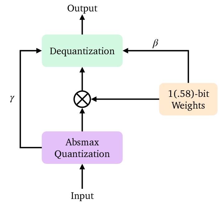
Figure 1: Illustration of the BitLinear layer.

2.2 Implementation and code availabilty

The code and data for this paper can be found on GitHub, providing readers with the resources needed to reproduce our results or adapt the BitLinear layer for their own implementations.

Currently, our implementation of BitLinear follows a pseudo-quantized approach. While weights are constrained to binary or ternary values, matrix multiplications are performed in full precision (32 or 64 bits). This is because current GPU hardware does not yet support efficient computations at such low precisions, but only to 4-bit integers in some cases [169]. However, specific computation kernels for CPUs are currently in development [170, 171]. A proper study on timing and resource consumption of BitNet is therefore not part of the present work and remains an avenue for future research. Our pseudo-quantized approach is, however, sufficient for this work, as we focus on evaluating performance metrics rather than computational efficiency.

3 Classification: Quark-gluon tagging

In this section, we employ BitNet for a quark-gluon discrimination task, utilizing the Particle Dual Attention Transformer (P-DAT) [76]. This architecture is specifically designed to capture both local particle-level information and global jet-level correlations.

To evaluate the performance of the default P-DAT and its quantized counterpart, P-DAT-Bit, we utilize the Quark-Gluon benchmark dataset [172], which consists of:

$$\begin{split}\text{Signal}:&\qquad q\bar{q}\to{\mathrm{Z}}(\to\nu\bar{\nu})+q_{uds},\\ \text{Background}:&\qquad q\bar{q}\to{\mathrm{Z}}(\to\nu\bar{\nu})+{\mathrm{g}}\;.\end{split}$$ (4)

Jet clustering is performed using the anti-$k_{T}$ algorithm with a radius parameter of $R=0.4$ using FastJet [173]. We select only jets with transverse momentum $p_{\text{T}}\in$ [500, 550] GeV and rapidity $|y|<1.7$ for further analysis. The dataset contains not only the four-momenta of each particle but also particle identification labels, including electron, muon, charged hadron, neutral hadron, and photon.

The dataset is divided into 1.6M training events, 200k validation events, and 200k test events. Our study focuses on the leading 100 constituents per jet, leveraging their four-momentum components and particle identification labels as input features for training. For jets containing fewer than 100 particles, we apply zero-padding to maintain uniform input dimensionality.

3.1 Particle Dual Attention Transformer

P-DAT takes the particle information within the jet as input and consists of three main components: (i) the feature extractor, (ii) the particle attention module, and (iii) the channel attention module. In this work, we introduce a quantized variant, P-DAT-Bit, where we apply different quantization strategies to various parts of the model.

Specifically, we employ QAT for the particle and channel attention modules while keeping other components, including the feature extractor, 1D CNN, and final multi-layer perceptron (MLP) classifier, in full precision. This is achieved by replacing all linear layers with BitLinear layers in the two particle attention and two channel attention modules, affecting approximately 63% of the total weight parameters. The attention modules incorporate physics-motivated bias terms in the scaled dot-product attention, which remain in full precision to preserve critical information. The final output undergoes a 1D CNN transformation and global average pooling before being fed into an MLP classifier. Further architectural details can be found in Ref. [76]. The new model is trained from scratch, with all hyperparameters identical to the non-quantized version.

3.2 Performance comparison

As depicted in Tab. 1, while P-DAT itself offers robust performance with an accuracy of 0.839 and an AUC of 0.9092, the adaptation of this model into P-DAT-Bit reveals both the strengths and the trade-offs of utilizing BitLinear layers within the attention blocks. The integration of BitLinear layers in P-DAT-Bit results in a slight decrease in accuracy (0.834) and AUC (0.9040) compared to its predecessor. Despite this modest drop, the performance metrics remain highly competitive, indicating that the reduced precision computation does not drastically compromise the model’s discriminative capability. Specifically, the background rejection rates at 50% signal efficiency (Rej_50%) and 30% signal efficiency (Rej_30%) are 35.0 and 83.3, respectively. This variation between P-DAT and P-DAT-Bit highlights the balancing act between computational efficiency and performance accuracy. It emphasizes that while BitLinear layers streamline model operations—particularly advantageous in resource-constrained environments—there is a nuanced impact on the model’s ability to manage complex discriminative tasks.

	Accuracy	AUC	Rej50%	Rej30%
ParticleNet [174]	0.840	0.9116	$39.8\pm 0.2$	$98.6\pm 1.3$
PCT [175]	0.841	0.9140	$43.2\pm 0.7$	$118.0\pm 2.2$
LorentzNet [176]	0.844	0.9156	$42.4\pm 0.4$	$110.2\pm 1.3$
ParT [177]	0.849	0.9203	$47.9\pm 0.5$	$129.5\pm 0.9$
P-DAT [76]	0.839	0.9092	$39.2\pm 0.6$	$95.1\pm 1.3$
P-DAT-Bit	0.834	0.9040	$35.0\pm 0.3$	$83.3\pm 1.2$

Table 1: Comparison among the performance reported for P-DAT, P-DAT-Bit, and some existing classification algorithms on the quark-gluon discrimination dataset. The uncertainties in rejection rates are calculated by taking the standard deviation of 5 training runs with different random weight initialization. The error bars for accuracy and AUC are not displayed since the variation is negligible relative to the expected values. The results for other benchmark algorithms are referred to [174, 175, 177, 176].

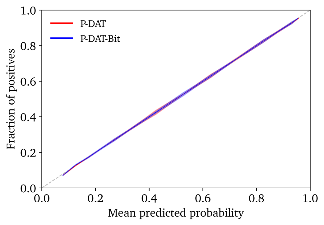
Figure 2: Calibration curves of P-DAT and P-DAT-Bit models for quark/gluon discrimination. The errorband has been obtained from evaluating 5 independent runs.

Finally, in Fig. 2, we present the calibration curves of P-DAT and P-DAT-Bit models for quark/gluon discrimination. The red line represents the calibration curve for the original P-DAT model, while the blue line represents the P-DAT-Bit model. Each model was evaluated over five runs to compute the average calibration curve and the associated standard deviation. Both models demonstrate good calibration performance, with their curves closely following the diagonal line, indicating that the predicted probabilities are well-calibrated with the actual positive class probabilities. Notably, the error bands for both models are very small, suggesting that the predictions of both models are consistent across multiple runs. Besides, the blue band of the P-DAT-Bit model is slightly broader compared to the red band of the P-DAT model, which can be attributed to its use of lower bit precision for weights and inputs in 60% of its parameters. Despite this, the P-DAT-Bit model maintains a good calibration performance, closely following the ideal diagonal line, indicating that its predicted probabilities are generally accurate.

4 Regression: SMEFT parameter estimation

In this section, we evaluate the performance of BitNet for a regression task and focus on the SMEFTNet [117] architecture. We denote its quantized version as SMEFTNet-Bit, where either all or some linear layers are replaced with its BitLinear counterpart. To perform a meaningful comparison, we employ the same simulated ${\mathrm{W}}{\mathrm{Z}}$ event samples used in Ref. [117], focusing on a semi-leptonic decay chain

$${\mathrm{p}}{\mathrm{p}}\to{\mathrm{W}}(\to q\bar{q})\,{\mathrm{Z}}(\to\ell\bar{\ell})\;.$$ (5)

The goal is to predict the decay plane angle $\phi^{\text{jet}}_{\text{decay}}$ of the parton-level quarks from the particle-level jet information, as this observable is sensitive to linear SMEFT–SM interference effects. This decay plane angle depends on the exact momenta of the up-type and down-type quarks, and interchanging these momenta at the parton level results in a difference of $\pi$. However, the particle-level decay products do not contain this information and are thus invariant under this permutation. Hence, in order to capture this ambiguity in the training of the network $f_{\theta}(x)$ with trainable parameters $\theta$, we use the modified loss function [117]

$$\mathcal{L}=\left\langle\sin^{2}\left(f_{\theta}(x_{i})-\phi^{\text{jet}}_{i,\text{decay}}\right)\right\rangle_{(x_{j},\varphi_{j})\sim\mathcal{D}_{\text{train}}}\;,$$ (6)

where the $\sin$ encodes the symmetry of shifting with $\pi$. The input $x$ consists of the lab-frame momenta of each particle in a given event $j$ parametrized as

$$x=\{p_{\text{T},1},\varphi_{1},\Delta R_{1},\cdots,p_{\text{T},N_{j}},\varphi_{N_{j}},\Delta R_{N_{j}}\}\;,$$ (7)

where $N_{j}$ denotes the number of particles in this event.

4.1 SMEFTNet architecture

SMEFTNet is an IRC-safe and rotation-equivariant graph neural network. It is designed to provide an optimal observable for small deviations from the SM and enhance SMEFT sensitivity, specifically focusing on the linear SM-SMEFT interference within SMEFT. To preserve sensitivity to the linear term, it is crucial to consider the orientation of the decay planes of the $\mathrm{W}$  or $\mathrm{Z}$  boson, as this orientation helps resolve the helicity configuration of the amplitude that is altered in the SMEFT [178]. To study the hadronic final states of $\mathrm{W}$  or $\mathrm{Z}$  boson, SMEFTNet is constructed to be equivariant to azimuthal rotations of the constituents of the boosted jet around the jet axis, maintaining SO(2) symmetry regardless of the chosen reference frame. It processes inputs as variable-length lists of particle constituents of a fat jet, originating from the hadronic decay of a boosted massive particle. For details on the architecture, we refer to Ref. [117].

In our study, we consider three quantized variants of the SMEFTNet model and apply the three variants to predict the decay plane angle from the jet’s constituents and compare their performance with the results presented in Ref [117]. In the first variant, all linear layers are replaced with BitLinear layers, which we refer to as SMEFTNet-Bit. In the second variant, only the linear layers within the MLP block are quantized, corresponding to approximately 70% of the total weight parameters; this configuration is labeled SMEFTNet-Bit70. In the third variant, only the linear layers in the Message Passing Neural Network block are quantized, accounting for about 30% of the weights; this is denoted SMEFTNet-Bit30.

4.2 Performance comparison

To visualize the comparative analysis of SMEFTNet and SMEFTNet-Bit, Fig. 3 presents the scatter plots of the true and the predicted $\varphi_{\textrm{decay}}$ in the remaining 20% ${\mathrm{W}}{\mathrm{Z}}$ dataset, respectively. The results reveal that while the SMEFTNet-Bit model marginally underperforms relative to the original SMEFTNet, the differences are minimal, showcasing the effectiveness of the low-bit model in capturing the essential structure of the data despite its limited weight and input precision. Notably, the scatter plot of SMEFTNet exhibits two faint vertical red bands at true $\phi_{\text{decay}}$ values of $\pm\pi/2$, which become more pronounced and broader in the SMEFTNet-Bit scatter plot. This phenomenon is attributed to both models’ tendency to stabilize at local minima due to the inherent challenges posed by multi-objective optimization. With two regression targets at the critical true $\phi_{\text{decay}}$ values, each model confronts conflicting optimal solutions that necessitate a compromise, potentially deviating from the global optimum for any single objective. The broader bands in the SMEFTNet-Bit results are explained by its limited precision due to weight and input quantization. This restricted precision leads to significant fluctuations in the predicted $\phi_{\text{decay}}$ values, resulting in the observed wider bands in the visual representations.

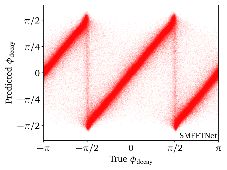
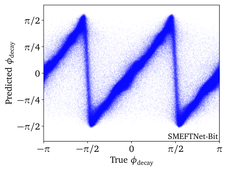
Figure 3: Two-dimensional scatter plots of the true and predicted angle $\phi_{\text{decay}}$ in the test dataset. Left: SMEFTNet with regular linear layers. Right: SMEFTNet-Bit with BitLinear layers.

Finally, Fig. 4 presents three histograms of residuals, which represent the differences between truths and predictions for $\phi_{\text{j, decay}}$. In each histogram, the red bars correspond to the original SMEFTNet, while the blue bars represent different configurations of the SMEFTNet-Bit model. In the left histogram, the blue bars correspond to SMEFTNet-Bit where all linear layers in SMEFTNet are replaced with BitNet layers. In the middle histogram, the blue bars represent the SMEFTNet-Bit70 where the linear layer weights in the MLP block are quantized, accounting for 70% of the total weight parameters. In the right histogram, the blue bars represent the SMEFTNet-Bit30 with quantized linear layer weights in the Message Passing NN block, accounting for 30% of the total weight parameters. In all cases, the SMEFTNet model exhibits a sharp peak at zero, indicating a precise alignment of predictions with true values. When fully quantized (100%), the SMEFTNet-Bit distribution broadens prominently, reflecting larger variations in prediction accuracy. Reducing the fraction of quantized layers to 70% yields intermediate performance: the residuals of SMEFTNet-Bit70 remain somewhat more dispersed than SMEFTNet but are considerably narrower than the fully quantized version. At 30% quantization, the residuals of SMEFTNet-Bit30 closely resemble those of the original SMEFTNet, showing only a modest increase in width. Consequently, it is evident that as more linear layers are replaced by BitNet layers, the performance of the model deteriorates. Moreover, a notable feature in all plots is the periodic structure of the residuals, which arises because the model faces a periodic ambiguity in which angles separated by $\pi$ map to the same predicted value, creating these peaks around $\pm\pi$ and 0 in the residual distribution. Furthermore, the fraction at $\pm\frac{\pi}{2}$ is higher for SMEFTNet-Bit, reflecting its broader vertical band in its 2D scatter plots. This broadening stems from the limited precision of BitLinear layers, which amplifies prediction fluctuations near critical values of $\pm\pi$. Notably, as the proportion of quantized layers increases, the fraction at $\pm\frac{\pi}{2}$ also becomes higher, indicating that stronger quantization further destabilizes the predictions near critical values of $\pm\pi$. By contrast, SMEFTNet shows narrower bands, indicating more accurate predictions and a lower fraction at $\pm\frac{\pi}{2}$. Lastly, across all three configurations, both models overlap around zero residuals, highlighting their overall reliability. However, the progressive widening of SMEFTNet-Bit’s distributions with increasing quantization underscores the trade-off between model compression and predictive precision—demonstrating that partial, rather than complete, quantization can give a better balance for resource-limited applications.

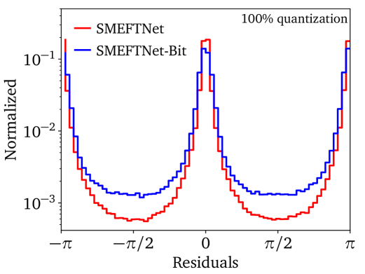
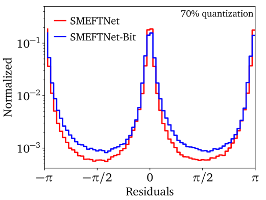
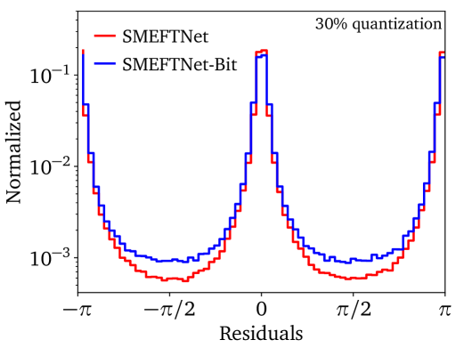
Figure 4: Histograms of residuals, defined as the differences between truths and predictions for $\phi_{\text{decay}}$ regression task. The histogram in blue represents SMEFTNet without BitLinear layers, whereas the histogram in red corresponds to SMEFTNet with BitLinear layers. From left to right: 100%, 70%, and 30% of the weights are quantized.

5 Generative: Detector simulation

Next, we consider a generative task. These are very important in HEP, as the process of sampling random events from a given (complicated) conditional probability density is precisely what happens in numerical simulations of particle collisions (See [1] for on overview on ML applications to the entire simulation chain.). One notable challenge is detector simulations, which involve modeling showers of energetic particles in the calorimeters—a task characterized by its high numerical complexity and dimensionality. In the past years, this field has seen many new ideas and approaches [179], which led to the conception of the CaloChallenge [180] to compare existing models on equal footing and spur even more development of state-of-the-art methods. The CaloChallenge was a data challenge in the HEP community, with four different datasets, increasing in their dimensionality. The goal of the challenge was to train generative networks on the datasets and to generate artificial samples as fast and precise as possible [181]. The dataset dimensionalities range from a few hundred in the easiest case to a few tens of thousands in the most complicated case. These are single particle showers, simulated with Geant4 [182, 183, 184] and available at [185, 186, 187, 188]. For more details on the datasets we refer to [180].

As an example for generative networks, we consider two well-performing submissions of the CaloChallenge [180]—CaloINN [55] based on a normalizing flow and CaloDREAM [56] based on conditional flow matching. Normalizing flows were the first generative model that passed the “classifier test” [39, 189] in calorimeter shower simulations and have seen various applications to this task [57, 55, 190, 191, 192, 48, 39, 41, 46, 180]. Conditional flow matching is the most recent generative model that was explored in this context and shows impressive performance in many applications [56, 193, 194], possibly becoming more widely used in the future.

5.1 Normalizing Flow — CaloINN

CaloINN [55] is a normalizing-flow-based generative model, learning a bijective transformation between a simple base distribution—usually a Gaussian—and a more complicated distribution—the target distribution. In detail, CaloINN is based on coupling layer-based normalizing flow [195, 196] (which are sometimes also called INN, invertible neural networks [197], even though they all are invertible). These types of flows are equally fast to evaluate in both directions (as density estimator and generative model), making training and generation more efficient than in an autoregressive setup [39, 41, 46]. The bijective transformation that is used in the coupling blocks is based on splines [198, 199, 200].

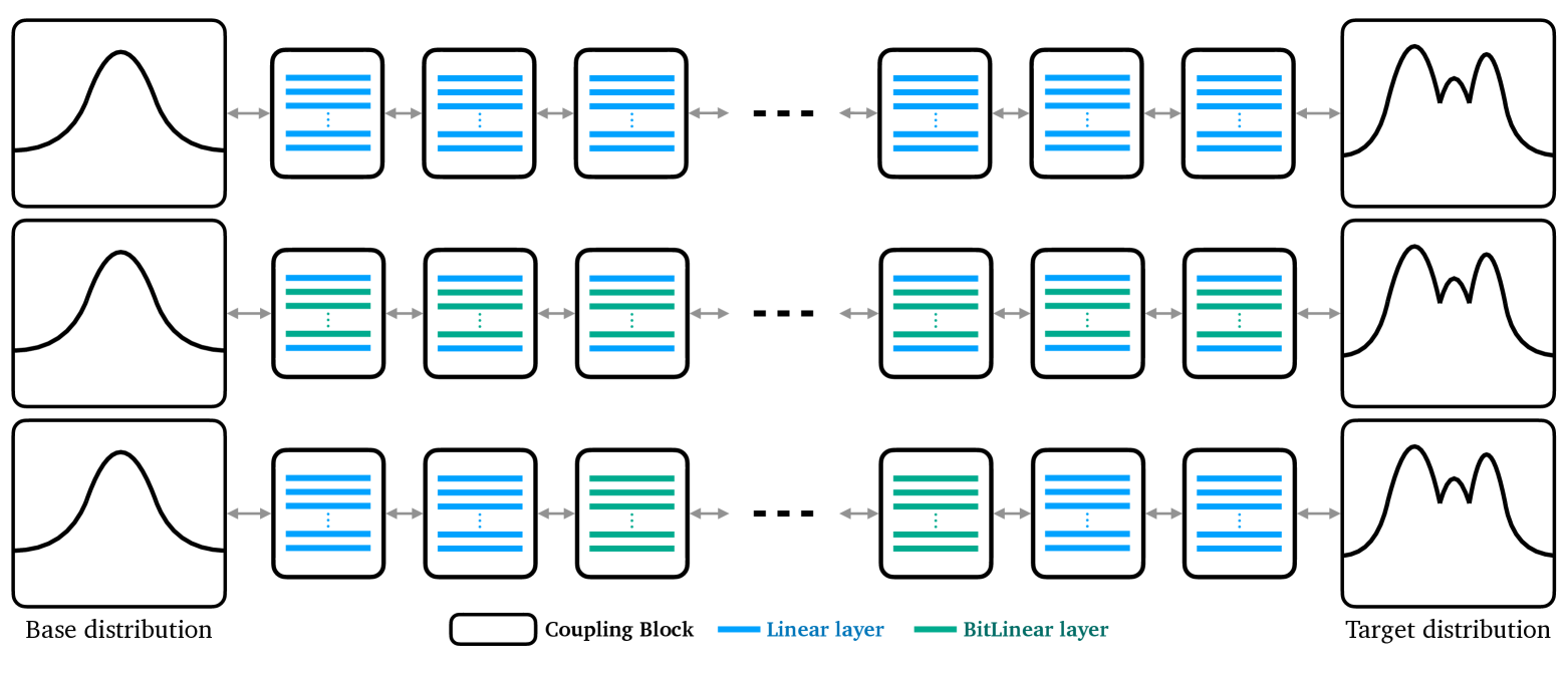
Figure 5: Illustration of different levels of quantization for the flow. Blue lines represent regular linear layers, while green lines indicate BitLinear layers. The three setups, from top to bottom, are: regular, NNCentral, and BlockCentral.

The calorimeter showers are normalized to unit energy in each calorimeter layer, and the corresponding layer energies are then appended to this array and encoded via ratios to the incident energy. This setup allows CaloINN to learn the distribution of calorimeter showers in a single step instead of a more time-consuming two-step procedure [39, 41, 46]. The downside of this approach is the scaling with the dimensionality of the dataset. The spline-based transformation requires a large number of output parameters for the individual NNs in the coupling layers, which in turn increases the number of trainable parameters of the NN. For dataset 2, CaloINN already has $270$M parameters, making an application to the six times bigger dataset 3 of the CaloChallenge impossible.

All hyperparameters are as in the original publication [55], with the flow consisting of 12 (14) coupling blocks and the individual NNs having 256 hidden nodes, and 4 (3) hidden layers for dataset 1 (2). For dataset 1, CaloINN uses rational quadratic splines [199], for dataset 2 it uses cubic splines [200]. For quantization, we consider 5 different setups, or quantization strategies, which we can summarize as follows:

Default:

The setup used in the original publication [55], without quantization. It serves as a baseline as well as a confirmation that we use the same hyperparameters as Ref. [55].

Exchange Permutation:

A setup where we change the permutations between the bijector blocks. Instead of using random permutations throughout, we exchange the sets that are transformed and that go into the NN after the first and before the last bijector. This strategy ensures that every dimension is transformed exactly once by both the first and last two bijectors. There is no quantization in this setup. It serves as a baseline for the BlockCentral setup, as it shares the same permutation scheme.

NNCentral:

Only the central layers in each NN are quantized. Since in spline-based flows the final layer typically has the most parameters, this configuration has minimal effects.

BlockCentral:

Quantization is applied to all layers of NNs in the central bijectors, i.e. neither the first two nor the last two in the chain. Paired with the same permutation strategy as in Exchange Permutation, this ensures each dimension is first transformed by a regular bijector, then by quantized ones, and finally again by a regular bijector.

All:

All linear layers in all bijectors are quantized.

Fig. 5 shows an illustration of the regular, NNCentral and BlockCentral. Their fractions of quantized weights are given in Tab. 2. To evaluate the performance of the quantized CaloINN, we use the exactly same classifier architecture and training strategy as in [180], making the results directly comparable. The main results are shown in Tab. 2.

Dataset	Setup		Quantization	Low-Level AUC	High-Level AUC
ds1–$\gamma$	reg.	Default	-	0.633(3)	0.656(3)
		Exchange Perm.	-	0.640(4)	0.651(3)
	quant.	NNCentral	$8.4$%	0.640(3)	0.650(2)
		BlockCentral	$66.6$%	0.680(3)	0.669(3)
		All	$99.9$%	0.759(2)	0.828(2)
ds1–$\pi^{+}$	reg.	Default	-	0.793(3)	0.742(3)
		Exchange Perm.	-	0.784(2)	0.736(3)
	quant.	NNCentral	$5.9$%	0.801(2)	0.751(3)
		BlockCentral	$66.6$%	0.852(1)	0.807(2)
		All	$99.9$%	0.882(2)	0.907(2)
ds2	reg.	Default	-	0.738(4)	0.859(2)
		Exchange Perm.	-	0.728(6)	0.857(3)
	quant.	NNCentral	$0.3$%	0.780(3)	0.876(4)
		BlockCentral	$71.4$%	0.950(2)	0.979(1)
		All	$99.9$%	0.993(1)	0.998(0)

Table 2: Performance of default and BitNet CaloINN using the classifier metric of the CaloChallenge [180]. Uncertainties show the standard deviation over 10 random initializations and trainings of the classifier on the same CaloINN sample.

The AUCs we see in the regular setup are consistent with the ones reported in [180], where ds1 photon was scored 0.626(4) / 0.638(3), ds1 pion was scored 0.784(2) / 0.732(2), and ds2 was scored 0.743(2) / 0.865(3) for low / high-level observables, respectively. These AUCs differ from the ones presented in [55] as the classifier architecture in the original publication was different than the one used here and in [180]. The modified permutations usually improve the AUCs slightly, but mostly they agree with the regular setup within one standard deviation.

We observe that quantizing the NN weights with the BitNet degrades performance, with a clear correlation between the fraction of quantization and the AUC. Across all datasets, the NNCentral setup gives AUCs almost as good as the Regular setup, but in this case only a very low fraction of weights is actually quantized. The All setup degrades the generative performance a lot, with the gap being larger in the high-dimensional dataset 2. The BlockCentral setup results in an overall good performance. This is an interplay of not having quantized all of the parameters and the choice to only quantize the central coupling layers instead of the outer ones. This latter choice allows for the bulk of the bijection being carried out by a quantized flow, while the final details will be adjusted in the outer coupling blocks with a regular flow setup.

5.2 Conditional Flow Matching — CaloDREAM

CaloDREAM [56] is a generative architecture combining Conditional Flow Matching (CFM) with transformer elements.

In detail, CaloDREAM consists of two networks, both trained with conditional flow matching: (i) an autoregressive transformer, called the energy network, to learn the 45 layer energies, and (ii) a vision transformer, called the shape network, learning the normalized showers. The self-attention mechanism in the transformer layers is highly beneficial for modeling the sparsity of calorimeter showers and the correlations across detector locations. Crucially, the introduction of patching—which groups nearby voxels into coarser units—reduces the impact of the quadratic scaling and enables the model to scale efficiently to larger calorimeter geometries such as DS3. At the same time, conditional flow matching ensures efficient training of the underlying continuous normalizing flow model.

The main difference of CaloDREAM to CaloINN when considering the quantization lies in the distribution of NNs in the generative process: instead of many “smaller” NNs in CaloINN, CaloDREAM has one large NN for each of the two steps, so we expect the impact of quantization on performance to be smaller.

The preprocessing of the calorimeter shower data is done as in the CaloINN setup. Showers are normalized per calorimeter layer, and the corresponding layer energies are encoded as ratios to constrain them to the range $\left[0,1\right]$. The energy network now learns the latter independently from the normalized showers, which are learned by the shape network.

Since the two networks factorize, we can discuss quantization strategies separately and combine them ad libitum in generation.

Quantization of the energy network

In the energy network, an autoregressive transformer defines the embeddings of the energy values that are then passed to a MLP performing the CFM. We keep the original hyperparameter choices for these networks, so the former is based on 4 attention heads with an embedding dimension of 64, see [56]. The feed-forward CFM network consists of 8 hidden layers with 256 nodes each. It takes the concatenated 64-dimensional time embedding, the 64-dimensional autoregressive embedding of previous calorimeter layer energies as well as the 1-dimensional current calorimeter layer energy as input and predicts the velocity field of the current calorimeter layer as output. We consider two quantization setups for the energy network:

Regular:

The non-quantized version, as used in the original publication [56].

Quantized:

Quantizes the central 6 of the 8 hidden layers of the CFM network, leaving the transformer-based embedding networks untouched. This results in 66.09% of the trainable parameters of the energy network being quantized. However, since the energy network is much smaller than the shape network, this translates to only 5.54% of the total CaloDREAM model being quantized.

Quantization of the shape network

In the shape network, all 6480 voxels of the calorimeter are split into 135 patches of 48 voxels each, and all operations are performed on these patches in parallel. Diffusion time $t$, ratios of layer energies, incident energy, and voxel patches are transformed using three different embedding networks: (i) for time, (ii) for conditionals, and (iii) for position. These embeddings are passed to a chain of 6 Vision Transformer (ViT) blocks, each consisting of a self-attention layer, a projection, and a subsequent MLP step. The output is then passed through a final MLP layer and reassembled from patches into complete calorimeter showers.

Given the modular nature of the shape network, several quantization strategies are possible. Here, we report three:

Regular:

The non-quantized version, identical to the setup in the original publication [56].

No embedding:

Quantizes the core elements of the ViT blocks—QKV matrices, projections, and MLPs—while keeping the embedding networks and the final MLP layer unquantized. This configuration results in 63.8% of the shape network being quantized.

Full:

Extends the no embedding setup by also quantizing the linear layers in the position, time, and conditional embedding networks. This increases the fraction of quantized parameters in the shape network to 66.22%.

Performance comparison

Also for the evaluation of CaloDREAM, we use the same classifier architecture and training strategy as in the CaloChallenge [180], making the results directly comparable. The main results are shown in Tab. 3.

Energy net	Shape net	Quantization	low-level AUC	high-level AUC
regular	regular	-	0.531(3)	0.523(3)
quantized		$5.5$%	0.532(3)	0.525(3)
regular	no embedding	$58.5$%	0.611(2)	0.543(3)
quantized		$63.9$%	0.610(5)	0.545(2)
regular	full	$60.7$%	0.735(4)	0.942(2)
quantized		$66.2$%	0.738(4)	0.944(3)

Table 3: Performance of regular and BitNet CaloDREAM using the classifier metric of the CaloChallenge [180]. Uncertainties show the standard deviation over 10 random initializations and trainings of the classifier on the same CaloDREAM sample.

Our retraining of CaloDREAM in the regular setup reproduces the scores of the CaloChallenge [180] with 0.531(3) / 0.521(2) for low/high-level AUC.

The first thing we observe in Tab. 3 is that swapping the regular for the quantized energy network has no effect on the resulting AUC scores, so 66% of trainable parameters in six out of eight hidden layers inside the CFM can safely be quantized without loss of sample quality.

In the shape network, however, the performance strongly depends on which parts are quantized. A substantial part of the ViT blocks can be quantized with almost no loss in shower quality, but as soon as the embedding layers are quantized, the performance drops a lot. Note that the no embedding CaloDREAM, which is quantized to about 60% still has the best high-level, and second best low-level AUCs of the CaloChallenge submissions [180].

We also observe the spread between high- and low-level AUC to be larger. Especially in the fully quantized case, the high-level features were already very sensitive. The low-level AUC score was not as bad, but that is likely a remnant of the classifier architecture choice, see the discussion in [180].

6 Conclusions and Outlook

In this paper, we investigated the applicability of the BitNet architecture to various tasks in high-energy physics. We demonstrated that QAT can offer a promising path forward for large-scale neural network applications in HEP. By applying these techniques to classification, regression, and generative tasks, we observed that performance remains competitive, especially for classification tasks such as quark–gluon tagging. However, the impact of quantization on regression and generative modeling is more nuanced and requires careful consideration of network size and architecture. The results highlight that:

• Larger networks can be quantized more easily. Our experiments with different generative architectures used in detector simulation—specifically the normalizing flow-based CaloINN and the flow matching-based CaloDREAM — indicate that larger models often exhibit smoother quantization behavior. For instance, with around 66% of its parameters quantized, CaloINN experiences a noticeable drop in sample quality, whereas CaloDREAM, which also quantizes roughly 63.8% of its shape network, exhibits only minor performance degradation. These observations underscore how larger networks provide greater representational capacity, making them more resilient to the information loss introduced by low-bit representations. Consequently, these results highlight the potential of quantized, large-scale generative models in tackling the complex, high-dimensional tasks typical of modern particle physics experiments.

• Performance depends on the layer chosen for quantization. In our generative studies for detector simulation, CaloINN benefits from selectively quantizing all layers within the central bijectors (BlockCentral), thereby maintaining decent sample quality even at about 66% quantized weights, while fully quantizing all layers (99.9%) severely degrades performance. Likewise, in CaloDREAM, quantizing the elements within the shape network’s ViT blocks (QKV matrices, projections, and MLPs) results in minimal performance loss; however, once the embedding layers are quantized, performance drops considerably. These findings underscore how carefully selecting which sections of the network to quantize—central layers versus outer layers, embedding networks versus projection layers—can preserve model fidelity and better adapt to each architecture’s demands, especially for high-dimensional tasks in particle physics. Further studies in automatic, heterogeneous quantization [201, 202] are needed to fully extract the best performance of the networks.

• Quantizing more layers generally degrades model performance. Our SMEFTNet experiments demonstrate that as the proportion of quantized layers increases, the precision of the predictions decreases. The fully quantized SMEFTNet-Bit shows the largest degradation, while selectively quantizing only 30% of the linear layers (within the message-passing block) leads to a minimal drop in performance. These results highlight the trade-off between model compression and accuracy, emphasizing the need for selective quantization to balance efficiency and precision.

• Certain layers are robust to quantization. Self-attention layers in transformer-based models, such as P-DAT or the shape network ViT in CaloDREAM, exhibit surprisingly minimal performance degradation thanks to their ability to encode attention patterns effectively with discrete weights. This finding points to the potential of applying low-bit quantization in attention-driven architectures, enabling significant memory and computational savings.

• Low-bit quantization aligns with future hardware and energy constraints. As the HL-LHC generates increasingly large datasets which require more sophisticated analyses and simulations, achieving high performance while keeping the energy demands reasonable will be crucial. The low-bit QAT explored here aligns well with emerging hardware trends, where dedicated architectures for quantized operations are expected to play a central role.

The relevance of such quantization techniques is expected to grow as networks become larger and more prevalent throughout HEP workflows. Future research directions include exploring alternative weight quantization configurations, integrating these methods seamlessly into existing large-scale ML models, and adapting BitNet for high-energy physics applications through fully quantized implementations with low-precision operations, enabling a quantitative evaluation of energy, memory, and latency reductions. Moreover, extending the scope to tasks requiring real-time or near-real-time performance will further validate the robustness of quantized models under realistic experimental conditions. A typical example is the LHC trigger system, which demands extremely fast classification on resource-limited hardware such as FPGAs. While quantization techniques have been successfully applied in this context for many years, our study highlights the potential of QAT to push these approaches further, beyond the trigger. By incorporating QAT, it may become feasible to implement larger and more expressive models on FPGAs or other hardware, potentially leading to more energy-efficient, scalable, yet accurate ML applications in HEP.

References

- [1] S. Badger et al., Machine Learning and LHC Event Generation, SciPost Phys. 14 (3, 2022) 079, arXiv:2203.07460 [hep-ph].
- [2] T. Plehn, A. Butter, B. Dillon, and C. Krause, Modern Machine Learning for LHC Physicists, arXiv:2211.01421 [hep-ph].
- [3] F. Bishara and M. Montull, (Machine) Learning Amplitudes for Faster Event Generation, Phys.Rev.D 107 (12, 2019) L071901, arXiv:1912.11055 [hep-ph].
- [4] S. Badger and J. Bullock, Using neural networks for efficient evaluation of high multiplicity scattering amplitudes, JHEP 06 (2020) 114, arXiv:2002.07516 [hep-ph].
- [5] J. Aylett-Bullock, S. Badger, and R. Moodie, Optimising simulations for diphoton production at hadron colliders using amplitude neural networks, JHEP 08 (6, 2021) 066, arXiv:2106.09474 [hep-ph].
- [6] D. Maître and H. Truong, A factorisation-aware Matrix element emulator, JHEP 11 (7, 2021) 066, arXiv:2107.06625 [hep-ph].
- [7] R. Winterhalder, V. Magerya, E. Villa, S. P. Jones, M. Kerner, A. Butter, G. Heinrich, and T. Plehn, Targeting Multi-Loop Integrals with Neural Networks, SciPost Phys. 12 (2022) 129, arXiv:2112.09145 [hep-ph].
- [8] S. Badger, A. Butter, M. Luchmann, S. Pitz, and T. Plehn, Loop Amplitudes from Precision Networks, SciPost Phys. Core 6 (2023) 034, arXiv:2206.14831 [hep-ph].
- [9] D. Maître and H. Truong, One-loop matrix element emulation with factorisation awareness, arXiv:2302.04005 [hep-ph].
- [10] H. Bahl, N. Elmer, L. Favaro, M. Haußmann, T. Plehn, and R. Winterhalder, Accurate Surrogate Amplitudes with Calibrated Uncertainties, arXiv:2412.12069 [hep-ph].
- [11] J. Bendavid, Efficient Monte Carlo Integration Using Boosted Decision Trees and Generative Deep Neural Networks, arXiv:1707.00028 [hep-ph].
- [12] M. D. Klimek and M. Perelstein, Neural Network-Based Approach to Phase Space Integration, arXiv:1810.11509 [hep-ph].
- [13] I.-K. Chen, M. D. Klimek, and M. Perelstein, Improved Neural Network Monte Carlo Simulation, arXiv:2009.07819 [hep-ph].
- [14] C. Gao, J. Isaacson, and C. Krause, i-flow: High-Dimensional Integration and Sampling with Normalizing Flows, arXiv:2001.05486 [physics.comp-ph].
- [15] E. Bothmann, T. Janßen, M. Knobbe, T. Schmale, and S. Schumann, Exploring phase space with Neural Importance Sampling, arXiv:2001.05478 [hep-ph].
- [16] C. Gao, S. Höche, J. Isaacson, C. Krause, and H. Schulz, Event Generation with Normalizing Flows, Phys. Rev. D 101 (2020) 7, 076002, arXiv:2001.10028 [hep-ph].
- [17] K. Danziger, T. Janßen, S. Schumann, and F. Siegert, Accelerating Monte Carlo event generation – rejection sampling using neural network event-weight estimates, SciPost Phys. 12 (9, 2021) 164, arXiv:2109.11964 [hep-ph].
- [18] T. Heimel, R. Winterhalder, A. Butter, J. Isaacson, C. Krause, F. Maltoni, O. Mattelaer, and T. Plehn, MadNIS – Neural Multi-Channel Importance Sampling, SciPost Phys. 15 (12, 2022) 141, arXiv:2212.06172 [hep-ph].
- [19] T. Janßen, D. Maître, S. Schumann, F. Siegert, and H. Truong, Unweighting multijet event generation using factorisation-aware neural networks, SciPost Phys. 15 (1, 2023) 107, arXiv:2301.13562 [hep-ph].
- [20] E. Bothmann, T. Childers, W. Giele, F. Herren, S. Hoeche, J. Isaacsson, M. Knobbe, and R. Wang, Efficient phase-space generation for hadron collider event simulation, SciPost Phys. 15 (2023) 169, arXiv:2302.10449 [hep-ph].
- [21] N. Deutschmann and N. Götz, Accelerating HEP simulations with Neural Importance Sampling, JHEP 03 (2024) 083, arXiv:2401.09069 [hep-ph].
- [22] T. Heimel, O. Mattelaer, T. Plehn, and R. Winterhalder, Differentiable MadNIS-Lite, SciPost Phys. 18 (8, 2024) 017, arXiv:2408.01486 [hep-ph].
- [23] L. de Oliveira, M. Paganini, and B. Nachman, Learning Particle Physics by Example: Location-Aware Generative Adversarial Networks for Physics Synthesis, arXiv:1701.05927 [stat.ML].
- [24] A. Andreassen, I. Feige, C. Frye, and M. D. Schwartz, JUNIPR: a Framework for Unsupervised Machine Learning in Particle Physics, Eur.Phys.J.C 79 (2018) 102, arXiv:1804.09720 [hep-ph].
- [25] E. Bothmann and L. Debbio, Reweighting a parton shower using a neural network: the final-state case, JHEP 01 (2019) 033, arXiv:1808.07802 [hep-ph].
- [26] K. Dohi, Variational Autoencoders for Jet Simulation, arXiv:2009.04842 [hep-ph].
- [27] E. Buhmann, G. Kasieczka, and J. Thaler, EPiC-GAN: Equivariant Point Cloud Generation for Particle Jets, SciPost Phys. 15 (1, 2023) 130, arXiv:2301.08128 [hep-ph].
- [28] M. Leigh, D. Sengupta, G. Quétant, J. A. Raine, K. Zoch, and T. Golling, PC-JeDi: Diffusion for Particle Cloud Generation in High Energy Physics, SciPost Phys. 16 (3, 2023) 018, arXiv:2303.05376 [hep-ph].
- [29] V. Mikuni, B. Nachman, and M. Pettee, Fast Point Cloud Generation with Diffusion Models in High Energy Physics, Phys.Rev.D 108 (4, 2023) 036025, arXiv:2304.01266 [hep-ph].
- [30] E. Buhmann, C. Ewen, D. A. Faroughy, T. Golling, G. Kasieczka, M. Leigh, G. Quétant, J. A. Raine, D. Sengupta, and D. Shih, EPiC-ly Fast Particle Cloud Generation with Flow-Matching and Diffusion, arXiv:2310.00049 [hep-ph].
- [31] M. Paganini, L. de Oliveira, and B. Nachman, Accelerating Science with Generative Adversarial Networks: An Application to 3D Particle Showers in Multilayer Calorimeters, Phys. Rev. Lett. 120 (2018) 4, 042003, arXiv:1705.02355 [hep-ex].
- [32] L. de Oliveira, M. Paganini, and B. Nachman, Controlling Physical Attributes in GAN-Accelerated Simulation of Electromagnetic Calorimeters, J. Phys. Conf. Ser. 1085 (2018) 4, 042017, arXiv:1711.08813 [hep-ex].
- [33] M. Paganini, L. de Oliveira, and B. Nachman, CaloGAN : Simulating 3D high energy particle showers in multilayer electromagnetic calorimeters with generative adversarial networks, Phys. Rev. D97 (2018) 1, 014021, arXiv:1712.10321 [hep-ex].
- [34] M. Erdmann, L. Geiger, J. Glombitza, and D. Schmidt, Generating and refining particle detector simulations using the Wasserstein distance in adversarial networks, Comput. Softw. Big Sci. 2 (2018) 1, 4, arXiv:1802.03325 [astro-ph.IM].
- [35] M. Erdmann, J. Glombitza, and T. Quast, Precise simulation of electromagnetic calorimeter showers using a Wasserstein Generative Adversarial Network, Comput. Softw. Big Sci. 3 (2019) 1, 4, arXiv:1807.01954 [physics.ins-det].
- [36] D. Belayneh et al., Calorimetry with Deep Learning: Particle Simulation and Reconstruction for Collider Physics, arXiv:1912.06794 [physics.ins-det].
- [37] E. Buhmann, S. Diefenbacher, E. Eren, F. Gaede, G. Kasieczka, A. Korol, and K. Krüger, Getting High: High Fidelity Simulation of High Granularity Calorimeters with High Speed, Comput. Softw. Big Sci. 5 (2021) 1, 13, arXiv:2005.05334 [physics.ins-det].
- [38] E. Buhmann, S. Diefenbacher, E. Eren, F. Gaede, G. Kasieczka, A. Korol, and K. Krüger, Decoding Photons: Physics in the Latent Space of a BIB-AE Generative Network, EPJ Web Conf. 251 (2, 2021) 03003, arXiv:2102.12491 [physics.ins-det].
- [39] C. Krause and D. Shih, CaloFlow: Fast and Accurate Generation of Calorimeter Showers with Normalizing Flows, Phys.Rev.D 107 (6, 2021) 113003, arXiv:2106.05285 [physics.ins-det].
- [40] ATLAS Collaboration, AtlFast3: the next generation of fast simulation in ATLAS, Comput. Softw. Big Sci. 6 (2022) 7, arXiv:2109.02551 [hep-ex].
- [41] C. Krause and D. Shih, CaloFlow II: Even Faster and Still Accurate Generation of Calorimeter Showers with Normalizing Flows, Phys.Rev.D 107 (10, 2021) 113004, arXiv:2110.11377 [physics.ins-det].
- [42] E. Buhmann, S. Diefenbacher, E. Eren, F. Gaede, D. Hundhausen, G. Kasieczka, W. Korcari, K. Krüger, P. McKeown, and L. Rustige, Hadrons, Better, Faster, Stronger, Mach.Learn.Sci.Tech. 3 (12, 2021) 025014, arXiv:2112.09709 [physics.ins-det].
- [43] C. Chen, O. Cerri, T. Q. Nguyen, J. R. Vlimant, and M. Pierini, Analysis-Specific Fast Simulation at the LHC with Deep Learning, Comput. Softw. Big Sci. 5 (2021) 1, 15.
- [44] V. Mikuni and B. Nachman, Score-based Generative Models for Calorimeter Shower Simulation, Phys.Rev.D 106 (6, 2022) 092009, arXiv:2206.11898 [hep-ph].
- [45] ATLAS Collaboration, Deep generative models for fast photon shower simulation in ATLAS, Comput.Softw.Big Sci. 8 (10, 2022) 7, arXiv:2210.06204 [hep-ex].
- [46] C. Krause, I. Pang, and D. Shih, CaloFlow for CaloChallenge Dataset 1, SciPost Phys. 16 (10, 2022) 126, arXiv:2210.14245 [physics.ins-det].
- [47] J. C. Cresswell, B. L. Ross, G. Loaiza-Ganem, H. Reyes-Gonzalez, M. Letizia, and A. L. Caterini, CaloMan: Fast generation of calorimeter showers with density estimation on learned manifolds, in 36th Conference on Neural Information Processing Systems. 11, 2022. arXiv:2211.15380 [hep-ph].
- [48] S. Diefenbacher, E. Eren, F. Gaede, G. Kasieczka, C. Krause, I. Shekhzadeh, and D. Shih, L2LFlows: Generating High-Fidelity 3D Calorimeter Images, JINST 18 (2, 2023) P10017, arXiv:2302.11594 [physics.ins-det].
- [49] H. Hashemi, N. Hartmann, S. Sharifzadeh, J. Kahn, and T. Kuhr, Ultra-High-Resolution Detector Simulation with Intra-Event Aware GAN and Self-Supervised Relational Reasoning, Nature Commun. 15 (3, 2023) 4916, arXiv:2303.08046 [physics.ins-det].
- [50] A. Xu, S. Han, X. Ju, and H. Wang, Generative Machine Learning for Detector Response Modeling with a Conditional Normalizing Flow, JINST 19 (3, 2023) P02003, arXiv:2303.10148 [hep-ex].
- [51] S. Diefenbacher, E. Eren, F. Gaede, G. Kasieczka, A. Korol, K. Krüger, P. McKeown, and L. Rustige, New Angles on Fast Calorimeter Shower Simulation, Mach.Learn.Sci.Tech. 4 (3, 2023) 035044, arXiv:2303.18150 [physics.ins-det].
- [52] E. Buhmann, S. Diefenbacher, E. Eren, F. Gaede, G. Kasieczka, A. Korol, W. Korcari, K. Krüger, and P. McKeown, CaloClouds: Fast Geometry-Independent Highly-Granular Calorimeter Simulation, JINST 18 (5, 2023) P11025, arXiv:2305.04847 [physics.ins-det].
- [53] M. R. Buckley, C. Krause, I. Pang, and D. Shih, Inductive simulation of calorimeter showers with normalizing flows, Phys. Rev. D 109 (2024) 3, 033006, arXiv:2305.11934 [physics.ins-det].
- [54] S. Diefenbacher, V. Mikuni, and B. Nachman, Refining Fast Calorimeter Simulations with a Schrödinger Bridge, arXiv:2308.12339 [physics.ins-det].
- [55] F. Ernst, L. Favaro, C. Krause, T. Plehn, and D. Shih, Normalizing Flows for High-Dimensional Detector Simulations, arXiv:2312.09290 [hep-ph].
- [56] L. Favaro, A. Ore, S. P. Schweitzer, and T. Plehn, CaloDREAM – Detector Response Emulation via Attentive flow Matching, arXiv:2405.09629 [hep-ph].
- [57] T. Buss, F. Gaede, G. Kasieczka, C. Krause, and D. Shih, Convolutional L2LFlows: Generating Accurate Showers in Highly Granular Calorimeters Using Convolutional Normalizing Flows, JINST 19 (5, 2024) P09003, arXiv:2405.20407 [physics.ins-det].
- [58] G. Quétant, J. A. Raine, M. Leigh, D. Sengupta, and T. Golling, PIPPIN: Generating variable length full events from partons, Phys.Rev.D 110 (6, 2024) 076023, arXiv:2406.13074 [hep-ph].
- [59] ATLAS Collaboration, Quark versus Gluon Jet Tagging Using Jet Images with the ATLAS Detector, tech. rep., CERN, Geneva, Jul, 2017.
- [60] P. T. Komiske, E. M. Metodiev, and M. D. Schwartz, Deep learning in color: towards automated quark/gluon jet discrimination, JHEP 01 (2017) 110, arXiv:1612.01551 [hep-ph].
- [61] T. Cheng, Recursive Neural Networks in Quark/Gluon Tagging, arXiv:1711.02633 [hep-ph].
- [62] M. Stoye, J. Kieseler, M. Verzetti, H. Qu, L. Gouskos, A. Stakia, and CMS Collaboration, DeepJet: Generic physics object based jet multiclass classification for LHC experiments, Proceedings of the Deep Learning for Physical Sciences Workshop at NIPS (2017) (2017) , in Proceedings of the Deep Learning for Physical Sciences Workshop at NIPS (2017). 2017.
- [63] Y.-T. Chien and R. Kunnawalkam Elayavalli, Probing heavy ion collisions using quark and gluon jet substructure, arXiv:1803.03589 [hep-ph].
- [64] E. A. Moreno, O. Cerri, J. M. Duarte, H. B. Newman, T. Q. Nguyen, A. Periwal, M. Pierini, A. Serikova, M. Spiropulu, and J.-R. Vlimant, JEDI-net: a jet identification algorithm based on interaction networks, Eur. Phys. J. C 80 (2020) 1, 58, arXiv:1908.05318 [hep-ex].
- [65] G. Kasieczka, N. Kiefer, T. Plehn, and J. M. Thompson, Quark-Gluon Tagging: Machine Learning vs Detector, SciPost Phys. 6 (2019) 6, 069, arXiv:1812.09223 [hep-ph].
- [66] G. Kasieczka, S. Marzani, G. Soyez, and G. Stagnitto, Towards Machine Learning Analytics for Jet Substructure, arXiv:2007.04319 [hep-ph].
- [67] J. S. H. Lee, S. M. Lee, Y. Lee, I. Park, I. J. Watson, and S. Yang, Quark Gluon Jet Discrimination with Weakly Supervised Learning, J. Korean Phys. Soc. 75 (2019) 9, 652, arXiv:2012.02540 [hep-ph].
- [68] J. S. H. Lee, I. Park, I. J. Watson, and S. Yang, Quark-Gluon Jet Discrimination Using Convolutional Neural Networks, J. Korean Phys. Soc. 74 (2019) 3, 219, arXiv:2012.02531 [hep-ex].
- [69] F. A. Dreyer and H. Qu, Jet tagging in the Lund plane with graph networks, arXiv:2012.08526 [hep-ph].
- [70] A. Romero, D. Whiteson, M. Fenton, J. Collado, and P. Baldi, Safety of Quark/Gluon Jet Classification, arXiv:2103.09103 [hep-ph].
- [71] J. Filipek, S.-C. Hsu, J. Kruper, K. Mohan, and B. Nachman, Identifying the Quantum Properties of Hadronic Resonances using Machine Learning, arXiv:2105.04582 [hep-ph].
- [72] F. Dreyer, G. Soyez, and A. Takacs, Quarks and gluons in the Lund plane, JHEP 08 (12, 2021) 177, arXiv:2112.09140 [hep-ph].
- [73] S. Bright-Thonney, I. Moult, B. Nachman, and S. Prestel, Systematic Quark/Gluon Identification with Ratios of Likelihoods, JHEP 12 (7, 2022) 021, arXiv:2207.12411 [hep-ph].
- [74] M. Crispim Romão, J. G. Milhano, and M. van Leeuwen, Jet substructure observables for jet quenching in Quark Gluon Plasma: a Machine Learning driven analysis, SciPost Phys. 16 (4, 2023) 015, arXiv:2304.07196 [hep-ph].
- [75] D. Athanasakos, A. J. Larkoski, J. Mulligan, M. Ploskon, and F. Ringer, Is infrared-collinear safe information all you need for jet classification?, JHEP 07 (5, 2023) 257, arXiv:2305.08979 [hep-ph].
- [76] M. He and D. Wang, Quark/Gluon Discrimination and Top Tagging with Dual Attention Transformer, Eur.Phys.J.C 83 (7, 2023) 1116, arXiv:2307.04723 [hep-ph].
- [77] W. Shen, D. Wang, and J. M. Yang, Hierarchical High-Point Energy Flow Network for Jet Tagging, JHEP 09 (8, 2023) 135, arXiv:2308.08300 [hep-ph].
- [78] M. J. Dolan, J. Gargalionis, and A. Ore, Quark-versus-gluon tagging in CMS Open Data with CWoLa and TopicFlow, arXiv:2312.03434 [hep-ph].
- [79] F. Blekman, F. Canelli, A. De Moor, K. Gautam, A. Ilg, A. Macchiolo, and E. Ploerer, Jet Flavour Tagging at FCC-ee with a Transformer-based Neural Network: DeepJetTransformer, Eur.Phys.J.C 85 (6, 2024) 165, arXiv:2406.08590 [hep-ex].
- [80] J. O. Sandoval, V. Manian, and S. Malik, A multicategory jet image classification framework using deep neural network, arXiv:2407.03524 [hep-ph].
- [81] Y. Wu, K. Wang, and J. Zhu, Jet Tagging with More-Interaction Particle Transformer, arXiv:2407.08682 [hep-ph].
- [82] R. Tagami, T. Suehara, and M. Ishino, Application of Particle Transformer to quark flavor tagging in the ILC project, EPJ Web Conf. 315 (10, 2024) 03011, arXiv:2410.11322 [hep-ex].
- [83] J. Brehmer, V. Bresó, P. de Haan, T. Plehn, H. Qu, J. Spinner, and J. Thaler, A Lorentz-Equivariant Transformer for All of the LHC, arXiv:2411.00446 [hep-ph].
- [84] J. Geuskens, N. Gite, M. Krämer, V. Mikuni, A. Mück, B. Nachman, and H. Reyes-González, The Fundamental Limit of Jet Tagging, 11, 2024. arXiv:2411.02628 [hep-ph].
- [85] A. Andreassen and B. Nachman, Neural Networks for Full Phase-space Reweighting and Parameter Tuning, Phys. Rev. D 101 (2020) 9, 091901, arXiv:1907.08209 [hep-ph].
- [86] M. Stoye, J. Brehmer, G. Louppe, J. Pavez, and K. Cranmer, Likelihood-free inference with an improved cross-entropy estimator, arXiv:1808.00973 [stat.ML].
- [87] J. Hollingsworth and D. Whiteson, Resonance Searches with Machine Learned Likelihood Ratios, arXiv:2002.04699 [hep-ph].
- [88] J. Brehmer, K. Cranmer, G. Louppe, and J. Pavez, Constraining Effective Field Theories with Machine Learning, arXiv:1805.00013 [hep-ph].
- [89] J. Brehmer, K. Cranmer, G. Louppe, and J. Pavez, A Guide to Constraining Effective Field Theories with Machine Learning, arXiv:1805.00020 [hep-ph].
- [90] J. Brehmer, F. Kling, I. Espejo, and K. Cranmer, MadMiner: Machine learning-based inference for particle physics, Comput. Softw. Big Sci. 4 (2020) 1, 3, arXiv:1907.10621 [hep-ph].
- [91] J. Brehmer, G. Louppe, J. Pavez, and K. Cranmer, Mining gold from implicit models to improve likelihood-free inference, Proc. Nat. Acad. Sci. (2020) 201915980, arXiv:1805.12244 [stat.ML].
- [92] K. Cranmer, J. Pavez, and G. Louppe, Approximating Likelihood Ratios with Calibrated Discriminative Classifiers, arXiv:1506.02169 [stat.AP].
- [93] A. Andreassen, S.-C. Hsu, B. Nachman, N. Suaysom, and A. Suresh, Parameter Estimation using Neural Networks in the Presence of Detector Effects, Phys. Rev. D 103 (2021) 036001, arXiv:2010.03569 [hep-ph].
- [94] A. Coogan, K. Karchev, and C. Weniger, Targeted Likelihood-Free Inference of Dark Matter Substructure in Strongly-Lensed Galaxies, 34th Conference on Neural Information Processing Systems (10, 2020) , arXiv:2010.07032 [astro-ph.CO].
- [95] F. Flesher, K. Fraser, C. Hutchison, B. Ostdiek, and M. D. Schwartz, Parameter Inference from Event Ensembles and the Top-Quark Mass, JHEP 09 (11, 2020) 058, arXiv:2011.04666 [hep-ph].
- [96] S. Bieringer, A. Butter, T. Heimel, S. Höche, U. Köthe, T. Plehn, and S. T. Radev, Measuring QCD Splittings with Invertible Networks, SciPost Phys. 10 (12, 2020) 126, arXiv:2012.09873 [hep-ph].
- [97] B. Nachman and J. Thaler, E Pluribus Unum Ex Machina: Learning from Many Collider Events at Once, Phys.Rev.D 103 (1, 2021) 116013, arXiv:2101.07263 [physics.data-an].
- [98] S. Chatterjee, N. Frohner, L. Lechner, R. Schöfbeck, and D. Schwarz, Tree boosting for learning EFT parameters, Comput.Phys.Commun. 277 (7, 2021) 108385, arXiv:2107.10859 [hep-ph].
- [99] S. Shirobokov, V. Belavin, M. Kagan, A. Ustyuzhanin, and A. G. Baydin, Black-Box Optimization with Local Generative Surrogates, arXiv:2002.04632 [cs.LG].
- [100] S. Mishra-Sharma and K. Cranmer, A neural simulation-based inference approach for characterizing the Galactic Center -ray excess, Phys.Rev.D 105 (10, 2021) 063017, arXiv:2110.06931 [astro-ph.HE].
- [101] R. K. Barman, D. Gonçalves, and F. Kling, Machine Learning the Higgs-Top CP Phase, Phys.Rev.D 105 (10, 2021) 035023, arXiv:2110.07635 [hep-ph].
- [102] H. Bahl and S. Brass, Constraining CP-violation in the Higgs-top-quark interaction using machine-learning-based inference, JHEP 03 (10, 2021) 017, arXiv:2110.10177 [hep-ph].
- [103] E. Arganda, X. Marcano, V. M. Lozano, A. D. Medina, A. D. Perez, M. Szewc, and A. Szynkman, A method for approximating optimal statistical significances with machine-learned likelihoods, Eur.Phys.J.C 82 (5, 2022) 993, arXiv:2205.05952 [hep-ph].
- [104] K. Kong, K. T. Matchev, S. Mrenna, and P. Shyamsundar, New Machine Learning Techniques for Simulation-Based Inference: InferoStatic Nets, Kernel Score Estimation, and Kernel Likelihood Ratio Estimation, arXiv:2210.01680 [stat.ML].
- [105] E. Arganda, A. D. Perez, M. de los Rios, and R. M. Sandá Seoane, Machine-Learned Exclusion Limits without Binning, Eur.Phys.J.C 83 (11, 2022) 1158, arXiv:2211.04806 [hep-ph].
- [106] A. Butter, T. Heimel, T. Martini, S. Peitzsch, and T. Plehn, Two Invertible Networks for the Matrix Element Method, SciPost Phys. 15 (9, 2022) 094, arXiv:2210.00019 [hep-ph].
- [107] M. Neubauer, M. Feickert, M. Katare, and A. Roy, Deep Learning for the Matrix Element Method, PoS ICHEP2022 (2022) 246, arXiv:2211.11910 [hep-ex].
- [108] S. Rizvi, M. Pettee, and B. Nachman, Learning Likelihood Ratios with Neural Network Classifiers, JHEP 02 (5, 2023) 136, arXiv:2305.10500 [hep-ph].
- [109] L. Heinrich, S. Mishra-Sharma, C. Pollard, and P. Windischhofer, Hierarchical Neural Simulation-Based Inference Over Event Ensembles, arXiv:2306.12584 [stat.ML].
- [110] D. Breitenmoser, F. Cerutti, G. Butterweck, M. M. Kasprzak, and S. Mayer, Emulator-based Bayesian Inference on Non-Proportional Scintillation Models by Compton-Edge Probing, Nature Commun. 14 (2, 2023) 7790, arXiv:2302.05641 [physics.ins-det].
- [111] M. Erdogan, N. B. Baytekin, S. E. Coban, and A. Demir, Machine Learning and Kalman Filtering for Nanomechanical Mass Spectrometry, IEEE Sensors J. 24 (6, 2023) 6303, arXiv:2306.00563 [physics.ins-det].
- [112] A. Morandini, T. Ferber, and F. Kahlhoefer, Reconstructing axion-like particles from beam dumps with simulation-based inference, Eur.Phys.J.C 84 (8, 2023) 200, arXiv:2308.01353 [hep-ph].
- [113] R. Barrué, P. Conde-Muíño, V. Dao, and R. Santos, Simulation-based inference in the search for CP violation in leptonic WH production, JHEP 04 (8, 2023) 014, arXiv:2308.02882 [hep-ph].
- [114] I. Espejo, S. Perez, K. Hurtado, L. Heinrich, and K. Cranmer, Scaling MadMiner with a deployment on REANA, in 21th International Workshop on Advanced Computing and Analysis Techniques in Physics Research: AI meets Reality. 4, 2023. arXiv:2304.05814 [hep-ex].
- [115] T. Heimel, N. Huetsch, R. Winterhalder, T. Plehn, and A. Butter, Precision-Machine Learning for the Matrix Element Method, SciPost Phys. 17 (10, 2023) 129, arXiv:2310.07752 [hep-ph].
- [116] S. Chai, J. Gu, and L. Li, From Optimal Observables to Machine Learning: an Effective-Field-Theory Analysis of at Future Lepton Colliders, JHEP 05 (1, 2024) 292, arXiv:2401.02474 [hep-ph].
- [117] S. Chatterjee, S. S. Cruz, R. Schöfbeck, and D. Schwarz, Rotation-equivariant graph neural network for learning hadronic SMEFT effects, Phys. Rev. D 109 (2024) 7, 076012, arXiv:2401.10323 [hep-ph].
- [118] E. Alvarez, L. Da Rold, M. Szewc, A. Szynkman, S. A. Tanco, and T. Tarutina, Improvement and generalization of ABCD method with Bayesian inference, SciPost Phys.Core 7 (2, 2024) 043, arXiv:2402.08001 [hep-ph].
- [119] M. A. Diaz, G. Cerro, S. Dasmahapatra, and S. Moretti, Bayesian Active Search on Parameter Space: a 95 GeV Spin-0 Resonance in the ()SSM, arXiv:2404.18653 [hep-ph].
- [120] R. Mastandrea, B. Nachman, and T. Plehn, Constraining the Higgs Potential with Neural Simulation-based Inference for Di-Higgs Production, Phys.Rev.D 110 (5, 2024) 056004, arXiv:2405.15847 [hep-ph].
- [121] JETSCAPE Collaboration, Bayesian Inference analysis of jet quenching using inclusive jet and hadron suppression measurements, arXiv:2408.08247 [hep-ph].
- [122] H. Bahl, V. Bresó, G. De Crescenzo, and T. Plehn, Advancing Tools for Simulation-Based Inference, arXiv:2410.07315 [hep-ph].
- [123] D. Maître, V. S. Ngairangbam, and M. Spannowsky, Optimal Equivariant Architectures from the Symmetries of Matrix-Element Likelihoods, arXiv:2410.18553 [hep-ph].
- [124] T. Heimel, T. Plehn, and N. Schmal, Profile Likelihoods on ML-Steroids, arXiv:2411.00942 [hep-ph].
- [125] J. Duarte et al., Fast inference of deep neural networks in FPGAs for particle physics, JINST 13 (2018) 07, P07027, arXiv:1804.06913 [physics.ins-det].
- [126] S. Summers et al., Fast inference of Boosted Decision Trees in FPGAs for particle physics, JINST 15 (2020) 05, P05026, arXiv:2002.02534 [physics.comp-ph].
- [127] Y. Iiyama et al., Distance-Weighted Graph Neural Networks on FPGAs for Real-Time Particle Reconstruction in High Energy Physics, Front. Big Data 3 (2020) 598927, arXiv:2008.03601 [hep-ex].
- [128] A. Heintz et al., Accelerated Charged Particle Tracking with Graph Neural Networks on FPGAs, 34th Conference on Neural Information Processing Systems (11, 2020) , arXiv:2012.01563 [physics.ins-det].
- [129] T. Aarrestad et al., Fast convolutional neural networks on FPGAs with hls4ml, Mach.Learn.Sci.Tech. 2 (1, 2021) 045015, arXiv:2101.05108 [cs.LG].
- [130] T. M. Hong, B. T. Carlson, B. R. Eubanks, S. T. Racz, S. T. Roche, J. Stelzer, and D. C. Stumpp, Nanosecond machine learning event classification with boosted decision trees in FPGA for high energy physics, JINST 16 (4, 2021) P08016, arXiv:2104.03408 [hep-ex].
- [131] M. Migliorini, J. Pazzini, A. Triossi, M. Zanetti, and A. Zucchetta, Muon trigger with fast Neural Networks on FPGA, a demonstrator, J.Phys.Conf.Ser. 2374 (5, 2021) 012099, arXiv:2105.04428 [hep-ex].
- [132] E. Govorkova et al., Autoencoders on FPGAs for real-time, unsupervised new physics detection at 40 MHz at the Large Hadron Collider, Nature Mach.Intell. 4 (8, 2021) 154, arXiv:2108.03986 [physics.ins-det].
- [133] A. Elabd et al., Graph Neural Networks for Charged Particle Tracking on FPGAs, Front.Big Data 5 (12, 2021) 828666, arXiv:2112.02048 [physics.ins-det].
- [134] C. Sun, T. Nakajima, Y. Mitsumori, Y. Horii, and M. Tomoto, Fast muon tracking with machine learning implemented in FPGA, Nucl. Instrum. Meth. A 1045 (2023) 167546, arXiv:2202.04976 [physics.ins-det].
- [135] E. E. Khoda et al., Ultra-low latency recurrent neural network inference on FPGAs for physics applications with hls4ml, Mach.Learn.Sci.Tech. 4 (7, 2022) 025004, arXiv:2207.00559 [cs.LG].
- [136] B. Carlson, Q. Bayer, T. M. Hong, and S. Roche, Nanosecond machine learning regression with deep boosted decision trees in FPGA for high energy physics, JINST 17 (2022) 09, P09039, arXiv:2207.05602 [hep-ex].
- [137] H. Abidi, A. Boveia, V. Cavaliere, D. Furletov, A. Gekow, C. W. Kalderon, and S. Yoo, Charged Particle Tracking with Machine Learning on FPGAs, arXiv:2212.02348 [physics.ins-det].
- [138] R. Herbst, R. Coffee, N. Fronk, K. Kim, K. Kim, L. Ruckman, and J. J. Russell, Implementation of a framework for deploying AI inference engines in FPGAs, arXiv:2305.19455 [physics.ins-det].
- [139] A. Coccaro, F. A. Di Bello, S. Giagu, L. Rambelli, and N. Stocchetti, Fast Neural Network Inference on FPGAs for Triggering on Long-Lived Particles at Colliders, Mach.Learn.Sci.Tech. 4 (7, 2023) 045040, arXiv:2307.05152 [hep-ex].
- [140] M. Neu, J. Becker, P. Dorwarth, T. Ferber, L. Reuter, S. Stefkova, and K. Unger, Real-time Graph Building on FPGAs for Machine Learning Trigger Applications in Particle Physics, Comput.Softw.Big Sci. 8 (7, 2023) 8, arXiv:2307.07289 [hep-ex].
- [141] L. Borella, A. Coppi, J. Pazzini, A. Stanco, M. Trenti, A. Triossi, and M. Zanetti, Ultra-low latency quantum-inspired machine learning predictors implemented on FPGA, arXiv:2409.16075 [hep-ex].
- [142] P. Serhiayenka, S. Roche, B. Carlson, and T. M. Hong, Nanosecond hardware regression trees in FPGA at the LHC, Nucl.Instrum.Meth.A 1072 (9, 2024) 170209, arXiv:2409.20506 [hep-ex].
- [143] L. Tani, J. Pata, and J. Birk, Reconstructing hadronically decaying tau leptons with a jet foundation model, arXiv:2503.19165 [hep-ex].
- [144] V. Mikuni and B. Nachman, A Method to Simultaneously Facilitate All Jet Physics Tasks, Phys.Rev.D 111 (2, 2025) 054015, arXiv:2502.14652 [hep-ph].
- [145] O. Amram, L. Anzalone, J. Birk, D. A. Faroughy, A. Hallin, G. Kasieczka, M. Krämer, I. Pang, H. Reyes-Gonzalez, and D. Shih, Aspen Open Jets: Unlocking LHC Data for Foundation Models in Particle Physics, arXiv:2412.10504 [hep-ph].
- [146] J. Ho, B. R. Roberts, S. Han, and H. Wang, Pretrained Event Classification Model for High Energy Physics Analysis, arXiv:2412.10665 [hep-ph].
- [147] A. J. Wildridge, J. P. Rodgers, E. M. Colbert, Y. yao, A. W. Jung, and M. Liu, Bumblebee: Foundation Model for Particle Physics Discovery, in 38th conference on Neural Information Processing Systems. 12, 2024. arXiv:2412.07867 [hep-ex].
- [148] M. Leigh, S. Klein, F. Charton, T. Golling, L. Heinrich, M. Kagan, I. Ochoa, and M. Osadchy, Is Tokenization Needed for Masked Particle Modelling?, arXiv:2409.12589 [hep-ph].
- [149] V. Mikuni and B. Nachman, OmniLearn: A Method to Simultaneously Facilitate All Jet Physics Tasks, arXiv:2404.16091 [hep-ph].
- [150] P. Harris, M. Kagan, J. Krupa, B. Maier, and N. Woodward, Re-Simulation-based Self-Supervised Learning for Pre-Training Foundation Models, Phys.Rev.D 111 (3, 2024) 032010, arXiv:2403.07066 [hep-ph].
- [151] J. Birk, A. Hallin, and G. Kasieczka, OmniJet-: The first cross-task foundation model for particle physics, Mach.Learn.Sci.Tech. 5 (3, 2024) 035031, arXiv:2403.05618 [hep-ph].
- [152] S. Han, J. Pool, J. Tran, and W. J. Dally, Learning both weights and connections for efficient neural networks, arXiv:1506.02626 [cs.NE].
- [153] S. Han, H. Mao, and W. J. Dally, Deep compression: Compressing deep neural networks with pruning, trained quantization and huffman coding, arXiv:1510.00149 [cs.CV].
- [154] D. D. Lin, S. S. Talathi, and V. S. Annapureddy, Fixed point quantization of deep convolutional networks, arXiv:1511.06393 [cs.LG].
- [155] M. Courbariaux, Y. Bengio, and J. David, Binaryconnect: Training deep neural networks with binary weights during propagations, arXiv:1511.00363 [cs.LG].
- [156] M. Courbariaux and Y. Bengio, Binarynet: Training deep neural networks with weights and activations constrained to +1 or -1, arXiv:1602.02830 [cs.LG].
- [157] F. Li and B. Liu, Ternary weight networks, arXiv:1605.04711 [cs.CV].
- [158] Y. Cheng, D. Wang, P. Zhou, and T. Zhang, A survey of model compression and acceleration for deep neural networks, arXiv:1710.09282 [cs.LG].
- [159] B. Moons, K. Goetschalckx, N. V. Berckelaer, and M. Verhelst, Minimum energy quantized neural networks, arXiv:1711.00215 [cs.NE].
- [160] V. Ramanujan, M. Wortsman, A. Kembhavi, A. Farhadi, and M. Rastegari, What’s hidden in a randomly weighted neural network?, arXiv:1911.13299 [cs.CV].
- [161] M. Jin, Y. Hu, and C. A. Argüelles, Two Watts is All You Need: Enabling In-Detector Real-Time Machine Learning for Neutrino Telescopes Via Edge Computing, JCAP 06 (11, 2023) 026, arXiv:2311.04983 [hep-ex].
- [162] H. Wang, S. Ma, L. Dong, S. Huang, H. Wang, L. Ma, F. Yang, R. Wang, Y. Wu, and F. Wei, BitNet: Scaling 1-bit Transformers for Large Language Models, arXiv:2310.11453 [cs.CL].
- [163] S. Ma, H. Wang, L. Ma, L. Wang, W. Wang, S. Huang, L. Dong, R. Wang, J. Xue, and F. Wei, The Era of 1-bit LLMs: All Large Language Models are in 1.58 Bits, arXiv:2402.17764 [cs.CL].
- [164] M. Dörrich, M. Fan, and A. M. Kist, Impact of mixed precision techniques on training and inference efficiency of deep neural networks, IEEE Access 11 (2023) 57627.
- [165] J. Ngadiuba et al., Compressing deep neural networks on FPGAs to binary and ternary precision with HLS4ML, Mach. Learn.: Sci. Tech. 2 (2020) 1, 015001, arXiv:2003.06308 [cs.LG].
- [166] B. Hawks, J. Duarte, N. J. Fraser, A. Pappalardo, N. Tran, and Y. Umuroglu, Ps and Qs: Quantization-aware pruning for efficient low latency neural network inference, Front.Artif.Intell. 4 (2, 2021) 676564, arXiv:2102.11289 [cs.LG].
- [167] F. Rehm, S. Vallecorsa, V. Saletore, H. Pabst, A. Chaibi, V. Codreanu, K. Borras, and D. Krücker, Reduced Precision Strategies for Deep Learning: A High Energy Physics Generative Adversarial Network Use Case, arXiv:2103.10142 [physics.data-an].
- [168] E. Suarez, J. Amaya, M. Frank, O. Freyermuth, M. Girone, B. Kostrzewa, and S. Pfalzner, Energy Efficiency trends in HPC: what high-energy and astrophysicists need to know, arXiv:2503.17283 [cs.DC].
- [169] NVIDIA Corporation. https://docs.nvidia.com/deeplearning/tensorrt/latest/getting-started/support-matrix.html#hardware-precision-matrix.
- [170] Microsoft. https://github.com/microsoft/BitNet.
- [171] J. Wang, H. Zhou, T. Song, S. Cao, Y. Xia, T. Cao, J. Wei, S. Ma, H. Wang, and F. Wei, Bitnet.cpp: Efficient Edge Inference for Ternary LLMs, arXiv e-prints (Feb., 2025) arXiv:2502.11880, arXiv:2502.11880 [cs.LG].
- [172] P. T. Komiske, E. M. Metodiev, and J. Thaler, Energy Flow Networks: Deep Sets for Particle Jets, JHEP 01 (2019) 121, arXiv:1810.05165 [hep-ph].
- [173] M. Cacciari, G. P. Salam, and G. Soyez, FastJet User Manual, Eur. Phys. J. C 72 (2012) 1896, arXiv:1111.6097 [hep-ph].
- [174] H. Qu and L. Gouskos, ParticleNet: Jet Tagging via Particle Clouds, Phys. Rev. D 101 (2020) 5, 056019, arXiv:1902.08570 [hep-ph].
- [175] V. Mikuni and F. Canelli, Point Cloud Transformers applied to Collider Physics, Mach.Learn.Sci.Tech. 2 (2, 2021) 035027, arXiv:2102.05073 [physics.data-an].
- [176] S. Gong, Q. Meng, J. Zhang, H. Qu, C. Li, S. Qian, W. Du, Z.-M. Ma, and T.-Y. Liu, An Efficient Lorentz Equivariant Graph Neural Network for Jet Tagging, JHEP 07 (1, 2022) 030, arXiv:2201.08187 [hep-ph].
- [177] H. Qu, C. Li, and S. Qian, Particle Transformer for Jet Tagging, arXiv:2202.03772 [hep-ph].
- [178] G. Panico, F. Riva, and A. Wulzer, Diboson interference resurrection, Phys. Lett. B 776 (2018) 473, arXiv:1708.07823 [hep-ph].
- [179] H. Hashemi and C. Krause, Deep Generative Models for Detector Signature Simulation: An Analytical Taxonomy, Rev.Phys. 12 (12, 2023) 100092, arXiv:2312.09597 [physics.ins-det].
- [180] C. Krause et al., CaloChallenge 2022: A Community Challenge for Fast Calorimeter Simulation, arXiv:2410.21611 [cs.LG].
- [181] M. Faucci Giannelli, G. Kasieczka, C. Krause, B. Nachman, D. Salamani, D. Shih, and A. Zaborowska, “Fast calorimeter simulation challenge 2022 github page.” https://github.com/CaloChallenge/homepage, 2022.
- [182] S. Agostinelli et al., Geant4—a simulation toolkit, Nuclear Instruments and Methods in Physics Research Section A: Accelerators, Spectrometers, Detectors and Associated Equipment 506 (2003) 3, 250.
- [183] J. Allison et al., Geant4 developments and applications, IEEE Transactions on Nuclear Science 53 (2006) 1, 270.
- [184] J. Allison et al., Recent developments in geant4, Nuclear Instruments and Methods in Physics Research Section A: Accelerators, Spectrometers, Detectors and Associated Equipment 835 (2016) 186.
- [185] M. F. Giannelli, G. Kasieczka, C. Krause, B. Nachman, D. Salamani, D. Shih, and A. Zaborowska, “Fast calorimeter simulation challenge 2022 - dataset 1.” https://doi.org/10.5281/zenodo.6234054, March, 2022.
- [186] M. F. Giannelli, G. Kasieczka, C. Krause, B. Nachman, D. Salamani, D. Shih, and A. Zaborowska, “Fast calorimeter simulation challenge 2022 - dataset 1 version 3.” https://doi.org/10.5281/zenodo.8099322, June, 2023.
- [187] M. F. Giannelli, G. Kasieczka, C. Krause, B. Nachman, D. Salamani, D. Shih, and A. Zaborowska, “Fast calorimeter simulation challenge 2022 - dataset 2.” https://doi.org/10.5281/zenodo.6366271, March, 2022.
- [188] M. F. Giannelli, G. Kasieczka, C. Krause, B. Nachman, D. Salamani, D. Shih, and A. Zaborowska, “Fast calorimeter simulation challenge 2022 - dataset 3.” https://doi.org/10.5281/zenodo.6366324, March, 2022.
- [189] R. Das, L. Favaro, T. Heimel, C. Krause, T. Plehn, and D. Shih, How to Understand Limitations of Generative Networks, SciPost Phys. 16 (5, 2023) 031, arXiv:2305.16774 [hep-ph].
- [190] M. R. Buckley, C. Krause, I. Pang, and D. Shih, Inductive CaloFlow, Phys.Rev.D 109 (5, 2023) 033006, arXiv:2305.11934 [physics.ins-det].
- [191] I. Pang, J. A. Raine, and D. Shih, SuperCalo: Calorimeter shower super-resolution, Phys.Rev.D 109 (8, 2023) 092009, arXiv:2308.11700 [physics.ins-det].
- [192] S. Schnake, D. Krücker, and K. Borras, CaloPointFlow II Generating Calorimeter Showers as Point Clouds, arXiv:2403.15782 [physics.ins-det].
- [193] J. C. Cresswell and T. Kim, Scaling Up Diffusion and Flow-based XGBoost Models, in ICML Workshop on AI for Science. 2024. arXiv:2408.16046 [cs.LG].
- [194] E. Dreyer, E. Gross, D. Kobylianskii, V. Mikuni, and B. Nachman, Conditional Deep Generative Models for Simultaneous Simulation and Reconstruction of Entire Events, arXiv:2503.19981 [hep-ex].
- [195] L. Dinh, D. Krueger, and Y. Bengio, NICE: Non-linear Independent Components Estimation, arXiv e-prints (Oct., 2014) arXiv:1410.8516, arXiv:1410.8516 [cs.LG].
- [196] L. Dinh, J. Sohl-Dickstein, and S. Bengio, Density estimation using Real NVP, arXiv:1605.08803 [cs.LG].
- [197] L. Ardizzone, J. Kruse, S. Wirkert, D. Rahner, E. W. Pellegrini, R. S. Klessen, L. Maier-Hein, C. Rother, and U. Köthe, “Analyzing inverse problems with invertible neural networks.” https://arxiv.org/abs/1808.04730, 2019.
- [198] T. Müller, B. Mcwilliams, F. Rousselle, M. Gross, and J. Novák, Neural importance sampling, ACM Trans. Graph. 38 (Oct., 2019) .
- [199] C. Durkan, A. Bekasov, I. Murray, and G. Papamakarios, Neural spline flows, Advances in Neural Information Processing Systems 32 (2019) , arXiv:1906.04032 [stat.ML].
- [200] C. Durkan, A. Bekasov, I. Murray, and G. Papamakarios, Cubic-spline flows, arXiv preprint arXiv:1906.02145 (2019) , 1906.02145.
- [201] C. N. Coelho, A. Kuusela, S. Li, H. Zhuang, T. Aarrestad, V. Loncar, J. Ngadiuba, M. Pierini, A. A. Pol, and S. Summers, Automatic heterogeneous quantization of deep neural networks for low-latency inference on the edge for particle detectors, Nature Mach. Intell. 3 (2021) 675, arXiv:2006.10159 [physics.ins-det].
- [202] C. Sun, T. K. Arrestad, V. Loncar, J. Ngadiuba, and M. Spiropulu, Gradient-based Automatic Mixed Precision Quantization for Neural Networks On-Chip, arXiv:2405.00645 [cs.LG].