Online Difficulty Filtering for Reasoning Oriented
Reinforcement Learning

Abstract

Reasoning-Oriented Reinforcement Learning (RORL) enhances the reasoning ability of Large Language Models (LLMs). However, due to the sparsity of rewards in RORL, effective training is highly dependent on the selection of problems of appropriate difficulty. Although curriculum learning attempts to address this by adjusting difficulty, it often relies on static schedules, and even recent online filtering methods lack theoretical grounding and a systematic understanding of their effectiveness. In this work, we theoretically and empirically show that curating the batch with the problems that the training model achieves intermediate accuracy on the fly can maximize the effectiveness of RORL training, namely balanced online difficulty filtering. We first derive that the lower bound of the KL divergence between the initial and the optimal policy can be expressed with the variance of the sampled accuracy. Building on those insights, we show that balanced filtering can maximize the lower bound, leading to better performance. Experimental results across five challenging math reasoning benchmarks show that balanced online filtering yields an additional 10% in AIME and 4% improvements in average over plain GRPO. Moreover, further analysis shows the gains in sample efficiency and training time efficiency, exceeding the maximum reward of plain GRPO within 60% training time and the volume of the training set.

1 Introduction

Reinforcement Learning (RL) has become a key training paradigm for training large language models (LLMs) specialized in reasoning tasks, exemplified by OpenAI o1 (OpenAI et al., 2024) and DeepSeek-R1 (Guo et al., 2025). These models utilize Reasoning-Oriented Reinforcement Learning (RORL), where verifiable rewards like correctness in mathematical or logical problems serve as the primary supervision signal (Lambert et al., 2024).

As RORL increasingly targets high-complexity reasoning tasks, designing effective learning dynamics becomes crucial to help models progressively acquire the necessary capabilities. Effective learning has long been studied in the education domain, where theories such as the Zone of Proximal Development (ZPD) (Cole, 1978; Tzannetos et al., 2023) emphasize that learning is most efficient when tasks are neither too easy nor too hard, but instead fall within a learner’s optimal challenge zone. This has motivated a variety of strategies in language modeling, from curriculum learning that introduces harder problems progressively (Team et al., 2025), to difficulty-aware data curation that selects or filters examples based on estimated pass rates or diversity (Muennighoff et al., 2025; Ye et al., 2025). Online filtering methods further explore this idea by dynamically adjusting the training data to match the current ability of the model (Cui et al., 2025). However, while previous work demonstrate the empirical effectiveness of such techniques, they often lack a detailed analysis of why or when certain difficulty distributions yield better learning outcomes.

In this work, we conduct extensive experiments and provide theoretical analysis to understand how and why difficulty filtering improves learning in RORL. We start by deriving that the lower bound of the KL divergence between the learned policy and the optimal policy is proportional to the sample accuracy, and this divergence is theoretically maximized when the pass rate is around 0.5. Based on this insight, we focus on balanced online difficulty filtering (Figure 1), which maintains a range of problem difficulties centered around the current ability of the model. This approach improves learning efficiency by keeping training examples within the predefined difficulty range, where each batch maximizes its expected learning signal. In practical implementation, we avoid the instability caused by prior methods that naively discard overly easy or hard examples (Cui et al., 2025; Meng et al., 2025). Instead, we replace filtered-out samples with others using parallel sampling, ensuring consistent batch sizes and time-efficient training.

Experiments on five challenging mathematical reasoning benchmarks (Hendrycks et al., 2021; Li et al., 2024; Lewkowycz et al., 2022; He et al., 2024) show that this online difficulty filtering significantly outperforms both non-curriculum and offline curriculum baselines, highlighted by exceeding plain GRPO by 10% points in AIME and offline filtering by 4.2% points in average. We find that balanced filtering—removing both easy and hard problems—improves sample efficiency and final performance, while skewed filtering leads to suboptimal learning. Moreover, the method adapts dynamically as the model improves, providing similar benefits to curriculum learning while avoiding the limitations of static schedules. Our findings highlight the importance of dynamic, balanced difficulty control in reinforcement learning, demonstrating a principled and efficient method for RORL.

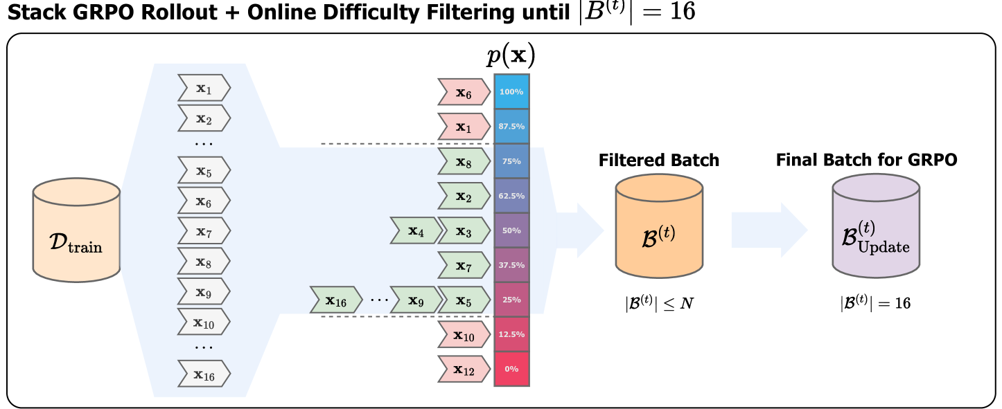
Figure 1: Balanced online difficulty filtering for maximizing the effectiveness of GRPO. With $G$ rollouts for each prompt $\mathbf{x}$, we measure the pass rate $p(\mathbf{x})$ as the average accuracy and filter them by predefined thresholds: e.g., $0.25\leq p(\mathbf{x})\leq 0.75$ in this case. We recursively stack filtered prompts until the train batch size meets the fixed size $N$. We elaborate on the asynchronous implementation in Appendix A.

2 Related Works

Reasoning-oriented reinforcement learning.

Recent advancements demonstrate significant reasoning improvements in LLMs through RL (Havrilla et al., 2024; OpenAI et al., 2024; Lambert et al., 2024; Guo et al., 2025; OLMo et al., 2025; Kumar et al., 2025). OpenAI o1 (OpenAI et al., 2024) initially reported that increasing the compute during RL training and inference improves reasoning performance. DeepSeek R1 (Guo et al., 2025) further found that, in RORL with verifiable rewards, longer responses correlate with better reasoning. Concurrent studies (Team et al., 2025; Hou et al., 2025; Luo et al., 2025) employed algorithms, such as GRPO (Shao et al., 2024) or RLOO (Ahmadian et al., 2024), relying on advantage estimation via multiple response samples rather than PPO-like value networks. Hou et al. (2025) further found that training efficiency improved with increased sampling in RLOO, invoking the need for more sample-efficient training strategies in reasoning-oriented RL.

Difficulty-based curriculum learning.

Curriculum learning has been widely adopted in fine-tuning LLMs to improve training efficiency (Lee et al., 2024; Na¨ır et al., 2024; Team et al., 2025; Cui et al., 2025). Static curricula, i.e., offline data curation with a predetermined task difficulty, have been effective in multiple domains: instruction-tuning (Lee et al., 2024) and coding (Na¨ır et al., 2024; Team et al., 2025; Li et al., 2025) to name a few. In RORL, Team et al. (2025) employs a static difficulty-based curriculum, assigning tasks at fixed difficulty levels to ensure efficient progression. Similarly, Li et al. (2025) selects a high-impact subset of training data based on a “learning impact measure”. Meantime, adaptive curricula dynamically adjust task difficulty based on the learners’ progress, addressing the limitations of static curricula (Florensa et al., 2018; Cui et al., 2025). Specifically, Cui et al. (2025) applied adaptive filtering in reasoning and reported an empirical advantage in reducing reward variance. However, Meng et al. (2025) observed that such dynamic exclusion of examples may destabilize training, as it causes fluctuations in the effective batch size.

3 Preliminaries

Reinforcement learning in language models.

Given the training policy $\pi_{\theta}$ initialized from the reference policy $\pi_{\mathrm{init}}$, reinforcement learning (RL) in language model environment optimizes $\pi_{\theta}$ to maximize the reward assessed by the reward function $r$ (Christiano et al., 2017; Ziegler et al., 2020) through:

$$\max_{\theta}\mathbb{E}_{\mathbf{y}\sim\pi_{\theta}(\cdot|\mathbf{x})}[r(\mathbf{x},\mathbf{y})-\beta\mathbb{D}_{\mathrm{KL}}\left(\pi_{\theta}(\mathbf{y}|\mathbf{x})|\pi_{\mathrm{init}}(\mathbf{y}|\mathbf{x})\right)],$$ (1)

penalizing excessive divergence of $\pi_{\theta}$ with hyperparameter $\beta$ for the input and output token sequences $\mathbf{y}=\{y_{i}\}_{i=1}^{K}$ and $\mathbf{x}=\{x_{i}\}_{i=1}^{M}$. The policy gradient methods like REINFORCE (Williams, 1992) or PPO (Schulman et al., 2017) are often applied, defining token-level reward with the per-token divergence as a final reward (Ziegler et al., 2020; Huang et al., 2024):

$$r(\mathbf{x},\mathbf{y})-\beta\log\frac{\pi_{\theta}(\mathbf{y}|\mathbf{x})}{\pi_{\mathrm{init}}(\mathbf{y}|\mathbf{x})}.$$ (2)

The corresponding optimal policy $\pi^{*}$ is well known to be defined with respect to $\pi_{\mathrm{init}}$ as (Korbak et al., 2022; Go et al., 2023; Rafailov et al., 2023),

$$\pi^{*}(\mathbf{y}|\mathbf{x})=Z(\mathbf{x})\pi_{\mathrm{init}}(\mathbf{y}|\mathbf{x})\exp\left(\frac{1}{\beta}r(\mathbf{x},\mathbf{y})\right),$$ (3)

where $Z(\mathbf{x})$ is the partition function that normalizes the action probability given $\mathbf{x}$.

Group relative policy optimization.

Unlike PPO, recent works propose excluding parameterized value models (Ahmadian et al., 2024; Kazemnejad et al., 2024; Wu et al., 2024), including group relative policy optimization (Shao et al., 2024, GRPO).

GRPO leverages the PPO-style clipped surrogate objective but calculates the policy gradient by weighting the log-likelihood of each trajectory with its group-based advantage, thus removing the need for a critic (Vojnovic and Yun, 2025; Mroueh, 2025). For each prompt, $G$ parallel responses are sampled and their reward $r_{i}$ is used to calculate the advantage $\hat{A}_{i}$:

$$\hat{A}_{i}=\frac{r_{i}-\mathrm{mean}(r_{1},\dots,r_{G})}{\mathrm{std}(r_{1},\dots,r_{G})},$$ (4)

where $\mathrm{mean}(\cdot)$ and $\mathrm{std}(\cdot)$ are the average and standard deviation of the input values. The effectiveness of GRPO is especially highlighted in the tasks with verifiable reward stipulated through the binary reward functions (Lambert et al., 2024; Guo et al., 2025; Wei et al., 2025):

$$r_{\mathrm{acc}}(\mathbf{x},\mathbf{y})=\begin{cases}~~1&\quad\text{if output is correct}\\ ~~0&\quad\text{otherwise.}\end{cases}$$ (5)

4 Learnability in GRPO and Online Difficulty Filtering

In this section, we analyze the learnability of the prompt in RL with language model environments under binary rewards. We show that prompts that are either too easy or too hard yield no learning signal (§4.2), while intermediate ones—characterized by high reward variance—maximize the gradient information (§4.3). Building on these insights, we propose a balanced online difficulty filtering (§4.4 and §4.5) to optimize GRPO training.

4.1 Background: Prompt-level learnability

We begin by recalling the definition of the optimal value function and the partition function in the soft RL setting (Schulman et al., 2018; Richemond et al., 2024):

$$V^{*}(\mathbf{x}):=\beta\log\mathbb{E}_{\mathbf{y}\sim\pi_{\mathrm{init}}(\cdot|\mathbf{x})}\left[\exp\left(\frac{1}{\beta}r\left(\mathbf{x},\mathbf{y}\right)\right)\right]~\mathrm{and}~Z(\mathbf{x})=\exp\left(\frac{1}{\beta}V^{*}(\mathbf{x})\right).$$ (6)

Using $V^{*}(\mathbf{x})$ in Equation (3), the log ratio between the initial policy $\pi_{\mathrm{init}}$ and the optimal policy $\pi^{*}$ can be expressed as:

$$\log\frac{\pi^{*}(\mathbf{y}|\mathbf{x})}{\pi_{\mathrm{init}}(\mathbf{y}|\mathbf{x})}=\frac{1}{\beta}\Big{(}r(\mathbf{x},\mathbf{y})-V^{*}(\mathbf{x})\Big{)}.$$ (7)

Taking the expectation with respect to $\pi_{\mathrm{init}}$ yields:

$$\mathbb{E}_{\mathbf{y}\sim\pi_{\mathrm{init}}(\cdot|\mathbf{x})}\left[\log\frac{\pi^{*}(\mathbf{y}|\mathbf{x})}{\pi_{\mathrm{init}}(\mathbf{y}|\mathbf{x})}\right]=\frac{1}{\beta}\mathbb{E}_{\mathbf{y}\sim\pi_{\mathrm{init}}(\cdot|\mathbf{x})}\left[r(\mathbf{x},\mathbf{y})\right]-\frac{1}{\beta}V^{*}(\mathbf{x}),$$ (8)

where the right-hand side (RHS) represents a soft-RL variant of the advantage function scaled by $\beta^{-1}$ (Haarnoja et al., 2017; Schulman et al., 2018), as $\mathbb{E}_{\pi_{\mathrm{init}}}\left[r(\mathbf{x},\mathbf{y})\right]$ can be interpreted as Q-function. And the left-hand side (LHS) corresponds to the negative reverse KL divergence between $\pi_{\mathrm{init}}$ and $\pi^{*}$ (Rafailov et al., 2024):

$$\mathbb{D}_{\mathrm{KL}}\left(\pi_{\mathrm{init}}(\mathbf{y}|\mathbf{x})|\pi^{*}(\mathbf{y}\,\|\,\mathbf{x})\right)=-\mathbb{E}_{\mathbf{y}\sim\pi_{\mathrm{init}}(\cdot|\mathbf{x})}\left[\log\frac{\pi^{*}(\mathbf{y}|\mathbf{x})}{\pi_{\mathrm{init}}(\mathbf{y}|\mathbf{x})}\right].$$ (9)

Learnability in binary reward case.

For the binary reward $r_{\mathrm{acc}}$ in Equation (5), the reward distribution is Bernoulli with parameter $p(\mathbf{x})$ for prompt $\mathbf{x}$, policy $\pi$, and $\mathbf{y}\sim\pi(\cdot|\mathbf{x})$, which we refer to as “pass rate”:

$$p(\mathbf{x})=\mathbb{E}_{\pi_{\mathrm{init}}}\left[r_{\mathrm{acc}}(\mathbf{x},\mathbf{y})\right],$$ (10)

and variance $p(\mathbf{x})(1-p(\mathbf{x}))$. Here, we categorize the prompts into five categories:

1. Absolute-hard prompts ($\mathbf{x}_{\mathrm{Hard}},~p(\mathbf{x}_{\mathrm{Hard}})=0$)

2. Soft-hard prompts ($\mathbf{x}_{\mathrm{hard}},p(\mathbf{x}_{\mathrm{hard}})=\epsilon$)

3. Intermediate prompts ($\mathbf{x}_{\mathrm{inter}},~\epsilon\leq p(\mathbf{x}_{\mathrm{inter}})\leq 1-\epsilon$)

4. Soft-easy prompts ($\mathbf{x}_{\mathrm{easy}},~p(\mathbf{x}_{\mathrm{easy}})=1-\epsilon$)

5. Absolute-easy prompts ($\mathbf{x}_{\mathrm{Easy}},~p(\mathbf{x}_{\mathrm{Easy}})=1$)

where $\epsilon$ is a small positive constant satisfying $0\ll\epsilon<0.5$. The variance is zero if and only if $p(\mathbf{x})=0$ or $p(\mathbf{x})=1$, corresponding to absolute hard and absolute easy prompts, respectively.

4.2 Case 1: Learnability in absolute prompts

For absolute prompts $\mathbf{x}_{\mathrm{Hard}}$ and $\mathbf{x}_{\mathrm{Easy}}$, both the expected reward and the state value are zero and one, respectively:

$$\begin{cases}~~\mathbb{E}_{\pi_{\mathrm{init}}}\left[r_{\mathrm{acc}}(\mathbf{x},\mathbf{y})\right]=0~~\mathrm{and}~~V^{*}(\mathbf{x})=\beta\log\left(\exp\left(\frac{0}{\beta}\right)\right)=0.&\quad\text{if}~~~\mathbf{x}=\mathbf{x}_{\mathrm{Hard}},\\ ~~\mathbb{E}_{\pi_{\mathrm{init}}}\left[r_{\mathrm{acc}}(\mathbf{x},\mathbf{y})\right]=1~~\mathrm{and}~~V^{*}(\mathbf{x})=\beta\log\left(\exp\left(\frac{1}{\beta}\right)\right)=1.&\quad\text{if}~~~\mathbf{x}=\mathbf{x}_{\mathrm{Easy}}.\end{cases}$$ (11)

By Equation (8), the expected log ratio between $\pi_{\mathrm{init}}$ and $\pi^{*}$ become zero, implying that $\pi_{\mathrm{init}}$ is already optimal regarding the initial model’s capability:

$$\mathbb{D}_{\mathrm{KL}}\left(\pi_{\mathrm{init}}(\mathbf{y}|\mathbf{x})\,\|\,\pi^{*}(\mathbf{y}|\mathbf{x})\right)=0~\mathrm{when}~\mathbf{x}\in\left\{\mathbf{x}_{\mathrm{Hard}},\mathbf{x}_{\mathrm{Easy}}\right\}.$$ (12)

Therefore, absolute-hard and absolute-easy prompts ($p(\mathbf{x})\in\left\{0,1\right\}$) do not contribute useful gradient information during RL training. For GRPO in specific, this is an intuitive result as the advantage $\hat{A}$ in GRPO naturally become zero for every rollout by Equation (4).

4.3 Case 2: Learnability in soft prompts

Next, we show that the prompts with $p(\mathbf{x})\simeq 0.5$ have the largest learnability, thereby preserving the prompts with $\epsilon\leq p(\mathbf{x})\leq 1-\epsilon$ maximize the effectiveness in the RL phase.

Reward variance as a lower bound of optimal divergence.

Regarding $r_{\mathrm{acc}}(\mathbf{x},\mathbf{y})$ with $\mathbf{y}\sim\pi_{\mathrm{init}}(\cdot|\mathrm{x})$ is Bernoulli, we can rewrite $V^{*}(\mathbf{x})$ as:

$$V^{*}(\mathbf{x})=\beta\log\left((1-p(\mathbf{x}))+p(\mathbf{x})\exp\left(\frac{1}{\beta}\right)\right)$$ (13)

by substituting $\mathbb{E}_{\pi_{\mathrm{init}}}\left[\exp\left(r(\mathbf{x},\mathbf{y})/\beta\right)\right]$ through a simple exponential transformation of Bernoulli distribution. With the second order Taylor expansion of $\exp\left(1/\beta\right)$ and applying it to Equation (8), we have:

$$\begin{split}\mathbb{E}_{\mathbf{y}\sim\pi_{\mathrm{init}}(\cdot|\mathbf{x})}\left[\log\frac{\pi^{*}(\mathbf{y}|\mathbf{x})}{\pi_{\mathrm{init}}(\mathbf{y}|\mathbf{x})}\right]&=\frac{p(\mathbf{x})}{\beta}-\log\left((1-p(\mathbf{x}))+p(\mathbf{x})\exp\left(\frac{1}{\beta}\right)\right)\\ &\leq-\frac{1}{2\beta^{2}}p(\mathbf{x})(1-p(\mathbf{x})).\end{split}$$ (14)

Here, RHS is proportional to the variance of $\mathrm{Bernoulli}(p(\mathbf{x}))$. Thus, the reward variance determines the lower bound of the divergence between $\pi_{\mathrm{init}}$ and $\pi^{*}$ given the prompt $\mathbf{x}$:

$$\mathbb{D}_{\mathrm{KL}}\left(\pi_{\mathrm{init}}(\mathbf{y}|\mathbf{x})\,\|\,\pi^{*}(\mathbf{y}|\mathbf{x})\right)\geq\frac{p(\mathbf{x})(1-p(\mathbf{x}))}{2\beta^{2}},$$ (15)

supporting that the prompts with $p(\mathbf{x})\simeq 0.5$ have the largest learnability.

Hence, soft-hard ($p(\mathbf{x_{\mathrm{hard}}})=\epsilon$) and soft-easy ($p(\mathbf{x_{\mathrm{easy}}})=1-\epsilon$) prompts are expected to provide marginal learnability, and intermediate prompts ($\epsilon\leq p(\mathbf{x})\leq 1-\epsilon$) provides the strongest learning signal. See Appendix B for the full derivation.

Algorithm 1 Iterative GRPO with Online Difficulty Filtering

1:Initial policy model $\pi_{\mathrm{init}}$; Reward $r$; Prompts queue $\mathcal{Q}$; Pass rate thresholds $T_{\text{Low}},T_{\text{High}}$; Batch size $N$; Group size $G$; $r_{\text{acc}}$ (5); Visit count $\mathrm{vc}(\mathbf{x})$.

2:$\mathcal{P}_{\text{active}}$: The set of examples currently undergoing asynchronous rollout.

3:$C_{\text{max}}$: The maximum number of examples that can be processed concurrently.

4:function $f_{async}$($\mathbf{x}$)

5:  $\,\{\mathbf{y}_{i}\}_{i=1}^{G}\sim\pi_{\theta}(\cdot\mid\mathbf{x})$

6:  if $\,T_{\text{Low}}\,\leq\,\frac{1}{G}\sum_{i=1}^{G}r_{acc}(\mathbf{x},\mathbf{y}_{i})\,\leq\,T_{\text{High}}$ then

7:   $\mathcal{B}^{(t)}\leftarrow\mathcal{B}^{(t)}\cup\left\{(\mathbf{x},\{\mathbf{y}_{i}\}_{i=1}^{G},\{r(\mathbf{x},\mathbf{y}_{i})\}_{i=1}^{G})\right\}$   

8:  $\mathrm{vc}(\mathbf{x})\leftarrow\mathrm{vc}(\mathbf{x})+1$

9:Initialize policy model $\pi_{\theta}\leftarrow\pi_{\mathrm{init}}$

10:Initialize visit count $\mathrm{vc}(\mathbf{x})\leftarrow 0$ for all $\mathbf{x}\in\mathcal{D}$

11:for $\text{iteration}=1,\ldots,I$ do

12:  Initialize reference model $\pi_{\text{ref}}\leftarrow\pi_{\theta}$

13:  for $\text{step}=1,\ldots,M$ do

14:   Initialize $\mathcal{B}^{(t)}\leftarrow\varnothing$, $\mathcal{P}_{\text{active}}\leftarrow\varnothing$

15:   Sort examples by visit count $\mathcal{Q}\leftarrow\mathrm{sort}_{\mathrm{vc}}(\mathcal{D})$

16:   while $|\mathcal{B}^{(t)}|<N$ do

17:     if $|\mathcal{P}_{\text{active}}|<C_{\text{max}}$ then

18:      $\mathbf{x}\leftarrow\text{nextExample}(\mathcal{Q})$

19:      $\mathcal{P}_{\text{active}}\leftarrow\mathcal{P}_{\text{active}}\cup f_{async}(\mathbf{x})$         

20:   Cancel $\mathcal{P}_{\text{active}}$

21:   Compute $\hat{A}_{i}$ for $\mathbf{y}_{i}$ in $\mathcal{B}^{(t)}$ through group relative advantage estimation (4).

22:   Update the policy model $\pi_{\theta}$ by maximizing the GRPO objective.   

23:Output $\pi_{\theta}$

4.4 Method: online difficulty filtering with fixed batch size

From this vein, it is reasonable to comprise the input prompt set with intermediate difficulty. Furthermore, balanced difficulty in the prompt set encourages balanced model updates for penalizing bad trajectories and reinforcing good trajectories in GRPO (Mroueh, 2025).

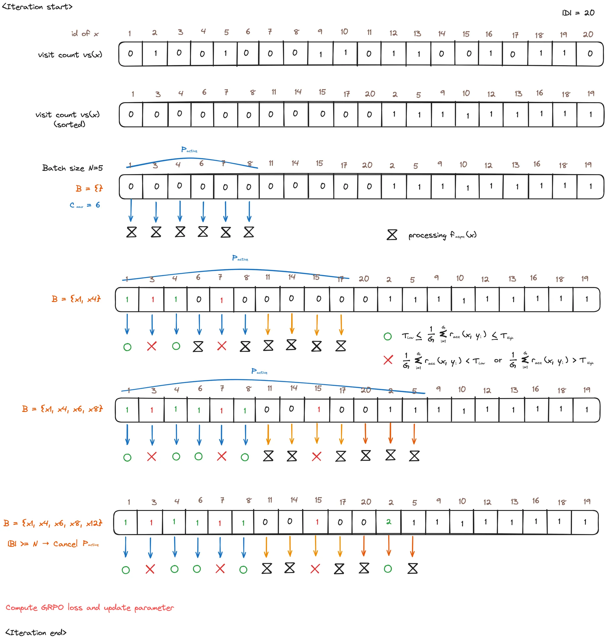
Figure 4: Illustration of the rollout process in the proposed algorithm with online difficulty filtering. Each iteration begins by sorting the dataset based on the visit count $\mathrm{vc(\mathbf{x})}$ of each example $\mathbf{x}$. A batch of unvisited or least-visited prompts is selected, respecting a predefined concurrency limit $C_{\text{max}}$. The asynchronous function $f_{async}$ samples responses from the current policy and evaluates them using the accuracy reward $r_{acc}$. Prompts with a pass rate within the accepted range $[T_{\text{Low}},T_{\text{High}}]$ are added to the training batch. Once the batch $\mathcal{B}$ reaches the target size $N$, any remaining asynchronous jobs in $\mathcal{P}_{\text{active}}$ are canceled. The policy is then updated using the GRPO loss computed over the collected batch.

We analyze an online difficulty filtering approach that ensures a fixed batch size throughout training for a reasoning-oriented agent. Unlike static curricula with predefined difficulty orderings in problems (Yang et al., 2024b; Team et al., 2025; Li et al., 2025), our approach dynamically assesses difficulty on the fly in each training step and applies difficulty filtering logic following the theoretical insights studied in §4. We describe the detailed process in Algorithm 1 and the high-level illustration of the algorithm in Figure 4 in Appendix A.

Online difficulty filtering with sample success rate for learnability.

First, we fill the batch $\mathcal{B}^{(t)}$ of the training step $t$ with filtered examples by measuring the success rate $p(\mathbf{x})$ (10) of each prompt $\mathbf{x}$ using sampled rollouts with size of $G$:

$$\mathcal{B}^{(t)}=\left\{\left(\mathbf{x},\{\mathbf{y}_{i},r_{\mathrm{acc}}(\mathbf{x},\mathbf{y}_{i})\}_{i=1}^{G}\right)\mid T_{\text{Low}}\leq\frac{1}{G}\sum_{i=1}^{G}r_{\mathrm{acc}}(\mathbf{x},\mathbf{y}_{i})\leq T_{\text{High}},~\mathbf{y}_{i}\sim\pi_{\theta_{t}}(\cdot|\mathbf{x})\right\}.$$ (16)

where $T_{\text{Low}}$ and $T_{\text{High}}$ are the predefined difficulty threshold. Here, the sample mean of $r_{acc}(\mathbf{x},\mathbf{y}_{i})$ is an unbiased estimate of $\mathbb{E}_{\mathbf{y}\sim\pi_{\theta_{t}}(\cdot|\mathbf{x})}\left[r_{\mathrm{acc}}(\mathbf{x},\mathbf{y})\right]$ with the sample size of $G$.

Ensuring fixed batch size with asynchronous sampling and efficient batching.

While we showed that online difficulty filtering could maximize learnability in GRPO, naive filtering could result in inconsistent training batch size, leading to training instability and degraded performance (Li et al., 2022). For this reason, we ensure the fixed batch size to $|\mathcal{B}|=N$.

Rollouts for each prompt are sampled asynchronously and in parallel, enabling continuous batching of prompts and rollouts (Daniel et al., 2023; Kwon et al., 2023; Noukhovitch et al., 2025). Each prompt’s visit count, $\mathrm{vc}(\mathbf{x})$, is incremented after generating $G$ rollouts, ensuring it isn’t re-processed in the same iteration. Moreover, the active rollout process $\mathcal{P}_{\text{active}}$ is halted once the batch capacity is reached, allowing prompt training with the collected data. This sampling-based framework is compatible with Monte Carlo methods such as RLOO (Ahmadian et al., 2024) and VinePPO (Kazemnejad et al., 2024).

4.5 Difficulty filtering strategies

We mainly experiment two different difficulty filtering strategies, namely balanced difficulty filtering and skewed difficulty filtering:

1. Balanced difficulty filtering ($\mathrm{mean}(T_{\mathrm{High}},T_{\mathrm{Low}})=0.5$): We set the thresholds to be symmetric to the success rate of $0.5$: e.g., $T_{\mathrm{High}}=0.8$ and $T_{\mathrm{Low}}=0.2$.

2. Skewed difficulty filtering ($\mathrm{mean}(T_{\mathrm{High}},T_{\mathrm{Low}})\neq 0.5$): We set the thresholds asymmetrically, only filtering either easy or hard prompts: e.g., $T_{\mathrm{High}}=0.6$ and $T_{\mathrm{Low}}=0$.

By comparing the two strategies, we test if incorporating either side of extreme success rate cases can boost the performance of online difficulty filtering in GRPO, even though the theoretical learnability for either side has the same lower bound as analyzed in §4.3.

5 Experiments

5.1 Experimental Setup

Supervised fine-tuning.

Before RORL experiments, we fine-tune Qwen2.5-3B base (Yang et al., 2024a) as a cold start, following the approach of Guo et al. (2025). Specifically, we curate 1.1K verified problem-solution pairs, with math problems sampled from NuminaMath (Li et al., 2024) and solutions distilled from DeepSeek-R1 (Guo et al., 2025).

Reinforcement learning.

For RORL, we employ GRPO on top of the SFT checkpoint. In each training step, the model generates 16 rollouts for 16 prompts (drawn from NuminaMath problems) and receives reward based on their correctness. We leave out 1,024 problems as a validation set. We also add a format reward and a language reward as in Guo et al. (2025). Additional training details for SFT and RORL are reported in the Appendix C.

5.2 Experimental design

Different strategies in online difficulty filtering.

Along with the plain GRPO without any prompt filtering, we test the online difficulty filtering with two different strategies introduced in §4.5: i.e., balanced and skewed filtering. For the balanced setting, we test $(T_{\mathrm{Low}},T_{\mathrm{High}})\in\left\{(0,1),(0.1,0.9),(0.2,0.8),(0.3,0.7),(0.4,0.6)\right\}$. For a skewed setting, we sweep $T_{\mathrm{Low}}\in\left\{0,0.2,0.4\right\}$ when $T_{\mathrm{High}}=1$ and $T_{\mathrm{High}}\in\left\{0.6,0.8,1\right\}$ when $T_{\mathrm{Low}}=0$.

Comparison against existing offline filtering methods.

We mainly compare two offline difficulty filtering methods with our approach: offline data curation (Yang et al., 2024b; Cui et al., 2025; Muennighoff et al., 2025; Ye et al., 2025) and offline scheduling (Team et al., 2025; Li et al., 2025). Offline data curation refers to the strategy that filters the problems by their difficulty before training, and offline scheduling additionally orders the training batches accordingly. For both offline strategies, we apply two settings, using Qwen2.5-7B-Instruct (Yang et al., 2024a) or our SFT model, as the difficulty proxies.

Evaluation Benchmarks.

We evaluate pass@1 on challenging math reasoning benchmarks: MATH500 (Hendrycks et al., 2021), AIME (Li et al., 2024), AMC (Li et al., 2024), MinervaMath (Lewkowycz et al., 2022), and OlympiadBench (He et al., 2024) (See Appendix D).

6 Results and Analysis

We first compare different online filtering strategies, balanced and skewed online filtering, in §6.1. Then, we compare with existing offline difficulty filtering methods, analyzing the impact of different difficulty assessment proxies in §6.2.

6.1 Online difficulty filtering strategies: balanced vs skewed filtering

Method	Difficulty Filter	MATH500	AIME	AMC	Minerva.	Olympiad.	Avg.
SFT	-	49.8	0.0	20.5	13.2	17.3	20.2
GRPO w/ Offline Filtering	Curation
	External model	59.6	6.6	27.7	24.3	23.9	28.4
	Initial model	55.6	10.0	28.9	18.8	18.2	26.3
	Schedule
	External model	57.8	10.0	28.9	20.6	21.5	27.8
	Initial model	57.0	3.3	28.9	19.1	24.9	26.7
GRPO w/ Online Filtering (Ours)	Plain
	$0\leq p(\mathbf{x})\leq 1$	57.2	3.3	30.1	18.7	22.2	26.3
	Skewed
	$0<p(\mathbf{x})\leq 1$	57.0	0.0	26.5	19.8	21.4	24.9
	$0.2<p(\mathbf{x})\leq 1$	60.4	0.0	27.7	17.2	24.5	25.9
	$0.4<p(\mathbf{x})\leq 1$	55.8	0.0	21.7	19.9	21.6	23.8
	$0\leq p(\mathbf{x})<1.0$	55.4	3.3	22.8	19.8	19.8	24.2
	$0\leq p(\mathbf{x})<0.8$	56.2	0.0	28.9	17.2	21.7	24.8
	$0\leq p(\mathbf{x})<0.6$	56.2	3.3	26.5	21.3	21.6	25.8
	Balanced
	$0<p(\mathbf{x})<1$	60.8	3.3	31.3	18.0	27.3	27.3
	$0.1<p(\mathbf{x})<0.9$	58.8	13.3	25.3	22.4	22.2	28.4
	$0.2<p(\mathbf{x})<0.8$	62.2	10.0	30.1	20.5	26.3	29.8
	$0.3<p(\mathbf{x})<0.7$	64.6	6.6	28.9	25.4	24.7	30.1
	$0.4<p(\mathbf{x})<0.6$	60.2	6.6	32.8	25.0	24.9	29.9

Table 1: Five math reasoning benchmark evaluation results. “Minerva.” and “Olympiad.” refer to MinervaMath and OlympiadBench. “External” and “Initial” in offline filtering indicate using Qwen2.5-7B-Instruct and our SFT model as difficulty proxy for filtering. $p(\mathbf{x})$ (10) is the pass rate, the average correctness of rollouts. The highest and the second highest scores in each benchmark are highlighted with bold and underline, respectively.

Balanced online difficulty filtering consistently outperforms plain GRPO.

In Table 1, balanced filtering (“Balanced”) outperforms the plain GRPO (“Plain”) on the average score of five challenging math reasoning benchmarks in all five threshold choices. While fine-tuning the SFT checkpoint with plain GRPO without filtering reaches an average score of 26.3%, balanced filtering achieves over 30%, with overall improvements across the benchmarks. For instance, balanced filtering achieved up to 10% point improvement in AIME, which is the most difficult benchmark as shown through the accuracy in Table 1. This supports our theoretical analysis in §4, as online difficulty filtering enhances the effectiveness of GRPO training compared to the plain version without any filtering.

Progressively stricter threshold in balanced filtering incrementally improves performance.

By tightening the pass rate threshold $(T_{\mathrm{Low}},T_{\mathrm{High}})$ for balanced filtering in Table 1, the average score of five benchmarks starts from 27.3% in $(0,1)$, gradually increasing until over 30% in $(0.3,0.7)$. Furthermore, simply removing examples in $(0,1)$ that do not contribute to learning in GRPO results in a slight improvement over the baseline, supporting the analysis in §4.2, i.e., $\hat{A}$ is zero for $(0,1)$. This result suggests that excluding ineffective examples improves both performance and training efficiency by focusing updates on meaningful data.

Skewed online difficulty filtering is less effective than plain GRPO.

While skewed filtering (“Skewed”) in Table 1 improves average performance by up to 5.7% over the SFT checkpoint, plain GRPO with 26.3% outperforms skewed filtering consistently in every threshold choice, which achieves around 24.9% to 25.9%. Overall, maximizing the expected learnability during GRPO training enhances learning in complex reasoning tasks. As discussed in §4.4, balanced filtering emerges as the best choice since it balances between penalizing and reinforcing diverse explorations.

6.2 Difficulty assessment proxy: offline vs online filtering

We apply Off-Diff with implementations from previous works (Yang et al., 2024a), with balanced threshold $(T_{\mathrm{Low}},T_{\mathrm{High}})=(0.2,0.8)$ following the results in §6.1.

Online difficulty filtering yields better learnability than offline methods.

While both offline curation (“Curation”) and offline scheduling (“Schedule”) in Table 1 show marginal improvements over plain GRPO with a maximum $2.1\%$ improvement, balanced online difficulty filtering consistently outperforms offline methods. Within offline methods, using an external difficulty assessment proxy (“External model” in Table 1) exceeded the case using the SFT checkpoint (“initial model”) on average, but with varying results by benchmark.

6.3 Analysis

Online filtering improves training efficiency.

Figure 2 illustrates the progression of the reward in the validation set, plotted against both the training steps (2(a)) and the training time on the wall clock (2(b)). As shown in Figure 2(a), models trained with balanced online difficulty filtering consistently outperform the plain GRPO ($0\leq p(\mathbf{x})\leq 1$) in fewer training steps. This suggests that by filtering out less informative examples, the average learnability within each batch increases, allowing faster learning progress. Interestingly, Figure 2(b) shows that this benefit carries over even when measured by wall-clock time by exceeding plain GRPO’s maximum reward in less training time. However, we also observe that overly aggressive filtering, such as in the case of the $0.4<p(\mathbf{x})<0.6$ setting, can require significantly more rollouts to fill a batch, leading to longer training times overall. These results suggest that online filtering can enable more efficient learning even in real-world settings, as long as overly aggressive filtering is avoided.

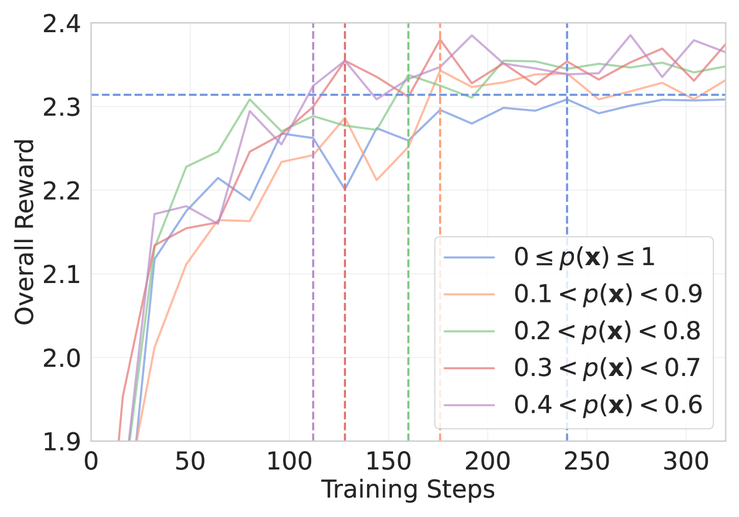
(a) Validation Accuracy over Training Steps

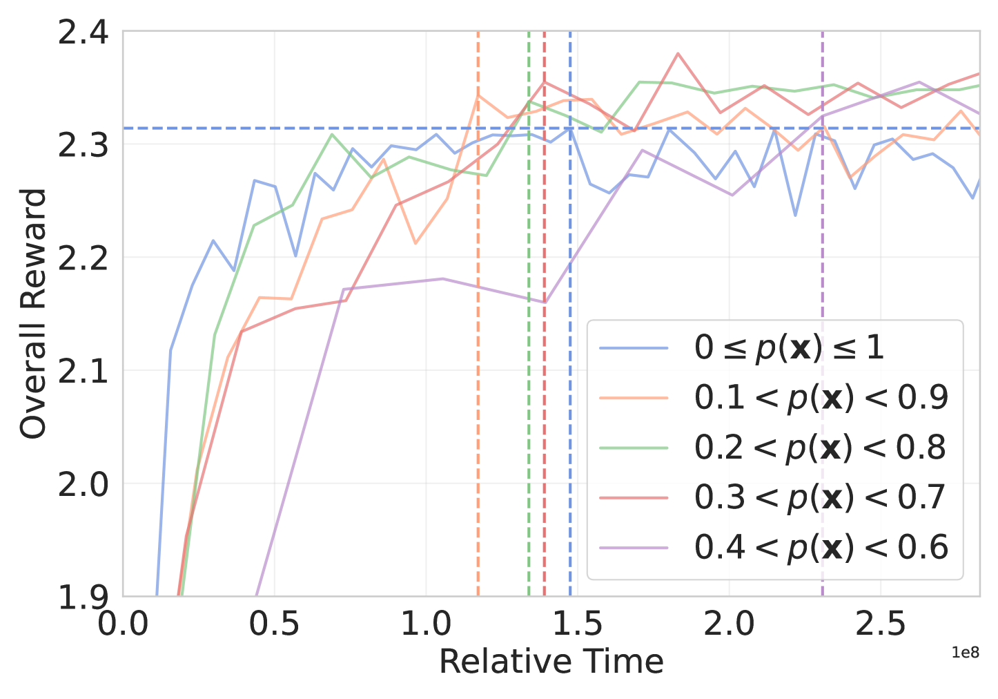
(b) Validation Accuracy over Training Time

Figure 2: Reward as a function of step (2(a)) and relative time (2(b)). The horizontal dashed line indicates the maximum reward achieved by plain GRPO, and the vertical dashed lines indicate when GRPO with each threshold surpasses the plain GRPO’s maximum reward.

Online difficulty filtering adapts to model capability by presenting progressively harder examples.

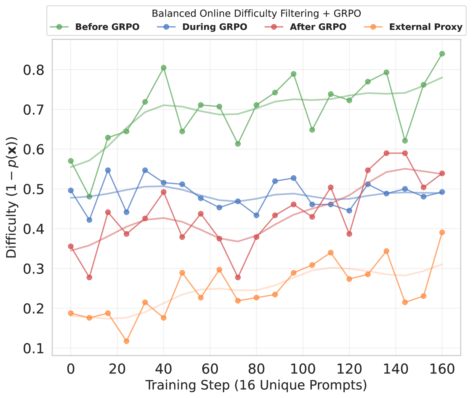
Figure 3: Perceived difficulty per batch curated through balanced online filtering. Defining “difficulty” as $1-p(\mathbf{x})$ , a higher difficulty value implies lower sample accuracy.

In Figure 3, we collect the exact batches curated through balanced online difficulty filtering with $(T_{\mathrm{Low}},T_{\mathrm{High}})=(0.2,0.8)$ and measure the “difficulty” that each model perceives through $1-p(\mathbf{x})$ for four checkpoints: before, during, and after GRPO, along with the external proxy Qwen2.5-7B-Instruct. As anticipated, the checkpoint evaluated during GRPO maintains an average difficulty of around 0.5, dynamically providing suitably challenging examples throughout the training process. However, both before and after GRPO checkpoints perceive incremental difficulty increases across the curated batches, indicating that the training examples become objectively more challenging over time. Moreover, the external proxy model consistently perceives lower difficulty relative to the initial model but higher difficulty than the final trained model (“After GRPO”).

This observation, with the results in Table 1, shows that offline difficulty filtering with external proxies can provide partially meaningful difficulty assessments while not being perfectly aligned to the training model’s capability, shown through marginal improvements in Table 1 compared to plain GRPO. However, the advantage of the balanced online difficulty filtering is still evident in better benchmark results and efficiency.

7 Conclusion

We propose an online curriculum learning framework for reasoning-oriented reinforcement learning (RORL) in large language models (LLMs). By dynamically filtering training examples based on real-time pass rates, our approach ensures that the model focuses on problems within its optimal learning range. Experimental results demonstrate that this method improves sample efficiency and final model performance, outperforming both non-curriculum and offline curriculum baselines. Our findings underscore the importance of adaptive adjustment of training difficulty, paving the way for more effective reinforcement learning strategies for reasoning models.

Appendix A Asynchronous Implementation of Online Difficulty Filtering

We provide a detailed diagram depicting the practical implementation of the online difficulty filtering, especially with the asynchronous setting (Noukhovitch et al., 2025).

Appendix B Learnability in Soft Prompts

Assuming that $r(\mathbf{x},\mathbf{y})\in\left\{0,1\right\}$ given the prompt $\mathbf{x}$ follows a Bernoulli distribution, we have:

$$P(r(\mathbf{x},\mathbf{y})=1)=p(\mathbf{x})~~\mathrm{and}~~P(r(\mathbf{x},\mathbf{y}=0)=1-p(\mathbf{x}).$$ (17)

Defining the inner term $\exp\left(\frac{1}{\beta}r(\mathbf{x},\mathbf{y})\right)$ as the random variable $Y$,

$$Y=\begin{cases}~1&\mathrm{if}~~r(\mathbf{x},\mathbf{y})=0,\\ ~\exp\left(\frac{1}{\beta}\right)&\mathrm{if}~~r(\mathbf{x},\mathbf{y})=1.\end{cases}$$ (18)

Thus, the expectation of $Y$ becomes:

$$\mathbb{E}_{\mathbf{y}\sim\pi_{\mathrm{init}}\left(\cdot|\mathbf{x}\right)}\left[Y\right] =\mathbb{E}_{\mathbf{y}\sim\pi_{\mathrm{init}}\left(\cdot|\mathbf{x}\right)}\left[\exp\left(\frac{1}{\beta}r(\mathbf{x},\mathbf{y})\right)\right]$$ (19)

$$=1\cdot P(r(\mathbf{x},\mathbf{y})=0)+\exp\left(\frac{1}{\beta}\right)\cdot P(r(\mathbf{x},\mathbf{y})=1)$$ (20)

$$=\left(1-p(\mathbf{x})\right)+p\cdot\exp\left(\frac{1}{\beta}\right),$$ (21)

which leads to Equation (13) when applied to $V^{*}(\mathbf{x})$:

$$V^{*}(\mathbf{x})=\beta\log\left((1-p(\mathbf{x}))+p(\mathbf{x})\exp\left(\frac{1}{\beta}\right)\right).$$ (22)

Recall that:

$$\mathbb{E}_{\mathbf{y}\sim\pi_{\mathrm{init}}(\cdot|\mathbf{x})}\left[\log\frac{\pi^{*}(\mathbf{y}|\mathbf{x})}{\pi_{\mathrm{init}}(\mathbf{y}|\mathbf{x})}\right]=\frac{1}{\beta}\mathbb{E}_{\mathbf{y}\sim\pi_{\mathrm{init}}(\cdot|\mathbf{x})}\left[r(\mathbf{x},\mathbf{y})\right]-\frac{1}{\beta}V^{*}(\mathbf{x}),$$ (23)

we can substitute $\mathbb{E}_{\mathbf{y}\sim\pi_{\mathrm{init}}(\cdot|\mathbf{x})}\left[r(\mathbf{x},\mathbf{y})\right]$ with $p\left(\mathbf{x}\right)$ and $V^{*}(\mathbf{x})$ with Equation (22),

$$\mathbb{E}_{\mathbf{y}\sim\pi_{\mathrm{init}}(\cdot|\mathbf{x})}\left[\log\frac{\pi^{*}(\mathbf{y}|\mathbf{x})}{\pi_{\mathrm{init}}(\mathbf{y}|\mathbf{x})}\right]=\frac{p(\mathbf{x})}{\beta}-\log\left((1-p(\mathbf{x}))+p(\mathbf{x})\exp\left(\frac{1}{\beta}\right)\right).$$ (24)

For small $\frac{1}{\beta}$, the Taylor series expansion for the logarithm leads to:

$$\log\left((1-p(\mathbf{x}))+p(\mathbf{x})\exp\left(\frac{1}{\beta}\right)\right) =\log\left((1-p(\mathbf{x}))+p(\mathbf{x})\left(1+\frac{1}{\beta}+\frac{1}{2\beta^{2}}+\ldots\right)\right)$$ (25)

$$=\log\left(1+p(\mathbf{x})\left(\frac{1}{\beta}+\frac{1}{2\beta^{2}}+\ldots\right)\right)$$ (26)

$$\geq\log\left(1+p(\mathbf{x})\left(\frac{1}{\beta}+\frac{1}{2\beta^{2}}\right)\right).$$ (27)

Since $\log\left(1+\epsilon\right)\geq\epsilon-\frac{\epsilon^{2}}{2}$, we can set $\epsilon=p(\mathbf{x})\left(\frac{1}{\beta}+\frac{1}{2\beta^{2}}\right)$:

$$\log\left((1-p(\mathbf{x}))+p(\mathbf{x})\exp\left(\frac{1}{\beta}\right)\right) \geq p(\mathbf{x})\left(\frac{1}{\beta}+\frac{1}{2\beta^{2}}\right)-\frac{1}{2}\left[p(\mathbf{x})\left(\frac{1}{\beta}+\frac{1}{2\beta^{2}}\right)\right]^{2}$$ (28)

$$=\frac{p(\mathbf{x})}{\beta}+\frac{p(\mathbf{x})}{2\beta^{2}}-\frac{p(\mathbf{x})^{2}}{2\beta^{2}}+\mathcal{O}\left(\frac{1}{\beta^{3}}\right)$$ (29)

$$=\frac{p(\mathbf{x})}{\beta}+\frac{p(\mathbf{x})(1-p(\mathbf{x}))}{2\beta^{2}}+\mathcal{O}\left(\frac{1}{\beta^{3}}\right).$$ (30)

Substituting this back into the earlier equation, we obtain:

$$\mathbb{E}_{\mathbf{y}\sim\pi_{\mathrm{init}}(\cdot|\mathbf{x})}\left[\log\frac{\pi^{*}(\mathbf{y}|\mathbf{x})}{\pi_{\mathrm{init}}(\mathbf{y}|\mathbf{x})}\right] \leq\frac{p(\mathbf{x})}{\beta}-\left(\frac{p(\mathbf{x})}{\beta}+\frac{p(\mathbf{x})(1-p(\mathbf{x}))}{2\beta^{2}}\right)$$ (31)

$$=-\frac{p(\mathbf{x})(1-p(\mathbf{x}))}{2\beta^{2}}.$$ (32)

Finally, recalling the definition of KL divergence,

$$\mathbb{D}_{\mathrm{KL}}\left(\pi_{\mathrm{init}}(\mathbf{y}|\mathbf{x})\|\pi^{*}(\mathbf{y}|\mathbf{x})\right)=-\mathbb{E}_{\mathbf{y}\sim\pi_{\mathrm{init}}(\cdot|\mathbf{x})}\left[\log\frac{\pi^{*}(\mathbf{y}|\mathbf{x})}{\pi_{\mathrm{init}}(\mathbf{y}|\mathbf{x})}\right],$$ (33)

We conclude that:

$$\mathbb{D}_{\mathrm{KL}}\left(\pi_{\mathrm{init}}(\mathbf{y}|\mathbf{x})\|\pi^{*}(\mathbf{y}|\mathbf{x})\right)\geq\frac{p(\mathbf{x})(1-p(\mathbf{x}))}{2\beta^{2}},$$ (34)

explicitly establishing the Bernoulli variance scaled by $\frac{1}{2\beta^{2}}$ as a lower bound of the KL divergence between the initial policy and the optimal policy.

Appendix C Training Configurations

All experiments are built on the Qwen2.5-3B base model (Yang et al., 2024a). We integrate DeepSpeed ZeRO-3 (Rajbhandari et al., 2020) optimization in our training pipeline to handle memory and computation efficiently. Both the SFT and RORL stages are conducted on a distributed setup of 8$\times$NVIDIA A100 (80GB) GPUs.

Supervised fine-tuning

We used a learning rate of $5\times 10^{-6}$ and fine-tuned it for 5 epochs. The learning rate schedule was linear, with the first 25 steps used for warm-up. We used a batch size of 21.

Reinforcement learning

We utilize the SGLang (Zheng et al., 2025) framework to accelerate parallel rollout generation, enabling efficient sampling of multiple reasoning trajectories. Training is run for 256 steps, with empirical performance gains saturating after roughly 128 steps. Each update uses 16 sampled rollouts with 16 distinct prompts per batch, followed by a one-step policy update per rollout.

Reward design

To guide the model toward producing responses aligned with the DeepSeek R1 format, we introduce a format reward based on five constraints: (1) the response must begin with a ‘$<$think$>$’ tag, (2) the ‘$<$think$>$’ section must be properly closed with a ‘$<$/think$>$’ tag, (3) the ‘$<$think$>$’ section must be non-empty, (4) the summary section following ‘$<$/think$>$’ must also be non-empty, and (5) the response must terminate with an eot token. Each constraint contributes 0.2 points, resulting in a maximum format reward of 1.0. In addition, we implement a language reward to reduce language mixing, especially given that all prompts during training and evaluation are in English. This reward was computed as the ratio of characters in the response that are alphabetic, symbolic (e.g., mathematical symbols), or whitespace, and ranged from 0 to 1. Lastly, we define an accuracy reward, assigning a score of 1.0 for correct answers and 0.0 for incorrect ones. The total reward is the sum of these three components—format, language, and accuracy—yielding a final reward score between 0 and 3.

Appendix D Evaluation Benchmarks

We employ five different challenging math reasoning benchmarks:

• MATH500 (Hendrycks et al., 2021) consists of 500 problems sampled from Lightman et al. (2023), maintaining topic and difficulty balance.

• AIME (Li et al., 2024, American Invitational Mathematics Examination) uses 30 problems from the 2024 official competition, while AMC (Li et al., 2024, American Mathematics Competitions) includes 40 problems from the 2023 official competition. Both benchmarks consist of contest-level advanced mathematical problems.

• MinervaMath (Lewkowycz et al., 2022) evaluates quantitative reasoning with complex mathematical problems at an undergraduate or Olympiad level.

• OlympiadBench (He et al., 2024) includes 674 open-ended text-only competition problems from a broader set of 8,476 Olympiad and entrance exam questions, specifically using the OE_TO_maths_en_COMP subset.

Inference is conducted via SGLang (Zheng et al., 2025) with top-$p$ set to 0.95, temperature set to 0.6, and the maximum number of output tokens limited to 8,192.

References

- Ahmadian et al. (2024) Arash Ahmadian, Chris Cremer, Matthias Gallé, Marzieh Fadaee, Julia Kreutzer, Olivier Pietquin, Ahmet Üstün, and Sara Hooker. 2024. Back to basics: Revisiting reinforce-style optimization for learning from human feedback in llms. In Proceedings of the 62nd Annual Meeting of the Association for Computational Linguistics (Volume 1: Long Papers), pages 12248–12267.
- Christiano et al. (2017) Paul F Christiano, Jan Leike, Tom Brown, Miljan Martic, Shane Legg, and Dario Amodei. 2017. Deep reinforcement learning from human preferences. In Advances in Neural Information Processing Systems, volume 30. Curran Associates, Inc.
- Cole (1978) Michael Cole. 1978. Mind in society: Development of higher psychological processes. Harvard university press.
- Cui et al. (2025) Ganqu Cui, Lifan Yuan, Zefan Wang, Hanbin Wang, Wendi Li, Bingxiang He, Yuchen Fan, Tianyu Yu, Qixin Xu, Weize Chen, et al. 2025. Process reinforcement through implicit rewards. arXiv preprint arXiv:2502.01456.
- Daniel et al. (2023) Cade Daniel, Chen Shen, Eric Liang, and Richard Liaw. 2023. How continuous batching enables 23x throughput in llm inference while reducing p50 latency.
- Florensa et al. (2018) Carlos Florensa, David Held, Xinyang Geng, and Pieter Abbeel. 2018. Automatic goal generation for reinforcement learning agents. In International conference on machine learning, pages 1515–1528. PMLR.
- Go et al. (2023) Dongyoung Go, Tomasz Korbak, Germán Kruszewski, Jos Rozen, Nahyeon Ryu, and Marc Dymetman. 2023. Aligning language models with preferences through f-divergence minimization. In Proceedings of the 40th International Conference on Machine Learning, ICML’23. JMLR.org.
- Guo et al. (2025) Daya Guo, Dejian Yang, Haowei Zhang, Junxiao Song, Ruoyu Zhang, Runxin Xu, Qihao Zhu, Shirong Ma, Peiyi Wang, Xiao Bi, et al. 2025. Deepseek-r1: Incentivizing reasoning capability in llms via reinforcement learning. arXiv preprint arXiv:2501.12948.
- Haarnoja et al. (2017) Tuomas Haarnoja, Haoran Tang, Pieter Abbeel, and Sergey Levine. 2017. Reinforcement learning with deep energy-based policies. In ICML, pages 1352–1361.
- Havrilla et al. (2024) Alexander Havrilla, Yuqing Du, Sharath Chandra Raparthy, Christoforos Nalmpantis, Jane Dwivedi-Yu, Eric Hambro, Sainbayar Sukhbaatar, and Roberta Raileanu. 2024. Teaching large language models to reason with reinforcement learning. In AI for Math Workshop @ ICML 2024.
- He et al. (2024) Chaoqun He, Renjie Luo, Yuzhuo Bai, Shengding Hu, Zhen Thai, Junhao Shen, Jinyi Hu, Xu Han, Yujie Huang, Yuxiang Zhang, et al. 2024. Olympiadbench: A challenging benchmark for promoting agi with olympiad-level bilingual multimodal scientific problems. In Proceedings of the 62nd Annual Meeting of the Association for Computational Linguistics (Volume 1: Long Papers), pages 3828–3850.
- Hendrycks et al. (2021) Dan Hendrycks, Collin Burns, Saurav Kadavath, Akul Arora, Steven Basart, Eric Tang, Dawn Song, and Jacob Steinhardt. 2021. Measuring mathematical problem solving with the math dataset. In Thirty-fifth Conference on Neural Information Processing Systems Datasets and Benchmarks Track (Round 2).
- Hou et al. (2025) Zhenyu Hou, Xin Lv, Rui Lu, Jiajie Zhang, Yujiang Li, Zijun Yao, Juanzi Li, Jie Tang, and Yuxiao Dong. 2025. Advancing language model reasoning through reinforcement learning and inference scaling. arXiv preprint arXiv:2501.11651.
- Huang et al. (2024) Shengyi Huang, Michael Noukhovitch, Arian Hosseini, Kashif Rasul, Weixun Wang, and Lewis Tunstall. 2024. The n+ implementation details of RLHF with PPO: A case study on TL;DR summarization. In First Conference on Language Modeling.
- Kazemnejad et al. (2024) Amirhossein Kazemnejad, Milad Aghajohari, Eva Portelance, Alessandro Sordoni, Siva Reddy, Aaron Courville, and Nicolas Le Roux. 2024. VinePPO: Accurate credit assignment in RL for LLM mathematical reasoning. In The 4th Workshop on Mathematical Reasoning and AI at NeurIPS’24.
- Korbak et al. (2022) Tomasz Korbak, Hady Elsahar, Germán Kruszewski, and Marc Dymetman. 2022. On reinforcement learning and distribution matching for fine-tuning language models with no catastrophic forgetting. In Advances in Neural Information Processing Systems, volume 35, pages 16203–16220. Curran Associates, Inc.
- Kumar et al. (2025) Aviral Kumar, Vincent Zhuang, Rishabh Agarwal, Yi Su, John D Co-Reyes, Avi Singh, Kate Baumli, Shariq Iqbal, Colton Bishop, Rebecca Roelofs, Lei M Zhang, Kay McKinney, Disha Shrivastava, Cosmin Paduraru, George Tucker, Doina Precup, Feryal Behbahani, and Aleksandra Faust. 2025. Training language models to self-correct via reinforcement learning. In The Thirteenth International Conference on Learning Representations.
- Kwon et al. (2023) Woosuk Kwon, Zhuohan Li, Siyuan Zhuang, Ying Sheng, Lianmin Zheng, Cody Hao Yu, Joseph Gonzalez, Hao Zhang, and Ion Stoica. 2023. Efficient memory management for large language model serving with pagedattention. In Proceedings of the 29th Symposium on Operating Systems Principles, pages 611–626.
- Lambert et al. (2024) Nathan Lambert, Jacob Morrison, Valentina Pyatkin, Shengyi Huang, Hamish Ivison, Faeze Brahman, Lester James V Miranda, Alisa Liu, Nouha Dziri, Shane Lyu, et al. 2024. T” ulu 3: Pushing frontiers in open language model post-training. arXiv preprint arXiv:2411.15124.
- Lee et al. (2024) Bruce W Lee, Hyunsoo Cho, and Kang Min Yoo. 2024. Instruction tuning with human curriculum. In Findings of the Association for Computational Linguistics: NAACL 2024, pages 1281–1309.
- Lewkowycz et al. (2022) Aitor Lewkowycz, Anders Andreassen, David Dohan, Ethan Dyer, Henryk Michalewski, Vinay Ramasesh, Ambrose Slone, Cem Anil, Imanol Schlag, Theo Gutman-Solo, et al. 2022. Solving quantitative reasoning problems with language models. Advances in Neural Information Processing Systems, 35:3843–3857.
- Li et al. (2022) Conglong Li, Minjia Zhang, and Yuxiong He. 2022. The stability-efficiency dilemma: Investigating sequence length warmup for training GPT models. In Advances in Neural Information Processing Systems.
- Li et al. (2024) Jia Li, Edward Beeching, Lewis Tunstall, Ben Lipkin, Roman Soletskyi, Shengyi Huang, Kashif Rasul, Longhui Yu, Albert Q Jiang, Ziju Shen, et al. 2024. Numinamath: The largest public dataset in ai4maths with 860k pairs of competition math problems and solutions. Hugging Face repository, 13:9.
- Li et al. (2025) Xuefeng Li, Haoyang Zou, and Pengfei Liu. 2025. Limr: Less is more for rl scaling. arXiv preprint arXiv:2502.11886.
- Lightman et al. (2023) Hunter Lightman, Vineet Kosaraju, Yuri Burda, Harrison Edwards, Bowen Baker, Teddy Lee, Jan Leike, John Schulman, Ilya Sutskever, and Karl Cobbe. 2023. Let’s verify step by step. In The Twelfth International Conference on Learning Representations.
- Luo et al. (2025) Michael Luo, Sijun Tan, Justin Wong, Xiaoxiang Shi, William Y. Tang, Manan Roongta, Colin Cai, Jeffrey Luo, Tianjun Zhang, Li Erran Li, Raluca Ada Popa, and Ion Stoica. 2025. Deepscaler: Surpassing o1-preview with a 1.5b model by scaling rl. https://pretty-radio-b75.notion.site/DeepScaleR-Surpassing-O1-Preview-with-a-1-5B-Model-by-Scaling-RL-19681902c1468005bed8ca303013a4e2. Notion Blog.
- Meng et al. (2025) Fanqing Meng, Lingxiao Du, Zongkai Liu, Zhixiang Zhou, Quanfeng Lu, Daocheng Fu, Botian Shi, Wenhai Wang, Junjun He, Kaipeng Zhang, et al. 2025. Mm-eureka: Exploring visual aha moment with rule-based large-scale reinforcement learning. arXiv preprint arXiv:2503.07365.
- Mroueh (2025) Youssef Mroueh. 2025. Reinforcement learning with verifiable rewards: Grpo’s effective loss, dynamics, and success amplification.
- Muennighoff et al. (2025) Niklas Muennighoff, Zitong Yang, Weijia Shi, Xiang Lisa Li, Li Fei-Fei, Hannaneh Hajishirzi, Luke Zettlemoyer, Percy Liang, Emmanuel Candès, and Tatsunori Hashimoto. 2025. s1: Simple test-time scaling. arXiv preprint arXiv:2501.19393.
- Na¨ır et al. (2024) Marwa Naïr, Kamel Yamani, Lynda Said Lhadj, and Riyadh Baghdadi. 2024. Curriculum learning for small code language models. In 62nd Annual Meeting of the Association for Computational Linguistics, ACL 2024, pages 531–542. Association for Computational Linguistics (ACL).
- Noukhovitch et al. (2025) Michael Noukhovitch, Shengyi Huang, Sophie Xhonneux, Arian Hosseini, Rishabh Agarwal, and Aaron Courville. 2025. Faster, more efficient RLHF through off-policy asynchronous learning. In The Thirteenth International Conference on Learning Representations.
- OLMo et al. (2025) Team OLMo, Pete Walsh, Luca Soldaini, Dirk Groeneveld, Kyle Lo, Shane Arora, Akshita Bhagia, Yuling Gu, Shengyi Huang, Matt Jordan, Nathan Lambert, Dustin Schwenk, Oyvind Tafjord, Taira Anderson, David Atkinson, Faeze Brahman, Christopher Clark, Pradeep Dasigi, Nouha Dziri, Michal Guerquin, Hamish Ivison, Pang Wei Koh, Jiacheng Liu, Saumya Malik, William Merrill, Lester James V. Miranda, Jacob Morrison, Tyler Murray, Crystal Nam, Valentina Pyatkin, Aman Rangapur, Michael Schmitz, Sam Skjonsberg, David Wadden, Christopher Wilhelm, Michael Wilson, Luke Zettlemoyer, Ali Farhadi, Noah A. Smith, and Hannaneh Hajishirzi. 2025. 2 olmo 2 furious.
- OpenAI et al. (2024) OpenAI, :, Aaron Jaech, Adam Kalai, Adam Lerer, Adam Richardson, Ahmed El-Kishky, Aiden Low, Alec Helyar, Aleksander Madry, Alex Beutel, Alex Carney, Alex Iftimie, Alex Karpenko, Alex Tachard Passos, Alexander Neitz, Alexander Prokofiev, Alexander Wei, Allison Tam, Ally Bennett, Ananya Kumar, Andre Saraiva, Andrea Vallone, Andrew Duberstein, Andrew Kondrich, Andrey Mishchenko, Andy Applebaum, Angela Jiang, Ashvin Nair, Barret Zoph, Behrooz Ghorbani, Ben Rossen, Benjamin Sokolowsky, Boaz Barak, Bob McGrew, Borys Minaiev, Botao Hao, Bowen Baker, Brandon Houghton, Brandon McKinzie, Brydon Eastman, Camillo Lugaresi, Cary Bassin, Cary Hudson, Chak Ming Li, Charles de Bourcy, Chelsea Voss, Chen Shen, Chong Zhang, Chris Koch, Chris Orsinger, Christopher Hesse, Claudia Fischer, Clive Chan, Dan Roberts, Daniel Kappler, Daniel Levy, Daniel Selsam, David Dohan, David Farhi, David Mely, David Robinson, Dimitris Tsipras, Doug Li, Dragos Oprica, Eben Freeman, Eddie Zhang, Edmund Wong, Elizabeth Proehl, Enoch Cheung, Eric Mitchell, Eric Wallace, Erik Ritter, Evan Mays, Fan Wang, Felipe Petroski Such, Filippo Raso, Florencia Leoni, Foivos Tsimpourlas, Francis Song, Fred von Lohmann, Freddie Sulit, Geoff Salmon, Giambattista Parascandolo, Gildas Chabot, Grace Zhao, Greg Brockman, Guillaume Leclerc, Hadi Salman, Haiming Bao, Hao Sheng, Hart Andrin, Hessam Bagherinezhad, Hongyu Ren, Hunter Lightman, and Hyung Won Chung et al. 2024. Openai o1 system card.
- Rafailov et al. (2024) Rafael Rafailov, Joey Hejna, Ryan Park, and Chelsea Finn. 2024. From $r$ to $q^*$: Your language model is secretly a q-function. In First Conference on Language Modeling.
- Rafailov et al. (2023) Rafael Rafailov, Archit Sharma, Eric Mitchell, Christopher D Manning, Stefano Ermon, and Chelsea Finn. 2023. Direct preference optimization: Your language model is secretly a reward model. In Thirty-seventh Conference on Neural Information Processing Systems.
- Rajbhandari et al. (2020) Samyam Rajbhandari, Jeff Rasley, Olatunji Ruwase, and Yuxiong He. 2020. Zero: Memory optimizations toward training trillion parameter models. In SC20: International Conference for High Performance Computing, Networking, Storage and Analysis, pages 1–16. IEEE.
- Richemond et al. (2024) Pierre Harvey Richemond, Yunhao Tang, Daniel Guo, Daniele Calandriello, Mohammad Gheshlaghi Azar, Rafael Rafailov, Bernardo Avila Pires, Eugene Tarassov, Lucas Spangher, Will Ellsworth, Aliaksei Severyn, Jonathan Mallinson, Lior Shani, Gil Shamir, Rishabh Joshi, Tianqi Liu, Remi Munos, and Bilal Piot. 2024. Offline regularised reinforcement learning for large language models alignment.
- Schulman et al. (2018) John Schulman, Xi Chen, and Pieter Abbeel. 2018. Equivalence between policy gradients and soft q-learning.
- Schulman et al. (2017) John Schulman, Filip Wolski, Prafulla Dhariwal, Alec Radford, and Oleg Klimov. 2017. Proximal policy optimization algorithms. arXiv preprint arXiv:1707.06347.
- Shao et al. (2024) Zhihong Shao, Peiyi Wang, Qihao Zhu, Runxin Xu, Junxiao Song, Xiao Bi, Haowei Zhang, Mingchuan Zhang, YK Li, Y Wu, et al. 2024. Deepseekmath: Pushing the limits of mathematical reasoning in open language models. arXiv preprint arXiv:2402.03300.
- Team et al. (2025) Kimi Team, Angang Du, Bofei Gao, Bowei Xing, Changjiu Jiang, Cheng Chen, Cheng Li, Chenjun Xiao, Chenzhuang Du, Chonghua Liao, et al. 2025. Kimi k1. 5: Scaling reinforcement learning with llms. arXiv preprint arXiv:2501.12599.
- Tzannetos et al. (2023) Georgios Tzannetos, Bárbara Gomes Ribeiro, Parameswaran Kamalaruban, and Adish Singla. 2023. Proximal curriculum for reinforcement learning agents. arXiv preprint arXiv:2304.12877.
- Vojnovic and Yun (2025) Milan Vojnovic and Se-Young Yun. 2025. What is the alignment objective of grpo?
- Wei et al. (2025) Yuxiang Wei, Olivier Duchenne, Jade Copet, Quentin Carbonneaux, Lingming Zhang, Daniel Fried, Gabriel Synnaeve, Rishabh Singh, and Sida I. Wang. 2025. Swe-rl: Advancing llm reasoning via reinforcement learning on open software evolution.
- Williams (1992) Ronald J Williams. 1992. Simple statistical gradient-following algorithms for connectionist reinforcement learning. Machine learning, 8:229–256.
- Wu et al. (2024) Tianhao Wu, Banghua Zhu, Ruoyu Zhang, Zhaojin Wen, Kannan Ramchandran, and Jiantao Jiao. 2024. Pairwise proximal policy optimization: Language model alignment with comparative RL. In First Conference on Language Modeling.
- Yang et al. (2024a) An Yang, Baosong Yang, Beichen Zhang, Binyuan Hui, Bo Zheng, Bowen Yu, Chengyuan Li, Dayiheng Liu, Fei Huang, Haoran Wei, et al. 2024a. Qwen2. 5 technical report. arXiv preprint arXiv:2412.15115.
- Yang et al. (2024b) An Yang, Beichen Zhang, Binyuan Hui, Bofei Gao, Bowen Yu, Chengpeng Li, Dayiheng Liu, Jianhong Tu, Jingren Zhou, Junyang Lin, Keming Lu, Mingfeng Xue, Runji Lin, Tianyu Liu, Xingzhang Ren, and Zhenru Zhang. 2024b. Qwen2.5-math technical report: Toward mathematical expert model via self-improvement.
- Ye et al. (2025) Yixin Ye, Zhen Huang, Yang Xiao, Ethan Chern, Shijie Xia, and Pengfei Liu. 2025. Limo: Less is more for reasoning. arXiv preprint arXiv:2502.03387.
- Zheng et al. (2025) Lianmin Zheng, Liangsheng Yin, Zhiqiang Xie, Chuyue Livia Sun, Jeff Huang, Cody Hao Yu, Shiyi Cao, Christos Kozyrakis, Ion Stoica, Joseph E Gonzalez, et al. 2025. Sglang: Efficient execution of structured language model programs. Advances in Neural Information Processing Systems, 37:62557–62583.
- Ziegler et al. (2020) Daniel M. Ziegler, Nisan Stiennon, Jeffrey Wu, Tom B. Brown, Alec Radford, Dario Amodei, Paul Christiano, and Geoffrey Irving. 2020. Fine-tuning language models from human preferences.