Metric spaces with small rough angles and the rectifiability of rough self-contracting curves
Abstract.
The small rough angle () condition, introduced by Zolotov in arXiv:1804.00234, captures the idea that all angles formed by triples of points in a metric space are small. In the first part of the paper, we develop the theory of metric spaces satisfying the condition for some . Given a metric space and , the space satisfies the condition. We prove a quantitative converse up to bi-Lipschitz change of the metric. We also consider metric spaces which are free (there exists a uniform upper bound on the cardinality of any subset) or full (there exists an infinite subset). Examples of free spaces include Euclidean spaces, finite-dimensional Alexandrov spaces of non-negative curvature, and Cayley graphs of virtually abelian groups; examples of full spaces include the sub-Riemannian Heisenberg group, Laakso graphs, and Hilbert space. We study the existence or nonexistence of subsets for in metric spaces for .
In the second part of the paper, we apply the theory of metric spaces with small rough angles to study the rectifiability of roughly self-contracting curves. In the Euclidean setting, this question was studied by Daniilidis, Deville, and the first author using direct geometric methods. We show that in any free metric space , there exists so that any bounded roughly -self-contracting curve in , , is rectifiable. The proof is a generalization and extension of an argument due to Zolotov, who treated the case , i.e., the rectifiability of self-contracting curves in free spaces.
1. Introduction
1.1. Overview
Our goals in this paper are twofold. First, we provide a gentle introduction to the theory of metric spaces with small rough angles, a condition introduced by Zolotov in [41]. The condition, , on a metric space is a strengthened form of the triangle inequality which implies, in particular, that all metric angles formed by triples of points in are bounded away from (quantitatively in terms of ). In particular, we discuss the relationship between this condition and the snowflaking operation , . We go on to consider metric spaces which are either free or full for some . The former condition requires the existence of a uniform upper bound on the cardinality of any subset of , while the latter condition asserts the existence of an infinite subset. These conditions were also introduced by Zolotov in [41], see also [24]. Euclidean space is free for any and any ; this follows from a classical theorem of geometric combinatorics due to Erdös and Füredi. We present various examples of spaces with these properties, and we study the existence of large subsets in snowflaked metric spaces.
Next, we establish the rectifiability of a class of metrically defined curves in free metric spaces, known as roughly self-contracting curves. Self-contracting curves have been introduced by Daniilidis, Ley and Sabourau [9] in connection with the theory of gradient flows for convex potential functions, and the rectifiability of such curves has been established by various authors in spaces of increasing generality. By now it is known that bounded, self-contracting curves are rectifiable in arbitrary Riemannian manifolds, and also in metric spaces satisfying suitable synthetic curvature bounds (à la Alexandrov). In [41], Zolotov establishes the rectifiability of bounded, self-contracting curves in any metric space which is free for some . For each , the class of roughly -self-contracting curves is defined via a metric inequality, similar to the condition but imposed only on ordered triples of points chosen along the curve. These classes interpolate between the class of geodesic curves and all possible curves, in the following sense: roughly -self-contracting curves are precisely the geodesics, while any curve is roughly -self-contracting. A curve is roughly -self-contracting if and only if it is self-contracting. We extend Zolotov’s result to cover roughly -self-contracting curves for some positive choices of .
An important ancillary aim of this paper is to advertise free metric spaces as natural objects for study within the framework of analysis in metric spaces. In this paper, we highlight connections to topics such as bi-Lipschitz embeddability, rectifiability, and the snowflaking operation. We also aim to increase the visibility of the results obtained by Zolotov in [41], and especially to showcase the interesting methodology in his proofs. The second part of this paper is inspired heavily by the results and techniques in [41].
1.2. Statement of main results
For , a metric space is said to satisfy the condition111The acronym stands for small rough angles. if for all . The class of spaces increases as increases, with the condition coinciding with the well-known concept of ultrametric and the condition coinciding with the usual triangle inequality. Geometrically, the condition on a metric space implies an upper bound on all metric angles formed by triples of points in (Remark 2.4).
An alternate one-parameter family of conditions interpolating between the class of ultrametric spaces and the class of all metric spaces was studied by the second author and Wu in [39]. For , is said to be an metric space if for all . When , the metric condition limits to the usual ultrametric condition . For any , the expression defines an metric on , , and the transformation is commonly referred to as the snowflaking transformation in the literature. In this paper, following the terminology in [39], we call a metric space a -snowflake if is bi-Lipschitz equivalent to an metric on . Building on observations by Le Donne, Rajala, and Walsberg [23] and Zolotov [41], we note that the metric space , , satisfies the condition for any metric space . The value is best possible for such a conclusion with no further restrictions on (Example 2.11). We devote some space to consideration of the converse assertion, namely, whether or not the validity of an condition implies that the underlying metric is an metric for some . Such a conclusion is true for any finite set, but we give examples of infinite metric spaces for which such a converse statement is false. However, the situation is clarified if we allow for a bi-Lipschitz change of the metric. This is the content of our first main theorem.
Theorem 1.1.
For any metric space , the following conditions are quantitatively equivalent:
-
(i)
There exists a metric on bi-Lipschitz equivalent to and so that is a metric space.
-
(ii)
There exists a metric on bi-Lipschitz equivalent to and so that satisfies the condition.
Recall that two metrics and on a set are said to be bi-Lipschitz equivalent if there exists a constant so that
For a given choice of , a metric space is said to be free if there exists so that any subset of has cardinality at most , while is said to be full if it contains an infinite subset. A result in geometric combinatorics due to Erdös and Füredi (Proposition 2.7) implies that is free for each . Other examples of free spaces include finite-dimensional Alexandrov spaces of non-negative curvature and Cayley graphs of virtually abelian groups. Moreover, all free spaces are doubling, [24, Theorem 6]. On the other hand, spaces containing large snowflaked subsets are full in view of Theorem 1.1. For example, the sub-Riemannian Heisenberg group is full, since the -axis in is isometric to a snowflaked copy of the real line. Other examples of full spaces include the standard Laakso graphs (see [21] and Example 3.6). An interesting class of full examples is provided by a family of metric trees whose construction depends on a sequence of real numbers (Example 3.5). How one chooses the sequence can influence the doubling property, the bi-Lipschitz embeddability of the space, and the possibility of finding a bounded unrectifiable self-contracting curve (Proposition 3.19). Infinite-dimensional spaces also provide examples of full spaces; for instance, Hilbert space is full (Example 3.4).
Earlier, we noted that the snowflaked space satisfies the condition, and that the value was best possible for such a conclusion without further restrictions on . However, in contrast with this fact we prove the following result on the existence of large subsets in snowflaked metric spaces for arbitrary positive choices of .
Theorem 1.2.
Let be any metric space containing a nontrivial geodesic curve, and let . Then is full for each .
In fact, we can prove an even stronger conclusion: any such metric space contains not only an infinite subset satisfying the condition, but contains Cantor-type subsets of positive Hausdorff dimension satisfying that condition (Proposition 3.16).
In the second part of the paper, we connect the theory of free metric spaces to the rectifiability of roughly self-contracting curves, a class of curves introduced in [7]. A curve is called a rough -self-contracting curve if for every in we have
The class of roughly self-contracting curves is a natural generalization of the class of self-contracted curves () introduced in [9]. Due to the role of self-contraction in the theory of gradient flows for convex potentials, it is of interest to know when such curves are rectifiable. In the Euclidean setting, solutions to gradient flow systems governed by a convex or quasi-convex function are steepest descent curves that satisfy the self-contractedness property. The rectifiability of such curves is linked to the convergence of various central optimization algorithms in convex analysis or graph theory (see [9], [6], [7], and the references therein). It is worth highlighting that the theory of gradient flows has also been studied in a purely metric context, through a variational inequality based on a metric characterization of the curves of maximum slope (see the seminal book by Ambrosio, Gigli, and Savaré [1]). In certain metric spaces, such as spaces, gradient curves are also known to be self-contracting ([24, Proposition 30]).
Rectifiability of self-contracting curves is known to hold in Euclidean space [9], [6], [29], in finite dimensional normed spaces [35], [26], on Riemannian manifolds [8] and in a certain class of spaces [32]. Zolotov [41] establishes the same conclusion for self-contracting curves in free metric spaces for a suitable range of (see also [24]). Rectifiability of rough -self-contracting curves in for was established in [7], but the topic has not been considered in any other settings to date. The main result of the second part of this paper generalizes the theorem of Zolotov [41] and the results in [7] to the setting of roughly self-contracting curves.
Theorem 1.3.
Let and let be an free metric space. Then there exists so that any bounded, rough -self-contracting curve in , with is rectifiable.
We end this introduction with an outline of the paper. In section 2 we give basic facts about metric spaces satisfying the condition. In particular, in subsection 2.2 we discuss the connection between the condition and snowflaking, and we prove Theorem 1.1. The Euclidean bi-Lipschitz embeddability of metric spaces with small rough angles follows from Theorem 1.1 and the Assouad Embedding Theorem. We comment briefly on this topic in subsection 2.3. Section 3 concerns subsets of metric spaces, especially snowflake metric spaces, satisfying the condition. Here we give the proof of Theorem 1.2. We also present a number of examples of free and full metric spaces.
The second part of the paper consists of section 4, where we study the rectifiability of roughly self-contracting curves in free metric spaces. A substantial portion of this section is devoted to the proof of Theorem 1.3, which closely follows the innovative argument put forward by Zolotov [41] in the self-contracting category.
We conclude the paper with a list of open questions (section 5) and two appendices. In Appendix A (section 6) , we provide an example, due to Hytönen, of a doubling metric space which is neither -free nor -full. In Appendix B (section 7), we present a partial result in support of one of the open questions mentioned in section 5.
Acknowledgements: We would like to thank Zoltán Balogh and Efstathios Chrontsios Garitsis for helpful discussions on the subject of this paper. We are also grateful to Tuomas Hytönen for feedback, and for permission to include his example of a doubling metric space which is neither free nor full.
2. Metric spaces with small rough angles
2.1. Definitions
Le Donne, Rajala, and Walsberg proved in [23] that a snowflake of a metric space isometrically embeds into a finite-dimensional normed space if and only if the space is finite. The main idea behind the proof was to observe that, in a space with a snowflake metric, the angles formed by any three points must be roughly small. On the other hand, by a result of Erdös and Füredi [14], in any Euclidean subset with sufficiently many points, some triple of points must form a large angle. Based on [23], Zolotov in [41] defined a class of metric spaces that satisfy a stronger form of the triangle inequality, while also capturing the idea that all angles within the space are roughly small.
Definition 2.1 (Small rough angles condition).
Let . A metric space satisfies the condition (small rough angles with parameter ) if
| (2.1) |
Condition (2.1) weakens as increases, so every space satisfying the condition also satisfies the condition for each . Every metric space satisfies the condition, while the condition characterizes the class of ultrametric spaces.
Remark 2.2.
In principle, one might also consider (2.1) for values .222In section 4 we will consider an analogous notion (rough -self-contractivity) for ordered sets of points and for curves, in which a condition similar to (2.1) is imposed but only for ordered triples of points. The notion of rough -self-contracting ordered set or curve makes sense and is nontrivial for all , with the rough -self-contracting condition characterizing collinear sets or geodesic curves. By way of contrast, the condition that a metric space satisfy the condition imposes a restriction on all possible permutations of any triple of points. However, it is easy to see that no space with more than two elements can satisfy the condition for any . Assume that satisfies the condition with , and suppose that contains at least three distinct elements . Without loss of generality, assume that . Interchanging the roles of and if necessary, we may assume from (2.1) that . Then and hence . This contradicts the assumption that , , and are distinct.
Remark 2.3.
In general, it can be difficult to find sets satisfying an condition. For example, no set of three points on the real line satisfies the condition for any . To see this, assume and assume without loss of generality that . Let us determine where a third point satisfying an condition should be located. Without loss of generality, we can assume that . If for some then . In order for (2.1) to be satisfied, we should have
Hence, either (implying ) or (implying ), and both cases lead to a contradiction.
Although we presented this example in the real line, the proof shows that the same conclusion holds true in any metric space that contains three collinear points.
Remark 2.4.
Let us motivate why Definition 2.1 inherently reflects the idea that all angles are roughly small, depending on the parameter . Any set of three points in a metric space can be isometrically embedded into . Let us consider a comparison triangle , with angles and . Assume that . Then the validity of (2.1) for some given implies that , whence
On the other hand, the law of cosines and the previous inequality imply that
and so the angle is less or equal than . The same argument applies to the other two angles. Hence any angle formed by any three points in is less than or equal to . In particular, if satisfies the condition then every angle is at most .
Remark 2.5.
We emphasize that the fact that all angles are less than or equal to does not imply that the space satisfies the condition. For an example, let be a -point subset of where and . In this case, , , and all angles are less than or equal to . However, is not an ultrametric space. Recall that, in any ultrametric space, every triangle is an acute isosceles triangle, that is, a triangle with two equal sides with the third side of length less than or equal to that of the other two.
Remark 2.6.
Furthermore, a metric space satisfying an condition for some need not have the property that all triangles are acute. Choose such that . Let and let be a -point metric space such that and . This space trivially satisfies the condition. However, by the law of cosines, the euclidean angle in the comparison triangle satisfies
We recall the result of Erdös–Füredi [14, Theorem 4.3] alluded to above: in , sufficiently large subsets necessarily form at least one large angle. In [23, Theorem 1.1], this result is used in the context of finite-dimensional normed spaces with the help of the John Ellipsoid Theorem.
Proposition 2.7 (Erdös–Füredi).
For any and there exists so that if has cardinality at least , then there are distinct such that .
According to [14, Theorem 4.3], the optimal choice of satisfies
| (2.2) |
The proof in [14] is combinatorial; a purely geometric proof for Proposition 2.7 (which yields a non-sharp value for ) was given by Käenmäki and Suomala in [17].
Corollary 2.8.
For each and , there exists so that if satisfies the condition, then contains at most elements.
Remark 2.9.
The cardinality of any set of points in , , satisfying the () condition provides a lower bound for the maximal number of points in such that all angles determined by any triple of points are less or equal to a certain angle (). For example, a regular simplex in (comprising points) trivially satisfies the condition for any . Moreover, the vertices of a regular simplex together with the center of its circumscribed spFhere form a set of points that satisfies the condition.
We will return to this circle of ideas in Section 3, where we introduce the notions of free and full metric spaces. Phrased in that language, Corollary 2.8 says that is an free metric space for each and . Before we take up that discussion, we consider how the snowflaking transformation of a metric affects the validity of the condition.
2.2. Small rough angles and the snowflaking transformation on metric spaces
In [23, Theorem 1.1], the authors establish that for a given metric space and , the snowflaked metric space satisfies the condition with . The following result improves this observation and gives the sharp value of .
Lemma 2.10.
Let be a metric space and . Then satisfies the condition.
Proof.
Let and . Let us denote , and . Without loss of generality we can assume . Since it is enough to find the smallest possible such that
Because , the maximum is attained in the second term. Dividing the expression by and setting , the problem reduces to finding such that the function
satisfies for . If we impose we obtain . Because , is continuous, and has a single maximum in the interval it is clear that for , for and the result follows. ∎
In particular, since for each , we recover the conclusion of [23]. The subsequent example demonstrates that Lemma 2.10 is sharp.
Example 2.11.
Let be an arithmetic sequence in , with and . Then and for any , .
A natural question is whether the converse of Lemma 2.10 is true; specifically, if the condition implies that the metric coincides with a fractional power of another metric. The following example shows that this is not the case.
Example 2.12.
Let where , and equip with the following metric:
Fix and a sequence with and . Let , , be points in with the property that for fixed , the points , , form the vertices of a triangle with sides of Euclidean length , , and . Let be the subset consisting of all points of the form , where and .
We first verify that satisfies the condition. Let , , and be distinct elements of . If then and the condition is clearly satisfied for any permutation of the three points. On the other hand, if , , and are not all equal then without loss of generality assume that and . In this case the triangle formed by the points , , and is an isoceles triangle with two sides of length and a third side of length less than or equal to . Such triangle is then an acute isosceles triangle in the sense of Remark 2.5, and hence this triple of points satisfies the condition and consequently also satisfies the condition.
Finally, we show that fails to be a metric space for any . Suppose that is a metric on for some . Then the triangle inequality
| (2.3) |
Using the inequality valid for and , we obtain and hence
Since and we get a contradiction.
Remark 2.13.
The metric space defined in the previous example is separable, and hence embeds isometrically in by the Fréchet embedding theorem. It is natural to ask if any examples illustrating this conclusion can be provided which lie in a nicer Banach space, e.g., for some or even . In Appendix B (section 6), we give an example of a set of this type, but only for a restricted range of values of . The construction is essentially the same as in Example 2.12, but rather than abstractly defining the distance between elements of distinct triangles to be equal to , the triangles are arranged in a sequence of orthogonal two-dimensional subspaces of , lying near the vertices of an infinite-dimensional equilateral simplex.
See section 5 for further questions and remarks.
Next, we show that if is a finite metric space, then the converse of Lemma 2.10 is true.
Proposition 2.14.
If a finite set satisfies the condition with respect to a metric , then the metric coincides with a fractional power of another metric.
Proof.
Let be a metric space. We can construct comparison triangles () with sides of Euclidean lengths , and for every , where . Fix a triangle with vertices and , and denote , and . Without loss of generality, we can assume that . Since satisfies the condition, it follows that
Let us first consider the case where . If
| (2.4) |
for some choice of , then the triple of points satisfies the triangle inequality for the metric. For and , define a function by
To ensure inequality (2.4) holds, we must find so that
| (2.5) |
If then we may select any satisfying and observe that . If then we consider for . Observe that for all and , and that as provided . Furthermore, since the function is strictly increasing for . Hence is strictly decreasing for and there exists a unique so that . We set and conclude that (2.5) is satisfied.
Next, we consider the case where . In this case, if
| (2.6) |
for some , then the triple of points satisfies the triangle inequality for the metric. Again, for and we define a function by
To ensure inequality (2.6) holds, we must find so that
| (2.7) |
If then we may select any satisfying as before. If then we consider for . Observe that for all and . If then as and is strictly increasing for ; in this case any choice of is allowable. If then as and is strictly decreasing for . As in the previous case there exists a unique so that . We set and conclude that (2.7) is satisfied. Finally, if then for all and any choice of is allowable. In all cases, we have found a suitable choice for .
To conclude, observe that is a metric on where is defined by . To see this, it suffices to observe that an metric is also an metric for . Indeed, if
then, because ,
as wanted. ∎
In the rest of this section, we prove Theorem 1.1, which asserts the equivalence of the and snowflaking conditions for arbitrary metric spaces up to bi-Lipschitz distortion of the metric. Let us first clarify what we mean by a snowflake metric, following the definition in [39].
Definition 2.15 (Snowflake metric space).
Let . A metric on a space is said to be an -metric if
A metric is said to be an -metric (alternatively, an ultrametric), if
For , a metric space is said to be a -snowflake if there exists an metric on so that and are bi-Lipschitz equivalent. If is a -snowflake for some , we say that is a snowflake.
Remark 2.16.
For , a metric on is an metric if and only if there exists a metric on so that , where .
Example 2.17.
Let be the first Heisenberg group equipped with the Carnot–Carathéodory metric . Let
| (2.8) |
be a bounded line segment on the -axis in . Recall that there exists some universal constant so that for any ,
| (2.9) |
Thus the restriction of to is an -metric.
For the convenience of the reader, we restate Theorem 1.1.
Theorem 2.18.
For a metric space , the following conditions are quantitatively equivalent:
-
(i)
is a -snowflake for some .
-
(ii)
There exists a metric on so that is bi-Lipschitz equivalent to and satisfies the condition for some .
The implication (i) (ii) follows from Lemma 2.10. More precisely, that lemma implies that if is an metric on for some , then satisfies the condition. We focus on the reverse implication (ii) (i). To this end, we consider a third condition on metric spaces of a similar nature to the -metric and conditions.
Definition 2.19 (Uniformly non-convex metric spaces).
Let . A metric space is -uniformly non-convex (-UNC) if for every there exists so that the set
is empty. Here denotes the closed ball in with center and radius .
The uniform non-convexity condition was also introduced in [39]. Intuitively, a space is UNC if for every pair of points , there is a relatively large gap along the straight line path between and . The precise condition in the definition is formulated to account for the fact that in a general metric space, such straight line paths may not exist. If is a normed vector space, then the UNC condition can be reformulated as a uniformly linearly non-convex (ULNC) condition using the segment for ; see [39, Definition 3.4] for details.
We make use of the following result which can be found in [39, Theorem 1.5], see also the subsequent comments.
Proposition 2.20 (Tyson–Wu).
For each there exists so that if be a -UNC metric space, then is a -snowflake.
The proof in [39] shows that we may choose
To complete the proof of the implication (ii) (i) in Theorem 2.18 it suffices to prove the following lemma.
Lemma 2.21.
For each there exists so that if is an metric space then is -UNC.
Proof.
For we set
Assume that is an metric space. Let . We set and let be arbitrary. We must show that either or .
Set , , and . Without loss of generality we may assume that . By assumption, . We must show that
For the given choice of , observe that
It thus suffices to prove that , which is obvious. ∎
Remark 2.22.
The above proof, together with Proposition 2.20, shows that every metric space bi-Lipschitz equivalent to a metric satisfying the condition for some is a -snowflake with
| (2.10) |
Remark 2.23.
The special case in the spectrum of conditions marks a qualitative change in the topology of the space. Recall that satisfies the condition if and only if is ultrametric, and every ultrametric space is totally disconnected. On the other hand, the condition for positive is satisfied by the snowflaked space for any given metric space , and the snowflaking transformation does not affect the topology of the space. It is thus easy to construct examples of connected metric spaces which satisfy the condition for any given positive .
After allowing for a bi-Lipschitz change of metric, the following are equivalent:
-
is bi-Lipschitz equivalent to an ultrametric space,
-
is bi-Lipschitz equivalent to a metric space satisfying the condition,
-
is an -snowflake,
-
is uniformly disconnected ([10]).
2.3. Bi-Lipschitz embeddability of metric spaces with small rough angles
A classical theorem by Assouad [3] states that every doubling snowflake metric space can be bi-Lipschitz embedded into some finite-dimensional Euclidean space. In view of the equivalence between the condition (up to bi-Lipschitz equivalence) and the snowflake condition, we obtain a corresponding statement for metric spaces with small rough angles.
Recall that a metric space is called (metrically) doubling if there is a constant so that every ball of radius can be covered by at most balls of radius .
Proposition 2.24.
Let be a doubling metric space satisfying the condition for some . Then embeds into some finite-dimensional Euclidean space by a bi-Lipschitz map.
In fact, assuming that satisfies the condition for some , then embeds bi-Lipschitzly into some finite-dimensional Euclidean space if and only if is doubling.
Proof.
If satisfies the condition for some , then is a -snowflake for some . The conclusion then follows from Assouad’s embedding theorem. ∎
Recall that a metric space is doubling if and only if it has finite Assouad dimension. It is well known that the doubling property alone is not sufficient to ensure bi-Lipschitz embeddability into a finite-dimensional Euclidean space; the canonical counterexample in this regard is the sub-Riemannian Heisenberg group [34].
Remark 2.25.
The question of determining the best possible exponent for a Euclidean target space in Assouad’s theorem (in terms of the snowflaking parameter and the Assouad dimension of the source) has been studied extensively, see for instance [30], [11], [37], [33]. We briefly comment on the corresponding problem for spaces satisfying a small rough angles condition, relating the minimal possible target dimension for these two problems via Theorem 2.18.
More precisely, let us denote by , , the smallest positive integer so that every metric space with Assouad dimension strictly less than bi-Lipschitz embeds into . Similarly, denote by the smallest positive integer so that every metric space satisfying the condition and with Assouad dimension strictly less than bi-Lipschitz embeds into .
It follows from a theorem of Luukkainen and Movahedi-Lankarani [28, Proposition 3.3] that . Since the metric condition and the condition are equivalent, we also have .
Naor and Neiman [30] proved that is bounded above by a constant depending only on provided , see also David–Snipes [11] for an alternate proof of this fact.
Proposition 2.26.
Proof.
Let be a metric space with Assouad dimension strictly less than and let . Then the Assouad dimension of is strictly less than and, by Lemma 2.10, satisfies the condition. The first inequality (2.11) follows.
Conversely, let satisfy the condition and have Assouad dimension strictly less than . Then is a -snowflake by Theorem 1.1, i.e., is bi-Lipschitz equivalent to for some metric on . Moreover, the Assouad dimension of is strictly less than and the relevant snowflaking parameter is . The second inequality (2.12) follows. ∎
We also point the reader to Remark 3.10 for more information about the condition and bi-Lipschitz embeddability.
The following well-known result will be used in the proof of Proposition 3.19 in the following section. This result has appeared several times in the literature, see e.g. [27] and [2, Theorem 6.7].
Theorem 2.27 (Lemin, Aschbacher–Baldi–Baum–Wilson).
Let be an ultrametric space of cardinality . Then can be isometrically embedded into .
3. subsets of metric spaces
In this section we explore different settings in which a given metric space is guaranteed either to be free of sufficiently large subsets with the condition or to contain arbitrarily large (or even infinite) subsets with that condition. These conditions turn out to be relevant for the question of whether or not all rough self-contracting curves are rectifiable; see Section 4.
3.1. free and full metric spaces
The following definitions are taken from [41] and [24]. We denote by the cardinality of a finite set .
Definition 3.1 ( free and full spaces).
Let .
-
(1)
A metric space is said to be free if there exists such that for each , if satisfies the condition then .
-
(2)
A metric space is full if there exists a subset which satisfies the condition and has .
It follows directly from these definitions that if is a metric space and then
-
•
if is free, then is free, and
-
•
if is full, then is full.
We emphasize that the full condition is stronger than the condition that the space not be free. A space is not free if it contains subsets of arbitrarily large cardinality which satisfy the condition, while it is full if it contains an infinite subset with that property. However, the condition is usually not preserved under taking unions of sets. There exist metric spaces which are not free but are also not full; see Appendix A (section 6).
Example 3.2 (Euclidean space).
is free for any , cf. Corollary 2.8.
Other examples of free spaces (see, e.g., [24, Theorem 2]) include:
-
•
finite-dimensional Alexandrov spaces of non-negative curvature,
-
•
finite-dimensional normed vector spaces,
-
•
complete Berward spaces of non-negative flag curvature,
-
•
Cayley graphs of virtually abelian groups.
By way of contrast, the next set of examples are full for some .
Example 3.3 (Heisenberg group).
The first Heisenberg group equipped with the Carnot–Carathéodory metric is full. Indeed, recall that the restriction of to the infinite set is an -metric, so this follows from Lemma 2.10. Note also that does not contain any ultrametric subsets with three or more points; in an ultrametric space, each comparison triangle is isosceles with the two equal sides being the longer ones, but in each comparison triangle is a right triangle. As a consequence of Proposition 3.12, we will see that equipped with the the metric , is in fact full for any .
Example 3.4 (Hilbert space).
The Hilbert space is full. Denote by the canonical orthonormal basis for , i.e., is in the th position and in all other positions. Choose a sequence of positive numbers with and let , where . Note that for any .
To see that satisfies the condition with , we need to show that
| (3.1) |
The validity of (3.1) is equivalent to the validity of
| (3.2) |
one direction is obvious, and for the other direction, fix and and let . Squaring both sides of (3.2) and rearranging leads to the following equivalent formulation:
| (3.3) |
Since we have and so (3.3) reads
which is clearly satisfied.
Example 3.5 (Metric trees).
This example is taken from [24, Section 8.2], where it is used to illustrate the fact that a space can contain arbitrarily large (even infinite) ultrametric subsets and still have the property that all bounded self-contracting curves are rectifiable. We discuss the relationship between the free condition and rectifiability of rough self-contracting curves in the following section.
Let be a strictly decreasing sequence such that . For each , let be the closed vertical line segment connecting the points and . Additionally, let be the horizontal segment connecting to . Now, define and consider the intrinsic distance on , denoted by .
The subset is an infinite ultrametric set. Indeed, if then . Therefore, for any , and .
It follows that each such metric tree is full.
Notice that the metric tree bi-Lipschitz embeds into . If is the canonical basis of , one can isometrically embed each into . See Proposition 3.19 for a precise characterization of trees which bi-Lipschitz embed into a finite-dimensional Euclidean space.
Example 3.6 (Laakso graphs).
In [24, Proposition 33], the authors constructed infinite subsets of the Laakso graph satisfying the condition. We improve upon this result by constructing infinite ultrametric subsets. The Laakso graph was constructed by Lang-Plaut [22] as a modification of Laakso spaces [20]; see also [21] for a variant construction. This space has been intensively used as a motivating example in the theory of analysis in metric spaces, see e.g. [15], [31], [25], [12], [38] for a partial list of references.
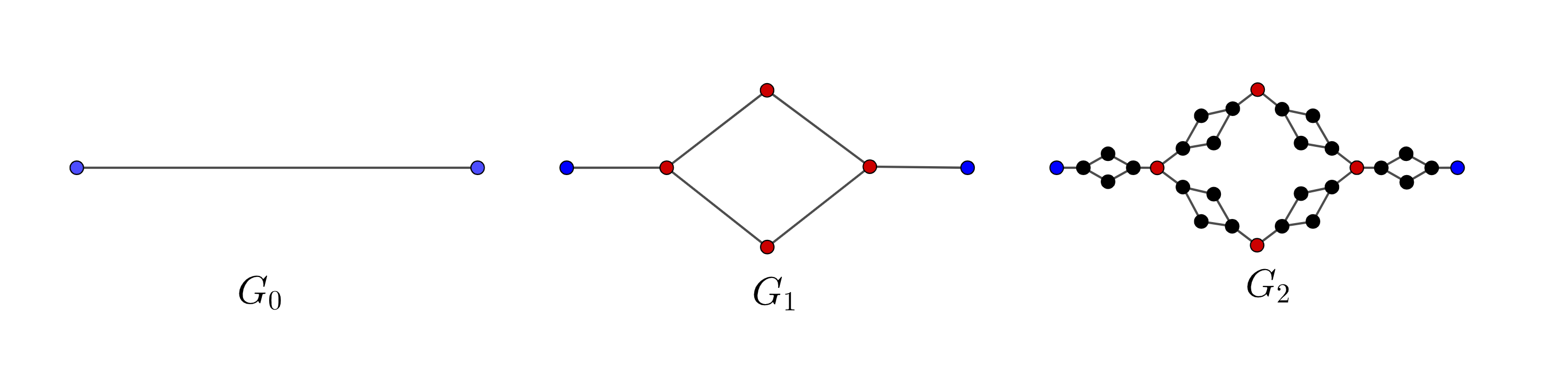
We define the Laakso graph as the inverse limit of the system
| (3.4) |
of metric graphs shown in Figure 2. For each , is equipped with the path metric so that the diameter of is equal to one. In particular, , is the metric graph indicated in Figure 2, and is obtained from by replacing each edge in by a scaled copy of with scaling factor . The projection maps are defined as follows. First, is defined by the condition that each of the two geodesic paths in from to is mapped isometrically to the directed line segment . Then is defined, on each , by conjugating the action of by . The collection (3.4) is an inverse limit system of metric graphs; see [4, Section 2.2] for an introduction to this topic. The Laakso graph is the inverse limit of the system (3.4), see [4, Section 2.4]. In particular, is equipped with a well-defined metric so that
and there exist projection maps so that . All of the maps and are -Lipschitz.
In what follows, we prove that is full. For each , we will construct an ultrametric subset with cardinality in the th approximating graph . The sets will converge in the inverse limit topology to a limit subset of infinite cardinality. Since the ultrametric property is stable under such convergence, is again ultrametric and hence provides an example of an infinite subset of satisfying the condition.
Let be a subset of cardinality obtained as for some fixed abscissa . For example, in the graph we may choose and in the graph we may choose ; see Figure 2. The branching structure of the Laakso graph induces a canonical enumeration by -tuples of binary digits. For , set . Then
| (3.5) |
where and
For instance, when we have , when we have
-
•
and
-
•
for all ,
and when we have
-
•
for all ,
-
•
for all and all , and
-
•
for all and all .
We claim that is an ultrametric space. To see this, observe that (3.5) implies that aligns with the representation of as a rooted binary tree of level . Vertices of this tree correspond to elements of (considered as initial segments of elements in ), and the distance between points and , , is . Thus is an ultrametric space.
The sequence Gromov-Hausdorff converges to [4, Proposition 2.17]. Let denote a Gromov–Hausdorff limit of the sets . Since the ultrametric condition passes to Gromov-Hausdorff limits, is ultrametric. Since , is an infinite set.
Remark 3.7.
We can obtain a larger ultrametric subset of the Laakso graph as follows. For each , we may find two isometric copies of the set defined above, whose mutual distance is at least as large as the diameter of . Thus we may choose . For instance, in the graph we may choose and ; see Figure 2. Then is again an ultrametric set. However, no ultrametric subset of can contain any three distinct points along any horizontal geodesic joining the endpoints of .
We also recall that all free spaces are doubling, as was proved by Lebedeva, Ohta, and Zolotov [24, Theorem 6].
Theorem 3.8 (Lebedeva–Ohta–Zolotov).
If there exists such that is free then is doubling.
Remark 3.9.
The converse of Theorem 3.8 is not true. In Example 3.5, if one considers the sequence for which , then one obtains a doubling metric tree containing an infinite ultrametric set. Thus is not free for any . Other examples of doubling spaces which are full for some include the Heisenberg group and the Laakso graph.
Remark 3.10.
Theorem 3.11.
For each and each -free metric space , there exist constants and and an -bi-Lipschitz embedding of into . Moreover, and depend only on the maximal cardinality of an subset of .
Taken together, Proposition 2.24 and Theorem 3.11 imply that if is either -free or satisfies the condition for some , then embeds bi-Lipschitzly into some finite-dimensional Euclidean space. While these two conditions stand at opposite extremes (one hypothesis asserts that all triplets in satisfy the condition, while the other hypothesis states that there is a fixed upper bound on the cardinality of any subset of with the condition), we do not see a path here to resolve the longstanding open problem of characterizing those metric spaces which admit finite-dimensional Euclidean bi-Lipschitz embeddings. For example, the metric trees considered in Example 3.5 are all -full and do not fall into either of the previous two categories (-free or satisfying the condition for some ). However, Proposition 3.19 shows that bi-Lipschitz embeddability and the doubling property depend on the rate of convergence of the defining sequence .
3.2. Subsets of Euclidean snowflakes
Lemma 2.10 asserts that if is a snowflaked metric space, then satisfies the condition. In general, a space satisfying the condition may not satisfy the condition for any choice of . The following theorem and its corollaries show that, in certain cases, we can ensure the existence of large (even infinite, or even of positive Hausdorff dimension) subsets of snowflaked metric spaces which verify the condition for smaller choices of .
In what follows, denotes the Euclidean metric.
Theorem 3.12.
Fix . Then there exists a sequence of real numbers so that satisfies the condition.
In fact, is a geometric sequence: for all . It follows that the set has Assouad dimension zero, and hence also has box-counting and Hausdorff dimension equal to zero.
Proof.
Given as in the statement of the theorem, set
| (3.6) |
Then , , has a unique extremum in the interval at
and
Hence has a unique maximum in the interval at , and it follows that has a unique root in the interval .
Set and for all . It suffices for us to prove that
| (3.7) |
Since is a geometric sequence, the case is easily reduced to the case via scaling. Consequently, it is enough for us to verify that
| (3.8) |
For define
Then , , and has a unique extremum at
Clearly for all , however, we have if and only if i.e.
| (3.9) |
If (3.9) holds then
and so has a unique maximum in the interval at . If (3.9) does not hold then is monotonic in with a maximum at . Regardless of whether or not (3.9) holds, we conclude that for all , in particular, for all . This establishes (3.8), and the other two statements in the definition of the condition are trivial. We therefore conclude that is an set. ∎
Now, we present some immediate corollaries of Theorem 3.12. Corollary 3.15 restates Theorem 1.2 from the introduction.
Corollary 3.13.
Let . Then is full for each .
Remark 3.14.
Observe that the conclusion fails dramatically when : the largest ultrametric set in for contains at most two points. To see this, let with , and assume without loss of generality that . If is ultrametric, then we must have
but this contradicts the fact that is an increasing function.
Corollary 3.15.
Let and let be a metric space containing a nontrivial geodesic. Then is full for each .
We now improve Theorem 3.12; instead of finding a sequence with the condition we find a subset of positive Hausdorff dimension with that property. For given , let be the unique root in of the function in (3.6), as discussed in the proof of that theorem. If , let denote the self-similar Cantor set in obtained as the invariant set for the iterated function system , . Note that the sequence defined in the proof of Theorem 3.12 is contained in . Moreover, has Hausdorff dimension .
Proposition 3.16.
Let and choose satisfying
Let be defined as above, and let be the corresponding self-similar Cantor set. Then satisfies the condition for
| (3.10) |
Moreover, and as for fixed .
Observe from (3.6) that and are related by the equation
| (3.11) |
Proof.
It suffices to prove that for any with , the inequality
holds true.
Denote by and the two self-similar pieces of . By scaling invariance, we can assume that all three points are not contained entirely in , nor are all three points contained in . In view of the ordering of these points, this means that we must have and . We will show the following two claims:
| (3.12) |
and
| (3.13) |
In fact, (3.13) follows by symmetry once we have established (3.12).
We now turn to the proof of (3.12). Our assumptions guarantee that
and our goal is to prove that
| (3.14) |
Fixing and , we first observe that the function is decreasing on . It thus suffices for us to prove that
| (3.15) |
An elementary computation gives
and
Hence for any and is maximized on . Furthermore, and for all and as for all . It follows that
It follows from (3.10), the concavity of , and the bound , that
Moreover, from (3.10) and (3.11) we find that
and hence as . ∎
It is interesting to observe that all of the examples of subsets used to illustrate the fullness of as involve geometrically convergent constructions (e.g. geometric sequences or self-similar Cantor sets). In contrast, Example 2.11, which highlights the sharpness of Lemma 2.10, involves an arithmetic sequence. The distinction between arithmetic and geometric structure can also be witnessed in the following result.
Proposition 3.17.
Let have positive Lebesgue density, and let . Then does not satisfy the condition for any .
Proof.
Let be a point of Lebesgue density for , and choose a sequence , , so that
| (3.16) |
Here we denote by the Lebesgue measure of a set . Set . For each , we claim that there exist points with
| (3.17) |
and
| (3.18) |
Indeed, if is empty, then
| (3.19) |
which contradicts (3.16). Hence there exists as in (3.17), and a similar argument assures the existence of as in (3.18). For each , the triple of points in satisfies
and
We see that the triple is asymptotically arithmetic, i.e., the arithmetic identity is approached in the limit as .
Suppose that satisfies the condition. We will show that
| (3.20) |
Applying the condition for the triple gives
whence
Letting yields (3.20) and completes the proof. ∎
To conclude this section we characterize when a snowflaked metric space isometrically embeds into an free space. In the special case when the target space is a finite-dimensional normed vector space, the following result is [23, Corollary 2.2].
Theorem 3.18.
Let be a metric space. Then there exists so that isometrically embeds into an free space if and only if is finite.
Proof.
Assume there is an such that isometrically embeds into an free.metric space . Then is also free, so there exists such that for , . Thus is finite.
Conversely, assume that is finite. By [13], there exists and there exists such that embeds isometrically in . Since is free, the conclusion follows. ∎
3.3. Bi-Lipschitz embeddability of countable ultrametric spaces with one limit point
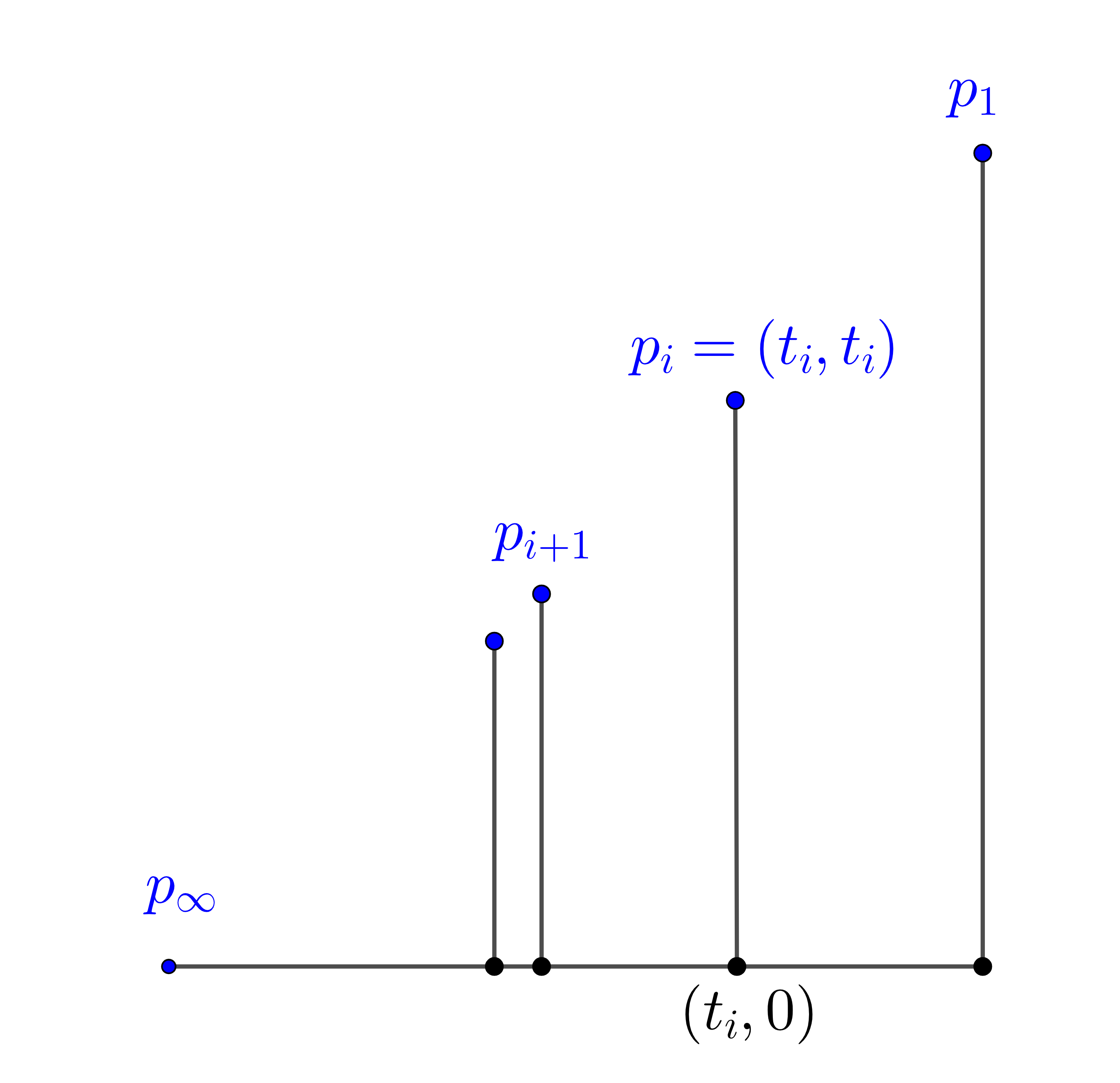
The following proposition characterizes the doubling and bi-Lipschitz embeddability properties of metric trees (as in Example 3.5). Additionally, we characterize these properties for the compact countable ultrametric spaces with a single limit point from which these trees are defined and which also satisfy condition (3.23). We begin with some notation. Let
be a compact countable ultrametric space, where and is the unique limit point of . Reordering the sequence as necessary, we may assume that the function is non-increasing.
Let be the maximal strictly decreasing subsequence of , i.e., and . Let be the metric tree associated to the sequence as in Example 3.5.
Finally, let , where for each we have . Observe that isometrically embeds into as the set of endpoints of the vertical line segments, see the discussion in Example 3.5.
Observe that if are two points so that and with , then
| (3.21) |
Indeed, since and , the ultrametric condition implies that . On the other hand, if we assume without loss of generality that , then the ultrametric condition also implies that
| (3.22) |
Since we conclude from (3.22) that and so (3.21) holds true.
Proposition 3.19.
Let be a compact countable ultrametric space with a single limit point , and let be the associated metric tree as described in the previous paragraph. Then the following are equivalent:
-
(1)
is doubling.
-
(2)
bi-Lipschitz embeds into for some .
-
(3)
There exists and such that for all .
-
(4)
.
In case any of the above conditions are satisfied, then has finite total length.
Moreover, if
| (3.23) |
then the above four conditions are also equivalent to
-
(5)
is doubling.
-
(6)
bi-Lipschitz embeds into for some .
In case these conditions on are satisfied, then is finite.
Before turning to the proof, we give an example which shows that the extra condition (3.23) is needed for the equivalence with conditions (5) and (6).
Example 3.20.
Choose an increasing sequence of integers and define a compact countable ultrametric space with metric by setting
where and setting . That is, if either or (or both) lie in ,
and so on. The space contains equilateral subsets of arbitrarily large cardinality, and hence does not bi-Lipschitz embed into any finite-dimensional Euclidean space. In particular, is not doubling. Moreover, condition (3.23) is not satisfied, since .
Proof of Proposition 3.19.
We establish this result by proving the implications in the following diagram:
| (3.24) |
and in case (3.23) is satisfied, the further implications
| (3.25) |
Note that the implications and are trivial. Moreover, the implication follows from the fact that there exists a bi-Lipschitz embedding of an ultrametric space into for some if and only if is doubling [28, Proposition 3.3].
We now show that , which we prove by contradiction. Assume that for each and there exists so that . Choose . Recall that for all . It follows that for all ,
Moreover, for all satisfying ,
Thus we found a set of points with pairwise distances at least within a ball of radius . Since was arbitrary, we conclude that is not doubling, and hence is also not doubling.
Note that the above proof also shows that , since is a subset of .
Next, we verify that . Assume that (3) is satisfied for some and , and choose so that . Then for all . Thus for each , and consequently,
Conversely, suppose that (4) is satisfied. Then . Choose so that
| (3.26) |
It follows that (3) holds true with and .
To complete the verification of the implications in (3.24), we show that . Assuming that condition (4) holds, choose as in (3.26). We define an embedding of into (equipped with the metric) as follows. Let be an orthonormal basis for . For a point with , we set
while for a point with and , we set
where is the residue of mod , i.e., for some integer .
Let and be two points lying on distinct vertical line segments in . Assume without loss of generality that . Then
| (3.27) |
If the residues of and mod are distinct, then
This holds, in particular, if .
Assume therefore that and and have the same residue mod , i.e., and . Then and hence
| (3.28) |
In this case,
| (3.29) |
It is clear from (3.27) and (3.29) that . For the converse inequality, it suffices to prove that
for some absolute constant . We will show that the conclusion holds with .
Suppose first that
| (3.30) |
Then the desired inequality is
In view of (3.30) it suffices to have
and in view of (3.28) and the fact that it suffices to have
| (3.31) |
and so the choice suffices.
Next, suppose that
| (3.32) |
Following a similar line of reasoning, we again arrive to (3.31) and conclude that suffices.
We conclude that if condition (4) holds, then defines a -bi-Lipschitz embedding of into with the metric. Hence embeds -bi-Lipschitzly into for some .
Assuming now that one of the conditions (1) – (4) is satisfied, we compute the length of the metric tree as . Since
we conclude that is rectifiable.
To finish the proof, we show that the remaining implication in (3.25) holds under the extra assumption (3.23). Thus assume that is an -bi-Lipschitz embedding, and that for all . We will construct a bi-Lipschitz embedding . Considering only the subset in we have that
In particular, if then we have
For each , the sequence contains an ultrametric subset consisting of at most elements satisfying the condition
| (3.33) |
Let be an isometric embedding; see Theorem 2.27 for the existence of such a map. Applying a translation in if necessary, we also assume that the point (which occurs as an element in ) is mapped by to the zero element of .
We now define
for , where is defined as in (3.33), and we show that this map is the desired bi-Lipschitz embedding.
Now let and be any two indexes satisfying and . If then
We thus consider the case , and we assume without loss of generality that . Then
see (3.21) for the final equality. On the other hand,
We conclude that is a bi-Lipschitz embedding of into . We leave to the reader the verification that is finite in this situation.
This completes the proof of Proposition 3.19. ∎
4. Ordered sets and rough self-contracting curves
4.1. Definitions, background and motivation
The following class of curves was studied in [7] (where the same curves were introduced but with reverse parametrization). We give a unified definition which covers both the case of curves and finite sets.
Definition 4.1 (Rough -self-contracting curve).
Fix and let be a compact subset. A map from into a metric space is said to be a rough -self-contracting curve fragment if for every in we have
| (4.1) |
We typically consider the case when the parameterizing set is either an interval (in which case we call a rough -self-contracting curve) or a finite ordered set (in which case we call a rough -self-contracting finite ordered set). We stress that is in general not assumed to be continuous.
In what follows, we shall assume that all curves are injective mappings, as a non-injective rough -self-contracting curve would necessarily be locally constant. The set inherits a total order from , defined as follows: if there exist with such that and then we write .
The case corresponds to the original notion of self-contracted curves introduced in [9], while corresponds to the class of geodesic sets, i.e., subsets of with the Euclidean metric. Inverting the orientation gives the analogous notion of rough -self-expansion, introduced in [7] under the name -curves, the case corresponding to the class of self-expanded curves. A map is rough -self-contracting if and only if given by is rough -self-expanding.
Finally, we say that is a rough -self-monotone curve if it is either rough -self-contracting or rough -self-expanding. One can also analogously define rough -self-monotone sets. Notice that the class of rough -self-monotone curve is invariant under time reversal.
Example 4.2.
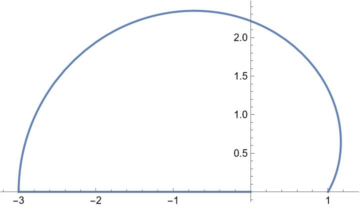
Let and be two points in and let us determine where a third point, , could be located in order that (4.1) be satisfied. For simplicity, assume , and . Then (4.1) reads
| (4.2) |
In other words, the image of under a rough -self-expanding map with and must lie in the region . Now let
see Figure 3 for the case .
The class of rough -self-monotone curves can be related to other classes of curves in the literature. For instance, let us discuss the connection to the well-known class of bounded turning curves.
Definition 4.3 (Bounded turning curves).
Let be a injective curve. We say that is -bounded turning if, for any pair of points in ,
where denotes the arc connecting to .
Lemma 4.4.
Every rough -self-monotone curve is -bounded turning for and -bounded turning for .
Proof.
Without loss of generality, we can assume that the curve is a -self-expanding curve. Let . For , the triangle inequality gives
Summing this inequality with (4.1) yields
| (4.3) |
Let . Notice that
by two applications of (4.3). To finish the proof, observe that every rough -self-expanding curve for is self-contracting so it is -bounded turning. ∎
For later purposes, we define
Observe that the converse of Lemma 4.4 does not hold. For an example with , let and let . The curve is -bounded turning but it is not self-expanding.
On the other hand, every -bounded turning curve is both self-expanding and self-contracting.
Remark 4.5.
Any compact metric space satisfying the condition (i.e., any compact ultrametric space) can be equipped with a linear order with respect to which it satisfies the -bounded turning condition, and hence is both self-expanding and self-contracting. See, e.g., [18, Lemma 2.3].
4.2. Main theorem
In what follows, we prove Theorem 1.3, which asserts the rectifiability of bounded, roughly -self-monotone curves in free metric spaces for suitable choices of and . For the reader’s convenience we restate the theorem here, along with several remarks.
Theorem 4.6.
Let and let be an free metric space. Then there exists so that any bounded, rough -self-monotone curve in , with is rectifiable. Furthermore, the length of is at most for some constant .
Remark 4.7.
We recall that Zolotov [41] proves that self-contracting curves () in free metric spaces are rectifiable whenever . It remains unclear whether this result is sharp; specifically, whether the existence of an unrectifiable self-contracting curve in necessarily implies that is not free for any . The proof which we give for Theorem 4.6 closely follows Zolotov’s argument.
Remark 4.8.
The dependence of and on the metric space is only in terms of the maximal cardinality of any subset satisfying the condition. See e.g. Remark 2.9 for estimates on the size of in the case when . When , the value of which we obtain through our proof is substantially smaller than the best currently known value (e.g. ) from [7]. However, the argument which we provide here uses only general metric properties of the underlying space, and does not rely on specifically Euclidean convex geometric results such as the Carathéodory theorem. As such it applies to a substantially broader array of ambient spaces.
Remark 4.9.
Observe that bounded unrectifiable self-monotone curves can be constructed in various spaces, including the Heisenberg group (Example 3.3), Hilbert spaces (Example 3.4), and some metric trees (Example 3.5). In Hilbert spaces, such a curve can be constructed as shown in [35, Example 3.5] or [8, Example 2.2]. Additionally, the set is a self-contracting curve, as demonstrated in [24, 8.1]. By Remark 4.5, self-monotone curves can also be constructed in metric trees or Laakso graphs, as they are full.
One can easily check that the sequence of points in Example 3.5 forms a self-contracting curve.333Here is a non-continuous self-contracting curve and its length is defined as the length of the polygonal curve connecting the points. However, the finiteness of the length of the curve depends on the defining sequence . For instance, the sequence yields a curve of infinite length, while the sequence results in a curve of finite length. See, for example [24, Example 31 and 32]. Furthermore, one can check that in the first case, does not admit a bi-Lipschitz embedding into Euclidean space, while in the second case it does. See also Proposition 3.19.
Whether or not there exists a bounded unrectifiable self-monotone curve in the Laakso graph remains an interesting open problem, see the discussion surrounding Question 5.9 for more details.
Remark 4.10.
Theorem 4.6 also applies to semi-globally free spaces. A metric space is said to be semi-globally free, for , if for each and there exists such that for each , if satisfies the condition then . The class of semi-globally free spaces (see [24, Theorem 2]) includes the following:
-
•
Finite-dimensional Alexandrov spaces of curvature with .
-
•
Complete, locally compact Busemann NPC spaces (e.g., CAT(0)-spaces) with locally extendable geodesics.
4.3. Proof of Theorem 1.3
The first step in the proof is a reduction from curves to finite ordered sets. To this end, we introduce discrete analogs for the diameter and length of a curve .
Definition 4.11 (Discrete diameter and discrete length).
Let be a finite set of real numbers, and let be a discrete ordered set, with . Define the discrete length of to be
and the discrete diameter of to be
The terminology ‘discrete diameter’ is motivated by the case of rough -self-monotone sets. Note that if is a rough -self-monotone set, then , where is defined just after the proof of Lemma 4.4.
Remark 4.12.
Note that if is a bounded, unrectifiable curve and is any positive constant, then there exists a discrete ordered subset with . Stated another way, if is bounded and for all discrete ordered subsets of , then is rectifiable and has length at most .
We now state a discrete analog of Theorem 1.3.
Theorem 4.13.
For each and , there exists and so that if is a rough -self-monotone finite ordered set, , satisfying , then contains a element subset satisfying the condition.
Proof of Theorem 1.3.
Assume that is an free metric space, and fix an integer so that contains no subset of cardinality . Choose as in the statement of Theorem 4.13 and assume that is a bounded and unrectifiable rough -self-monotone curve for some . Observe that if a rough -self-monotone curve consists of a finite set of points, it is trivially rectifiable. Thus, without loss of generality, we may assume that the curve contains an infinite set of points. Let be the constant guaranteed by Theorem 4.13. Since is bounded and unrectifiable, we can choose a finite ordered set so that . Then contains an subset of cardinality , but this contradicts the choice of .
We now turn to the proof of the final claim of the theorem. Assume that is a bounded and rectifiable rough -self-monotone curve with where is as above. Then contains no subset satisfying the condition of cardinality . It follows that
for every rough -self-expanding finite ordered subset . By Remark 4.12, the length of is at most . ∎
Remark 4.14.
Note that the parameter depends on the metric space . In (2.2), a bound for in the Euclidean case is given.
We now discuss the relationship between the rough self-expanding and contracting conditions and the condition in the setting of a finite ordered set . Recall that the former conditions impose two restrictions on the mutual distances between three points, stated relative to the given ordering on . In contrast, the condition imposes restrictions on the mutual distances between three points in , which must hold with respect to any permutation of the points. More precisely, if are points in , then the rough -self-expanding condition asserts that
while the rough -self-contracting condition asserts that
On the other hand, in order to check the condition for this particular triple of points, we must verify all of the following inequalities:
We assume that . In order to derive the conclusion for such a triple, selected from a set which is both rough -self-expanding and -self-contracting, it suffices to verify that either
| (4.4) |
or
| (4.5) |
holds true. To simplify matters we work consistently with (4.4).
Definition 4.15.
A finite ordered set in a metric space is said to satisfy the medial ordered condition if the inequality (4.4) holds true for any choice of in .
We record an elementary lemma which formalizes the preceding discussion.
Lemma 4.16.
If is a finite ordered set which is both rough -self-expanding and -self-contracting and which satisfies the medial ordered condition, then satisfies the condition.
We will reduce the proof of Theorem 4.13 to the following two technical propositions.
Proposition 4.17.
Let and . Then there exist and so that if is a finite, ordered, rough -self-monotone set, , with , then and there exists so that satisfies the medial ordered condition.
Proposition 4.18.
Let and let . If
| (4.6) |
then there exists an integer so that if , , is a finite, ordered, -bounded turning set satisfying the medial ordered condition, then
| (4.7) |
for some , .
We now show how to derive Theorem 4.13 as a consequence of Propositions 4.17 and 4.18. From now on, without loss of generality, we assume that our curve or set is roughly -self-expanding. The proof makes use of Ramsey’s theorem for -uniform hypergraphs. The relevant Ramsey number is the least integer such that for any -coloring of the set of all unordered triples of elements in a set of elements, there exists either a subset of of size such that all unordered triples formed by elements of are monochromatic in the first color, or a subset of of size such that all unordered triples formed by elements of are monochromatic in the second color.
The upper bound
| (4.8) |
where is an absolute constant, is due to Conlon–Fox–Sudakov [5], see also Sudakov’s 2010 ICM proceedings article [36]. For our purposes, it is enough to know that is finite, although we do make use of (4.8) to give an explicit upper bound for the parameter in Theorem 1.3.
Proof of Theorem 4.13.
Let and be given. The value will satisfy several constraints, the first of which is
| (4.9) |
See also (4.10). We note that (4.9) is equivalent to
If is a rough -self-expanding set with , then is -bounded turning with as in Lemma 4.4. Moreover,
Furthermore,
and
since . Choose with so that
Choose an integer as in Proposition 4.18. Since both and here have been chosen to depend only on , we have .
We next appeal to the two parameter Ramsey’s theorem for -uniform hypergraphs, and choose an integer so that if the collection of all triples in is -colored, then either there exists a subset of cardinality so that all triples in are colored red, or there exists a subset of cardinality so that all triples in are colored blue. By (4.8),
for some absolute constant .
By Proposition 4.17, choose constants and so that the stated conclusion holds true. In the statement of that proposition, and depend on and ; tracing the dependence above we see that in the context of this proof we have and eventually depend on and . We impose the second assumption
| (4.10) |
and we assume that a choice of has been made so that both (4.9) and (4.10) are satisfied.
Assume now that is a rough -self-expanding finite ordered set of cardinality so that . Proposition 4.17 implies that and we may choose a subset of cardinality so that satisfies the medial ordered condition. We identify with the index set and we color the set of all triples as follows:
-
•
Triple is colored red if .
-
•
Triple is colored blue if .
Since is rough -self-expanding and , is -bounded turning. The Ramsey-type conclusion above tells us that one of the following statements is valid:
-
(i)
There exists a subset of of cardinality in which all triples are colored red.
-
(ii)
There exists a subset of of cardinality in which all triples are colored blue.
Observe that if (ii) is satisfied, then we have found a element subset of which is a bounded turning set, satisfies the medial ordered condition, and for which the inequality holds for all . This contradicts the conclusion which we obtain from Proposition 4.18, namely, that for any subset of of cardinality there exists an index so that (4.7) holds.
Hence (i) must be satisfied. Let with have the property that all triples in are colored red. Then
-
•
is rough -self-expanding (since is rough -self-expanding and ),
-
•
satisfies the medial ordered condition (since ), and
-
•
is rough -self-contracting (since all triples in are colored red).
By Lemma 4.16, satisfies the condition. ∎
It remains to verify the two technical propositions.
Proof of Proposition 4.18.
Fix , , and as in the statement. Assume that is a finite, ordered, -bounded turning set satisfying the medial ordered condition, and write . We argue by contradiction, so assume that for every choice of , , the inequality
| (4.11) |
holds true. We will find an upper bound for depending on the data .
The -bounded turning condition implies that . By induction, and using the medial ordered condition, we deduce that
| (4.12) |
Summing (4.11) over this range of indexes gives
and hence
Thus
and so
We conclude that
where the upper bound depends only on , , and . ∎
Finally, we turn to the proof of Proposition 4.17. This proof is long and technical, and we will break the argument into intermediate steps which will be formulated as individual lemmas. The overall structure of the proof is by contradiction. Assuming that the conclusion does not hold, we define inductively a sequence of -point subsets of for which the -tuples of indexing integers are coordinate-wise non-decreasing. By assumption, the stated conclusion does not hold at any stage of this construction. We continue until the final (th) entry of the sequence is sufficiently close to . Along the way we introduce a suitable weighted sum of entries, which we show to be roughly non-decreasing with respect to the inductive parameter. Once the process stops, we compare the resulting quantity with the discrete length and diameter of the original set, and observe that the estimate which we obtain is incompatible with the initial assumption that , provided is sufficiently large. This yields the desired contradiction, and thereby completes the proof of the proposition.
Proof of Proposition 4.17.
We will prove the result by contradiction, and the necessary constants and will be determined at the conclusion of the proof, see (4.20) and (4.21). Let be a finite, ordered, rough -self-expanding set with and . We first show that if the constant is chosen sufficiently large (in terms of and ), then . Indeed, using the -bounded turning property of , we find that for each . Hence
Provided we choose
| (4.13) |
it follows that as desired. Note that the actual choice of which we make in (4.21) satisfies (4.13). Moreover, the value for which we determine in (4.20) satisfies , whence
| (4.14) |
We now start the proof by contradiction, and we suppose that every -element subset fails to satisfy the medial ordered condition. For each such subset , choose indexes from the set so that
| (4.15) |
We define inductively a sequence of -element subsets of . For each , let be the corresponding subset of , i.e., .
Remark 4.19.
The number of subsets in the sequence which we will define is on the order of , see Remark 4.20. As a result, we need to make sure as the proof continues that our eventual choice of the comparison constant does not depend on .
First, we set
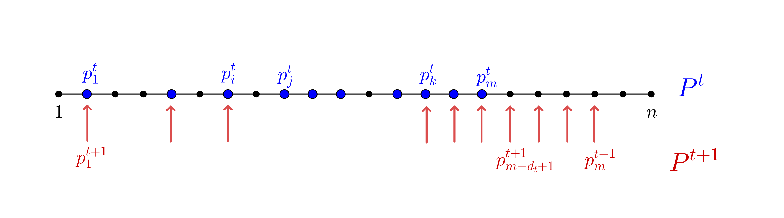
Next, assume that has been defined, with . Choose indexes
satisfying
The successor set will be defined by removing all elements of between and and adding in an equal number of elements immediately to the right of . More precisely, let
We consider two cases.
-
Case 1:
. In this case we stop the inductive process, and we set .
-
Case 2:
. In this case, we set
See Figure 4 for a graphical visualization of this process.
Remark 4.20.
It is clear from the construction that the sequence is nondecreasing for each . Moreover, for all choices of we have , whence
Since for all we conclude that . On the other hand, the termination condition (Case 1) is . Hence or .
Next, we fix the weighting factor
| (4.16) |
where the coefficient has been determined by the bound in (4.14).
For each , define the following weighted sum:
The sum in question is taken over two parameters and satisfying . In what follows, we omit the explicit reference to the pair in later instances of such sums.
Lemma 4.21.
For each ,
| (4.17) |
for some constant .
Assuming temporarily that Lemma 4.21 is true, we complete the proof of the proposition. Summing (4.17) from to yields
Considering only terms with and dropping all powers of the weighting factor , we have
Thus
or equivalently,
By Lemma 4.4, is -bounded turning. Hence for all , and so
For each such and , we have by the triangle inequality. Thus
and we conclude that
Finally, we estimate the term . Using the bounded turning property again, we find
The quantity can be explicitly computed as a function of and , alternatively, we can use the trivial upper bound
| (4.18) |
Using (4.18) for simplicity, we obtain
and therefore
| (4.19) |
provided . (Here we again used (4.14)). The bound in (4.19) tells us how to choose the constants and in the statement of Proposition 4.17. To wit, set
| (4.20) |
and
| (4.21) |
∎
Proof of Lemma 4.21.
We break into three separate terms, as follows:
| (4.22) |
Lemma 4.22.
If the index is chosen so that , then
Lemma 4.23.
If the index is chosen so that , then
Lemma 4.24.
Postponing the proofs of these three lemmas, we complete the proof of Lemma 4.21. Summing the estimates for , , and from the three lemmas, we obtain
| (4.23) |
where
and
Recall that the indexes and were chosen so that and .
We now show that and one of the following two conclusions holds true:
-
•
and , or
-
•
and .
Using these bounds in (4.23) we derive the desired conclusion
and thus complete the proof of Lemma 4.21.
We first analyze the remainder term . Since , it follows that whenever . In particular, since we have . It follows that
and
and hence
In view of the choice of in (4.16), we conclude that .
We analyze the remainder terms and simultaneously, dividing into two cases:
-
(i)
, and
-
(ii)
.
We start with case (i). Note that by construction, if , then . Moreover, each of the pairs with occurs as a pair of the form for some with . Thus
Furthermore, , and so whenever . Thus
and hence
We conclude that if
| (4.24) |
but note that (4.24) is satisfied if is chosen as in (4.16), since .
Alternatively, assume that case (ii) holds. In this case,
Also, if , then , and each of the pairs with occurs as a pair of the form for some with . Thus
This finishes the proof of Lemma 4.21. ∎
Proof of Lemma 4.22.
Recall that we fix so that , and we consider the sum of terms in over pairs so that . For such and , we necessarily have and by construction. If we also fix so that , then .
For each pair so that , the rough -self-expanding condition implies that
| (4.25) |
For the particular choice , we have the following alternate inequality which follows from (4.15):
| (4.26) |
Summing over all for which , we conclude that
To complete the proof of this lemma, we estimate
where
and is chosen as in (4.16). ∎
Proof of Lemma 4.23.
Since we chose so that , in this case we restrict to the sum of terms in over pairs with . Our goal is to estimate
In this case, we have by construction. Moreover,
| (4.27) |
For with we use the triangle inequality to get
| (4.28) |
while for with we use the -bounded turning property to get
| (4.29) |
Thus
Due to (4.27),
Combining all of the above yields
as desired. ∎
Proof of Lemma 4.24.
In this final case, we consider pairs with . If then and so
by the bounded turning condition. On the other hand, if then
It follows that
as desired. ∎
5. Questions and further comments
In this section we collect several open problems motivated by our work, along with some relevant discussion and further comments.
Question 5.1.
For a given metric space , compute
| (5.1) |
If no such value exists, we set . Recall that -self monotone curves in any metric space are just geodesics, and hence are always rectifiable.
By results in [7], we have for every . Our main theorem (Theorem 1.3) states that whenever is free for some . By results discussed earlier in this paper, we have that when is the sub-Riemannian Heisenberg group, or Hilbert space, or Laakso space, or the metric graphs considered in Example 3.5.
We do not know any examples of free metric spaces for which , so it could be true that the value in (5.1) for such spaces is always equal to one.
In connection with the previous discussion about the possible freeness of the Heisenberg group, we pose the following question.
Question 5.2.
Is the first Heisenberg group equipped with the Carnot–Carathéodory metric free? If so, what is the largest size of an ultrametric subset of ?
In [19], the equilateral dimension of a metric space is defined to be the cardinality of the largest equilateral subset of , where a subset is said to be equilateral if there exists so that for all distinct in . Clearly, every equilateral subset is an ultrametric subset. The equilateral dimension of in the Euclidean metric is , and equilateral dimensions of other finite dimensional normed vector spaces are known. See [19] for a review of these results. In [19], the authors show that the equilateral dimension of is , where denotes the Korányi metric on the Heisenberg group . However, it is not clear how to extend their argument to study Question 5.2.
The study of self-contracting curves in Euclidean space was heavily motivated by applications to gradient flows for convex functions. This connection has been worked out in detail in Euclidean and Riemannian spaces, but to the best of our knowledge the following possible extension has not been considered.
Question 5.3.
Are the integral curves associated to the horizontal gradient flow of an H-convex function in a domain of the Heisenberg group necessarily self-contracting, in either the Korányi metric or the CC metric ?
Regarding roughly self-contracting curves, the following question also remains open, even in Euclidean space.
Question 5.4.
Do roughly self-contracting curves arise as integral curves associated to a gradient flow? If so, what is the relevant class of functions whose gradient flows generate such curves?
Finally, we collect a few additional questions of a more technical nature, which arise in connection with specific remarks or examples in this paper.
Question 5.5.
Let and . Does there exist a set so that satisfies the condition, but fails to be a metric space for any ?
Question 5.6.
For which values does there exist a set in which is , yet fails to be a metric space for any ?
Recall that in Example 2.12 we saw that metric spaces with the above property exist for any , however, the examples constructed there did not admit any obvious embedding into any uniformly convex Banach space. For subsets of Hilbert space the best example we currently have is given in section 7, and only valid for .
Question 5.7.
Does there exist any value for which the conclusion in Theorem 1.3 holds true for any metric space?
Question 5.8.
If a metric space contains a bounded, unrectifiable self-monotone curve, must be full for some choice of ?
Question 5.9.
Does the Laakso graph contain a bounded, self-contracted, unrectifiable set?
Recall that in Example 3.6 we constructed an infinite ultrametric subset as a vertical slice of . As noted before, may be equipped with a self-contracted ordering, but we do not know whether such an ordering exists which makes unrectifiable. There is, however, a self-contracted rectifiable ordering of . Such ordering may be constructed as the limit of a consistent sequence of self-contracted orderings of the finite sets , with a uniform upper bound on length. The set can be identified with the vertices of the cube , and a suitable self-contracted ordering can be obtained from a Hamiltonian cycle on the associated graph. Using the formula (3.5) for the metric on , one computes that the length of in this ordering is bounded above by , uniformly in . Details are left to the reader.
As noted in Remark 3.7, the Laakso graph contains larger ultrametric subsets, which in turn can be equipped with self-contracted orderings. However, we do not know whether any such ordering is unrectifiable.
6. Appendix A: A doubling metric space which is neither -free nor -full
The following example was provided to the authors by Tuomas Hytönen [16]. We are grateful to him for permission to include it in this paper.
Let
be the standard dyadic ultrametric on , where
are the dyadic subintervals of of length .
For each , let
Note that , and hence . We claim that each is a metric. It suffices to verify the triangle inequality . If , then
If , then
where in we used the fact that the larger of the values , , satisfies and hence .
On , let
and
where is the Lebesgue measure.
We next claim that is a doubling metric space. For the proof, we introduce the notation , for and , to denote the unique element of which contains . With this notation in place, and with a reminder that we denote by the closed ball in a metric space with center and radius , we invite the reader to verify that
It follows that there exist constants so that for all and all . Hence is an Ahlfors -regular measure on , which implies that is doubling.
The metric space contains arbitrarily large ultrametric subsets, since for each the set is an ultrametric set of size . Thus is not -free for any . On the other hand, for any such , all subsets of are finite. Indeed, suppose that is an infinite subset of , and write
If has more than points, then one of the intervals must contain at least three points of . But the restriction of to , and hence to is the Euclidean distance. Then the three collinear points of this set contradict the condition. It follows that each has at most finitely many points, in which case there must be infinitely many with . Let , , and be three such integers , and let be a point in for . Then the restriction of to agrees with the Euclidean distance on the three-point set , and this again contradicts the property. We conclude that does not contain any infinite set, so is not -full.
7. Appendix B: A partial answer to Question 5.6
For each , we provide an example of a subset with the property that satisfies the condition, but fails to be a metric space for any .
Fix any sequence with and . Let be a large parameter (whose value will be specified later). We define a set as follows:
Here denotes the standard orthonormal basis of , and is a unit vector in selected so that the triangle with vertices , , and has sides of length , , and .
Denote by the norm and by the metric. The proof that fails to be a metric space for any is exactly the same as in Example 2.12. It suffices for us to show that satisfies the condition.
First, we provide an estimate for the distances between points in the case when and lie in distinct two-dimensional subspaces. Let and , where . Then
| (7.1) |
Now let be distinct points in . Assume that , , and .
Step 1. If then form the vertices of a triangle in with side lengths as above, and hence the condition is satisfied.
Step 2. Suppose next that , , and are all distinct. We impose the restriction
| (7.2) |
Then and hence, using (7.1),
and the corresponding statements for all permutations of the elements , , and also hold true. Hence in this case the condition is satisfied.
Step 3. Finally, we consider the case when . Thus and . We need to verify the following three inequalities:
| (7.3) |
| (7.4) |
and
| (7.5) |
Note, however, that (7.4) and (7.5) are symmetric from the point of view of the assumptions on the points , , and . We will in fact prove that
| (7.6) |
To verify (7.3) we observe that since both and lie in . On the other hand, by (7.1). Thus (7.3) holds provided
| (7.7) |
We impose the restriction
| (7.8) |
which implies that (7.7) holds true.
Finally, we turn to the proof of (7.6). For convenience, we use an alternate representation for the points . Write , , and . Here for ; this boolean variable indicates whether or . The variable for takes on one of the following values: if and if . With this notation in place we compute
, and
If then and the desired equation (7.6) reads
| (7.9) |
Using the expressions for and above, along with the identity , we rewrite (7.9) as
| (7.10) |
Note that for and for . Indeed, if the boolean indicator this is trivial, while if then either the two components of the inner product are orthogonal and again the result is trivial, or the expression in question is bounded above by or . Hence (7.10) is implied by
| (7.11) |
Inequality (7.11) in turn is implied by
which is equivalent to
| (7.12) |
If then and we wish to verify
| (7.13) |
which we rewrite as
| (7.14) |
Using the bounds for and as discussed above, we see that (LABEL:eq:abc5) is implied by
which in turn is implied by
which is equivalent to
| (7.15) |
Finally, if then and we wish to verify
| (7.16) |
which we rewrite as
| (7.17) |
Following the line of reasoning as in previous cases, we see that (LABEL:eq:abc7) is implied by
which in turn is implied by
which is equivalent to
| (7.18) |
If we assume that the parameter is chosen so large that (7.2), (7.8), (7.12), (7.15) and (7.18) are satisfied, then we have that satisfies the condition. (Note that the restriction is necessary in order to ensure the existence of a value satisfying (7.15) and (7.18).) This finishes the proof of this example.
References
- [1] Ambrosio, L., Gigli, N., and Savaré, G. Gradient flows in metric spaces and in the space of probability measures, second ed. Lectures in Mathematics ETH Zürich. Birkhäuser Verlag, Basel, 2008.
- [2] Aschbacher, M., Baldi, P., Baum, E. B., and Wilson, R. M. Embeddings of ultrametric spaces in finite-dimensional structures. SIAM J. Algebraic Discrete Methods 8, 4 (1987), 564–577.
- [3] Assouad, P. Plongements lipschitziens dans . Bull. Soc. Math. France 111, 4 (1983), 429–448.
- [4] Cheeger, J., and Kleiner, B. Inverse limit spaces satisfying a Poincaré inequality. Anal. Geom. Metr. Spaces 3, 1 (2015), 15–39.
- [5] Conlon, D., Fox, J., and Sudakov, B. Hypergraph Ramsey numbers. J. Amer. Math. Soc. 23, 1 (2010), 247–266.
- [6] Daniilidis, A., David, G., Durand-Cartagena, E., and Lemenant, A. Rectifiability of self-contracted curves in the Euclidean space and applications. J. Geom. Anal. 25, 2 (2015), 1211–1239.
- [7] Daniilidis, A., Deville, R., and Durand-Cartagena, E. Metric and geometric relaxations of self-contracted curves. J. Optim. Theory Appl. 182, 1 (2019), 81–109.
- [8] Daniilidis, A., Deville, R., Durand-Cartagena, E., and Rifford, L. Self-contracted curves in Riemannian manifolds. J. Math. Anal. Appl. 457, 2 (2018), 1333–1352.
- [9] Daniilidis, A., Ley, O., and Sabourau, S. Asymptotic behaviour of self-contracted planar curves and gradient orbits of convex functions. J. Math. Pures Appl. (9) 94, 2 (2010), 183–199.
- [10] David, G., and Semmes, S. Fractured Fractals and Broken Dreams: Self-Similar Geometry through Metric and Measure. Oxford Science Publications, Oxford, UK, 1997.
- [11] David, G., and Snipes, M. A non-probabilistic proof of the Assouad embedding theorem with bounds on the dimension. Anal. Geom. Metr. Spaces 1 (2013), 36–41.
- [12] David, G. C., and Schul, R. The analyst’s traveling salesman theorem in graph inverse limits. Ann. Acad. Sci. Fenn. Math. 42, 2 (2017), 649–692.
- [13] Deza, M., and Maehara, H. Metric transforms and Euclidean embeddings. Trans. Amer. Math. Soc. 317, 2 (1990), 661–671.
- [14] Erdős, P., and Füredi, Z. The greatest angle among points in the -dimensional Euclidean space. In Combinatorial mathematics (Marseille-Luminy, 1981), vol. 75 of North-Holland Math. Stud. North-Holland, Amsterdam, 1983, pp. 275–283.
- [15] Gupta, A., Newman, I., Rabinovich, Y., and Sinclair, A. Cuts, trees and -embeddings of graphs. Combinatorica 24, 2 (2004), 233–269.
- [16] Hytönen, T. personal communication.
- [17] Käenmäki, A., and Suomala, V. Nonsymmetric conical upper density and -porosity. Trans. Amer. Math. Soc. 363, 3 (2011), 1183–1195.
- [18] Keleti, T., Máthé, A., and Zindulka, O. Hausdorff dimension of metric spaces and Lipschitz maps onto cubes. Int. Math. Res. Not. IMRN, 2 (2014), 289–302.
- [19] Kim, J., and Platis, I. D. Equilateral dimension of the Heisenberg group. Geom. Dedicata 217, 4 (2023), Paper No. 64, 17.
- [20] Laakso, T. J. Ahlfors -regular spaces with arbitrary admitting weak Poincaré inequality. Geom. Funct. Anal. 10, 1 (2000), 111–123.
- [21] Laakso, T. J. Plane with -weighted metric not bi-Lipschitz embeddable to . Bull. London Math. Soc. 34, 6 (2002), 667–676.
- [22] Lang, U., and Plaut, C. Bilipschitz embeddings of metric spaces into space forms. Geom. Dedicata 87, 1-3 (2001), 285–307.
- [23] Le Donne, E., Rajala, T., and Walsberg, E. Isometric embeddings of snowflakes into finite-dimensional Banach spaces. Proc. Amer. Math. Soc. 146, 2 (2018), 685–693.
- [24] Lebedeva, N., Ohta, S.-i., and Zolotov, V. Self-contracted curves in spaces with weak lower curvature bound. Int. Math. Res. Not. IMRN, 11 (2021), 8623–8656.
- [25] Lee, J. R., Mendel, M., and Naor, A. Metric structures in : dimension, snowflakes, and average distortion. European J. Combin. 26, 8 (2005), 1180–1190.
- [26] Lemenant, A. Rectifiability of non-Euclidean planar self-contracted curves. Confluentes Math. 8, 2 (2016), 23–38.
- [27] Lemin, A. Y. Isometric imbedding of isosceles (non-Archimedean) spaces into Euclidean ones. Dokl. Akad. Nauk SSSR 285, 3 (1985), 558–562.
- [28] Luukkainen, J., and Movahedi-Lankarani, H. Minimal bi-Lipschitz embedding dimension of ultrametric spaces. Fund. Math. 144, 2 (1994), 181–193.
- [29] Manselli, P., and Pucci, C. Maximum length of steepest descent curves for quasi-convex functions. Geom. Dedicata 38 (1991), 211–227.
- [30] Naor, A., and Neiman, O. Assouad’s theorem with dimension independent of the snowflaking. Rev. Mat. Iberoam. 28, 4 (2012), 1123–1142.
- [31] Naor, A., Peres, Y., Schramm, O., and Sheffield, S. Markov chains in smooth Banach spaces and Gromov-hyperbolic metric spaces. Duke Math. J. 134, 1 (2006), 165–197.
- [32] Ohta, S. I. Self-contracted curves in CAT(0)-spaces and their rectifiability. J. Geom. Anal. 30, 1 (2020), 936–967.
- [33] Ryoo, S.-Y. Embedding snowflakes of Carnot groups into bounded dimensional Euclidean spaces with optimal distortion. Anal. PDE 15, 8 (2022), 1933–1990.
- [34] Semmes, S. On the nonexistence of bilipschitz parameterizations and geometric problems about -weights. Rev. Mat. Iberoam. 12, 2 (1996), 337–410.
- [35] Stepanov, E., and Teplitskaya, Y. Self-contracted curves have finite length. J. Lond. Math. 96, 2 (2017), 455–481.
- [36] Sudakov, B. Recent developments in extremal combinatorics: Ramsey and Turán type problems. In Proceedings of the International Congress of Mathematicians. Volume IV (2010), Hindustan Book Agency, New Delhi, pp. 2579–2606.
- [37] Tao, T. Embedding the Heisenberg group into a bounded-dimensional Euclidean space with optimal distortion. Rev. Mat. Iberoam. 37, 1 (2021), 1–44.
- [38] Tyson, J. T. Bi-Lipschitz embeddings of hyperspaces of compact sets. Fund. Math. 187, 3 (2005), 229–254.
- [39] Tyson, J. T., and Wu, J.-M. Characterizations of snowflake metric spaces. Ann. Acad. Sci. Fenn. Math. 30, 2 (2005), 313–336.
- [40] Zolotov, V. Bi-Lipschitz embeddings of SRA-free spaces into Euclidean spaces. arxiv:1906.02477 (2019).
- [41] Zolotov, V. Sets with small angles in self-contracted curves. arXiv:1804.00234 (2018).