A metrological framework for uncertainty evaluation in machine learning classification models

Abstract

Machine learning (ML) classification models are increasingly being used in a wide range of applications where it is important that predictions are accompanied by uncertainties, including in climate and earth observation, medical diagnosis and bioaerosol monitoring. The output of an ML classification model is a type of categorical variable known as a nominal property in the International Vocabulary of Metrology (VIM). However, concepts related to uncertainty evaluation for nominal properties are not defined in the VIM, nor is such evaluation addressed by the Guide to the Expression of Uncertainty in Measurement (GUM). In this paper we propose a metrological conceptual uncertainty evaluation framework for ML classification, and illustrate its use in the context of two applications that exemplify the issues and have significant societal impact, namely, climate and earth observation and medical diagnosis. Our framework would enable an extension of the VIM and GUM to uncertainty for nominal properties, which would make both applicable to ML classification models.

1 Introduction

1.1 Machine learning classification in metrology

The use of machine learning (ML) models offers the potential to bring great benefits to a wide range of societal challenges, for example in climate and earth observation, health care, and advanced manufacturing. ML models can be used to make sense of large data sets and learn complex relationships within them, and also to automate manual processes that require considerable time or expertise.

Many of these applications involve the measurement of some signal on an instrument and inferring information of value to society from that signal. Traditionally, such problems would have involved developing a physical or empirical model that would relate the measurements to the information of interest. Where the information of interest is a quantity or set of quantities, the empirical model developed would form what is considered in metrology a measurement model, providing the relationship between input quantities and a measurand, the “quantity intended to be measured” [1].

ML methods, and in particular, a type of ML known as supervised learning, where empirical models are built to infer predictions of a specific variable given knowledge of other variables, are increasingly being used to establish (define and parametrise) such models. The phrase “to learn the model” is commonly used in ML to describe model development using supervised learning.

The distinctive feature of supervised learning models is that they are learned from training data, rather than purely using physical intuition or laws. Two types of supervised learning are often distinguished: regression and classification. The distinction is based on the type of variable that is being predicted: a regression model predicts a quantitative variable, while a classification model predicts a categorical variable. In Section 2 we define the terms quantitative and categorical more precisely and provide examples of each.

Both regression and classification models have wide application, but the focus of this paper is on classification models. By a classification model we mean a function $f$, which takes some number of input variables and returns a categorical output variable. Formally speaking, we can denote a collection of input variables by $X$. A collection is like a vector but can include both quantitative and categorical variables. The output categorical variable is denoted by $Y$, and can be one of $K$ classes denoted by $\{c_{1},\dots,c_{K}\}$. Following the convention of the Guide to the Expression of Uncertainty in Measurement (GUM) [2], we describe an instance of these variables, that is the specific implementation given a set of measured or otherwise estimated input variables, using lower case. Thus $x$ is an instance of $X$ and $y$ is an instance of $Y$ and these are related through

$$y=f(x),\quad y\in\mathcal{C}_{K}:=\{c_{1},\dots,c_{K}\}.$$ (1.1)

In reality, most classification models output a particular type of categorical variable known as a nominal variable (sometimes referred to as an unordered categorical variable), or a nominal property in the language of the International Vocabulary of Metrology (VIM) [1], in which the categories have no natural ordering. See Section 2 for a more detailed discussion of variable types and how they are categorised in the VIM.

More specifically, an ML classification model is one that has been learned from labelled training data, by which we mean $N$ samples (or observations) of paired data $(x_{i},y_{i}),\,i=1,\dots,N$, consisting of observations of both the collection of input variables $X$ and the output variable $Y$. Any implementation of supervised learning consists of two stages: a training phase and a prediction phase. In the training phase, the model $f$ is learned from known paired inputs and outputs, which typically involves optimising the parameters of the model. In the prediction phase, the model is then evaluated upon new input variables.

1.2 Uncertainty evaluation for machine learning classification

ML classification models are currently being used in several applications in which it is crucial that predictions are accompanied by an evaluation of uncertainty. Examples include earth observation such as land cover classification, mapping of water, ice extent and cloud masking [3, 4, 5], environmental monitoring such as bioaerosol classification [6, 7], and medical diagnosis such as the detection of heart arrythmias from electrocardiogram (ECG) and photoplethysmography (PPG) signals [8, 9]. See Section 4 where we illustrate the conceptual contributions of this paper in the context of two case studies: land cover classification and atrial fibrillation detection. The importance of uncertainty evaluation for ML was highlighted in the recent Strategic Research Agenda developed by the European Metrology Network for Mathematics and Statistics (MATHMET) [10, Section 3].

In a metrology context, the outputs of an ML model may also be used to make inferences about other variables, that is, they can be used as input quantities for further measurement models or classification models. It follows that, as well as being important as an end in itself, uncertainty evaluation also enables the outputs of ML models to be used as part of an ongoing traceability chain, where the term traceability chain is used to include both traditional metrological traceability chains, where artefacts or reference materials are passed between facilities, and situations where data are passed through multiple processing steps (e.g. [11]). In Section 3.3, we provide an illustration of how the outputs of an ML classification model, along with their accompanying uncertainties, can be included as inputs to other models.

1.2.1 The uncertainty evaluation task for machine learning classification models

For classification models, a natural way to evaluate uncertainty is to assign a probability to each of the $K$ possible classes rather than simply returning a single predicted class [1, Definition 2.9]. Assigning a probability to each class of a nominal property is equivalent to obtaining the probability mass function (PMF) for the classification. In Section 3 we develop the observation that the role of the PMF here is the natural counterpart of the role of the probability density function (PDF) in the measurement of a quantitative variable (quantity). We also show in Section 3 how the PMF of a categorical variable can be used as an input into other models, allowing the propagation of uncertainty as part of the traceability chain.

Section 1.1 described how ML classification is a type of supervised learning where a model is learned that relates outputs to inputs, and where an implementation of ML classification involves a training phase followed by a prediction phase. In ML classification models, contributions to the overall uncertainty of a prediction are introduced in both the training and prediction phases, which is in contrast to rule-based classifiers in which there is no training phase.

We next outline some of the factors contributing to prediction uncertainty throughout the ML pipeline. These contributory factors are also illustrated in Figure 1.

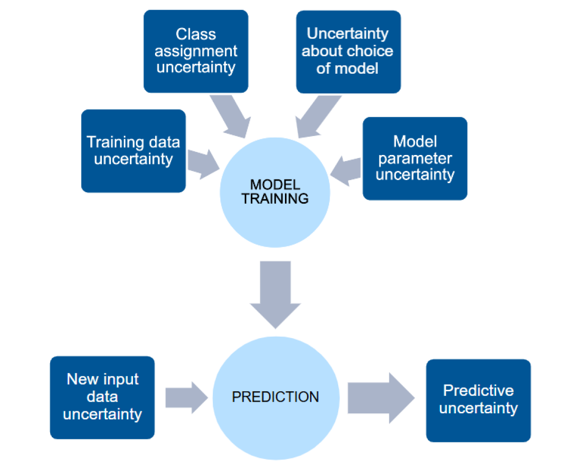
Figure 1: Factors contributing to uncertainty in ML prediction.

1. Training data uncertainty. In the training phase, one contribution to prediction uncertainty is measurement uncertainty in the training data itself. For example, when classifying landcover based upon surface reflectance measurements (see our case study in Section 4.1), there is uncertainty in the surface reflectance measurements due to imperfect knowledge of aerosol optical depth (input variables), and the landcover data is also subject to labelling errors (output data). These training data uncertainties affect the training of the model.

2. Class assignment uncertainty. In classification tasks for which ML might be used, there is typically no theoretical justification for the choice of input variables, and therefore no reason to assume that observations of the input variables are sufficient to determine a classification unambiguously. Such tasks are in this sense ill-posed: a given observation for the input variables could occur for data drawn from more than one class. In such cases, there is a limitation, inherent in the modelling task, to determining the class to which a data sample belongs. This limitation is itself dependent upon the choice of input variables. Feature selection refers to the common practice in ML of choosing a subset of available input variables, which can help to remove redundant/unnecessary input variables. However, feature selection cannot eliminate class asignment uncertainty if the original selection of variables is insufficient.

3. Uncertainty about choice of model. The supervised learning approach relies upon the selection of a certain kind of classification model, and this choice introduces uncertainty. When multiple models are compared, the “best” model is usually selected according to empirical performance, and the reliance upon empirical testing also introduces uncertainty.

4. Model parameter uncertainty. ML models need to be optimised using the training data, for example, optimising the values of its parameters. There is, therefore, also uncertainty related to the estimates of the ML model parameters. Some of this uncertainty may be due to the challenges of optimising a model with multiple local optima. The ability to optimise an ML model also depends upon having training data that provides sufficient coverage of the region of data space that is of interest. Training data requirements vary depending upon the complexity of the classification task and the chosen ML model.

5. New input data uncertainty. In the prediction phase, additional uncertainty is introduced through measurement uncertainties in previously unused (non-training) input data to which the model is being applied.

Uncertainty source (2) can be understood as inherent to the learning task. Uncertainty sources (1) and (5) constitute properties of the measuring system used to obtain the observational data. Uncertainty sources (3) and (4) are both a property of the modelling approach (though modelling approaches are often constrained by the task).

Many modern ML classifiers were originally developed with the aim of identifying the (single) correct class. However, the need to go beyond deterministic classifiers and evaluate uncertainty has been recognised in the ML community; see for example [12]. Many, though not all, ML classifiers are probabilistic, in the sense that they return class probabilities [13]. Methods differ according to which sources of uncertainty are captured and whether a Bayesian or frequentist approach is adopted.

In Section 4 we present two case studies based on societal applications that rely on a metrological analysis of probabilistic ML classifiers.

In our first case study (Section 4.1), a Bayesian approach is taken using a Quadratic Discriminant Analysis (QDA) model [14]. This method explicitly models four of the five sources of uncertainty described above and illustrated in Figure 1. The method falls into the general category of generative modelling in which the input variables in each class are assumed to follow some statistical distribution, which in the case of QDA is a multivariate Gaussian distribution. Other examples of generative classifiers include Linear Discriminant Analysis and Naïve Bayes; see [13] for more details.

Many modern ML classifiers are instead examples of discriminative modelling in which classification is achieved without making statistical assumptions about the data. In our second case study (Section 4.2), a discriminative modelling approach based on neural network models known as Monte Carlo Dropout is used [15, 16]. This method captures uncertainty arising from both the data and the model, but it does not explicitly model the various sources of uncertainty in Figure 1. The method does, however, have the advantage of being applicable to high-complexity neural networks, which are known to be especially able to capture complex non-linear relationships. Other examples of discriminative classifiers include logistic regression, support vector machines and tree-based methods such as random forests; see [17] for more details.

1.2.2 Related metrological frameworks

Evaluation of the uncertainty of quantitative outputs from measurement models is addressed by the GUM suite of documents [2, 18, 19] and the related VIM vocabulary [1]. Central to the GUM is the concept of the propagation of measurement uncertainty through measurement models whose parameters have been determined. This scenario would correspond to a trained ML model in which estimates of the parameters are used. The GUM can also treat the parameters that define the measurement model as input quantities in their own right, propagating uncertainty (and where there are multiple such parameters, their covariance) as with other input quantities.

The GUM framework is explained for models obtained through regression of parametric models (empirical measurement models) in GUM-6 [20]. Uncertainty associated with model parameter estimates is addressed in [20, clause 7]. Uncertainty concerning the choice of model is discussed briefly in [20, clause 8.5]. The inclusion of effects due to measurement uncertainties in either the input or output variables is addressed in [20, clauses 9 and 10].

The GUM framework can thus, in principle, be applied to any ML regression model. However, the GUM documents mentioned above do not address classification models since the concept of measurement uncertainty evaluation has been developed in the metrology community (and in the GUM and VIM documents) for quantitative variables, or quantities in the language of the VIM and the GUM. The output of a classification model, on the other hand, is not a quantitative variable, but rather an unordered categorical variable, or a nominal property.

A certain kind of classification model is addressed in the fourth document of the GUM suite dedicated to conformity assessment [21]. In conformity assessment, the result of a measurement, which represents a quantity (e.g., mass concentration of mercury in a sample of industrial water), is converted into a nominal variable, which has two categories: conforming and non-conforming. The conversion is implemented by identifying whether the result of a measurement falls into an interval of permissible values set by one or two tolerance limits. Such conversion essentially represents a binary classification task. Binary classification performed by applying a threshold to a quantity (similar to conformity testing) has many applications. For example, in earth observation, operational cloud masking of satellite imagery has been historically performed by applying empirically derived thresholds to top-of-atmosphere reflectance measurements, e.g., see [22] (Figure 2). However, it is important to note that with the recent progress of ML learning, and specifically deep learning, more efforts have been made in developing more advanced cloud masking algorithms (e.g, [23]).

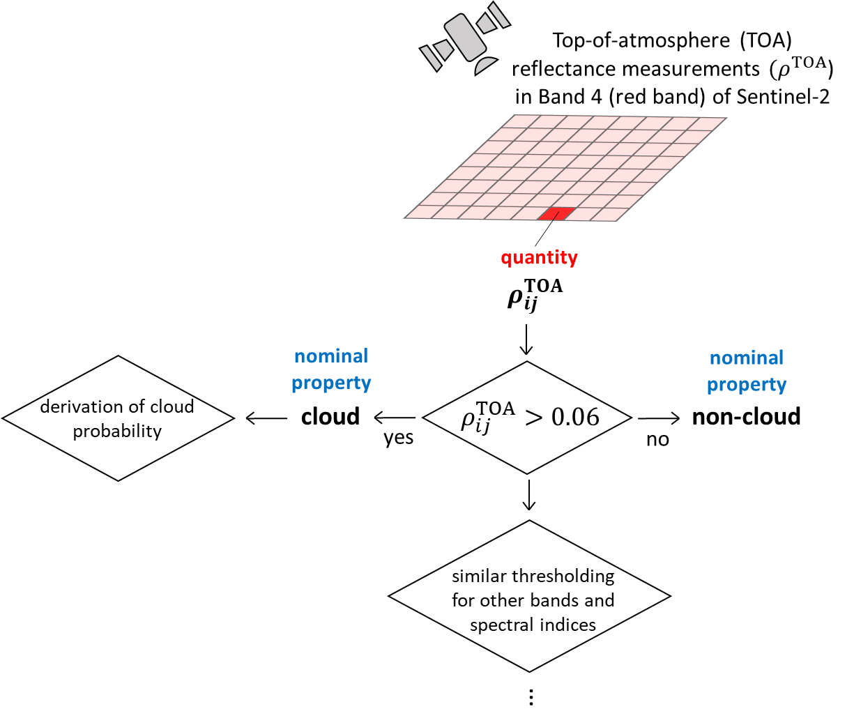
Figure 2: Cloud masking of Sentinel-2 satellite imagery.

Similarly to a probabilistic ML classifier, in conformity assessment the assigned category is provided with a probability value, the conformance probability. However, in conformity assessment the classifier is rule-based, there is no training phase, and therefore uncertainty related to a training phase does not need to be taken into account. For these reasons, the framework in [21] cannot be used for a comprehensive uncertainty evaluation of ML classifiers, which rely on training.

In a standard conformity assessment a threshold is fixed (e.g., a certain critical mass concentration of mercury based on which a water sample is considered to be conforming or non-conforming). In contrast, in a binary classification performed alike conformity assessment (e.g, cloud masking described above), a threshold is often empirically derived (e.g., based on expert knowledge of top-of-atmosphere reflectance of a cloud vs. non-cloud). In the latter case, there would be an additional uncertainty source associated with the choice of the threshold, which will affect the classification results, and this uncertainty source is not considered in a standard conformity assessment [21].

1.3 Summary of contributions

• We propose a metrological conceptual uncertainty evaluation framework for ML classification inspired by existing vocabularies and frameworks from the fields of qualitative chemical analysis [24] and clinical laboratory sciences [25]. It is based upon the determination of the PMF of the nominal variable returned by the ML classifier, and the expression of uncertainty in terms of summary statistics derived from it. We review some possible summary statistics, discussing their benefits and drawbacks. The framework represents a natural analogue to the determination of the PDF for a quantitative variable and the derivation from it of summary statistics such as standard uncertainty. We also show how conditional probability can be used to enable uncertainty evaluation for measurement models that have categorical variables as inputs.

• We illustrate our conceptual framework by applying it in the context of two case studies where a metrological approach adds value. The first is the use of ML for classification of land cover based upon surface reflectance measurements made by a spaceborne optical sensor. The second is the use of ML for detection of atrial fibrillation based upon photoplethysmography (PPG) signals used in wearable devices.

We present our conceptual framework in Sections 2 and 3. In Section 2, we show how the ML classification task can be viewed as the realisation of a nominal variable (nominal property), and we describe how such properties are addressed in metrology. In Section 3, we present our framework for uncertainty evaluation of nominal properties based on discrete probability distributions and summary statistics. We also address the propagation of uncertainty in ongoing traceability chains. We present our two case studies illustrating the framework in Section 4, before concluding in Section 5.

2 Examination of nominal properties

2.1 Nominal variables

Classification tasks deal with nominal variables. To explain what nominal variables are, we will use Stevens’ theory of scales of measurement [26], which is frequently cited to describe the nature of different types of variables involved in measurement. We note at the outset that the question as to whether the term measurement is applicable to all types of variables is a subject of extensive debate in the metrology community and return to this question later in the section. For a deeper review of Stevens’ theory and its relevance to metrology refer to [27]; see also other references which propose alternative scales of measurement to Stevens’ theory, e.g., [28], not considered in our study.

Stevens’ theory distinguishes four scales of measurement: nominal, ordinal, interval and ratio (see Table 1). A nominal scale has multiple categories (or classes) with no natural ordering, for example a biological species or a blood group. Although these categories can be represented by numbers, the numbers do not have any quantitative meaning. Variables measured on a nominal scale can only be compared based on their equality, i.e., same or different.

An ordinal scale also has multiple categories, but with a natural ordering. For example, wind force on the Beaufort scale or stages of cancer. Variables measured on an ordinal scale can be compared based on their equality and their order, e.g., higher/lower, stronger/weaker. Distances between categories, however, are not necessarily meaningful. For example, the difference in the severity of cancer stages I and II is not the same as the difference in the severity of cancer stages III and IV [29].

Unlike for an ordinal scale, for an interval scale the differences are meaningful. Examples of variables measured on an interval scale include longitude and latitude, year, etc. A distinctive feature of this scale is that it does not have a meaningful (‘true’) zero, which is chosen arbitrarily.

Variables measured on a ratio scale do have a ‘true’ zero and represent the most encountered variables in physics, for example length, mass, and electrical power.

Table 1: Stevens’ scales of measurement

Scale	Examples	Central tendency statistic	Dispersion statistic
nominal	biological species, blood group	mode	see Section 3
ordinal	wind force on the Beaufort scale, stage of cancer	median, mode	interquartile range (IQR)
interval	longitude and latitude, year	mean, median, mode	standard deviation, IQR
ratio	length, mass	mean, median, mode	standard deviation, IQR

One of the important aspects of the scales of measurement proposed by Stevens is that different scales have different statistics representing central tendency and dispersion. From a statistical point of view, a nominal scale represents the lowest (the most primitive) scale, while a ratio scale represents the highest scale. Statistical measures that apply to the lower scales also apply to the higher scales, but not the other way around [30]. For example, the central tendency of variables measured on a nominal scale can only be expressed by the mode, whereas the central tendency of variables measured on an ordinal scale can be expressed by the mode and the median. The notions of central tendency and dispersion are important for understanding how to express uncertainties. In Section 3, we discuss expressions of uncertainty for nominal variables.

The nomenclature for nominal variables varies across scientific communities. In the mathematical sciences, nominal and ordinal variables are often merged into a single group, categorical variables [30, 17], with nominal variables sometimes referred to as unordered categorical variables and ordinal variables referred to as ordered categorical variables [17]. In addition, nominal variables are sometimes called qualitative variables, and are distinguished from quantitative variables (variables measured on interval and ratio scales), with some ambiguity around the classification of ordinal variables [30]. However, in some international standards, the term qualitative variable (or qualitative property) is used as an umbrella term for both nominal and ordinal variables [29].

In this paper, we use the term categorical variable as an umbrella term for nominal and ordinal variables. We do not use the term qualitative variable to avoid confusion because, as mentioned above, there is disagreement about whether ordinal variables are included [30, 29]. We also use interchangeably the term variable (more common in the language of data science) and the term property (more common in the language of metrology).

Below, we will discuss how the evaluation of categorical (more specifically, nominal) variables is currently addressed in

• Authoritative metrological documents, namely the VIM and the GUM suite of documents;

• International standards;

• Metrology-related publications.

2.2 How nominal variables are addressed in…

2.2.1 Authoritative metrological documents

The authoritative metrological documents used to focus solely on quantities. This focus changed about a decade ago, when definitions of nominal properties and ordinal quantities were introduced in the 3${}^{\text{rd}}$ edition of the VIM, the VIM3 [1]. In the VIM3, a nominal variable is referred to as a nominal property and is defined as a [1, Definition 1.30]:

“property of a phenomenon, body, or substance, where the property has no magnitude

EXAMPLE 1 Sex of a human being.

EXAMPLE 2 Colour of a paint sample.

EXAMPLE 3 Colour of a spot test in chemistry.

EXAMPLE 4 ISO two-letter country code.

EXAMPLE 5 Sequence of amino acids in a polypeptide.

NOTE 1 A nominal property has a value, which can be expressed in words, by alphanumerical codes, or by other means.

NOTE 2 ‘Nominal property value’ is not to be confused with nominal quantity value.”

Interestingly, in the VIM3, ordinal variable is considered to represent a type of quantity. Correspondingly, it is referred to as an ordinal quantity and is defined as a [1, Definition 1.26]

“quantity, defined by a conventional measurement procedure, for which a total ordering relation can be established, according to magnitude, with other quantities of the same kind, but for which no algebraic operations among those quantities exist

EXAMPLE 1 Rockwell C hardness.

EXAMPLE 2 Octane number for petroleum fuel.

EXAMPLE 3 Earthquake strength on the Richter scale.

EXAMPLE 4 Subjective level of abdominal pain on a scale from zero to five.

NOTE 1 Ordinal quantities can enter into empirical relations only and have neither measurement units nor quantity dimensions. Differences and ratios of ordinal quantities have no physical meaning.

NOTE 2 Ordinal quantities are arranged according to ordinal quantity-value scales (see 1.28).”

In addition to providing definitions for nominal properties and ordinal quantities, the VIM3 clarifies that the term measurement relates only to quantities. In the VIM3, measurement is defined as [1, Definition 2.1] “the process of experimentally obtaining one or more quantity values that can reasonably be attributed to a quantity” with NOTE 1 explicitly stating that “measurement does not apply to nominal properties”. The VIM3 does not provide a separate entry for a term representing a measurement-like analogue for nominal properties. However, in Note 1 supplementing the definition of reference material [1, Definition 5.13], it says “Examination of a nominal property provides a nominal property value and associated uncertainty. This uncertainty is not a measurement uncertainty”, which implies that such an analogue is examination.

In the preparation of the 4${}^{\text{th}}$ edition of the VIM (the VIM4), the Joint Committee for Guides in Metrology (JCGM) is holding a discussion on including an entire chapter on nominal properties, motivated by the growing interest in a metrologically rigorous handling of these properties. These properties are indeed quite common in chemistry, forensics and clinical laboratory testing. An initial draft of the chapter is largely based on the vocabulary developed for clinical laboratory science by the IFCC (International Federation of Clinical Chemistry and Laboratory Medicine) and IUPAC (International Union of Pure and Applied Chemistry) [25].

Similarly to the VIM3, the vocabulary developed by the IFCC-IUPAC [25] differentiates measurement from examination. Unlike the VIM3, it provides an explicit definition of examination as “the process of experimentally obtaining one or more values that can reasonably be attributed to a nominal property together with any other available relevant information”, which is drafted analogously to the VIM3 definition of measurement. The IFCC-IUPAC vocabulary also introduces a term examinand (“nominal property intended to be examined”) analogous to the VIM3 definition of measurand (“quantity intended to be measured”). It is worth noting that in some other metrology-related publications, an additional term –– evaluation –– has been used as an umbrella term, which covers both measurement and examination [31], and the term evaluand used correspondingly to represent a property to be evaluated [32].

Whether the JCGM will adopt the terminology on nominal properties from the IFCC-IUPAC vocabulary [25] in the published version of the VIM4 is yet to be seen. However, the metrology community seems to be divided regarding whether two separate terms –– measurement and examination –– are necessary, or whether evaluation of nominal properties should be viewed as a type of measurement. In this latter direction, some publications by the national metrology institute of the United States of America, NIST (National Institute of Standards and Technology), use the term measurement and the term measurand for both quantitative and qualitative properties [33]. Similarly, in [27] –– a publication by the Measurement Standards Laboratory of New Zealand — a similar position is adopted, that the definition of measurement should be more inclusive and should cover evaluation of nominal variables in addition to quantities.

To summarise, the VIM3 provides explicit definitions of nominal properties and ordinal quantities. It also mentions that the term measurement does not apply to nominal properties, and the term examination should be used instead. However, it does not provide a separate entry for the definition of examination. The next edition of the VIM (VIM4) might bring more clarity as there is an ongoing discussion on including an entire chapter on the terminology related to nominal properties.

Unlike the VIM, the GUM suite of documents is entirely focused on quantities, with the only exception being the fourth document of the GUM suite dedicated to conformity assessment [21]. As previously stated in Section 1, in conformity assessment a measured quantity is converted into a nominal variable (either conforming and non-conforming). The relationship of conformity assessment to evaluation of nominal properties was previously discussed in guidelines produced by EURACHEM (European network of organizations focusing on analytical chemistry and quality related issues) and CITAC (The Cooperation on International Traceability in Analytical Chemistry) [24].

2.2.2 International standards

Although the VIM and the GUM currently provide negligible coverage of nominal variables, these variables have been addressed in a number of standards and recommendations produced by international bodies working in various areas of science and industry, where nominal variables are frequently used. As described above, a vocabulary dedicated to nominal variables – ”Vocabulary on nominal property, examination, and related concepts for clinical laboratory sciences (IFCC-IUPAC Recommendations 2017)” [25] – was developed by the International Federation of Clinical Chemistry and Laboratory Medicine (IFCC) and International Union of Pure and Applied Chemistry (IUPAC). Also, nominal variables and approaches to the evaluation of uncertainties associated with such variables were discussed in ”Assessment of performance and uncertainty in qualitative chemical analysis (EURACHEM/CITAC Guide)” [24]. Recommendations on handling nominal variables specifically related to reference materials, which have nominal properties, were recently systemised in the International Standard ISO 33406:2024 ”Approaches for the production of reference materials with qualitative properties” [29]. This ISO standard provides a discussion on establishing metrological traceability for reference material with nominal properties and evaluation of their uncertainties.

In relation to traceability of reference materials with nominal properties, ISO 33406:2024 advises that well-established guidelines on metrological traceability provided for quantities (e.g., ISO/IEC 17025 ”Testing and calibration laboratories” [34]) are followed whenever it is possible. Specifically, the metrological traceability guidelines should be used when the assignment of a nominal property relies on a measurement of a quantity (e.g., melting point or pH) and/or is performed in conditions that can be quantitatively assessed (e.g., times or temperatures) If, however, the assignment of a nominal property relies on the comparison with reference data or another reference material, which is already value-assigned for the nominal property in question, then this reference should be stated in the relevant documentation accompanying the reference material.

2.2.3 Metrology-related publications

The metrology community, including national metrology institutes and members of the JCGM working groups, has also been bringing more attention to nominal variables in its publications over the past years. Examples of the use of nominal variables in metrology and discussion on their uncertainty evaluation can be found in NIST reports (e.g. [35]). Evaluation of uncertainty for nominal variables was also previously discussed by members of JCGM Working Group 2 in [31]. It is important to note that although many of the above references address evaluation and expression of uncertainties associated with nominal variables, no agreement has yet been reached on this topic. And, to our knowledge, the discussion on the definition of uncertainty associated with nominal variables to be included in the VIM4 is still ongoing.

2.2.4 Summary

In recent years, interest in nominal properties has been growing in the metrology community, as reflected in several publications, standards and most importantly in the current work on the next edition of the VIM. However, no agreement has yet been reached on whether the term ‘measurement’ should cover nominal properties and on the expression of uncertainties associated with nominal variables. Section 3 will specifically address the latter.

3 Uncertainty evaluation for nominal properties

In this section, we outline approaches for uncertainty evaluation for nominal properties within ML classification models and further propagation through measurement models. In Section 3.1, we define PDFs and PMFs, illustrating that PMFs are the natural probability distribution for nominal properties. In Section 3.2, we describe various statistics that could be used to express uncertainty of nominal variables, highlighting their strengths and weaknesses. In Section 3.3, we show, with use of the PMF, how uncertainties of nominal properties can be propagated through measurement models having categorical inputs.

3.1 Probability distributions

As stated in the GUM [2] and other metrology-related publications [35], the uncertainty associated with any variable is fully expressed by its probability distribution, which is the distribution around a measured value (often taken as the mean of the distribution) in which the ‘true’ value is expected to lie. This distribution can either be empirical (i.e., based upon the frequency of occurrence of the variable), or have an assumed form (such as Gaussian). For continuous quantitative variables $\mathbf{x}$ that can take values in the set $\mathcal{X}\subset\mathbb{R}^{D}$, where $D$ is the dimension of the continuous input space, the probability distribution is defined in terms of a probability distribution function (PDF), which is a map or function

$$p:\mathcal{X} \rightarrow \mathbb{R}^{+},$$

$$\mathbf{x} \mapsto p(\mathbf{x}),$$ (3.1)

where

$$\int_{\mathcal{X}}p(\mathbf{x})\,\mathrm{d}\mathbf{x}=1.$$ (3.2)

Condition (3.2) ensures that $p(\mathbf{x})$ is properly normalised and can act as a PDF.

Similarly, for a nominal variable with $K$ possible classes (or categories), that can take values in the set $\mathcal{C}_{K}=\{c_{1},\dots,c_{K}\}$, the probability distribution is defined in terms of the PMF:

$$p:\mathcal{C}_{K} \rightarrow [0,1],$$

$$c_{k} \mapsto p_{k}:=p(c_{k}),$$ (3.3)

where

$$\sum_{k=1}^{K}p_{k}=1.$$ (3.4)

Condition (3.4) ensures $p$ obeys the correct probability sum rule and can act as a PMF.

The PMF of a nominal property can also be fully described in terms of its probability vector

$$\mathbf{p}=[p_{1},\dots,p_{K}]\in[0,1]^{K},$$ (3.5)

where each element of the array can take values on the interval $[0,1]$, and condition (3.4) also holds.

Given the analogy with PDF for quantitative variables, the PMF is the natural candidate for expressing uncertainty in nominal properties and has been motivated in metrology-related publications such as [31, 33], as well as the recent international standard [29] introduced in Section 2.2.2.

3.2 Expressions of uncertainty

Expressions of uncertainty for quantitative variables such as the standard deviation are well known in the metrology community, and are used in the GUM [36]. The standard deviation is one example of a summary statistic which expresses the uncertainty of a quantitative variable in terms of a single positive real number. More formally, given a quantitative variable $\mathbf{X}$ with PDF $p(\mathbf{x})$, a statistic $u$ for uncertainty is evaluated using a function $F$ such that

$$u=F(p(\mathbf{x})),\quad u\in[0,\infty).$$ (3.6)

Statistics calculated from a function $F$, such as the standard deviation or interquartile range (IQR), are measures of dispersion about a central tendency (see Table 1). Defining a statistic of dispersion for nominal properties is more challenging as the only statistic of central tendency is the mode, for which there is no natural notion of distance [31]. Thus, the more common way to express uncertainty of nominal properties is in terms of statistics (or indices) of variation [37, 31]. However, there is debate in the metrology community about the nomenclature for describing various uncertainty statistics of nominal properties in terms of variation or dispersion, such as the information entropy [25, 31] (see Section 3.2.2 for a definition). In this section we will avoid use of such terminology, and focus on the mathematical properties and their implications as candidates for expressions of uncertainty in nominal properties.

The first point to note is the distinction made in the literature e.g., [31, 38], between the confidence in the prediction of an ML classification model, and the predictive uncertainty. Given a probability vector $\mathbf{p}=[p_{1},,\dots,p_{K}]$ of an ML classification model $y=f(x),\,y\in\mathcal{C}_{K}$, the classification of the output is typically given by the mode of the PMF:

$$\mathrm{mode}=\underset{k}{\arg\max}(\mathbf{p)}.$$ (3.7)

The confidence in the prediction can then be expressed as $p_{\mathrm{mode}}$, which is the probability that $y$ is the modal class $c_{\mathrm{mode}}$, also known as the modal probability. Note that this is distinct from a confidence interval which is used to express uncertainty for quantitative variables in the GUM and the VIM.

Using the modal probability as a form of expression has advantages in the sense that it is directly associated with the model prediction, and as such aligns with the language for expressing uncertainty of quantitative variables [2]. For example, the output of a classification model $\widehat{y}=f(x)$ can be written as the pair $(c_{\mathrm{mode}},p_{\mathrm{mode}})$, where $p_{\mathrm{mode}}$ is the confidence in the prediction that $\widehat{y}=c_{\mathrm{mode}}$. This language can be extended [31] to include multiple classes, i.e., the ML classification model predicts $\widehat{y}=\{c_{1},c_{2}\}$ with probability $p=p_{1}+p_{2}$. However, confidence is not the same as uncertainty. A confidence equal to $1$ would express complete certainty in the output of a classification model, thus the uncertainty should be $0$.

3.2.1 Properties of an uncertainty statistic

In general, a statistic $F$ expressing the uncertainty associated with a nominal variable $y$ with PMF $\mathbf{p}$, should satisfy the following properties (adapted from [37, 39]):

1. $F$ gives a positive real scalar value: $F(\mathbf{p})\in[0,\infty)$.

2. $F$ gives $0$ when there is no uncertainty. That is, $F(\mathbf{p}^{1})=0$, where

   $$p^{1}_{k}=\begin{cases}1,&k=\mathrm{mode},\\ 0,&\text{otherwise.}\end{cases}$$

3. $F$ is maximum when there is maximal uncertainty. This is when all probabilities are equal:

   $$F(\mathbf{p})\leq F(\mathbf{p}_{\text{unif}}),$$

   where $(p_{\text{unif}})_{k}=1/K,\,k=1,\dots,K$ is the categorical uniform distribution.

A normalised statistic $F_{\mathrm{norm}}$ can then be defined for nominal properties:

$$F_{\mathrm{norm}}(\mathbf{p})=\dfrac{F(\mathbf{p})}{F(\mathbf{p}_{\text{unif}})}\in[0,1],$$ (3.8)

where $F_{\mathrm{norm}}(\mathbf{p}_{\text{unif}})=1$ represents maximal uncertainty.

In summary, a (normalised) statistic $F$ expressing the uncertainty associated with the output probabilities of an ML classification model is minimum (zero) when the model predicts equal probabilities to all classes, and is maximum (one) when the model predicts a single class with $100\,\%$ probability.

In the following analysis, we will consider only normalised statistics that satisfy the above properties, for a fair comparison between expressions of uncertainty. As such, we do not consider statistics that quantify different aspects of uncertainty, such as the expected difference of information [40], which has been gaining popularity in land cover classification (see case study in Section 4.1). This statistic requires identification of a reference class, which fails on property 3, since the reference probability is minimum for a uniform distribution.

3.2.2 Information entropy

The information (or Shannon) entropy (not to be confused with thermodynamic entropy) is an expression of information content, originally motivated to describe the theory of signal communication [41].

The normalised version (or relative probability entropy) is defined for nominal properties as

$$H(\mathbf{p})=\mathbb{E}[-\log_{K}\mathbf{p}]=-\sum_{k=1}^{K}p_{k}\log_{K}p_{k}.$$ (3.9)

Information entropy is commonly used in the existing literature as a statistic for expressing the uncertainty in nominal variables [32, 37, 42], as well as the recent international standard [29]. It is also the most commonly used statistic in the ML community for summarising uncertainty in predictions of classification models [16, 38, 12]. The principle of maximum entropy (uncertainty) is also used in Bayesian inference (see Section 4.1.3) for selection of prior probabilities [43].

Mari [31] suggested an extension to information entropy given (in normalised form) by

$$H^{*}(\mathbf{p})=\dfrac{K^{H(\mathbf{p})}-1}{K-1}=\dfrac{\prod_{k=1}^{K}p_{k}^{-p_{k}}-1}{K-1}.$$ (3.10)

Such a transformation can be performed to any expression of uncertainty $F(\mathbf{p})$ for nominal properties to produce a new statistic $F^{*}(\mathbf{p})=(K^{F(\mathbf{p})}-1)/(K-1)$, which also satisfies the properties in Section 3.2.1. This transformation has the property $F^{*}(\mathbf{p})\leq F(\mathbf{p})\,\forall\,\mathbf{p}$, and so will lower the variation in the values of the new statistic (see Figures 5 and 7). This allows the statistic to be more robust against small perturbations of the PMF.

One alternative variant on the information entropy is called the $\alpha$-quadratic entropy [44], defined as

$$H_{\alpha}(\mathbf{p})=\frac{K^{2\alpha-1}}{(K-1)^{\alpha}}\sum_{k=1}^{K}p_{k}^{\alpha}(1-p_{k})^{\alpha},\quad\alpha\in(0,1].$$ (3.11)

If $\alpha$ is close to zero, this statistic is not very sensitive to changes in $\mathbf{p}$, but for $\alpha$ close to one, this statistic has higher sensitivity [45], and has been used in evaluating uncertainties in land cover classification models [45, 46]. We consider the case when $\alpha=1$ in Section 3.2.6.

3.2.3 Wilcox’s variation ratio

Wilcox’s variation ratio (WVR) [37], also known as the mean deviation from the mode, is a natural extension of the concept of confidence in a classification model prediction to an expression of uncertainty, defined by

$$u_{\mathrm{WVR}}(\mathbf{p})=1-\dfrac{Kp_{\mathrm{mode}}-1}{K-1}.$$ (3.12)

The WVR expresses the remaining uncertainty after taking into account the modal probability $p_{\mathrm{mode}}$ of the classification result. However, it does not take into account the entire PMF, so is ignorant of variation in probabilities of the remaining classes. This issue is only relevant in the case of non-binary classification problems, such as that described in Section 4.1.

3.2.4 Universal variation ratio

The WVR is undefined in the case of multimodal distributions, where more than one class is equally likely. The universal variation ratio (UVR) [47] is an extension of the WVR that takes account of multimodal distributions, defined as

$$u_{\mathrm{UVR}}(\mathbf{p})=\dfrac{K^{2}}{K^{2}-1}\left(1-\dfrac{p_{\mathrm{mode}}}{c}\right),$$ (3.13)

where $c$ is the number of modes. It can be shown [47] that $u_{\mathrm{UVR}}(\mathbf{p})\leq u_{\mathrm{WVR}}(\mathbf{p})$ for all unimodal distributions.

3.2.5 Standard deviation from the mode

Both the WVR and UVR take account of the modal probability $p_{\mathrm{mode}}$ only, but not the distribution among the remaining classes, which might be important to consider. Although information entropy takes account of all class probabilities, there is no notion of “distance” from the central tendency. Motivated by finding an equivalent to the standard deviation about the mean for quantitative variables, a standard deviation from the mode (SDM) for nominal variables [48] can be defined as

$$u_{\mathrm{SDM}}(\mathbf{p})=1-\sqrt{\dfrac{\sum_{k=1}^{K}(p_{\mathrm{mode}}-p_{k})^{2}}{K-1}}.$$ (3.14)

The SDM has the property that $u_{\mathrm{SDM}}(\mathbf{p})\leq u_{\mathrm{WVR}}(\mathbf{p})$ for all unimodal distributions.

One advantage of using the SDM is that for a large number $n$ of samples used to estimate the output PMF, such as the output trees of random forests, the SDM is normally distributed [48] $\widehat{u}_{\mathrm{SDM}}\sim\mathcal{N}(u_{\mathrm{SDM}}(\mathbf{p}),\sigma_{\mathrm{SDM}}^{2}(\mathbf{p}))$ with

$$\sigma_{\mathrm{SDM}}^{2}(\mathbf{p})=\dfrac{p_{\mathrm{mode}}(1-Kp_{\mathrm{mode}})^{2}+\sum_{k=1}^{K}p_{k}(p_{\mathrm{mode}}-p_{k})^{2}}{n(K-1)^{2}(1-u_{\mathrm{SDM}}(\mathbf{p}))^{2}}-\dfrac{(1-u_{\mathrm{SDM}}(\mathbf{p}))^{2}}{n}.$$ (3.15)

This result allows the use of confidence intervals for the statistic.

3.2.6 Index of qualitative variation

The index of qualitative variation (IQV) [37], also known as the quadratic score [49], is another common expression of uncertainty that is widely accepted in the social sciences [47]. It is defined in normalised form as

$$u_{\mathrm{IQV}}(\mathbf{p})=\dfrac{K}{K-1}\left(1-\sum_{k=1}^{K}p_{k}^{2}\right).$$ (3.16)

The IQV is a special case of the $\alpha$-quadratic entropy in expression (3.11) with $\alpha=1$.

3.2.7 Coefficient of nominal variation

A variant of the IQV proposed in [50] is the coefficient of nominal variation (CNV) defined as

$$u_{\mathrm{CNV}}(\mathbf{p})=1-\sqrt{1-u_{\mathrm{IQV}}(\mathbf{p})}=1-\sqrt{\dfrac{K\sum_{k=1}^{K}p_{k}^{2}-1}{K-1}}.$$ (3.17)

This transformation ensures that $u_{\mathrm{CNV}}(\mathbf{p})\leq u_{\mathrm{IQV}}(\mathbf{p})$ for all distributions, with equality for $\mathbf{p}^{1}$ and $\mathbf{p}_{\text{unif}}$. In terms of the normed distance $d(\mathbf{p},\mathbf{q})=||\mathbf{p}-\mathbf{q}||_{2}$ between two PDFs $\mathbf{p}$ and $\mathbf{q}$, the CNV can be rewritten as

$$u_{\mathrm{CNV}}(\mathbf{p})=1-\dfrac{d(\mathbf{p},\mathbf{p}_{\text{unif}})}{d(\mathbf{p}^{1},\mathbf{p}_{\text{unif}})},$$

giving the CNV a natural interpretation in terms of the distance of the PMF from a uniform distribution.

3.2.8 Comparing statistics of uncertainty

The statistics described in Section 3.2 have various advantages and disadvantages. In this section we compare their properties and performance on a few example predictive probability distributions. One particular example in binary classification is the PMF $\mathbf{p}_{A}$ shown in Figure 3. Since $\mathbf{p}_{A}$ is halfway between total certainty and maximal uncertainty, it was suggested in [39] that the statistic of uncertainty should also be halfway between the extreme values, i.e., 0.5. We also consider the multi-class PMFs $\mathbf{p}_{B}$ and $\mathbf{p}_{C}$, which have the same model prediction $\widehat{y}$, with the same confidence (modal probability) of 0.5 (see Figure 3).

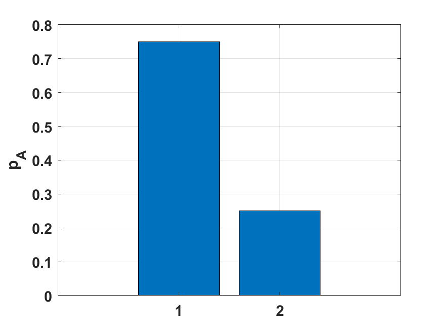
(a) Example binary classification PMF: $\mathbf{p}_{A}=[0.75,0.25]$.

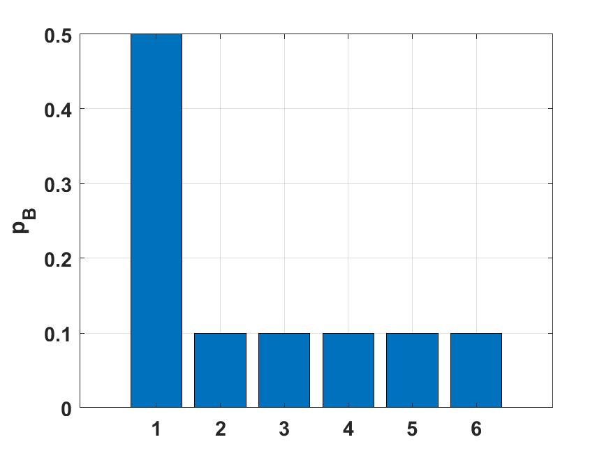
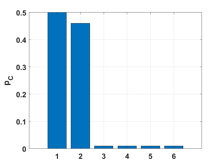
(b) Example multi-class classification PMFs: $\mathbf{p}_{B}=[0.5,0.1,0.1,0.1,0.1,0.1]$ and $\mathbf{p}_{C}=[0.5,0.46,0.01,0.01,0.01,0.01]$.

Figure 3: Example predictive PMFs as output from ML classifiers.

Table 2 compares the various expressions of uncertainty for nominal properties. The first point to note is the result that $F(\mathbf{p}_{B})\geq F(\mathbf{p}_{C})$ for all $F$ considered, even though it seems more obvious which is the best prediction of the classification model in $\mathbf{p}_{B}$. That is because the statistics are expressing the certainty that the mode can either be one of two possibilities (i.e. $(p_{C})_{1}+(p_{C})_{2}=0.96$ for $\mathbf{p}_{C}$), whereas there is more spread in the distribution of $\mathbf{p}_{B}$.

If we expect the uncertainty of $\mathbf{p}_{A}$ to be 0.5, then we see that WVR, SDM and CNV satisfy this condition. If information about the modal probability is to be used explicitly and information about the entire distribution is to be used, then SDM is the only option. However, the SDM shows little difference in uncertainty between $\mathbf{p}_{B}$ and $\mathbf{p}_{C}$, where a larger difference from studying Figure 3 might be expected to be seen. In this case, CNV might be the more appropriate choice, but at the cost of not explicitly using the modal probability.

We specify in Table 2 whether a particular statistic is well-defined (Y) or not well-defined (N) in the pathological multimodal case where two or more classes share precisely the same modal probability. However, the definition of these statistics can be trivially extended to the multimodal case by arbitrarily choosing the mode to be any of the maximum probability classes, this choice not affecting the value of the statistic.

Table 2: A comparison of expressions of uncertainty for nominal properties.

Statistic	Uses $p_{\mathrm{mode}}$	Uses full PMF	Multimodal	$\mathbf{p}_{A}$	$\mathbf{p}_{B}$	$\mathbf{p}_{C}$
$H$ (3.9)	N	Y	Y	0.81	0.84	0.50
$H^{*}$ (3.10)	N	Y	Y	0.75	0.69	0.29
WVR (3.12)	Y	N	N	0.50	0.60	0.60
UVR (3.13)	Y	N	Y	0.33	0.51	0.51
SDM (3.14)	Y	Y	N	0.50	0.60	0.56
IQV (3.16)	N	Y	Y	0.75	0.84	0.65
CNV (3.17)	N	Y	Y	0.50	0.60	0.40

3.3 Uncertainty propagation with nominal properties

In Section 3.2, we considered various ways in which the uncertainty in nominal properties can be expressed through a summary statistic. However, to propagate such uncertainty through a chain of measurement models, it is more appropriate to consider the full PMF. For quantitative properties, it is more difficult to propagate the full PDF analytically due to intractable integrals, and it is commonly the case that the full PDF is unknown and modelled using simpler forms such as assuming a Gaussian distribution. In such cases, summary statistics, such as the standard deviation, are propagated using the law of propagation of uncertainty [2]. Alternatively, where the PDF is well known, sampling techniques such as Monte Carlo (MC) can propagate the full PDF [18].

In the case of a PDF having an analytical form, such as a Gaussian or rectangular distribution, the full PDF can be directly inferred from summary statistics, such as the standard deviation. On the other hand, the summary statistics for nominal properties described in Section 3.2 cannot be used to infer the PMF except in a few very niche examples. This property also supports the use of the full PMF in uncertainty propagation in traceability chains that involve nominal properties.

Since, for nominal properties, the PMF can be defined explicitly, it can be used to obtain analytical results for propagation through measurement models. Consider an ML classification model $f$ with outputs $y\in\mathcal{C}_{K}$, which have a predictive distribution $\mathbf{p}=[p_{1},\dots,p_{K}]$. Assume the outputs $y$ become inputs to the next measurement model $g$, which has both nominal and quantitative input variables, in the form of a $D$-dimensional vector $\mathbf{x}$, and outputs a quantitative variable $z\in\mathbb{R}$:

$$z=g(\mathbf{x},y),\quad\mathbf{x}\in\mathcal{X}\subset\mathbb{R}^{D},\,y\in\mathcal{C}_{K},\,z\in\mathbb{R}.$$ (3.18)

Since there are $K$ possible values for $y$, we can describe $g$ as a model conditioned on a nominal variable, and therefore express $g$ in terms of $K$ models $z=g(\mathbf{x},c_{k})=g_{k}(\mathbf{x})$, where $\mathbf{x}\in\mathcal{X}_{k}\subset\mathbb{R}^{D}$ for $k=1,\dots,K$. This expression can be thought of as modelling a system which has $K$ different regimes, defined by the classes $c_{k}$.

The expected value of the output $z$ can be expressed in terms of the expected values of the functions $g_{k}(\mathbf{x})$:

$$\mathbb{E}[z]=\sum_{k=1}^{K}p_{k}\int_{\mathcal{X}_{k}}d\mathbf{x}\,q_{k}(\mathbf{x})g(\mathbf{x},c_{k})=\sum_{k=1}^{K}p_{k}\int_{\mathcal{X}_{k}}d\mathbf{x}\,q_{k}(\mathbf{x})g_{k}(\mathbf{x})=\sum_{k=1}^{K}p_{k}\mu_{k},$$ (3.19)

where $q_{k}(\mathbf{x})$ are the PDFs of the input variable $\mathbf{x}\in\mathcal{X}_{k}$ and $\mu_{k}=\mathbb{E}_{\mathbf{x}\sim q_{k}(\mathbf{x})}[g_{k}(\mathbf{x})]$. The means $\mu_{k}$ can be evaluated in the standard way for quantitative input variables.

We can also compute the variance of the output $z$:

$$\text{Var}[z] =\mathbb{E}[z^{2}]-\mathbb{E}[z]^{2}$$

$$=\sum_{k=1}^{K}p_{k}\mathbb{E}[g_{k}(\mathbf{x})^{2}]-\sum_{j,k=1}^{K}p_{j}p_{k}\mu_{j}\mu_{k}$$

$$=\sum_{k=1}^{K}p_{k}(\text{Var}[g_{k}(\mathbf{x})]+\mu_{k}^{2})-\sum_{j,k=1}^{K}p_{j}p_{k}\mu_{j}\mu_{k}$$

$$=\sum_{k=1}^{K}p_{k}\sigma_{k}^{2}+\sum_{j,k=1}^{K}p_{j}p_{k}(\mu_{k}^{2}-\mu_{j}\mu_{k}),$$

where $\sigma_{k}^{2}=\text{Var}_{\mathbf{x}\sim q_{k}(\mathbf{x})}[g_{k}(\mathbf{x})]$ can be evaluated using the methods described in [2] for computing expressions of uncertainty in quantitative variables.

For this simple example, the moments of the measurand given nominal property inputs can be determined analytically. More generally, MC techniques can be applied by sampling directly from the PMF to determine the output PDF $p(z)$. Proceeding in this way is relevant to measurement applications that depend upon a prior classification, such as in determining particle concentration from counting measurements [51].

4 Case studies

In this section we present two applications of uncertainty evaluation using ML classification models: Land cover classification (Section 4.1), and atrial fibrillation detection using PPG signal data (Section 4.2). In both cases we describe the background on the challenge, methods for obtaining class probabilities, and exploration of the contributions of different sources of uncertainty.

4.1 Land cover classification

4.1.1 Background

Land cover (LC) maps produced by classification of satellite imagery provide essential information on the Earth’s biophysical cover. This information serves as an important input into a variety of applications, e.g.

• Hydrological and climate modelling [52, 53], where LC maps are used for setting up land surface conditions;

• National greenhouse gas accounting [54], where LC maps along with additional data are used for estimation of emissions associated with anthropogenic land use;

• Biodiversity monitoring [55], where LC maps provide information on habitats and their fragmentation, etc.

Evaluation of uncertainties associated with LC maps is important both in its own right for the interpretation of such maps, and for the propagation of these uncertainties further – to the downstream applications of LC maps mentioned above. As stated in Section 3.3, propagation of uncertainties of a nominal variable requires its full PMF. This PMF should include contributions of all uncertainty sources mentioned in Section 1.2 and illustrated in Figure 1.

LC mapping is a multi-class classification problem, which currently is widely approached by ML. The most popular ML classification models used for LC mapping are tree-based models (such as random forests) [56, 57, 58, 59], and convolutional neural networks (CNNs) [60, 61]. There are many LC classification schemes. Some classification schemes include only a few, very broad, classes, e.g., tree cover, grassland, cropland, etc. [62], whereas other classification schemes provide finer details, e.g. they distinguish broad-leaved and coniferous forest [63]. Some classification schemes have a nested structure where broad classes are further split into narrower classes [58]. It is important to note that in the present case study we approach land cover classification in similar fashion to how it is commonly approached in the literature – as a classification problem with a univariate output, i.e., each pixel considered separately. An important extension would be to perform classification with a multivariate output. In this case, classification would produce a collection of output variables (a collection of LC classes) corresponding to multiple pixels as opposed to each single pixel. Such an extension would make sense given how strongly correlated EO data typically is in the spatial domain.

4.1.2 Data

As previously mentioned in Section 1.1, a supervised ML classification model is trained on a data set consisting of pairs of several input variables and a categorical output. In our LC classification study, the input variables represented surface reflectance measurements performed in ten spectral bands of Sentinel-2 satellite over a single pixel. The output variable represented LC class in that pixel. Information on LC classes (i.e., LC labels) is typically obtained either manually (by visual interpretation of high/very high resolution satellite imagery or by ground surveys), automatically (e.g., based on pre-existing LC maps), or hybrid-like (following a combination of the two methods) [64]. In our study, LC labels were obtained by an automatic collection procedure following a modified approach of UK Centre for Ecology and Hydrology (UKCEH), used for the collection of training data for the production of UK annual LC maps [57]. This method relies on the assumption that LC change is gradual. It uses UKCEH LC maps produced for three previous years to find pixels with stable LC classes (i.e. unchanged LC classes throughout these years). Further filtering was performed to identify such unchanged pixels where the RF classifier used by the UKCEH to produce their LC maps yielded a probability greater than 95 %. In other words, we only retained pixels, where the LC label was assigned with the highest confidence. For the present case study, LC labels were collected over a $20\,\text{km}\times 20\,\text{km}$ area of interest (AOI) in Scotland. The collection process yielded 189,142 unchanged pixels (i.e., 4.7 % of the AOI) corresponding to forest, cropland, grassland and settlements classes.

The input variables (i.e., surface reflectance measurements) for the 189,142 unchanged pixels were retrieved from Sentinel-2 images collected over the AOI on the 1st of June, 2020 and 2021. Although space-borne surface reflectance measurements have many uncertainty sources associated with them, in the present study we choose to focus on one uncertainty source. This uncertainty source is related to the imperfect knowledge of aerosol optical depth (AOD) used in the atmospheric correction of the satellite imagery. It represents just one (although ordinarily dominant) contribution to the uncertainty sources (1) and (5) described in Section 1.2 and illustrated in Figure 1. The AOD uncertainties were introduced into the atmospheric correction process by Monte Carlo (MC) sampling (we used 25 MC samples). This process yielded 25 realizations of surface reflectance measurements for each of the 189,142 unchanged pixels. See [14] for more details on the data set.

4.1.3 Propagation of uncertainties within Bayesian classification models

As illustrated in Figure 1, ML classification models come with multiple sources of uncertainty. Most of these sources can be described in terms of probability distributions for particular parametric classification models (such as Naïve Bayes, logistic regression, discriminant analysis [13] and neural networks [65]) that naturally lend themselves to a Bayesian treatment. In this section we describe a framework that can be followed to incorporate these sources of uncertainty for Bayesian generative ML classifiers, which explicitly model the input data uncertainties.

Let $\mathcal{D}=\{(\mathbf{x}_{i},y_{i})|i=1,\dots,N\}$ be the training data consisting of $N$ pairs of input and output observations, where $\mathbf{x}_{i}\in\mathcal{X}\subset\mathbb{R}^{p}$ and $y_{i}\in\mathcal{C}_{K}$. Then we can model the sources of uncertainty described in Figure 1 in the following way:

• The training data uncertainty (1) from a measurement process can be described in terms of a probability distribution $p(\mathbf{x})$.

• The class assignment uncertainty of the ML classification task (2) derives from the joint empirical probability distribution $p(\mathbf{x},y)$. This can be separated into two contributions via Bayes’ rule

  $$p(\mathbf{x},y=c_{k})=p(\mathbf{x}|y=c_{k})p(y=c_{k}),\quad k=1,\dots,K.$$ (4.1)

  $p(\mathbf{x}|y=c_{k})$ is the class conditional probability distribution describing the distribution of the input data for each class. $p(y=c_{k})$ is the probability distribution describing the prior class distribution (or class imbalance) in the training data.

• ML models also come with model hyperparameters, which describe the choice of model (3), such as model architecture or optimisation method. Various hyperparameter optimisation tuning methods [66] can be used to determine the optimal model choice. Bayesian optimisation is one popular approach [67], and for such an approach, quantification of the uncertainties in choice of model has been attempted [68].

• A parametric classification model can be described by a probability distribution $p(y_{i}|\mathbf{x}_{i},\theta)$, where $\theta$ are the parameters of the model. The uncertainty associated with such a model is given by the probability distribution of the model parameters. The likelihood function $\mathcal{L}$ of the model is expressed in terms of the model distribution on the training data, and any additional training data uncertainty

  $$\mathcal{L}(\mathcal{D}|\theta)=\prod_{i=1}^{N}p(\mathbf{x}_{i},y_{i}|\theta)=\prod_{i=1}^{N}p(y_{i}|\mathbf{x}_{i},\theta)p(\mathbf{x}_{i}).$$ (4.2)

  In a Bayesian setting, Bayes’ rule is used to determine the posterior distribution in the model parameters (4) (otherwise known as Bayesian inference)

  $$p(\theta|\mathcal{D})=\dfrac{\mathcal{L}(\mathcal{D}|\theta)p(\theta)}{p(\mathcal{D})}.$$ (4.3)

  The Bayesian approach introduces an additional uncertainty $p(\theta)$, which is the prior distribution on the model parameters. This can be determined from expert knowledge, or one can use conjugate priors [13] if known for analytic determination of the posterior. $p(\mathcal{D})$ is known as the evidence, and is typically intractable for more complex classification models such as CNNs. In such cases one must resort to sampling techniques such as Markov Chain Monte Carlo (MCMC) [69], approximation techniques such as variational inference [13] or MC dropout [16] to estimate the posterior distribution.

• Just as with training input data, new input data also comes with measurement uncertainty (5). This can be described in terms of a probability distribution $p(\mathbf{x}_{\mathrm{new}})$.

• The probability distribution associated with the new input data uncertainty on an input $\mathbf{x}_{\mathrm{new}}$ (known as the posterior predictive) can be evaluated as the expectation of the ML model probability of class $k$ with respect to the uncertainty in the model parameters $p(\theta|\mathcal{D})$:

  $$p(y_{\mathrm{pred}}=c_{k}|\mathbf{x}_{\mathrm{new}},\mathcal{D})=\mathbb{E}_{\theta|\mathcal{D}}\left[P(y_{\mathrm{pred}}=c_{k}|\mathbf{x}_{\mathrm{new}},\theta)\right]$$ (4.4)

The posterior predictive distribution of the ML classification model can then be written in the form of a PMF with probability vector $\mathbf{p}=[p_{1},\dots,p_{K}]^{\top}$, where $p_{k}:=p(y_{\mathrm{pred}}=c_{k}|\mathbf{x}_{\mathrm{new}},\mathcal{D})$. This PMF can then by used to propagate uncertainties in further measurement models where the output of the ML classification model is used as an input, either analytically (as shown in Section 3.3), or through MC sampling of the PMF.

4.1.4 Numerical examples

We apply the Bayesian framework described in Section 4.1.3 to the datasets described in Section 4.1.2, using the Bayesian quadratic discriminant analysis model presented in [14]. Specifically we compute the posterior predictive probabilities on test sets ($90\,\%$ of available pixels) from years 2020 and 2021, with training set taken from the remaining $10\,\%$ of pixels from year 2020.

The confusion matrices (comparing class predictions and “true” class labels) from taking the maximum probability as the predicted class are given in Figure 4. We include the true/false positive and true/false negative rates to see how the model performs on each class, as well as computing the overall classification loss, which is the misclassification rate, or fraction of class predictions not from the true labelled class.

For evaluation of the performance of the output class probabilities from the classification models, we use two expected values of proper scoring rules [70], namely the multi-class cross-entropy loss (XE) and the Brier score (BS). Proper scoring rules are a principled way to measure the quality of the predictive probabilities produced by ML classification models [71].

Assume we have an ML classification model and a test dataset with $N$ observations (i.e. pixels in the case of land cover). For each observation $i=1,\dots,N$, the test dataset has a class label $k=1,\dots,K$. This can be represented by the binary matrix $y_{ik}$, where $y_{ik}=1$ if test observation $i$ has class label $k$, and zero otherwise. The output predictive probabilities of the model for each test observation $i$ and class label $k$ is represented by the probability matrix $p_{ik}$. The XE and BS for each test observation $i$ are then defined as

$$\mathrm{XE}_{i}=-\sum_{k=1}^{K}y_{ik}\log(p_{ik}),\qquad\mathrm{BS}_{i}=\frac{1}{K}\sum_{k=1}^{K}(y_{ik}-p_{ik})^{2},$$ (4.5)

The XE is similar to the information entropy defined in Section 3.2.2 except that instead of only using the probability of being the most likely class from the model output, the output probabilities are used to calculate agreement to an independent test dataset, so that ‘predictive performance’ is evaluated. The XE is commonly used in neural networks classifiers as the objective function to minimise during training. The BS is the mean squared difference between the test class label and the predicted probability. It considers all output probabilities, whereas XE only considers the probability associated with the test class label.

To evaluate overall performance, we take expected values over the XE and BS defined in expression (4.5) for each test pixel $i$, as well as normalising the values such that 0 is perfect prediction, and 1 represents a predictive performance no better than using the prior class distribution of the test dataset as a trivial classifier (i.e. the fraction of land cover class abundance within the AOI). The expected XE (EXE) and BS (EBS) are defined as

$$\mathrm{EXE}=\frac{1}{N}\sum_{i=1}^{N}\frac{\sum_{k=1}^{K}y_{ik}\log(p_{ik})}{\sum_{k=1}^{K}q_{k}\log(q_{k})},\qquad\mathrm{EBS}=\frac{1}{N}\sum_{i=1}^{N}\frac{\sum_{k=1}^{K}(y_{ik}-p_{ik})^{2}}{\sum_{k=1}^{K}q_{k}(1-q_{k})},$$ (4.6)

where $q_{k}$ is PMF of classes $k$ from the test dataset prior to ML classification.

The resulting metric values for test year 2020 were: classification loss = 0.0122; EXE = 0.0789; EBS = 0.0312. For test year 2021: classification loss = 0.0572; EXE = 0.5673; EBS = 0.1514. As is common with ML classification tasks, we see a degradation in performance when the model is tested on data outside the training domain (in this case a different year). We also observe from Figure 4 that the class ‘settlements’ have the highest false positive rate. This is in large part due to the low abundance of settlement pixels within the AOI, and so the ML classifier will tend to give other land cover classes with larger abundances a higher predictive probability.

(a) Test Year: 2020

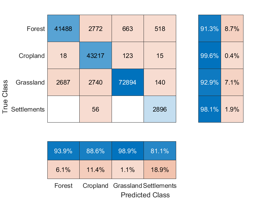
(b) Test Year: 2021

Figure 4: Confusion matrices using Bayesian QDA. Final column corresponds to the true/false positive rates for each class. Final row corresponds to true/false negative rates.

In addition to the classification results, we also compute the expressions of uncertainty for nominal properties described in Section 3.2 using the posterior PMFs obtained within the Bayesian framework of [14]. Figure 5 shows box and whisker plots [72] in the chosen uncertainty statistics, capturing the median, interquartile range (IQR), as well the limit of non-outliers (given by $1.5\times\text{IQR}$ away from the top or bottom box). Due to the high accuracy of the LC classifiers, all statistics had values very close to zero, so the median cannot be visualised. This also makes the distributions in the statistics highly skewed.

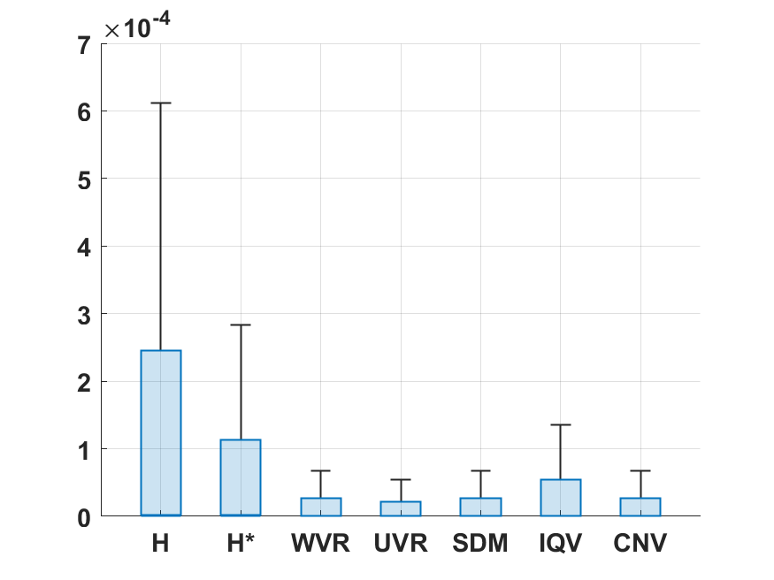
(a) Test Year: 2020

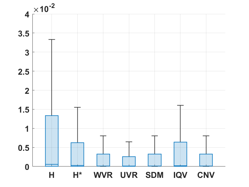
(b) Test Year: 2021

Figure 5: Box and whisker plots of uncertainty statistics for LC classification using Bayesian QDA.

Note the large difference in scales in Figure 5 from years 2020 to 2021. This is due to the large classification performance degradation observed in the classification metrics from years 2020 to 2021 (see Figure 4), causing the resulting predictive PMFs to be more uncertain. However, the uncertainty statistics still show high certainty in comparison to a uniform distribution. We also see a clear pattern for both years, with the information entropy $H$ having the largest IQR, and UVR having the smallest. Thus the entropy is the most sensitive to changes in the PMF out of all the uncertainty statistics considered. Comparing with Table 2, the statistics with the lowest IQR correspond to those that explicitly use the modal probability.

4.2 Atrial fibrillation detection

4.2.1 Background

Atrial Fibrillation (AF) is a heart condition that causes an irregular and often fast heart rate. The global prevalence of AF was estimated to be 59 million individuals in 2019. Patients with AF are at increased risk of stroke, heart failure and dementia, and it is considered to be a 21st century cardiovascular disease epidemic [73].

Digital health solutions are often used for the timely detection of AF, and diagnosis of AF is typically based upon an ECG. Wearable or smartphone-based photoplethysmography (PPG) technology has more recently emerged as having clear potential to make continuous monitoring of AF more widely available. PPG measurements use a light source and a detector on the surface of the skin to measure changes in the optical properties of the skin’s microvascular bed caused by relative changes in blood volume [74].

Detection of AF from a time series segment of PPG measurements can be posed as a binary classification problem with two categories: positive (AF is present) and negative (AF is not present). Promising results for this classification task have already been reported. For example, a 122-patient study in [75] reported a specificity (Type I error) of 98.9 % and a sensitivity (Type II error) of 100 % for Fibricheck’s PPG-based AF detection smartphone app [76].

4.2.2 Data

We make use of a labelled PPG dataset called DeepBeat introduced in [9]. A custom subset of the dataset was selected to ensure a balanced label distribution and no overlap of patients between the training and test datasets. A total of 134 patients were selected, giving a derived dataset consisting of over 100,000 signal segments, with over 50,000 instances of both AF and non-AF. Each segment has a duration of 25 seconds and a sampling rate of 32 Hz. See [9] for further details on the primary dataset, and see [74] for further details on the derived dataset.

4.2.3 Probabilistic ML model

There are generally two approaches to the AF classification task [77]: (i) a rule-based classifier which uses features relating to pulse wave shape or inter-beat intervals; or (ii) an ML-based classifier which uses a training set of PPG data labelled by a clinical expert to optimise a generic empirical classification model (for example a neural network). This case study focuses on the latter approach.

Uncertainty evaluation is paramount in any classification model which informs medical diagnosis, where the consequences of misdiagnosis can be significant. Confidence in AF classification is affected by signal quality, and an evaluation of uncertainty is needed for clinicians to establish whether a classification can be used to reliably inform diagnosis. This case study therefore considers the use of a probabilistic ML classifier which, for each observation, outputs probabilities of being in each of the two classes.

Recall that the dataset described in [9] consists of signal segments from 134 patients. In [74], data from 110 of the patients was used to train the model, which allows for data from the remaining 24 patients to be used as examples of the use of the trained model for probabilistic AF classification.

We give a brief overview of the ML model and its optimisation, and refer the interested reader to [74] for further details. We use a CNN model which is a close variant of xresnet1d50 reported in [78], which is itself a 1D variant of $\mathtt{xresnet}$ [79]. A CNN model consists of a sequence of linear transformations (convolutions) interspersed with simple non-linear operations, and it outputs prediction probabilities for each of the classes. Such a model is parametrised by a very large number of weights and biases defining each of the convolutions, and training the model involves optimising these parameters with respect to some loss function.

The probabilities returned by a CNN capture contributions to the prediction uncertainty arising from some of the sources of uncertainty mentioned in Section 1, namely the class assignment uncertainty (2), the training data uncertainty (1) and the input test data uncertainty (5). These sources of uncertainty are those which are properties of the classification task itself or the measurement system used to obtain the observations. In the ML community, such sources of uncertainty are often referred to as aleatoric. Given observations, this is the contribution to the prediction uncertainty that cannot be reduced by choosing a better model or obtaining additional training samples. Aleatoric uncertainty is often distinguished in ML from epistemic uncertainty, which is the uncertainty concerning the choice (3) and optimisation (4) of the model.

In order to capture in addition contributions to the prediction uncertainty due to model parameter uncertainty (4), an approach known as Monte Carlo Dropout [15, 16] is used. The approach involves enforcing convolution weights to be zero at random with some fixed probability when both training and evaluating the model. A probability distribution is finally obtained which combines the aleatoric and epistemic contributions to the prediction uncertainty [16].

We note two sources of uncertainty which are inadequately captured by the Monte Carlo Dropout approach. Firstly, as is usually the case for uncertainty evaluation of ML models, uncertainty concerning the choice of model is ignored. It follows therefore that reliable uncertainty evaluation assumes the selection of an adequate type of model. Secondly, only uncertainty of the output data is explicitly modelled in this approach, and uncertainty concerning input data is not explicitly modelled. This is in contrast to the Bayesian QDA approach in Section 4.1. Approaches which explicitly model uncertainty of the inputs to deep learning models have been considered [80], but the approach is computationally expensive and consequently not practically feasible for the large-scale AF detection task considered here.

4.2.4 Numerical examples

We analyse the output predictive probabilities of the AF detection classifier using the same procedure as described in Section 4.1.4 for LC classification. The confusion matrix and box and whisker plots are given in Figures 6 and 7 respectively. The classification performance metrics are: classification loss = 0.209; EXE = 0.874; EBS = 0.622. Since the loss and other classification metrics are larger than in the case of LC classification, the median and IQR values in the uncertainty statistics are also larger. However, we see a similar pattern as the other case study in that the statistics which explicitly use the modal probability $p_{m}$ have the smallest median and IQR, and that the information entropy is the most sensitive to changes in the PMF.

Figure 6: Confusion matrix for AF classifier on test dataset.

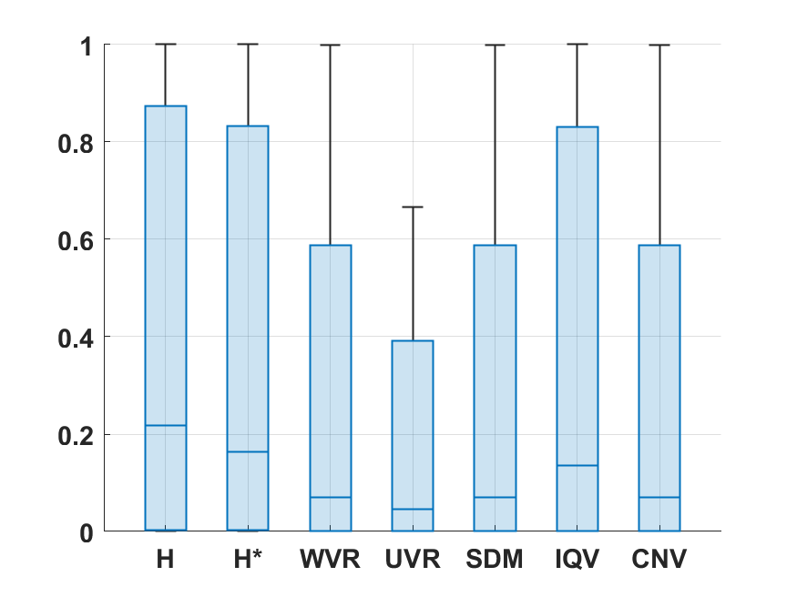
Figure 7: Box and whisker plot of uncertainty statistics for AF classifier.

5 Conclusion

In this paper, we have presented a metrological framework for evaluating uncertainty within machine learning classification models, motivated by the increasing use of classification models in a wide range of applications. We have identified and listed a number of sources of uncertainty within ML classification models which contribute to the output predictive uncertainty of the nominal property or variable, namely training data uncertainty, class assignment uncertainty, uncertainty about choice of model, model parameter uncertainty, and input data uncertainty, only some of which are currently addressed in the GUM suite of documents.

The work described in this paper has focused primarily on predictive uncertainty of ML classification models, with a specific focus on probabilistic ML classification models, i.e. models that return class probabilities for the output nominal variable. This focus included the evaluation of uncertainty for such nominal variables, which is not currently considered within the VIM and GUM. We have demonstrated that the PMF provides a complete characterisation of the uncertainty associated with nominal properties, and thus the predictive uncertainty in probabilistic ML classifiers. We have also motivated the use of the PMF of a nominal variable, as opposed to a summary statistic, in propagating such uncertainty within a chain of measurement models, representing either a metrological traceability chain or a processing chain for information products. We then provided example approaches using analytic or sampling methods of how to perform such propagation using the PMF.

We have reviewed various statistics that have been proposed within the literature associated with expressing the predictive uncertainty of probabilistic ML classifiers. We provided a comparison between these statistics in terms of their fundamental properties, and applied them in the context of two case studies that rely upon a metrological analysis, namely land cover classification, and atrial fibrillation detection. We found that for both case studies, the information entropy, which is the most common statistic for uncertainty within the ML community, is the most sensitive to variations in the predictive probability distributions. We have also illustrated how sources of uncertainty are addressed within the two case studies using different methodologies dependent on the classification modelling procedure.

The framework we have outlined builds upon and enhances previous work in uncertainty evaluation for nominal properties. The framework enables an extension of the VIM and GUM to uncertainty evaluation for nominal properties, and provides methods for handling the sources of uncertainty within ML classification, underpinning their use within metrological applications.

Funding

This work was funded by the UK Government’s Department for Science, Innovation and Technology (DSIT) through the UK’s National Measurement System (NMS) programmes. Anna Pustogvar’s work was also supported by a College of Science and Engineering (CSE) Scholarship from the University of Leicester.

Data Sources

The original data used for LC classification study can be found at [81, 82, 83, 84]. More details on how this data was processed for the LC classification study are provided in [14]. The original data for the case study on AF detection (DeepBeat) can be found at [85] and is described in [9]. The custom data split used was described in [74].

References

- [1] BIPM et al. “International Vocabulary of Metrology — Basic and general concepts and associated terms (VIM)”, Joint Committee for Guides in Metrology, JCGM 200:2012. (3rd edition) DOI: https://doi.org/10.59161/JCGM200-2012
- [2] BIPM et al. “Evaluation of measurement data — Guide to the expression of uncertainty in measurement”, Joint Committee for Guides in Metrology, JCGM 100:2008 DOI: https://doi.org/10.59161/JCGM100-2008E
- [3] ESA “HR_LandCover_CCI+ - Phase 1. D2.2. Algorithm Theoretical Basis Document (ATBD)”, 2022 URL: https://climate.esa.int/media/documents/CCI_HRLC_Ph1-D2.2_ATBD_v4.0.pdf
- [4] ESA “Lakes_CCI+ - Phase 2. D2.2. Algorithm Theoretical Basis Document (ATBD)”, 2023 URL: https://climate.esa.int/media/documents/Lakes_CCI_D2-2_ATBD.pdf
- [5] Sergii Skakun et al. “Cloud Mask Intercomparison eXercise (CMIX): An evaluation of cloud masking algorithms for Landsat 8 and Sentinel-2” In Remote Sensing of Environment 274, 2022 DOI: https://doi.org/10.1016/j.rse.2022.112990
- [6] Jeroen Buters et al. “Automatic detection of airborne pollen: an overview” Publisher: Springer Science and Business Media LLC In Aerobiologia 40.1, 2024, pp. 13–37 DOI: 10.1007/s10453-022-09750-x
- [7] Sophie Erb et al. “Real-time pollen identification using holographic imaging and fluorescence measurements” Publisher: Copernicus GmbH In Atmospheric Measurement Techniques 17.2, 2024, pp. 441–451 DOI: 10.5194/amt-17-441-2024
- [8] Jenny Venton et al. “Robustness of convolutional neural networks to physiological electrocardiogram noise” In Philosophical Transactions of the Royal Society A 379.2212, 2021, pp. 20200262
- [9] Jessica Torres-Soto and Euan A Ashley “Multi-task deep learning for cardiac rhythm detection in wearable devices” In NPJ digital medicine 3.1, 2020, pp. 116
- [10] Sebastian Heidenreich et al. “Strategic Agenda, European Metrology Network for Mathematics and Statistics” EURAMET, 2023, pp. 1–68 URL: https://www.euramet.org/european-metrology-networks/mathmet/strategy/strategic-research-agenda
- [11] Emma Woolliams “A metrological framework for addressing uncertainty in satellite and in situ Earth environmental observations” Submitted, 2025
- [12] Eyke Hüllermeier and Willem Waegeman “Aleatoric and epistemic uncertainty in machine learning: An introduction to concepts and methods” In Machine learning 110.3, 2021, pp. 457–506
- [13] Kevin P Murphy “Machine learning: a probabilistic perspective” MIT press, 2012
- [14] Samuel Bilson and Anna Pustogvar “Uncertainty-aware Bayesian machine learning modelling of land cover classification”, 2025 arXiv: https://arxiv.org/abs/2503.21510
- [15] Yarin Gal and Zoubin Ghahramani “Dropout as a Bayesian Approximation: Representing Model Uncertainty in Deep Learning” arXiv:1506.02142 arXiv, 2016 DOI: 10.48550/arXiv.1506.02142
- [16] Alex Kendall and Yarin Gal “What uncertainties do we need in bayesian deep learning for computer vision?” In Advances in neural information processing systems 30, 2017
- [17] Trevor Hastie, Robert Tibshirani and Jerome Friedman “The Elements of Statistical Learning. Data Mining, Inference, and Prediction” Springer, 2008
- [18] BIPM et al. “Evaluation of measurement data — Supplement 1 to the “Guide to the expression of uncertainty in measurement” — Propagation of distributions using a Monte Carlo method”, Joint Committee for Guides in Metrology, JCGM 101:2008 DOI: https://doi.org/10.59161/JCGM101-2008
- [19] BIPM et al. “Evaluation of measurement data — Supplement 2 to the “Guide to the expression of uncertainty in measurement” — Extension to any number of output quantities”, Joint Committee for Guides in Metrology, JCGM 102:2011 DOI: https://doi.org/10.59161/jcgm102-2011
- [20] BIPM et al. “Guide to the expression of uncertainty in measurement — Part 6: Developing and using measurement models”, Joint Committee for Guides in Metrology, JCGM GUM-6:2020 DOI: https://doi.org/10.59161/jcgmgum-6-2020
- [21] BIPM et al. “Evaluation of measurement data — The role of measurement uncertainty in conformity assessment”, Joint Committee for Guides in Metrology, JCGM 106:2012 DOI: https://doi.org/10.59161/jcgm106-2012
- [22] J. Louis and L2A team “Sentinel-2 Level-2A Algorithm Theoretical Basis Document”, 2021 URL: https://step.esa.int/thirdparties/sen2cor/2.10.0/docs/S2-PDGS-MPC-L2A-ATBD-V2.10.0.pdf
- [23] Dan López-Puigdollers, Gonzalo Mateo-García and Luis Gómez-Chova “Benchmarking Deep Learning Models for Cloud Detection in Landsat-8 and Sentinel-2 Images” In Remote Sensing 13.992, 2021 DOI: 10.3390/rs13050992
- [24] Ricardo Bettencourt da Silva and Stephen L.. Ellison “Eurachem/CITAC Guide: Assessment of performance and uncertainty in qualitative chemical analysis” In Eurachem, 2021 URL: https://www.eurachem.org/index.php/publications/guides/performance-and-uncertainty-in-qualitative-analysis
- [25] Gunnar Nordin, René Dybkaer, Urban Forsum and Xavier Fuentes-Arderiu “Vocabulary on nominal property, examination, and related concepts for clinical laboratory sciences (IFCC-IUPAC Recommendations 2017)” In Pure and Applied Chemistry 90.5, 2018, pp. 913–935 DOI: https://doi.org/10.1515/pac-2011-0613
- [26] S.. Stevens “On the Theory of Scales of Measurement” Publisher: American Association for the Advancement of Science In Science 103.2684, 1946, pp. 677–680 URL: https://www.jstor.org/stable/1671815
- [27] Rod White “The meaning of measurement in metrology” In Accreditation and Quality Assurance 16.1, 2011, pp. 31–41 DOI: 10.1007/s00769-010-0698-1
- [28] F. Mosteller and J.. Tukey “Data Analysis and Regression: A Second Course in Statistics” Addison-Wesley Pub Co, 1977
- [29] “ISO 33406:2024 Approaches for the production of reference materials with qualitative properties” First edition, 2024
- [30] Alan Agresti “Categorical Data Analysis”, Wiley Series in Probability and Statistics Hoboken, NJ: Wiley, 2002
- [31] Luca Mari, Claudio Narduzzi, Gunnar Nordin and Stefanie Trapmann “Foundations of uncertainty in evaluation of nominal properties” In Measurement 152, 2020, pp. 107397 DOI: https://doi.org/10.1016/j.measurement.2019.107397
- [32] Luca Mari “Toward a harmonized treatment of nominal properties in metrology” In Metrologia 54, 2017, pp. 784–795 DOI: https://doi.org/10.1088/1681-7575/aa8521
- [33] Antonio Possolo et al. “A brief guide to measurement uncertainty (IUPAC Technical Report)” In Pure and Applied Chemistry 96.1, 2024, pp. 113–134 DOI: https://doi.org/10.1515/pac-2022-1203
- [34] “ISO/IEC 17025 General requirements for the competence of testing and calibration laboratories” Third edition, 2017
- [35] Antonio Possolo “Simple Guide for Evaluating and Expressing the Uncertainty of NIST Measurement Results”, 2015 DOI: 10.6028/NIST.TN.1900
- [36] BIPM et al. “Guide to the expression of uncertainty in measurement — Part 1: Introduction”, Joint Committee for Guides in Metrology, JCGM GUM-1:2023 DOI: https://doi.org/10.59161/jcgmgum-1-2023
- [37] Allen R. Wilcox “Indices of Qualitative Variation and Political Measurement” Publisher: [University of Utah, Sage Publications, Inc., Western Political Science Association] In The Western Political Quarterly 26.2, 1973, pp. 325–343 DOI: 10.2307/446831
- [38] Shervin Shirmohammadi, Mohammad Hadi Amiri and Hussein Al Osman “Measurement Methodology: Uncertainty as a Predictor of Classification Accuracy in Machine Learning-Assisted Measurements” Conference Name: IEEE Instrumentation & Measurement Magazine In IEEE Instrumentation & Measurement Magazine 27.7, 2024, pp. 37–45 DOI: 10.1109/MIM.2024.10700740
- [39] Tarald O. Kvålseth “Variation for Categorical Variables” In International Encyclopedia of Statistical Science Berlin, Heidelberg: Springer, 2011, pp. 1642–1645 DOI: 10.1007/978-3-642-04898-2˙608
- [40] Patrick Bogaert, François Waldner and Pierre Defourny “An information-based criterion to measure pixel-level thematic uncertainty in land cover classifications” In Stochastic Environmental Research and Risk Assessment 31.9, 2017, pp. 2297–2312 DOI: 10.1007/s00477-016-1310-y
- [41] C.. Shannon “A mathematical theory of communication” Conference Name: The Bell System Technical Journal In The Bell System Technical Journal 27.3, 1948, pp. 379–423 DOI: 10.1002/j.1538-7305.1948.tb01338.x
- [42] Antonio Possolo “Statistical models and computation to evaluate measurement uncertainty” In Metrologia 51, 2014, pp. 228–236 DOI: https://doi.org/10.1088/0026-1394/51/4/S228
- [43] Edwin T. Jaynes “Prior Probabilities” Conference Name: IEEE Transactions on Systems Science and Cybernetics In IEEE Transactions on Systems Science and Cybernetics 4.3, 1968, pp. 227–241 DOI: 10.1109/TSSC.1968.300117
- [44] N.R. Pal and J.C. Bezdek “Measuring fuzzy uncertainty” Conference Name: IEEE Transactions on Fuzzy Systems In IEEE Transactions on Fuzzy Systems 2.2, 1994, pp. 107–118 DOI: 10.1109/91.277960
- [45] F. Löw, U. Michel, S. Dech and C. Conrad “Impact of feature selection on the accuracy and spatial uncertainty of per-field crop classification using Support Vector Machines” In ISPRS Journal of Photogrammetry and Remote Sensing 85, 2013, pp. 102–119 DOI: 10.1016/j.isprsjprs.2013.08.007
- [46] Patrick Bogaert, François Waldner and Pierre Defourny “An Information-Based Criterion to Measure Pixel-Level Thematic Uncertainty in Land Cover Classifications” In Stochastic Environmental Research and Risk Assessment 31.9, 2017, pp. 2297–2312 DOI: 10.1007/s00477-016-1310-y
- [47] Jose Rubia “Measures of Variability for Qualitative Variables Using the R Software” Number: 3 Publisher: Scientific Research Publishing In Open Journal of Statistics 14.3, 2024, pp. 259–293 DOI: 10.4236/ojs.2024.143013
- [48] Tarald O. Kvålseth “Measuring variation for nominal data” In Bulletin of the Psychonomic Society 26.5, 1988, pp. 433–436 DOI: 10.3758/BF03334906
- [49] Paul Glasziou and Jørgen Hilden “Test Selection Measures” Publisher: SAGE Publications Inc STM In Medical Decision Making 9.2, 1989, pp. 133–141 DOI: 10.1177/0272989X8900900208
- [50] Tarald O. Kvålseth “Coefficients of Variation for Nominal and Ordinal Categorical Data” Publisher: SAGE Publications Inc In Perceptual and Motor Skills 80.3, 1995, pp. 843–847 DOI: 10.2466/pms.1995.80.3.843
- [51] Timothy A. Sipkens, Joel C. Corbin, Samuel J. Grauer and Gregory J. Smallwood “Tutorial: Guide to error propagation for particle counting measurements” In Journal of Aerosol Science 167, 2023, pp. 106091 DOI: 10.1016/j.jaerosci.2022.106091
- [52] Theodore J. Bohn and Enrique R. Vivoni “MOD-LSP, MODIS-based Parameters for Hydrologic Modeling of North American Land Cover Change” In Scientific Data 6.1, 2019 DOI: 10.1038/s41597-019-0150-2
- [53] Libo Wang et al. “Mapping of ESA’s Climate Change Initiative Land Cover Data to Plant Functional Types for Use in the CLASSIC Land Model” In Biogeosciences 20.12, 2023, pp. 2265–2282 DOI: 10.5194/bg-20-2265-2023
- [54] IPCC “Guidelines for National Greenhouse Gas Inventories”, 2006
- [55] Andrew K. Skidmore et al. “Priority List of Biodiversity Metrics to Observe from Space” In Nature Ecology & Evolution 5.7, 2021, pp. 896–906 DOI: 10.1038/s41559-021-01451-x
- [56] A.M. Kilcoyne et al. “Living England: Satellite Based Habitat Classification. Technical User Guide”, 2022
- [57] C. Marston, C.S. Rowland, A.W. O’Neil and R.D. Morton “Land Cover Map 2021 (10m Classified Pixels, GB)” NERC EDS Environmental Information Data Centre, 2022 DOI: 10.5285/a22baa7c-5809-4a02-87e0-3cf87d4e223a
- [58] Mark A. Friedl et al. “Medium Spatial Resolution Mapping of Global Land Cover and Land Cover Change Across Multiple Decades From Landsat” In Frontiers in Remote Sensing 3, 2022 DOI: 10.3389/frsen.2022.894571
- [59] Zander S. Venter and Markus A.. Sydenham “Continental-Scale Land Cover Mapping at 10 m Resolution Over Europe (ELC10)” In Remote Sensing 13.12, 2021 DOI: 10.3390/rs13122301
- [60] Christopher F. Brown et al. “Dynamic World, Near Real-Time Global 10 m Land Use Land Cover Mapping” In Scientific Data 9.1, 2022 DOI: 10.1038/s41597-022-01307-4
- [61] Krishna Karra et al. “Global Land Use / Land Cover with Sentinel 2 and Deep Learning” In 2021 IEEE International Geoscience and Remote Sensing Symposium IGARSS Brussels, Belgium: IEEE, 2021, pp. 4704–4707 DOI: 10.1109/IGARSS47720.2021.9553499
- [62] Daniele Zanaga et al. “ESA WorldCover 10 m 2021 V200”, 2022 DOI: 10.5281/zenodo.7254221
- [63] EEA “CORINE Land Cover 2018 (raster 100 m)”, 2020 DOI: https://doi.org/10.2909/960998c1-1870-4e82-8051-6485205ebbac
- [64] Daniel Moraes, Manuel L. Campagnolo and Mário Caetano “Training Data in Satellite Image Classification for Land Cover Mapping: A Review” In European Journal of Remote Sensing 57.1, 2024 DOI: 10.1080/22797254.2024.2341414
- [65] Laurent Valentin Jospin et al. “Hands-on Bayesian Neural Networks – a Tutorial for Deep Learning Users” arXiv:2007.06823 arXiv, 2022 DOI: 10.48550/arXiv.2007.06823
- [66] Luca Franceschi et al. “Hyperparameter Optimization in Machine Learning”, 2024 arXiv: https://arxiv.org/abs/2410.22854
- [67] Jasper Snoek, Hugo Larochelle and Ryan P Adams “Practical Bayesian Optimization of Machine Learning Algorithms” In Advances in Neural Information Processing Systems 25 Curran Associates, Inc., 2012 URL: https://proceedings.neurips.cc/paper_files/paper/2012/file/05311655a15b75fab86956663e1819cd-Paper.pdf
- [68] Rui Tuo and Wenjia Wang “Uncertainty Quantification for Bayesian Optimization” In Proceedings of The 25th International Conference on Artificial Intelligence and Statistics 151, Proceedings of Machine Learning Research PMLR, 2022, pp. 2862–2884 URL: https://proceedings.mlr.press/v151/tuo22a.html
- [69] Steve Brooks, Andrew Gelman, Galin Jones and Xiao-Li Meng “Handbook of Markov Chain Monte Carlo” CRC press, 2011
- [70] Tilmann Gneiting and Adrian E Raftery “Strictly proper scoring rules, prediction, and estimation” In Journal of the American statistical Association 102.477 Taylor & Francis, 2007, pp. 359–378
- [71] Luciana Ferrer “Analysis and Comparison of Classification Metrics” arXiv:2209.05355 arXiv, 2023 DOI: 10.48550/arXiv.2209.05355
- [72] S… Du Toit, A… Steyn and R.. Stumpf “Graphical Exploratory Data Analysis”, Springer Texts in Statistics New York, NY: Springer, 1986 DOI: 10.1007/978-1-4612-4950-4
- [73] Dominik Linz et al. “Atrial fibrillation: epidemiology, screening and digital health” In The Lancet Regional Health–Europe 37, 2024
- [74] Ciaran Bench et al. “Towards Trustworthy Atrial Fibrillation Classification From Wearables Data: Quantifying Model Uncertainty” In Computing in Cardiology, 2024
- [75] Femke Wouters et al. “Comparative evaluation of consumer wearable devices for atrial fibrillation detection: A validation study (Preprint)” In JMIR Formative Research, 2024 URL: https://api.semanticscholar.org/CorpusID:274172555
- [76] “Fibricheck: Advanced heart rhythm monitoring for detection and management of atrial fibrillation” Accessed: 31-12-2024, https://www.fibricheck.com/
- [77] Peter H Charlton et al. “Wearable photoplethysmography for cardiovascular monitoring” In Proceedings of the IEEE 110.3, 2022, pp. 355–381
- [78] Nils Strodthoff, Patrick Wagner, Tobias Schaeffter and Wojciech Samek “Deep Learning for ECG Analysis: Benchmarks and Insights from PTB-XL” In IEEE Journal of Biomedical and Health Informatics 25.5, 2020, pp. 1519–1528
- [79] Tong He et al. “Bag of tricks for image classification with convolutional neural networks” In Proceedings of the IEEE/CVF conference on computer vision and pattern recognition, 2019, pp. 558–567
- [80] J. Martin and C. Elster “Aleatoric Uncertainty for Errors-in-Variables Models in Deep Regression” In Neural Processing Letters 55.4, 2023, pp. 4799–4818
- [81] R.D. Morton, C.G. Marston, A.W. O’Neil and C.S. Rowland “Land Cover Map 2017 (20m classified pixels, GB)” NERC Environmental Information Data Centre, 2020 DOI: https://doi.org/10.5285/f6f86b1a-af6d-4ed8-85af-21ee97ec5333
- [82] R.D. Morton, C.G. Marston, A.W. O’Neil and C.S. Rowland “Land Cover Map 2018 (20m classified pixels, GB)” NERC Environmental Information Data Centre, 2020 DOI: https://doi.org/10.5285/b3dfc4c7-c9bd-4a02-bed8-46b2a41be04a
- [83] R.D. Morton, C.G. Marston, A.W. O’Neil and C.S. Rowland “Land Cover Map 2019 (20m classified pixels, GB)” NERC Environmental Information Data Centre, 2020 DOI: https://doi.org/10.5285/643eb5a9-9707-4fbb-ae76-e8e53271d1a0
- [84] R.D. Morton, C.G. Marston, A.W. O’Neil and C.S. Rowland “Land Cover Map 2020 (10m classified pixels, GB)” NERC EDS Environmental Information Data Centre, 2021 DOI: https://doi.org/10.5285/35c7d0e5-1121-4381-9940-75f7673c98f7
- [85] Jessica Torres-Soto and Euan A Ashley “DeepBeat”, https://github.com/AshleyLab/deepbeat