Non-stabilizerness and violations of CHSH inequalities

Abstract

We study quantitatively the interplay between entanglement and non-stabilizer resources in violating the CHSH inequalities. We show that, while non-stabilizer resources are necessary, they must have a specific structure, namely they need to be both asymmetric and (surprisingly) local. We employ stabilizer entropy (SE) to quantify the non-stabilizer resources involved and the probability of violation given the resources. We show how spectral quantities related to the flatness of entanglement spectrum and its relationship with non-local SE affect the CHSH inequality. Finally, we utilize these results - together with tools from representation theory - to construct a systematic way of building ensembles of states with higher probability of violation.

1 Introduction

It is a well-known fact that the Clauser-Horne-Shimony-Holt (CHSH) inequality [1] can be violated in quantum mechanics due to quantum entanglement. However, it has been recognized more recently that entanglement alone is not sufficient: resources beyond stabilizerness - colloquially known as magic - are also necessary [2, 3, 4, 5].

In this paper, we perform a theoretical and quantitative study of the interplay between the entangling and non-stabilizer resources necessary to violate the CHSH inequalities. To this end, we build a setting that does not arbitrarily separate the resources involved in state preparation and measurement.

Non-stabilizer resources are also necessary together with entanglement to attain a quantum advantage [6, 7, 8]. Recently, it has been put forward the notion that other features of quantum complexity require both entangling and non-stabilizer resources [9, 10]. In order to quantify non-stabilizerness, we resort to the Stabilizer Entropy (SE), the unique computable monotone of non-stabilizerness for pure states [11, 12]. SE is experimentally measurable [13] and efficiently computable by tensor networks methods [14, 15, 16]. Having a computable quantity such as SE at disposal, has allowed to test and quantify the role of non-stabilizer resources in several settings and scenarios, ranging from quantum phase transitions [17, 18, 19, 20, 21] and quantum chaos [10, 22, 23], to high-energy physics [24, 25, 26, 27], quantum-information [28, 29, 30, 31, 32, 33, 34, 35, 36, 9, 37, 38], and condensed matter [39, 40, 41, 42, 43, 44, 45, 46, 47, 48, 49, 50].

In this paper, we detail what kind of structure entanglement and SE need to have in order to violate the CHSH inequality. Counterintuitively, we prove that SE needs to be local in order to obtain a violation: non-local SE [24] is shown to be detrimental to CHSH violations. Moreover, the resources must be asymmetric between Alice and Bob. We use both Haar averaging and numerical techniques to compute the probability of violations given the resources. Finally, we use the technique of isospectral twirling to show how knowledge of the structure of entangling and non-stabilizer resources can be used to improve the probability of a CHSH violation when one lacks perfect control of the system.

2 Setting

The seminal work of the Horodecki’s [51] establishes necessary and sufficient conditions on the state preparation in order to violate CHSH inequalities by means of local measurements. However, it was noted in [2] that one would need non-Clifford measurements. Because of the state-effect duality, though, it is clear that one could just perform measurements that are neutral from the stabilizer resources point of view if one prepares the state with the required resources. Let us make an example. Define the CHSH operator (we omit the tensor product symbol when not strictly necessary)

$$B_{0}:=X\otimes(X+Z)+Z\otimes(-X+Z)=XX+XZ-ZX+ZZ\,.$$ (1)

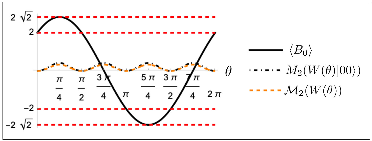
Figure 1: Plot of the expectation value of the rotated operator $\langle B_{0}\rangle$ (solid black line), the SE $M_{2}$ of the rotated Bell state $W(\theta)\ket{00}$ (dashed-dotted black line) and the non-stabilizing power $\mathcal{M}_{2}$ of the rotation operator (dashed orange line). The dashed red lines represent the values of violation of CHSH inequalities and the Tsirelson’s bound.

The above operator is short-hand to describe four measurements that are both local and within the stabilizer formalism, being Pauli measurements. It is immediately clear that, even preparing a Bell state (say $\ket{\Phi^{+}}=\frac{\ket{00}+\ket{11}}{\sqrt{2}}$), these measurements will not lead to a CHSH violation, as $\Tr(B_{0}\Phi^{+})=2$. On the other hand, if we prepare the state $R_{y}(\theta)\otimes I\ket{\Phi^{+}}=\exp[-i\frac{\theta}{2}Y]\otimes I\ket{\Phi^{+}}=(R_{y}(\theta)\otimes I)C_{X}(H\otimes I)\ket{00}\equiv W(\theta)\ket{00}$ one can violate the CHSH inequalities for a certain range of the rotation angle $\theta$, see Fig. 1. As one can see, it is possible to use non-Clifford resources to prepare the state $W(\theta)\ket{00}$. A direct computation of the SE gives ${M}_{2}(W(\theta)\ket{00})=-\log\left[{7+\cos(4\theta)}/{8}\right]$ (see Eq. (3) below for a definition of $M_{2}$). Of course, what we just did is equivalent to preparing the state $\Phi^{+}$ and using the CHSH operator $R^{\dagger}_{y}(\theta)B_{0}R_{y}(\theta)$. Notice that the Tsirelson’s bound, $\left|\Tr(B_{0}\psi)\right|\leq 2\sqrt{2}$, is saturated for the state $W(\pi/4)\ket{00}$ for which $M_{2}$ has a maximum, see Fig. 1. This simple example shows that, in order to address the resources needed for a task, one has to initialize the system in a resource-free state, from now on $\omega_{0}:=\ket{00}\bra{00}$ and perform resource-free measurements. Since for a single qubit the only Clifford measurements are along $\{X,Y,Z\}$, we must consider out of the general two-qubit CHSH operators, only the subset ${\mathcal{B}}=\{B|B=P_{A}\otimes(P_{B}+P_{B^{\prime}})+P_{A^{\prime}}\otimes(P_{B}-P_{B^{\prime}}),$ with $P_{A,B,A^{\prime},B^{\prime}}\in\{X,Y,Z\}\}$. Note that $\mathcal{B}$ coincides with the set $\{C_{A}^{\dagger}\otimes C_{B}^{\dagger}B_{0}C_{A}\otimes C_{B}\}$ where $C_{A},C_{B}\in\mathcal{C}$ are single-qubit Clifford unitaries. All the resources are then injected by the state preparation $U$ (in case of unitary preparation): $\omega_{0}\mapsto\omega_{U}\equiv U\omega_{0}U^{\dagger}$ and the central object of our study, the expectation value of the resource-free CHSH operator $B$, reads

$$b_{U}:=\Tr[B\omega_{U}]\equiv\Tr[B_{U}\omega_{0}]$$ (2)

We see that all the resources needed for the task have been inserted in $U$. In the following, we study how both non-stabilizer and entanglement resources need to be encoded in $U$ in order to violate the CHSH inequality $|b_{U}|\leq 2$.

3 Stabilizer Entropy

Consider a system of $n$ qubits and the set of Pauli strings $\mathbb{P}_{n}=\{{I},X,Y,Z\}^{\otimes n}$. For a pure state $\ket{\psi}$ and $P\in\mathbb{P}_{n}$, the quantity $\Xi_{P}(\ket{\psi}):=d^{-1}(\Tr{P\psi})^{2}$ is a probability distribution over $\mathbb{P}_{n}$, with $d=2^{n}$. The $2$-SE $M_{2}(\ket{\psi})$ is defined as the (shifted) $2-$Rényi entropy

$$M_{2}(\ket{\psi}) := -\log\left[d\sum_{P\in\mathbb{P}_{n}}\Xi_{P}(\psi)^{2}\right]=-\log\left(d^{-1}\sum_{P\in\mathbb{P}_{n}}\Tr^{4}[\psi P]\right)=-\log d\Tr[Q\outerproduct{\psi}{\psi}^{\otimes 4}]$$ (3)

where $Q:=d^{-2}\sum_{P\in\mathbb{P}_{n}}P^{\otimes 4}$. The 2-SE can be extended to generic mixed states by $\tilde{M}_{2}(\rho)=M_{2}(\rho)-S_{2}(\rho)$, where $S_{2}(\rho)=-\log\Tr[\rho^{2}]$ is the 2-Rényi entropy of $\rho$. Notice that $\chi$ is a free state, $\tilde{M}_{2}(\chi)=0$, if and only if $\chi=\frac{1}{d}\sum_{P\in\mathcal{G}}\phi_{P}P$, where $\mathcal{G}$ is an Abelian subgroup of the Pauli group $\mathcal{P}_{n}\equiv\mathbb{P}_{n}\times\{\pm 1,\pm i\}$ and $\phi_{P}=\pm 1$. The 2-SE $\tilde{M}_{2}$ is a good monotone for pure states [12], faithful with respect to the free states, invariant under Clifford unitaries and additive under tensor product, i.e. $\tilde{M}_{2}(\rho\otimes\sigma)=\tilde{M}_{2}(\rho)+\tilde{M}_{2}(\sigma)$.

Starting from the SE, one can define the 2 non-stabilizing power of a unitary $U$ as the average 2-SE created by the action of $U$ on the orbit of stabilizer states:

$$\mathcal{M}_{2}(U)=\frac{1}{|\rm{STAB}|}\sum_{\ket{\psi}\in\rm{STAB}}M_{2}(U\ket{\psi})\ .$$ (4)

For example, the non-stabilizing power of $W(\theta)$ is

$$\mathcal{M}_{2}(W(\theta))=-\frac{4}{5}\log\left(\frac{7+\cos(4\theta)}{8}\right)$$ (5)

In Fig. 1 we see how the magic power of $W(\theta)$ follows closely the magic of the state $W(\theta)|00\rangle$. Moreover the maximal CHSH violations coincide with maxima of $M_{2}$ and $\mathcal{M}_{2}$.

A related quantity to measure the interplay between SE and entanglement is the so called non-local non-stabilizerness [52] first introduced in [24]. Given a bipartition $AB$ of the Hilbert space, the non-local non-stabilizerness $M_{\rm NL}$ is defined as:

$$M_{\rm NL}(\ket{\psi})=\min_{U_{A}\otimes U_{B}}M_{2}(U_{A}\otimes U_{B}\ket{\psi})$$ (6)

This quantity measures the amount of non-stabilizerness that is non-local, i.e. that it cannot be erased from the state by means of local unitaries. As a consequence of the minimization procedure, non-local non stabilizerness is solely dependent on the entanglement spectrum, and in [52] an explicit expression for two qubit states is found: for any pure state $\ket{\psi}$ with entanglement spectrum $\{\cos^{2}(\theta),\sin^{2}(\theta)\}$, the non-local magic reads

$$M_{\rm NL}(\ket{\psi})=-\log\left(\frac{7+\cos(8\theta)}{8}\right)\;\ .$$ (7)

The state such that $M_{\rm NL}(\ket{\psi})=M_{2}(\ket{\psi})$ is $\ket{r(\theta)}=\cos(\theta)\ket{00}+\sin(\theta)\ket{11}$ modulo local Clifford unitaries.

4 Non-stabilizerness and violations of the CHSH inequality

In this section, we show some facts about the structure of entanglement and SE in the context the CHSH inequality. Informally, we show that in order to violate the CHSH inequality i) both entanglement and SE are necessary; ii) the preparation unitary $U$ must be asymmetric; iii) non-local magic hinders the violation of locality (!); and iv) probes of the interplay between entanglement and SE, like the capacity of entanglement, offer a valuable insight on the nature of the violation (or lack thereof).

Let us start by showing that $U$ must be both entangling and non-Clifford in order to violate CHSH. We indicate with $\mathcal{C}$ the Clifford group (the normalizer of the Pauli group).

Theorem 1.

Given an operator $B=P_{A}\otimes(P_{B}+P_{B^{\prime}})+P_{A^{\prime}}\otimes(P_{B}-P_{B^{\prime}})$ with $P_{A,B,A^{\prime},B^{\prime}}\in\{X,Y,Z\}$, a state $\omega_{0}=\outerproduct{00}{00}$ and a unitary Clifford operator $C\in\mathcal{C}$, then:

$$|{\rm Tr}\left[BC\omega_{0}C^{\dagger}\right]|\leq 2$$ (8)

Moreover, the same holds for mixed stabilizer states $\chi$ (obtained by convex combinations of pure stabilizer states): $|{\rm Tr}\left[B\chi\right]|\leq 2$.

Proof.

We say that the operator $B$ is degenerate if at least two terms in $B$ are equal. One sees that if $B$ is degenerate, then it is of the form $B=2P_{A}\otimes P_{B}$ and the result is obvious since $\|B_{0}\|=2$ in this case and $\left|\Tr(B_{0}\psi)\right|\leq\|B_{0}\|$ for all states $\psi$. Hence, we can assume that $B$ is non-degenerate ($A\neq A^{\prime}$ and $B\neq B^{\prime}$). To prove the first statement of the theorem, let us first note that $\psi=C\omega_{0}C^{\dagger}$ is a pure stabilizer state and so is of the form

$$\psi=\frac{1}{4}\sum_{P\in\mathcal{G}}\phi_{P}P$$ (9)

where $\mathcal{G}$ is an abelian subgroup of the Pauli group of dimension four and $\phi_{P}=\pm 1$. Now note that $B$ is a sum of four Pauli strings. Using orthogonality of Pauli strings ${\rm Tr}\left[PP^{\prime}\right]=d\delta_{PP^{\prime}}$, we obtain

$$b_{C}={\rm Tr}\left[BC\omega_{0}C^{\dagger}\right]=\phi_{P_{AB}}+\phi_{P_{AB^{\prime}}}+\phi_{P_{A^{\prime}B}}-\phi_{P_{A^{\prime}B^{\prime}}}\ .$$ (10)

At this point note that there can be at most two Pauli strings in $B$ commuting with each other and thus belonging to the same Abelian subgroup. To see this, note that when $B$ is non-degenerate ($A\neq A^{\prime}$ and $B\neq B^{\prime}$), $P_{A}\otimes P_{B}$ and $P_{A^{\prime}}\otimes P_{B^{\prime}}$ always commute (different Pauli operators anticommute) and any attempt to enlarge this set makes $B$ degenerate.

As a consequence, at most two terms in Eq. (10) can be different from zero, from which the theorem follows. As for the second part of the theorem, simply note that the if $\chi=\sum_{i}p_{i}\chi_{i}$ with $\chi_{i}$ pure stabilizer states and probabilities $p_{i}$ summing to one,

$$\left|\Tr[B\chi]\right|\leq\sum_{i}p_{i}\left|\Tr[B\chi_{i}]\right|\leq 2.$$ (11)

∎

Therefore, one cannot violate the CHSH inequality with either pure or mixed stabilizer states. Let us now show that if we restrict ourselves to the class of operators $B\in\mathcal{B}$ that we call symmetric, for which $P_{A}=P_{B}$ and $P_{A^{\prime}}=P_{B^{\prime}}$ (of which $B_{0}$ is an example) and the unitary preparation $U$ is symmetric in $A$ and $B$, there cannot be a violation either.

Theorem 2.

Given a unitary operator $U_{\rm sym}$ acting symmetrically on two qubits, that is, commuting with the swap operator $T_{2}$, then, for any symmetric resource free CHSH operator $B$

$$|{\rm Tr}\left[BU_{\rm sym}\omega_{0}U_{\rm sym}^{\dagger}\right]|\leq 2$$ (12)

Proof.

Let us first notice that any symmetric 2-qubit state, that is, it satisfies $T_{2}\ket{\psi}=\ket{\psi}$, can be written as a linear combination of the triplet states

$$\ket{\psi}=a\ket{00}+b\ket{11}+c\ket{\psi^{+}}$$ (13)

with $\ket{\psi^{+}}=\frac{\ket{01}+\ket{10}}{\sqrt{2}}$ and $|a|^{2}+|b|^{2}+|c|^{2}=1$. Now, since $[U_{\rm sym},T_{2}]=0$, the action of $U_{\rm sym}$ on a symmetric state is still a symmetric state and hence it has the same expression as Eq. (13). In particular then

$$U_{\rm sym}\ket{00}=a\ket{00}+b\ket{11}+c\ket{\psi^{+}}\,.$$ (14)

Direct evaluation of the expectation value of $B$ for symmetric resource free CHSH operators yields

$$\left|{\rm Tr}\left[BU_{\rm sym}\ket{00}\bra{00}U_{\rm sym}^{\dagger}\right]\right|=\Big{\{}2|c|^{2},|a+b|^{2},|a-b|^{2}\Big{\}}\leq 2\,,$$ (15)

where we used $\|\mathbf{x}\|_{1}\leq\sqrt{2}\|\mathbf{x}\|_{2}$ for $\mathbf{x}=(a,b)$. ∎

Let us finally move to our last theorem regarding non-locality and non-local non-stabilizerness. Since violations of the CHSH are connected with non-local behavior, one would naively expect non-local magic to play a major role in CHSH violations. It turns out that not only this is not the case, but it is actually the opposite: non-local magic is detrimental for the maximal violation of CHSH inequality. Indeed, one can prove that in presence of any amount of non-local non-stabilizerness it is not possible to saturate the Tsirelson bound. Conversely, it is necessary to have positive local non-stabilizerness in order to observe non-locality. For future convenience we introduce the local non-stabilizerness as the difference between the total $M_{2}$ and the non-local one:

$$M_{\rm LOC}(|\psi\rangle):=M_{2}(|\psi\rangle)-M_{\mathrm{NL}}(|\psi\rangle)\geq 0.$$ (16)

Theorem 3.

Given a state $\psi$ such that ${M}_{\rm NL}\neq 0$, then

$$\left|{\rm Tr}\left[B\psi\right]\right|<2\sqrt{2}$$ (17)

Moreover, if a unitary operator $U$ does not inject any local magic, that is $M_{\rm LOC}(U\ket{00})=0$, then

$$|b_{U}|=\left|{\rm Tr}\left[BU\omega_{0}U^{\dagger}\right]\right|\leq 2$$ (18)

Proof.

In order to achieve the Tsirelson’s bound [53], the state $\omega_{U}$ must be maximally entangled and in turn this means that

$$U\ket{00}=U_{A}\otimes U_{B}\frac{\ket{00}+\ket{11}}{\sqrt{2}}$$ (19)

which has zero non-local magic. This proves the first part of the statement.

If there is zero local magic, the state $U\ket{00}$ has the form [52]

$$U\ket{00} = C_{A}\otimes C_{B}({\cos\theta}\ket{00}+{\sin\theta}\ket{11})\equiv C_{A}\otimes C_{B}\ket{r(\theta)})$$ (20)

$$= \cos\theta\ket{ss^{\prime}}+\sin\theta\ket{\bar{s}\bar{s}^{\prime}}$$ (21)

where $\{\ket{s},\ket{\bar{s}}\}$ is a basis for Alice of eigenstates of Pauli operators and similarly for Bob, and $C_{A},C_{B}$ are local Clifford unitaries, which map $\ket{00}$ and $\ket{11}$ into the tensor product of eigenstates of other single qubit Pauli operators. Since $B=C_{A^{\prime}}^{\dagger}\otimes C_{B^{\prime}}^{\dagger}B_{0}C_{A^{\prime}}\otimes C_{B^{\prime}}$, it is sufficient to check the statement for $B_{0}$. One can then directly verify that for all possible combination of eigenstates of $\{X,Y,Z\}$ the inequality holds, proving the theorem. ∎

The detrimental effect of non-local magic on the maximal violation of the CHSH inequality can actually be quantified. More specifically, we claim that

$$\max_{U_{A}\otimes U_{B}}\left|{\rm Tr}\left[B_{U_{A}\otimes U_{B}}\outerproduct{r(\theta)}{r(\theta)}\right]\right|\leq 2\sqrt{2}-\frac{1}{2}M_{NL}(\ket{\psi}).$$ (22)

To show the above claim, we consider the function:

$$f_{U_{A},U_{B}}(\theta):=2\sqrt{2}-\frac{1}{2}M_{NL}(\theta)-\left|{\rm Tr}\left[B_{U_{A}\otimes U_{B}}\outerproduct{r(\theta)}{r(\theta)}\right]\right|$$ (23)

where $M_{\rm NL}(\theta)$ is defined in Eq. (6). In order to verify the claim we take 200 uniformly spaced values of $\theta\in[0,2\pi]$ and, for each of these, we sample uniformly $5\times 10^{5}$ Haar-random unitaries $U_{A}$, $U_{B}$, see Fig. 2. The shaded region represents the range of $f_{U_{A},U_{B}}(\theta)$, i.e. the maximum and minimum value taken by $f_{U_{A},U_{B}}(\theta)$ when sampling over $U_{A}\otimes U_{B}$. We observe that $f_{U_{A},U_{B}}(\theta)$ is always greater or equal than zero for all values of $\theta$, thus numerically supporting the inequality introduced in Eq. (22).

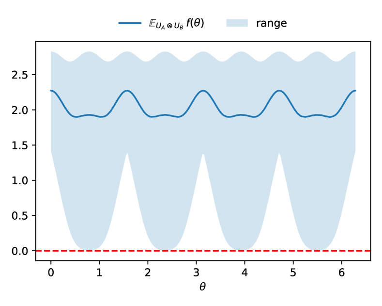
Figure 2: Average value and range of the function $f(\theta)=2\sqrt{2}-\frac{1}{2}M_{NL}(\theta)-\langle B\rangle_{\ket{\psi}}$ with $\theta\in[0,2\pi]$. For each of 200 uniformly spaced samples of $\theta$, $5\times 10^{5}$ Haar-random unitaries $U_{A}\otimes U_{B}$ were sampled. The curve represents the average value of $f(\theta)$ with respect to the sampled unitaries, while the shaded region indicates its range, i.e. the minimum and maximum values, at each sample of $\theta$. The absence of negative values from the range of $f(\theta)$ numerically supports the inequality in Eq. (22).

4.1 Probes of magic and non-locality

As we have seen, there is a very rich interplay between entanglement $E_{\mathrm{VN}}(|\psi\rangle)=S_{1}(\psi_{A})$, magic $M_{2}(\ket{\psi})$, non-local magic $M_{\rm NL}(|\psi\rangle)$, and the possibility of violation of CHSH inequality, and its maximum entity. Remarkably, non-local magic takes into account both entanglement and non-stabilizerness as factorized states have obviously zero non-local magic. As in general evaluating non-local magic is a daunting task, we also study the capacity of entanglement $C_{E}$ as a quantity that has some properties in common with it and can serve as a probe. $C_{E}(|\psi\rangle)$ is defined as

$$C_{E}(|\psi\rangle):=\left\langle(\log\psi_{A})^{2}\right\rangle_{\psi_{A}}-\left\langle\log\psi_{A}\right\rangle_{\psi_{A}}^{2}=\Tr\left[\psi_{A}\left(\log\psi_{A}\right)^{2}\right]-\left(\Tr[\psi_{A}\log\psi_{A}]\right)^{2}\,.$$ (24)

The entanglement capacity is a measure of how much the reduced state is non-flat, i.e. it measures how much $\psi_{A}$ deviates from being proportional to a projector [54, 55, 56]. Its connection with $M_{NL}$ is in the fact that $C_{E}(\psi=0)$ iff $\psi$ has zero non-local magic [24]. The $C_{E}$ has found applications in many-body systems, connecting thermodynamic quantities and the Rényi entropies [57, 58], and the AdS/CFT correspondence [59, 60, 24], where it has a relatively simple bulk interpretation given by metric fluctuations integrated over the Ryu-Takayanagi surface, i.e. the entangling surface.

Let us start with the family of states defined by

$$\ket{\rho} =\sqrt{\frac{r+1}{2}}\cos\left(\frac{\theta}{2}\right)\ket{00}-\sqrt{\frac{r+1}{2}}e^{-i\phi}\sin\left(\frac{\theta}{2}\right)\ket{01}$$

$$+\sqrt{\frac{r+1}{2}}e^{i\phi}\sin\left(\frac{\theta}{2}\right)\ket{10}+\sqrt{\frac{r+1}{2}}\cos\left(\frac{\theta}{2}\right)\ket{11},$$ (25)

with $r\in[0,1]$, $\theta\in[0,\pi]$ and $\phi\in[0,2\pi)$. The above state has the property that the reduced 1-qubit state $\rho_{A}$ is

$$\rho_{A}=\frac{I+\vec{r}\cdot\vec{\sigma}}{2}=\frac{1-r}{2}\ket{\rho_{-}}\bra{\rho_{-}}+\frac{1+r}{2}\ket{\rho_{+}}\bra{\rho_{+}}\,,$$ (26)

with $\vec{r}=r(\sin\theta\cos\phi,\sin\theta\sin\phi,\cos\theta)$, $\vec{\sigma}=(X,Y,Z)$ the vector of Pauli matrices and orthonormal vectors $|\rho_{\pm}\rangle$ given by

$$\ket{\rho_{+}} =\cos{\frac{\theta}{2}}\ket{0}+e^{i\phi}\sin{\frac{\theta}{2}}\ket{1}\,,$$ (27)

$$\ket{\rho_{-}} =\sin{\frac{\theta}{2}}\ket{0}-e^{i\phi}\cos{\frac{\theta}{2}}\ket{1}\,.$$ (28)

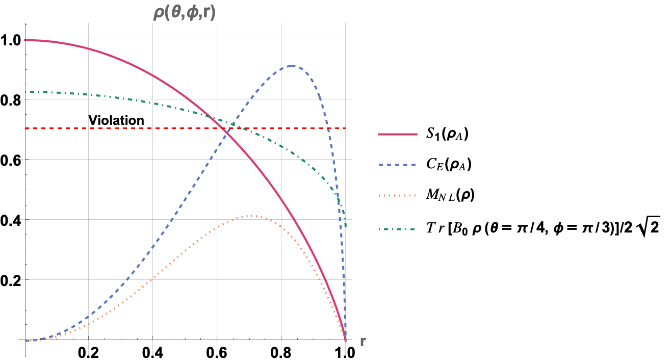
Figure 3: Plot of the entanglement entropy $S_{1}(\rho_{A})$ (magenta solid line), the capacity of entanglement $C_{E}(\rho_{A})$ (dashed indigo line), the non-local non-stabilizerness $M_{NL}(\rho)$ (dotted orange line) and of $\Tr[B_{0}\outerproduct{\rho}{\rho}]$ as a function of $r$, having set $\theta=\frac{\pi}{4}$ and $\phi=\frac{\pi}{3}$ (dotted-dashed green line). For $r=0$ the corresponding state is a combination of all four computational basis states, $M_{\rm NL}=0$ as well as $C_{E}$, while entanglement is maximum. Under these conditions, the CHSH inequality (dashed red line) is violated. One can then observe the decrease of the CHSH violation as $C_{E}$ and $M_{\rm NL}$ grow, up to a point where no violation is observed, in spite of the state being still highly entangled, as proven by the non-zero value of $S_{1}$. Finally, for $r=1$, both $M_{\rm NL}$ and $C_{E}$ are once again zero, but it is still not possible to violate the CHSH inequality because of the missing entanglement, since $S_{1}=0$.

Let us set $\theta=\pi/4$ and $\phi=\pi/3$ in Eq.(25) in order to have a state spanning all four computational basis states, and compute the quantities of interest to obtain

$$S_{1}(\rho_{A}) = \frac{1}{2}\log\left(\frac{4}{1-r^{2}}\right)-2r\frac{\text{arctanh}(r)}{\ln(4)}$$ (29)

$$C_{E}(\rho_{A}) = -\frac{\left(r^{2}-1\right)\log^{2}\left(\frac{2}{r+1}-1\right)}{4}\,$$ (30)

$$M_{\rm NL}(\outerproduct{\rho}{\rho}) = -\log(1-r^{2}+r^{4})$$ (31)

$${\rm Tr}\left[B_{0}\outerproduct{\rho}{\rho}\right] = \frac{3}{8}\left(2\sqrt{1-r^{2}}+\sqrt{2-2r^{2}}+2\sqrt{2}\right)\,,$$ (32)

The results are summarized in Fig. 3. First of all, we see how the qualitative similar trend (and same values at the boundaries) makes $C_{E}$ a good probe for $M_{\rm NL}$. Unfortunately, for two qubits they are not strictly monotone with each other. In this family one has maximal CHSH violation for $r=0$ while the non-local magic and the entanglement capacity are both zero. As $r$ grows, the expectation value of the Bell operator $B_{0}$ decreases, while the non-local magic increases, showing how non-local non-stabilizerness may hinder the violation of the CHSH inequality. Beyond a critical value of $r$, CHSH violations are not observed anymore, as there is too much non-local magic. Notice also that at the critical value of $r$ for which violations are not observed anymore, the state is still entangled, as shown by the entanglement entropy.

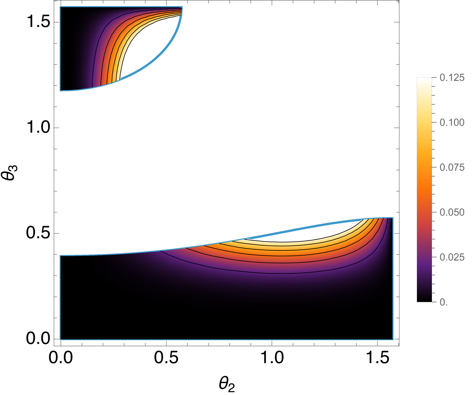
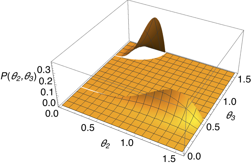
Figure 4: Density of states violating the CHSH inequality in the $\{\theta_{2},\theta_{3}\}$ plane. The region of violation of the Bell’s inequality. Left panel: density plot, the color code corresponds to the density of states in this chart. Right panel: 3D plot. Note that in these coordinates the maximal violation corresponds to the point $(\theta_{2},\theta_{3})=(0,\pi/2)$ and the line $(\theta_{2},\theta_{3})=(\theta,0)$ for $\theta\in[0,\pi/2]$.

4.2 CHSH geometry

Let us now try to get some geometric understanding regarding the region of pure states that violate the CHSH inequality. We start by going to the eigenbasis of the operator $B_{0}=\sum_{i}\lambda_{i}|\phi_{i}\rangle\langle\phi_{i}|,$ where we ordered the eigenvalues as $\lambda_{i}=\left\{-2\sqrt{2},2\sqrt{2},0,0\right\}$. A generic pure state $|\psi\rangle$ in this eigenbasis reads $|\psi\rangle=\sum_{i}\psi_{i}|\phi_{i}\rangle$. The condition $\left|\langle\psi|B_{0}|\psi\rangle\right|>2$ does not identify a vector subspace. Indeed, it can be rewritten as:

$$\left|\langle\psi|\left(\sum_{i}\lambda_{i}|\phi_{i}\rangle\langle\phi_{i}|\right)|\psi\rangle\right|>2\Leftrightarrow\left|\left(\sum_{i}\lambda_{i}\left|\psi_{i}\right|^{2}\right)\right|>2\Leftrightarrow\,\left|\left|\langle\phi_{1}|\psi\rangle\right|^{2}-\left|\langle\phi_{2}|\psi\rangle\right|^{2}\right|>\frac{1}{\sqrt{2}}.$$ (33)

Let us now write the state $\ket{\psi}$ in this basis according to the Hurwitz parametrization [61] of a general pure state:

$$\left\{\psi_{i}\right\}_{i=1}^{4}= \Big{(}\cos\left(\vartheta_{3}\right),\sin\left(\vartheta_{3}\right)\cos\left(\vartheta_{2}\right)e^{i\phi_{3}},$$

$$\ \sin\left(\vartheta_{3}\right)\sin\left(\vartheta_{2}\right)\cos\left(\vartheta_{1}\right)e^{i\phi_{2}},\sin\left(\vartheta_{3}\right)\sin\left(\vartheta_{2}\right)\sin\left(\vartheta_{1}\right)e^{i\phi_{1}}\Big{)},$$ (34)

where $\vartheta_{i}\in\left[0,\pi/2\right]$ and $\phi_{i}\in[0,2\pi]$ are the six parameters describing a two qubit pure state. Inserting this parametrization into Eq. (33) one obtains:

$$\left|\cos^{2}\left(\vartheta_{3}\right)-\sin^{2}\left(\vartheta_{3}\right)\cos^{2}\left(\vartheta_{2}\right)\right|>\frac{1}{\sqrt{2}}.$$ (35)

Thus, in the end only two parameters enter the violation of the CHSH inequality, allowing for a graphical representation, as shown in Fig. 4, where the density of states violating the CHSH inequality is shown in the plane $\{\theta_{2},\theta_{3}\}$. The main message of this short digression is that the region of pure states violating the CHSH inequality is non-trivial, and moreover the region of maximal violation has very little weight as can be seen from Fig. 4.

5 Random non-locality

In this section, we analyze the probability of violating the CHSH inequality when the state-preparing unitary $U$ is taken from an ensemble $\mathcal{E}_{U}$ of unitaries with respect to a measure $d\mu_{U}$. The ensemble $\mathcal{E}_{U}$ represents a lack of control on the preparation unitary $U$. Then we ask which ensembles are more likely to provide a violation. The choice of the ensembles $\mathcal{E}_{U}$ is of course in principle experimentally motivated, however, within the same experimental capabilities one could have access to different ensembles $\mathcal{E}_{U}$. The theorems and facts of the previous section have shown that certain ensembles of unitaries would be useless: obviously, the ensemble of factorized unitaries $\mathcal{E}_{U_{A}\otimes U_{B}}$, the set of Clifford unitaries $\mathcal{C}$, but also the symmetric unitaries $U_{\mathrm{sym}}$ considered in Theorem 2 and the non-local unitaries that do not produce local magic $\mathcal{E}_{U_{NL}}:=\{U|\;M_{\mathrm{LOC}}(\omega_{U})=0\}$. This suggests that we can improve the chances of violating the CHSH inequality making use of the structure of $U$.

5.1 CHSH in the Hilbert space

We begin by considering $\mathcal{E}_{U}$ as the full unitary group endowed with the uniform (Haar) measure $d\mu_{H}$. In this extreme case, one has zero control whatsoever on the state preparation. We are asking what is the likelihood of violating the CHSH inequality for a completely random unitary $U$. First, we can estimate this probability using Chebyshev’s inequality once the mean and standard deviation of the distribution of $b_{U}$ are known. For the mean, using standard techniques [62], we obtain

$$\langle b_{U}\rangle_{U}=\left\langle{\rm Tr}\left[B_{0}U\omega_{0}U^{\dagger}\right]\right\rangle_{U}=\int_{\mathcal{U}}\,d\mu_{H}{\rm Tr}\left[B_{0}U\omega_{0}U^{\dagger}\right]=\frac{1}{4}{\rm Tr}\left[B_{0}\right]=0\,.$$ (36)

Thus, on average, using a random uniformly distributed unitary $U$, one obtains zero as a result of the CHSH experiment. With the same techniques, one obtains for the variance $\mathsf{Var}_{U}(b_{U})=4/5$ and thus, by the Chebyshev inequality, $\mathrm{Prob}(|b_{U}>2|)\leq 1/5$. As we shall see, this upper bound is very loose. Indeed, in case of the full unitary group equipped with the Haar measure, it is possible to compute the probability of violating the CHSH inequality exactly using the results in [63].

To this end, we need the probability distribution of obtaining a given outcome $x$ in the CHSH experiment, that is:

$$P_{B_{0}}(x):=\left\langle\delta(b_{U}-x)\right\rangle_{\mathcal{U}}\,.$$ (37)

The probability of violation is simply obatined integrating this probability distribution over the values corresponding to a violation, that is:

$$P_{\mathrm{viol}} =\int_{|x|>2}dxP_{B_{0}}(x)$$ (38)

Notice that, as shown in [63], $P_{B_{0}}(x)$ is entirely determined by the spectrum of $B_{0}$, $\left\{-2\sqrt{2},0,0,2\sqrt{2}\right\}$, including degeneracies. Hence, the result is the same for all the non-degenerate CHSH operators in $\mathcal{B}$ as expected (as it is well known that they are isospectral). To obtain $P_{B_{0}}(x)$ one can use the explicit formula Eq. (25) in [63] for degenerate eigenvalues or lift the degeneracy of the zero eigenvalue to $-\epsilon,+\epsilon$, use the more maneagable Eq. (17) in [63], and send $\epsilon\to 0$ at the end. The result is

$$P_{B_{0}}(x) =\frac{3\left(2\sqrt{2}+x\right)^{2}\operatorname{sign}\left(2\sqrt{2}+x\right)}{64\sqrt{2}}+\frac{3\left(2\sqrt{2}-x\right)^{2}\operatorname{sign}\left(2\sqrt{2}-x\right)}{64\sqrt{2}}-\frac{3}{8}|x|$$ (39)

$$=\frac{3}{64}\left(8\sqrt{2}+\left|x\right|\left(\sqrt{2}\left|x\right|-8\right)\right)\leavevmode{\rm 1\mkern-4.8muI}_{[-\sqrt{8},\sqrt{8}]}(x),$$ (40)

where $\leavevmode{\rm 1\mkern-4.8muI}_{A}(x)$ is the characteristic function of the set $A$. Computing the integral in Eq. (38) we obtain

$$P_{\mathrm{viol}}=\frac{\left(10-7\sqrt{2}\right)}{4}\approx 0.0251=2.51\%.$$ (41)

Note that the estimate obtained using the Chebyshev’s bound is almost ten times larger than the actual probability.

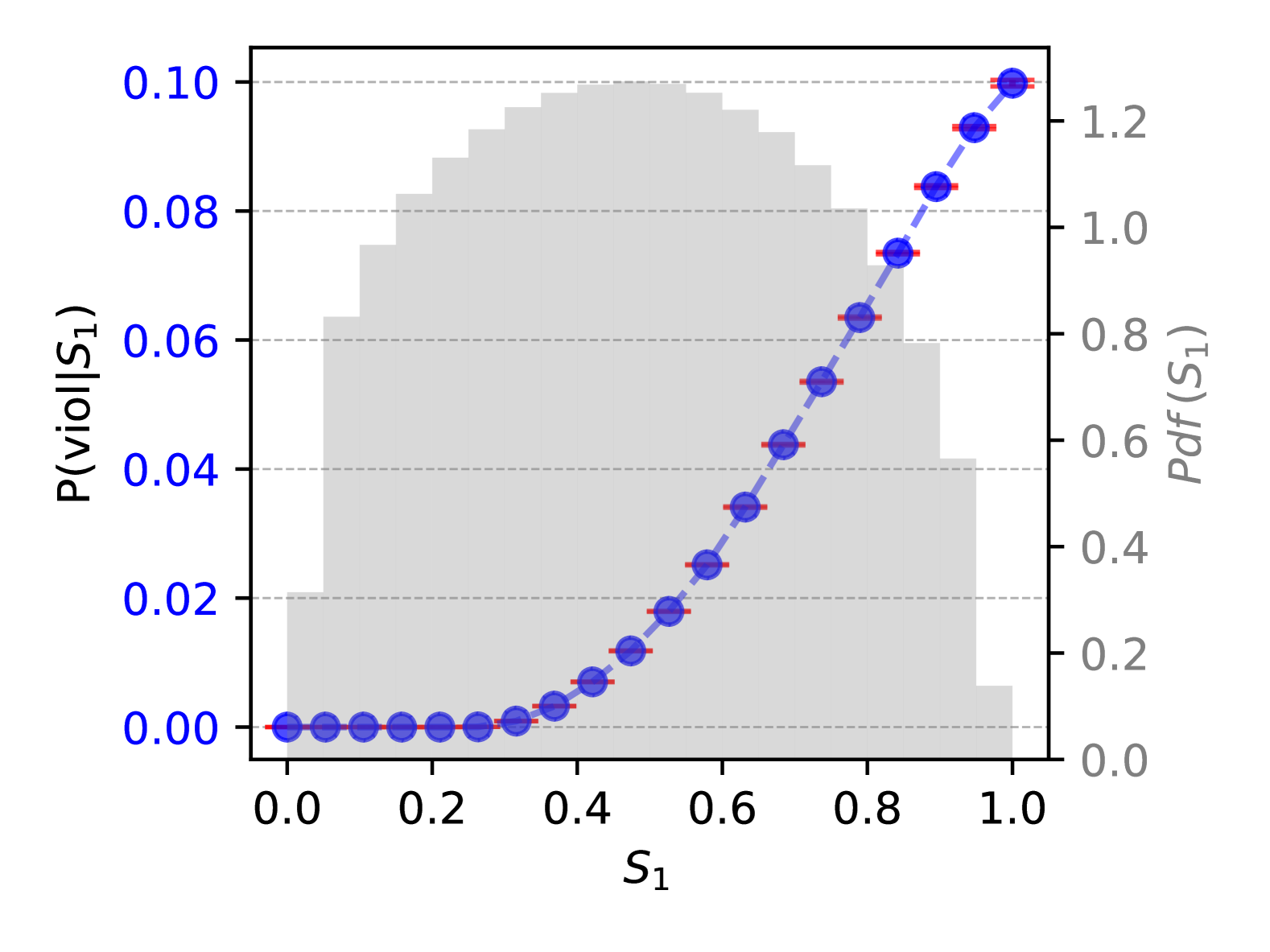
(a) Probability of violating the CHSH inequality vs the entanglement entropy $S_{1}(\rho_{A})$.

(b) Probability of violating the CHSH inequality vs the non-local non-stabilizerness $M_{\rm NL}(\ket{\psi})$.

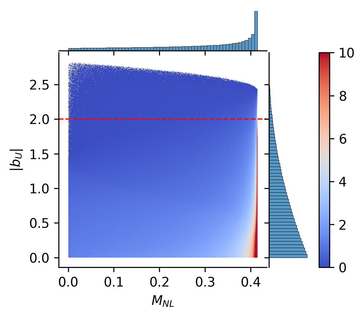
(c) Density of states in the $|b_{U}|,M_{\rm NL}$ plane. Darker regions correspond to a higher density. On the axes, the marginal probability distributions of the respective quantities.

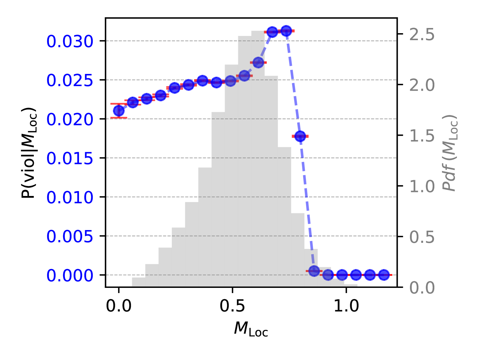
(d) Probability of violating the CHSH inequality vs the local non-stabilizerness $M_{\rm LOC}(\ket{\psi})$.

Figure 5: We sample $5\times 10^{7}$ Haar-random two-qubit states and plot in blue the probability of violating the CHSH inequality as a function of (5(a)) the entanglement entropy $S_{1}$, (5(b)) non-local non-stabilizerness $M_{NL}$, and (5(d)) local non-stabilizerness. Red error bars indicate the standard error in each bin, while the marginal probability distribution of the respective resources is shown in grey. In (5(c)), we plot the joint distribution of $|b_{U}|$ and $M_{NL}$. Here, the maximum of $|b_{U}|$ is seen to be monotonously decreasing in $M_{NL}$ and the density of states justifies the results of Fig. 5(b), see discussion in main text.

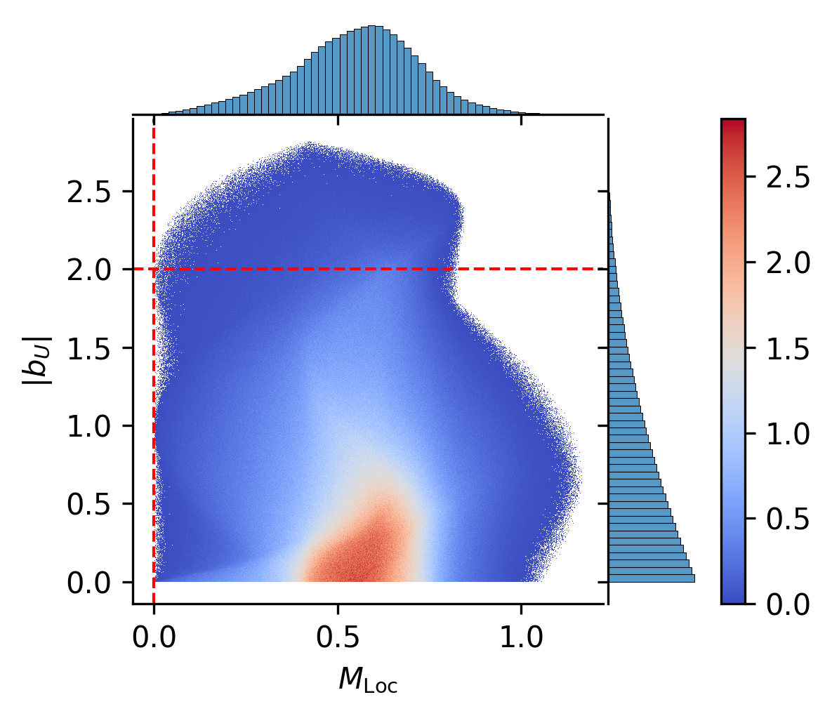
(a) Density of states in the $|b_{U}|,M_{\mathrm{LOC}}$ plane. Darker regions correspond to a higher density. On the axes, the marginal probability distributions of the respective quantities.

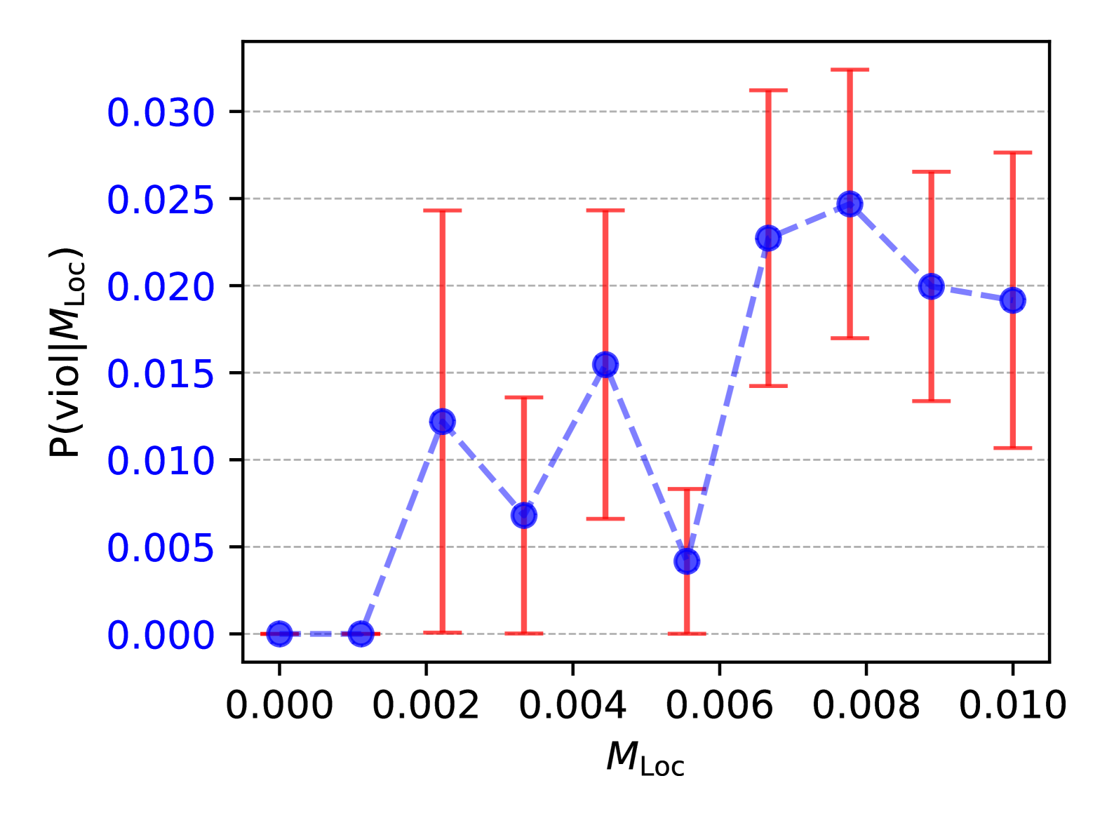
(b) Fine-grained binning near the origin for the conditional probability of violation given $M_{\mathrm{LOC}}$.

Figure 6: To understand the behavior of $P(\mathrm{viol}|M_{\mathrm{LOC}})$ for small $\mathrm{L}$, in Fig. 6(a) we plot the density of states in the $|b_{U}|,M_{\rm NL}$ plane, and in Fig. 6(b) the probability of violations for states with small values of $M_{\rm LOC}$. One can observe how states with high values of $M_{\rm LOC}$ do not violate the CHSH inequality, because of the contemporary presence of non-local non-stabilizerness. In Fig. 6(b) one can see that the probability of violations tends to zero when $M_{\rm LOC}\to 0$.

To obtain a more detailed understanding, we analyze numerically the probability of violating the CHSH inequality given a fixed amount of resources contained in the state, let them be entanglement or non-stabilizerness. In practice, we compute numerically the conditional probabilities

$$P_{B|Y}(b,y)=\frac{\langle\delta(b_{U}-b)\delta(Y_{U}-y)\rangle_{\mathcal{U}}}{P_{Y}(y)}\,,$$ (42)

where $Y$ is a given resource, and $P_{Y}(y)$ its density. The probability of violation given fixed resources $Y=y$ is then

$$\mathrm{Prob}(\mathrm{violation}|Y=y)=\int_{|b|>2}db\,P_{B|Y}(b,y)\,.$$ (43)

We perform our analysis for $Y$ equal to the entanglement entropy $E_{\mathrm{VN}}$, the non-local magic $M_{\rm NL}$, and the local non-stabilizerness $M_{\rm LOC}$. The results are shown in Fig. 5. Fig. 5(a) expresses the known fact that one needs a finite amount of entanglement to violate CHSH inequality.

In Fig. 5(b) we show the conditional probability of violating the CHSH inequality at given values of the non-local non-stabilizerness. At first glance, the plot seems to contradict Theorem 3, since the probability of violation increases with $M_{\rm NL}$. This can be explained by the fact that local and non-local magic of Haar-random states are not independent: states with high amounts of non-local magic will also possess local magic, and so the probability of violation increases. However, because of the presence of non-local magic, the violation are small, i.e. $|b_{U}|$ is slightly above 2 and way below the Tsirelson bound. This interpretation is strengthened by the plot in Fig. 5(c) where we show the density of states in the $|b_{U}|,M_{\rm NL}$ plane: for small values of $M_{\rm NL}$ there a low density of states violating the CHSH inequality, but at the same time these states can reach higher values of the violation. As $M_{\rm NL}$ increases, the maximum value of $|b_{U}|$ decreases, in accordance with Eq. (22).

Finally, in Fig. 5(d) we plot the probability of violations given $M_{\mathrm{LOC}}$. One can observe that the probability is non monotone with respect to local non-stabilizerness confirming the non-trivial interplay between local and non-local magic, since states with high amounts of local non-stabilizerness are constrained to have also large amounts of non-local non-stabilizerness, hindering the possibility of non-local violations. Note that, according to Theorem 2, $P_{\mathrm{viol}}=0$ when $M_{\mathrm{LOC}}=0$. The behavior of $P(\mathrm{viol}|M_{\mathrm{LOC}})$ for small $M_{\mathrm{LOC}}$ is detailed in Fig. 6 where it is confirmed that $P_{\mathrm{viol}}\to 0$ when $M_{\mathrm{LOC}}\to 0$.

5.2 Isospectral twirling and ensembles of unitary operators

Here we provide a systematic way to obtain a useful heuristic for the CHSH violation with limited control. The strategy is the following: we compute analytically the first two moments of the distribution of $b_{U}$ given by $d\mu_{U}$. Using the Chebyshev inequality, we argue about the most promising ensembles, i.e. those that, according to the inequality, give the largest probability of violation. Then, numerically, we verify if the promising ensembles do indeed (mostly) provide a better likelihood for a violation. To this end, we will employ the technique of isospectral twirling [64, 65] that has been developed to model situations where one has good control over the eigenvalues of a unitary $U$ but limited control over its eigenstates. We use this technique to construct ensembles $\mathcal{E}$ of unitaries that provide higher probability of violating the CHSH inequalities. We will construct the ensembles by utilizing insights given by structural properties of $U$ informed by the theorems of the previous sections. We first define the ensemble $\mathcal{E}\equiv\{g^{\dagger}U_{c}g|g\in\mathcal{G}\}$ associated to a core unitary $U_{\mathrm{c}}$ and $\mathcal{G}\subseteq\mathcal{U}(d)$ being a subgroup of the full unitary group $\mathcal{U}(d)$. From now on, the unitary $U_{\mathrm{c}}$ fixing the spectrum will be called the core and the group $\mathcal{G}$ will be explicitly denoted in the average operation $\langle\cdot\rangle_{\mathcal{G}}$. Given the core operator $U_{\mathrm{c}}$, the ensemble $\mathcal{E}$ consists of operators with the same eigenvalues as $U_{\mathrm{c}}$ but with eigenvectors determined by the action of $\mathcal{G}$ on $U_{\mathrm{c}}$. One can think that isospectral twirling mimics a situation where an experimenter tries to prepare the core unitary $U_{\mathrm{c}}$ and achieves in preparing the ensemble $\mathcal{E}$ due to the effect of noise. For each given $\mathcal{G}$ we will compute the mean and the variance of the distribution of $b_{U}$ over $\mathcal{E}$, namely $\langle b_{U}\rangle_{\mathcal{G}}$ and $\mathsf{Var}_{\mathcal{G}}(b_{U})$. It turns out that, see [64]

$$\langle b_{U}\rangle_{\mathcal{G}} = {\rm Tr}\left[T_{2}(B_{0}\otimes\omega_{0})\mathcal{R}_{\mathcal{G}}^{(2)}(U^{\otimes 1,1})\right]$$ (44)

$$\mathsf{Var}_{\mathcal{G}}(b_{U}) = \langle b_{U}^{2}\rangle_{\mathcal{G}}-\langle b_{U}\rangle_{\mathcal{G}}^{2}$$ (45)

where $b_{U}^{2}={\rm Tr}\left[T_{(13)(24)}\mathcal{R}_{\mathcal{G}}^{(4)}(U^{\otimes 2,2})(\omega_{0}^{\otimes 2}\otimes B_{0}^{\otimes 2})\right]$ and the isospectral twirling of order $k$ of a unitary operator $U$ is defined as:

$$\mathcal{R}_{\mathcal{G}}^{(2k)}(U):=\int_{\mathcal{G}}\,d\mu_{G}G^{{\dagger}\otimes 2k}U^{\otimes k,k}G^{\otimes 2k}$$ (46)

where $U^{\otimes k,k}=U^{\otimes k}\otimes U^{{\dagger}\otimes k}$ and the $T_{\pi}$ are operators for the permutations of $2k$ objects $\pi$. In practice, the isospectral twirling of order $k$ of an operator $U$ is the order $2k$ moment of the operator $U$. The result of this operation is an operator whose spectrum is the same as that of $U$, where the eigenvectors have been averaged over all elements of the group $\mathcal{G}$. The details of the evaluation of $\mathcal{R}_{\mathcal{G}}^{(2k)}(U)$ for several instances of $\mathcal{G}$ and $U$ are given in A.2.

We now provide some examples. First we consider as core operators a couple of Clifford unitaries, a simple CNOT $U_{\mathrm{c}}=C_{X}$ which leaves the state $\ket{00}$ invariant and $U_{\mathrm{c}}=C_{X}(H\otimes I)$ that prepares the maximally entangled state $|\Phi^{+}\rangle$. We also consider $U_{\mathrm{c}}=W(\theta)$ that prepares the maximal violating state for $\theta=\pi/4$. For the group $\mathcal{G}$ we consider both the full unitary group $\mathcal{U}$ and the Clifford group $\mathcal{C}$ applied symmetrically on both qubits or only on qubit $A$ or qubit $B$. In view of Theorem 2, we expect that asymmetric twirling will give better results for the probability of violation. The analytic expressions for the corresponding mean and standard deviation are shown in Table 1. Note that the expressions for the mean coincide for the two groups, but differ for the standard deviation due to the fact that the Clifford group is a 3-design but not a 4-design, and so averages over $\mathcal{C}$ and $\mathcal{U}$ coincide up to the third moments [66]. In Figure 7 we plot the means and variances for $U_{\mathrm{c}}=W(\theta)$ as a function of $\theta$.

$\langle\rangle_{\mathcal{G}}$	$C_{X}$	$C_{X}(H\otimes I)$	$W(\theta)$
$\langle b_{U}\rangle_{\mathcal{U}}$	$0.2$	$1/15$	$\frac{1}{15}(2\sin(\theta)+1)$
$\mathsf{Var}_{\mathcal{U}}(b_{U})$	$0.79$	$0.80$	$\frac{-22\sin(\theta)+26\cos(2\theta)+5016}{6300}$
$\mathsf{Var}_{\mathcal{C}}(b_{U})$	$0.98$	$1.59$	$\frac{-64\sin(\theta)+1440\cos(\theta)+357\cos(2\theta)+3937}{3600}$
$\langle b_{U}\rangle_{\mathcal{U}_{A}}$	$-2/3$	1/3	$\frac{1}{3}(\sin(\theta)+1)$
$\mathsf{Var}_{\mathcal{U}_{A}}(b_{U})$	$37/45$	$31/45$	$\frac{-7\sin(\theta)+\cos(2\theta)+45}{45}$
$\mathsf{Var}_{\mathcal{C}_{A}}(b_{U})$	$8/9$	$19/18$	$\frac{-2\sin(\theta)-\cos(2\theta)+3}{36}$
$\langle b_{U}\rangle_{\mathcal{U}_{B}}$	$1$	$2/3$	$\frac{2}{3}(\sin(\theta)+\cos(\theta))$
$\mathsf{Var}_{\mathcal{U}_{B}}(b_{U})$	$0$	$37/45$	$\frac{\sin(2\theta)+37}{45}$
$\mathsf{Var}_{\mathcal{C}_{B}}(b_{U})$	$0$	$8/9$	$\frac{4\sin(\theta)\cos(\theta)+8}{9}$

Table 1: Summary of the isospectral twirling for the operators $C_{X}=\outerproduct{0}{0}\otimes{I}_{B}+\outerproduct{1}{1}\otimes X_{B}$ and $W(\theta)\equiv(R_{y}(\theta)\otimes I)C_{X}(H\otimes I)$. The leftmost column indicates the quantity that is being averaged, together with the group over which the isospectral twirling is performed. The other columns show the corresponding value of the isospectral twirling when the argument of the twirling is the unitary operator indicated at the top of the column. Notice also that the functions correponding to the rightmost column are plotted in Fig. 7.

Looking at Fig. 7 we note that the mean $\langle b_{U}\rangle_{\mathcal{G}}$ tends to be larger when obtained by twirling on only one qubit as opposed to both qubits symmetrically and the standard deviations tend to be larger, apart from a small range of $\theta$ in Fig. 7(c), when using the Clifford group instead of the full unitary group.

Based on Fig. 7 one can make an educated guess of what are the best core unitaries $U_{\mathrm{c}}$ and groups $\mathcal{G}$ to obtain an ensemble of operators leading to a higher probability of CHSH violations. One simply looks for situations where the mean $|\langle b_{U}\rangle_{\mathcal{G}}|$ is large and the fluctuations are also large, so that CHSH violations are more likely.

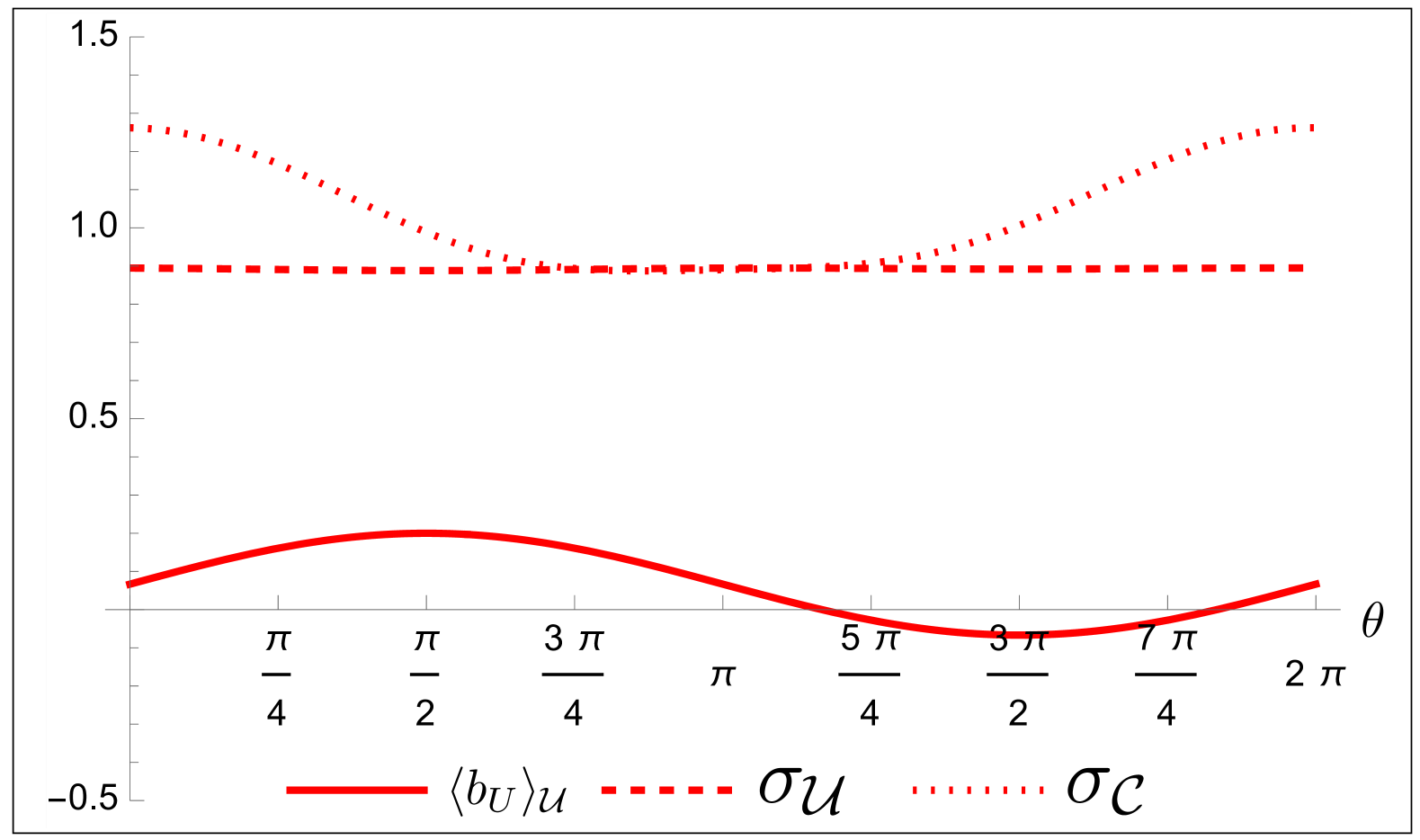
(a)

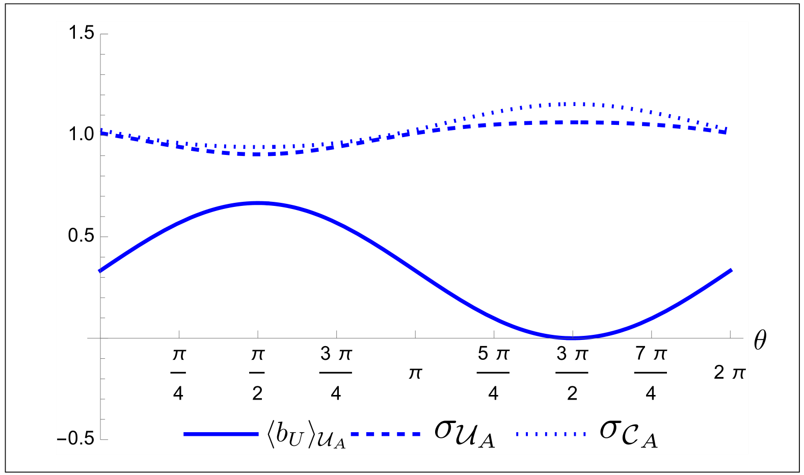
(b)

(c)

Figure 7: Plots of the average $\langle b_{U}\rangle_{\mathcal{G}}$ and of standard deviations $\sigma_{\mathcal{G}}:=\sqrt{\mathsf{Var}_{\mathcal{G}}(b_{U})}$ under isospectral twirling over the groups $\mathcal{G}=\mathcal{U},\mathcal{C}$ of the operator $U_{\rm viol}$. In every plot the solid line indicates the average, while the dashed and dotted lines indicate the average standard deviation with respect to the unitary and Clifford group respectively. Panel (a) shows the results when the average is performed over both qubit, while Panel (b) and (c) show the results when the average is performed on only one of the two qubit.

$U_{c}$	$P_{\rm viol}(\mathcal{U})$	$P_{\rm viol}(\mathcal{U}_{A})$	$P_{\rm viol}(\mathcal{U}_{B})$	$P_{\rm viol}(\mathcal{C})$	$P_{\rm viol}(\mathcal{C}_{A})$	$P_{\rm viol}(\mathcal{C}_{B})$	$\mathcal{M}_{2}(U)$
$C_{X}$	2.2%	10.8%	0	0	0	0	0
$C_{X}(H\otimes{I})$	2.5%	8.3%	10.8%	0	0	0	0
$W(\pi/2)$	2.2%	10.9%	10.8%	0	0	0	0
$W(\pi/3)$	2.3%	9.6%	17.2%	0.3%	4.2%	16.6%	0.240
$W(\pi/4)$	2.3%	8.7%	17.8%	0.3%	4.1%	16.7%	0.332
$W(\pi/8)$	2.4%	8.2%	16.1%	0.3%	4.0%	16.6%	0.154
$\tilde{C}_{X}$	2.2%	0	10.8%	0	0	0	0
$\tilde{C}_{X}({I}\otimes H)$	2.5%	10.8%	8.3%	0	0	0	0
$\tilde{W}(-\pi/2)$	2.2%	10.8%	10.9%	0	0	0	0
$\tilde{W}(-\pi/3)$	2.3%	17.2%	9.6%	0.3%	16.6%	4.2%	0.240
$\tilde{W}(-\pi/4)$	2.3%	17.8%	8.7%	0.3%	16.7%	4.1%	0.332
$\tilde{W}(-\pi/8)$	2.4%	16.1%	8.2%	0.3%	16.6%	4.0%	0.154

Table 2: Probability of violating the CHSH inequality via isospectral twirling. $P_{\rm viol}(\mathcal{G})$ is the probability of violation under isospectral twirling over the group $\mathcal{G}$. Recall the definition for the core $W(\theta)\equiv(R_{y}(\theta)\otimes{I})C_{X}(H\otimes{I})$ . The tilde operators are just the corresponding operators with the role of $A$ and $B$ exchanged.

In Table 2 we give the probabilities of violating the CHSH inequality in this setting. Together with $W(\theta=\pi/4)$ we also include results for $\theta=\pi/2,\pi/3,\pi/8$ for comparison. Based on the results of Table 2 we can draw several conclusions: i) twirling over both qubits symmetrically gives $P\mathrm{viol}$ almost equal to the full Haar result when using $\mathcal{G}=\mathcal{U}$ while it result in very small $P\mathrm{viol}$ when using $\mathcal{G}=\mathcal{C}$ (of course probabilities are exactly zero when the entire ensemble is made of Clifford unitaries because of Theorem 1); ii) despite the fact that $C_{X}$ prepares the $\ket{00}$ state, the effect of twirling over the control qubit gives fairly large $P\mathrm{viol}$ (twirling over the idler gives $P\mathrm{viol}=0$). This effect can be understood by looking at Table 1 since the values of the mean and variance are large when twirling over the control qubit; iii) the values of $P\mathrm{viol}$ for $U_{\mathrm{c}}=C_{X}(H\otimes I)$ are comparable and can also be understood by looking at Table 1; iv) of course the highest value for $P\mathrm{viol}$ is obtained using $W(\pi/4)$ as core operator having the foresight of using asymmetric twirling. However, fairly large error in the angle $\theta$ from the optimal value $\pi/4$ produce similarly good results; v) surprisingly, performing the isospectral twirling using the Clifford group on only one qubit gives a probability of violation that is comparable with the one obtained by averaging over the unitary group.

Overall, by mean of the isospectral twirling, we have shown how to build ensembles of unitary operators with large probability of non-local violations. Our finding are of course consistent with the theorems we proved, namely that in absence of non-stabilizer resources it is impossible to violate the CHSH inequality as well as the fact that resources must be asymmetric with respect to the qubits.

6 Conclusions and outlook

The interplay between non-stabilizer - measured by SE - and entanglement resources is fundamental for the violation of the CHSH inequality. As customary in quantum resource theory, we initialize the system in a state without resources and after unitary evolution we measure in bases that are also resource free. In this way, all the resources are injected in the unitary evolution.

The structure of the unitary evolution places conditions on the violation of the CHSH inequality. Specifically, in order to obtain a violation it must be both entangling and have non stabilizing power. Moreover, it must be asymmetric and - surprisingly - the non-stabilizer resource SE must be local. We compute the probability of violation given the resources. Then, employing results from representation theory, we systematically prepare ensembles of unitary evolutions that provide higher probability of violation. These techniques represent a modelization in quantum control, where one has limited control over the evolution one can implement in the system.

In perspective, we wonder how the proposed setting and techniques can be employed to study higher dimensional systems and study other fundamental probes of quantumness such as quantum discord and contextuality.

Appendix A Isospectral twirling

A.1 Fluctuations of $b_{U}$ for the Haar measure

In order to obtain an estimate of the probability of violation through the Chebyshev inequality, we need to compute also the fluctuations, as given by the variance $\mathsf{Var}_{U}(b_{U})$, of the expectation value of $B_{0}$. This is defined as:

$$\mathsf{Var}_{U}(b_{U})=\left\langle{\rm Tr}\left[B_{0}U\omega_{0}U^{\dagger}\right]^{2}\right\rangle_{U}-\left\langle{\rm Tr}\left[B_{0}U\omega_{0}U^{\dagger}\right]\right\rangle_{U}^{2}=\left\langle{\rm Tr}\left[B_{0}U\omega_{0}U^{\dagger}\right]^{2}\right\rangle_{U},$$ (47)

so that we need to compute:

$$\langle b_{U}^{2}\rangle_{U}=\left\langle{\rm Tr}\left[B_{0}U\omega_{0}U^{\dagger}\right]^{2}\right\rangle_{U}=\int_{\mathcal{U}}\,d\mu_{U}{\rm Tr}\left[B_{0}U\omega_{0}U^{\dagger}\right]^{2}$$ (48)

We can rewrite the argument of the Haar average as:

$$b_{U}^{2}={\rm Tr}\left[B_{0}U\omega_{0}U^{\dagger}\right]^{2}={\rm Tr}\left[B_{0}U\omega_{0}U^{\dagger}\otimes B_{0}U\omega_{0}U^{\dagger}\right]={\rm Tr}\left[B_{0}^{\otimes 2}(U^{\otimes 2}\omega_{0}^{\otimes 2}U^{{\dagger}\otimes 2})\right].$$ (49)

Inserting this back in the average one gets:

$$\int_{\mathcal{U}}\,d\mu_{U}{\rm Tr}\left[B_{0}U\omega_{0}U^{\dagger}\right]^{2}=\int_{\mathcal{U}}\,d\mu_{U}{\rm Tr}\left[B_{0}^{\otimes 2}(U^{\otimes 2}\omega_{0}^{\otimes 2}U^{{\dagger}\otimes 2})\right]={\rm Tr}\left[B_{0}^{\otimes 2}\int_{\mathcal{U}}\,d\mu_{U}(U^{\otimes 2}\omega_{0}^{\otimes 2}U^{{\dagger}\otimes 2})\right]$$

We can see that $\mathsf{Var}_{U}(b_{U})$ depends on the second moment of the state $\omega_{0}$. The second moment of an operator $O$ is given by:

$$\mathcal{R}_{\mathcal{G}}^{(2)}(O)=\frac{1}{d^{2}-1}\left[\left({\rm Tr}\left[O\right]-d^{-1}{\rm Tr}\left[T_{2}O\right]\right)I+\left({\rm Tr}\left[T_{2}O\right]-d^{-1}{\rm Tr}\left[O\right]\right)T_{2}\right].$$ (51)

In case $O$ is the two-fold copy of a state, i.e. $O=\omega_{0}^{\otimes 2}$, one obtains: $\int_{\mathcal{U}}\,d\mu_{U}(U^{\otimes 2}\omega_{0}^{\otimes 2}U^{{\dagger}\otimes 2})=\frac{1}{20}I+\frac{1}{20}T_{2}$. Putting this back into the trace we get $\frac{1}{20}\left({\rm Tr}\left[B_{0}^{\otimes 2}I\right]+{\rm Tr}\left[B_{0}^{\otimes 2}T_{2}\right]\right)=\frac{1}{5}{\rm Tr}\left[{I}_{4}\right]=\frac{4}{5}$ so that $\sigma_{B_{0}}=\frac{2}{\sqrt{5}}$.

Having the variance one can apply the Chebyshev inequality to obtain a first, rough, upper bound to the probability of violating the Bell inequality. The Chebyshev inequality states that the probability of a random variable $X$ to differ from its average value $\bar{X}$ is bounded as $P(\left|X-\bar{X}\right|\geq k\sigma)\leq\frac{1}{k^{2}}$. In our case the average value is $0$, while $\sigma=2/\sqrt{5}$, which means that in order for ${\rm Tr}\left[B_{0}U\omega_{0}U^{\dagger}\right]$ to be greater than $2$ one has to set $k=\sqrt{5}$, so that:

$$P(|{\rm Tr}\left[B_{0}U\omega_{0}U^{\dagger}\right]|\geq 2)\leq\frac{1}{5}.$$ (52)

A.2 Averages from representation theory

Let us now go back to the expectation value of $B_{0}$ and rewrite it as:

$${\rm Tr}\left[B_{0}U\omega_{0}U^{\dagger}\right]={\rm Tr}\left[T_{2}(B_{0}U\otimes\omega_{0}U^{\dagger})\right]={\rm Tr}\left[T_{2}(B_{0}\otimes\omega_{0})U^{\otimes 1,1}\right]$$ (53)

where we applied the swap trick ${\rm Tr}\left[AB\right]={\rm Tr}\left[T_{2}(A\otimes B)\right]$. Applying the isospectral twirling to the expression above we get:

$$\langle b_{U}\rangle_{\mathcal{G}}=\langle{\rm Tr}\left[B_{0}U\omega_{0}U^{\dagger}\right]\rangle_{\mathcal{G}}={\rm Tr}\left[T_{2}(B_{0}\otimes\omega_{0})\mathcal{R}_{\mathcal{G}}^{(2)}(U^{\otimes 1,1})\right]$$ (54)

We thus see that the average value of $B_{0}$ depends on the $k=1$ isospectral twirling, which corresponds to the second moment operator of $U^{\otimes 1,1}$. We can then apply Eq. (51) and compute the $k=2$ moment operator of $U^{\otimes 1,1}$, which is given by:

$$\mathcal{R}^{(2)}_{\mathcal{U}}(U^{\otimes 1,1})=\frac{1}{d^{2}-1}\left[\left({\rm Tr}\left[U^{\otimes 1,1}\right]-d^{-1}{\rm Tr}\left[T_{2}U^{\otimes 1,1}\right]\right)I+\left({\rm Tr}\left[T_{2}U^{\otimes 1,1}\right]-d^{-1}{\rm Tr}\left[U^{1,1}\right]\right)T_{2}\right].$$

The two traces can be easily evaluated:

$${\rm Tr}\left[U^{1,1}\right]=\left|{\rm Tr}\left[U\right]\right|^{2}=c_{2}(U)=\sum_{i,j}u_{i}u_{j}^{*}$$ (56)

$${\rm Tr}\left[T_{2}U^{\otimes 1,1}\right]={\rm Tr}\left[UU^{\dagger}\right]={\rm Tr}\left[I\right]=d$$ (57)

The function $c_{2}(U)$ is the two point spectral form factor of the unitary operator $U$, and as it can be seen, it only depends on the spectrum of $U$. Plugging these expressions back into the one for the isospectral twirling we obtain:

$$\mathcal{R}^{(2)}_{\mathcal{U}}(U^{\otimes 1,1})=\frac{c_{2}(U)-1}{15}I+\frac{16-c_{2}(U)}{60}T_{2}$$ (58)

We can plug this expression back into the expectation value, obtaining:

$$\langle b_{U}\rangle_{\mathcal{U}}={\rm Tr}\left[T_{(12)}(B_{0}\otimes\omega_{0})\mathcal{R}_{\mathcal{U}}^{2}(U^{\otimes 1,1})\right]=\frac{c_{2}(U)-1}{15}{\rm Tr}\left[T_{2}\left(B_{0}\otimes\omega_{0}\right)\right]=\frac{c_{2}(U)-1}{15}.$$ (59)

This expression only depends on the 2 point spectral form factor, and can thus be trivially upper bounded considering $|c_{2}(U)|\leq d^{2}=16$, leading to

$$\left|\langle b_{U}\rangle_{\mathcal{U}}\right|\leq 1$$ (60)

While this upper bound is still quite far from the one needed to observe violations of locality, two points must be noted. First, the upper bound is anyway better than the value obtained with the Haar averaged state. Second, this quantity only depends on the spectrum of $U$, and thus we can hope that, in presence of large enough fluctuations, one can optimize the choice of the unitary $U$ in order to obtain a larger probability of violating the CHSH inequality.

To pursue this path we need to compute the isospectral twirling of the variance, as defined in Eq. (47). In practice we need to compute

$$\langle b_{U}^{2}\rangle=\left\langle{\rm Tr}\left[B_{0}U\omega_{0}U^{\dagger}\right]^{2}\right\rangle_{\mathcal{G}} = \left\langle{\rm Tr}\left[T_{(13)(24)}U^{\otimes 2,2}(\omega_{0}^{\otimes 2}\otimes B_{0}^{\otimes 2})\right]\right\rangle_{\mathcal{U}}$$ (61)

$$= {\rm Tr}\left[T_{(13)(24)}\mathcal{R}_{\mathcal{G}}^{(4)}(U^{\otimes 2,2})(\omega_{0}^{\otimes 2}\otimes B_{0}^{\otimes 2})\right]$$

So, in order to compute the standard deviation under isospectral twirling we need to compute the moment of order $k=4$ of the unitary operator $U^{\otimes 2,2}$. At this point we must note that one is not forced to average over the whole unitary group, but in principle it is also possible to perform the isospectral twirling over the Clifford group. As the latter is known to form a 3-design [66], it is clear that we are going to observe a difference only when computing the standard deviation, which involves the fourth order average.

The fourth order average over the whole unitary group can be easily evaluated with the same techniques used for the $k=1,2$ moment operators, leading to the final result:

$${\rm Tr}\left[T_{(13)(24)}\mathcal{R}_{\mathcal{U}}^{(4)}(U^{\otimes 2,2})\left(\omega_{0}^{\otimes 2}\otimes B_{0}^{\otimes 2}\right)\right]=\frac{1344-4c_{2}(U)+\tilde{c}_{2}(U)+2\real[c_{3}(U)]+c_{4}(U)}{1680}$$ (62)

This expression once again depends only on the spectrum of $U$, but this time the expression features also the three and four points spectral form factor, defined as:

$$\tilde{c}_{2}(U)=\sum_{i,j}u_{i}^{2}u_{j}^{*2},\qquad c_{3}(U)=\sum_{i,j,k}u_{i}u_{j}u_{k}^{*2},\qquad c_{4}(U)=\sum_{i,j,k,\ell}u_{i}u_{j}u^{*}_{k}u^{*}_{\ell}$$ (63)

The variance under isospectral twirling $\mathsf{Var}_{\mathcal{U}}(b_{U})$ is then worth:

$$\mathsf{Var}_{\mathcal{U}}(b_{U})=\frac{4\left(41-28c_{2}\right)c_{2}+15\tilde{c}_{2}+30\real\left(c_{3}\right)+15c_{4}+20048}{25200}$$ (64)

Let us now turn to the Clifford average. The formula to perform this average has been already derived [67], and it reads:

$$\mathcal{R}_{\mathcal{C}}^{(4)}(U)=\int_{\mathcal{C}}d\mu_{C}C^{{\dagger}\otimes 4}U^{\otimes 2,2}C^{\otimes 4}=\sum_{\pi,\sigma\in S_{4}}W^{+}_{\pi\sigma}{\rm Tr}\left[T_{\pi}QU^{\otimes 2,2}\right]QT_{\sigma}+W^{-}_{\pi\sigma}{\rm Tr}\left[T_{\pi}Q^{\perp}U^{\otimes 2,2}\right]Q^{\perp}T_{\sigma}$$

(65)

where $Q^{\perp}=I^{\otimes 4}-Q$, and the Weingarten coefficients $W^{\pm}$ can be computed in terms of the characters of the symmetric group representations as:

$$W^{\pm}_{\pi\sigma}=\sum_{\lambda}\frac{d_{\lambda}^{2}}{(4!)^{2}}\frac{\chi^{\lambda}(\pi\sigma)}{D^{\pm}_{\lambda}}$$ (66)

where $\lambda$ labels the irreducible representations of the symmetric group $S_{4}$, $d_{\lambda}$ is the dimension of the corresponding irrep, $\chi_{\lambda}(\pi\sigma)$ is the character of the corresponding permutation and $D^{+}_{\lambda}={\rm Tr}\left[P_{\lambda}Q\right]$, $D^{-}_{\lambda}={\rm Tr}\left[P_{\lambda}Q^{\perp}\right]$, $P_{\lambda}$ being the projector onto the irrep $\lambda$.

One can then use Eq. (65) to compute the variance under isospectral twirling over the Clifford group to obtain:

$$\mathsf{Var}_{\mathcal{C}}(b_{U})=\frac{7}{9}+\frac{|c_{U^{2}}|^{2}+2\real[c_{U}^{*2}c_{U^{2}}]+|c_{U}|^{4}}{80}-\frac{|c_{UU^{\dagger}}|^{2}+c_{(UU^{\dagger})^{2}}}{72}-\left(\frac{c_{2}(U)-1}{15}\right)^{2}$$ (67)

where we have defined:

$$|c_{U}|^{4}= d^{-2}\sum_{P}|{\rm Tr}\left[PU\right]|^{4}=d^{-2}\sum_{P}\sum_{i}|e^{-i\phi_{i}}\bra{\phi_{i}}U\ket{\phi_{i}}|^{4},$$ (68)

$$|c_{U^{2}}|^{2} = d^{-2}\sum_{P}|{\rm Tr}\left[PUPU\right]|^{2}=d^{-2}\sum_{P}\sum_{i,j}|e^{-i(\phi_{i}+\phi_{j})}\bra{\phi_{j}}U\outerproduct{\phi_{i}}{\phi_{i}}U\ket{\phi_{j}}|^{2},$$ (69)

$$c_{U}^{*2}c_{U^{2}} = d^{-2}\sum_{P}{\rm Tr}\left[PU^{\dagger}\right]^{2}{\rm Tr}\left[PUPU\right]$$ (70)

$$= d^{-2}\sum_{P}\sum_{i,j,k}e^{-i(\phi_{i}+\phi_{j}-2\phi_{k})}\bra{\phi_{j}}U\outerproduct{\phi_{i}}{\phi_{i}}U\ket{\phi_{j}}\bra{\phi_{k}}U^{\dagger}\ket{\phi_{k}}^{2},$$

$$|c_{UU^{\dagger}}|^{2} = d^{-2}\sum_{P}|{\rm Tr}\left[PUPU^{\dagger}\right]|^{2}=d^{-2}\sum_{P}\sum_{i,j}|e^{-i(\phi_{i}-\phi_{j})}\bra{\phi_{j}}U\outerproduct{\phi_{i}}{\phi_{i}}U^{\dagger}\ket{\phi_{j}}|^{2},$$ (71)

$$c_{(UU^{\dagger})^{2}} = d^{-2}\sum_{P}{\rm Tr}\left[UPU^{\dagger}PUPU^{\dagger}\right]$$ (72)

$$= d^{-2}\sum_{P}\sum_{i,j,k,\ell}e^{-i(\phi_{i}+\phi_{j}-\phi_{k}-\phi_{\ell})}\bra{\phi_{i}}U\outerproduct{\phi_{j}}{\phi_{j}}U^{\dagger}\outerproduct{\phi_{k}}{\phi_{k}}U\outerproduct{\phi_{\ell}}{\phi_{\ell}}U^{\dagger}\ket{\phi_{i}}.$$

where we have written the unitary operator $U$ as $\sum_{i}e^{-i\phi_{i}}\outerproduct{\phi_{i}}{\phi_{i}}$ where $\ket{\phi_{i}}$ are eigenvectors of $U$ and $e^{-i\phi_{i}}$ the corresponding eigenvalues. Notice that in contrast with the average over the unitary group, in this case it is not possible to give a closed form of the standard deviation in terms of the spectrum of $U$ alone. Indeed, the isospectral twirling over the Clifford group does depend on the matrix elements of $U$ in the Pauli basis. This means that in order to evaluate the standard deviation in this case we need the full expression of the unitary operator $U$.

References

- Clauser et al. [1969] John F. Clauser, Michael A. Horne, Abner Shimony, and Richard A. Holt. Proposed experiment to test local hidden-variable theories. Phys. Rev. Lett., 23:880–884, Oct 1969. doi: 10.1103/PhysRevLett.23.880. URL https://link.aps.org/doi/10.1103/PhysRevLett.23.880.
- Howard [2015] Mark Howard. Maximum nonlocality and minimum uncertainty using magic states. Phys. Rev. A, 91:042103, Apr 2015. doi: 10.1103/PhysRevA.91.042103. URL https://link.aps.org/doi/10.1103/PhysRevA.91.042103.
- Howard et al. [2014] Mark Howard, Joel Wallman, Victor Veitch, and Joseph Emerson. Contextuality supplies the ‘magic’ for quantum computation. Nature, 510(7505):351–355, 2014. ISSN 1476-4687. doi: 10.1038/nature13460. URL https://doi.org/10.1038/nature13460.
- Howard and Vala [2012] Mark Howard and Jiri Vala. Nonlocality as a benchmark for universal quantum computation in ising anyon topological quantum computers. Phys. Rev. A, 85:022304, Feb 2012. doi: 10.1103/PhysRevA.85.022304. URL https://link.aps.org/doi/10.1103/PhysRevA.85.022304.
- Macedo et al. [2025] Rafael A. Macedo, Patrick Andriolo, Santiago Zamora, Davide Poderini, and Rafael Chaves. Witnessing magic with bell inequalities, 2025. URL https://arxiv.org/abs/2503.18734.
- Gottesman [1997] Daniel Gottesman. Stabilizer Codes and Quantum Error Correction. PhD thesis, Caltech, Pasadena, May 1997. URL http://arxiv.org/abs/quant-ph/9705052. arXiv:quant-ph/9705052.
- Gottesman [1998] Daniel Gottesman. The Heisenberg Representation of Quantum Computers, July 1998. URL http://arxiv.org/abs/quant-ph/9807006. arXiv:quant-ph/9807006.
- Aaronson and Gottesman [2004] Scott Aaronson and Daniel Gottesman. Improved simulation of stabilizer circuits. Phys. Rev. A, 70(5):052328, November 2004. doi: 10.1103/PhysRevA.70.052328. URL https://link.aps.org/doi/10.1103/PhysRevA.70.052328. Publisher: American Physical Society.
- Zhou et al. [2020] Shiyu Zhou, Zhi-Cheng Yang, Alioscia Hamma, and Claudio Chamon. Single T gate in a Clifford circuit drives transition to universal entanglement spectrum statistics. SciPost Phys., 9:087, 2020. doi: 10.21468/SciPostPhys.9.6.087. URL https://scipost.org/10.21468/SciPostPhys.9.6.087.
- Leone et al. [2021a] Lorenzo Leone, Salvatore F. E. Oliviero, You Zhou, and Alioscia Hamma. Quantum Chaos is Quantum. Quantum, 5:453, May 2021a. ISSN 2521-327X. doi: 10.22331/q-2021-05-04-453. URL https://doi.org/10.22331/q-2021-05-04-453.
- Leone et al. [2022a] Lorenzo Leone, Salvatore F. E. Oliviero, and Alioscia Hamma. Stabilizer R\’enyi Entropy. Phys. Rev. Lett., 128(5):050402, February 2022a. doi: 10.1103/PhysRevLett.128.050402. URL https://link.aps.org/doi/10.1103/PhysRevLett.128.050402. Publisher: American Physical Society.
- Leone and Bittel [2024] Lorenzo Leone and Lennart Bittel. Stabilizer entropies are monotones for magic-state resource theory, April 2024. URL http://arxiv.org/abs/2404.11652. arXiv:2404.11652 [quant-ph].
- Oliviero et al. [2022a] Salvatore F E Oliviero, Lorenzo Leone, Alioscia Hamma, and Seth Lloyd. Measuring magic on a quantum processor. npj Quantum Information, 8(1):148, 2022a. ISSN 2056-6387. doi: 10.1038/s41534-022-00666-5. URL https://doi.org/10.1038/s41534-022-00666-5.
- Lami and Collura [2023] Guglielmo Lami and Mario Collura. Nonstabilizerness via perfect pauli sampling of matrix product states. Phys. Rev. Lett., 131:180401, Oct 2023. doi: 10.1103/PhysRevLett.131.180401. URL https://link.aps.org/doi/10.1103/PhysRevLett.131.180401.
- Tarabunga et al. [2024] Poetri Sonya Tarabunga, Emanuele Tirrito, Mari Carmen Bañuls, and Marcello Dalmonte. Nonstabilizerness via matrix product states in the pauli basis. Phys. Rev. Lett., 133:010601, Jul 2024. doi: 10.1103/PhysRevLett.133.010601. URL https://link.aps.org/doi/10.1103/PhysRevLett.133.010601.
- Tarabunga et al. [2023a] Poetri Sonya Tarabunga, Emanuele Tirrito, Titas Chanda, and Marcello Dalmonte. Many-body magic via pauli-markov chains—from criticality to gauge theories. PRX Quantum, 4:040317, Oct 2023a. doi: 10.1103/PRXQuantum.4.040317. URL https://link.aps.org/doi/10.1103/PRXQuantum.4.040317.
- Oliviero et al. [2021a] Salvatore F E Oliviero, Lorenzo Leone, and Alioscia Hamma. Transitions in entanglement complexity in random quantum circuits by measurements. Physics Letters A, 418:127721, 2021a. ISSN 0375-9601. doi: https://doi.org/10.1016/j.physleta.2021.127721. URL https://www.sciencedirect.com/science/article/pii/S0375960121005855.
- Oliviero et al. [2022b] Salvatore F. E. Oliviero, Lorenzo Leone, You Zhou, and Alioscia Hamma. Stability of topological purity under random local unitaries. SciPost Phys., 12:096, 2022b. doi: 10.21468/SciPostPhys.12.3.096. URL https://scipost.org/10.21468/SciPostPhys.12.3.096.
- True and Hamma [2022] Sarah True and Alioscia Hamma. Transitions in Entanglement Complexity in Random Circuits. Quantum, 6:818, September 2022. ISSN 2521-327X. doi: 10.22331/q-2022-09-22-818. URL https://doi.org/10.22331/q-2022-09-22-818.
- Catalano et al. [2024] A. G. Catalano, J. Odavić, G. Torre, A. Hamma, F. Franchini, and S. M. Giampaolo. Magic phase transition and non-local complexity in generalized state, 2024. URL https://arxiv.org/abs/2406.19457.
- Li et al. [2024] Gongchu Li, Lei Chen, Si-Qi Zhang, Xu-Song Hong, Huaqing Xu, Yuancheng Liu, You Zhou, Geng Chen, Chuan-Feng Li, Alioscia Hamma, and Guang-Can Guo. Measurement induced magic resources, 2024. URL https://arxiv.org/abs/2408.01980.
- Odavić et al. [2025] Jovan Odavić, Michele Viscardi, and Alioscia Hamma. Stabilizer entropy in non-integrable quantum evolutions, 2025. URL https://arxiv.org/abs/2412.10228.
- Jasser et al. [2025] Barbara Jasser, Jovan Odavic, and Alioscia Hamma. Stabilizer entropy and entanglement complexity in the sachdev-ye-kitaev model, 2025. URL https://arxiv.org/abs/2502.03093.
- Cao et al. [2024] ChunJun Cao, Gong Cheng, Alioscia Hamma, Lorenzo Leone, William Munizzi, and Savatore F. E. Oliviero. Gravitational back-reaction is magical, May 2024. URL http://arxiv.org/abs/2403.07056. arXiv:2403.07056 [gr-qc, physics:hep-th, physics:quant-ph].
- Brökemeier et al. [2024] Florian Brökemeier, S. Momme Hengstenberg, James W. T. Keeble, Caroline E. P. Robin, Federico Rocco, and Martin J. Savage. Quantum magic and multi-partite entanglement in the structure of nuclei, September 2024. URL http://arxiv.org/abs/2409.12064.
- Chernyshev et al. [2024] Ivan Chernyshev, Caroline E. P. Robin, and Martin J. Savage. Quantum magic and computational complexity in the neutrino sector, November 2024. URL http://arxiv.org/abs/2411.04203.
- White and White [2024] Chris D. White and Martin J. White. Magic states of top quarks. Physical Review D, 110(11):116016, December 2024. doi: 10.1103/PhysRevD.110.116016. URL https://link.aps.org/doi/10.1103/PhysRevD.110.116016.
- Leone et al. [2022b] Lorenzo Leone, Salvatore F. E. Oliviero, Stefano Piemontese, Sarah True, and Alioscia Hamma. Retrieving information from a black hole using quantum machine learning. Phys. Rev. A, 106:062434, Dec 2022b. doi: 10.1103/PhysRevA.106.062434. URL https://link.aps.org/doi/10.1103/PhysRevA.106.062434.
- Leone et al. [2023] Lorenzo Leone, Salvatore F. E. Oliviero, and Alioscia Hamma. Nonstabilizerness determining the hardness of direct fidelity estimation. Phys. Rev. A, 107:022429, Feb 2023. doi: 10.1103/PhysRevA.107.022429. URL https://link.aps.org/doi/10.1103/PhysRevA.107.022429.
- Oliviero et al. [2024] Salvatore F. E. Oliviero, Lorenzo Leone, Seth Lloyd, and Alioscia Hamma. Unscrambling quantum information with clifford decoders. Phys. Rev. Lett., 132:080402, Feb 2024. doi: 10.1103/PhysRevLett.132.080402. URL https://link.aps.org/doi/10.1103/PhysRevLett.132.080402.
- Leone et al. [2024a] Lorenzo Leone, Salvatore F. E. Oliviero, Seth Lloyd, and Alioscia Hamma. Learning efficient decoders for quasichaotic quantum scramblers. Phys. Rev. A, 109:022429, Feb 2024a. doi: 10.1103/PhysRevA.109.022429. URL https://link.aps.org/doi/10.1103/PhysRevA.109.022429.
- Leone et al. [2024b] Lorenzo Leone, Salvatore F. E. Oliviero, and Alioscia Hamma. Learning t-doped stabilizer states. Quantum, 8:1361, May 2024b. ISSN 2521-327X. doi: 10.22331/q-2024-05-27-1361. URL https://doi.org/10.22331/q-2024-05-27-1361.
- Hou et al. [2025] Zong-Yue Hou, ChunJun Cao, and Zhi-Cheng Yang. Stabilizer entanglement as a magic highway, 2025. URL https://arxiv.org/abs/2503.20873.
- Gu et al. [2024] Andi Gu, Salvatore F. E. Oliviero, and Lorenzo Leone. Magic-induced computational separation in entanglement theory, 2024. URL https://arxiv.org/abs/2403.19610.
- Wang and Li [2023] Yiran Wang and Yongming Li. Stabilizer Rényi entropy on qudits. Quantum Information Processing, 22(12):444, 2023. ISSN 1573-1332. doi: 10.1007/s11128-023-04186-9. URL https://doi.org/10.1007/s11128-023-04186-9.
- Yang et al. [2017] Zhi-Cheng Yang, Alioscia Hamma, Salvatore M. Giampaolo, Eduardo R. Mucciolo, and Claudio Chamon. Entanglement complexity in quantum many-body dynamics, thermalization, and localization. Phys. Rev. B, 96:020408, Jul 2017. doi: 10.1103/PhysRevB.96.020408. URL https://link.aps.org/doi/10.1103/PhysRevB.96.020408.
- Tirrito et al. [2024] Emanuele Tirrito, Poetri Sonya Tarabunga, Gugliemo Lami, Titas Chanda, Lorenzo Leone, Salvatore F. E. Oliviero, Marcello Dalmonte, Mario Collura, and Alioscia Hamma. Quantifying nonstabilizerness through entanglement spectrum flatness. Phys. Rev. A, 109:L040401, Apr 2024. doi: 10.1103/PhysRevA.109.L040401. URL https://link.aps.org/doi/10.1103/PhysRevA.109.L040401.
- Iannotti et al. [2025] Daniele Iannotti, Gianluca Esposito, Lorenzo Campos Venuti, and Alioscia Hamma. Entanglement and stabilizer entropies of random bipartite pure quantum states, 2025. URL https://arxiv.org/abs/2501.19261.
- Oliviero et al. [2022c] Salvatore F. E. Oliviero, Lorenzo Leone, and Alioscia Hamma. Magic-state resource theory for the ground state of the transverse-field ising model. Phys. Rev. A, 106:042426, Oct 2022c. doi: 10.1103/PhysRevA.106.042426. URL https://link.aps.org/doi/10.1103/PhysRevA.106.042426.
- Odavić et al. [2023] Jovan Odavić, Tobias Haug, Gianpaolo Torre, Alioscia Hamma, Fabio Franchini, and Salvatore Marco Giampaolo. Complexity of frustration: A new source of non-local non-stabilizerness. SciPost Phys., 15:131, 2023. doi: 10.21468/SciPostPhys.15.4.131. URL https://scipost.org/10.21468/SciPostPhys.15.4.131.
- Rattacaso et al. [2023] Davide Rattacaso, Lorenzo Leone, Salvatore F. E. Oliviero, and Alioscia Hamma. Stabilizer entropy dynamics after a quantum quench. Phys. Rev. A, 108:042407, Oct 2023. doi: 10.1103/PhysRevA.108.042407. URL https://link.aps.org/doi/10.1103/PhysRevA.108.042407.
- Tarabunga et al. [2023b] Poetri Sonya Tarabunga, Emanuele Tirrito, Titas Chanda, and Marcello Dalmonte. Many-body magic via pauli-markov chains—from criticality to gauge theories. PRX Quantum, 4:040317, Oct 2023b. doi: 10.1103/PRXQuantum.4.040317. URL https://link.aps.org/doi/10.1103/PRXQuantum.4.040317.
- Liu and Winter [2022] Zi-Wen Liu and Andreas Winter. Many-body quantum magic. PRX Quantum, 3:020333, May 2022. doi: 10.1103/PRXQuantum.3.020333. URL https://link.aps.org/doi/10.1103/PRXQuantum.3.020333.
- Wei and Liu [2025] Fuchuan Wei and Zi-Wen Liu. Long-range nonstabilizerness from topology and correlation, 2025. URL https://arxiv.org/abs/2503.04566.
- Cepollaro et al. [2024] Simone Cepollaro, Goffredo Chirco, Gianluca Cuffaro, Gianluca Esposito, and Alioscia Hamma. Stabilizer entropy of quantum tetrahedra. Phys. Rev. D, 109:126008, Jun 2024. doi: 10.1103/PhysRevD.109.126008. URL https://link.aps.org/doi/10.1103/PhysRevD.109.126008.
- Cepollaro et al. [2025] S. Cepollaro, S. Cusumano, A. Hamma, G. Lo Giudice, and J. Odavic. Harvesting stabilizer entropy and non-locality from a quantum field, 2025. URL https://arxiv.org/abs/2412.11918.
- Falcão et al. [2025] Pedro R. Nicácio Falcão, Piotr Sierant, Jakub Zakrzewski, and Emanuele Tirrito. Magic dynamics in many-body localized systems, 2025. URL https://arxiv.org/abs/2503.07468.
- Turkeshi et al. [2025] Xhek Turkeshi, Anatoly Dymarsky, and Piotr Sierant. Pauli spectrum and nonstabilizerness of typical quantum many-body states. Phys. Rev. B, 111:054301, Feb 2025. doi: 10.1103/PhysRevB.111.054301. URL https://link.aps.org/doi/10.1103/PhysRevB.111.054301.
- Ding et al. [2025] Yi-Ming Ding, Zhe Wang, and Zheng Yan. Evaluating many-body stabilizer rényi entropy by sampling reduced pauli strings: singularities, volume law, and nonlocal magic, 2025. URL https://arxiv.org/abs/2501.12146.
- Hoshino et al. [2025] Masahiro Hoshino, Masaki Oshikawa, and Yuto Ashida. Stabilizer rényi entropy and conformal field theory, 2025. URL https://arxiv.org/abs/2503.13599.
- Horodecki et al. [1995] R Horodecki, P Horodecki, and M Horodecki. Violating Bell inequality by mixed spin-12 states: necessary and sufficient condition. Physics Letters A, 200(5):340–344, 1995. ISSN 0375-9601. doi: https://doi.org/10.1016/0375-9601(95)00214-N. URL https://www.sciencedirect.com/science/article/pii/037596019500214N.
- Qian and Wang [2025] Dongheng Qian and Jing Wang. Quantum non-local magic, 2025. URL https://arxiv.org/abs/2502.06393.
- Cirel’son [1980] B. S. Cirel’son. Quantum generalizations of Bell’s inequality. Lett Math Phys, 4(2):93–100, March 1980. ISSN 1573-0530. doi: 10.1007/BF00417500. URL https://doi.org/10.1007/BF00417500.
- Boes et al. [2022] Paul Boes, Nelly H.Y. Ng, and Henrik Wilming. Variance of relative surprisal as single-shot quantifier. PRX Quantum, 3:010325, Feb 2022. doi: 10.1103/PRXQuantum.3.010325. URL https://link.aps.org/doi/10.1103/PRXQuantum.3.010325.
- Dupuis and Fawzi [2019] Frédéric Dupuis and Omar Fawzi. Entropy accumulation with improved second-order term. IEEE Transactions on Information Theory, 65(11):7596–7612, 2019. doi: 10.1109/TIT.2019.2929564.
- Reeb and Wolf [2015] David Reeb and Michael M. Wolf. Tight bound on relative entropy by entropy difference. IEEE Transactions on Information Theory, 61(3):1458–1473, 2015. doi: 10.1109/TIT.2014.2387822.
- Yao and Qi [2010] Hong Yao and Xiao-Liang Qi. Entanglement entropy and entanglement spectrum of the kitaev model. Phys. Rev. Lett., 105:080501, Aug 2010. doi: 10.1103/PhysRevLett.105.080501. URL https://link.aps.org/doi/10.1103/PhysRevLett.105.080501.
- Schliemann [2011] John Schliemann. Entanglement spectrum and entanglement thermodynamics of quantum hall bilayers at . Phys. Rev. B, 83:115322, Mar 2011. doi: 10.1103/PhysRevB.83.115322. URL https://link.aps.org/doi/10.1103/PhysRevB.83.115322.
- Dong [2016] Xi Dong. The gravity dual of Rényi entropy. Nature Communications, 7(1):12472, 2016. ISSN 2041-1723. doi: 10.1038/ncomms12472. URL https://doi.org/10.1038/ncomms12472.
- Dong [2019] Xi Dong. Holographic rényi entropy at high energy density. Phys. Rev. Lett., 122:041602, Feb 2019. doi: 10.1103/PhysRevLett.122.041602. URL https://link.aps.org/doi/10.1103/PhysRevLett.122.041602.
- Tilma et al. [2002] Todd Tilma, Mark Byrd, and E C G Sudarshan. A parametrization of bipartite systems based on su(4) euler angles. Journal of Physics A: Mathematical and General, 35(48):10445, nov 2002. doi: 10.1088/0305-4470/35/48/315. URL https://dx.doi.org/10.1088/0305-4470/35/48/315.
- Mele [2024] Antonio Anna Mele. Introduction to Haar Measure Tools in Quantum Information: A Beginner’s Tutorial. Quantum, 8:1340, May 2024. ISSN 2521-327X. doi: 10.22331/q-2024-05-08-1340. URL https://doi.org/10.22331/q-2024-05-08-1340.
- Campos Venuti and Zanardi [2013] L. Campos Venuti and P. Zanardi. Probability density of quantum expectation values. Physics Letters A, 377(31–33):1854–1861, October 2013. ISSN 0375-9601. doi: 10.1016/j.physleta.2013.05.041. URL http://www.sciencedirect.com/science/article/pii/S037596011300529X.
- Oliviero et al. [2021b] Salvatore F. E. Oliviero, Lorenzo Leone, Francesco Caravelli, and Alioscia Hamma. Random matrix theory of the isospectral twirling. SciPost Phys., 10:076, 2021b. doi: 10.21468/SciPostPhys.10.3.076. URL https://scipost.org/10.21468/SciPostPhys.10.3.076.
- Leone et al. [2021b] Lorenzo Leone, Salvatore F. E. Oliviero, and Alioscia Hamma. Isospectral Twirling and Quantum Chaos. Entropy, 23(8):1073, August 2021b. ISSN 1099-4300. doi: 10.3390/e23081073. URL https://www.mdpi.com/1099-4300/23/8/1073. Number: 8 Publisher: Multidisciplinary Digital Publishing Institute.
- Zhu et al. [2016] Huangjun Zhu, Richard Kueng, Markus Grassl, and David Gross. The Clifford group fails gracefully to be a unitary 4-design, September 2016. URL http://arxiv.org/abs/1609.08172. arXiv:1609.08172 [quant-ph].
- Roth et al. [2018] I. Roth, R. Kueng, S. Kimmel, Y.-K. Liu, D. Gross, J. Eisert, and M. Kliesch. Recovering quantum gates from few average gate fidelities. Phys. Rev. Lett., 121:170502, Oct 2018. doi: 10.1103/PhysRevLett.121.170502. URL https://link.aps.org/doi/10.1103/PhysRevLett.121.170502.