Error estimates of an exponential wave integrator for the nonlinear Schrödinger equation with singular potential

Abstract

We analyze a first-order exponential wave integrator (EWI) for the nonlinear Schrödinger equation (NLSE) with a singular potential locally in $L^{2}$, which might be locally unbounded. The typical example is the inverse power potential such as the Coulomb potential, which is the most fundamental potential in quantum physics and chemistry. We prove that, under the assumption of $L^{2}$-potential and $H^{2}$-initial data, the $L^{2}$-norm convergence of the EWI is, roughly, first-order in one dimension (1D) and two dimensions (2D), and $\frac{3}{4}$-order in three dimensions (3D). In addition, under a stronger integrability assumption of $L^{p}$-potential for some $p>2$ in 3D, the $L^{2}$-norm convergence increases to almost ${\frac{3}{4}}+3(\frac{1}{2}-\frac{1}{p})$ order if $p\leq\frac{12}{5}$ and becomes first-order if $p>\frac{12}{5}$. In particular, our results show, to the best of our knowledge for the first time, that first-order $L^{2}$-norm convergence can be achieved when solving the NLSE with the Coulomb potential in 3D. The key advancements are the use of discrete (in time) Strichartz estimates, which allow us to handle the loss of integrability due to the singular potential that does not belong to $L^{\infty}$, and the more favorable local truncation error of the EWI, which requires no (spatial) smoothness of the potential. Extensive numerical results in 1D, 2D, and 3D are reported to confirm our error estimates and to show the sharpness of our assumptions on the regularity of the singular potentials.

65M15, 35Q55, 81Q05

1 Introduction

We consider the following Cauchy problem of the nonlinear Schrödinger equation (NLSE) of the form

(1) $$\left\{\begin{aligned} &i\partial_{t}\psi(\bm{x},t)=-\Delta\psi(\bm{x},t)+V(\bm{x})\psi(\bm{x},t)+\beta|\psi(\bm{x},t)|^{2\sigma}\psi(\bm{x},t),\quad\bm{x}\in\mathbb{R}^{d},\\ &\psi(\bm{x},0)=\psi_{0}(\bm{x}),\quad\bm{x}\in\mathbb{R}^{d},\end{aligned}\right.$$

where $t\geq 0$ is time, $\bm{x}=(x_{1},\cdots,x_{d})^{T}$ is the space variable, $d\in\{1,2,3\}$ represents the spatial dimension, $\psi=\psi(\bm{x},t)\in\mathbb{C}$ is the wave function, and $\beta\in\mathbb{R}$, $\sigma\in\mathbb{R}^{+}$ are given parameters characterizing the nonlinearity. Here, $V:=V(\bm{x})$ is a real-valued external potential and we assume that [18]

(2) $$V\in L^{2}(\mathbb{R}^{d})+L^{\infty}(\mathbb{R}^{d}):=\{au+bv\,|\,u\in L^{2}(\mathbb{R}^{d}),\ v\in L^{\infty}(\mathbb{R}^{d}),\ a,b\in\mathbb{R}\},$$

to allow for possible singularities.

The NLSE Eq. 1 has diverse applications in quantum mechanics, quantum physics and chemistry, laser beam propagation, plasma and particle physics, deep water waves, etc [45, 4, 23]. Especially, when $\sigma=1$, it is widely used in the modeling and simulation of Bose-Einstein condensates (BEC), where it is also known as the Gross-Pitaevskii equation (GPE) [39, 22]. In these applications, the potential $V$ may take different forms due to the different theoretical and experimental settings. In particular, in many cases, the potential $V$ is of low regularity and could be singular [17, 24, 33]. The most important and fundamental example is the Coulomb potential with $V(\bm{x})=-1/|\bm{x}|$, which is the quantum mechanical description of the Coulomb force between charged particles [43]. Other singular potential includes the inverse square potential with $V(\bm{x})=-1/|\bm{x}|^{2}$, the Yukawa potential (or screened Coulomb potential) with $V(\bm{x})=-e^{-|\bm{x}|}/|\bm{x}|$, the Dirac delta potential, etc [34, 46, 47]. Another important class of low-regularity or singular potential arises in the study of wave propagation in disordered media and the phenomenon of localization [2, 25, 42], where the disorder potential may belong to spaces such as $L^{\infty}$, $L^{2}$, or even the negative Sobolev spaces $H^{-\alpha}$ for some $\alpha>0$, depending on the strength and nature of the disorder.

For the (local) well-posedness of the NLSE Eq. 1 with the singular potential of $L^{p}$-type, it has been well-studied in the PDE literature, and we briefly summarize them in the following (see, e.g., the book [18]). When $V\in L^{2}(\mathbb{R}^{d})+L^{\infty}(\mathbb{R}^{d})$ and $\sigma>0$ in Eq. 1, the $H^{2}$ well-posedness is obtained, which is also recalled later. In fact, such $H^{2}$ well-posedness under $L^{2}$-potential should be sharp, according to the ill-posedness results in [32]. For $H^{1}$-solution, the local well-posedness is obtained for $V\in L^{p}(\mathbb{R}^{d})+L^{\infty}(\mathbb{R}^{d})$ with $p\geq 1$ and $p>d/2$, and $0<\sigma<2/(d-2)$ ($0<\sigma<\infty$ if $d=1,2$). Moreover, for $V\in L^{p}(\mathbb{R}^{d})+L^{\infty}(\mathbb{R}^{d})$ with $p\geq 1$ and $p>d/2$, and $0<\sigma<2/d$, the NLSE Eq. 1 is well-posed in $L^{2}$.

Along the numerical side, many accurate and efficient numerical methods have been proposed in the literature to solve the NLSE, including the finite difference time domain (FDTD) method [41, 5, 3, 26], the time-splitting method [13, 6, 31, 35, 16, 9, 30], the exponential wave integrator (EWI) [27, 19, 11], and the low regularity integrator [38, 14, 40, 38, 1]. However, most of these methods are proposed and analyzed under the assumption of sufficiently smooth potential (usually at least $H^{1}\cap L^{\infty}$ or $H^{2}$). Very recently, efforts have been made to establish error estimates under low-regularity assumptions on the potential. Nevertheless, the potential is still required to be (locally) bounded. For results concerning error estimates under low regularity $L^{\infty}$-potential, we refer to [26] for the FDTD methods, [11, 10] for the EWI, and [8, 7] for the time-splitting methods. Despite these advances, the assumption of $L^{\infty}$-potential excludes certain important singular potentials–most notably the Coulomb potential, which is the most important one in applications.

In fact, despite its wide range of applications, very few results are available concerning the error analysis of numerical methods for the NLSE with the singular potential of $L^{p}$-type. Recently, the splitting method has been analyzed for the linear Schrödinger equation with such singular potentials in [15, 12]. The results in [15] are valid only for very specific initial data—namely, eigenstates of the corresponding linear Schrödinger operator—while the estimates in [12] apply to general initial data with certain regularity. However, the convergence rate obtained in both works is rather low; for example, only $\frac{1}{4}$-order convergence in $L^{2}$-norm is achieved for Coulomb potential in 3D. In fact, such a low convergence rate is not due to the proof techniques but confirmed by the numerical experiments. Moreover, their results are limited to the linear case and can not be applied when there is nonlinearity in Eq. 1. In another recent development [32], a novel low regularity integrator is proposed and the error estimate is established for the 1D cubic NLSE with singular potentials. The error estimate in [32] is valid even for certain distributional potential; however, the convergence rate for $L^{2}$-potential is proved to be $\frac{3}{4}$-order in $L^{2}$-norm and the results are restricted to 1D. We would also like to mention a completely different approach proposed in [44] by turning to the Wigner function dynamics such that the singular potential is converted to the Wigner kernel with weak or even no singularity. In light of the above, the rigorous numerical analysis for the NLSE with the singular potential of $L^{p}$-type remains largely open. In particular, to the best of our knowledge, there seems no results regarding the standard EWI under singular potentials, despite its popularity in solving the smooth NLSE. On the other hand, the analysis in [11, 10], which shows that the EWI performs favorably under low regularity $L^{\infty}$-potential, suggests that it holds significant promise to handle more singular potentials.

In this work, we analyze a standard first-order EWI, also known as the exponential Euler scheme in the literature, for the NLSE Eq. 1 with the singular potential in $L^{2}+L^{\infty}$. Our main results are as follows:

1. Under the weakest assumption of $L^{2}+L^{\infty}$-potential, and $H^{2}$-initial data, the $L^{2}$-norm convergence of EWI is, roughly, first-order in 1D and 2D, and $\frac{3}{4}$-order in 3D (Theorem 2.2).

2. When assuming stronger integrability of $L^{p}+L^{\infty}$-potential with $p>2$ in 3D, we obtain higher convergence order of $\frac{3}{4}+3(\frac{1}{2}-\frac{1}{p})$ when $p\leq\frac{12}{5}$ and first-order convergence when $p>\frac{12}{5}$ (Theorem 2.1).

As an immediate corollary, we obtain error estimates for the singular potential with inverse power type singularities in Corollary 2.4, indicating that the EWI is optimally first-order convergent in $L^{2}$-norm for the NLSE with Coulomb potential in 3D (Corollary 2.3). To the best of our knowledge, this is the first time that first-order $L^{2}$-norm convergence is proved for the NLSE with 3D Coulomb potential. Moreover, the numerical results presented in Section 4 indicate that our assumption of $L^{2}+L^{\infty}$-potential for first-order $L^{2}$-norm convergence of the EWI (at least in 1D) is optimally weak.

In the following, we briefly explain the idea of our proof. There are two main difficulties in dealing with the singular potential of $L^{p}$-type. First, the lack of smoothness of singular potentials might cause significant convergence order reduction. This is typically the case for the splitting method [29, 9, 12, 15]. However, as already shown in [11, 10], the EWI can overcome such convergence order reduction as the optimal order local truncation error requires to apply a first-order time derivative to the equation instead of the second order spatial derivative in the splitting methods. Another difficulty comes from the loss of integrability due to the singular potential, which is the essential difference in the error analysis between the bounded potential and the unbounded singular potential. In fact, such loss of integrability also destroys the usual $L^{2}$-stability of the numerical scheme. To be precise, for $V\in L^{p}$ with $2\leq p<\infty$, the operator $\phi\rightarrow V\phi$ is bounded from $L^{\frac{2p}{p-2}}$ to $L^{2}$ instead of from $L^{2}$ to $L^{2}$. Here, $\frac{2p}{p-2}>2$ for $2\leq p<\infty$ shows the loss of integrability. Although such loss of integrability causes significant difficulties from the numerical perspective, it has been successfully overcome at the continuous level by the Strichartz estimates, which is one of the key tools in obtaining the aforementioned $H^{2}$ well-posedness of the NLSE. Motivated by this, we apply the discrete-in-time Strichartz estimates (see Eqs. 20, 21, and 22) to obtain the error estimates. The discrete Strichartz estimates, first proposed in [28], have recently attracted more attention in obtaining error estimates of the NLSE under low regularity initial data [36, 21, 20, 16], where they are used to control the nonlinearity. To our knowledge, this is the first time these estimates are used to handle the singularity. Finally, as a result of the $H^{2}$-regularity of the exact solution and the sufficiently high-order convergence we obtained for the EWI, the nonlinearity can be easily controlled by the combination of inverse estimates and the mathematical induction. We remark here that due to the use of discrete Strichartz estimates, we have to work under the entire space $\mathbb{R}^{d}$ and thus the numerical scheme is essentially a semidiscretization. It will be our future work to extend the results to the full discretization on some bounded domain with, for example, periodic boundary conditions [37, 30, 35].

The rest of the paper is organized as follows. In Section 2, we present the EWI and state our main results. In Section 3, we introduce some technical estimates including the discrete Strichartz estimates. Section 4 is devoted to the error estimates of the EWI under singular potentials. Numerical results are reported in Section 5. Finally, some conclusions are drawn in Section 6. Throughout the paper, we adopt standard notations of Sobolev spaces on $\mathbb{R}^{d}$ with corresponding norms. For $a\in\mathbb{R}$, $a^{-}$ denotes $a-\varepsilon$ for any small $\varepsilon>0$. For any $p\in[1,\infty]$, $p^{\prime}\in[1,\infty]$ is the Hölder conjugate of $p$ such that $\frac{1}{p}+\frac{1}{p^{\prime}}=1$. We denote by $C$ a generic positive constant independent of the time step size $\tau$, and by $C(\alpha)$ a generic positive constant depending on the parameter $\alpha$. The notation $A\lesssim B$ is used to represent that there exists a generic constant $C>0$, such that $|A|\leq CB$.

2 The exponential wave integrator and main results

In this section, we present the exponential wave integrator and the main error estimate results.

2.1 The exponential wave integrator (EWI)

Choose $\tau>0$ to be the time step size, and denote the time steps as $t_{n}=n\tau$ for $n=0,1,\cdots$. Similar to [28, 36, 21, 20], introduce the following filter function $\Pi_{\tau}$ as

(3) $$(\Pi_{\tau}\phi)(\bm{x})=\int_{\mathbb{R}^{d}}\chi(\tau^{\frac{1}{2}}{\bm{\xi}})\widehat{\phi}(\bm{\xi})e^{i\bm{x}\cdot\bm{\xi}}\mathrm{d}\bm{\xi},\quad\bm{x}\in\mathbb{R}^{d},$$

where $\chi\in C^{\infty}(\mathbb{R}^{d})$ satisfies $\chi(\bm{x})\equiv 1$ for $\bm{x}\in B({\bf 0},1):=\{\bm{x}\in\mathbb{R}^{d}\,|\,|\bm{x}|\leq 1\}$ and is supported on $B({\bf 0},2)$.

Let $\psi_{\tau}^{n}$ be the approximation to $\psi(\cdot,t_{n})$ for $n\geq 0$. Then the exponential wave integrator (EWI) reads [27, 11]

(4) $$\psi_{\tau}^{n+1}=e^{i\tau\Delta}\psi^{n}_{\tau}-i\tau\varphi_{1}(i\tau\Delta)\Pi_{\tau}(V\psi_{\tau}^{n}+\beta|\psi^{n}_{\tau}|^{2\sigma}\psi_{\tau}^{n}),\quad n\geq 0,$$

$$\psi^{0}_{\tau}=\Pi_{\tau}\psi_{0},$$

where $\varphi_{1}(z)=\frac{e^{z}-1}{z}$ for $z\in\mathbb{C}$, and $\varphi_{1}(i\tau\Delta)$ is the Fourier multiplier with symbol $\varphi_{1}(-i\tau|\bm{\xi}|^{2})$. Compared to the standard first-order EWI in [27, 11], we have added a filter function $\Pi_{\tau}$ in the front of the potential and nonlinearity in Eq. 4. This will allow us to use the discrete Strichartz estimates to be presented in the next section.

2.2 Main results

In the following, we present our main error estimate results for the EWI Eq. 4.

We first recall the $H^{2}$ well-posedness of the NLSE Eq. 1 [18, Theorem 4.8.1]: Under the assumptions that $V\in L^{2}(\mathbb{R}^{d})+L^{\infty}(\mathbb{R}^{d})$ and $\sigma>0$, if the initial data $\psi_{0}\in H^{2}(\mathbb{R}^{d})$, there exists a maximal existing time $0<T_{\text{max}}\leq\infty$ such that

(5) $$\psi\in C([0,T_{\text{max}});H^{2}(\mathbb{R}^{d}))\cap C^{1}([0,T_{\text{max}});L^{2}(\mathbb{R}^{d})).$$

Let $0<T<T_{\text{max}}$ be a fixed final time. We say $p\in\mathbb{R}$ satisfies Eq. P, if

(P) $$p=\left\{\begin{aligned} &\geq 2,&&d=1,\\ &>2,&&d=2,\\ &>\frac{12}{5},&&d=3.\end{aligned}\right.$$

Then we have the following two error estimates, one concerning the weakest regularity requirement on $V$ for the optimal convergence order, another concerning the highest convergence order that can be achieved under the assumption of $L^{p}+L^{\infty}$-potential for all $2\leq p<\infty$.

Theorem 2.1 (Optimal convergence).

Assume that $V\in L^{p}(\mathbb{R}^{d})+L^{\infty}(\mathbb{R}^{d})$ with $p$ satisfying Eq. P, and $\psi_{0}\in H^{2}(\mathbb{R}^{d})$. There exists $\tau_{0}>0$ sufficiently small such that when $0<\tau\leq\tau_{0}$, we have

$$\|\psi(t_{n})-\psi^{n}_{\tau}\|_{L^{2}}\lesssim\tau,\qquad 0\leq n\leq T/\tau.$$

Theorem 2.2 (Convergence for $L^{p}$-potential).

Assume that $V\in L^{p}(\mathbb{R}^{d})+L^{\infty}(\mathbb{R}^{d})$, and $\psi_{0}\in H^{2}(\mathbb{R}^{d})$. There exists $\tau_{0}>0$ sufficiently small such that when $0<\tau\leq\tau_{0}$, we have, for $0\leq n\leq T/\tau$,

$$\|\psi(t_{n})-\psi^{n}_{\tau}\|_{L^{2}}\lesssim\left\{\begin{aligned} &\tau,&&d=1,\ p=2,\ \beta\in\mathbb{R},\\ &\tau^{1^{-}},&&d=2,\ p=2,\ \beta\in\mathbb{R},\\ &\tau^{\frac{3}{4}^{-}},&&d=3,\ p=2,\ \beta=0,\\ &\tau^{{\frac{3}{4}}^{-}+3(\frac{1}{2}-\frac{1}{p})},&&d=3,\ 2<p\leq\frac{12}{5},\ \beta\in\mathbb{R}.\end{aligned}\right.$$

As an immediate corollary, we have the following results for the inverse power potential

(6) $$V(\bm{x})=\sum_{j=1}^{J}\frac{Z_{j}}{|\bm{x}-\bm{x}_{j}|^{\alpha}},\qquad\bm{x}\in\mathbb{R}^{d},\ J\in\mathbb{Z}^{+},\ \bm{x}_{j}\in\mathbb{R}^{d},\ Z_{j}\in\mathbb{R},\ \alpha>0.$$

First, for the most important case of the Coulomb potential in 3D, i.e. Eq. 6 with $\alpha=1$ and $d=3$, we have the following optimal convergence result.

Corollary 2.3 (Convergence for Coulomb potential).

Let $V$ be given by Eq. 6 with $\alpha=1$ and $d=3$. Assuming that $\psi_{0}\in H^{2}(\mathbb{R}^{3})$, we have, when $0<\tau\leq\tau_{0}$ with $\tau_{0}$ sufficiently small,

$$\|\psi(t_{n})-\psi^{n}_{\tau}\|_{L^{2}}\lesssim\tau,\quad 0\leq n\leq T/\tau.$$

For general forms of the inverse power potential, we have the following.

Corollary 2.4.

Let $V$ be given by Eq. 6. Assuming that $\psi_{0}\in H^{2}(\mathbb{R}^{d})$, we have, when $0<\tau\leq\tau_{0}$ with $\tau_{0}$ sufficiently small,

$$\|\psi(t_{n})-\psi^{n}_{\tau}\|_{L^{2}}\lesssim\left\{\begin{aligned} &\tau,&&d=1,\ 0<\alpha<\frac{1}{2},\\ &\tau,&&d=2,\ 0<\alpha<1,\\ &\tau,&&d=3,\ 0<\alpha<\frac{5}{4},\\ &\tau^{1^{-}},&&d=3,\ \alpha=\frac{5}{4},\\ &\tau^{\frac{3}{4}^{-}+(\frac{3}{2}-\alpha)},&&d=3,\ \frac{5}{4}<\alpha<\frac{3}{2},\end{aligned}\right.\quad 0\leq n\leq T/\tau.$$

Remark 2.5 ($H^{1}$-norm convergence).

Due to the filter function $\Pi_{\tau}$ in the EWI Eq. 4, the $H^{1}$-norm convergence follows immediately from the $L^{2}$-norm convergence with Lemma 3.4 and the $H^{2}$-regularity of the exact solution $\psi$. Hence, in all the cases, the $H^{1}$-norm convergence order is half-order lower than the corresponding $L^{2}$-norm convergence order. We omit the details for brevity.

3 Technical tools and estimates

3.1 Estimates for the nonlinearity

In the following, to present the proof for Theorems 2.1 and 2.2 in a unified framework, we assume that, for some $2\leq p_{0}<\infty$,

(7) $$V\in L^{p_{0}}(\mathbb{R}^{d})+L^{\infty}(\mathbb{R}^{d}).$$

Then there exist $V_{1}\in L^{p_{0}}(\mathbb{R}^{d})$ and $V_{2}\in L^{\infty}(\mathbb{R}^{d})$ such that $V(\bm{x})=V_{1}(\bm{x})+V_{2}(\bm{x})$. Define, for $\phi:\mathbb{R}^{d}\rightarrow\mathbb{C}$,

(8) $$g(\phi)=g_{1}(\phi)+g_{2}(\phi),$$

where

(9) $$g_{1}(\phi):=V_{1}\phi,\quad g_{2}(\phi):=(V_{2}+\beta|\phi|^{2\sigma})\phi.$$

For $g_{1}$ and $g_{2}$, we have the following estimates.

Lemma 3.1.

Let $V_{1}\in L^{p_{0}}(\mathbb{R}^{d})$ with $2\leq p_{0}<\infty$. Set

(10) $$r_{0}:=\frac{2p_{0}}{p_{0}-1},\qquad\tilde{r}_{0}:=\frac{p_{0}}{p_{0}-2}\ (\tilde{r}_{0}:=\infty\text{ if }p_{0}=2).$$

For $g_{1}$ in Eq. 9, we have

(11) $$\|g_{1}(v)-g_{1}(w)\|_{L^{r_{0}^{\prime}}}\leq\|V_{1}\|_{L^{p_{0}}}\|v-w\|_{L^{r_{0}}},$$

(12) $$\|g_{1}(v)-g_{1}(w)\|_{L^{\tilde{r}_{0}^{\prime}}}\leq\|V_{1}\|_{L^{p_{0}}}\|v-w\|_{L^{p_{0}}}.$$

Proof 3.2.

By Hölder’s inequality, we have, for $1\leq\tilde{r}^{\prime},r\leq\infty$,

(13) $$\|V_{1}\phi\|_{L^{\tilde{r}^{\prime}}}\leq\|V_{1}\|_{L^{p_{0}}}\|\phi\|_{L^{r}},\quad\frac{1}{\tilde{r}}+\frac{1}{p_{0}}+\frac{1}{r}=1.$$

Taking $\tilde{r}=r=r_{0}$ in Eq. 13, we obtain Eq. 11. Taking $\tilde{r}=\tilde{r}_{0}$ and $r=p_{0}$ in Eq. 13, we obtain Eq. 12.

Lemma 3.3.

Let $V_{2}\in L^{\infty}(\mathbb{R}^{d})$, $\beta\in\mathbb{R}$, and $\sigma\in\mathbb{R}^{+}$. For $g_{2}$ in Eq. 9, we have

$$\|g_{2}(v)-g_{2}(w)\|_{L^{2}}\lesssim(\|V_{2}\|_{L^{\infty}}+\|v\|_{L^{\infty}}^{2\sigma}+\|w\|_{L^{\infty}}^{2\sigma})\|v-w\|_{L^{2}}.$$

The proof of Lemma 3.3 can be found in [9, Lemma 3.2] and is thus omitted.

3.2 Discrete Strichartz estimates

We recall the following properties of $\Pi_{\tau}$.

Lemma 3.4.

For any $1\leq p<\infty$ and $\phi:\mathbb{R}^{d}\rightarrow\mathbb{C}$ measurable, we have

(14) $$\|\Pi_{\tau}\phi\|_{L^{p}}\lesssim\|\phi\|_{L^{p}},$$

(15) $$\|\phi-\Pi_{\tau}\phi\|_{L^{p}}\lesssim\tau^{\gamma}\|(-\Delta)^{\gamma}\phi\|_{L^{p}},\qquad\gamma\geq 0.$$

Let $\phi:\mathbb{R}^{d}\times\mathbb{R}\rightarrow\mathbb{C}$ be measurable. For any interval $I\subset\mathbb{R}$, we define the norms $L^{q}(I;L^{r})$ with $1\leq q,r\leq\infty$ as

(16) $$\|\phi\|_{L^{q}(I;L^{r})}:=\left\{\begin{aligned} &\left(\int_{I}\|\phi(\cdot,t)\|_{L^{r}}^{q}\mathrm{d}t\right)^{\frac{1}{q}},&&1\leq q<\infty,\\ &\operatorname*{ess\,sup}_{t\in I}\|\phi(\cdot,t)\|_{L^{r}},&&q=\infty.\end{aligned}\right.$$

At the time discrete level, for any $I\subset\mathbb{R}$ and $\tau>0$, we define, for a sequence $(\phi^{k}(\bm{x}))_{k\in\mathbb{Z}}$,

(17) $$\|\phi\|_{l^{q}_{\tau}(I;L^{r})}:=\left\{\begin{aligned} &\left(\tau\sum_{\tau k\in I}\|\phi^{k}\|_{L^{r}}^{q}\right)^{\frac{1}{q}},&&1\leq q<\infty,\\ &\sup_{\tau k\in I}\|\phi^{k}\|_{L^{r}},&&q=\infty.\end{aligned}\right.$$

Define the filtered Schrödinger semigroup

(18) $$S_{\tau}(t)=e^{it\Delta}\Pi_{\tau/4},\quad t\in\mathbb{R}.$$

A pair $(q,r)\in[2,\infty]\times[2,\infty]$ is admissible if

(19) $$\frac{2}{q}=d\left(\frac{1}{2}-\frac{1}{r}\right),\qquad(q,r,d)\neq(2,\infty,2).$$

By Theorem 2.2 and Corollary 2.4 in [21], and Theorem 4.2 in [36] (also [28] and [20]), we have the following discrete Strichartz estimates:

(i) Let $(q,r)$ be admissible, for all $\phi\in L^{2}(\mathbb{R}^{d})$, we have

(20) $$\|S_{\tau}(\cdot)\phi\|_{l_{\tau}^{q}(\tau\mathbb{Z};L^{r})}\leq C(d,q)\|\phi\|_{L^{2}}.$$

(ii) Let $(q,r)$, $(\tilde{q},\tilde{r})$ be admissible and $(q,\tilde{q})\neq(2,2)$, for all $f\in l_{\tau}^{\tilde{q}^{\prime}}(\tau\mathbb{Z};L^{\tilde{r}^{\prime}}(\mathbb{R}^{d}))$ and $\theta\in[-1,1]$, we have

(21) $$\left\|\tau\sum_{k=-\infty}^{n-1}S_{\tau}((n-k+\theta)\tau)f^{k}\right\|_{l_{\tau}^{q}(\tau\mathbb{Z};L^{r})}\leq C(d,q,\tilde{q})\|f\|_{l_{\tau}^{\tilde{q}^{\prime}}(\tau\mathbb{Z};L^{\tilde{r}^{\prime}})}.$$

(iii) Let $(q,r)$, $(\tilde{q},\tilde{r})$ be admissible and $(q,\tilde{q})\neq(2,2)$, for all $f\in L^{\tilde{q}^{\prime}}(\tau\mathbb{Z};L^{\tilde{r}^{\prime}}(\mathbb{R}^{d}))$, we have

(22) $$\left\|\int_{-\infty}^{n\tau}S_{\tau}(n\tau-s)f(s)\mathrm{d}s\right\|_{l_{\tau}^{q}(\tau\mathbb{Z};L^{r})}\leq C(d,q,\tilde{q})\|f\|_{L^{\tilde{q}^{\prime}}(\mathbb{R};L^{\tilde{r}^{\prime}})}.$$

With the use of Eq. 22, we can get rid of establishing the discrete-time estimates in $l^{q}_{\tau}L^{r}$-norms for the exact solution $\psi$ to Eq. 1.

Remark 3.5.

For any sequence $(g^{k}(\bm{x}))_{k\in\mathbb{Z}}$ and $N_{0}\geq 0$, by setting $f^{k}=g^{k}\mathbf{1}_{[0,N_{0}]}(k)$ in Eq. 21 with $\mathbf{1}_{D}$ being the indicator function of a set $D$, we have

(23) $$\left\|\tau\sum_{k=0}^{n-1}S_{\tau}((n-k+\theta)\tau)g^{k}\right\|_{l_{\tau}^{q}([0,(N_{0}+1)\tau];L^{r})}\leq C(d,q,\tilde{q})\|g\|_{l^{\tilde{q}^{\prime}}_{\tau}([0,N_{0}\tau];L^{\tilde{r}^{\prime}})}\,.$$

Similarly, for any $g:\mathbb{R}^{d}\times\mathbb{C}\rightarrow\mathbb{C}$ and $T_{0}\geq 0$, by setting $f(s)=g(s)\mathbf{1}_{[0,T_{0}]}(s)$ in Eq. 22, we have

(24) $$\left\|\int_{0}^{n\tau}S_{\tau}(n\tau-s)g(s)\mathrm{d}s\right\|_{l_{\tau}^{q}([0,T_{0}];L^{r})}\leq C(d,q,\tilde{q})\|g\|_{L^{\tilde{q}^{\prime}}([0,T_{0}];L^{\tilde{r}^{\prime}})}\,.$$

4 Error estimate

In this section, we present the proof of the main results Theorems 2.1 and 2.2.

We first highlight some particular admissible pairs that will be used in the proof. First, according to Eq. 19, $(q,r)=(\infty,2)$ is always admissible. Recalling Eq. 10, we have the following admissible pair.

Lemma 4.1.

For any $2\leq p_{0}<\infty$ and $d=1,2,3$, by setting

$$q_{0}:=\frac{4p_{0}}{d},$$

we have $(q_{0},r_{0})$ is admissible and $q_{0}\neq 2$.

Then we define a constant

$$M:=\max_{(q,r)\in\mathcal{I}}\{\|\psi\|_{L^{\infty}([0,T];H^{2})},\|\psi\|_{L^{\infty}[0,T];L^{\infty})},\|\psi\|_{W^{1,q}([0,T];L^{r})}\}<\infty,$$

where $\mathcal{I}\supset\{(\infty,2),(q_{0},r_{0})\}$ is a finite set of admissible pairs, which will be clear from the proof presented later. That $M<\infty$ follows from Eq. 5 and [18, Theorem 4.8.1] which proves that for any admissible pair $(q,r)$,

$$\psi\in W_{\text{loc}}^{1,q}([0,T_{\text{max}});L^{r}(\mathbb{R}^{d})).$$

Then we proceed to the error estimate of the EWI Eq. 4. By the definition of $\Pi_{\tau}$ in Eq. 3, we immediately have that

(25) $$\Pi_{\tau}=\Pi_{\tau/4}\Pi_{\tau}=\Pi_{\tau}\Pi_{\tau/4}.$$

Recalling Eq. 8 and iterating Eq. 4, noting Eq. 25, we obtain

$$\psi^{n}_{\tau} =e^{in\tau\Delta}\psi^{0}_{\tau}-i\tau\sum_{k=0}^{n-1}e^{i(n-1-k)\tau\Delta}\varphi_{1}(i\tau\Delta)\Pi_{\tau}g(\psi^{k}_{\tau})$$

(26) $$=S_{\tau}(n\tau)\psi^{0}_{\tau}-i\tau\sum_{k=0}^{n-1}S_{\tau}((n-1)\tau-k\tau)\varphi_{1}(i\tau\Delta)\Pi_{\tau}g(\psi^{k}_{\tau}),\quad 0\leq n\leq T/\tau.$$

By Duhamel’s formula, we have

(27) $$\psi(n\tau)=e^{in\tau\Delta}\psi_{0}-i\int_{0}^{n\tau}e^{i(n\tau-s)\Delta}g(\psi(s))\mathrm{d}s,\quad 0\leq n\leq T/\tau.$$

Applying $\Pi_{\tau}$ on both sides of Eq. 27, recalling Eq. 25, we have

(28) $$\Pi_{\tau}\psi(n\tau)=S_{\tau}(n\tau)\Pi_{\tau}\psi_{0}-i\int_{0}^{n\tau}S_{\tau}(n\tau-s)\Pi_{\tau}g(\psi(s))\mathrm{d}s.$$

Subtracting Section 4 from Eq. 28, we obtain, for $0\leq n\leq T/\tau$,

$$\Pi_{\tau}\psi(n\tau)-\psi_{\tau}^{n} =S_{\tau}(n\tau)\Pi_{\tau}\psi_{0}-S_{\tau}(n\tau)\psi_{\tau}^{0}-i\int_{0}^{n\tau}S_{\tau}(n\tau-s)\Pi_{\tau}g(\psi(s))\mathrm{d}s$$

$$\quad+i\tau\sum_{k=0}^{n-1}S_{\tau}((n-1)\tau-k\tau)\varphi_{1}(i\tau\Delta)\Pi_{\tau}g(\psi_{\tau}^{k})$$

(29) $$=\mathcal{E}_{0}^{n}+\mathcal{E}_{1}^{n}+\mathcal{E}_{2}^{n}+Z^{n},$$

where

(30) $$\mathcal{E}_{0}^{n}:=S_{\tau}(n\tau)(\Pi_{\tau}\psi_{0}-\psi^{0}_{\tau}),$$

(31) $$\mathcal{E}_{1}^{n}:=-i\int_{0}^{n\tau}S_{\tau}(n\tau-s)\Pi_{\tau}\left(g(\psi(s))-g(\Pi_{\tau}\psi(s))\right)\mathrm{d}s,$$

$$\mathcal{E}_{2}^{n}:=-i\int_{0}^{n\tau}S_{\tau}(n\tau-s)\Pi_{\tau}g(\Pi_{\tau}\psi(s))\mathrm{d}s$$

(32) $$\qquad\ \ +i\tau\sum_{k=0}^{n-1}S_{\tau}((n-1)\tau-k\tau)\varphi_{1}(i\tau\Delta)\Pi_{\tau}g(\Pi_{\tau}\psi(k\tau)),$$

(33) $$Z^{n}:=-i\tau\sum_{k=0}^{n-1}S_{\tau}((n-1)\tau-k\tau)\varphi_{1}(i\tau\Delta)\Pi_{\tau}(g(\Pi_{\tau}\psi(k\tau))-g(\psi^{k}_{\tau})).$$

In the following, we estimate the four terms, respectively. From Eq. 30, direct application of Eq. 20 yields that for any admissible pair $(q,r)$ and interval $I\subset\mathbb{R}$,

(34) $$\|\mathcal{E}_{0}\|_{l^{q}_{\tau}(I;L^{r})}\leq\|\mathcal{E}_{0}\|_{l^{q}_{\tau}(\mathbb{R};L^{r})}\leq\widetilde{C}\|\Pi_{\tau}\psi_{0}-\psi_{\tau}^{0}\|_{L^{2}},$$

where $\widetilde{C}$ is the constant in Eq. 20. In fact, $\Pi_{\tau}\psi_{0}-\psi_{\tau}^{0}=0$ in the above. We keep this term since it will be used in extending the local error estimates on some short interval to the global error estimate on $[0,T]$ (see Eq. 74).

We start with $\mathcal{E}_{2}$ Eq. 32 which is the local truncation error due to the time discretization in the EWI Eq. 4.

Proposition 4.2.

For any admissible pairs $(q,r)$ with $q\neq 2$, we have

$$\|\mathcal{E}_{2}\|_{l_{\tau}^{q}([0,T];L^{r})}\leq C(M,V,T)\tau.$$

Proof 4.3.

Note that

(35) $$\tau\varphi_{1}(i\tau\Delta)=\int_{0}^{\tau}e^{i(\tau-s)\Delta}\mathrm{d}s,$$

which implies, by Eq. 25,

$$\tau S_{\tau}((n-1)\tau-k\tau)\varphi_{1}(i\tau\Delta)\Pi_{\tau}g(\Pi_{\tau}\psi(k\tau))$$

$$=S_{\tau}((n-1)\tau-k\tau)\int_{0}^{\tau}e^{i(\tau-s)\Delta}\mathrm{d}s\Pi_{\tau}g(\Pi_{\tau}\psi(k\tau))$$

$$=\int_{0}^{\tau}S_{\tau}(n\tau-k\tau-s)\mathrm{d}s\Pi_{\tau}g(\Pi_{\tau}\psi(k\tau))$$

(36) $$=\int_{k\tau}^{(k+1)\tau}S_{\tau}(n\tau-s)\Pi_{\tau}g(\Pi_{\tau}\psi(k\tau))\mathrm{d}s.$$

Substituting 4.3 into Eq. 32, we obtain

$$\mathcal{E}^{n}_{2} =-i\sum_{k=0}^{n-1}\int_{k\tau}^{(k+1)\tau}S_{\tau}(n\tau-s)\Pi_{\tau}g(\Pi_{\tau}\psi(s))\mathrm{d}s$$

$$\quad+i\sum_{k=0}^{n-1}\int_{k\tau}^{(k+1)\tau}S_{\tau}(n\tau-s)\Pi_{\tau}g(\Pi_{\tau}\psi(k\tau))\mathrm{d}s$$

$$=-i\sum_{k=0}^{n-1}\int_{k\tau}^{(k+1)\tau}S_{\tau}(n\tau-s)\Pi_{\tau}[g(\Pi_{\tau}\psi(s))-g(\Pi_{\tau}\psi(k\tau))]\mathrm{d}s.$$

For $j=1,2$, define, for $0\leq k\leq n-1$,

(37) $$w_{j}(s)=\Pi_{\tau}[g_{j}(\Pi_{\tau}\psi(s))-g_{j}(\Pi_{\tau}\psi(k\tau))],\quad k\tau<s\leq(k+1)\tau,$$

and set $w_{j}(s)=0$ when $s>T$. Then we have, for $1\leq n\leq T/\tau$,

(38) $$\mathcal{E}_{2}^{n}=-i\sum_{k=0}^{n-1}\int_{k\tau}^{(k+1)\tau}S_{\tau}(n\tau-s)(w_{1}(s)+w_{2}(s))\mathrm{d}s=-i(\mathcal{E}_{2,1}^{n}+\mathcal{E}_{2,2}^{n}),$$

where

(39) $$\mathcal{E}_{2,j}^{n}:=-i\sum_{k=0}^{n-1}\int_{k\tau}^{(k+1)\tau}S_{\tau}(n\tau-s)w_{j}(s)\mathrm{d}s=-i\int_{0}^{n\tau}S_{\tau}(n\tau-s)w_{j}(s)\mathrm{d}s.$$

For any admissible pairs $(q,r)$ and $(\tilde{q},\tilde{r})$ with $(q,\tilde{q})\neq(2,2)$, by Eq. 24, we have

(40) $$\|\mathcal{E}_{2,j}\|_{l^{q}_{\tau}([0,T];L^{r})}\lesssim\|w_{j}\|_{L^{\tilde{q}^{\prime}}([0,T];L^{\tilde{r}^{\prime}})},\quad j=1,2.$$

For $j=1$, choosing $(\tilde{q},\tilde{r})=(q_{0},r_{0})$ in Eq. 40, we have, with $N:=T/\tau$,

$$\|\mathcal{E}_{2,1}\|_{l^{q}_{\tau}([0,T];L^{r})}\lesssim\|w_{1}\|_{L^{q_{0}^{\prime}}([0,T];L^{r_{0}^{\prime}})}=\left(\int_{0}^{T}\|w_{1}(s)\|_{L^{r_{0}^{\prime}}}^{q_{0}^{\prime}}\mathrm{d}s\right)^{\frac{1}{q_{0}^{\prime}}}$$

$$=\left(\sum_{k=0}^{N-1}\int_{k\tau}^{(k+1)\tau}\|\Pi_{\tau}[g_{1}(\Pi_{\tau}\psi(s))-g_{1}(\Pi_{\tau}\psi(k\tau))]\|_{L^{r_{0}^{\prime}}}^{q_{0}^{\prime}}\mathrm{d}s\right)^{\frac{1}{q_{0}^{\prime}}}$$

$$\lesssim\|V_{1}\|_{L^{p_{0}}}\left(\sum_{k=0}^{N-1}\int_{k\tau}^{(k+1)\tau}\|\psi(s)-\psi(k\tau)\|_{L^{r_{0}}}^{q_{0}^{\prime}}\mathrm{d}s\right)^{\frac{1}{q_{0}^{\prime}}}\text{(\lx@cref{creftypeplural~refnum}{eq:g1-1} and\nobreakspace\lx@cref{refnum}{eq:Pi-1})}$$

$$=\|V_{1}\|_{L^{p_{0}}}\left(\sum_{k=0}^{N-1}\int_{k\tau}^{(k+1)\tau}\left\|\int_{k\tau}^{s}\partial_{t}\psi(t)\mathrm{d}t\right\|_{L^{r_{0}}}^{q_{0}^{\prime}}\mathrm{d}s\right)^{\frac{1}{q_{0}^{\prime}}}$$

$$\leq\|V_{1}\|_{L^{p_{0}}}\left(\sum_{k=0}^{N-1}\int_{k\tau}^{(k+1)\tau}\left(\int_{k\tau}^{s}\|\partial_{t}\psi(t)\|_{L^{r_{0}}}\mathrm{d}t\right)^{q_{0}^{\prime}}\mathrm{d}s\right)^{\frac{1}{q_{0}^{\prime}}}$$

$$\leq\|V_{1}\|_{L^{p_{0}}}\left(\sum_{k=0}^{N-1}\int_{k\tau}^{(k+1)\tau}\int_{k\tau}^{s}\|\partial_{t}\psi(t)\|_{L^{r_{0}}}^{q_{0}^{\prime}}\mathrm{d}t(s-k\tau)^{\frac{q_{0}^{\prime}}{q_{0}}}\mathrm{d}s\right)^{\frac{1}{q_{0}^{\prime}}}$$

$$\leq\tau^{\frac{1}{q_{0}}}\|V_{1}\|_{L^{p_{0}}}\left(\sum_{k=0}^{N-1}\int_{k\tau}^{(k+1)\tau}\int_{k\tau}^{s}\|\partial_{t}\psi(t)\|_{L^{r_{0}}}^{q_{0}^{\prime}}\mathrm{d}t\mathrm{d}s\right)^{\frac{1}{q_{0}^{\prime}}}$$

$$=\tau^{\frac{1}{q_{0}}}\|V_{1}\|_{L^{p_{0}}}\left(\sum_{k=0}^{N-1}\int_{k\tau}^{(k+1)\tau}((k+1)\tau-t)\|\partial_{t}\psi(t)\|_{L^{r_{0}}}^{q_{0}^{\prime}}\mathrm{d}t\right)^{\frac{1}{q_{0}^{\prime}}}\text{(change order)}$$

$$\leq\tau^{\frac{1}{q_{0}}+\frac{1}{q_{0}^{\prime}}}\|V_{1}\|_{L^{p_{0}}}\left(\sum_{k=0}^{N-1}\int_{k\tau}^{(k+1)\tau}\|\partial_{t}\psi(t)\|_{L^{r_{0}}}^{q_{0}^{\prime}}\mathrm{d}t\right)^{\frac{1}{q_{0}^{\prime}}}$$

(41) $$=\tau\|V_{1}\|_{L^{p_{0}}}\|\partial_{t}\psi\|_{L^{q_{0}^{\prime}}([0,T];L^{r_{0}})}\leq\tau T^{1-\frac{2}{q_{0}}}\|V_{1}\|_{L^{p_{0}}}\|\partial_{t}\psi\|_{L^{q_{0}}([0,T];L^{r_{0}})}.$$

For $j=2$, choosing $(\tilde{q},\tilde{r})=(\infty,2)$ in Eq. 40, following the same procedure with Lemma 3.3, we have

$$\|\mathcal{E}_{2,2}\|_{l^{q}_{\tau}([0,T];L^{r})} \lesssim\|w_{2}\|_{L^{1}([0,T];L^{2})}$$

$$\leq\sum_{k=0}^{N-1}\int_{k\tau}^{(k+1)\tau}\|g_{2}(\Pi_{\tau}\psi(s))-g_{2}(\Pi_{\tau}\psi(k\tau))\|_{L^{2}}\mathrm{d}s$$

$$\leq C(M,\|V_{2}\|_{L^{\infty}})\sum_{k=0}^{N-1}\int_{k\tau}^{(k+1)\tau}\|\psi(s)-\psi(k\tau)\|_{L^{2}}\mathrm{d}s$$

$$=C(M,\|V_{2}\|_{L^{\infty}})\sum_{k=0}^{N-1}\int_{k\tau}^{(k+1)\tau}\left\|\int_{k\tau}^{s}\partial_{t}\psi(t)\mathrm{d}t\right\|_{L^{2}}\mathrm{d}s$$

$$\leq C(M,\|V_{2}\|_{L^{\infty}})\sum_{k=0}^{N-1}\int_{k\tau}^{(k+1)\tau}\int_{k\tau}^{s}\|\partial_{t}\psi(t)\|_{L^{2}}\mathrm{d}t\mathrm{d}s$$

$$=C(M,\|V_{2}\|_{L^{\infty}})\sum_{k=0}^{N-1}\int_{k\tau}^{(k+1)\tau}((k+1)\tau-t)\|\partial_{t}\psi(t)\|_{L^{2}}\mathrm{d}t$$

$$\leq\tau C(M,\|V_{2}\|_{L^{\infty}})\|\partial_{t}\psi\|_{L^{1}([0,T];L^{2})}$$

(42) $$\leq\tau TC(M,\|V_{2}\|_{L^{\infty}})\|\partial_{t}\psi\|_{L^{\infty}([0,T];L^{2})}.$$

The combination of 4.3 and 4.3 yields from Eq. 39

$$\|\mathcal{E}_{2}\|_{l^{q}_{\tau}([0,T];L^{r})}\leq\|\mathcal{E}_{2,1}\|_{l^{q}_{\tau}([0,T];L^{r})}+\|\mathcal{E}_{2,2}\|_{l^{q}_{\tau}([0,T];L^{r})}\leq C(M,T,V)\tau,$$

which completes the proof.

As is shown in the proof above, the local truncation error of the EWI essentially requires applying one time derivative of $g(\psi)=V\psi+\beta|\psi|^{2\sigma}\psi$, allowing for optimal first-order error in $L^{2}$-norm even though the potential is singular in space.

Then we estimate $\mathcal{E}^{n}_{1}$ Eq. 31, which is the error of the frequency truncation in the EWI Eq. 4. We need an additional admissible pair.

Lemma 4.4.

For any $2\leq p_{0}\leq 4$, by setting

$$\tilde{q}_{0}:=\frac{4p_{0}}{d(4-p_{0})}\ (\tilde{q}_{0}:=\infty\text{ if }p_{0}=4),$$

we have $(\tilde{q}_{0},\tilde{r}_{0})$ is admissible with $\tilde{r}_{0}$ given in Eq. 10 and $\tilde{q}_{0}\neq 2$.

Proposition 4.5.

For any admissible pairs $(q,r)$ with $q\neq 2$, we have

$$\|\mathcal{E}_{1}\|_{l^{q}_{\tau}([0,T];L^{r})}\leq C(M,V,T)\tau^{\gamma},$$

where

(43) $$\gamma=\left\{\begin{aligned} &1,&&p_{0}\geq 2,\ d=1,\\ &1,&&p_{0}>2,\ d=2,\\ &1^{-},&&p_{0}=2,\ d=2,\\ &1,&&p_{0}>\frac{12}{5},\ d=3,\\ &{\frac{3}{4}}^{-}+3\left(\frac{1}{2}-\frac{1}{p_{0}}\right),&&2\leq p_{0}\leq\frac{12}{5},\ d=3.\end{aligned}\right.$$

Proof 4.6.

Recalling Eqs. 31 and 8, we have

(44) $$\mathcal{E}^{n}_{1}=\mathcal{E}^{n}_{1,1}+\mathcal{E}^{n}_{1,2},$$

where

(45) $$\mathcal{E}^{n}_{1,j}=-i\int_{0}^{n\tau}S_{\tau}(n\tau-s)\Pi_{\tau}(g_{j}(\psi(s))-g_{j}(\Pi_{\tau}\psi(s)))\mathrm{d}s,\quad j=1,2.$$

We start with the estimate of $\mathcal{E}^{n}_{1,2}$. Using Eq. 24 with $(\tilde{q},\tilde{r})=(\infty,2)$, by Lemmas 3.4 and 3.3, and Hölder’s inequality, we have

$$\|\mathcal{E}_{1,2}\|_{l^{q}_{\tau}([0,T];L^{r})} \lesssim\|\Pi_{\tau}(g_{2}(\psi)-g_{2}(\Pi_{\tau}\psi))\|_{L^{1}([0,T];L^{2})}$$

$$\leq C(M,\|V_{2}\|_{L^{\infty}})\|\psi-\Pi_{\tau}\psi\|_{L^{1}([0,T];L^{2})}$$

$$\leq C(M,\|V_{2}\|_{L^{\infty}})\tau\|\Delta\psi\|_{L^{1}([0,T];L^{2})}$$

(46) $$\leq C(M,\|V_{2}\|_{L^{\infty}})T\tau\|\psi\|_{L^{\infty}([0,T];H^{2})}\lesssim\tau.$$

Then we consider $\mathcal{E}^{n}_{1,1}$. We first present the estimates for optimal convergence, i.e. we consider $p_{0}$ such that $\gamma=1$ in Eq. 43. In fact, we can assume that $p_{0}\leq 4$. Recalling Lemma 4.4, applying Eq. 24 with $(\tilde{q},\tilde{r})=(\tilde{q}_{0},\tilde{r}_{0})$ to $\mathcal{E}^{n}_{1,1}$, by Eq. 12, Lemma 3.4, and Hölder’s inequality, we have

$$\|\mathcal{E}_{1,1}\|_{l^{q}_{\tau}([0,T];L^{r})} \lesssim\|\Pi_{\tau}(g_{1}(\psi)-g_{1}(\Pi_{\tau}\psi))\|_{L^{\tilde{q}_{0}^{\prime}}([0,T];L^{\tilde{r}_{0}^{\prime}})}$$

$$\leq\|V_{1}(I-\Pi_{\tau})\psi\|_{L^{\tilde{q}_{0}^{\prime}}([0,T];L^{\tilde{r}_{0}^{\prime}})}$$

$$\leq\|V_{1}\|_{L^{p_{0}}}\|(I-\Pi_{\tau})\psi\|_{L^{\tilde{q}_{0}^{\prime}}([0,T];L^{p_{0}})}$$

(47) $$\lesssim\tau T^{1-\frac{1}{\tilde{q}_{0}}-\frac{1}{q_{1}}}\|V_{1}\|_{L^{p_{0}}}\|\Delta\psi\|_{L^{q_{1}}([0,T];L^{p_{0}})},$$

where $q_{1}=\frac{2p_{0}}{d(p_{0}-2)}\ (q_{1}=\infty\text{ if }p_{0}=2)$ is such that $(q_{1},p_{0})$ is admissible. For $\|\Delta\psi\|_{L^{q_{1}}([0,T];L^{p_{0}})}$, by the NLSE Eq. 1, we have

$$\|\Delta\psi\|_{L^{q_{1}}([0,T];L^{p_{0}})}$$

$$\leq\|\partial_{t}\psi\|_{L^{q_{1}}([0,T];L^{p_{0}})}+\|V_{1}\psi\|_{L^{q_{1}}([0,T];L^{p_{0}})}+\|(V_{2}+\beta|\psi|^{2})\psi\|_{L^{q_{1}}([0,T];L^{p_{0}})}$$

$$\leq M+\|V_{1}\|_{L^{p_{0}}}\|\psi\|_{L^{q_{1}}([0,T];L^{\infty})}+\|V_{2}+\beta|\psi|^{2}\|_{L^{\infty}}\|\psi\|_{L^{q_{1}}([0,T];L^{p_{0}})}$$

$$\leq M+\|V_{1}\|_{L^{p_{0}}}T^{\frac{1}{q_{1}}}\|\psi\|_{L^{\infty}([0,T];L^{\infty})}+C(M,\|V_{2}\|_{L^{\infty}})T^{\frac{1}{q_{1}}}\|\psi\|_{L^{\infty}([0,T];H^{2})}$$

(48) $$\leq C(M,T,\|V_{1}\|_{L^{p_{0}}},\|V_{2}\|_{L^{\infty}}),$$

which, plugged into 4.6, yields

(49) $$\|\mathcal{E}_{1,1}\|_{l^{q}_{\tau}([0,T];L^{r})}\lesssim\tau.$$

Next, we estimate $\mathcal{E}^{n}_{1,1}$ for $p_{0}$ such that $\gamma<1$ in Eq. 43. There is no such $p_{0}$ in 1D and thus we only consider the 2D and 3D cases. Applying Eq. 24 with any admissible pair $(\tilde{q},\tilde{r})$ such that $\tilde{q}\neq 2$ to $\mathcal{E}^{n}_{1,1}$, using Eq. 13, Lemma 3.4, and Hölder’s inequality, we have

$$\|\mathcal{E}_{1,1}\|_{l^{q}_{\tau}([0,T];L^{r})} \lesssim\|\Pi_{\tau}(g_{1}(\psi)-g_{1}(\Pi_{\tau}\psi))\|_{L^{\tilde{q}^{\prime}}([0,T];L^{\tilde{r}^{\prime}})}$$

$$\leq\|V_{1}(I-\Pi_{\tau})\psi\|_{L^{\tilde{q}^{\prime}}([0,T];L^{\tilde{r}^{\prime}})}$$

$$\leq\|V_{1}\|_{L^{p_{0}}}\|(I-\Pi_{\tau})\psi\|_{L^{\tilde{q}^{\prime}}([0,T];L^{r_{1}})}$$

(50) $$\lesssim\tau^{\gamma}\|V_{1}\|_{L^{p_{0}}}\|(-\Delta)^{\gamma}\psi\|_{L^{\tilde{q}^{\prime}}([0,T];L^{r_{1}})},$$

where $1\leq r_{1}\leq\infty$ satisfies

(51) $$\frac{1}{\tilde{r}}+\frac{1}{p_{0}}+\frac{1}{r_{1}}=1.$$

When $d=2$ and $p_{0}=2$, for any $\varepsilon>0$ sufficiently small, by choosing in 4.6

(52) $$\tilde{r}=\frac{1}{\varepsilon},\quad r_{1}=\tilde{q}=\frac{2}{1-2\varepsilon},\quad\gamma=1-\varepsilon,$$

we have, by Hölder’s inequality and Sobolev embedding $H^{2\varepsilon}(\mathbb{R}^{2})\hookrightarrow L^{r_{1}}(\mathbb{R}^{2})$,

$$\|\mathcal{E}_{1,1}\|_{l^{q}_{\tau}([0,T];L^{r})} \lesssim\tau^{1-\varepsilon}\|V_{1}\|_{L^{p_{0}}}\|(-\Delta)^{1-\varepsilon}\psi\|_{L^{\tilde{q}^{\prime}}([0,T];H^{2\varepsilon})}$$

$$\lesssim\tau^{1-\varepsilon}\|(I-\Delta)\psi\|_{L^{\tilde{q}^{\prime}}([0,T];L^{2})}$$

(53) $$\leq\tau^{1-\varepsilon}T^{1-\frac{1}{\tilde{q}}}\|\psi\|_{L^{\infty}([0,T];H^{2})}\lesssim\tau^{1-\varepsilon}.$$

When $d=3$ and $2\leq p_{0}\leq 12/5$, for any $\varepsilon>0$ sufficiently small, choosing in 4.6

(54) $$\tilde{r}=\frac{6}{1+4\varepsilon},\quad r_{1}=\frac{6p_{0}}{(5-4\varepsilon)p_{0}-6},\quad\tilde{q}=\frac{2}{1-2\varepsilon},$$

$$\gamma=1-s_{1},\quad s_{1}=\frac{3}{p_{0}}-\frac{5}{4}+\varepsilon,$$

by the Sobolev embedding of Bessel potential spaces $H^{2s_{1},p_{0}}(\mathbb{R}^{3})\hookrightarrow L^{r_{1}}(\mathbb{R}^{3})$ [18], and recalling 4.6, we obtain

$$\|\mathcal{E}_{1,1}\|_{l^{q}_{\tau}([0,T];L^{r})} \lesssim\tau^{1-s_{1}}\|V_{1}\|_{L^{p_{0}}}\|(-\Delta)^{1-s_{1}}\psi\|_{L^{\tilde{q}^{\prime}}([0,T];H^{2s_{1},p_{0}})}$$

$$\lesssim\tau^{1-s_{1}}\|(I-\Delta)\psi\|_{L^{\tilde{q}^{\prime}}([0,T];L^{p_{0}})}$$

$$\lesssim\tau^{1-s_{1}}T^{1-\frac{1}{\tilde{q}}-\frac{1}{q_{1}}}\|(I-\Delta)\psi\|_{L^{q_{1}}([0,T];L^{p_{0}})}$$

(55) $$\lesssim\tau^{1-s_{1}}=\tau^{\frac{3}{4}+3(\frac{1}{2}-\frac{1}{p_{0}})-\varepsilon}.$$

Combing 4.6, 49, 4.6, and 4.6, we obtain the desired result.

Lastly, we estimate $Z$ in Eq. 33. By [36, Lemma 11.1], we have the following.

Lemma 4.7.

Let $0<\tau\leq 1$. For any $1\leq p\leq\infty$ and $f\in L^{p}(\mathbb{R}^{d})$, we have

$$\|\varphi_{1}(i\tau\Delta)\Pi_{\tau}f\|_{L^{p}}\lesssim\|f\|_{L^{p}}.$$

Proposition 4.8.

Let $I=[0,n\tau]$ for some $1\leq n\leq T/\tau$. Assuming that $\sup_{0\leq k\leq n-1}\|\psi^{k}_{\tau}\|_{L^{\infty}}\leq M_{0}$, we have, for any admissible pair $(q,r)$ with $q\neq 2$,

$$\|Z\|_{l_{\tau}^{q}(I;L^{r})} \leq(|I|^{1-\frac{2}{q_{0}}}+|I|)(C_{1}+C_{2}(M_{0}))\|\Pi_{\tau}\psi-\psi_{\tau}\|_{X_{\tau}(I)},$$

where $\|\cdot\|_{X_{\tau}(I)}:=\|\cdot\|_{l_{\tau}^{q_{0}}(I;L^{r_{0}})}+\|\cdot\|_{l_{\tau}^{\infty}(I;L^{2})}$, and $C_{1}$, $C_{2}$ also depend on $M$ and $V$.

Proof 4.9.

Recalling Eqs. 33 and 8, we have

$$Z^{n}=Z^{n}_{1}+Z^{n}_{2},$$

where

(56) $$Z_{j}^{n}=i\tau\sum_{k=0}^{n-1}S_{\tau}((n-1)\tau-k\tau)\varphi_{1}(i\tau\Delta)\Pi_{\tau}(g_{j}(\Pi_{\tau}\psi(k\tau))-g_{j}(\psi^{k}_{\tau})),\ j=1,2.$$

For $Z_{1}$, by Eq. 23 with $(\tilde{q},\tilde{r})=(q_{0},r_{0})$, Lemma 4.7, Eq. 11, and Hölder’s inequality, we obtain

$$\|Z_{1}\|_{l^{q}_{\tau}(I;L^{r})} \lesssim\|\varphi_{1}(i\tau\Delta)\Pi_{\tau}(g_{1}(\Pi_{\tau}\psi(k\tau))-g_{1}(\psi^{k}_{\tau}))\|_{l_{\tau}^{q_{0}^{\prime}}([0,(n-1)\tau];L^{r_{0}^{\prime}})}$$

$$\lesssim\|V_{1}\|_{L^{p_{0}}}\|\Pi_{\tau}\psi(k\tau)-\psi^{k}_{\tau}\|_{l_{\tau}^{q_{0}^{\prime}}([0,(n-1)\tau];L^{r_{0}})}$$

(57) $$\leq|I|^{1-\frac{2}{q_{0}}}\|V_{1}\|_{L^{p_{0}}}\|\Pi_{\tau}\psi(k\tau)-\psi^{k}_{\tau}\|_{l_{\tau}^{q_{0}}(I;L^{r_{0}})}.$$

Similarly, by Eq. 23 with $(\tilde{q},\tilde{r})=(\infty,2)$, Lemma 4.7, Lemma 3.3, and Hölder’s inequality, we have for $Z_{2}$,

$$\|Z_{2}\|_{l^{q}_{\tau}(I;L^{r})} \lesssim\|\varphi_{1}(i\tau\Delta)\Pi_{\tau}(g_{2}(\Pi_{\tau}\psi(k\tau))-g_{2}(\psi^{k}_{\tau}))\|_{l_{\tau}^{1}([0,(n-1)\tau];L^{2})}$$

$$\leq C(\|V_{2}\|_{L^{\infty}},M,M_{0})\|\Pi_{\tau}\psi(k\tau)-\psi^{k}_{\tau}\|_{l_{\tau}^{1}([0,(n-1)\tau];L^{2})}$$

(58) $$\leq|I|C(\|V_{2}\|_{L^{\infty}},M,M_{0})\|\Pi_{\tau}\psi(k\tau)-\psi^{k}_{\tau}\|_{l^{\infty}_{\tau}(I;L^{2})}.$$

The combination of 4.9 and 4.9 completes the proof.

Proof 4.10 (Proof of Theorems 2.1 and 2.2).

Let $T_{\ast}<T$ be defined such that

(59) $$\left(|T_{\ast}|^{1-\frac{2}{q_{0}}}+|T_{\ast}|\right)(C_{1}+C_{2}(1+M))\leq\frac{1}{4},$$

where $C_{1}$ and $C_{2}$ are the constants in Proposition 4.8. We start by dividing the whole interval $[0,T]$ into $J$ subintervals of length no more than $T_{\ast}$, where $J\in\mathbb{Z}^{+}$ satisfies

(60) $$J(T_{\ast}/2)\leq T,\quad(J+1)(T_{\ast}/2)>T.$$

For $\tau\leq T_{\ast}/2$, choose $m_{j}\in\mathbb{Z}\ (j=0,\cdots,J+1)$ such that $m_{0}=0$, $m_{J+1}=T/\tau$, and

(61) $$m_{j}\tau\leq j(T_{\ast}/2),\quad(m_{j}+1)\tau>j(T_{\ast}/2),\quad j=1,\cdots,J.$$

Then we define time intervals $I_{j}\subset[0,T]$ as

(62) $$I_{j}=[m_{j}\tau,m_{j+1}\tau],\quad j=0,\cdots,J.$$

It follows immediately that

(63) $$|I_{j}|=(m_{j+1}-m_{j})\tau\leq(T_{\ast}/2)+\tau\leq T_{\ast},\quad j=0,\cdots,J.$$

We shall present the proof for the cases $p\geq 2,d=1,2$ and $p>2,d=3$, where we have $\gamma>3/4\geq d/4$ in Proposition 4.5. When $p=2,d=3$, our result in Theorem 2.2 only considers the linear case with $\beta=0$, whose proof will follow the same line and is simpler as the induction process to control the nonlinearity is not needed.

Define the error function $e^{n}_{\tau}=\Pi_{\tau}\psi(n\tau)-\psi^{n}_{\tau}$ for $0\leq n\leq T/\tau$. We first show the error estimate on the time interval $I_{0}=[0,m_{1}\tau]$. We use mathematical induction to control the $L^{\infty}$-norm of $\psi^{n}_{\tau}$. First, we have

(64) $$\|e^{0}_{\tau}\|_{L^{2}}=0\leq 2C_{0}\tau^{\gamma},\quad\|\psi_{\tau}^{0}\|_{L^{\infty}}\leq 1+M.$$

We assume that, for $0\leq m\leq n-1\leq m_{1}\tau-1$,

(65) $$\|e^{m}_{\tau}\|_{L^{2}}\leq 2C_{0}\tau^{\gamma},\quad\|\psi_{\tau}^{m}\|_{L^{\infty}}\leq 1+M.$$

We shall prove Eq. 65 for $m=n$. Under the assumptions Eq. 65, from Section 4, using Eqs. 34, 4.5, 4.2, and 4.8, for $(q,r)\in\{(q_{0},r_{0}),(\infty,2)\}$, noting $n\tau\leq|I_{0}|\leq T_{\ast}$, we have

$$\|e_{\tau}\|_{l_{\tau}^{q}([0,n\tau];L^{r})}$$

$$\leq\|\mathcal{E}_{0}\|_{l_{\tau}^{q}([0,n\tau];L^{r})}+\|\mathcal{E}_{1}\|_{l_{\tau}^{q}([0,n\tau];L^{r})}+\|\mathcal{E}_{2}\|_{l_{\tau}^{q}([0,n\tau];L^{r})}+\|Z\|_{l_{\tau}^{q}([0,n\tau];L^{r})}$$

$$\leq\widetilde{C}\|e^{0}_{\tau}\|_{L^{2}}+C_{0}(\tau+\tau^{\gamma})$$

$$\quad+((n\tau)^{1-\frac{2}{q_{0}}}+n\tau)(C_{1}+C_{2}(1+M))\|e_{\tau}\|_{X_{\tau}([0,n\tau])}$$

(66) $$\leq\widetilde{C}\|e^{0}_{\tau}\|_{L^{2}}+C_{0}\tau^{\gamma}+\frac{1}{4}\|e_{\tau}\|_{X_{\tau}([0,n\tau])},$$

where $\widetilde{C}$ is the constant in Eq. 20 also used in Eq. 34, and $C_{0}$ is the sum of constants in Propositions 4.5 and 4.2. Taking $(q,r)=(q_{0},r_{0})$ and $(q,r)=(\infty,2)$ in 4.10, and summing together, we have

(67) $$\|e_{\tau}\|_{X_{\tau}([0,n\tau])}\leq 2\widetilde{C}\|e^{0}_{\tau}\|_{L^{2}}+2C_{0}\tau^{\gamma}+\frac{1}{2}\|e_{\tau}\|_{X_{\tau}([0,n\tau])},$$

which implies

(68) $$\|e_{\tau}\|_{X_{\tau}([0,n\tau])}\leq 4\widetilde{C}\|e^{0}_{\tau}\|_{L^{2}}+4C_{0}\tau^{\gamma},$$

which inserted into 4.10 yields that

(69) $$\|e_{\tau}\|_{l_{\tau}^{\infty}([0,n\tau];L^{2})}\leq\|e_{\tau}\|_{X([0,n\tau])}\leq 2\widetilde{C}\|e^{0}_{\tau}\|_{L^{2}}+2C_{0}\tau^{\gamma}.$$

By (2.13) in [21], we have, for any $\phi\in L^{2}(\mathbb{R}^{d})$,

(70) $$\|\Pi_{\tau/4}\phi\|_{L^{\infty}}\lesssim\tau^{-\frac{d}{4}}\|\phi\|_{L^{2}}.$$

Using Eq. 70 with the observation $e^{n}_{\tau}=\Pi_{\tau/4}e^{n}_{\tau}$, the Sobolev embedding $H^{\frac{d}{2}+\varepsilon}(\mathbb{R}^{d})\hookrightarrow L^{\infty}(\mathbb{R}^{d})$ for some $\varepsilon>0$ sufficiently small, and Eq. 15, when $\tau\leq\tau_{0}$ with $\tau_{0}>0$ sufficiently small depending on $M,V,T$, we have

$$\|\psi_{\tau}^{n}\|_{L^{\infty}} \leq\|e^{n}_{\tau}\|_{L^{\infty}}+\|(I-\Pi_{\tau})\psi(n\tau)\|_{L^{\infty}}+\|\psi(n\tau)\|_{L^{\infty}}$$

$$\leq C\tau^{-\frac{d}{4}}\|e^{n}_{\tau}\|_{L^{2}}+C\|(I-\Pi_{\tau})\psi(n\tau)\|_{H^{\frac{d}{2}+\varepsilon}}+M$$

$$\leq 2CC_{0}\tau^{\gamma-\frac{d}{4}}+C\tau^{1-\frac{d}{4}-\frac{\varepsilon}{2}}\|\psi(n\tau)\|_{H^{2}}+M$$

(71) $$\leq 1+M.$$

Then we have proved Eq. 65 for $m=n$ and thus for all $0\leq m\leq m_{1}$. As a result, we obtain the error estimate on the interval $I_{0}$ as

(72) $$\|e_{\tau}\|_{X(I_{0})}\leq 2C_{0}\tau^{\gamma},\quad\|\psi_{\tau}\|_{l_{\tau}^{\infty}(I_{0};L^{\infty})}\leq 1+M.$$

In particular, Eq. 72 yields

(73) $$\|e^{m_{1}}_{\tau}\|_{L^{2}}\leq 2C_{0}\tau^{\gamma}.$$

Then applying the same induction process on $I_{1}$, we have, for all $0\leq m\leq m_{2}-m_{1}$,

(74) $$\|e_{\tau}\|_{X_{\tau}([m_{1}\tau,m_{1}\tau+m\tau])}\leq 2\widetilde{C}\|e^{m_{1}}_{\tau}\|_{L^{2}}+2C_{0}\tau^{\gamma},\quad\|\psi^{m_{1}+m}\|_{L^{\infty}}\leq 1+M,$$

which implies, by noting Eq. 73,

(75) $$\|e_{\tau}\|_{X_{\tau}(I_{1})}\leq 2C_{0}\tau^{\gamma}(1+(2\widetilde{C})),\quad\|\psi_{\tau}\|_{l_{\tau}^{\infty}(I_{1};L^{\infty})}\leq 1+M.$$

Continuing this process on $I_{2},\cdots,I_{J}$, we can obtain, for any $0\leq j\leq J$,

(76) $$\|e_{\tau}\|_{X(I_{j})}\leq 2C_{0}\tau^{\gamma}\sum_{l=0}^{j}(2\widetilde{C})^{l},\quad\|\psi_{\tau}\|_{l_{\tau}^{\infty}(I_{j};L^{\infty})}\leq 1+M,$$

which concludes the proof.

5 Numerical results

In this section, we present some numerical results to confirm our error estimates. We also apply the EWI to study the dynamics of the NLSE under multiple Coulomb potentials. To quantify the error, we define the following error functions:

$$e_{L^{2}}(t_{n})=\|\psi(t_{n})-\psi^{n}_{\tau}\|_{L^{2}},\quad e_{H^{1}}(t_{n})=\|\psi(t_{n})-\psi^{n}_{\tau}\|_{H^{1}},\quad 0\leq n\leq T/\tau.$$

In order to do the numerical simulation, we have to truncate the whole space $\mathbb{R}^{d}$ into a bounded domain $\Omega:=\Pi_{j=1}^{d}(a_{j},b_{j})$ which is large enough such that the wave function $\psi$ remains away from the boundary of $\Omega$, and equip $\Omega$ with periodic boundary conditions. Then a full discretization of the EWI Eq. 4 can be obtained by using the Fourier spectral method for spatial discretization, which is the same as adding a filter function $\Pi_{\tau}$ in the EWI-FS scheme in [11]. Note that since the singular potential $V\in L^{2}(\Omega)$, the Fourier spectral method is well-defined (while the Fourier pseudospectral method is not).

We first test the convergence of the EWI in 1D, 2D and 3D under two types of singular potentials:

(i) Inverse power potential:

(77) $$V(\bm{x})=-\frac{1}{|\bm{x}|^{\alpha}},\qquad\bm{x}\in\Omega.$$

(ii) $L^{2}$-potential generated in the Fourier space

(78) $$V(\bm{x})=\text{Re}\sum_{\bm{l}=(l_{1},\cdots,l_{d})^{T}\in\mathbb{Z}^{d}}\widehat{v}_{\bm{l}}e^{i\bm{\mu_{l}}\cdot(\bm{x}-\bm{a})},\qquad\bm{x}\in\Omega,$$

where $\widehat{v}_{\bm{l}}\in\mathbb{C}$ are the Fourier coefficients, $\bm{a}=(a_{1},\cdots,a_{d})^{T}$, and $\bm{\mu_{l}}\in\mathbb{R}^{d}$ with $(\bm{\mu_{l}})_{j}=2\pi l_{j}/(b_{j}-a_{j})$.

The initial datum is chosen as the standard Gaussian

(79) $$\psi_{0}(\bm{x})=e^{-\frac{|\bm{x}|^{2}}{2}},\qquad\bm{x}\in\Omega.$$

For the 1D example, we set $\Omega=(-16,16)$ and final time $T=1$. In Eq. 1, we choose $\beta=1$, $\sigma=1$, and two inverse power potentials Eq. 77 with $\alpha=0.51$ ($L^{2}$) and $\alpha=0.76$ ($L^{\frac{4}{3}}$), respectively. The reference solution is computed by the EWI with $\tau=\tau_{\text{e}}=10^{-6}$ and $h=h_{\text{e}}=2^{-9}$, When computing the errors, we fix the mesh size $h=h_{\text{e}}$ and vary $\tau$.

The numerical results are presented in Fig. 1, which show that under $L^{2}$-potential, the EWI is first-order convergent in $L^{2}$-norm and half-order convergent in $H^{1}$-norm. For the slightly more singular $L^{\frac{4}{3}}$-potential, there is convergence order reduction and the EWI is 0.8-order convergent in $L^{2}$-norm and $0.4$-order convergent in $H^{1}$-norm. These results confirm our error estimates and suggests that our regularity assumptions for optimal convergence are optimally weak.

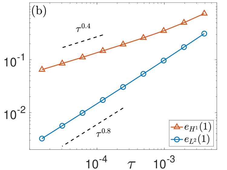
Figure 1: Errors in $L^{2}$- and $H^{1}$-norms of the EWI for the NLSE with singular potentials in 1D: (a) $\alpha=0.51$ and (b) $\alpha=0.76$

Next, we consider a 2D example with $\Omega=(-8,8)\times(-8,8)$ and $T=1/4$, and choose $\beta=-1$, $\sigma=1$ in Eq. 1. In this example, we study two kinds of singular potentials: (a) the Coulomb potential with $\alpha=1$ in Eq. 77, which is in $L^{2-}$; (b) the random potential generated in the Fourier space through Eq. 78 with

(80) $$\widehat{v}_{0,0}=1,\quad\widehat{v}_{\bm{l}}=\frac{\xi_{\bm{l}}}{|\bm{\mu_{l}}|},\quad(0,0)^{T}\neq\bm{l}\in\left\{-\frac{N_{\text{ref}}}{2},\cdots,\frac{N_{\text{ref}}}{2}-1\right\}^{2},$$

where $\xi_{\bm{l}}=\text{rand}(-1,1)+i\ \text{rand}(-1,1)$ with $\text{rand}(-1,1)$ returning a random number uniformly distributed in $[-1,1]$, and $N_{\text{ref}}=2^{9}$. The reference solution is obtained by the EWI using $\tau_{\text{e}}=10^{-5}$ and $h_{\text{e}}=2^{-5}$ in both directions.

The numerical results are presented in Fig. 2 (a) and (b) for the two potentials, respectively. In both cases, we see that the $L^{2}$-norm convergence is first-order and the $H^{1}$-norm convergence is half-order, corresponding well with our error estimates. We remake here that the convergence order reduction from $1$ to $1^{-}$ is hard to examine numerically.

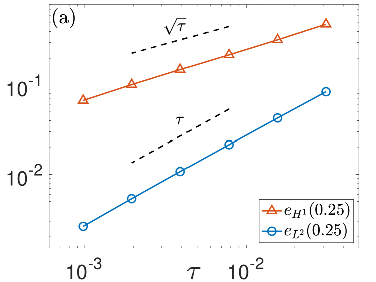
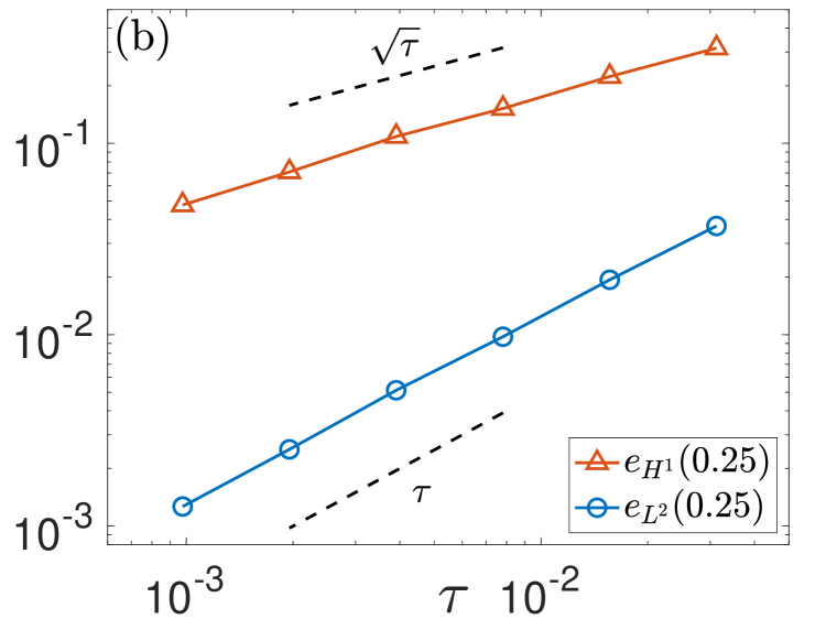
Figure 2: Errors in $L^{2}$- and $H^{1}$-norms of the EWI for the NLSE with $L^{2}$-potential in 2D: (a) Coulomb potential and (b) random potential

Then we conduct a 3D numerical experiment with $\Omega=(-8,8)^{3}$ and $T=1/8$, and set $\beta=1$, and $\sigma=1$ in Eq. 1. Two singular potentials of the form Eq. 78 are considered: (a) an $L^{3^{-}}$-potential with $\widehat{v}_{\bm{l}}=(1+|\bm{\mu_{l}}|^{2})^{-1}$ in Eq. 78, which has the same singularity as the Coulomb potential $-|\bm{x}|^{-1}$ (recalling that the Fourier transform of $|\bm{x}|^{-1}$ in $\mathbb{R}^{3}$ is $C|\bm{\xi}|^{-2}$); (b) an $L^{2}$-potential with $\widehat{v}_{\bm{l}}=(1+|\bm{\mu_{l}}|^{2})^{-0.76}$ in Eq. 78. The reference solution is computed by the EWI using $\tau_{\text{e}}=10^{-4}$ and $h_{\text{e}}=2^{-5}$ in all the three dimensions.

We plot the numerical results in Fig. 3, where first-order convergence in $L^{2}$-norm is observed for both the $L^{3^{-}}$-potential in (a) and the $L^{2}$-potential in (b). These results verify our error estimates, while, the convergence order reduction for $L^{2}$-potential in 3D stated in Theorem 2.2 is not observed, suggesting that first-order $L^{2}$-norm convergence might be extended to $L^{p}+L^{\infty}$-potential with $2\leq p\leq\frac{12}{5}$. In addition, the $H^{1}$-norm convergence is 0.85-order for $L^{3^{-}}$-potential, which is due to the smooth Gaussian initial data and the better regularity of the $L^{3^{-}}$-potential (which is in fact $H^{\frac{1}{2}-}$).

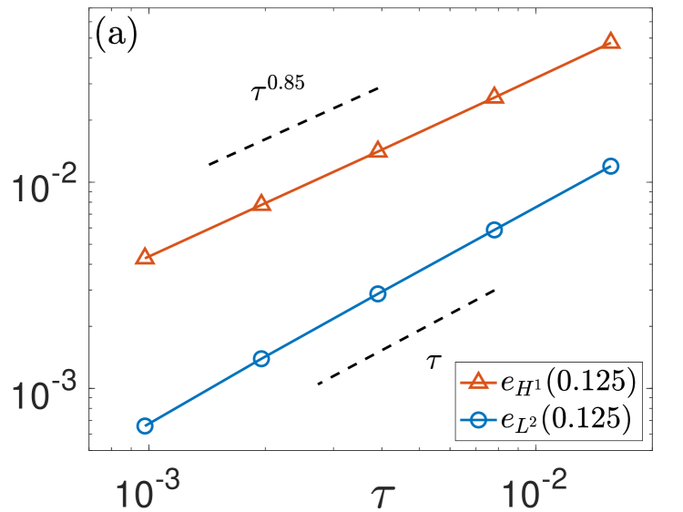
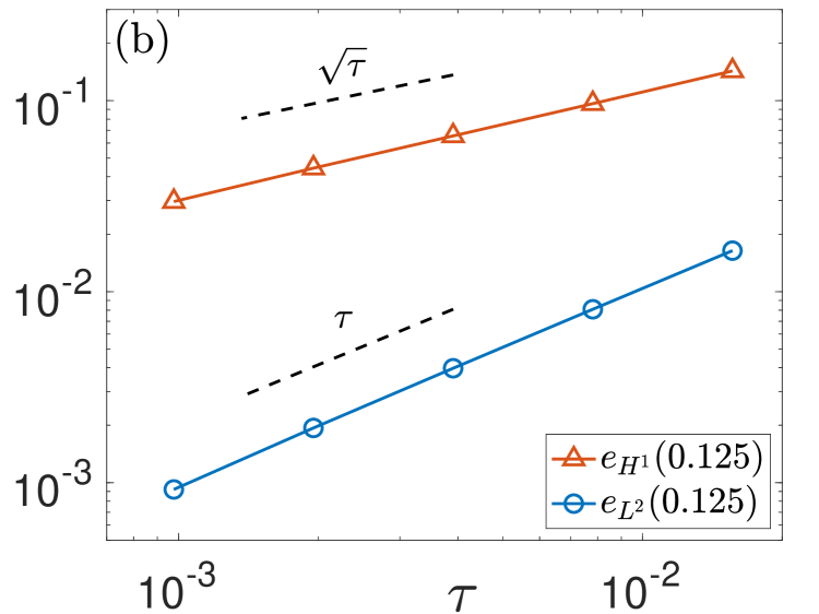
Figure 3: Errors in $L^{2}$- and $H^{1}$-norms of the EWI for the NLSE with singular potentials in 3D: (a) $L^{3^{-}}$-potential and (b) $L^{2}$-potential

Finally, we apply the EWI Eq. 4 to simulate the dynamics under four attractive Coulomb potentials in 2D, which is given by Eq. 6 with $\alpha=1$, $J=4$, $Z_{j}=-1$, and

$$x_{1}=(-1,0)^{T},\quad x_{2}=(1,0)^{T},\quad x_{3}=(0,1)^{T},\quad x_{4}=(0,-1)^{T}.$$

The initial datum is chosen as

$$\psi_{0}(\bm{x})=\phi(\bm{x}-\bm{x}_{0})e^{ix_{1}},\quad\bm{x}_{0}=(-4,2)^{T},\quad\bm{x}=(x_{1},x_{2})^{T}\in\Omega,$$

where $\phi$ is the unique positive radial (action) ground state of the stationary NLSE

(81) $$-\Delta\phi(\bm{x})+\omega\phi(\bm{x})-|\phi(\bm{x})|^{2}\phi(\bm{x})=0,\quad\bm{x}\in\mathbb{R}^{2},\quad\omega=3.$$

The initial set-up is illustrated in Fig. 4.

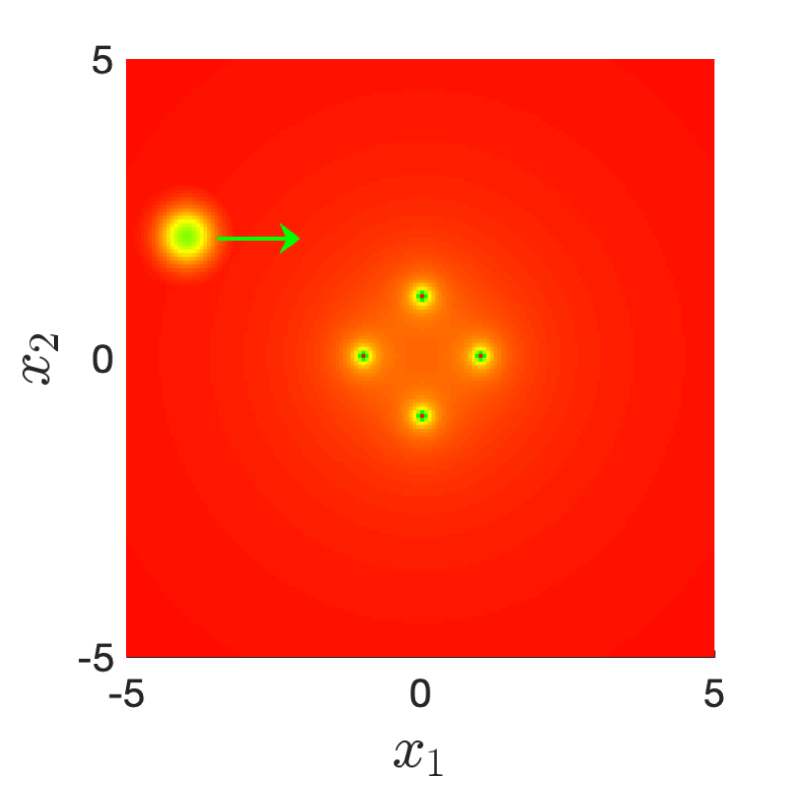
Figure 4: Illustration of the initial set up

In computation, we choose $\Omega=(-8,8)\times(-8,8)$ and $T=4$ with $\tau=10^{-4}$ and $h=2^{-5}$ for both directions. The density $|\psi(\bm{x},t)|^{2}$ at different time $t$ are exhibited in Fig. 5.

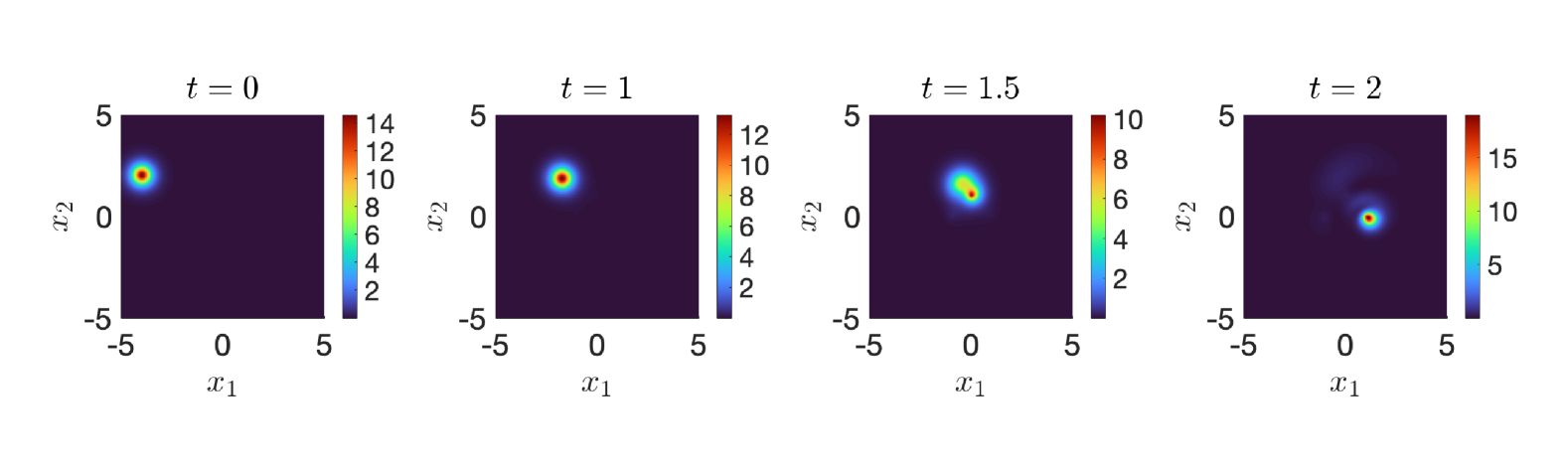
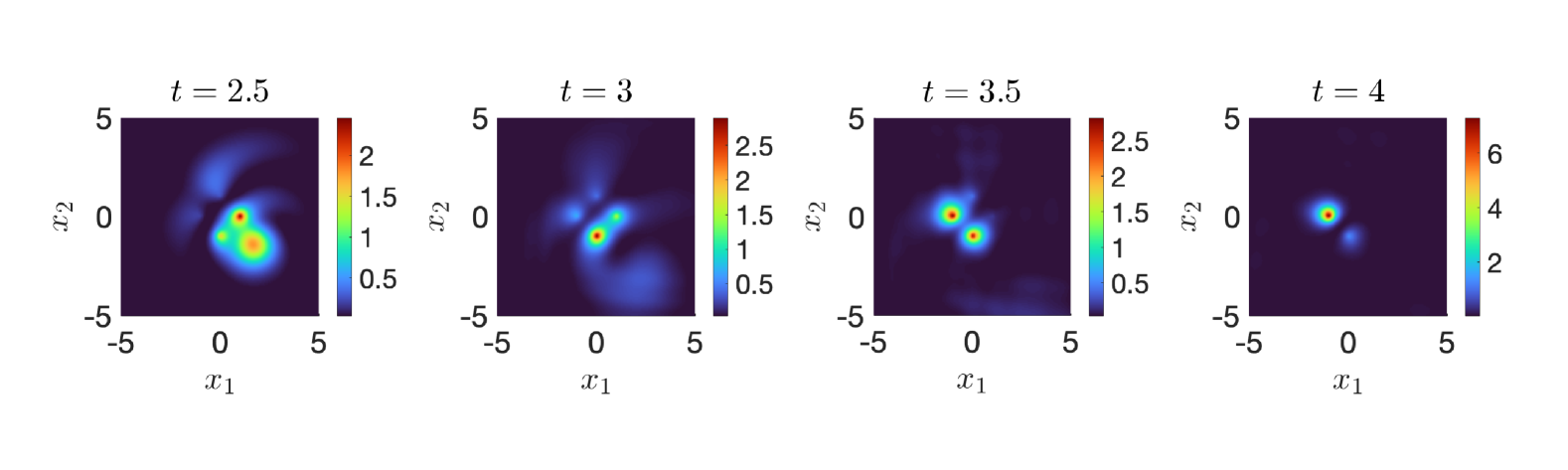
Figure 5: Plots of $|\psi(\cdot,t)|^{2}$ at different time $t$ for the dynamics under four Coulomb potentials in 2D

The numerical results demonstrate that the solitary wave initially moves to the right and becomes attracted to the upper Coulomb potential, subsequently visiting all four Coulomb centers in a clockwise sequence.

6 Conclusion

We analyzed a first-order EWI for the NLSE with the singular potential of $L^{p}$-type under $H^{2}$-initial data. We obtained convergence orders for $L^{p}$-potential with $2\leq p<\infty$ in 1D, 2D, and 3D. For $L^{2}$-potential, the EWI is almost first-order convergent in $L^{2}$-norm in 1D and 2D, while the convergence order is reduced to $\frac{3}{4}$-order in 3D. Under a stronger integrability assumption of $L^{p}$-potential with $p>\frac{12}{5}$ in 3D, the first-order $L^{2}$-norm convergence was proved. We also apply our results to the important cases of the inverse power potential. In particular, our results show that the EWI is optimally first-order convergent in $L^{2}$-norm under 3D Coulomb potential. Extensive numerical results in 1D, 2D, and 3D verified our error estimates and showed that they are optimal.

References

- [1] Y. Alama Bronsard, Y. Bruned, and K. Schratz, Low regularity integrators via decorated trees, 2022, arXiv:2202.01171.
- [2] P. W. Anderson, Absence of diffusion in certain random lattices, Phys. Rev., 109 (1958), pp. 1492–1505.
- [3] X. Antoine, W. Bao, and C. Besse, Computational methods for the dynamics of the nonlinear Schrödinger/Gross-Pitaevskii equations, Comput. Phys. Commun., 184 (2013), pp. 2621–2633.
- [4] W. Bao and Y. Cai, Mathematical theory and numerical methods for Bose-Einstein condensation, Kinet. Relat. Models, 6 (2013), pp. 1–135.
- [5] W. Bao and Y. Cai, Optimal error estimates of finite difference methods for the Gross-Pitaevskii equation with angular momentum rotation, Math. Comp., 82 (2013), pp. 99–128.
- [6] W. Bao, D. Jaksch, and P. A. Markowich, Numerical solution of the Gross-Pitaevskii equation for Bose-Einstein condensation, J. Comput. Phys., 187 (2003), pp. 318–342.
- [7] W. Bao, B. Lin, Y. Ma, and C. Wang, An extended Fourier pseudospectral method for the Gross-Pitaevskii equation with low regularity potential, East Asian J. Appl. Math., 14 (2024), pp. 530–550.
- [8] W. Bao, Y. Ma, and C. Wang, Optimal error bounds on time-splitting methods for the nonlinear Schrödinger equation with low regularity potential and nonlinearity, Math. Models Methods Appl. Sci., 34 (2024), pp. 803–844.
- [9] W. Bao and C. Wang, Error estimates of the time-splitting methods for the nonlinear Schrödinger equation with semi-smooth nonlinearity, Math. Comp., 93 (2024), pp. 1599–1631.
- [10] W. Bao and C. Wang, An explicit and symmetric exponential wave integrator for the nonlinear Schrödinger equation with low regularity potential and nonlinearity, SIAM J. Numer. Anal., 62 (2024), pp. 1901–1928.
- [11] W. Bao and C. Wang, Optimal error bounds on the exponential wave integrator for the nonlinear Schrödinger equation with low regularity potential and nonlinearity, SIAM J. Numer. Anal., 62 (2024), pp. 93–118.
- [12] S. Becker, N. Galke, R. Salzmann, and L. van Luijk, Convergence rates for the Trotter-Kato splitting, 2024, arXiv:2407.04045.
- [13] C. Besse, B. Bidégaray, and S. Descombes, Order estimates in time of splitting methods for the nonlinear Schrödinger equation, SIAM J. Numer. Anal., 40 (2002), pp. 26–40.
- [14] Y. Bruned and K. Schratz, Resonance-based schemes for dispersive equations via decorated trees, Forum Math. Pi, 10 (2022), e2, 76.
- [15] D. Burgarth, P. Facchi, A. Hahn, M. Johnsson, and K. Yuasa, Strong error bounds for Trotter and Strang-splittings and their implications for quantum chemistry, Phys. Rev. Res., 6 (2024), p. 043155.
- [16] R. Carles and C. Su, Scattering and uniform in time error estimates for splitting method in NLS, Found. Comput. Math., 24 (2024), pp. 683–722.
- [17] K. M. Case, Singular potentials, Phys. Rev., 80 (1950), pp. 797–806.
- [18] T. Cazenave, Semilinear Schrödinger Equations, Cour. Lect. Notes Math. 10, Courant Institute of Mathematical Sciences, New York, 2003.
- [19] E. Celledoni, D. Cohen, and B. Owren, Symmetric exponential integrators with an application to the cubic Schrödinger equation, Found. Comput. Math., 8 (2008), pp. 303–317.
- [20] H. J. Choi, S. Kim, and Y. Koh, Time splitting method for nonlinear Schrödinger equation with rough initial data in , J. Differential Equations, 417 (2025), pp. 164–190.
- [21] W. Choi and Y. Koh, On the splitting method for the nonlinear Schrödinger equation with initial data in , Discrete Contin. Dyn. Syst., 41 (2021), pp. 3837–3867.
- [22] L. Erdős, B. Schlein, and H.-T. Yau, Derivation of the cubic non-linear Schrödinger equation from quantum dynamics of many-body systems, Invent. Math., 167 (2007), pp. 515–614.
- [23] G. Fibich, The Nonlinear Schrödinger Equation: Singular Solutions and Optical Collapse, Springer, Cham, 2015.
- [24] W. M. Frank, D. J. Land, and R. M. Spector, Singular potentials, Rev. Mod. Phys., 43 (1971), pp. 36–98.
- [25] C. Gross and I. Bloch, Quantum simulations with ultracold atoms in optical lattices, Science, 357 (2017), pp. 995–1001.
- [26] P. Henning and D. Peterseim, Crank-Nicolson Galerkin approximations to nonlinear Schrödinger equations with rough potentials, Math. Models Methods Appl. Sci., 27 (2017), pp. 2147–2184.
- [27] M. Hochbruck and A. Ostermann, Exponential integrators, Acta Numer., 19 (2010), pp. 209–286.
- [28] L. I. Ignat, A splitting method for the nonlinear Schrödinger equation, J. Differential Equations, 250 (2011), pp. 3022–3046.
- [29] T. Jahnke and C. Lubich, Error bounds for exponential operator splittings, BIT, 40 (2000), pp. 735–744.
- [30] L. Ji, A. Ostermann, F. Rousset, and K. Schratz, Low regularity full error estimates for the cubic nonlinear Schrödinger equation, SIAM J. Numer. Anal., 62 (2024), pp. 2071–2086.
- [31] C. Lubich, On splitting methods for Schrödinger-Poisson and cubic nonlinear Schrödinger equations, Math. Comp., 77 (2008), pp. 2141–2153.
- [32] N. J. Mauser, Y. Wu, and X. Zhao, The cubic nonlinear Schrödinger equation with rough potential, 2024, arXiv:2403.16772.
- [33] K. Meetz, Singular potentials in nonrelativistic quantum mechanics, Il Nuovo Cimento (1955-1965), 34 (1964), pp. 690–708.
- [34] C. Nisoli and A. R. Bishop, Attractive inverse square potential, gauge, and winding transitions, Phys. Rev. Lett., 112 (2014), p. 070401.
- [35] A. Ostermann, F. Rousset, and K. Schratz, Error estimates at low regularity of splitting schemes for NLS, Math. Comp., 91 (2021), pp. 169–182.
- [36] A. Ostermann, F. Rousset, and K. Schratz, Error estimates of a Fourier integrator for the cubic Schrödinger equation at low regularity, Found. Comput. Math., 21 (2021), pp. 725–765.
- [37] A. Ostermann, F. Rousset, and K. Schratz, Fourier integrator for periodic NLS: low regularity estimates via discrete Bourgain spaces, J. Eur. Math. Soc., 25 (2023), pp. 3913–3952.
- [38] A. Ostermann and K. Schratz, Low regularity exponential-type integrators for semilinear Schrödinger equations, Found. Comput. Math., 18 (2018), pp. 731–755.
- [39] L. Pitaevskii and S. Stringari, Bose-Einstein Condensation and Superfluidity, Oxford University Press, 2016.
- [40] F. Rousset and K. Schratz, Resonances as a computational tool, Found. Comput. Math., DOI:s10208-024-09665-8.
- [41] J. M. Sanz-Serna, Methods for the numerical solution of the nonlinear Schrödinger equation, Math. Comp., 43 (1984), pp. 21–27.
- [42] M. Schreiber, S. S. Hodgman, P. Bordia, H. P. Lüschen, M. H. Fischer, R. Vosk, E. Altman, U. Schneider, and I. Bloch, Observation of many-body localization of interacting fermions in a quasirandom optical lattice, Science, 349 (2015), pp. 842–845.
- [43] E. Schrödinger, Quantisierung als eigenwertproblem, Annalen der Physik, 384 (1926), pp. 361–376.
- [44] S. Shao and L. Su, Nonlocalization of singular potentials in quantum dynamics, J. Comput. Electron., 22 (2023), pp. 930–945.
- [45] C. Sulem and P.-L. Sulem, The Nonlinear Schrödinger Equation: Self-focusing and Wave Collapse, Springer, 1999.
- [46] H. Yukawa, On the interaction of elementary particles, Prog. Theor. Phys. Suppl., 1 (1955), pp. 1–10.
- [47] X. Zhou, Y. Cai, X. Tang, and G. Xu, Accurate and efficient numerical methods for the nonlinear Schrödinger equation with Dirac delta potential, Calcolo, 60 (2023), Paper No. 57.