Policy Optimization Algorithms in a Unified Framework
Abstract
Policy optimization algorithms are crucial in many fields but challenging to grasp and implement, often due to complex calculations related to Markov decision processes and varying use of discount and average reward setups. This paper presents a unified framework that applies generalized ergodicity theory and perturbation analysis to clarify and enhance the application of these algorithms. Generalized ergodicity theory sheds light on the steady-state behavior of stochastic processes, aiding understanding of both discounted and average rewards. Perturbation analysis provides in-depth insights into the fundamental principles of policy optimization algorithms. We use this framework to identify common implementation errors and demonstrate the correct approaches. Through a case study on Linear Quadratic Regulator problems, we illustrate how slight variations in algorithm design affect implementation outcomes. We aim to make policy optimization algorithms more accessible and reduce their misuse in practice.
keywords:
policy optimization; ergodicity; reinforcement learning.1 Introduction
Policy optimization algorithms are fundamental in reinforcement learning. Unlike value learning methods, policy optimization algorithms directly learn the optimal policy, mapping states to actions. These algorithms are flexible, applicable to continuous actions and support stochastic policies, making them useful in various fields. Examples include game AI (Berner et al., 2019), robotic locomotion (Miki et al., 2022), chatbot fine-tuning (Ouyang et al., 2022), reasoning model training (DeepSeek-AI, 2025), robotic manipulation (Ibarz et al., 2021), character animation (Peng et al., 2018), nuclear fusion control (Degrave et al., 2022), and chip design (Mirhoseini et al., 2021).
The main goal of policy optimization algorithms is to search optimal policies for Markov Decision Processes (MDPs). MDPs deal with decision-making under uncertain state changes. Analyzing MDPs is challenging because of the complexity in stochastic processes and the subtleties of discount factors. The discount factors reflect real-world timing preferences and help stabilize learning algorithms but can complicate analysis and interpretation. A notable issue in research is the lack of clear distinction between discounted and average reward setups, which leads to confusion and errors in implementation.
Several studies investigate empirical implementation details and provide guidelines for policy optimization algorithms (Engstrom et al., 2019; Huang et al., 2023). However, there is a gap in the literature addressing the proper theoretical implementation of these algorithms, with a few exceptions (Thomas, 2014; Nota and Thomas, 2020; Wu et al., 2022). Thomas (2014) pointed out that several natural policy gradient algorithms for discounted objectives yield biased gradient estimates due to ignoring the discount factor. Nota and Thomas (2020) highlighted a similar issue in popular policy gradient algorithms, where the update direction is not a gradient of any objective function. Wu et al. (2022) demonstrated how to correctly derive policy gradient algorithms in a unified manner for various setups. The common issue relates to appropriately treating the discount factor in implementations. Despite this commonality, it is not obvious how these works are connected or how to systematically avoid potential mistakes when implementing other policy optimization algorithms. There is a need for a comprehensive guide that addresses these topics accessibly for those new to the field, helping demystify the complex terminology.
To properly implement policy optimization algorithms, it is crucial to correctly understand how they work. We propose an easy-to-follow framework that clarifies both the principles of deriving these algorithms and the correct way to implement them. We thus can reduce the chances of making mistakes during the implementation process or, at the very least, help people understand the purpose behind these algorithms better. Achieving this requires a clear and straightforward method for comprehending policy optimization algorithms.
In this paper, we develop a framework to make it easier to understand and connect various policy optimization algorithms. We focus on integrating different setups (discounted, total, and average rewards) and various algorithms, including policy iteration (Howard, 1960), policy gradient (Williams, 1992; Sutton et al., 1999), natural policy gradient (Kakade, 2001), trust region policy optimization (Schulman et al., 2015), and proximal policy optimization, specifically the PPO-clip version (Schulman et al., 2017). We use two main tools: a generalized concept of ergodicity and perturbation analysis. Ergodicity theory (Petersen, 1999) suggests that over the long term, the time averages of a stochastic process will match up with its space averages, given certain conditions. We expand on this idea of ergodicity to cover both discounted reward and average reward, making it possible to use space-based approaches and simplify the derivation of policy optimization algorithms. Perturbation analysis (Hinch, 1991) solves complex problems by starting with a simpler one and adjusting for small changes. This approach is useful for comparing policies and analyzing policy behaviors under perturbations (Cao, 2007). For both discounted and average reward setups, Cao (2007) derived policy iteration and policy gradient algorithms with a primary focus on policy performance comparison. We extend (Cao, 2007) beyond performance comparison and thus enable the derivation of more policy optimization algorithms such as natural policy gradient, TRPO, and PPO. Furthermore, Cao (2007) used different notations from the contemporary reinforcement learning convention, whereas we adopt a modern notation system that enhances readability.
Our contributions are threefold:
-
•
We introduce the concept of generalized ergodicity, simplifying the transition from varied complex time-based MDP formulations to one single unified space-based formulations.
-
•
Based on the space-based formulation, we adopt perturbation analysis (Cao, 2007; Wu et al., 2022) to revisit mainstream policy optimization algorithms and enhance theoretical understanding of these algorithms, which further help us easily extend existing algorithms, e.g., PPO-Clip and TRPO for deterministic policies.
-
•
With enhance understanding of the policy optimization algorithms, we discuss why existing algorithms are prone to incorrect implementations. We prescribe a guideline for correctly implementing policy optimization algorithms.
Our goal is to make the key aspects of different policy optimization algorithms clear to a wide audience. We hope that this paper clarifies their purpose and minimizes errors in implementation caused by misunderstandings. We share our results using a space-based approach and provide practical implementation guides in two tables (Table 1 and 2), serving as a convenient reference.
| quantity | expression |
|---|---|
| performance metric | |
| performance difference | |
| stochastic policy gradient | |
| stochastic policy curvature | |
| deterministic policy gradient | |
| deterministic policy curvature |
| quantity | discounted () | average |
|---|---|---|
| S-PG | ||
| D-PG | ||
| S-PCM | ||
| D-PCM |
2 Problem Setup
This section introduces the Markov Decision Process (MDP) setup. An MDP consists of a state space , an action space , a state transition probability , and a reward function , where and are states and is an action. The process starts with an initial state distribution . A control policy creates a sequence of states and actions, known as a trajectory , where each new state follows the transition probability .
The expected outcomes of trajectories under a policy are represented as . The policy can be either stochastic (i.e., ), or deterministic (i.e., ). We assume that the policy is parameterized by , allowing us to use and interchangeably. Following (Hernández-Lerma and Lasserre, 1996), we express both the summation over discrete and integral over continuous variables using the unified form for discrete , and for continuous .
The general policy optimization problem for MDPs is
which considers three different setups:
-
•
Discounted total reward, for
-
•
Undiscounted total reward
-
•
Long-run average reward
Each setup has its critical application scenarios:
-
•
Discounted. As the prevalent approach in Reinforcement Learning (RL), it reflects preferences of recent rewards to future rewards and help stabilize learning algorithms. However, the optimal policy depends on the discount factor , and tuning to achieve a desirable optimal policy often involves trial and error.
-
•
Total. This approach is suitable for tasks with a goal state. The MDP should have a terminal state, and at least one policy should lead to this state in a finite expected time. Episodic MDP tasks (finite time) are special cases, incorporating the time step into the state.
-
•
Average. This approach aims for sustained high performance and is common in classical dynamic programming, especially in engineering applications with queuing systems (Cao and Chen, 1997). It’s gaining interest in RL, as noted in (Sutton and Barto, 2020, Section 10.3 & 10.4). For effectiveness, it requires specific properties in the Markov chain, like ergodicity. For broader conditions, such as unichain or multichain, refer to Kallenberg (2002).
Three setups can be linked under specific conditions.
-
•
Discounted and Total Reward: Setting in results in , assuming the total reward is finite (i.e., a terminal state with zero reward is reachable). We will discuss these two setups together. We use the notation for the discounted reward setup, as the results from can easily apply to by setting .
-
•
Discounted and Average Reward: If becomes unbounded as , indicating cyclic behavior in the MDP, the average reward setup is more suitable. By multiplying by , making applicable, we derive , which is the consequence of the Abel theorem (Hernández-Lerma and Lasserre, 1996, Lemma 5.3.1). As a side note, the discounted sum is commonly understood as exponential averaging in signal processing, which also indicates that there is a connection between the discounted sum and time average.
-
•
Total and Average Reward: In the Stochastic Shortest Path (SSP) framework (Bertsekas, 2005, Chapter 7), the setups are connected. The total reward addresses transient behavior before reaching a goal state. In contrast, the average reward considers the goal state recurrent and seeks the long-term average reward per step. Under mild conditions in SSP, an optimal policy for the undiscounted total reward setup is also optimal for the average reward setup if the total reward MDP has a reset transition that reset the state after reaching goal states.
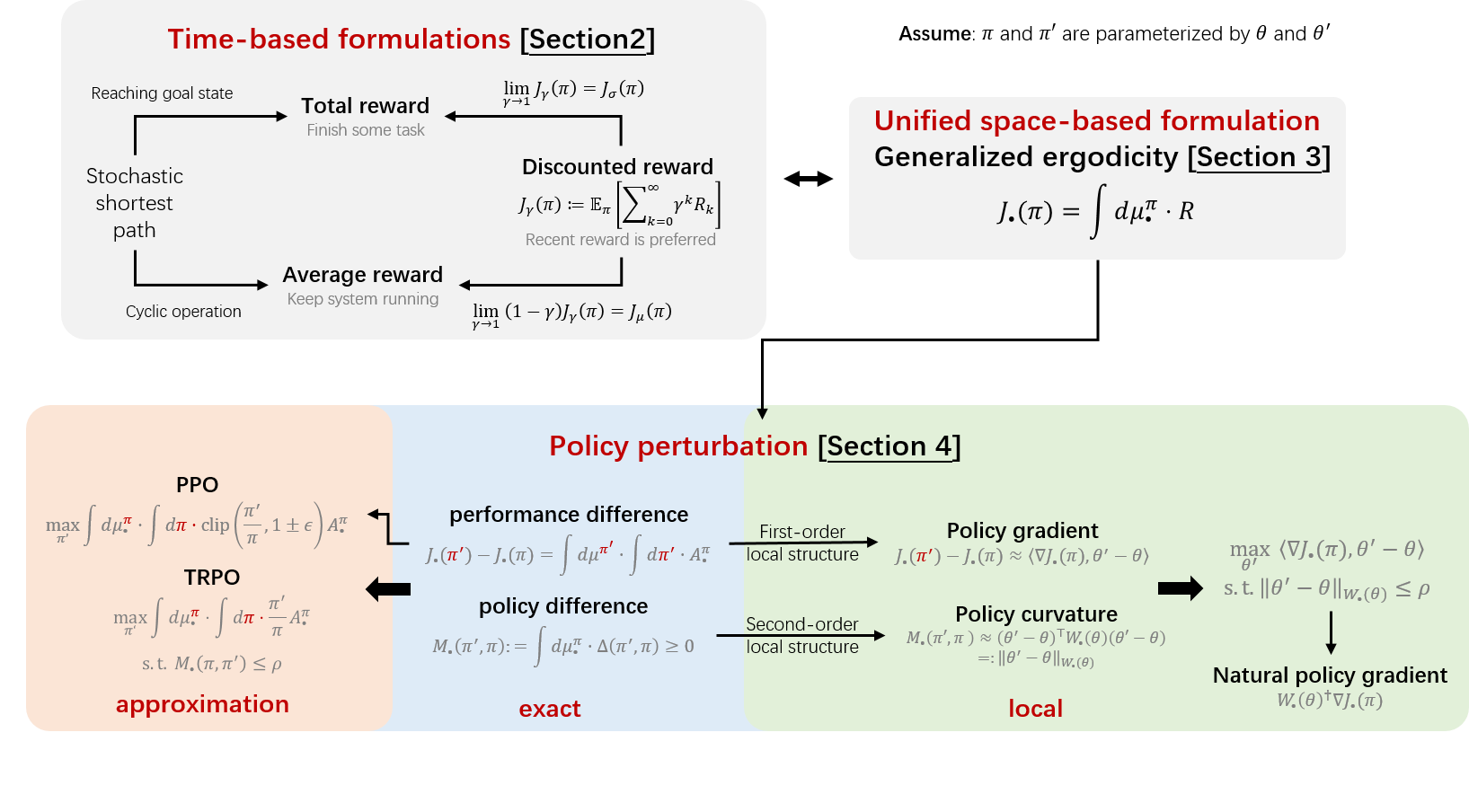
The three time domain setups present challenges in deriving straightforward policy optimization algorithms due to their complex nested structures from stochastic processes and the absence of a standardized approach, potentially leading to misuse of different setups (Thomas, 2014; Nota and Thomas, 2020; Wu et al., 2022). In Section 3, we introduce the concept of generalized ergodicity to unify these time-based setups into a single state-based framework. Following this, in Section 4, we use perturbation analysis to revisit and connect current popular policy optimization algorithms through this unified lens. Figure 1 previews our use of generalized ergodicity and perturbation analysis to clarify and link these algorithms. Our goal is to improve understanding and prevent common errors in implementing these algorithms, which is discussed in Section 5.
3 General Ergodicity
Ordinary ergodicity theory Petersen (1999) establishes the equality of time averages (averages over sample paths) and space averages (averages over the state space) under suitable conditions (e.g., recurrence). This enables converting results between time-based formulations, useful for Monte Carlo simulations, and space-based formulations, which simplify formula manipulation by dealing with random variables instead of stochastic processes. However, ergodicity is typically associated with the long-run average setup. In this work, we expand this concept to apply comprehensively to both long-run average and discounted setups.
3.1 Extension and Unification
Ergodicity theory claims that there exists a probability measure equating time and the space averages as below:
| (1) |
where is the invariant measure of the Markov chain induced by policy , i.e., . If exists, then .
We can extend to include discounted and total reward cases as . Eq. (1) then extends as
| (2) |
By combining eqn. (1) and eqn. (2), we establish a unified notation for as follows:
| (3) | ||||
We can interpret as an “averaging" measure. From Table 1, we can see that the MDP objective, performance difference, policy gradient (stochastic and deterministic), and policy curvature (stochastic and deterministic) are functions of and measured by . Note that the notation in , and should consistently used in the same equation. In other words, common expressions such as for stochastic policy gradient, for deterministic policy gradient, and for stochastic policy curvatures are not valid as both and appear in the same expression. We will further address the incorrectness and fixes in Section 5.
3.2 Application
Time-space conversion. Generalized ergodicity makes it easier to work with different time-based setups by combining them into a single space-based formula using a placeholder . This method is better for deriving formulae because it focuses on random variables instead of stochastic processes. After we come up with a space-based equation, we replace with specific setups. By looking at the ergodicity equations in eqn. (1) and (2), we can transform the equation back to a time-based format. This is useful for Monte Carlo simulations. We will demonstrate how this approach simplifies the development of various policy optimization algorithms in a coherent way and guarantees their correct implementation.
Transfer equations between setups. The generalized ergodicity lets us transfer equations between setups. For example, one found that the correct time-based implementation of policy gradient for the average reward is , then the unified ergodicity leads to following reasoning chain for deriving the counterpart in the discounted setup: 1) space-based gradient (average ergodicity) , 2) discounted space-based gradient (because of unified form) , and finally 3) discounted time-based gradient (because of time-space conversion) .
4 Revisit Policy Optimization
This section builds upon the unified space-based formulation using generalized ergodicity. We introduce a perturbation analysis approach to systematically derive well-known policy optimization algorithms within a unified framework.
4.1 Performance Difference and Exact Optimization
In this section, we simplify our notation by omitting from and . This helps avoid confusion without complicating the expressions.
Preliminaries. The state value function and the state-action value function are key for evaluating policy performance. They indicate the future cumulative reward for a current state and state-action pair. For discounted rewards, the state-action value is expressed as
while, with average rewards, it takes a different form:
Akin to , we adopt a unified notation to denote both and . This notation allows us to concisely express the value function and advantage function as follows:
Performance difference. In the context of general ergodicity, the objectives can be expressed as follows:
This equation indicates that the objectives represent the expected single-stage reward under a measure induced by policy . The advantage function , similar to , is a single-stage function. The expression represents the per-stage advantage of policy over . This leads one to guess whether the following performance difference formula is true:
| (4) |
As stated in (Schulman et al., 2015, eqn. (20)), this equation holds in a discounted setup111We show a state-based proof in the appendix. We can transfer the state-based result to the time-based version using ergodicity.:
| (5) |
Drawing on our discussion in the last section, we can generalize the relation to both average and discounted setups by applying generalized ergodicity, thereby verifing eqn. (4). We can also rigorously show why the extension to the average reward setup is correct. By Abel theorem (Hernández-Lerma and Lasserre, 1996, Lemma 5.3.1), for , . By multiplying both sides of eqn. (5) by and taking the limit as , we obtain222We prove in the appendix.
| (6) |
We thus rigorously derive the unified performance difference formula in eqn. (4).
Policy iteration. Since for each state, the policy difference formula leads to a simple method to find a better policy, that is, for every ,
| (7) |
This update is known as policy iteration Howard (1960). If is restricted to be a deterministic policy, the policy iteration is simplified to, for every , . The policy iteration scheme is straightforward as one only need to iterate between evaluating and finding the optimal of for each . Since for each state, this scheme ensures that the policy sequence from the iteration monotonically attains higher values.
Policy gradient. The performance difference formula can be further used to derive a policy gradient formula in a simple way333Sutton et al. (1999) developed proofs for stochastic policies in both discounted and average setup, and Silver et al. (2014) showed a proof for deterministic policy with discounted reward only. Wu et al. (2022) presented a simpler and more accessible proof using the perturbation method, which we include here for completeness.. Consider a policy parameterized by . According to the definition of gradient, the policy gradient is
| (8) |
For deterministic policies, we can derive
For stochastic policies, we can derive444As shown in (Wu et al., 2022), the proof can be extended to soft MDPs (Haarnoja et al., 2018; Geist et al., 2019; Mei et al., 2020) where the single stage reward involves an additional entropy-related term .
4.2 Approximate Policy Optimization
The performance difference formula requires accesses to instead of . The policy iteration greedily finds a better policy by omitting the weighting factor . Considering could lead to better policy updates. However, evaluating is costly and even intractable in general. Meanwhile, we have drawn samples from to calculate 555The discount factor should be considered for estimating quantities in the discounted setup. Neglecting leads to incorrect implementations as shown in the next section.. This motivates us to approximate the performance difference by substituting with , which leads to an approximate performance difference
| (9) |
The term is a function of random variables and , and its “expectation”666Note that is a probability distribution but is not. under their joint measure approximates the performance difference. This approximation is only valid when is close to . We discuss two popular approaches for keeping close to .
PPO-Clip from (Schulman et al., 2017). This method discourages from moving too far away from by clipping the policy ratio as follows
| (10) | ||||
While the original PPO-Clip approach is designed for stochastic policies, it faces issues with deterministic policies. In these cases, the ratio becomes problematic. For deterministic policies, the estimated policy difference is better represented as . A suitable PPO-Clip method for deterministic policies can be formulated as . This deterministic version is more challenging to implement than its stochastic counterpart.
Trust region policy optimization from (Schulman et al., 2015). Another approach to constrain is, while maximizing the approximate performance difference, adding explicit constraints to prevent from moving too far from . In particular, we introduce a metric function to measure the difference between two policies777The integral over is necessary as it allows a comprehensive evaluation of the policy differences. In particular, if we let , then will become the approximated performance difference.. The corresponding constrained optimization is formulated as
| (11a) | ||||
| s.t. | (11b) | |||
To ensure that is indeed a metric, we require that and the equation holds only when . Furthermore, we require to be invariant under different parameterization schemes and thus inherent to the policy space. Stochastic policies are probability distributions, and the Kullback–Leibler (KL) divergence is a natural choice:
Deterministic policies yields actions in a finite-dimensional vector space and a natural choice is the Euclidean distance between control actions (not controller parameters),
Remark 4.1.
For two stochastic policies and characterized by two Gaussian policies parameterized by and , the KL divergence is (Duchi, 2017, p.13). As , the policies and become deterministic policies, and , which is the policy difference measure for deterministic policies.
4.3 Simplified approximation and policy curvature
Eqn. (11) is challenging to solve due to the nonlinearity in both the objective and the constraint. We can simplify this by approximating the objective with a linear function in , expressed as . Similarly, we can approximate within a small region using a quadratic function as
This approximation scheme is feasible because and the equality only holds when . Using the quadratic approximation, we approximately solve the original trust region optimization in eqn. (11) as
| (12a) | ||||
| s.t. | (12b) | |||
Solving the KKT conditions in (12) leads to the update rule:
where the superscript stands for pseudo inverse since is not necessarily invertible. This update rule varies the stepsize depending on which requires solving an optimization problem. We can reduce the computation overhead by using a fixed stepsize
| (13) |
where is the stepsize. The update rule eqn. (13) is known as the natural policy gradient algorithm Kakade (2001). Since , we call the policy curvature. It shows the local policy space structure. If , the natural policy gradient simplifies to the policy gradient, overlooking the local structure.
We calculate the policy curvatures for both stochastic and deterministic policies. For stochastic policies, consider as a function of . The Taylor expansion of , up to the second order, is888Note that and since achieves its minimum value when . . Computing the Hessian matrix directly requires back-propagation twice. A more efficient formula is . We thus derive
For deterministic policies, the first-order Taylor expansion of at is . Therefore, . This allows us to approximate as . We thus derive
Remark 4.2 (TRPO and PPO).
Schulman et al., 2017 claimed that PPO-Clip is a simplified version of TRPO as it does not require solving the constrained optimization posed by TRPO. Apart from being simpler, PPO also surpasses TRPO in performance, a phenomenon not yet fully understood. Our derivations provide insights into why PPO is more effective. Specifically, PPO-Clip improves policy directly by optimizing the approximated performance difference within a small region. In contrast, TRPO practitioners approximate the original, highly nonlinear objective in eqn. (11) with a linear and a quadratic function for the objective and the constraint, respectively. While these simplifications lead to a more manageable optimization problem, they reduce the effectiveness of the approximation of the approximated performance difference in eqn. (9).
5 Issues in Implementation
Our generalized ergodicity framework prescribes policy optimization algorithms that match with . By applying ergodicity equations, we can transfer space-based equations to time-based equations, which allows us to implement these algorithms correctly for both discounted and average reward setups. Table 2 summarizes the corresponding formulae for implementation.
5.1 Incorrect Implementations
A number of previous works (Thomas, 2014; Nota and Thomas, 2020; Wu et al., 2022) pointed out that policy optimizations are often incorrectly executed, usually in a discounted reward setup.
Stochastic policies. The typical incorrect policy gradient and policy curvature are:
| (14) | ||||
| (15) |
However, these formulae can confuse users into thinking they should calculate expectations under the policy ’s distribution, leading to incorrect implementations as:
resulting in biased estimates for and . In particular, we can show that
and similarly, for policy curvature
Therefore, the incorrect implementations yield a measure over instead of .
Deterministic policies. The derivation resembles that of the stochastic policies. The typical incorrect policy gradient and policy curvature are:
| (16) | ||||
| (17) |
The corresponding incorrect implementations are:
resulting in biased estimates for and . We can show that
and similarly, for policy curvature
Therefore, the incorrect implementations yield a measure over instead of .
Summary of incorrect Implementations Because of misleading expressions discussed above, a number of incorrect implementations could be produced as listed in Table 3.
| name | expression | reason |
|---|---|---|
| hybrid gradient | mistake as | |
| hybrid natural gradient | mistake as | |
| hybrid natural hybrid gradient | both reasons above |
5.2 Correct implementations
In our space-based formulation, for discounted rewards, by substituting with , the equations for policy gradient and curvature become999Let ..
| stochastic policies | deterministic policies | |
|---|---|---|
Using the ergodicity for discounted setup, we derive the correct implementations, which include the discount factor as follows.
| stochastic policies | deterministic policies | |
|---|---|---|
These expressions align with the discounted total cost objective. In contrast, the incorrect methods directly use sample path sums for estimations, neglecting the discount factor in aggregating quantities along the sample path.
Remark 5.1.
Though incorrect implementations do not necessarily lead to significant errors, recognizing these nuances helps clarify the algorithms’ intended functionality and execution.
6 Case Studies
We discuss further how the algorithms are applied using case studies. We use the Linear quadratic regulator (LQR) problem as an example.
6.1 Linear quadratic regulator
The LQR problem is fundamental in optimal control theory. The state transition is linear in the state and the action , expressed as , where is the system matrix, is the control input matrix, and is the process noise. The single-stage cost101010We use cost instead of reward to align with the literature, e.g., (Bertsekas, 2005). The policy optimization problem minimizes the corresponding aggregated costs. is a quadratic function, expressed as . We consider all linear controllers , where is the controller parameter. The associated system dynamics can be simplified to , where .
In the discounted cost setup, the value function is quadratic . Here, is the solution to a Lyapunov equation . The state converges to a Gaussian distribution, i.e., , where solves another Lyapunov equation . For the discounted setup, we define to be the solution to the following Lyapunov equation . One can verify that and can be calculated by setting in the corresponding Lyapunov equations for and .
Define and . Plugging the performance difference equation in eqn. (4) into the LQR problem111111Both and are assumed to have no eigenvalues outside the unit circle on the complex plane to ensure and are bounded., we derive
| (18) | ||||
The policy gradient is then . The policy curvature can be directly computed from . The natural policy gradient is then .
6.2 Numerical Examples
We consider an LQR problem as , , , , , and linear controller parameterized by .
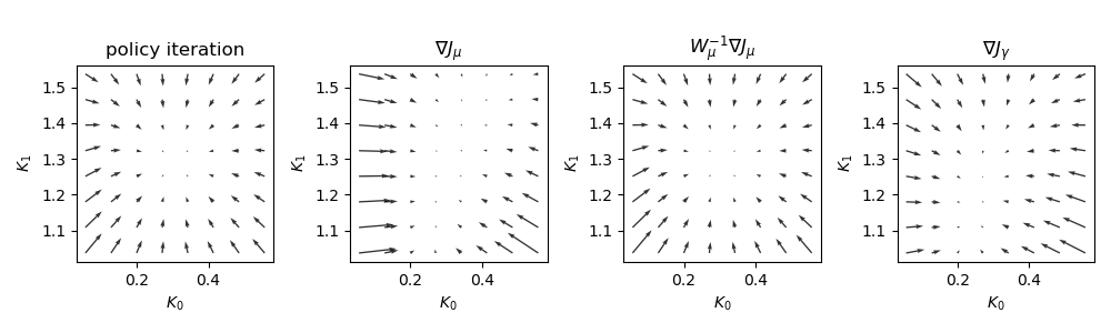
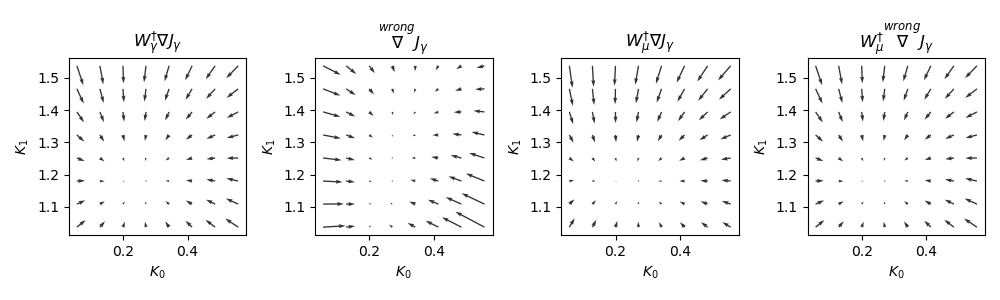
Vector field of update rules. We compare the policy update directions of a number of implementations, including policy iteration (for ), policy gradient (for both and ), natural policy gradients (for both and ), and three common incorrect implementations (see Table 3 in the appendix for a detailed description). We chose for scenarios involving discounted rewards. The generated vector field by these algorithms is depicted in Figure 2. Note that both the system dynamics and the discount factor influence the vector field landscape. Additional experiments in the appendix explore the relationship between and , revealing that slower systems require a larger discount factor to approximate the average reward setup effectively.
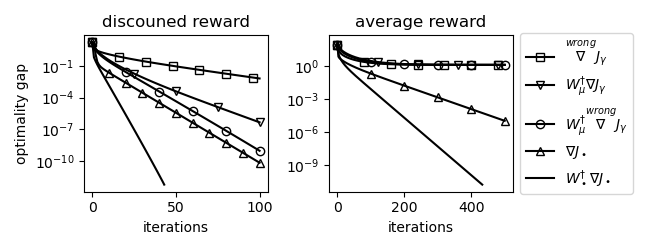
Optimality gap. We further investigate how different implementations impact performance, looking at both discounted and average cost setups. This included correct (using and ) and incorrect implementations (the three common ones as just mentioned). By using policy iteration as a benchmark for optimal cost, we calculated the optimality gap ( ) for these methods, shown in Figure 3. We tune the step sizes of different implementations for optimal convergence. In the discounted cost setup, while incorrect implementations converge, they do so more slowly due to limitations on step sizes. For the average cost setup, incorrect implementations failed to converge to the optimal solution.
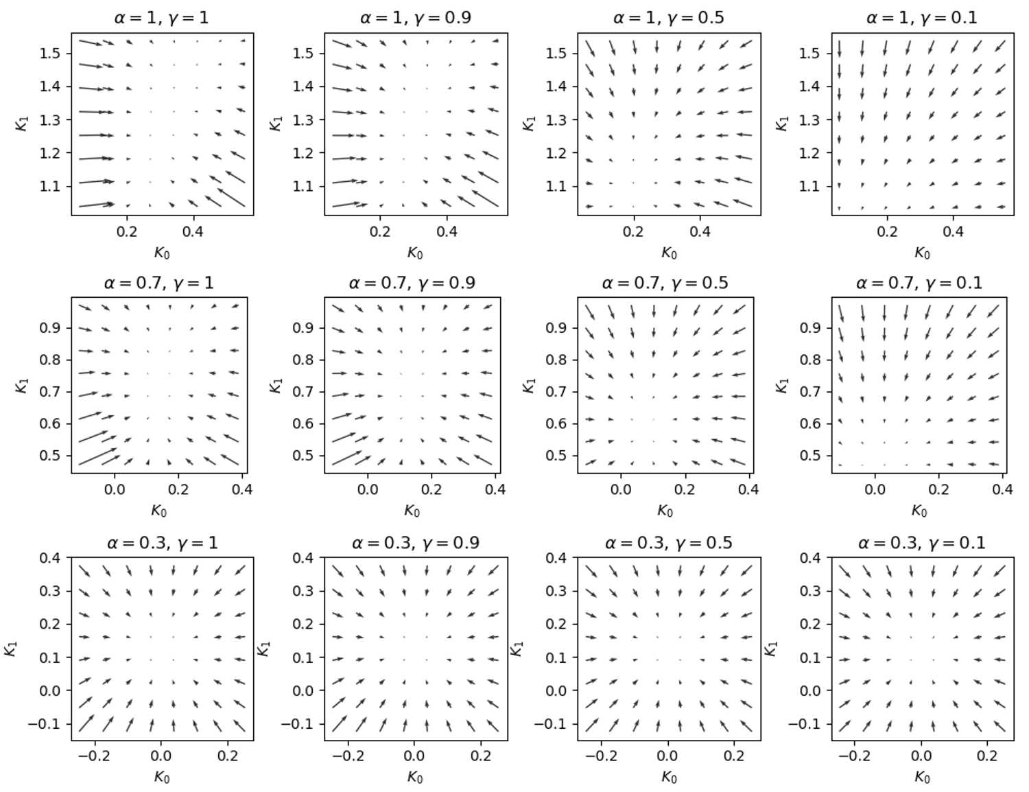
Impact of and MDP structure. We further investigate how the discount factor and the convergence speed of the Markov chain affect the vector field. Apart from using a parameterized system dynamics , other system parameters are the same as previous examples. Note that smaller yields faster system convergence in the absence of control input. Figure 4 shows the update directions with different system dynamics and discount factors. If the system dynamics converges at a fast rate (small ), the difference between using small and big is negligible.
7 Conclusions
We developed a generalized ergodicity theory to unify different MDP setups in a space-based formulation and leverage perturbation analysis to link existing popular policy optimization algorithms. We hope that this work fosters a comprehensive grasp of policy optimization algorithms and encourages correct implementations.
References
- Berner et al. [2019] Christopher Berner, Greg Brockman, Brooke Chan, Vicki Cheung, Przemysław “Psycho" Dębiak, Christy Dennison, David Farhi, Quirin Fischer, Shariq Hashme, Chris Hesse, Rafal Józefowicz, Scott Gray, Catherine Olsson, Jakub Pachocki, Michael Petrov, Henrique Pondé de Pinto, Jonathan Raiman, Tim Salimans, Jonas Schlatter, Jeremy annd Schneider, Szymon Sidor, Ilya Sutskever, Jie Tang, Filip Wolski, and Susan Zhang. Dota 2 with large scale deep reinforcement learning. arXiv preprint arXiv:1912.06680, 2019.
- Bertsekas [2005] Dimitri P. Bertsekas. Dynamic Programming and Optimal Control, volume I. Athena Scientific, Third edition, 2005.
- Cao [2007] Xi-Ren Cao. Stochastic Learning and Optimization: A Sensitivity-Based Approach. Springer Science & Business Media, 2007.
- Cao and Chen [1997] Xi-Ren Cao and Han-Fu Chen. Perturbation realization, potentials, and sensitivity analysis of markov processes. IEEE Transactions on Automatic Control, 42(10):1382–1393, 1997.
- DeepSeek-AI [2025] DeepSeek-AI. DeepSeek-R1: Incentivizing reasoning capability in LLMs via reinforcement learning, 2025. URL https://arxiv.org/abs/2501.12948.
- Degrave et al. [2022] Jonas Degrave, Federico Felici, Jonas Buchli, Michael Neunert, Brendan Tracey, Francesco Carpanese, Timo Ewalds, Roland Hafner, Abbas Abdolmaleki, Diego de Las Casas, Craig Donner, Leslie Fritz, Cristian Galperti, Andrea Huber, James Keeling, Maria Tsimpoukelli, Jackie Kay, Antoine Merle, Jean-Marc Moret, Seb Noury, Federico Pesamosca, David Pfau, Olivier Sauter, Cristian Sommariva, Stefano Coda, Basil Duval, Ambrogio Fasoli, Pushmeet Kohli, Koray Kavukcuoglu, Demis Hassabis, and Martin Riedmiller. Magnetic control of tokamak plasmas through deep reinforcement learning. Nature, 602(7897):414–419, 2022.
- Duchi [2017] John Duchi. Derivations for linear algebra and optimization, 2017. URL https://web.stanford.edu/˜jduchi/projects/general_notes.pdf.
- Engstrom et al. [2019] Logan Engstrom, Andrew Ilyas, Shibani Santurkar, Dimitris Tsipras, Firdaus Janoos, Larry Rudolph, and Aleksander Madry. Implementation matters in deep RL: A case study on PPO and TRPO. In International Conference on Learning Representations, 2019.
- Geist et al. [2019] Matthieu Geist, Bruno Scherrer, and Olivier Pietquin. A theory of regularized Markov decision processes. In International Conference on Machine Learning, pages 2160–2169, 2019.
- Haarnoja et al. [2018] Tuomas Haarnoja, Aurick Zhou, Pieter Abbeel, and Sergey Levine. Soft actor-critic: Off-policy maximum entropy deep reinforcement learning with a stochastic actor. In International conference on machine learning, pages 1861–1870, 2018.
- Hernández-Lerma and Lasserre [1996] Onésimo Hernández-Lerma and Jean B Lasserre. Discrete-Time Markov Control Processes: Basic Optimality Criteria. Springer Science & Business Media, 1996.
- Hinch [1991] E. J. Hinch. Perturbation Methods. Cambridge University Press, 1991.
- Howard [1960] Ronald A Howard. Dynamic Programming and Markov Processes. The MIT Press, Cambridge, MA, 1960.
- Huang et al. [2023] Shengyi Huang, Rousslan Fernand Julien Dossa, Antonin Raffin, Anssi Kanervisto, and Weixun Wang. The 37 implementation details of proximal policy optimization. In The ICLR Blog Track, 2023.
- Ibarz et al. [2021] Julian Ibarz, Jie Tan, Chelsea Finn, Mrinal Kalakrishnan, Peter Pastor, and Sergey Levine. How to train your robot with deep reinforcement learning: lessons we have learned. The International Journal of Robotics Research, 40(4-5):698–721, 2021.
- Kakade and Langford [2002] Sham Kakade and John Langford. Approximately optimal approximate reinforcement learning. In International Conference on Machine Learning, 2002.
- Kakade [2001] Sham M Kakade. A natural policy gradient. In Advances in Neural Information Processing Systems, 2001.
- Kallenberg [2002] L. C. M. Kallenberg. Classification Problems in MDPs, pages 151–165. Springer US, Boston, MA, 2002.
- Mei et al. [2020] Jincheng Mei, Chenjun Xiao, Csaba Szepesvari, and Dale Schuurmans. On the global convergence rates of softmax policy gradient methods. In International Conference on Machine Learning, pages 6820–6829, 2020.
- Miki et al. [2022] Takahiro Miki, Joonho Lee, Jemin Hwangbo, Lorenz Wellhausen, Vladlen Koltun, and Marco Hutter. Learning robust perceptive locomotion for quadrupedal robots in the wild. Science Robotics, 7(62):eabk2822, 2022.
- Mirhoseini et al. [2021] Azalia Mirhoseini, Anna Goldie, Mustafa Yazgan, Joe Wenjie Jiang, Ebrahim Songhori, Shen Wang, Young-Joon Lee, Eric Johnson, Omkar Pathak, Azade Nazi, Azalia Mirhoseini, Anna Goldie, Mustafa Yazgan, Joe Wenjie Jiang, Ebrahim Songhori, Shen Wang, Young-Joon Lee, Eric Johnson, Omkar Pathak, Azade Nazi, Jiwoo Pak, Andy Tong, Kavya Srinivasa, William Hang, Emre Tuncer, Quoc V. Le, James Laudon, Richard Ho, Roger Carpenter, and Jeff Dean. A graph placement methodology for fast chip design. Nature, 594(7862):207–212, 2021.
- Nota and Thomas [2020] Chris Nota and Philip S Thomas. Is the policy gradient a gradient? In International Conference on Autonomous Agents and Multiagent Systems, pages 939–947, 2020.
- Ouyang et al. [2022] Long Ouyang, Jeffrey Wu, Xu Jiang, Diogo Almeida, Carroll L. Wainwright, Pamela Mishkin, Chong Zhang, Sandhini Agarwal, Katarina Slama, Alex Ray, John Schulman, Jacob Hilton, Fraser Kelton, Luke Miller, Maddie Simens, Amanda Askell, Peter Welinder, Paul Christiano, Jan Leike, and Ryan Lowe. Training language models to follow instructions with human feedback. In Advances in Neural Information Processing Systems, pages 27730–27744, 2022.
- Peng et al. [2018] Xue Bin Peng, Pieter Abbeel, Sergey Levine, and Michiel Van de Panne. DeepMimic: Example-guided deep reinforcement learning of physics-based character skills. ACM Transactions On Graphics (TOG), 37(4):1–14, 2018.
- Petersen [1999] Karl E. Petersen. Ergodic Theory. Cambridge University Press, 1999.
- Schulman et al. [2015] John Schulman, Sergey Levine, Pieter Abbeel, Michael Jordan, and Philipp Moritz. Trust region policy optimization. In International Conference on Machine Learning, pages 1889–1897, 2015.
- Schulman et al. [2017] John Schulman, Filip Wolski, Prafulla Dhariwal, Alec Radford, and Oleg Klimov. Proximal policy optimization algorithms. arXiv preprint arXiv:1707.06347, 2017.
- Silver et al. [2014] David Silver, Guy Lever, Nicolas Heess, Thomas Degris, Daan Wierstra, and Martin Riedmiller. Deterministic policy gradient algorithms. In International Conference on Machine learning, pages 387–395, 2014.
- Sutton and Barto [2020] Richard S Sutton and Andrew G Barto. Reinforcement Learning: An Introduction. MIT Press, 2nd edition, 2020.
- Sutton et al. [1999] Richard S Sutton, David A McAllester, Satinder P Singh, and Yishay Mansour. Policy gradient methods for reinforcement learning with function approximation. In Advances in Neural Information Processing Systems, pages 1057–1063, 1999.
- Thomas [2014] Philip Thomas. Bias in natural actor-critic algorithms. In International Conference on Machine Learning, pages 441–448, 2014.
- Williams [1992] Ronald J Williams. Simple statistical gradient-following algorithms for connectionist reinforcement learning. Machine Learning, 8(3):229–256, 1992.
- Wu et al. [2022] Shuang Wu, Ling Shi, Jun Wang, and Guangjian Tian. Understanding policy gradient algorithms: A sensitivity-based approach. In International Conference on Machine Learning, pages 24131–24149, 2022.
Appendix A Proofs
A.1 Proof of
Direct computation yields
| (19) | ||||
A.2 Proof of Performance Difference
Schulman et al. [2015, eqn. (20)] showed that
Kakade and Langford [2002] presented another earlier version of the proof. Both Schulman et al. [2015] and Kakade [2001] derived the result in a time-based formulation. We present a proof for the space-based version:
We consider the vector-based form of Bellman equations for discounted-reward MDPs:
where and are interpreted as functions of state and is operator on these functions121212If one assumes a finite state space and a finite action space, and are vectors, is a matrix, and the Bellman equation is a linear equation in .. We can derive
Subtracting on both sides, we obtain
Since , we derive
Writing the equation for each component , we derive
This completes the proof.