Adaptive sparse variational approximations for Gaussian process regression
Abstract
Accurate tuning of hyperparameters is crucial to ensure that models can generalise effectively across different settings. In this paper, we present theoretical guarantees for hyperparameter selection using variational Bayes in the nonparametric regression model. We construct a variational approximation to a hierarchical Bayes procedure, and derive upper bounds for the contraction rate of the variational posterior in an abstract setting. The theory is applied to various Gaussian process priors and variational classes, resulting in minimax optimal rates. Our theoretical results are accompanied with numerical analysis both on synthetic and real world data sets.
Keywords: variational inference, Bayesian model selection, Gaussian processes, nonparametric regression, adaptation, posterior contraction rates
1 Introduction
A core challenge in Bayesian statistics is scalability, i.e. the computation of the posterior for large sample sizes. Variational Bayes approximation is a standard approach to speed up inference. Variational posteriors are random probability measures that minimise the Kullback-Leibler divergence between a suitable class of distributions and the otherwise hard to compute posterior. Typically, the variational class of distributions over which the optimisation takes place does not contain the original posterior, hence the variational procedure can be viewed as a projection onto this class. The projected variational distribution then approximates the posterior. During the approximation procedure one inevitably loses information and hence it is important to characterize the accuracy of the approach. Despite the wide use of variational approximations, their theoretical underpinning started to emerge only recently, see for instance Alquier and Ridgway (2020); Yang et al. (2020); Zhang and Gao (2020a); Ray and Szabó (2022).
In a Bayesian procedure, the choice of prior reflects the presumed properties of the unknown parameter. In comparison to regular parametric models, where in view of the Bernstein-von Mises theorem the posterior is asymptotically normal, the prior plays a crucial role in the asymptotic behaviour of the posterior. In fact, the large-sample behaviour of the posterior typically depends intricately on the choice of prior hyperparameters, so it is vital that these are tuned correctly. Many Bayesian procedures for model selection/hyperparameter tuning have been proposed and studied over the years. The two classical approaches are hierarchical and empirical Bayes methods. In hierarchical Bayes the tuning hyperparameters are endowed with another layer of prior resulting in a multi-layer, hierarchical prior distribution, while in empirical Bayes the hyperparameters are estimated empirically and plugged into the posterior; see for instance the monograph Ghosal and van der Vaart (2017) for an overview of these methods. However, these classical methods, especially in more complex models and large data sizes, can be numerically very slow. In this paper we propose a method for variational hyperparameter tuning that speeds up the computations and provides reliable inference, as supported both by theory and empirical evidence.
Although our approach can be more generally applied, we mainly focus on sparse variational approximations for Gaussian process (GP) posteriors in the nonparametric regression model. We consider as examples both the inducing variable approach proposed by Titsias (2009b) and a standard mean-field variational approach for approximating the posterior. This article extends a line of research in Nieman et al. (2022, 2023), where minimax convergence rates and reliable uncertainty quantification were derived for the variational posteriors. In these papers, however, it was assumed that the regularity of the underlying, data-generating function is known and the optimal tuning of the procedures heavily depended on it. In practice such information is usually not available, so here, in contrast, we modify the approximation scheme in such a way that the knowledge of the true regularity is no longer required. Hence, our procedure provides data-driven, adaptive inference on the unknown regularity classes.
Related literature.
Adaptive contraction rates for variational methods were first studied for tempered posteriors, where in Bayes’ rule the likelihood is raised to a power , diminishing its importance. In Chérief-Abdellatif and Alquier (2018) convergence rates were derived for mixture models, discussing also model selection using a regularised evidence lower bound (ELBO) criterion. In subsequent work, Chérief-Abdellatif (2019) takes a similar approach in a more general setting with discrete model selection parameter. For standard posterior distributions Zhang and Gao (2020a) have derived optimal contraction rate guarantees for mean-field variational approximation of hierarchical sieve priors in context of the many normal means model and later extended the results to more general high-dimensional settings in Zhang and Gao (2020b). Recently, an adaptive variational approach was proposed in Ohn and Lin (2024), by considering a mixture of variational approximations of the individual models. However, none of the present papers addresses the Gaussian process regression model and the investigated variational algorithms are also different than the ones we focus on.
Contributions.
Below is a short overview of our results.
-
–
We start by comparing various variational approaches for data driven tuning of the hyperparameter.
-
–
Then we derive contraction rate results for general (discrete mixture) hierarchical priors in context of the nonparametric regression model and show that the proposed variational approximation inherits the contraction rate under a condition on the Kullback-Leibler divergence between these measures.
-
–
We apply these general results for Gaussian process priors using two different type of variational classes, i.e. inducing variable methods and a mean-field type approximation. We derive minimax rate adaptive contraction over a range of Sobolev-type regularity classes.
-
–
Our theoretical results are accompanied with numerical analysis, considering both synthetic and real world data sets.
Organization of the paper.
In Section 2 we review variational Bayes methods and introduce a variational approach that we later show to be adaptive on the regularity of the truth. The notation is tailored to the nonparametric regression setting but the framework is general. Next, in Section 3, general contraction rate theorems on hierarchical and variational posteriors in the nonparametric regression model are given. The theory is applied in concrete examples in Section 4, including different variational methods and priors. Beside theoretical guarantees also numerical results are provided. All proofs and supporting lemmas are given in the subsequent appendix.
2 Model selection with variational Bayes
We consider the nonparametric regression model, where the goal is to infer a function from data
| (1) |
The domain is a subset of , and we assume random design, meaning that are i.i.d. from some distribution on . In our theory the common variance of the errors is assumed known, but later on we also demonstrate empirically that it can be estimated variationally.
In the Bayesian framework one endows the functional parameter with a prior distribution. We will consider Gaussian process priors constructed using a covariance kernel . Such priors typically rely on a collection of scaling or tuning hyperparameters , which, especially in high-dimensional and nonparametric settings, substantially influence the behaviour of the corresponding posterior. The optimal choices of these hyperparameters rely on the characteristics of the underlying truth . Since this information is typically not available, in practice data-driven choices are considered. A fully Bayesian approach is to endow the hyperparameter with a prior , resulting in a hierarchical prior in the form
where the hyper-prior can be a density or a probability mass function. The prior is also called a mixture (in our case a mixture of Gaussian processes). The hierarchical posterior corresponding to this prior is given by Bayes’ rule
| (2) |
where denotes the Gaussian product likelihood in the nonparametric regression model, and are the respective vectors of observations in (1). Along the same lines we denote by the posterior corresponding to the prior . Such hierarchical Bayesian procedures are widely used in the literature, however, especially for complex, high-dimensional models they face computational challenges. This is also the case in hierarchical Gaussian process regression. Hence in order to scale up the procedure the posterior is approximated by a distribution that is easier to compute.
In the variational approach the first step is to set the variational class, on which the posterior is projected. Let us consider a collection of variational classes indexed by the same hyperparameter . The variational approximation is then defined by projecting the hierarchical posterior onto the class , i.e.
where whenever the integral is well-defined. Recall that using (2) the KL-divergence can be rewritten in the form
where the ‘evidence lower bound’ function is defined as
| (3) |
Hence, as is well known, minimizing the KL-divergence is equivalent with maximizing the ELBO function. For each hyperparameter value , this results in an approximation of the hierarchical posterior . We choose among these approximations the one which minimizes the KL-divergence or equivalently maximizes the ELBO, i.e., we estimate as maximiser of
| (4) |
For computational reasons and to keep the presentation of the results clean, we optimize the hyperparameter only over a discrete, finite index set . As is made explicit in the notation, we allow for this set to change or grow with the number of observations. Our results may be extended to the case of non-discrete hyperparameters, e.g. continuous hyper-priors , using the idea of likelihood transformation in Donnet et al. (2018) and Rousseau and Szabo (2017).
To summarise, the variational approximation to the hierarchical posterior is the distribution
| (5) |
where
| (6) |
An alternative objective function, proposed in e.g. Titsias (2009b) and Hensman et al. (2013), is the evidence lower bound that does not involve the hierarchical prior , but with fixed hyperparameter ,
Maximizing the above function over is equivalent to minimizing the Kullback-Leibler divergence between the variational class and the posterior , i.e.
This objective can be maximised both over and , but since the objective function changes with , the two steps cannot be merged into one as before in (5). However, if the prior distributions , are all mutually singular, there is a simple relationship between the two ELBO objective functions, i.e.
| (7) |
As a consequence the variational posterior can also be obtained by maximising penalized by the log-hyper-prior density. In case the hyper-prior is the uniform distribution on , the two ELBOs are constant shifts of each other.
We argue, however, that this function is less natural for selecting the hyperparameter than the previous function in (4): note that
| (8) |
Therefore, maximizing the evidence lower bound over the hyperparameter is not equivalent to minimizing the KL-divergence due to the dependence of the log-evidence term in (8) on . Nevertheless, the relation (7) shows that the two ELBO-optimisations over are equivalent if in addition to the mutual singularity the hyper-prior is a uniform distribution. Any other choice of the hyper-prior gives the maximiser of (7) the interpretation of a regularised version of the maximiser of . See also Section 4 in Zhang and Gao (2020a), who start from the evidence lower bound given in (7).
3 Oracle rate with variational Gaussian processes
In this section we derive oracle contraction rates for the variational approximation of Gaussian process mixtures under general conditions. Then, in the next section we provide examples where the variational Bayes approach achieves the minimax adaptive contraction rates for various choices of GP priors, based on these general results. Since the variational approximation aims to mimic the behaviour of the hierarchical posterior, we start by deriving theoretical guarantees for this fully Bayesian approach. Since, to deal with the variational approach, we need tighter control on the tail behaviour of the hyper-posterior , we do not follow standard techniques (as in e.g. de Jonge and van Zanten (2010); Arbel et al. (2013)), but use an argument via empirical Bayes, as developed in Szabó et al. (2013); Rousseau and Szabo (2017).
Since our focus is on GP approximations, for computational and analytical convenience we tailor our conditions to centered GP priors with covariance kernel and discrete hyper-priors on , i.e. we study mixtures of the form
For each value of the hyperparameter we associate to the conditional prior a rate defined as the solution to
| (9) |
where is a large positive constant to be specified later. Under some mild additional assumptions, one can show that is the contraction rate of the posterior (this follows from the theory below applied to ). Under the conditions below we prove that the hierarchical posterior distribution contracts at the rate
where is a sequence tending to infinity arbitrarily slowly and is a threshold which ensures is bounded from below. One can view this rate as the oracle one, i.e. the best rate attained by any of the models/priors. In the next section we provide several examples where this oracle rate is minimax adaptive over a scale of Sobolev regularity classes.
The contraction rate of the posterior distribution is measured in the norm of , but in the proof we also use a standard testing argument, built on the empirical norm . In order to compare these two, we introduce the following regularity condition on the Gaussian process prior. Consider for any the Karhunen-Loève expansion of the Gaussian process with law ,
| (10) |
where denotes the eigenbasis of the covariance kernel that defines , and are the square roots of the eigenvalues. We require that the suprema of the eigenfunctions increase at most at a polynomial rate. That is, we assume there exist and such that
| (11) |
This condition is used together with a tail bound for the prior given below. Note that (11) is a mild assumption which is satisfied for example by the standard Fourier basis with . For a general kernel, the eigenfunctions may depend on the hyperparameter(s), in which case the results below still hold if the inequality (11) is valid uniformly for all in .
Given a function , we denote its tail (in the spectral domain) by
For with as in condition (11), suppose that
| (12) |
For the prior we require a similar tail condition:
| (13) |
These assumptions are used to compare the empirical norm used for testing with the norm on in which we measure the contraction rate (recall the definition of in (9)). Loosely speaking, we compare the two norms for functions projected onto the basis and handle the tail behaviour with the above upper bounds. We verify these assumptions in several examples of regularity classes and priors under some conditions depending on the parameter .
Furthermore, we assume that there exists a function such that for any , and all sufficiently small ,
| (14) |
This condition is used to refine the metric entropy bound implied by (9) in order to construct hypothesis tests whose error is sufficiently small.
Lastly, we impose a condition on the hyper-prior . We define the subset of ‘good’ hyperparameters as
| (15) |
and assume that the hyper-prior puts sufficient amount of mass on each element of this set, i.e.
| (16) |
The above condition on the hyper-prior is natural, and moreover very mild, as it only requires that at least an exponentially small mass is put on the elements . It is satisfied for a wide range of distributions, including the uniform distribution on a set that does not grow too fast with . Furthermore, we denote by the expectation of the data in the model (1). We are now in a position to present the main result on contraction for the mixture posterior.
Theorem 1
Note that the above theorem implies that the hierarchical posterior contracts at the rate around the true parameter , as the sequence in the definition of is arbitrary slow. In fact, the result is slightly stronger as it derives an exponentially fast convergence on a large event .
The proof of the theorem follows the lines of Rousseau and Szabo (2017) adapted to our specific setting. We start by showing that the maximum marginal likelihood estimator (MMLE)
| (17) |
belongs to the set of optimal hyperparameters with probability tending to one. This implies as an ancillary result that the MMLE empirical Bayes posterior
| (18) |
achieves the optimal oracle rate ; see Theorem 7 below. Furthermore, under the assumption that the set of optimal hyperparameters receives a sufficiently large prior mass (16) the hierarchical posterior also attains the same oracle contraction rate . The details are given in Section A.3.
Next we investigate the variational approximation of the hierarchical posterior given in (5).
Theorem 2
In addition to the conditions of Theorem 1, assume that there exists and such that and
| (19) |
Then there exists such that
The theorem states that under Condition (19), the variational posterior with the empirical hyperparameter maximizing the ELBO function in (6) has the same rate of contraction as the hierarchical posterior. As seen in the examples below, Condition (19) is mild. It basically requires that there is at least one hyperparameter amongst the ”good ones” in such that the variational class is sufficiently close in Kullback-Leibler divergence to the corresponding posterior distribution. The proof is deferred to Section A.4.
In the literature various, related conditions to (19) were considered. Recalling (8), note that
Assuming that this upper bound is of the order is similar to e.g. condition (C4) in Zhang and Gao (2020a) for variational posteriors and the assumptions in Theorem 2.4 of Alquier and Ridgway (2020) for tempered variational posteriors.
4 Examples
In this section we apply the main result on variational GP contraction to two specific variational Bayes methods.
The data-generating true function is assumed to belong to a -Sobolev type ball
i.e., its Sobolev norm is bounded by . We call the variational posterior adaptive if for , for some subset ,
as , where is an arbitrary sequence tending to infinity. We show through several examples below that various choices of priors and variational classes can result in adaptive contraction rates. First we consider the inducing variable methods introduced in Titsias (2009a) for polynomially and exponentially decaying eigenvalues of the prior covariance kernel. Then we also study a mean-field approximation by taking a mixture of truncated GPs as the hierarchical prior and truncated, mean-field GPs as the variational class.
4.1 Inducing variables approximations
First we consider the inducing variable variational approximations for GP regression introduced by Titsias (2009a). The idea is to compress the information possessed by the posterior into variables , which in turn will reduce the computational complexity of the method. The inducing variables are taken to be linear functionals of the parameter , hence possesses an -dimensional Gaussian distribution and is a Gaussian process. Then endowing with a Gaussian distribution with mean and variance and integrating out the conditional distribution results in a class of Gaussian processes indexed by and . The mean and covariance functions of the inducing GPs are of the form
where denotes the covariance kernel of the prior, and the covariance matrices (implicitly also dependent on ) corresponding to and the vector . We use this class of GPs as our variational class, i.e. we take
| (20) |
where denotes the Gaussian distribution with mean and covariance .
Various choices of inducing variables can be considered. Here we focus on the population and empirical spectral features inducing variables. In the population spectral features method we take , as inducing variables, where denotes the th eigenfunction of the prior covariance kernel . The computational complexity of this approach is , substantially reducing the computational time. However, this approach requires the explicit knowledge of the eigenfunctions of the prior GPs, which are often not available analytically. The empirical version of this method is called the sample spectral features variational method, where the inducing variables are defined as , where is the -th principal vector of the prior covariance matrix with entries . One can see that the covariance kernel is replaced with the sample covariance matrix and the eigenfunctions with the eigenvectors in this approach. This requires computation of the first principal components and the corresponding eigenvalues, which makes the procedure slower. But it is also more widely applicable than the population features, because it does not require an explicit expression for the eigenfunctions . In practice the are computed via Lanczos iteration or conjugate gradient descent, see for instance Gardner et al. (2018); Wenger et al. (2022); Stankewitz and Szabó (2024).
For fixed , the variational posterior can be determined analytically in terms of the data and covariances , , which can be computed exactly or numerically depending on the choice of inducing variables. For non-adaptive variational approximations the theoretical properties have been studied in Burt et al. (2020); Nieman et al. (2022).
Below we consider two of the arguably most standard eigenvalue structures, i.e. polynomially and exponentially decaying eigenvalues for the GP priors.
4.1.1 Polynomially decaying eigenvalues – tuning the exponent
First we investigate priors with polynomially decaying eigenvalues of the form
| (21) |
where are i.i.d. standard normal, is an orthonormal basis satisfying condition (11) for some , is the dimension of the covariate vectors , and is the regularity of the prior. Several priors possess such eigenstructure, including the Matérn kernels and the Riemann-Liouville processes (including integrated Brownian motions). Here the form of the prior closely matches the structure of the smoothness class, and for the original posterior contracts at the minimax rate around . In Nieman et al. (2022) it was shown that the variational posterior using either population or empirical spectral features inducing variables, contracts at this rate (albeit with respect to the Hellinger distance) provided that the number of inducing variables exceeds . Here we extend these results to data driven tuning of the hyperparameter and derive rates with respect to the stronger -norm instead of Hellinger distance. We consider the variational class in (20) with the smallest integer larger than .
We optimize the hyperparameter over the set
for fixed . We assume that for a . We consider a uniform discrete prior on .
Corollary 3
The proof of the corollary is deferred to Section B.1 in the Appendix.
As an example of these theoretical findings we consider a simulated data set of observations generated as
| (22) |
where
| (23) |
and form the real Fourier basis on rescaled to be orthonormal with respect to the uniform distribution. The function almost has Sobolev smoothness in the sense that for all . We take the prior defined in (21), and using the ELBO with population spectral features we estimate by and correspondingly take . In Figure 1 we show and the mean and pointwise credible regions of the variational posterior with variationally tuned . The credible regions nicely cover the true everywhere except for some of the points where it changes direction.
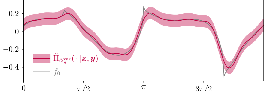
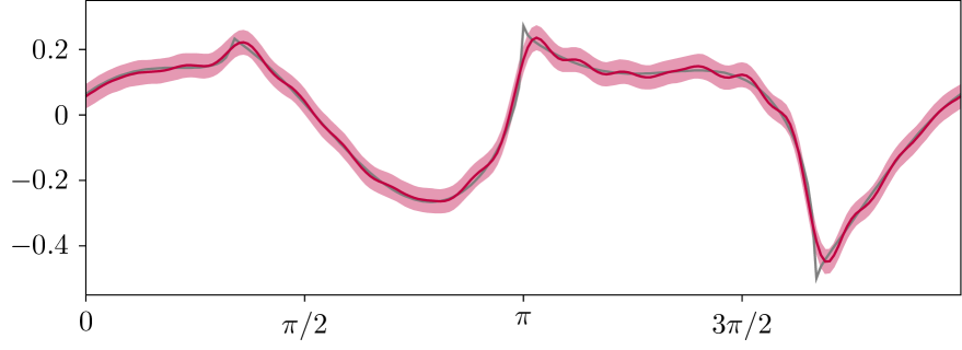
In Figure 2 we repeat the procedure (with new data) but set in the variational class. Now has similar estimates implying that . Generally we observe similar behaviour as before, but the credible regions are narrower. Based on this we conclude that the constant multiplier in the number of inducing variables can play a non-negligible role. In practice the exact choice of is delicate. On the one hand one should choose it as large as the computational resources allow. Increasing beyond a threshold effectively doesn’t help anymore, but this threshold depends on certain hidden properties of the underlying signal. Our theoretical results provide an initial guide for choosing . Then, in practice, if the computational resources allow, one can increase gradually until no significant changes can be observed. This approach combines the asymptotic results with the finite sample size behaviour, making the procedure more robust.
4.1.2 Exponentially decaying eigenvalues – adaptive rescaling
Now consider a series prior with eigenvalues that decay exponentially
| (24) |
where are i.i.d. standard normal random variables and is an orthonormal basis satisfying (11). A prominent example of such eigenvalue structure is the rescaled squared exponential covariance kernel. In this context, we estimate the scaling hyperparameter . If the true Sobolev smoothness of is , then (up to logarithmic factors) the optimal rescaling is of the order and one should take at least inducing variables in the approximation (see Nieman et al. (2022)). We study here the case where is not known, and estimate empirically by maximizing the ELBO over the set
as in (6), where is a lower bound on the true Sobolev smoothness of , which is assumed to satisfy . As before, the inducing variables class (20) is studied for both the empirical and population spectral features, with features.
Corollary 4
Suppose the prior basis in (24) satisfies condition (11) for some . If for some , then the population and empirical spectral features inducing variables variational posteriors corresponding to the prior (24) achieve the (near) minimax contraction rate , i.e.
for an arbitrary sequence tending to infinity.
The proof of the corollary is deferred to Section B.2 in the Appendix.
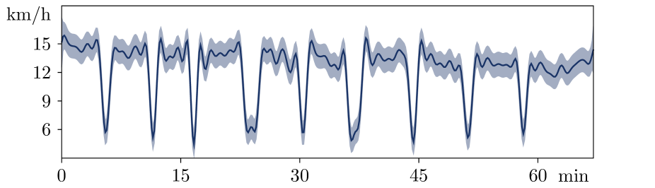
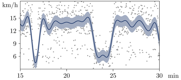
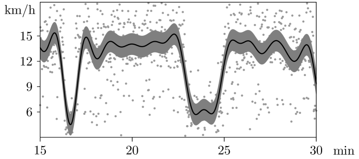
We illustrate the results by applying the procedure to a set of velocity measurements during a run111Code and data are available at https://github.com/dennisnieman/adaptiveVB. A GPS tracker has observed the runner’s coordinates every second during their interval training and the velocity in is estimated from the coordinate shifts. The measurements are smoothed using the squared exponential kernel
| (25) |
Here and are respectively a vertical and a sample path scaling parameter. Since the eigenfunctions in the series expansion of this GP are not known explicitly, we apply the variational approximation with sample spectral features. Both the hyperparameters and the model variance are estimated variationally by maximising the evidence lower bound. Although our theory is developed only for variational estimation of , in practice we also obtain reasonable estimates for the other unknowns, which are comparable to empirical Bayes estimates.
In comparison with the preceding section, here it is not quite clear how should depend on the tuning parameters, since our theory only accounts for the scaling parameter . Therefore we cautiously take large . The sample spectral features were computed using an off-the-shelf eigendecomposition method, which computes the entire decomposition. This is somewhat inefficient, especially since every evaluation of the ELBO requires computation of a new decomposition. Yet already the procedure is almost three times faster than the empirical Bayes procedure. The estimates of are . From the data it becomes clear that the changes in speed are quite abrupt, which is reflected quite well in the variational posterior (see Figure 4). In general, plain stationary GPs are not completely suited to detect jumps and varying local behaviours, and the fit could be improved with a model taking into account change-points.
We compare our variational approximation with the empirical Bayes approach in Figure 5. We estimate the hyperparameters by maximizing the marginal likelihood function , resulting in estimates . By eye, the variational approximation can hardly be distinguished from the empirical Bayes posterior.
4.2 Truncated series priors
As third example, consider a prior of the form
| (26) |
for a uniformly bounded basis (that is, satisfying condition (11) for ). We study a variational procedure for the tuning parameter .
Consider a uniform hyper-prior on the set
In a practical application, the optimisation is faster if the grid is coarser. For example, one might consider the subset of those integers in of the form where . This may worsen the quality of the approximation, even though asymptotic results are unaffected by such a change (as long as a prior is chosen for that satisfies condition (16)).
For fixed , the posterior distribution is a Gaussian process with respective mean and covariance function
where we abbreviate , and denote by the matrix whose -th row is .
Note that the matrix has entries which can be approximated by using the Law of Large Numbers. Thus the posterior distribution is a -dimensional process, and a posteriori the coefficients are nearly diagonal. This motivates the use of the variational class
here viewed as a distribution on the coefficients in the basis . The variational class respects the relationship between the mean and variance of the original posterior. It can also be used to approximate the posterior from a more general Gaussian series prior with coefficients instead of , where the have a decaying structure. For simplicity we restrict ourselves the truncated GP of the form (26).
Denoting , the variational distribution is the maximiser of
over . Next the variational estimator is determined as the maximiser of the function .
Corollary 5
The proof is given in Appendix B.3.
Acknowledgments and Disclosure of Funding
Co-funded by the European Union (ERC, BigBayesUQ, project number: 101041064). Views and opinions expressed are however those of the author(s) only and do not necessarily reflect those of the European Union or the European Research Council. Neither the European Union nor the granting authority can be held responsible for them.
We cordially thank Harry van Zanten for the fruitful discussions in the early stages of writing this paper.
Appendix A Proof of general contraction rate theorems
In this section we collect the proofs for the contraction rates of the hierarchical, empirical and variational Bayes posteriors. But as a first step we study the asymptotic behaviour of the maximum marginal likelihood estimator (MMLE).
A.1 Asymptotic behavior of the MMLE
We show that with -probability tending to one the maximum marginal likelihood estimator defined in (17) belongs to the set of good hyperparameters defined in (15), where the corresponding posteriors nearly attain the oracle rate . The lemma below is an adaptation of Theorem 2.1 of Rousseau and Szabo (2017) to the random design regression model. A major difference is that we consider general basis functions satisfying certain boundedness and tail assumptions, see below. Since the proof consists several new technical arguments compared to Rousseau and Szabo (2017), we provide the whole proof for completeness and easier readability.
Proof We bound the evidence from below using Lemma 10 in Ghosal and van der Vaart (2007). In their notation with and , for as in (9), it follows that
with , where the last equation follows from Lemma 2.7 in Ghosal and van der Vaart (2017). Consequently, we obtain for any
| (28) |
This holds in particular for that minimises , that is,
| (29) |
where for convenience we define . Since is defined as the maximiser of the integral, it follows that
| (30) |
The proof of (27) is completed by showing that
| (31) |
Indeed, together with the preceding display this implies that with probability tending to one the evidence is maximised at some . The proof of (31) is done via a prior mass and testing argument.
Comparison of norms
For in condition (11) let and denote the matrix with entries . Then by Rudelson (1999),
where is the -dimensional identity matrix, and is the Euclidean operator norm. So the event
| (32) |
has -probability going to 1. If and , then
More generally, if , then the truncated series satisfies on the event
| (33) |
Remaining prior mass and entropy
For arbitrary we construct a set such that
| (34) |
and
| (35) |
where denotes the minimal number of -balls of radius required to cover the set .
We follow the construction in Theorem 2.1 in van der Vaart and van Zanten (2008a). Let us start by introducing the concentration function
| (36) |
where is the reproducing kernel Hilbert space of the prior kernel . By Lemma 5.3 in van der Vaart and van Zanten (2008b) and by definition of , it follows that
Together with assumption (14) we obtain the concentration inequality
| (37) |
Define where denotes the standard normal CDF and let
where and denote the unit balls of and , respectively. By the inequality from Borell (1975) and (37) (and ) it follows that
Furthermore, the argument in the proof of Theorem 2.1 in van der Vaart and van Zanten (2008a) shows that (37) implies
which is (35).
Testing
Given any hyperparameter and constant small enough we construct a test for versus the set
From the entropy bound (35) we obtain a cover of this set by at most balls of the form . By doubling the radii of the balls, we may move the centers inside the set , so that in particular and for every .
Consider in the event from (32) and consider both in and in one of the balls in the aforementioned cover. For we have , so we obtain for and ,
| (38) |
It follows that
This implies in particular that . By Lemma 8 it follows that for every there exists a test such that
and (from the preceding display)
For , it follows that the test satisfies, for any ,
| (39) |
and
| (40) |
Completion of the argument
We are now ready to prove (31). Using the tests defined above, note that
| (42) | ||||
| (43) | ||||
| (44) |
We showed earlier that has probability tending to zero. By (39) the sum of type I errors in (42) has upper bound
This term vanishes by the assumption on the size of . Similarly (40) implies that the sum in (43) is bounded from above by
and so the full term (43) vanishes. Finally, using (41), the term in (44) is bounded from above by
which also vanishes.
A.2 Contraction rate for the empirical Bayes posterior
Let us recall the definition of the empirical Bayes posterior given in (18), which is attained by plugging in the MMLE to the posterior distribution. This empirical approach is often used in practice as a natural and computationally more convenient data-driven tuning instead of the hierarchical Bayes method. The theorem below is the adaptation of Theorem 2.2 of Rousseau and Szabo (2017) to our setting. Similarly to Lemma 6, several technical issues had to be overcome when relating the empirical and standard -norms, hence we provide the main steps of the proof below.
Theorem 7
Under the conditions of Lemma 6, there exists large enough such that
Proof [Proof of Theorem 7] We slightly adapt the prior mass and testing argument from the proof of Lemma 6 to accomodate . For any such we define
where . Here the concentration inequality is , and the argument in the proof of Lemma 6 gives
| (45) |
and
| (46) |
For we construct a test for versus the set
Here we note that any with satisfies on , for and ,
Covering the set with at most balls and taking sufficiently large, it follows that there exists a test with
| (47) |
and
| (48) |
Let us define the test . Note that by (27) and (30), the event
| (49) |
has probability tending to 1 (where as in the proof of Lemma 6). Then, by Bayes’ rule,
| (50) |
The type I error can be bounded using (47) as
which vanishes due to the assumption on . To bound the remainder in (50), in view of (48), (46), and condition (13) we obtain
Hence, the full last term in (50) is bounded by for large enough, concluding the proof of our statement.
A.3 Proof of Theorem 1
The proof extends the results on the empirical Bayes posterior to the hierarchical Bayes method, see for instance Szabó et al. (2013); Knapik et al. (2016); Rousseau and Szabo (2017) for similar derivations. One of the key difference is the explicit exponential upper bound for the posterior contraction, needed to obtain frequentist guarantees for the variational approximation.
Let us split the probability to the cases when and , i.e.
| (51) |
We first bound the top term. By (29), with the particular such that , we have
| (52) |
Likewise, (31) gives
| (53) |
On the intersection of the two events we have
for large enough, where we used Bayes’ rule and the assumption (16).
A.4 Proof of Theorem 2
Appendix B Proofs for the examples
In this section we provide the proofs for the contraction rates for the specific choices of Gaussian process priors and variational approaches using Theorem 2. But before that we introduce some notations.
The reproducing kernel Hilbert space associated to a GP with series expansion (10) is the subspace of consisting of those functions such that
This quantity is the squared RKHS norm .
In the examples below we compute by solving the inequality , where is the concentration function defined in (36). By Lemma 5.3 in van der Vaart and van Zanten (2008b), it follows that (for )
which implies is an upper bound for (as defined in (9)). Similarly, if solves , it is a lower bound for .
In each corollary we verify the conditions of Theorem 2. First we show the tail condition (12) on the signal holds with for sufficiently smooth signals. Note that for the Cauchy-Schwarz inequality gives
Hence this lower bound for will always be assumed.
B.1 Proof of Corollary 3
We verify the remaining conditions of Theorem 2. Here the smoothness parameter is selected empirically. First note that in view of Corollary 4.3 in Dunker et al. (1998) there exists a constant independent of such that for small enough
| (58) |
Recall that we have assumed so . Letting , note that
With it follows that for all sufficiently small
so the concentration function can be bounded for as
which implies . The that maximises has at most distance to , so it satisfies
We take to be this particular . Consequently,
Since it follows that the contraction rate is
as soon as we verify the remaining conditions of Theorem 2 for the current choice of prior and variational scheme.
The lower bound in (58) also gives for a small multiple of , and it follows that .
Now let us consider condition (13). We use a technique similar to the proof of Lemma 7 in Randrianarisoa and Szabo (2023). We have already bounded hence . Since and it follows that for not too fast, . For such a , by the assumptions on , there exists such that (for large enough)
Therefore, by the Chernoff bound with , since , it holds that for some
Using it follows that for some ,
Optimising over , it follows that the term in the exponent is of the order
where since . Hence (13) is satisfied for as given.
Condition (16) is satisfied because the hyper-prior is uniform on a set of cardinality .
It remains to verify the condition (19) on the KL-divergence. Recall that is an upper bound for computed by solving the concentration inequality . Consider a which is at most distance away from . It was already shown above that . The concentration inequality implies that there exists such that and . Combining this with Lemma 3 in Nieman et al. (2022) it follows that
Hence it suffices to show that
| (60) |
and
| (61) |
In view of Lemma 4 and 5 of Nieman et al. (2022) the bounds (60) and (61) are satisfied for the variational classes studied here with polynomially decaying prior eigenvalues and number of spectral features exceeding . However, these bounds were shown under the assumption that the eigenfunctions of the prior are bounded by a constant. This means that for the population spectral features we have to slightly adapt the argument, since the assumption on the eigenfunctions is weakened to (11) in the present paper. For the empirical features the result does not rely on this bound and is hereby proved.
For the population spectral features, Hoeffding’s lemma gives
| (62) |
hence by a union bound,
Correspondingly, for , the proof of Lemma 5 in Nieman et al. (2022) gives
and
Taking , the element of closest to , we recall that . For and it follows that (60) and (61) are satisfied. Hence for the population spectral features the condition on the KL-divergence in Theorem 2 is satisfied which gives
thereby concluding the proof.
B.2 Proof of Corollary 4
We first determine an upper bound for . In view of Lemma 9 and 10 given below, for , the concentration function (36) is bounded from above by
for some universal constant . If then
Taking for sufficiently large constant , in view of , we have for any
while for with large enough, it follows that
Hence the concentration function inequality is solved by equal to the maximum of the three preceding lower bounds, which gives
The expression on the right is minimised for
| (63) |
(over the set we obtain this number up to at most a factor ) hence
As before any solution to the reverse concentration inequality gives a lower bound for . In this case Lemma 10 shows that equal to a small multiple of works for any . It follows that .
To verify condition (13), we show first that the exponentially decaying coefficients are bounded up to a constant by the polynomially decaying coefficients from the other example. A linear approximation of the function at gives
for and . Recalling that and where , it follows that the term in the exponent is bounded from below by , for some . Therefore the term is uniformly bounded away from 0 for , , and the preceding display implies that there exists a positive constant such that
for all , and . Hence the tail bound (13) follows from its counterpart for polynomially decaying eigenvalues in the proof of Corollary 3.
Lemma 10 also shows that there exists such that for arbitrary fixed and ,
verifying condition (14) for .
Condition (16) is also satisfied because the hyper-prior is uniform on a set with cardinality of the order .
Again the proof is concluded by bounding the KL-divergence between the variational posterior and the true posterior. In this case we note that for
we have
Since is decreasing on it follows that
Consequently, both the trace term and operator norm term decay faster than any power of , hence Lemma 3 in Nieman et al. (2022) gives
We slightly enlarge to . Then all conditions in Theorem 2 are (still) satisfied and , concluding the proof.
B.3 Proof of Corollary 5
We apply Theorem 2. In view of Lemma 11 and 12, for large enough
solves the concentration inequality for large enough. This provides an upper bound for the oracle rate . The value of that minimises the upper bound is of the order and hence
The lower bound on the small ball exponent in Lemma 12 gives a lower bound for . Solving it follows that , hence .
Next, for
so condition (12) is satisfied for . Since for any , the right-hand side of (13) is always zero, so this condition is trivially satisfied.
It remains to bound the KL-divergence. For as above, take the distribution , where a diagonal matrix with entries and . For convenience let us write and . Using the exact form of it can be seen that
| (64) |
In expectation the trace term cancels out so we have to bound the expectation of the logarithmic term and the quadratic form in this display.
Akin to (62), by Hoeffding’s inequality, note that
By increasing the right hand side is bounded by an arbitrary negative power of . Let us define the complementary event
Now by Gershgorin’s Circle Theorem, on the event , any eigenvalue of the matrix satisfies for some between and
For the optimal of the order , it follows from the assumption that the upper bound is and
To bound the quadratic term in (64) we need a slightly tighter bound on the largest eigenvalue of the difference
for the same optimal value of . We bound the largest eigenvalue of this difference by the Bernstein inequality for matrices. By e.g. Theorem 1.6 in Tropp (2012),
| (65) |
where is a deterministic upper bound for the largest absolute eigenvalue of the matrix and
as follows from the inequality
The above display also implies that we can let . For it follows that the term is dominated by the upper bound for , so for large enough
By increasing the constant , the probability in (65) is bounded by an arbitrary negative power of , hence the complementary event
has probability tending to .
We are finally ready to bound the term
The Hoeffding bound shows that on the event the eigenvalues of are bounded by . Consequently, combined with the Bernstein bound for , we obtain
and it follows that
| (66) |
The term on the right can be expanded as
For the terms in the sum equal . For , we note that by the Cauchy-Schwarz inequality,
so is bounded due to the assumptions on its Sobolev smoothness and the uniform bound on . This implies that for
Altogether we obtain
so recalling (66) it follows that
completing the proof of the corollary.
Appendix C Technical lemmas
The following lemma is a standard testing result using empirical -norm. Below we provide a version with explicit constants and for completeness provide a proof as well.
Lemma 8
For any , there exists a sequence of tests satisfying
Proof By the Chernoff bound, using that under ,
the likelihood ratio test has type 1 error
For such that , note that
so, similarly, the type 2 error of this test is
Lemma 9
Let be the RKHS of the prior in (24). If for some and , then for all and any sufficiently small ,
Proof For sufficiently small, let be a positive integer such that
and define the function . Note that for this and ,
By convexity of the function for positive , it follows that
Then we obtain
so the statement of the lemma follows.
Lemma 10
Let be the prior in (24). There exists a constant such that for all and small enough ,
Proof For the upper bound, we follow the proof of Lemma 11.47 in Ghosal and van der Vaart (2017). For all sufficiently small , let be such that
We note that such exists, since the function is monotone decreasing for and the largest solution of for tends to infinity. Hence and for the function will take a larger value than . Furthermore, note that , so
Note that as , and using the Central Limit Theorem. Regarding the remaining part of the sum, by Markov’s inequality,
where the identity for the integral follows by repeated partial integration. Combining all of the above and realising that as , it follows that
To bound the small ball probability from below, fix and (for sufficiently small) take to be the largest positive integer satisfying the inequality . The Chernoff bound for the distribution yields
so, using again ,
Lemma 11
Let be the prior defined in (26) and its RKHS. Then for any , and ,
Proof
The argument is as in the proof of Lemma 9. Taking we note that and so the infimum is bounded by .
Lemma 12
Let be the RKHS of the prior (26). There exist constants and such that for all and ,
Proof For a chi-squared random variable with degrees of freedom and , the Chernoff bound gives
On the other hand, note first that by Stirling’s approximation for the Gamma function,
so by partial integration,
The result follows by realising that the term dominates for small .
References
- Alquier and Ridgway (2020) Pierre Alquier and James Ridgway. Concentration of tempered posteriors and of their variational distributions. The Annals of Statistics, 48(3):1475–1497, 2020.
- Arbel et al. (2013) Julyan Arbel, Ghislaine Gayraud, and Judith Rousseau. Bayesian Optimal Adaptive Estimation Using a Sieve Prior. Scandinavian Journal of Statistics, 40(3):549–570, 2013.
- Borell (1975) Christer Borell. The Brunn-Minkowski Inequality in Gauss Space. Inventiones mathematicae, 30:207–216, 1975.
- Burt et al. (2020) David R. Burt, Carl Edward Rasmussen, and Mark van der Wilk. Convergence of Sparse Variational Inference in Gaussian Processes Regression. Journal of Machine Learning Research, 21(131):1–63, 2020.
- Chérief-Abdellatif (2019) Badr-Eddine Chérief-Abdellatif. Consistency of ELBO maximization for model selection. In Symposium on Advances in Approximate Bayesian Inference, pages 11–31. PMLR, 2019.
- Chérief-Abdellatif and Alquier (2018) Badr-Eddine Chérief-Abdellatif and Pierre Alquier. Consistency of variational Bayes inference for estimation and model selection in mixtures. Electronic Journal of Statistics, 12:2995–3035, 2018.
- de Jonge and van Zanten (2010) R. de Jonge and J.H. van Zanten. Adaptive nonparametric Bayesian inference using location-scale mixture priors. The Annals of Statistics, 38(6):3300–3320, 2010.
- Donnet et al. (2018) Sophie Donnet, Vincent Rivoirard, Judith Rousseau, and Catia Scricciolo. Posterior concentration rates for empirical Bayes procedures with applications to Dirichlet process mixtures. Bernoulli, 24(1):231–256, 2018.
- Dunker et al. (1998) T. Dunker, M.A. Lifshits, and W. Linde. Small deviation probabilities of sums of independent random variables. In High dimensional probability, pages 59–74. Springer, 1998.
- Gardner et al. (2018) Jacob R. Gardner, Geoff Pleiss, David Bindel, Kilian Q. Weinberger, and Andrew Gordon Wilson. GPyTorch: Blackbox Matrix-Matrix Gaussian Process Inference with GPU Acceleration. In Advances in Neural Information Processing Systems, volume 31, pages 7576–7586, 2018.
- Ghosal and van der Vaart (2007) Subhashis Ghosal and Aad van der Vaart. Convergence rates of posterior distributions for noniid observations. The Annals of Statistics, 35(1):192–223, 2007.
- Ghosal and van der Vaart (2017) Subhashis Ghosal and Aad van der Vaart. Fundamentals of nonparametric Bayesian inference, volume 44. Cambridge University Press, 2017.
- Hensman et al. (2013) James Hensman, Nicolò Fusi, and Neil D. Lawrence. Gaussian processes for big data. arXiv preprint, 2013.
- Knapik et al. (2016) Bartek T Knapik, Botond T Szabó, Aad W Van Der Vaart, and J Harry van Zanten. Bayes procedures for adaptive inference in inverse problems for the white noise model. Probability Theory and Related Fields, 164(3):771–813, 2016.
- Nieman et al. (2022) Dennis Nieman, Botond Szabo, and Harry van Zanten. Contraction rates for sparse variational approximations in gaussian process regression. Journal of Machine Learning Research, 23(205):1–26, 2022.
- Nieman et al. (2023) Dennis Nieman, Botond Szabo, and Harry van Zanten. Uncertainty quantification for sparse spectral variational approximations in Gaussian process regression. Electronic Journal of Statistics, 17:2250––2288, 2023.
- Ohn and Lin (2024) Ilsang Ohn and Lizhen Lin. Adaptive variational Bayes: Optimality, computation and applications. The Annals of Statistics, 52(1):335–363, 2024.
- Randrianarisoa and Szabo (2023) Thibault Randrianarisoa and Botond Szabo. Variational Gaussian processes for linear inverse problems. Advances in Neural Information Processing Systems, 36:28960–28972, 2023.
- Ray and Szabó (2022) Kolyan Ray and Botond Szabó. Variational Bayes for High-Dimensional Linear Regression With Sparse Priors. Journal of the American Statistical Association, 117(539):1270–1281, 2022.
- Rousseau and Szabo (2017) Judith Rousseau and Botond Szabo. Asymptotic behaviour of the empirical Bayes posteriors associated to maximum marginal likelihood estimator. The Annals of Statistics, 45(2):833–865, 2017.
- Rudelson (1999) Mark Rudelson. Random vectors in the isotropic position. Journal of Functional Analysis, 164:60–72, 1999.
- Stankewitz and Szabó (2024) Bernhard Stankewitz and Botond Szabó. Contraction rates for conjugate gradient and Lanczos approximate posteriors in Gaussian process regression. arXiv preprint, 2024.
- Szabó et al. (2013) B.T. Szabó, A.W. van der Vaart, and J.H. van Zanten. Empirical Bayes scaling of Gaussian priors in the white noise model. Electronic Journal of Statistics, 7:991–1018, 2013.
- Titsias (2009a) Michalis Titsias. Variational model selection for sparse Gaussian process regression. Report, University of Manchester, UK, 2009a.
- Titsias (2009b) Michalis K. Titsias. Variational Learning of Inducing Variables in Sparse Gaussian Processes. In Proceedings of the 12th International Conference on Artificial Intelligence and Statistics, pages 567–574. PMLR, 2009b.
- Tropp (2012) Joel A. Tropp. User-friendly tail bounds for sums of random matrices. Foundations of computational mathematics, 12(4):389–434, 2012.
- van der Vaart and van Zanten (2008a) A.W. van der Vaart and J.H. van Zanten. Rates of contraction of posterior distributions based on Gaussian process priors. The Annals of Statistics, 36(3):1435–1463, 2008a.
- van der Vaart and van Zanten (2008b) A.W. van der Vaart and J.H. van Zanten. Reproducing kernel Hilbert spaces of Gaussian priors. Pushing the Limits of Contemporary Statistics: Contributions in Honor of Jayanta K. Ghosh, pages 200–222, 2008b.
- Wenger et al. (2022) Jonathan Wenger, Geoff Pleiss, Marvin Pförtner, Philipp Hennig, and John P. Cunningham. Posterior and Computational Uncertainty in Gaussian Processes. Advances in Neural Information Processing Systems, 35:10876–10890, 2022.
- Yang et al. (2020) Yun Yang, Debdeep Pati, and Anirban Bhattacharya. -variational inference with statistical guarantees. The Annals of Statistics, 48(2):886–905, 2020.
- Zhang and Gao (2020a) Fengshuo Zhang and Chao Gao. Convergence rates of variational posterior distributions. The Annals of Statistics, 48(4):2180–2207, 2020a.
- Zhang and Gao (2020b) Fengshuo Zhang and Chao Gao. Convergence rates of empirical Bayes posterior distributions: a variational perspective. arXiv preprint, 2020b.