The spinning self-force EFT: 1SF waveform recursion relation and Compton scattering

Abstract

Building on recent approaches, we develop an effective field theory for the interaction of spinning particles modeling Kerr black holes within the gravitational self-force expansion. To incorporate dimensional regularization into this framework, we analyze the Myers-Perry black hole and its particle description, obtaining a novel form of the corresponding linearized stress tensor. We then derive the 1SF self-force effective action up to quadratic order in the spin expansion, identifying a new type of spinning recoil term that arises from integrating out the heavy dynamics. Next, we study the 1SF metric perturbation both from the traditional self-force perspective and through the diagrammatic background field expansion, making contact with the radiative waveform. This leads us to consider a novel recursion relation for the curved space 1SF Compton amplitude, which we study up to one-loop in the wave regime and compare with the flat space one-loop Compton amplitude for Kerr up to quadratic order in spin. Finally, we investigate the 1SF spinning Compton amplitude in the eikonal regime, clarifying how strong-field effects – such as the location of the separatrix – emerge from the resummation of the perturbative weak-field expansion.

I Motivation and introduction

Given the growing sensitivity of the LIGO-Virgo-KAGRA network and the advent of next-generation gravitational wave detectors, there is a pressing call for high-precision theoretical waveform templates. However, numerical simulations of compact binary mergers remain computationally intensive, often obscuring the simplicity of the underlying two-body dynamics.

In an attempt to address this challenge, a host of perturbative approaches have been developed to solve the two-body problem in general relativity (GR). These include the Post-Newtonian (PN) expansion [1, 2], the Post-Minkowskian (PM) theory [3, 4, 5] and the gravitational self-force (GSF) theory [6, 7, 8]. Recently established PM methods rely on the weak-field expansion and apply only to widely separated bodies, while GSF techniques are applicable in the strong gravity regime but are valid where one body is much smaller than the other. It is therefore essential to combine the results from these methods. On one hand, resumming PM observables in the small-mass-ratio regime may shed light on the analytic structure of GSF [9, 10, 11, 12], where most results are numerical. On the other hand, incorporating GSF insights into PM computations could extend weak-field methods to the strong-field regime, i.e. beyond their domain of validity [13, 14, 15].

Motivated by this, a new effective field theory approach for massive particles in GR has been proposed recently in the mass ratio expansion both in the amplitude [16] and worldline [17, 18] formulations. A crucial ingredient in this story is the identification of the metric generated by a spinless point particle with the Schwarzschild black hole solution [19, 20, 21, 22, 23, 24], a fact that has been recently proved non-perturbatively [25, 26]. Interestingly, it was also possible to integrate out the heavy dynamics to obtain a non-local effective action for the light-body dynamics.

Including spin effects is crucial for astrophysical black holes, and treating Kerr black holes as elementary particles [27, 28, 29, 30, 31, 32, 33, 34, 35, 36, 37] has led to remarkable progress in pushing high-precision PM calculations of spinning binary systems [38, 39, 40, 41, 42, 43, 44, 45, 46, 47, 48, 49, 50, 51, 52, 53, 54]. An essential ingredient in this endeavor is the construction of the gravitational Compton amplitude for a massive spinning particle interacting with two gravitons [55, 30, 31, 56, 57, 58, 59, 60, 61, 62, 63, 64, 65, 66, 67, 68, 69, 70, 71], which describes the propagation of gravitons in a Kerr spacetime. This is analogous to the traditional self-force approach [72, 73], where the field at 1SF order is determined – besides the geodesic – by the graviton propagator in the background spacetime.

In this paper, we extend the self-force effective field theory to the case of spinning particles, thereby modeling Kerr black holes using the $\mathcal{N}=2$ supersymmetric worldline formulation developed in Refs. [74, 75, 76] (see also Refs. [77, 78]). In section II, we will discuss the identification of the Myers-Perry black hole [79, 80, 81, 82] with a spinning point particle in $d$ dimensions, inspired by a previous derivation in the Kerr case [28]. This will allow us to use dimensional regularization techniques to set up the spinning self-force EFT in section III, which we will obtain at 1SF order. We will then show how to derive new non-local spinning recoil operators by integrating out the heavy dynamics, extending the previous construction in Refs. [17, 18]. The consequences of the derived 1SF effective action will then be discussed in section IV, first from the traditional self-force perspective and then from the diagrammatic background field method [83, 84, 85, 86, 87, 88, 89, 90, 91]. Finally, in Section V, we consider the relevant 1SF Compton amplitude appearing in the recursion relation, both in the wave and eikonal regimes. We compare it with the gravitational flat space Compton amplitude for Kerr at loop level and demonstrate how resumming the weak-field series allows to make a connection with strong-field effects.

Conventions—Throughout this paper we work in the negative metric signature with $\epsilon_{0123}=1$, $\kappa^{2}=32\pi G_{\mathrm{N}}$ and $c=1$. We adopt the convention $\hat{\delta}^{(d)}(\cdot)=(2\pi)^{d}\delta^{(d)}(\cdot)$ and $\hat{\mathrm{d}}^{d}k=\mathrm{d}^{d}k/(2\pi)^{d}$. We write index symmetrization and anti-symmetrization as $2x^{(\mu}y^{\nu)}=x^{\mu}y^{\nu}+x^{\nu}y^{\mu}$ and $2x^{[\mu}y^{\nu]}=x^{\mu}y^{\nu}-x^{\nu}y^{\mu}$. We denote curved space amplitudes by $\mathcal{M}$ with polarization tensors $\bm{\varepsilon}_{\mu\nu}\!=\!\bm{\varepsilon}_{\mu}\bm{\varepsilon}_{\nu}$, while flat space amplitudes are denoted by $\mathcal{A}$ with polarization tensors $\varepsilon_{\mu\nu}\!=\!\varepsilon_{\mu}\varepsilon_{\nu}$.

II The Myers-Perry metric in a covariant formulation

The Kerr metric in Kerr-Schild form reads

$$\hskip-6.0pt\mathrm{~d} s^{2}=\mathrm{d}t^{2}-\mathrm{d}x^{2}-\mathrm{d}y^{2}-\mathrm{d}z^{2}$$

$$\hskip-19.91684pt\qquad-\frac{2G_{\mathrm{N}}m_{\mathrm{H}}R(a_{\mathrm{H}},\vec{x})^{3}}{R(a_{\mathrm{H}},\vec{x})^{4}+a_{\mathrm{H}}^{2}z^{2}}\Big{[}\mathrm{~d}t+\frac{R(a_{\mathrm{H}},\vec{x})(x\mathrm{~d}x+y\mathrm{~d}y)}{a_{\mathrm{H}}^{2}+R(a_{\mathrm{H}},\vec{x})^{2}}$$

$$\hskip-19.91684pt\qquad\qquad\qquad\qquad+\frac{a_{\mathrm{H}}(y\mathrm{~d}x-x\mathrm{~d}y)}{a_{\mathrm{H}}^{2}+R(a_{\mathrm{H}},\vec{x})^{2}}+\frac{z\mathrm{~d}z}{R(a_{\mathrm{H}},\vec{x})}\Big{]}^{2}\,,$$ (1)

where the spin vector $a_{\mathrm{H}}^{\mu}$ is chosen to be aligned along the $z-$direction, $a_{\mathrm{H}}$ is the (normalized) spin parameter and $R(a_{\mathrm{H}},\vec{x})$ is determined by the constraint

$$x^{2}+y^{2}+z^{2}=R(a_{\mathrm{H}},\vec{x})^{2}+a_{\mathrm{H}}^{2}\left[1-\frac{z^{2}}{R(a_{\mathrm{H}},\vec{x})^{2}}\right]\,.$$ (2)

Unlike the spinless case, there is no proof that this metric is generated by a spinning point particle of mass $m_{\mathrm{H}}$ and spin $a_{\mathrm{H}}$ beyond the leading order in $G_{\mathrm{N}}$ [28], but we will explicitly check the consistency of our calculations at quadratic order in the spin expansion. In a covariant way, we can define a basis of 4 vectors in which the Kerr metric is naturally expanded: the four-velocity $v_{\mathrm{H}}^{\mu}$, the spacetime coordinate $x^{\mu}$, the spin vector $a_{\mathrm{H}}^{\mu}$ and a convenient Levi-Civita dependent vector $L_{\mu}$

$$L_{\mu}=\epsilon_{\mu\nu\alpha\beta}v_{\mathrm{H}}^{\nu}a_{\mathrm{H}}^{\alpha}r^{\beta}\,,$$ (3)

where $r^{\mu}$ is obtained through the action of a spatial projector $P^{\mu\nu}$ on the spacetime coordinate $x^{\mu}$

$$\hskip-8.0ptr^{\mu}=P^{\mu}_{\,\,\,\nu}x^{\nu}=x^{\mu}-(x\cdot v_{\mathrm{H}})v_{\mathrm{H}}^{\mu}\,,\,\,\,P^{\mu\nu}=\eta^{\mu\nu}-v_{\mathrm{H}}^{\mu}v_{\mathrm{H}}^{\nu}\,.$$ (4)

In this basis, after transforming (1) into spherical coordinates $(t,r,\theta,\phi)$, we can write the Kerr metric as

$$\bar{g}_{\mu\nu}=\eta_{\mu\nu}-\frac{2G_{\mathrm{N}}m_{\mathrm{H}}R^{3}l_{\mu}l_{\nu}}{\left(R^{2}+a_{\mathrm{H}}^{2}\right)^{2}\left((x\cdot a_{\mathrm{H}})^{2}+R^{4}\right)}\,,$$ (5)

$$l_{\mu} =v_{\mathrm{H}\mu}\,(a_{\mathrm{H}}^{2}+R^{2})-r_{\mu}\,R-L_{\mu}+a_{\mathrm{H}\mu}\,(x\cdot a_{\mathrm{H}})/R\,,$$ (6)

where the $R$ in (2) is at function of $r$, $a_{\mathrm{H}}$ and $x\cdot a_{\mathrm{H}}$

$$\hskip-10.0ptR(a_{\mathrm{H}},\vec{x})\!=\!\frac{1}{\sqrt{2}}\sqrt{r^{2}-a_{\mathrm{H}}^{2}+\sqrt{4(x\cdot a_{\mathrm{H}})^{2}+\left(r^{2}-a_{\mathrm{H}}^{2}\right)^{2}}}\,.$$ (7)

The Kerr-Schild gauge (5) of the metric is particularly convenient for the PM expansion because it manifestly reduces to the flat one in the limit $G_{\mathrm{N}}\to 0$, while other sets of coordinates (such as Boyer-Lindquist) usually retain their spurious spin dependence in such a limit.

In order to harness effective field theory tools in the mass ratio expansion, we need to employ dimensional regularization. This, necessarily, requires one to define the Myers-Perry metric, which generalizes the Kerr metric to higher dimensions. Building on the original derivation of Ref. [79], we write the $d=2+2n$ Myers-Perry metric with equal spinning parameters $a^{d}_{\mathrm{H}}=a_{i}(d-2)/2$ on the $n$ planes (see appendix E of Ref. [92]) as

$$\hskip-8.0pt\bar{g}^{d}_{\mu\nu}=\eta_{\mu\nu}\!-\!\frac{16\pi G_{\mathrm{N}}m_{\mathrm{H}}}{(d-2)\Omega_{d-2}}\frac{R_{d}^{3}\,\left(R_{d}^{2}+(a^{d}_{\mathrm{H}})^{2}\right)^{-\frac{d}{2}}l^{(d)}_{\mu}l^{(d)}_{\nu}}{\left((x\cdot a^{d}_{\mathrm{H}})^{2}+R_{d}^{4}\right)}\,,\!$$ (8)

$$\hskip-8.0ptl^{(d)}_{\mu}=v_{\mathrm{H}\mu}\,((a^{d}_{\mathrm{H}})^{2}+R_{d}^{2})-r_{\mu}\,R_{d}-\sum_{k=1}^{n}L^{(k)}_{\mu}+a^{d}_{\mathrm{H}\mu}\,(x\cdot a^{d}_{\mathrm{H}})/R_{d}\,,$$

$$\hskip-8.0pt\sum_{k=1}^{n}(x_{k}^{2}+y_{k}^{2})+z^{2}=r^{2}=R_{d}(a^{d}_{\mathrm{H}},\vec{x})^{2}+\left[(a^{d}_{\mathrm{H}})^{2}-\frac{(x\cdot a^{d}_{\mathrm{H}})^{2}}{R_{d}(a^{d}_{\mathrm{H}},\vec{x})^{2}}\right]\,,$$

where $\Omega_{d-2}=2\pi^{\frac{d-1}{2}}/\Gamma\left((d-1)/2\right)$ is the angular measure and we have introduced the coordinate system

$$x_{k} =r_{k}\sin(\theta)\cos(\phi_{k}),\,y_{k}=r_{k}\sin(\theta)\sin(\phi_{k}),\,\,k=1,\dots,n$$

$$\qquad\qquad z=r\cos(\theta)\,,\quad r^{2}=\sum_{k=1}^{n}r^{2}_{k}\,.$$ (9)

Technically, for the covariant form of the metric (8) we are introducing a $d$ dimensional spin vector $(a^{d}_{\mathrm{H}})^{\mu}$ such that the following spin tensor decomposition holds

$$S_{\mu\nu} =\sum_{k=1}^{n}\epsilon^{(k)}_{\mu\nu\alpha\beta}v_{\mathrm{H}}^{\alpha}(a^{d}_{\mathrm{H}})^{\beta}\,,$$ (10)

$$\epsilon^{(k)}_{\mu\nu\alpha\beta} =\ (-1)^{n+1}\epsilon_{\mu\nu\alpha\beta i_{1}j_{2}\dots\widehat{i_{k}j_{k}}\dots i_{n}j_{n}}$$

$$\qquad\qquad\times e^{i_{1}}e^{j_{1}}\cdots\widehat{e^{i_{k}}e^{j_{k}}}\cdots e^{i_{n}}e^{j_{n}}\,,$$

together with $n$ rotation vectors in $d=2+2n$ dimensions

$$L^{(k)}_{\mu} =\epsilon^{(k)}_{\mu\nu\alpha\beta}v_{\mathrm{H}}^{\nu}(a^{d}_{\mathrm{H}})^{\alpha}r^{\beta}\,,\qquad\quad k=1,\dots,n$$ (11)

where $(e_{i_{k}},e_{j_{k}})$ are the unit vectors in the $k$-plane and the hat notation indicates that the corresponding indices and vectors are missing. The definition (11) reduces to (3) for a single plane in $d=4$, and similarly the coordinates (9) reduce to the spherical ones in the same limit.

To make contact with 3-point amplitudes, as discussed in Ref. [28], we can study the 1PM stress tensor for a spinning point particle in $d$ dimensions from the linearized Einstein’s equation. Therefore, with the definition

$$(a^{d}_{\mathrm{H}}*_{k}\partial)_{\mu\nu}=\epsilon^{(k)}_{\mu\nu\alpha\beta}(a^{d}_{\mathrm{H}})^{\alpha}\partial^{\beta}\,,$$ (12)

we find the conjectural expression for the linearized stress tensor of the Myers-Perry black hole (see appendix A)

$$\hskip-6.0pt\hat{T}_{d}^{\mu\nu}(v_{\mathrm{H}},a^{d}_{\mathrm{H}},\partial)=m_{\mathrm{H}}\,\Upsilon\left(\frac{d-3}{2},a^{d}_{\mathrm{H}}\cdot\partial\right)v_{\mathrm{H}}^{\mu}v_{\mathrm{H}}^{\nu}$$

$$+m_{\mathrm{H}}\sum_{k=1}^{n}(a^{d}_{\mathrm{H}}*_{k}\partial)^{(\mu}_{\,\,\,\rho}\Upsilon\left(\frac{d-1}{2},a^{d}_{\mathrm{H}}\cdot\partial\right)v_{\mathrm{H}}^{\nu)}v_{\mathrm{H}}^{\rho}$$

$$+\frac{m_{\mathrm{H}}}{2}\sum_{k,k^{\prime}=1}^{n}\hskip-5.0pt(a^{d}_{\mathrm{H}}*_{k}\partial)^{(\mu}_{\,\,\,\rho}(a^{d}_{\mathrm{H}}*_{k^{\prime}}\partial)^{\nu)}_{\,\,\,\lambda}\Upsilon\left(\frac{d+1}{2},a^{d}_{\mathrm{H}}\cdot\partial\right)v_{\mathrm{H}}^{\rho}v_{\mathrm{H}}^{\lambda}\,,$$

$$\Upsilon(\nu,a^{d}_{\mathrm{H}}\cdot\partial)=\,\,_{0}F_{1}\left(;\nu;-\left(a^{d}_{\mathrm{H}}\cdot\partial/2\right)^{2}\right)\,,$$ (13)

giving the 3-pt amplitude $\mathcal{A}^{d}_{3}=G_{\mathrm{N}}\,\varepsilon_{\mu\nu}(k)\widetilde{T}_{d}^{\mu\nu}(v_{\mathrm{H}},a^{d}_{\mathrm{H}},k)$ with the appropriate factor of $G_{\mathrm{N}}$ included. We stress here that it remains an open question to show that (8) is related to the metric produced by a spinning point particle in $d$ dimensions at all PM orders [81, 82].

III The spinning self-force EFT

Here we use the formalism developed in Refs. [17, 18] (see also Ref. [16]) to describe the classical two-body dynamics in the self-force expansion

$$\mathcal{S}=\mathcal{S}_{\mathrm{GR}}+\mathcal{S}_{\mathrm{L}}+\mathcal{S}_{\mathrm{H}}\,,$$ (14)

where $\mathcal{S}_{\mathrm{GR}}$ is the gravitational (gauge-fixed) Einstein-Hilbert action and $\mathcal{S}_{\mathrm{L}}$ (resp. $\mathcal{S}_{\mathrm{H}}$) stands for the action describing light (resp. heavy) matter degrees of freedom. The gravitational action is defined as

$$\mathcal{S}_{\mathrm{GR}}\! =\!-\frac{1}{16\pi G_{\mathrm{N}}}\int\mathrm{d}^{4}x\sqrt{-g}R+\frac{\lambda^{2}}{32\pi G_{\mathrm{N}}}\int\mathrm{d}^{4}x\sqrt{-\bar{g}}F^{\mu}F_{\mu}\,,$$

$$F_{\mu}=\overline{\nabla}^{\nu}\delta\bm{g}_{\mu\nu}-\frac{1}{2}\overline{\nabla}_{\mu}\delta\bm{g}\,,\quad\delta\bm{g}=\bar{g}^{\mu\nu}\delta\bm{g}_{\mu\nu}\,,$$ (15)

where we have chosen the background field gauge for the perturbation $\lambda\delta\bm{g}_{\mu\nu}=g_{\mu\nu}-\bar{g}_{\mu\nu}$ with $\bar{g}_{\mu\nu}$ being the background metric of a Schwarzschild or a Kerr black hole. In what follows we will first review the self-force EFT for spinless bodies, and then extend the discussion to that of spinning bodies.

Review of the spinless self-force EFT

Let us start by reviewing the spinless case discussed in Refs. [17, 18]. The matter action is defined as

$$\hskip-6.0pt\mathcal{S}_{\mathrm{m}}=-\sum_{i=\mathrm{L},\mathrm{H}}\mathcal{S}_{i}=-\sum_{i=\mathrm{L},\mathrm{H}}m_{i}\int\mathrm{d}\tau\,\frac{1}{2}g_{\mu\nu}\dot{x}_{i}^{\mu}\dot{x}_{i}^{\nu}\,,$$ (16)

where $\tau$ is the proper time, $m_{i}$ is the mass and $x_{i}^{\mu}(\tau)$ is the trajectory of the $i$-th particle obeying the on-shell constraint $\dot{x}_{i}^{2}=1$. As usual, the equation of motion is simply the geodesic equation

$$\ddot{x}_{i}^{\mu}+\Gamma^{\mu}_{~\rho\sigma}(x_{i})\dot{x}_{i}^{\rho}\dot{x}_{i}^{\sigma}=0\,,$$ (17)

where $\Gamma^{\mu}_{~\rho\sigma}$ is the Christoffel connection

$$\Gamma^{\mu}_{~\rho\sigma}=\frac{1}{2}g^{\mu\alpha}(\partial_{\rho}g_{\alpha\sigma}+\partial_{\sigma}g_{\rho\alpha}-\partial_{\alpha}g_{\rho\sigma})\,.$$ (18)

The goal is then to perform the GSF expansion, which is simply an expansion in the small mass ratio $\lambda=m_{\mathrm{L}}/m_{\mathrm{H}}$. At leading order in $\lambda$, we evaluate the action (14) on the Schwarzschild-Tangherlini metric $\bar{g}_{\mu\nu}$ (i.e. taking the limit $a^{d}_{\mathrm{H}}\to 0$ in (8)) and enforce that it is sourced by the heavy particle stress tensor supported on the straight-line trajectory $\bar{x}_{\mathrm{H}}^{\mu}(\tau)=v_{\mathrm{H}}^{\mu}\tau$

$$\begin{split}&\qquad\bar{R}_{\mu\nu}-\frac{1}{2}\bar{g}_{\mu\nu}\bar{R}=8\pi G_{\mathrm{N}}\bar{T}_{\mathrm{H}\mu\nu}\,,\\ &\bar{T}^{\mu\nu}_{\mathrm{H}}=\frac{m_{\mathrm{H}}}{\sqrt{-\bar{g}}}\int\mathrm{d}\tau\delta^{(4)}\left(x-v_{\mathrm{H}}\tau\right)v_{\mathrm{H}}^{\mu}v_{\mathrm{H}}^{\nu}\,,\end{split}$$ (19)

so that the light particle moves in the geodesic trajectory

$$\ddot{\bar{x}}_{\mathrm{L}}^{\mu}+\bar{\Gamma}^{\mu}_{~\rho\sigma}(\bar{x}_{\mathrm{L}})\dot{\bar{x}}_{\mathrm{L}}^{\rho}\dot{\bar{x}}_{\mathrm{L}}^{\sigma}=0\,.$$ (20)

Already at this order, we notice that dimensional regularization is extremely helpful to handle divergent terms involving the metric evaluated on the heavy trajectory $\bar{g}_{\mu\nu}(\bar{x}_{\mathrm{H}})$; these self-energy contributions can be absorbed with a mass counterterm, effectively setting [17, 18]

$$\bar{g}_{\mu\nu}(\bar{x}_{\mathrm{H}})\to\eta_{\mu\nu}\,,\quad\bar{\Gamma}^{\mu}_{~\rho\sigma}(\bar{x}_{\mathrm{H}}),\bar{R}_{\mu\nu\alpha\beta}(\bar{x}_{\mathrm{H}})\to 0\,.$$ (21)

At the first self-force (1SF) order, we perturb the metric and worldline trajectories by corrections [17, 18]

$$x_{i}^{\mu}(\tau) =\bar{x}_{i}^{\mu}(\tau)+\lambda\,\delta x_{i}^{\mu}(\tau)\,,$$

$$g_{\mu\nu}(x) =\bar{g}_{\mu\nu}(x)+\lambda\,\delta\bm{g}_{\mu\nu}(x)\,,$$ (22)

where $\lambda$ is made explicit in the corrections. Using (22), we further expand the metric around the trajectory

$$g_{\mu\nu}(x_{i})=g_{\mu\nu}(\bar{x}_{i})+\lambda\delta x_{i}^{\alpha}\partial_{\alpha}g_{\mu\nu}(\bar{x}_{i})$$

$$\qquad\qquad+\frac{\lambda^{2}}{2}\delta x_{i}^{\alpha}\delta x_{i}^{\beta}\partial_{\alpha}\partial_{\beta}g_{\mu\nu}(\bar{x}_{i})+\mathcal{O}(\lambda^{3})\,.$$ (23)

Substituting (22) and (23) into the combined matter (16) and graviton (15) action (see Ref. [18] and appendix B for more details) we recover the 1SF contribution

$$\mathcal{S}^{\mathrm{1SF}} =\mathcal{S}^{\mathrm{1SF}}_{\mathrm{GR}}+\mathcal{S}^{\mathrm{1SF}}_{\mathrm{L}}+\mathcal{S}^{\mathrm{1SF}}_{\mathrm{H}},$$ (24)

$$\mathcal{S}^{\mathrm{1SF}}_{\mathrm{GR}} =\frac{-\lambda^{2}}{32\pi G_{\mathrm{N}}}\int\mathrm{d}^{4}x\,\sqrt{-\bar{g}}$$

$$\hskip-10.0pt\times\Big{\{}\left(\frac{1}{2}\bar{g}^{\mu\nu}\bar{g}^{\alpha\gamma}\bar{g}^{\beta\delta}-\frac{1}{4}\bar{g}^{\mu\nu}\bar{g}^{\alpha\beta}\bar{g}^{\gamma\delta}\right)\overline{\nabla}_{\mu}\delta\bm{g}_{\alpha\beta}\overline{\nabla}_{\nu}\delta\bm{g}_{\gamma\delta}$$

$$\hskip-10.0pt\quad+\Big{[}\frac{1}{4}\bar{R}(2\bar{g}^{\xi\zeta}\bar{g}^{\xi^{\prime}\zeta^{\prime}}-\bar{g}^{\xi\xi^{\prime}}\bar{g}^{\zeta\zeta^{\prime}})$$

$$\hskip-10.0pt\quad+\bar{R}_{\rho\gamma}(\bar{g}^{\rho\zeta}\bar{g}^{\gamma\zeta^{\prime}}\bar{g}^{\xi\xi^{\prime}}-\bar{g}^{\rho\xi}\bar{g}^{\gamma\zeta}\bar{g}^{\xi^{\prime}\zeta^{\prime}})$$

$$\hskip-10.0pt\qquad\qquad-\bar{R}_{\rho\gamma\sigma\lambda}\bar{g}^{\rho\zeta}\bar{g}^{\sigma\zeta^{\prime}}\bar{g}^{\gamma\xi}\bar{g}^{\lambda\xi^{\prime}}\Big{]}\delta\bm{g}_{\zeta\zeta^{\prime}}\delta\bm{g}_{\xi\xi^{\prime}}\Big{\}}\,,$$

$$\mathcal{S}^{\mathrm{1SF}}_{\mathrm{L}} =-m_{\mathrm{H}}\lambda^{2}\int\mathrm{d}\tau\frac{1}{2}\dot{\bar{x}}_{\mathrm{L}}^{\mu}\dot{\bar{x}}_{\mathrm{L}}^{\nu}\delta\bm{g}_{\mu\nu}\left(\bar{x}_{\mathrm{L}}\right),$$

$$\mathcal{S}^{\mathrm{1SF}}_{\mathrm{H}} =-m_{\mathrm{H}}\lambda^{2}\int\mathrm{d}\tau\Big{\{}\frac{1}{2}\delta\dot{x}_{\mathrm{H}}^{2}-\delta x_{\mathrm{H}}^{\rho}\dot{\bar{x}}_{\mathrm{H}}^{\mu}\dot{\bar{x}}_{\mathrm{H}}^{\nu}\delta\Gamma_{\rho\mu\nu}\left(\bar{x}_{\mathrm{H}}\right)\Big{\}},$$

where we have used the equations of motion at 0SF order, dropped the non-dynamical contributions and defined the variation in the connection

$$\delta\Gamma^{\rho}_{~\mu\nu} =\Gamma^{\rho}_{~\mu\nu}-\bar{\Gamma}^{\rho}_{~\mu\nu}$$

$$=\frac{1}{2}\bar{g}^{\rho\alpha}(\overline{\nabla}_{\mu}\delta\bm{g}_{\nu\alpha}+\overline{\nabla}_{\nu}\delta\bm{g}_{\mu\alpha}-\overline{\nabla}_{\alpha}\delta\bm{g}_{\mu\nu})\,.$$ (25)

It is worth noticing that the distributional nature of the source (i.e. the heavy point particle) does not allow one to set $\bar{R}_{\mu\nu}$ and $\bar{R}$ to zero [16, 17, 18]. Instead, one should consider the Ricci tensor and scalar in the sense of distributions in order to have a consistent theory of interacting point particles [93, 94], where their value is fixed by (19) at the 1SF order. At this point it is important to note that we can formally integrate out the $\delta x_{\mathrm{H}}$ perturbation

$$\delta\ddot{x}^{\mu}_{\mathrm{H}}+\delta\Gamma^{\mu}_{\,\alpha\beta}(\bar{x}_{\mathrm{H}})\dot{\bar{x}}^{\alpha}_{\mathrm{H}}\dot{\bar{x}}^{\beta}_{\mathrm{H}}=0\,,$$

to obtain ($1/\partial_{\tau}$ stands for the integration over $\tau$)

$$\delta x_{\mathrm{H}\mu}=-\frac{1}{\partial_{\tau}^{2}}\Big{[}\delta\Gamma_{\mu\alpha\beta}(\bar{x}_{\mathrm{H}})\dot{\bar{x}}^{\alpha}_{\mathrm{H}}\dot{\bar{x}}^{\beta}_{\mathrm{H}}\Big{]}\,.$$ (26)

Therefore, at the level of the path integral, we obtain an effective 1SF self-force action written only in terms of the graviton and the light particle dynamics

$$\int\mathcal{D}[g]\,\mathcal{D}[x_{\mathrm{L}}]\,\mathcal{D}[x_{\mathrm{H}}]e^{i\mathcal{S}[x_{\mathrm{L}},x_{\mathrm{H}},g]/\hbar}\Big{|}_{\mathrm{1SF}}$$ (27)

$$=\int\mathcal{D}[\delta\bm{g}]\,\mathcal{D}[\delta x_{\mathrm{L}}]\,\mathcal{D}\delta[x_{\mathrm{H}}]\,e^{i(\mathcal{S}^{\mathrm{1SF}}_{\mathrm{GR}}+\mathcal{S}^{\mathrm{1SF}}_{\mathrm{L}}+\mathcal{S}^{\mathrm{1SF}}_{\mathrm{H}})[\delta x_{\mathrm{H}},\delta x_{\mathrm{L}},\delta\bm{g}]/\hbar}$$

$$=\int\mathcal{D}[\delta\bm{g}]\,e^{i(\mathcal{S}^{\mathrm{1SF}}_{\mathrm{GR}}+\mathcal{S}^{\mathrm{1SF}}_{\mathrm{L}}+\mathcal{S}^{\mathrm{1SF}}_{\mathrm{recoil}})[\delta\bm{g}]/\hbar}\,,$$

where we introduced a non-local recoil operator [17, 18]

$$\mathcal{S}^{\mathrm{1SF}}_{\mathrm{recoil}}=-i\hbar\log\left[\int\mathcal{D}[\delta x_{\mathrm{H}}]e^{i\mathcal{S}^{\mathrm{1SF}}_{\mathrm{H}}[\delta x_{\mathrm{L}},\delta x_{\mathrm{H}},\delta\bm{g}]/\hbar}\right]$$ (28)

$$=-\frac{m_{\mathrm{H}}}{2}\int\mathrm{d}\tau\,\left[\dot{\bar{x}}_{\mathrm{H}}^{\alpha}\dot{\bar{x}}_{\mathrm{H}}^{\beta}\delta\Gamma^{\mu}_{~\alpha\beta}(\bar{x}_{\mathrm{H}})\right]\frac{1}{\partial_{\tau}^{2}}\left[\dot{\bar{x}}_{\mathrm{H}}^{\gamma}\dot{\bar{x}}_{\mathrm{H}}^{\delta}\delta\Gamma_{\mu\gamma\delta}(\bar{x}_{\mathrm{H}})\right]\,.$$

In this way, the 1SF effective action can be written as

$$\mathcal{S}^{\mathrm{1SF}}_{\mathrm{eff}}[\delta\bm{g};\{\bar{x}_{\mathrm{L}}\}] \equiv\mathcal{S}^{\mathrm{1SF}}_{\mathrm{GR}}+\mathcal{S}^{\mathrm{1SF}}_{\mathrm{L}}+\mathcal{S}^{\mathrm{1SF}}_{\mathrm{recoil}}\,,$$ (29)

which is a function of a single dynamical field $\delta\bm{g}^{\mu\nu}$ but implicitly depends on the background trajectory $\bar{x}_{\mathrm{L}}^{\mu}$.

The spinning self-force EFT

Having reviewed and understood the self-force expansion for the spinless case, we are now ready to extend this EFT to the spinning case. In doing so, we will restrict our analysis up to quadratic order in spin, taking advantage of the $\mathcal{N}=2$ SUSY worldline model [74, 75, 95]; higher spin orders can be included systematically, for example following Refs. [96, 97, 98, 78]. The matter action is defined as

$$\hskip-8.0pt\mathcal{S}^{\mathrm{spin}}_{\mathrm{m}}=-\sum_{i=\mathrm{L},\mathrm{H}}m_{i}\int\mathrm{d}\tau\Big{\{}\frac{1}{2}g_{\mu\nu}\dot{x}_{i}^{\mu}\dot{x}_{i}^{\nu}+im_{i}\bar{\psi}_{i,a}\frac{D\psi_{i}^{a}}{\mathrm{d}\tau}$$

$$\qquad\qquad\qquad+\frac{m_{i}^{2}}{2}R_{abcd}\bar{\psi}_{i}^{a}\psi_{i}^{b}\bar{\psi}_{i}^{c}\psi_{i}^{d}+\mathcal{O}(S_{i}^{3})\Big{\}}\,,$$ (30)

where Latin indices denote a locally flat spacetime, $\bar{\psi}_{i}$ and $\psi_{i}$ are complex Grassmann variables, and

$$\frac{D\psi_{i}^{a}}{\mathrm{d}\tau}=\dot{\psi}_{i}^{a}+\dot{x}_{i}^{\mu}\omega_{\mu}^{~ab}(x_{i})\psi_{i,b}\,,$$ (31)

with the spin connection $\omega_{\mu}^{~ab}$. Note that we embed fields defined in the local spacetime into the global spacetime using the vielbein $e^{\mu}_{~a}(x)$, e.g. $\psi_{i}^{\mu}(x)=e^{\mu}_{~a}(x)\psi_{i}^{a}$. In this way, the vielbein and the spin tensor are defined as

$$g_{\mu\nu}=e_{\mu}^{a}e_{\nu}^{b}\eta_{ab}\,,\quad S_{i}^{\mu\nu}=-2im_{i}e_{a}^{\mu}e_{b}^{\nu}\bar{\psi}_{i}^{[a}\psi_{i}^{b]}\,,$$ (32)

and the spin connection reads

$$\omega_{\mu}^{~ab}=-\omega_{\mu}^{~ba}=e^{a}_{~\nu}(\partial_{\mu}e^{\nu b}+\Gamma^{\nu}_{~\mu\lambda}e^{\lambda b})\,.$$ (33)

It is straightforward to derive the equations of motion by treating $\bar{\psi}_{i}$ and $\psi_{i}$ as independent variables

$$\dot{\psi}^{a}_{i}+\dot{x}_{i}^{\mu}\omega_{\mu}^{~ab}(x_{i})\psi_{i,b}-im_{i}R_{abcd}(x_{i})\psi_{i}^{b}\bar{\psi}_{i}^{c}\psi_{i}^{d}=0\,,$$ (34)

$$\ddot{x}_{i}^{\mu}+\Gamma^{\mu}_{~\alpha\beta}(x_{i})\dot{x}_{i}^{\alpha}\dot{x}_{i}^{\beta}-\frac{1}{2}R_{\alpha\beta~\nu}^{~~~\mu}(x_{i})\dot{x}_{i}^{\nu}S_{i}^{\alpha\beta}$$ (35)

$$\hskip 22.76219pt\qquad\qquad\qquad+\frac{1}{8}\nabla_{x_{i}}^{\mu}R_{\alpha\beta\rho\lambda}(x_{i})S_{i}^{\alpha\beta}S_{i}^{\rho\lambda}=0\,,$$

where the equation of motion for $\bar{\psi}_{i}$ is given by the conjugate of (34). An important consequence of the mass dependence in the spin tensor (32) is that we expect every power of the spin tensor on the light body (resp. heavy body) to be suppressed (resp. enhanced) compared to the spinless term. Thus, we consider an explicit spin expansion of $\bar{x}_{\mathrm{L}}^{\mu}$ and $\psi^{a}_{\mathrm{L}}$ through quadratic in spin

$$x_{\mathrm{L}}^{\mu}(\tau) =\bar{x}_{\mathrm{L}}^{(0)\mu}(\tau)+\lambda\bar{x}_{\mathrm{L}}^{(1)\mu}(\tau)+\lambda^{2}\bar{x}_{\mathrm{L}}^{(2)\mu}(\tau)+\lambda\delta x_{\mathrm{L}}^{\mu}(\tau)\,,$$

$$\psi^{a}_{\mathrm{L}}(\tau) =\Psi^{(0)a}_{\mathrm{L}}(\tau)+\lambda\Psi^{(1)a}_{\mathrm{L}}(\tau)+\lambda\delta\psi^{a}_{\mathrm{L}}(\tau)\,,$$ (36)

where $\bar{x}_{\mathrm{L}}^{\mu}(\tau)\equiv\bar{x}_{\mathrm{L}}^{(0)\mu}(\tau)+\lambda\bar{x}_{\mathrm{L}}^{(1)\mu}(\tau)+\lambda^{2}\bar{x}_{\mathrm{L}}^{(2)\mu}(\tau)$ and $\Psi^{a}_{\mathrm{L}}(\tau)\equiv\Psi^{(0)a}_{\mathrm{L}}(\tau)+\lambda\Psi^{(1)a}_{\mathrm{L}}(\tau)$ satisfy

$$\hskip-5.0pt\dot{\Psi}^{a}_{\mathrm{L}}+\dot{\bar{x}}_{\mathrm{L}}^{\mu}\bar{\omega}_{\mu}^{~ab}(\bar{x}_{\mathrm{L}})\Psi_{\mathrm{L},b}-im_{\mathrm{L}}\bar{R}_{abcd}(\bar{x}_{\mathrm{L}})\Psi_{\mathrm{L}}^{b}\bar{\Psi}_{\mathrm{L}}^{c}\Psi_{\mathrm{L}}^{d}=0\,,$$

$$\hskip-5.0pt\ddot{\bar{x}}_{\mathrm{L}}^{\mu}+\bar{\Gamma}^{\mu}_{~\alpha\beta}(\bar{x}_{\mathrm{L}})\dot{\bar{x}}_{\mathrm{L}}^{\alpha}\dot{\bar{x}}_{\mathrm{L}}^{\beta}-\frac{1}{2}\bar{R}_{\alpha\beta~\nu}^{~~~\mu}(\bar{x}_{\mathrm{L}})\dot{\bar{x}}_{\mathrm{L}}^{\nu}\bar{S}_{\mathrm{L}}^{\alpha\beta}$$

$$\hskip 11.38109pt\qquad\qquad\qquad+\frac{1}{8}\overline{\nabla}_{\bar{x}_{\mathrm{L}}}^{\mu}\bar{R}_{\alpha\beta\rho\lambda}(\bar{x}_{\mathrm{L}})\bar{S}_{\mathrm{L}}^{\alpha\beta}\bar{S}_{\mathrm{L}}^{\rho\lambda}=0\,,$$ (37)

with the background value of the light particle spin tensor defined as $\bar{S}_{\mathrm{L}}^{\mu\nu}=-2im_{\mathrm{L}}\bar{\Psi}_{\mathrm{L}}^{[\mu}\Psi_{\mathrm{L}}^{\nu]}$. On the other hand, for the heavy particle, we keep all spin contributions

$$x_{\mathrm{H}}^{\mu}(\tau) =\bar{x}_{\mathrm{H}}^{\mu}(\tau)+\lambda\delta x_{\mathrm{H}}^{\mu}(\tau)\,,$$

$$\psi^{a}_{\mathrm{H}}(\tau) =\Psi^{a}_{\mathrm{H}}(\tau)+\lambda\delta\psi^{a}_{\mathrm{H}}(\tau)\,,$$ (38)

given that the renormalization of the self-energy corrections (using dimensional regularization to handle divergent terms on the worldline) in (21) already implies

$$\ddot{\bar{x}}_{\mathrm{H}}^{\mu}=\dot{\Psi}^{a}_{\mathrm{H}}=0\,.$$ (39)

Notice that by expanding the $d$-dimensional Myers-Perry metric (8) around $d=4-2\epsilon$ we have effectively dropped the contributions from $L_{\mu}^{(k)}$ with $k>1$, consistently with the fact that our spinning particle lives in a four-dimensional spacetime. Therefore, we obtain the effective action at 0SF order

$$\mathcal{S}^{\mathrm{spin},\mathrm{0SF}}_{\mathrm{m}} =-m_{\mathrm{H}}\lambda\int\mathrm{d}\tau\,\frac{1}{2}\bar{g}_{\mu\nu}(\bar{x}_{\mathrm{L}}^{(0)})\dot{x}_{\mathrm{L}}^{(0)\mu}\dot{x}_{\mathrm{L}}^{(0)\nu}$$ (40)

$$-m_{\mathrm{H}}\int\mathrm{d}\tau\,\left[\frac{1}{2}\eta_{\mu\nu}\dot{\bar{x}}_{\mathrm{H}}^{\mu}\dot{\bar{x}}_{\mathrm{H}}^{\nu}+im_{\mathrm{H}}\bar{\Psi}_{\mathrm{H}a}\dot{\Psi}_{\mathrm{H}}^{a}\right]\,,$$

where the 0SF trajectory for the heavy and light body is

$$\bar{x}_{\mathrm{H}}^{\mu}(\tau)=v_{\mathrm{H}}^{\mu}\tau\,,\qquad\psi^{a}_{\mathrm{H}}(\tau)=\Psi^{a}_{\mathrm{H}}\,,$$ (41)

$$\,\ddot{\bar{x}}_{\mathrm{L}}^{(0)\mu}+\bar{\Gamma}^{\mu}_{~\alpha\beta}(\bar{x}_{\mathrm{L}}^{(0)})\dot{\bar{x}}_{\mathrm{L}}^{(0)\alpha}\dot{\bar{x}}_{\mathrm{L}}^{(0)\beta}=0\,,$$

together with $\bar{S}_{\mathrm{H}}^{\mu\nu}=-2im_{\mathrm{H}}\bar{\Psi}_{\mathrm{H}}^{[\mu}\Psi_{\mathrm{H}}^{\nu]}$. As stressed earlier, it is crucial to note that the mass scaling (32) forces us to treat the light body as spinless at 0SF order, while the heavy particle carries a tower of spinning contributions.

Moving on to the 1SF order, both the spinless and linear in spin contributions of $\bar{x}_{\mathrm{L}}^{\mu}$ will be relevant, as well as the leading contribution of $\Psi^{a}_{\mathrm{L}}$ and $\bar{\Psi}^{a}_{\mathrm{L}}$. To perform the GSF expansion of the action, we expand the spin connection and Riemann tensor around their background value

$$\begin{split}&\omega_{\mu}^{~ab}(x)=\bar{\omega}_{\mu}^{~ab}(x)+\sum_{n=1}^{\infty}\lambda^{n}\delta\omega^{(n)ab}_{\mu}(x)\,,\\ &R_{abcd}(x)=\bar{R}_{abcd}(x)+\sum_{n=1}^{\infty}\lambda^{n}\delta R^{(n)}_{abcd}(x)\;,\end{split}$$ (42)

where the variations admit an expansion in $\delta\bm{g}_{\mu\nu}$ with $(n)$ denoting the corresponding order. Combining the linear contribution in $\delta\bm{g}_{\mu\nu}$ from the matter (30) and graviton (15) actions, together with the following identities (see appendix B for details)

$$m_{\mathrm{H}}\int\mathrm{d}\tau\,\dot{\bar{x}}_{\mathrm{H}}^{\mu}\bar{\Psi}_{\mathrm{H}}^{a}\delta\omega^{(1)}_{\mu ab}(\bar{x}_{\mathrm{H}})\Psi_{\mathrm{H}}^{b}$$ (43)

$$=-\frac{i}{2}\int\mathrm{d}^{4}x\int\mathrm{d}\tau\,\delta\bm{g}_{\mu\nu}v_{\mathrm{H}}^{(\mu}(\bar{S}_{\mathrm{H}}\cdot\partial_{x})^{\nu)}\delta^{4}\left(x-v_{\mathrm{H}}\tau\right)\,,$$

$$m_{\mathrm{H}}^{2}\int\mathrm{d}\tau\,\delta R^{(1)}_{abcd}(\bar{x}_{\mathrm{H}})\bar{\Psi}_{\mathrm{H}}^{a}\Psi_{\mathrm{H}}^{b}\bar{\Psi}_{\mathrm{H}}^{c}\Psi_{\mathrm{H}}^{d}$$ (44)

$$=\frac{1}{2}\int\mathrm{d}^{4}x\int\mathrm{d}\tau\,\delta\bm{g}_{\mu\nu}(\bar{S}_{\mathrm{H}}\cdot\partial_{x})^{(\mu}(\bar{S}_{\mathrm{H}}\cdot\partial_{x})^{\nu)}\delta^{4}\left(x-v_{\mathrm{H}}\tau\right)\,,$$

we obtain Einstein’s equation (19) with

$$\bar{T}^{\mu\nu}_{\mathrm{H},{\mathrm{spin}}}=\frac{m_{\mathrm{H}}}{\sqrt{-\bar{g}}}\int\mathrm{d}\tau\Big{[}v_{\mathrm{H}}^{\mu}v_{\mathrm{H}}^{\nu}+v_{\mathrm{H}}^{(\mu}(\bar{S}_{\mathrm{H}}\cdot\partial_{x})^{\nu)}$$ (45)

$$\qquad\qquad\quad+\frac{1}{2}(\bar{S}_{\mathrm{H}}\cdot\partial_{x})^{(\mu}(\bar{S}_{\mathrm{H}}\cdot\partial_{x})^{\nu)}\Big{]}\delta^{4}\left(x-v_{\mathrm{H}}\tau\right)\,.$$

The spinning extension of the 1SF effective action in (29) takes the form (see appendix B for details)

$$\mathcal{S}^{\mathrm{spin},\mathrm{1SF}}=\mathcal{S}^{\mathrm{1SF}}_{\mathrm{GR}}+\mathcal{S}^{\mathrm{spin},\mathrm{1SF}}_{\mathrm{L}}+\mathcal{S}^{\mathrm{spin},\mathrm{1SF}}_{\mathrm{H}}\,,$$ (46)

$$\mathcal{S}^{\mathrm{spin},\mathrm{1SF}}_{\mathrm{L}}=-m_{\mathrm{H}}\lambda^{2}\int\mathrm{d}\tau\Big{\{}\frac{1}{2}\dot{\bar{x}}_{\mathrm{L}}^{(0)\mu}\dot{\bar{x}}_{\mathrm{L}}^{(0)\nu}\delta\bm{g}_{\mu\nu}(\bar{x}_{\mathrm{L}}^{(0)})$$

$$\qquad+\frac{1}{2}\dot{\bar{x}}_{\mathrm{L}}^{(0)\mu}\dot{\bar{x}}_{\mathrm{L}}^{(0)\nu}\bar{x}_{\mathrm{L}}^{(1)\rho}\partial_{\rho}g_{\mu\nu}(\bar{x}_{\mathrm{L}}^{(0)})+\dot{\bar{x}}_{\mathrm{L}}^{(1)\mu}\dot{\bar{x}}_{\mathrm{L}}^{(0)\nu}\bar{g}_{\mu\nu}(\bar{x}_{\mathrm{L}}^{(0)})$$

$$\qquad+im_{\mathrm{H}}\bar{\Psi}^{(0)}_{\mathrm{L}a}\dot{\Psi}_{\mathrm{L}}^{(0)a}+im_{\mathrm{H}}\dot{\bar{x}}_{\mathrm{L}}^{(0)\mu}\bar{\Psi}^{(0)a}_{\mathrm{L}}\omega_{\mu ab}(\bar{x}_{\mathrm{L}}^{(0)})\Psi^{(0)b}_{\mathrm{L}}\Big{\}},$$

$$\mathcal{S}^{\mathrm{spin},\mathrm{1SF}}_{\mathrm{H}}=-m_{\mathrm{H}}\lambda^{2}\int\mathrm{d}\tau\Big{\{}\frac{1}{2}\delta\dot{x}_{\mathrm{H}}^{2}-\delta x_{\mathrm{H}}^{\rho}\dot{\bar{x}}_{\mathrm{H}}^{\mu}\dot{\bar{x}}_{\mathrm{H}}^{\nu}\delta\Gamma_{\rho\mu\nu}\left(\bar{x}_{\mathrm{H}}\right)$$

$$\qquad+im_{\mathrm{H}}\delta\bar{\psi}_{\mathrm{H}a}\delta\dot{\psi}^{a}_{\mathrm{H}}+im_{\mathrm{H}}\delta\dot{x}_{\mathrm{H}}^{\mu}\bar{\Psi}_{\mathrm{H}a}\delta\omega_{\mu}^{(1)ab}(\bar{x}_{\mathrm{H}})\Psi_{\mathrm{H}b}$$

$$\qquad+im_{\mathrm{H}}\dot{\bar{x}}_{\mathrm{H}}^{\mu}\delta x_{\mathrm{H}}^{\alpha}\bar{\Psi}_{\mathrm{H}a}\partial_{\alpha}\delta\omega_{\mu}^{(1)ab}(\bar{x}_{\mathrm{H}})\Psi_{\mathrm{H}b}$$

$$\qquad+im_{\mathrm{H}}\dot{\bar{x}}_{\mathrm{H}}^{\mu}\left(\delta\bar{\psi}_{\mathrm{H}a}\Psi_{\mathrm{H}b}+\bar{\Psi}_{\mathrm{H}a}\delta\psi_{\mathrm{H}b}\right)\delta\omega_{\mu}^{(1)ab}(\bar{x}_{\mathrm{H}})$$

$$\qquad+m_{\mathrm{H}}^{2}\delta R^{(1)}_{abcd}(\bar{x}_{\mathrm{H}})\left(\delta\bar{\psi}_{\mathrm{H}}^{a}\Psi_{\mathrm{H}}^{b}\bar{\Psi}_{\mathrm{H}}^{c}\Psi_{\mathrm{H}}^{d}+\bar{\Psi}_{\mathrm{H}}^{a}\delta\psi_{\mathrm{H}}^{b}\bar{\Psi}_{\mathrm{H}}^{c}\Psi_{\mathrm{H}}^{d}\right)$$

$$\qquad+\frac{m_{\mathrm{H}}^{2}}{2}\delta x_{\mathrm{H}}^{\mu}\partial_{\mu}\delta R^{(1)}_{abcd}(\bar{x}_{\mathrm{H}})\bar{\Psi}_{\mathrm{H}}^{a}\Psi_{\mathrm{H}}^{b}\bar{\Psi}_{\mathrm{H}}^{c}\Psi_{\mathrm{H}}^{d}$$

$$\qquad+im_{\mathrm{H}}\dot{\bar{x}}_{\mathrm{H}}^{\mu}\bar{\Psi}_{\mathrm{H}a}\delta\omega_{\mu}^{(2)ab}(\bar{x}_{\mathrm{H}})\Psi_{\mathrm{H}b}$$

$$\qquad+\frac{m_{\mathrm{H}}^{2}}{2}\delta R^{(2)}_{abcd}(\bar{x}_{\mathrm{H}})\bar{\Psi}_{\mathrm{H}}^{a}\Psi_{\mathrm{H}}^{b}\bar{\Psi}_{\mathrm{H}}^{c}\Psi_{\mathrm{H}}^{d}\Big{\}}\,,$$

where we have dropped non-dynamical terms contributing to the heavy dynamics by virtue of dimensional regularization, and we have used the 0SF equations of motion for the trajectory, the Grassmann fields and the graviton field. Notice that the last two terms contributing to the heavy dynamics are contact terms that arise by expanding (42) to quadratic order. Importantly, the equations of motion for the $(\delta x_{\mathrm{H}}^{\mu},\delta\psi^{a}_{\mathrm{H}})$ fluctuations

$$\delta\dot{\psi}^{a}_{\mathrm{H}}+\dot{\bar{x}}_{\mathrm{H}}^{\mu}\delta\omega_{\mu}^{(1)ab}(\bar{x}_{\mathrm{H}})\Psi_{\mathrm{H}b}-im_{\mathrm{H}}\delta R^{(1)a}_{\,\,\,bcd}(\bar{x}_{\mathrm{H}})\Psi^{b}_{\mathrm{H}}\bar{\Psi}_{\mathrm{H}}^{c}\Psi_{\mathrm{H}}^{d}\!=\!0\,,\!$$

$$\delta\ddot{x}_{\mathrm{H}\mu}+\delta\Gamma_{\mu\alpha\beta}(\bar{x}_{\mathrm{H}})\dot{\bar{x}}^{\alpha}_{\mathrm{H}}\dot{\bar{x}}^{\beta}_{\mathrm{H}}-im_{\mathrm{H}}\dot{\bar{x}}_{\mathrm{H}}^{\alpha}\bar{\Psi}_{\mathrm{H}a}\partial_{\mu}\delta\omega_{\alpha}^{(1)ab}(\bar{x}_{\mathrm{H}})\Psi_{\mathrm{H}b}$$

$$\qquad\quad+im_{\mathrm{H}}\frac{\mathrm{d}}{\mathrm{d}\tau}\left(\bar{\Psi}_{\mathrm{H}a}\delta\omega_{\mu}^{(1)ab}(\bar{x}_{\mathrm{H}})\Psi_{\mathrm{H}b}\right)$$

$$\qquad\quad-\frac{m_{\mathrm{H}}^{2}}{2}\partial_{\mu}\delta R^{(1)}_{abcd}(\bar{x}_{\mathrm{H}})\bar{\Psi}_{\mathrm{H}}^{a}\Psi_{\mathrm{H}}^{b}\bar{\Psi}_{\mathrm{H}}^{c}\Psi_{\mathrm{H}}^{d}=0\,,$$ (47)

can be formally solved as in the spinless case

$$\hskip-5.0pt\delta\psi^{a}_{\mathrm{H}}=-\frac{1}{\partial_{\tau}}\Big{[}\dot{\bar{x}}_{\mathrm{H}}^{\mu}\delta\omega_{\mu}^{(1)ab}(\bar{x}_{\mathrm{H}})\Psi_{\mathrm{H}b}-im_{\mathrm{H}}\delta R^{(1)a}_{\,\,\,bcd}(\bar{x}_{\mathrm{H}})\Psi^{b}_{\mathrm{H}}\bar{\Psi}_{\mathrm{H}}^{c}\Psi_{\mathrm{H}}^{d}\Big{]}\,,$$

$$\hskip-5.0pt\delta x_{\mathrm{H}\mu}=-\frac{1}{\partial_{\tau}^{2}}\Big{[}\delta\Gamma_{\mu\alpha\beta}(\bar{x}_{\mathrm{H}})\dot{\bar{x}}^{\alpha}_{\mathrm{H}}\dot{\bar{x}}^{\beta}_{\mathrm{H}}-im_{\mathrm{H}}\dot{\bar{x}}_{\mathrm{H}}^{\alpha}\bar{\Psi}_{\mathrm{H}a}\partial_{\mu}\delta\omega_{\alpha}^{(1)ab}(\bar{x}_{\mathrm{H}})\Psi_{\mathrm{H}b}$$

$$\qquad\qquad\qquad+im_{\mathrm{H}}\frac{\mathrm{d}}{\mathrm{d}\tau}\left(\bar{\Psi}_{\mathrm{H}a}\delta\omega_{\mu}^{(1)ab}(\bar{x}_{\mathrm{H}})\Psi_{\mathrm{H}b}\right)$$

$$\qquad\qquad\qquad-\frac{m_{\mathrm{H}}^{2}}{2}\partial_{\mu}\delta R^{(1)}_{abcd}(\bar{x}_{\mathrm{H}})\bar{\Psi}_{\mathrm{H}}^{a}\Psi_{\mathrm{H}}^{b}\bar{\Psi}_{\mathrm{H}}^{c}\Psi_{\mathrm{H}}^{d}\Big{]}\,.$$ (48)

Following (27) and integrating over both $\delta x^{\mu}_{\mathrm{H}}$ and $\delta\psi^{a}_{\mathrm{H}}$, $\delta\bar{\psi}^{a}_{\mathrm{H}}$ for the heavy particle dynamics

$$\exp(i\mathcal{S}^{\mathrm{spin},\mathrm{1SF}}_{\mathrm{recoil}}/\hbar)=\int\mathcal{D}[\delta x_{\mathrm{H}}]\mathcal{D}[\delta\psi^{a}_{\mathrm{H}}]\mathcal{D}[\delta\bar{\psi}^{a}_{\mathrm{H}}]$$ (49)

$$\qquad\qquad\quad\times e^{i\mathcal{S}^{\mathrm{1SF}}_{\mathrm{H}}[\delta x_{\mathrm{L}},\delta\psi^{a}_{\mathrm{L}},\delta\bar{\psi}^{a}_{\mathrm{L}},\delta x_{\mathrm{H}},\delta\psi^{a}_{\mathrm{H}},\delta\bar{\psi}^{a}_{\mathrm{H}},\delta\bm{g}]/\hbar}\,,$$

we obtain a novel closed-form solution of the spinning recoil operator at 1SF order

$$\hskip-6.0pt\mathcal{S}^{\mathrm{spin},\mathrm{1SF}}_{\mathrm{recoil}}=-\frac{m_{\mathrm{H}}\lambda^{2}}{2}\int\mathrm{d}\tau\Big{\{}\mathcal{X}_{\mu}\partial_{\tau}^{-2}\mathcal{X}^{\mu}+2i\bar{\mathcal{Y}}_{a}\partial_{\tau}^{-1}\mathcal{Y}^{a}$$ (50)

$$\qquad\qquad\qquad+2im_{\mathrm{H}}\dot{\bar{x}}_{\mathrm{H}}^{\mu}\bar{\Psi}_{\mathrm{H}a}\delta\omega_{\mu}^{(2)ab}(\bar{x}_{\mathrm{H}})\Psi_{\mathrm{H}b}$$

$$\qquad\qquad\qquad+m_{\mathrm{H}}^{2}\delta R^{(2)}_{abcd}(\bar{x}_{\mathrm{H}})\bar{\Psi}_{\mathrm{H}}^{a}\Psi_{\mathrm{H}}^{b}\bar{\Psi}_{\mathrm{H}}^{c}\Psi_{\mathrm{H}}^{d}\Big{\}}\,,$$

where we have defined the following quantities

$$\mathcal{X}_{\mu}=\ \dot{\bar{x}}_{\mathrm{H}}^{\alpha}\dot{\bar{x}}_{\mathrm{H}}^{\beta}\delta\Gamma_{\mu\alpha\beta}(\bar{x}_{\mathrm{H}})+im_{\mathrm{H}}\frac{\mathrm{d}}{\mathrm{d}\tau}\left(\bar{\Psi}_{\mathrm{H}a}\delta\omega_{\mu}^{(1)ab}(\bar{x}_{\mathrm{H}})\Psi_{\mathrm{H}b}\right)$$

$$-im_{\mathrm{H}}\dot{\bar{x}}_{\mathrm{H}}^{\alpha}\bar{\Psi}_{\mathrm{H}a}\partial_{\mu}\delta\omega_{\alpha}^{(1)ab}(\bar{x}_{\mathrm{H}})\Psi_{\mathrm{H}b}$$ (51)

$$-\frac{m_{\mathrm{H}}^{2}}{2}\partial_{\mu}\delta R_{abcd}^{(1)}(\bar{x}_{\mathrm{H}})\bar{\Psi}_{\mathrm{H}}^{a}\Psi_{\mathrm{H}}^{b}\bar{\Psi}_{\mathrm{H}}^{c}\Psi_{\mathrm{H}}^{d}\,,\;$$

$$\bar{\mathcal{Y}}^{a}=\ \dot{\bar{x}}_{\mathrm{H}}^{\mu}\delta\omega_{\mu}^{(1)ab}(\bar{x}_{\mathrm{H}})\bar{\Psi}_{\mathrm{H}b}+im_{\mathrm{H}}\delta R^{(1)a}_{\,\,\,bcd}(\bar{x}_{\mathrm{H}})\bar{\Psi}_{\mathrm{H}}^{b}\Psi_{\mathrm{H}}^{c}\bar{\Psi}_{\mathrm{H}}^{d}\,,$$

$$\mathcal{Y}^{a}=\ \dot{\bar{x}}_{\mathrm{H}}^{\mu}\delta\omega_{\mu}^{(1)ab}(\bar{x}_{\mathrm{H}})\Psi_{\mathrm{H}b}-im_{\mathrm{H}}\delta R^{(1)a}_{\,\,\,~bcd}(\bar{x}_{\mathrm{H}})\Psi_{\mathrm{H}}^{b}\bar{\Psi}_{\mathrm{H}}^{c}\Psi_{\mathrm{H}}^{d}\,.$$

In this way, we have derived the effective 1SF action

$$\hskip-8.0pt\mathcal{S}^{\mathrm{spin},\mathrm{1SF}}_{\mathrm{eff}}[\delta\bm{g};\{\bar{x}_{\mathrm{L}},\Psi_{\mathrm{L}}\}] \!\equiv\!\mathcal{S}^{\mathrm{1SF}}_{\mathrm{GR}}\!+\!\mathcal{S}^{\mathrm{spin},\mathrm{1SF}}_{\mathrm{L}}\!+\!\mathcal{S}^{\mathrm{spin},\mathrm{1SF}}_{\mathrm{recoil}}\,,$$ (52)

which, as in the spinless case, is a function of $\delta\bm{g}^{\mu\nu}$ only, but has implicit dependence on the linear in spin background trajectory $(\bar{x}_{\mathrm{L}}^{\mu},\Psi^{a}_{\mathrm{L}})$. Ideally, one would like to have a closed-form solution in the time-domain in order to evaluate this effective action. Interestingly, this is one of the few example of integrable models: because of the separability of the equations [99, 100, 101, 52, 102] the analytic solution for $(\bar{x}_{\mathrm{L}}^{\mu},\Psi^{a}_{\mathrm{L}})$ exists [103], albeit in a parametric form. For practical applications in the scattering regime, we can also solve (37) in the PM expansion as in Refs. [17, 18]

$$\bar{x}_{\mathrm{L}}^{\mu}(\tau) =b^{\mu}+v_{\mathrm{L}}^{\mu}\tau+(\bar{x}^{\mu}_{\mathrm{L}})|_{\mathcal{O}(G_{\mathrm{N}})}(\tau)+(\bar{x}^{\mu}_{\mathrm{L}})|_{\mathcal{O}(G_{\mathrm{N}}^{2})}(\tau)+\dots\,,$$

$$\Psi_{\mathrm{L}}^{a}(\tau) =\Psi^{a}_{\mathrm{L}}+(\Psi^{a}_{\mathrm{L}})|_{\mathcal{O}(G_{\mathrm{N}})}(\tau)+\dots\,.$$ (53)

All-order self-force expansion: strong vs weak field metric perturbation

In this section, we will discuss the generic dependence of the self-force EFT on the dynamical fields and how the self-force expansion for the background field method relates with the usual $\lambda$ expansion of the weak field metric perturbation. We first strip off the $\lambda$ dependence on the $n$SF effective action, defining

$$\mathcal{S}^{\mathrm{nSF}}=\lambda^{n+1}\mathbf{S}^{\mathrm{nSF}}\,,$$ (54)

for each graviton, recoil and light contribution. In general, we expect that the self-force effective action at higher SF orders will contain also the dynamical variables $(\delta x_{\mathrm{L}}^{\mu},\delta\Psi^{a}_{\mathrm{L}})$ and – after integrating out the heavy particle dynamics – will be of the form [18]

$$\hskip-15.0pt\mathcal{S}^{\mathrm{spin}}_{\mathrm{eff}}[\delta\bm{g},\delta x_{\mathrm{L}},\delta\Psi_{\mathrm{L}}]$$ (55)

$$=\lambda^{2}\left(\mathbf{S}^{\mathrm{spin},\mathrm{1SF}}_{\mathrm{GR}+\mathrm{recoil}}[(\delta\bm{g})^{2}]+\mathbf{S}^{\mathrm{spin},\mathrm{1SF}}_{\mathrm{L}}[\delta\bm{g}]\right)$$

$$+\lambda^{3}\left(\mathbf{S}^{\mathrm{spin},\mathrm{2SF}}_{\mathrm{GR}+\mathrm{recoil}}[(\delta\bm{g})^{3}]+\mathbf{S}^{\mathrm{spin},\mathrm{2SF}}_{\mathrm{L}}[\delta\bm{g},\delta x_{\mathrm{L}},\delta\Psi^{a}_{\mathrm{L}}]\right)$$

$$+\dots+\lambda^{n+1}\Big{(}\mathbf{S}^{\mathrm{spin},\mathrm{nSF}}_{\mathrm{GR}+\mathrm{recoil}}[(\delta\bm{g})^{n+1}]$$

$$\qquad\qquad\qquad\quad+\mathbf{S}^{\mathrm{spin},\mathrm{nSF}}_{\mathrm{L}}[\delta\bm{g},\delta x_{\mathrm{L}},\delta\Psi^{a}_{\mathrm{L}}]\Big{)}+\dots\,,$$

where we have grouped together the graviton and recoil terms, emphasizing their dependence on $n+1$ graviton fields at $n$SF order.

The action (55) is invariant under diffeomorphisms of the background metric $\bar{g}_{\mu\nu}$. The equations of motion for the graviton field $\delta\bm{g}_{\mu\nu}$ are then organized as an expansion on the background spacetime – usually called BH perturbation theory – where the field $\delta\bm{g}_{\mu\nu}$ itself is treated as a small perturbation (non-linear higher order terms are suppressed in $\lambda$). In the weak field approach, instead, the metric perturbation $\kappa h_{\mu\nu}$ defined in the PM or PN theory is defined as

$$g_{\mu\nu} =\bar{g}_{\mu\nu}+\lambda\delta\bm{g}_{\mu\nu}$$

$$=\eta_{\mu\nu}+\underbrace{(\bar{g}_{\mu\nu}-\eta_{\mu\nu})+\lambda\delta\bm{g}_{\mu\nu}}_{\equiv\kappa h_{\mu\nu}}\,,$$ (56)

and it transforms as a tensor in flat spacetime $\eta_{\mu\nu}$. Introducing the external background field

$$\bar{H}_{\mu\nu} =\left(\bar{g}_{\mu\nu}-\eta_{\mu\nu}\right)=\sum_{k=1}^{\infty}(G_{\mathrm{N}}m_{\mathrm{H}})^{k}\bar{H}^{(k)}_{\mu\nu}\,,$$ (57)

where the coefficients $\bar{H}^{(k)}_{\mu\nu}$ are independent of $G_{\mathrm{N}}m_{\mathrm{H}}$, we can restore the implicit dependence on $\bar{g}_{\mu\nu}$ in (55), giving

$$\mathcal{S}^{\mathrm{spin}}_{\mathrm{eff}}[\delta\bm{g},\delta x_{\mathrm{L}},\delta\Psi_{\mathrm{L}};\{\bar{H}^{k}\}]$$ (58)

$$=\lambda^{2}\left(\mathbf{S}^{\mathrm{spin},\mathrm{1SF}}_{\mathrm{GR}+\mathrm{recoil}}[(\delta\bm{g})^{2};\{\bar{H}^{k}\}]+\mathbf{S}^{\mathrm{spin},\mathrm{1SF}}_{\mathrm{L}}[\delta\bm{g};\{\bar{H}^{k}\}]\right)$$

$$+\lambda^{3}\left(\mathbf{S}^{\mathrm{spin},\mathrm{2SF}}_{\mathrm{GR}+\mathrm{recoil}}[(\delta\bm{g})^{3};\{\bar{H}^{k}\}]+\mathbf{S}^{\mathrm{spin},\mathrm{2SF}}_{\mathrm{L}}[\delta\bm{g},\delta x_{\mathrm{L}},\delta\Psi^{a}_{\mathrm{L}};\{\bar{H}^{k}\}]\right)$$

$$+\dots+\lambda^{n+1}\Big{(}\mathbf{S}^{\mathrm{spin},\mathrm{nSF}}_{\mathrm{GR}+\mathrm{recoil}}[(\delta\bm{g})^{n+1};\{\bar{H}^{k}\}]$$

$$\qquad\qquad\qquad\quad+\mathbf{S}^{\mathrm{spin},\mathrm{nSF}}_{\mathrm{L}}[\delta\bm{g},\delta x_{\mathrm{L}},\delta\Psi^{a}_{\mathrm{L}};\{\bar{H}^{k}\}]\Big{)}+\dots\,.$$

The upshot of this analysis is that we can compute $\delta\bm{g}_{\mu\nu}$ either with strong-field tools (as an expansion in $\lambda$ from (55)) or with weak-field perturbative tools (as a double expansion in $(G_{\mathrm{N}},\lambda)$ from (58) in powers of the background field (57)). Instead, computing directly $h_{\mu\nu}$ from (58) would require to consider higher SF terms, spoiling the power counting in $\lambda$. The relation between $\delta\bm{g}_{\mu\nu}$ and $h_{\mu\nu}$ will be the main subject of sections IV and V.

IV 1SF metric perturbation: traditional vs diagrammatic approach

In this section, we study the dynamical consequences of (52) both from the traditional self-force approach and in the diagrammatic expansion using the background field method. First, we introduce the equation for the 1SF metric perturbation for particle-generated (non-vacuum) spacetimes, including the contribution from the matter-mediated force. Then we introduce the background field method to compute the 1SF metric from our effective action for scattering orbits, discussing the waveform recursion relation and the relevance of the 1SF Compton amplitude for the resummation.

1SF metric for particle-generated spacetimes

It is interesting to explore the classical equation of motion for the metric perturbation $\delta\bm{g}_{\mu\nu}$, which is obtained by extremizing the 1SF effective action. In terms of the trace-reversed perturbation

$$\delta\bm{g}^{\mathrm{tr}}_{\mu\nu}=\delta\bm{g}_{\mu\nu}-\frac{1}{2}\bar{g}_{\mu\nu}\delta\bm{g}\,,$$ (59)

we obtain the compact expression

$$\hskip-7.0pt\overline{\nabla}_{\rho}\overline{\nabla}^{\rho}\delta\bm{g}^{\mathrm{tr}}_{\mu\nu}-\bar{R}^{\alpha\beta}(\bar{g}_{\mu\nu}\delta\bm{g}^{\mathrm{tr}}_{\alpha\beta}-\bar{g}_{\alpha\beta}\delta\bm{g}^{\mathrm{tr}}_{\mu\nu}+2\bar{g}_{\beta(\mu}\delta\bm{g}^{\mathrm{tr}}_{\nu)\alpha})$$

$$\,+2\bar{R}_{\mu\;\;\nu}^{\;\;\alpha\;\;\beta}\delta\bm{g}^{\mathrm{tr}}_{\alpha\beta}=-16\pi G_{\mathrm{N}}(T_{\mathrm{L}\,\mu\nu}^{(0)}+\mathcal{F}_{\mu\nu}^{\mathrm{recoil}}[\delta\bm{g}^{\mathrm{tr}}])\,,$$ (60)

where $T_{\mathrm{L}\,\mu\nu}^{(0)}$ and $\mathcal{F}_{\mu\nu}^{\mathrm{recoil}}[\delta\bm{g}^{\mathrm{tr}}]$ are defined from

$$T_{\mathrm{L}\,\mu\nu}^{(0)}=\frac{m_{\mathrm{L}}}{\sqrt{-\bar{g}}}\int\mathrm{d}\tau\,\delta^{(4)}(x-\bar{x}_{\mathrm{L}}^{(0)}(\tau))\,\dot{x}_{\mu}\dot{x}_{\nu}\,,$$ (61)

$$\qquad\qquad\mathcal{F}_{\mu\nu}^{\mathrm{recoil}}[\delta\bm{g}^{\mathrm{tr}}]=\frac{2}{\sqrt{-\bar{g}}}\frac{\delta\mathcal{S}^{\mathrm{spin},\mathrm{1SF}}_{\mathrm{recoil}}}{\delta(\delta\bm{g}^{\mu\nu})}\,.$$ (62)

Notice that $F_{\mu\nu}^{\mathrm{recoil}}[\delta\bm{g}^{\mathrm{tr}}]$ is linear in the trace-reversed perturbation, alongside being supported on the spatial heavy particle trajectory $\propto\delta^{(3)}(\vec{x}-\vec{v}_{\mathrm{H}}\tau)$. Moreover, the term proportional to $\bar{R}^{\alpha\beta}$ in (60) is on a similar footing, and can be written as

$$\hskip-6.0pt\mathcal{F}_{\mu\nu}^{\mathrm{source}}[\delta\bm{g}^{\mathrm{tr}}]=\bar{R}^{\alpha\beta}(\bar{g}_{\mu\nu}\delta\bm{g}^{\mathrm{tr}}_{\alpha\beta}-\bar{g}_{\alpha\beta}\delta\bm{g}^{\mathrm{tr}}_{\mu\nu}+2\bar{g}_{\beta(\mu}\delta\bm{g}^{\mathrm{tr}}_{\nu)\alpha})$$

$$\qquad\qquad=8\pi G_{\mathrm{N}}\left(T_{\mathrm{H}}^{\alpha\beta}-\frac{1}{2}\bar{g}^{\alpha\beta}\,\bar{g}^{\rho\lambda}T_{\mathrm{H}\rho\lambda}\right)$$

$$\quad\qquad\qquad\times(\bar{g}_{\mu\nu}\delta\bm{g}^{\mathrm{tr}}_{\alpha\beta}-\bar{g}_{\alpha\beta}\delta\bm{g}^{\mathrm{tr}}_{\mu\nu}+2\bar{g}_{\beta(\mu}\delta\bm{g}^{\mathrm{tr}}_{\nu)\alpha})\,,$$ (63)

because of the heavy particle equation of motion (19). It is then natural to write (60) in the equivalent form

$$\hskip-10.0pt\overline{\nabla}_{\rho}\overline{\nabla}^{\rho}\delta\bm{g}^{\mathrm{tr}}_{\mu\nu}\!+\!2\bar{R}_{\mu\;\;\nu}^{\;\;\alpha\;\;\beta}\delta\bm{g}^{\mathrm{tr}}_{\alpha\beta}\!=\!-16\pi G_{\mathrm{N}}(T_{\mathrm{L}\,\mu\nu}^{(0)}\!+\!\Delta T^{\mathrm{contact}}_{\mu\nu}[\delta\bm{g}^{\mathrm{tr}}])\,,$$

$$\quad\Delta T^{\mathrm{contact}}_{\mu\nu}[\delta\bm{g}^{\mathrm{tr}}]=\mathcal{F}_{\mu\nu}^{\mathrm{source}}[\delta\bm{g}^{\mathrm{tr}}]+\mathcal{F}_{\mu\nu}^{\mathrm{recoil}}[\delta\bm{g}^{\mathrm{tr}}]\,,$$ (64)

where we anticipate that $\Delta T^{\mathrm{contact}}_{\mu\nu}[\delta\bm{g}^{\mathrm{tr}}]$ corresponds to local contact terms in the amplitude picture. As we will discuss later, these contact terms provide a unique prescription for connecting the self-force expansion with the point-particle description.

Observe that (64) is strikingly similar to the traditional formulation of the 1SF equation for metric perturbations (see eq. (22) of Ref. [104]) in vacuum, albeit being defined here for a particle-generated spacetime where an additional “matter-mediated” contribution $\Delta T^{\mathrm{contact}}_{\mu\nu}[\delta\bm{g}^{\mathrm{tr}}]$ appears [105, 106]. Given that the only spacetime region where the non-perturbative black hole vacuum and non-vacuum solution can differ in their description is the source of such a potential, it is unsurprising that the contact terms are supported on the spatial heavy particle trajectory. In principle, it should be possible to provide an exact relation between the solution of (64) (perhaps by defining the regular and singular field in the spirit of the Detweiler-Whiting prescription [107, 73, 8]) and the corresponding one for vacuum spacetimes with the usual BH boundary conditions at the horizon and at infinity. Consequently, this would provide an exact map from GSF solutions to PN and PM results. We leave such a tantalizing perspective for a future analysis.

1SF metric from the background field method

In this section, we develop a diagrammatic approach to compute the 1SF metric perturbation (64) in the scattering regime using the background field method. Following Refs. [87, 88, 108], we define the generating functional

$$e^{i\mathbf{W}^{\mathrm{1SF}}[J]} =\int\mathcal{D}[\delta\bm{g}]\,\exp\Big{[}i\mathbf{S}^{\mathrm{spin},\mathrm{1SF}}_{\mathrm{eff}}[\delta\bm{g};\{\bar{H}^{k}\}]$$

$$\qquad\qquad+i\int\mathrm{d}^{4}y\,\sqrt{-\bar{g}}\mathbf{J}^{\mu\nu}(y)\delta\bm{g}_{\mu\nu}(y)\Big{]}\,,$$ (65)

where $\mathbf{J}^{\mu\nu}$ is a source term which is eventually set to zero. At 1SF order, we then study the expectation value

$$\langle\delta\bm{g}_{\mu\nu}(x)\rangle\Big{|}_{\mathrm{1SF}}=\frac{1}{\sqrt{-\bar{g}}}\frac{\delta\mathbf{W}^{\mathrm{1SF}}[J]}{i\delta\mathbf{J}^{\mu\nu}(x)}\Big{|}_{\mathbf{J}=0}\,,$$ (66)

which, as explained earlier, is independent of $(\delta x^{\mu}_{\mathrm{L}},\delta\Psi^{a}_{\mathrm{L}})$. Note that in our calculation we neglect all quantum effects – which involve graviton loops – enforcing the classical saddle point approximation as explained in Ref. [88].

To compute (66), we then extract the perturbative Feynman rules from our 1SF effective action (52) up to quadratic order in spin. As usual, we perform a Fourier transform of the dynamical and background fields

$$\lambda\,\delta\bm{g}_{\mu\nu}(x) =\int\hat{\mathrm{d}}^{4}k\,e^{-ik\cdot x}\,\kappa\,\mathbf{\tilde{g}}_{\mu\nu}(k)\,,$$

$$\bar{H}_{\mu\nu}(x) =\int\hat{\mathrm{d}}^{4}k\,e^{-ik\cdot x}\tilde{H}_{\mu\nu}(k)\,.$$ (67)

First we compute the vertex for the light-particle source

$$\leavevmode\hbox to0pt{\vbox to0pt{\text{[drawing]}}}=i\mathcal{V}^{\mu\nu}_{\mathrm{L}}(k)=i\frac{\delta\mathbf{S}^{\mathrm{1SF}}_{\mathrm{L}}}{\delta\mathbf{\tilde{g}}_{\mu\nu}(k)}\,, L \mu\nu k$$ (68)

which gives the stress tensor contribution for the spinless light-body trajectory in Kerr spacetime, as observed also in Ref. [18]. Then we study the graviton curved space propagator, which is defined as

$$G^{\rho\sigma\gamma\lambda}(k_{1},k_{2}) =\frac{\delta\mathbf{S}^{\mathrm{1SF}}_{\mathrm{GR}}}{\delta\mathbf{\tilde{g}}_{\rho\sigma}(k_{1})\delta\mathbf{\tilde{g}}_{\gamma\lambda}(k_{2})}\,.$$ (69)

To evaluate this explicitly we use the Myers-Perry metric (8) and expand all background quantities (Christoffel, Riemann, etc.) in $\mathcal{S}^{\mathrm{1SF}}_{\mathrm{GR}}$ around the flat metric in powers of the background field (57). The leading contribution is the free graviton propagator in de Donder gauge

$$\hskip-14.22636pt\leavevmode\hbox to0pt{\vbox to0pt{\text{[drawing]}}}\!\!\!=iG^{(0)\rho\sigma\gamma\lambda}(k)=\frac{i\,\mathcal{P}^{(d)\rho\sigma\gamma\lambda}}{2k^{2}}\,, \rho\sigma \gamma\lambda k$$ (70)

where $\mathcal{P}^{(d)\rho\sigma\gamma\lambda}$ is the $d$-dimensional graviton projector

$$\mathcal{P}_{\mu\nu}^{(d)\,\alpha\beta}=\delta_{(\mu}{}^{(\alpha}\delta_{\nu)}{}^{\beta)}-\frac{1}{d-2}\eta_{\mu\nu}\eta^{\alpha\beta}\,.$$ (71)

The interacting piece gives

$$\hskip-12.0ptG_{\mathrm{int}}^{\rho\sigma\gamma\lambda}(k_{1},k_{2})=\hat{\delta}(v_{\mathrm{H}}\cdot k_{1}+v_{\mathrm{H}}\cdot k_{2})$$

$$\quad\times\int\mathrm{d}^{d-1}\vec{x}\,\mathrm{e}^{-i(\vec{k}_{1}+\vec{k}_{2})\cdot\vec{x}}f_{\mathcal{G}}^{\rho\sigma\gamma\lambda}(\vec{x},a^{d}_{\mathrm{H}})\,,$$ (72)

where $f_{\mathcal{G}}^{\rho\sigma\gamma\lambda}(\vec{x},a^{d}_{\mathrm{H}})$ is a rational polynomial function. We then perform the tensor decomposition and expand this function up to quadratic order in spin, allowing one to compute the Fourier transform of the integral basis via

$$\!\int\mathrm{d}^{d-1}\vec{x}\,\mathrm{e}^{-i\vec{q}\cdot\vec{x}}r^{\mu_{1}}\cdots r^{\mu_{n}}g_{\mathcal{G}}(|\vec{x}|)$$ (73)

$$\,=(-i)^{n}P^{\mu_{1}\nu_{1}}\cdots P^{\mu_{n}\nu_{n}}\frac{\partial^{n}}{\partial q^{\nu_{1}}\ldots\partial q^{\nu_{n}}}\!\int\mathrm{d}^{d-1}\vec{x}\,\mathrm{e}^{-i\vec{q}\cdot\vec{x}}g_{\mathcal{G}}(|\vec{x}|)\,,$$

where $g_{\mathcal{G}}(|\vec{x}|)$ denotes a generic coefficient in the decomposition with the spatial $r^{\mu}$ and $P^{\mu\nu}$ defined in (4). Finally, the leftover scalar integrals in (73) can be directly evaluated in spherical coordinates, giving the vertex

$$\leavevmode\hbox to0pt{\vbox to0pt{\text{[drawing]}}}=iG_{\mathrm{int}}^{\rho\sigma\gamma\lambda}(k_{1},k_{2})\,. G \rho\sigma \gamma\lambda k_{1} k_{2}$$ (74)

The remaining vertex for the recoil insertion

$$\leavevmode\hbox to0pt{\vbox to0pt{\text{[drawing]}}}=iH^{\rho\sigma\gamma\lambda}(k_{1},k_{2})\,. H \rho\sigma \gamma\lambda k_{1} k_{2}$$ (75)

is readily evaluated in terms of the 1SF recoil action

$$H^{\rho\sigma\gamma\lambda}(k_{1},k_{2}) =\frac{\delta\mathbf{S}^{\mathrm{1SF}}_{\mathrm{recoil}}}{\delta\mathbf{\tilde{g}}_{\rho\sigma}(k_{1})\delta\mathbf{\tilde{g}}_{\gamma\lambda}(k_{2})}\,.$$ (76)

The result can be conveniently organized in terms of spin

$$H^{\rho\sigma\gamma\lambda}(k_{1},k_{2}) =32\pi G_{\mathrm{N}}\hat{\delta}(v_{\mathrm{H}}\cdot k_{1}+v_{\mathrm{H}}\cdot k_{2})$$

$$\times m_{\mathrm{H}}\frac{\sum_{n=0}^{2}H_{n}^{\rho\sigma\gamma\lambda}(k_{1},k_{2})}{(v_{\mathrm{H}}\cdot k_{1})(v_{\mathrm{H}}\cdot k_{2})}\,,$$ (77)

where for the spinless dynamics we obtain

$$H^{\rho\sigma\gamma\lambda}_{0}(k_{1},k_{2})=N^{\mu\rho\sigma}(k_{1})N_{\mu}^{~\gamma\lambda}(k_{2})\;,$$ (78)

for the linear-in-spin dynamics we find

$$H^{\rho\sigma\gamma\lambda}_{1}(k_{1},k_{2})=\frac{i}{4}\{2(v_{\mathrm{H}}\cdot k_{2})N^{\gamma\rho\sigma}(k_{1})(\bar{S}_{\mathrm{H}}\cdot k_{2})^{\lambda}$$ (79)

$$-2(v_{\mathrm{H}}\cdot k_{2})N^{\rho\gamma\lambda}(k_{2})(\bar{S}_{\mathrm{H}}\cdot k_{1})^{\sigma}+(v_{\mathrm{H}}\cdot k_{2})v_{\mathrm{H}}^{\sigma}v_{\mathrm{H}}^{\lambda}M^{\rho\gamma}(k_{1},k_{2})$$

$$-2k_{2\mu}v_{\mathrm{H}}^{\gamma}N^{\mu\rho\sigma}(k_{1})(\bar{S}_{\mathrm{H}}\cdot k_{2})^{\lambda}+2k_{1\mu}v_{\mathrm{H}}^{\rho}N^{\mu\gamma\lambda}(k_{2})(\bar{S}_{\mathrm{H}}\cdot k_{1})^{\sigma}$$

$$+(v_{\mathrm{H}}\cdot k_{1})(v_{\mathrm{H}}\cdot k_{2})[K^{\rho\sigma\gamma\lambda}(k_{2})+K^{\gamma\lambda\rho\sigma}(k_{1})]\}\;,$$

and, finally, for the quadratic-in-spin dynamics we have

$$H^{\rho\sigma\gamma\lambda}_{2}(k_{1},k_{2})=\frac{1}{8}\{2k_{2\mu}N^{\mu\rho\sigma}(k_{1})(\bar{S}_{\mathrm{H}}\cdot k_{2})^{\lambda}(\bar{S}_{\mathrm{H}}\cdot k_{1})^{\gamma}$$

$$\hskip 7.11317pt+2k_{1\mu}N^{\mu\gamma\lambda}(k_{2})(\bar{S}_{\mathrm{H}}\cdot k_{1})^{\rho}(\bar{S}_{\mathrm{H}}\cdot k_{2})^{\sigma}$$

$$\hskip 7.11317pt-2(v_{\mathrm{H}}\cdot k_{1})(v_{\mathrm{H}}\cdot k_{2})(\bar{S}_{\mathrm{H}}\cdot k_{1})^{\rho}(\bar{S}_{\mathrm{H}}\cdot k_{2})^{\gamma}\eta^{\sigma\lambda}$$

$$\hskip 7.11317pt-2(v_{\mathrm{H}}\cdot k_{2})[k_{2}^{\sigma}v_{\mathrm{H}}^{\lambda}-k_{1}^{\lambda}v_{\mathrm{H}}^{\sigma}](\bar{S}_{\mathrm{H}}\cdot k_{1})^{\rho}(\bar{S}_{\mathrm{H}}\cdot k_{2})^{\gamma}$$ (80)

$$\hskip 7.11317pt-2(k_{1}\cdot k_{2})v_{\mathrm{H}}^{\sigma}v_{\mathrm{H}}^{\lambda}(\bar{S}_{\mathrm{H}}\cdot k_{1})^{\rho}(\bar{S}_{\mathrm{H}}\cdot k_{2})^{\gamma}$$

$$\hskip 7.11317pt-2(v_{\mathrm{H}}\cdot k_{2})[v_{\mathrm{H}}^{\lambda}M^{\sigma\gamma}(k_{1},k_{2})(\bar{S}_{\mathrm{H}}\cdot k_{1})^{\rho}$$

$$\hskip 7.11317pt-v_{\mathrm{H}}^{\sigma}M^{\rho\lambda}(k_{2},k_{1})(\bar{S}_{\mathrm{H}}\cdot k_{2})^{\gamma}]$$

$$\hskip 7.11317pt-(v_{\mathrm{H}}\cdot k_{1})(v_{\mathrm{H}}\cdot k_{2})[Q^{\rho\sigma\gamma\lambda}(k_{1},k_{2})+Q^{\gamma\lambda\rho\sigma}(k_{2},k_{1})$$

$$\hskip 7.11317pt+J^{\rho\sigma\gamma\lambda}(k_{2})+J^{\gamma\lambda\rho\sigma}(k_{1})-M^{\rho\kappa}(k_{1},k_{2})\bar{S}_{\mathrm{H}}^{\sigma\lambda}]\}\,.$$

Notice that, to make the expressions more compact, we have introduced the following tensors

$$\hskip 7.11317pt2N^{\alpha\mu\nu}(k) =(k\cdot v_{\mathrm{H}})[v_{\mathrm{H}}^{\mu}\eta^{\nu\alpha}+v_{\mathrm{H}}^{\nu}\eta^{\mu\alpha}]-v_{\mathrm{H}}^{\mu}v_{\mathrm{H}}^{\nu}k^{\alpha}\,,$$

$$\hskip 7.11317ptM^{\rho\gamma}(k_{1},k_{2}) =(k_{1}\cdot k_{2})\bar{S}_{\mathrm{H}}^{\rho\gamma}-k_{1}^{\gamma}(\bar{S}_{\mathrm{H}}\cdot k_{2})^{\rho}$$

$$+k_{2}^{\rho}(\bar{S}_{\mathrm{H}}\cdot k_{1})^{\gamma}+(k_{1}\cdot\bar{S}_{\mathrm{H}}\cdot k_{2})\eta^{\rho\gamma}\,,$$

$$\hskip 7.11317pt2K^{\rho\sigma\gamma\lambda}(k) =2v_{\mathrm{H}}^{\gamma}\eta^{\rho\lambda}(\bar{S}_{\mathrm{H}}\cdot k)^{\sigma}-2v_{\mathrm{H}}^{\lambda}k^{\rho}\bar{S}_{\mathrm{H}}^{\sigma\gamma}$$

$$+(v_{\mathrm{H}}\cdot k)\eta^{\rho\lambda}\bar{S}_{\mathrm{H}}^{\sigma\gamma}\,,$$ (81)

$$\hskip 7.11317pt2Q^{\rho\sigma\gamma\lambda}(k_{1},k_{2}) =2(\bar{S}_{\mathrm{H}}\cdot k_{12})^{\gamma}(\bar{S}_{\mathrm{H}}\cdot k_{2})^{\sigma}\eta^{\rho\lambda}$$

$$-2(\bar{S}_{\mathrm{H}}\cdot k_{12})^{\lambda}k_{2}^{\rho}\eta^{\sigma\gamma}-(k_{1}\cdot\bar{S}_{\mathrm{H}}\cdot k_{2})\bar{S}_{\mathrm{H}}^{\sigma\gamma}\eta^{\rho\lambda}\,,$$

$$\hskip 7.11317ptJ^{\rho\sigma\gamma\lambda}(k) =(\bar{S}_{\mathrm{H}}\cdot k)^{\sigma}(\bar{S}_{\mathrm{H}}\cdot k)^{\gamma}\eta^{\rho\lambda}-k^{\rho}(\bar{S}_{\mathrm{H}}\cdot k)^{\kappa}\bar{S}_{\mathrm{H}}^{\sigma\lambda}\,,$$

where $k^{\mu}_{12}=k^{\mu}_{1}+k^{\mu}_{2}$. From this we define the graviton-graviton effective vertex

$$\mathcal{G}_{2}^{\rho\sigma\gamma\lambda}(k_{1},k_{2})=G_{\mathrm{int}}^{\rho\sigma\gamma\lambda}(k_{1},k_{2})+H^{\rho\sigma\gamma\lambda}(k_{1},k_{2})\,,$$ (82)

$$\leavevmode\hbox to0pt{\vbox to0pt{\text{[drawing]}}}\equiv\leavevmode\hbox to0pt{\vbox to0pt{\text{[drawing]}}} \mathcal{G}_{2} \rho\sigma \gamma\lambda k_{1} k_{2} G\!+\!H \rho\sigma \gamma\lambda k_{1} k_{2}$$

which conveniently repackages the background and recoil contributions together. Importantly, the 1SF recoil contribution exactly matches the spinning deflection and contact contributions in the WQFT formalism [95]. The perturbative Feynman rules discussed so far agree in the spinless limit with Ref. [18].

1SF waveform recursion relation

For the 1SF metric perturbation in (66), we then only need to consider all diagrams with a single external graviton field, giving the interesting recursion relation

$$\langle\delta\bm{g}_{\mu\nu}(x)\rangle\Big{|}_{\mathrm{1SF}}=\int\mathrm{\hat{d}}^{d}k\,e^{ik\cdot x}\,G^{(0)\mathrm{ret}}_{\mu\nu\alpha\beta}(k)\mathcal{V}^{\alpha\beta}_{\mathrm{L}}(k)$$ (83)

$$\hskip-5.0pt+\!\int\mathrm{\hat{d}}^{d}k\,\mathrm{\hat{d}}^{d}k_{1}\,e^{ik\cdot x}\,G^{(0)\mathrm{ret}}_{\mu\nu\alpha\beta}(k)\,\mathcal{G}_{2,\mathrm{ret}}^{\alpha\beta\lambda\rho}(k,k_{1})\,G^{(0)\mathrm{ret}}_{\lambda\rho\xi\zeta}(k_{1})\mathcal{V}^{\xi\zeta}_{\mathrm{L}}(k_{1})$$

$$\hskip-5.0pt+\!\int\mathrm{\hat{d}}^{d}k\,\mathrm{\hat{d}}^{d}k_{1}\,\mathrm{\hat{d}}^{d}k_{2}\,e^{ik\cdot x}\,G^{(0)\mathrm{ret}}_{\mu\nu\alpha\beta}(k)\,\mathcal{G}_{2,\mathrm{ret}}^{\alpha\beta\lambda\rho}(k,k_{1})\,$$

$$\quad\times G^{(0)\mathrm{ret}}_{\lambda\rho\xi\zeta}(k_{1})\mathcal{G}_{2,\mathrm{ret}}^{\xi\zeta\phi\theta}(k_{1},k_{2})G^{(0)\mathrm{ret}}_{\phi\theta\omega\varphi}(k_{2})\mathcal{V}^{\omega\varphi}_{\mathrm{L}}(k_{2})+\dots\,,$$

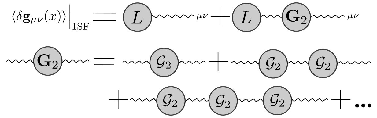
Figure 1: The 1SF metric diagrammatic expansion.

​​​​​ which is represented diagrammatically in Fig. 1. Note that here we use retarded boundary conditions for the propagators and the effective vertices, consistently with the fact that we are solving a classical equation in terms of initial boundary conditions. Moreover, given that $\delta\bm{g}_{\alpha\beta}$ is a perturbation on the background spacetime, it satisfies

$$\left(\delta^{\alpha}_{\mu}\bar{g}^{\beta\gamma}-\frac{1}{2}\bar{g}^{\alpha\beta}\delta^{\gamma}_{\mu}\right)\overline{\nabla}_{\gamma}\langle\delta\bm{g}_{\alpha\beta}(x)\rangle=0\,,$$ (84)

which is a non-trivial constraint on the final result. At leading order in the PM expansion, we can use the free light-body trajectory (53) to compute

$$\hskip-6.0pt\langle\delta\bm{g}_{\mu\nu}(x)\rangle\Big{|}_{\mathrm{1SF},\mathcal{O}(G_{\mathrm{N}})}\!\!\!\!=-16\pi G_{\mathrm{N}}\int\mathrm{\hat{d}}^{d}k\,e^{ik\cdot x}\,G^{(0)\mathrm{ret}}_{\mu\nu\alpha\beta}(k)\tilde{T}^{\alpha\beta}_{\mathrm{L}}(k^{\sigma})$$

$$\qquad=16\pi G_{\mathrm{N}}m_{\mathrm{L}}\left(v_{\mathrm{L}\mu}v_{\mathrm{L}\nu}+\frac{\eta_{\mu\nu}}{d-2}\right)\int\mathrm{\hat{d}}^{d-1}\vec{k}\,\frac{e^{-i\vec{k}\cdot\vec{r}_{\mathrm{L}}}}{|\vec{k}|^{2}}$$

$$\qquad\stackrel{{\scriptstyle d\to 4}}{{=}}\frac{2G_{\mathrm{N}}m_{\mathrm{L}}}{|\vec{r}_{\mathrm{L}}|}\left(2v_{\mathrm{L}\mu}v_{\mathrm{L}\nu}+\eta_{\mu\nu}\right)\,,$$ (85)

which is the linearized Schwarzschild metric generated by the light particle source with $r_{\mathrm{L}}^{\mu}=x^{\mu}-(x\cdot v_{\mathrm{L}})v_{\mathrm{L}}^{\mu}$.

While (83) provides an off-shell recursion for the metric, we can also consider the on-shell waveform. Performing the LSZ reduction in curved spacetime is subtle, as when considering the external wavefunctions of the asymptotic graviton state we can either take the plane-wave solution $\sim\bm{\varepsilon}_{\mu\nu}(k)\exp(ik\cdot x)$ [88] or the one that satisfies the linearized equations of motion [109, 110, 111]. Here we consider the first approach, constructing a convenient Newman-Penrose tetrad basis $(n^{\mu},\bar{n}^{\mu},\bm{\varepsilon}^{\mu},\bm{\bar{\varepsilon}}^{\mu})$ at null infinity where we project our asymptotic states.

Considering a detector with velocity $t^{\mu}$ placed at a spatial distance $r$ from the scattering event in the angular direction determined by $\hat{n}^{\mu}$ (with $\hat{n}\cdot\hat{n}=0$ and $\hat{n}\cdot t=-1$), we define $x^{\mu}=ut^{\mu}+r\hat{n}^{\nu}$ and take the limit $r\to+\infty$ for fixed $(u,\hat{n})$, obtaining the waveform recursion relation

$$\hskip-13.0pt\langle\delta\bm{g}^{1/|\vec{x}|}_{\mu\nu}(u,\hat{n})\rangle\Big{|}_{\mathrm{1SF}} \!\!\!\!\!\sim\frac{1}{4\pi|\vec{x}|}\int\!\mathrm{\hat{d}}\omega\,e^{-i\omega u}\,\mathcal{P}_{\mu\nu\alpha\beta}^{(d)}\tilde{T}^{\alpha\beta}(\omega\hat{n})\,,$$ (86)

in terms of the pseudo stress tensor [112, 113, 114]

$$\tilde{T}^{\alpha\beta}(\omega\hat{n}) =\mathcal{V}_{\mathrm{L}}^{\alpha\beta}(\omega\hat{n})$$ (87)

$$\hskip-20.0pt+\int\mathrm{\hat{d}}^{d}k_{1}\,\,\mathcal{G}_{2,\mathrm{ret}}^{\alpha\beta\lambda\rho}(\omega\hat{n},k_{1})\,G^{(0)\mathrm{ret}}_{\lambda\rho\xi\zeta}(k_{1})\mathcal{V}^{\xi\zeta}_{\mathrm{L}}(k_{1})+\dots\,,$$

At leading order in $G_{\mathrm{N}}$ we obtain

$$\hskip-10.0pt\langle\bm{\bar{\varepsilon}}^{\mu}\bm{\bar{\varepsilon}}^{\nu}\delta\bm{g}^{1/|\vec{x}|}_{\mu\nu}(u,\hat{n})\rangle\Big{|}_{\mathrm{1SF},\mathcal{O}(G_{\mathrm{N}})}=\frac{4G_{\mathrm{N}}}{|\vec{x}|}\frac{m_{\mathrm{L}}\left(\bm{\bar{\varepsilon}}\cdot v_{\mathrm{L}}\right)^{2}}{(\hat{n}\cdot v_{\mathrm{L}})}\,,$$ (88)

which is the linear memory contribution due to the light particle. At 1SF order, given that our perturbation is on the background spacetime, the BMS frame – which we refer to as the “intrinsic self-force BMS frame” – is adapted to the background metric. Technically speaking, by including the background metric after the shift (III), at this order the BMS frame corresponds to the usual amplitude or MPM intrinsic frame [115, 113, 116, 117, 118, 114, 119, 120, 121, 122, 123, 124, 125]. However, in general it might be different beyond 1SF order [126].

At order $G_{\mathrm{N}}^{2}$ and beyond, the 1SF metric (83) becomes sensitive to the graviton 2-point (time-ordered) correlator

$$\hskip-10.0pt\langle\mathcal{T}\delta\bm{g}_{\mu\nu}(x)\delta\bm{g}_{\alpha\beta}(y)\rangle\Big{|}_{\mathrm{1SF}}\!\!\!\!\!=\!\frac{1}{(-\bar{g})}\frac{\delta^{2}\mathbf{W}^{\mathrm{1SF}}[J]}{i^{2}\delta\mathbf{J}^{\mu\nu}(x)\delta\mathbf{J}^{\alpha\beta}(y)}\Big{|}_{\mathbf{J}=0}\!\!\,,$$ (89)

which generalizes the usual definition of the graviton propagator on the background spacetime by including the recoil contributions of the heavy source. Note that this correlator obeys the gauge condition (84) on either coordinate $(x,y)$ and its associated index group.

An important amount of work has been done in relating the result of BH perturbation theory in vacuum with the PM expansion at 1SF order using both the MST formalism and the Nekrasov-Shatashvili partition function [127, 128, 129, 130, 59, 63, 69, 131, 132, 133, 134, 135, 14, 136]. The advantage of sticking with the 1SF waveform – neglecting therefore 2SF contributions and beyond – is that its analytic structure is expected to be simpler [130, 133, 120, 135, 125, 136], as it obeys a single differential equation (60). However, there are still three outstanding puzzles. The first is how the boundary conditions for the wave scattering problem for BH vacuum solutions – involving the horizon – are related to the ones for particle-generated backgrounds with the recoil contribution. The second is how to perform the matching with a point-particle description beyond 1SF order, which is needed already for the one-loop Compton in Kerr. The final puzzle is how to better connect the analytic resummation of the Post-Minkowskian series with strong-field effects both for the 1-point and 2-point function, exploiting the simplicity of the 1SF theory. As an effort in these directions, we will now study the analytic properties of the Compton amplitude at loop level.

V Kerr Compton amplitude: Post-Minkowskian vs self-force

In this section, we study the 1SF Compton amplitude appearing in the waveform recursion relation (86) and compare it with the one-loop Compton amplitude for Kerr at quadratic order in spin. Physically, for the waveform only the wave regime of the Compton is relevant, which we will explore in detail emphasizing the analytic structure and the relation between the PM and GSF expansion. Finally, to understand the role of the resummation in the recursion relation, we will also consider the geometric optics regime of the 1SF Compton at all loop orders, uncovering the relation between the radius of convergence of the PM expansion and the critical angular momentum corresponding to the photon ring radius.

The wave regime: 1SF Compton recursion relation

Let us now compute the 1SF Compton $\mathcal{M}_{1\to 1}$ defined from $\langle\mathcal{T}\delta\bm{g}_{\mu\nu}(x)\delta\bm{g}_{\alpha\beta}(y)\rangle$ in (89), discussing its relation to the flat space classical Compton amplitude $\mathcal{A}_{2\to 2}$ derived from the LSZ reduction of $\langle\mathcal{T}h_{\mu\nu}(x)h_{\alpha\beta}(y)\rangle$. The 1SF Compton (resp. flat space Compton) at $\mathcal{O}(G_{\mathrm{N}}^{n+1})$ is denoted by $\mathcal{M}^{(n)}_{1\to 1}$ (resp. $\mathcal{A}^{(n)}_{2\to 2}$) and we strip off the delta function $\hat{\delta}(v_{\mathrm{H}}\cdot k_{1}+v_{\mathrm{H}}\cdot k_{2})$ (resp. $\hat{\delta}^{4}(k_{1}+k_{2}+p_{\mathrm{H}}+p^{\prime}_{\mathrm{H}})$).

As explained in section III, the corresponding 1-point functions are related by

$$\langle\kappa h_{\mu\nu}\rangle=\bar{H}_{\mu\nu}+\langle\lambda\delta\bm{g}_{\mu\nu}\rangle\,,$$ (90)

where $\bar{H}_{\mu\nu}$ is the background field. Crucially, this shift has direct implications also for the 2-point function, introducing a non-trivial relation between the 1SF Compton and the flat space Compton beyond tree-level.

Now we turn our attention to the 1SF Compton amplitude $\mathcal{M}_{1\to 1}(k_{1},k_{2})$. We start by focusing on the so-called wave or Born regime, which corresponds to the kinematic region $|\vec{q}|,\omega\ll m_{\mathrm{H}}$ where

$$|\vec{q}|=|\vec{k}_{1}+\vec{k}_{2}|=\sqrt{-q^{2}}\,,\quad\omega=v_{\mathrm{H}}\cdot k_{1}=-v_{\mathrm{H}}\cdot k_{2}\;,$$ (91)

denotes the exchanged momentum and frequency of external graviton momenta, respectively. At tree-level, we can directly combine the single insertion of the background and the recoil vertex to obtain

$$\hskip-7.11317pti\mathcal{M}^{(0)}_{1\to 1}(k_{1},k_{2}) =\bm{\varepsilon}_{\mu\nu}(k_{1})\mathcal{G}_{2}^{\mu\nu\alpha\beta}(k_{1},k_{2})\bm{\varepsilon}_{\alpha\beta}(k_{2})$$ (92)

$$\hskip-5.0pt\stackrel{{\scriptstyle\mathcal{O}(G_{\mathrm{N}})}}{{=}}\frac{4\pi iG_{\mathrm{N}}m_{\mathrm{H}}\mathcal{J}_{0}^{2}}{|\vec{q}|^{2}\left(k_{1}\cdot v_{\mathrm{H}}\right)^{2}}\sum_{n=0}^{2}\frac{1}{n!}\left(\frac{\mathcal{J}_{1}}{\mathcal{J}_{0}}\right)^{n}\,,$$

where the spin multipoles are defined as

$$\mathcal{J}_{0}=-2v_{\mathrm{H}}\cdot F_{1}\cdot F_{2}\cdot v_{\mathrm{H}}\,,$$ (93)

$$2i\mathcal{J}_{1}=2m_{\mathrm{H}}(k_{1}\cdot F_{2}\cdot v_{\mathrm{H}})(\bar{S}_{\mathrm{H}}\cdot F_{1})$$ (94)

$$\qquad-m_{\mathrm{H}}(\left(k_{1}-k_{2}\right)\cdot v_{\mathrm{H}})(\bar{S}_{\mathrm{H}}\cdot F_{1}\cdot F_{2})+(1\leftrightarrow 2)\,,$$

in terms of the field strength $F^{\mu\nu}_{i}(k_{i})=2k^{[\mu}_{i}\bm{\varepsilon}^{\nu]}_{i}(k_{i})$. Therefore, we obtain a correspondence with the usual spinning flat space Compton at tree-level order [138, 59]

$$\frac{1}{2m_{\mathrm{H}}}\mathcal{A}^{(0)}_{2\to 2}(k_{1},k_{2}) \mathrel{\stackunder[2pt]{\stackon[4pt]{=}{$\scriptscriptstyle\hbar\to 0$}}{$\scriptscriptstyle\varepsilon_{\mu\nu}\to\bm{\varepsilon}_{\mu\nu}$}}\mathcal{M}^{(0)}_{1\to 1}(k_{1},k_{2})\,,$$ (95)

where the heavy particle momentum is parametrized as

$$p^{\mu}_{\mathrm{H}}=m_{\mathrm{H}}v^{\mu}_{\mathrm{H}}-\frac{q^{\mu}}{2}\,,\qquad(p^{\prime})^{\mu}_{\mathrm{H}}=-m_{\mathrm{H}}v^{\mu}_{\mathrm{H}}-\frac{q^{\mu}}{2}\,.$$ (96)

Diagrammatically, the recoil contribution can be identified with the effective contact vertex coming from the heavy mass expansion of the following flat space diagrams

$$\leavevmode\hbox to0pt{\vbox to0pt{\text{[drawing]}}}\Bigg{|}_{\mathcal{O}(G_{\mathrm{N}})} H$$ (97)

$$\hskip-8.0pt\sim\Bigg{[}\leavevmode\hbox to0pt{\vbox to0pt{\text{[drawing]}}}\!\!+\!\!\leavevmode\hbox to0pt{\vbox to0pt{\text{[drawing]}}}\!\!+\!\!\leavevmode\hbox to0pt{\vbox to0pt{\text{[drawing]}}}\Bigg{]}\Bigg{|}_{\mathcal{O}(m_{\mathrm{H}}^{2})},$$

with the equality holding on-shell. The background insertion, on the other hand, contains an explicit propagator and is given on-shell by the usual t-channel contribution

$$\hskip-7.0pt\leavevmode\hbox to0pt{\vbox to0pt{\text{[drawing]}}}\Bigg{|}_{\mathcal{O}(G_{\mathrm{N}})}\!\!\!\sim\!\!\!\leavevmode\hbox to0pt{\vbox to0pt{\text{[drawing]}}}\Bigg{|}_{\mathcal{O}(m_{\mathrm{H}}^{2})}. G$$ (98)

The next object to study is the 1SF Compton amplitude at one-loop, which is given by the combination of the single background vertex at $\mathcal{O}(G_{\mathrm{N}}^{2})$ and the iteration of the combined background and recoil insertion at $\mathcal{O}(G_{\mathrm{N}})$

$$i\mathcal{M}^{(1)}_{1\to 1}(k_{1},k_{2})=\bm{\varepsilon}_{\mu\nu}(k_{1})\mathcal{G}_{2}^{\mu\nu\alpha\beta}(k_{1},k_{2})\bm{\varepsilon}_{\alpha\beta}(k_{2})+I^{\mathrm{s-iter}}_{1\to 1}$$

$$I^{\mathrm{s-iter}}_{1\to 1}=\int\hat{\mathrm{d}}^{d}\ell_{1}\,\bm{\varepsilon}_{\mu\nu}(k_{1})\mathcal{G}_{2}^{\mu\nu\rho\lambda}(k_{1},\ell_{1})$$

$$\qquad\qquad\qquad\qquad\times\frac{i\mathcal{P}^{(d)}_{\rho\lambda\xi\zeta}}{\ell_{1}^{2}+i\epsilon}\mathcal{G}_{2}^{\xi\zeta\alpha\beta}(\ell_{1},k_{2})\bm{\varepsilon}_{\alpha\beta}(k_{2})\,,$$ (99)

where we parametrize the external graviton legs as

$$k_{1}^{\mu}=k^{\mu}+\frac{q^{\mu}}{2}\,,\quad k_{2}^{\mu}=-k^{\mu}+\frac{q^{\mu}}{2}\,,\quad v_{\mathrm{H}}\cdot q=0\,.$$ (100)

together with the gauge choice $v_{\mathrm{H}}\cdot\bm{\varepsilon}_{i}=0$.

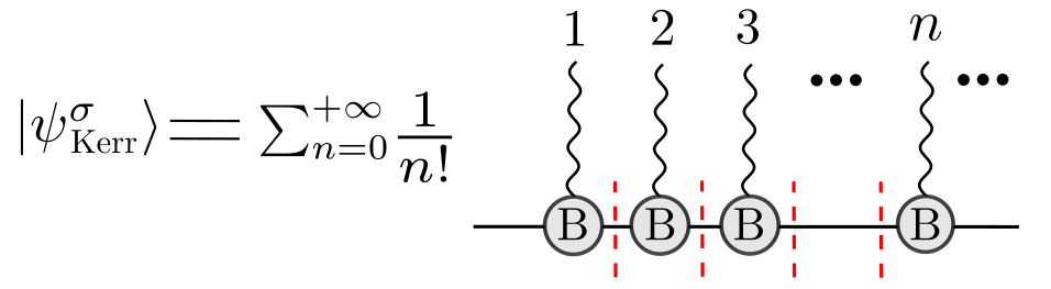
Figure 2: The Kerr background $\left|\psi_{\mathrm{Kerr}}^{\sigma}\right\rangle$ is described by an off-shell coherent state of virtual gravitons.

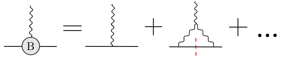
Figure 3: The stress tensor for Kerr spacetime is given by a sum of perturbative diagrams.

The 1SF Compton at one-loop is of the form

$$\hskip-6.0pti\mathcal{M}^{(1)}_{1\to 1}(k_{1},k_{2})\!=\!\frac{1}{2m_{\mathrm{H}}}\!\Big{[}\bm{c}_{\scriptscriptstyle\Box}(k,q,\bar{S}_{\mathrm{H}})(\mathcal{I}_{\scriptscriptstyle\Box}(\omega,q)+\mathcal{I}_{\scriptscriptstyle\boxtimes}(\omega,q))$$

$$\qquad\qquad\qquad\qquad\quad+\bm{c}_{\scriptscriptstyle\bigtriangleup}(k,q,\bar{S}_{\mathrm{H}})\,\mathcal{I}_{\scriptscriptstyle\bigtriangleup}(q)$$

$$\qquad\qquad\qquad\qquad\quad+\bm{c}_{\scriptscriptstyle\rotatebox[origin={c}]{-90.0}{$\between$}}(k,q,\bar{S}_{\mathrm{H}})\,\mathcal{I}_{\scriptscriptstyle\rotatebox[origin={c}]{-90.0}{$\between$}}(\omega)\Big{]}\,,$$ (101)

where we separate the analytic dependence on $q^{2}$ in the coefficients from the master integrals $(\mathcal{I}_{\scriptscriptstyle\Box},\mathcal{I}_{\scriptscriptstyle\boxtimes},\mathcal{I}_{\scriptscriptstyle\bigtriangleup},\mathcal{I}_{\scriptscriptstyle\rotatebox[origin={c}]{-90.0}{$\between$}})$, which are readily evaluated around $d=4-2\epsilon$

$$\hskip-4.26773pt\mathcal{I}_{\scriptscriptstyle\Box}(q,\omega)+\mathcal{I}_{\scriptscriptstyle\boxtimes}(q,\omega)\simeq\frac{i}{2\pi m_{\mathrm{H}}}\int\frac{\hat{\mathrm{d}}^{d-1}\vec{\ell}}{|\vec{k}_{1}-\vec{\ell}|^{2}|\vec{k}_{2}+\vec{\ell}|^{2}(\omega^{2}-|\vec{\ell}|^{2})}$$

$$\qquad\qquad\qquad\quad\!\stackrel{{\scriptstyle d=4-2\epsilon}}{{\simeq}}-\frac{i}{16\pi^{2}m_{\mathrm{H}}\omega|\vec{q}|^{2}}\Big{[}\frac{1}{\epsilon}-\operatorname{log}(|\vec{q}|^{2})\Big{]}\,,$$

$$\mathcal{I}_{\scriptscriptstyle\bigtriangleup}(q)\!=\!\frac{1}{m_{\mathrm{H}}}\int\hat{\mathrm{d}}^{d}\ell\,\frac{\delta(v_{H}\cdot\ell)}{\ell^{2}(\ell-q)^{2}}\stackrel{{\scriptstyle d=4-2\epsilon}}{{\simeq}}\frac{1}{16\pi m_{\mathrm{H}}|\vec{q}|}\,,$$ (102)

$$\mathcal{I}_{\scriptscriptstyle\rotatebox[origin={c}]{-90.0}{$\between$}}(\omega)\!=\!\frac{i}{m_{\mathrm{H}}}\int\hat{\mathrm{d}}^{d}\ell\,\,\frac{\delta\left(v_{\mathrm{H}}\cdot\left(\ell-k\right)\right)}{\ell^{2}}\!\!\stackrel{{\scriptstyle d=4-2\epsilon}}{{\simeq}}\!\!-\frac{\pi\omega}{m_{\mathrm{H}}}\,.$$

The value of these coefficients in the wave regime – except for the s-channel bubble term $\bm{c}_{\scriptscriptstyle\rotatebox[origin={c}]{-90.0}{$\between$}}$ – can be found in appendix D, and are determined by the background insertion and its iteration. We leave the detailed evaluation of the iteration of the recoil contribution for the future, exploring here only its general structure and the relation between the flat and curved space Compton amplitudes.

We now discuss the interpretation of (101). The background contribution arises entirely from the quadratic graviton action (IV), and it has the interpretation of a graviton scattering off a fixed Kerr background. This is manifest from the equations of motion (64) in the absence of the recoil and the source term, and it can also be verified by constructing the off-shell coherent state describing the Kerr black hole up to quadratic order in spin. Following Refs. [139, 140], we define (see Fig. 3)

$$\hskip-8.0pt\left|\psi_{\mathrm{Kerr}}^{\sigma}\right\rangle\sim\exp\Big{[}\int\frac{\hat{\mathrm{d}}^{d}\ell_{1}}{\ell_{1}^{2}+i\epsilon}\hat{\delta}\left(2p_{H}\cdot\ell_{1}\right)$$

$$\qquad\qquad\quad\times i\varepsilon^{\sigma}_{\mu\nu}(\ell_{1})\tilde{T}_{\mathrm{H},\mathrm{spin}}^{\mu\nu}(\ell_{1})A_{\sigma}^{\dagger}(\ell_{1})\Big{]}|p_{H}\rangle\,,$$ (103)

where $A_{\sigma}^{\dagger}(\ell_{1})$ is a placeholder for the operator creating a virtual graviton and $\tilde{T}_{\mathrm{H},\mathrm{spin}}^{\mu\nu}(\ell_{1})$ is the momentum space effective stress tensor for a massive spinning particle. While the linearized term has been discussed earlier (45), building on Refs. [23, 24, 25] we can identify higher-loop contributions to the effective stress tensor with the diagrams in Fig. 3 where an off-shell graviton is emitted from the massive spinning particle. Using this intuition, we can verify that the tree-level background contribution arise from gluing a single insertion of the coherent state vertex at $G_{\mathrm{N}}$ with the wiggly line representing the graviton; see (98). At order $G_{\mathrm{N}}^{2}$, we need to combine both the single background insertion and its iteration to get a correspondence with flat space diagrams

$$\leavevmode\hbox to0pt{\vbox to0pt{\text{[drawing]}}}+\leavevmode\hbox to0pt{\vbox to0pt{\text{[drawing]}}} G G G$$ (104)

$$\stackrel{{\scriptstyle\mathcal{O}(G_{\mathrm{N}}^{2})}}{{\sim}}\leavevmode\hbox to0pt{\vbox to0pt{\text{[drawing]}}}+\leavevmode\hbox to0.4pt{\vbox to0.4pt{\text{[drawing]}}}\,, \mathcal{\tilde{A}}^{\scalebox{0.6}{(0)}}_{3} \mathrm{B} \mathrm{B} \mathrm{B} \mathcal{\tilde{A}}^{\scalebox{0.6}{(0)}}_{4}$$

where we introduced the 3-point $\mathcal{\tilde{A}}^{(0)}_{3}$ and 4-point $\mathcal{\tilde{A}}^{(0)}_{4}$ graviton tree-level amplitudes (see e.g. Ref. [141]).

The iteration term of the 1SF Compton (V), including both the background and the recoil, then corresponds to the s-channel iteration of some classical piece of the tree-level flat space Compton amplitude $\mathcal{A}^{(0)}_{2\to 2}$

$$I^{\mathrm{s-iter}}_{1\to 1}=\leavevmode\hbox to0pt{\vbox to0pt{\text{[drawing]}}}\Bigg{|}_{\mathcal{O}(G_{\mathrm{N}}^{2})} \mathcal{G}_{2} \mathcal{G}_{2} k_{1} \ell_{1} k_{2}$$ (105)

$$\subseteq I^{\mathrm{s-iter}}_{2\to 2}=\leavevmode\hbox to0pt{\vbox to0pt{\text{[drawing]}}}\Bigg{|}_{\mathcal{O}(m_{\mathrm{H}}^{3})}\,, \mathcal{A}^{\scalebox{0.6}{(0)}}_{4} \mathcal{A}^{\scalebox{0.6}{(0)}}_{4} k_{1} k_{2} p_{\mathrm{H}}+k_{1}-\ell_{1} \ell_{1}$$

in line with the expectations from (97) and (98). However, we find that the iteration $I^{\mathrm{s-iter}}_{1\to 1}$ differs from the flat space s-channel iteration $I^{\mathrm{s-iter}}_{2\to 2}$

$$\hskip-3.0ptI^{\mathrm{s-iter}}_{1\to 1}-\frac{I^{\mathrm{s-iter}}_{2\to 2}}{2m_{\mathrm{H}}}\!\stackrel{{\scriptstyle\mathcal{O}(m_{\mathrm{H}}^{2})}}{{\sim}}\!\frac{1}{2m_{\mathrm{H}}}(\bm{c}_{\scriptscriptstyle\rotatebox[origin={c}]{-90.0}{$\between$}}-c^{s\text{-cut}}_{\scriptscriptstyle\rotatebox[origin={c}]{-90.0}{$\between$}})\mathcal{I}_{\scriptscriptstyle\rotatebox[origin={c}]{-90.0}{$\between$}}\,,$$ (106)

by contact terms, encoded in the s-channel curved $\bm{c}_{\scriptscriptstyle\rotatebox[origin={c}]{-90.0}{$\between$}}$ and flat $c^{s\text{-cut}}_{\scriptscriptstyle\rotatebox[origin={c}]{-90.0}{$\between$}}$ bubble coefficients. We have also demonstrated this with a detailed one-loop calculation in electrodynamics, in the absence of spin.

The one-loop mismatch (106) is not surprising, because the 1SF recoil term includes only some of the heavy-mass expanded pieces of the s-channel and u-channel diagram contributing to the tree-level Compton; see (97). Moreover, it is worth stressing that the curved space gauge condition (84) is mixing – because of the covariant derivative – both the tree (92) and one-loop (V) 1SF Compton, and therefore it is expected that the curved and flat space Compton amplitudes do not agree with each other when expressed in terms of flat space kinematics. We will come back to this point at the end of the next section, showing how to reconcile the difference between these amplitudes.

Figure 4: The generic cut configurations contributing to the classical one-loop flat space Compton.

1SF Compton vs flat space Compton at one-loop

The classical one-loop Compton amplitude in flat space receives contribution both from the t-channel and s-channel cut configurations, as shown in Fig. 4. We will study the analytic structure of the amplitude in the wave regime, evaluating the box, crossed box and triangle coefficients with generalized unitarity [143, 144, 145, 146]. In this discussion, we do not consider the contact terms arising from the s-channel bubble coefficients, as it would require the 4-point quantum spinning Compton amplitude. A detailed analysis of these contributions is left to future work. Here, we focus instead on comparing the curved and flat space Compton amplitude at one-loop order.

The classical one-loop Compton amplitude can be written in the form

$$i\mathcal{A}^{(1)}_{2\to 2}=c_{\scriptscriptstyle\Box}\mathcal{I}_{\scriptscriptstyle\Box}+c_{\scriptscriptstyle\boxtimes}\mathcal{I}_{\scriptscriptstyle\boxtimes}+c_{\scriptscriptstyle\bigtriangleup}\mathcal{I}_{\scriptscriptstyle\bigtriangleup}+c^{s\text{-cut}}_{\scriptscriptstyle\rotatebox[origin={c}]{-90.0}{$\between$}}\mathcal{I}_{\scriptscriptstyle\rotatebox[origin={c}]{-90.0}{$\between$}}+\mathcal{O}(m^{4}_{\mathrm{H}})\,,$$

$$\qquad\qquad\qquad c_{\scriptscriptstyle\bigtriangleup}=c_{\scriptscriptstyle\bigtriangleup}^{{\scriptscriptstyle\Box}\text{-cut}}+c_{\scriptscriptstyle\bigtriangleup}^{{\scriptscriptstyle\boxtimes}\text{-cut}}+c_{\scriptscriptstyle\bigtriangleup}^{{\scriptscriptstyle\bigtriangleup}\text{-cut}}\;,$$ (107)

where we have distinguished the contributions coming from different cut configurations. The related coefficients of the master integrals $(c_{\scriptscriptstyle\Box},c_{\scriptscriptstyle\boxtimes},c_{\scriptscriptstyle\bigtriangleup})$ in the wave regime can be found in appendix D, while the master integrals have been evaluated earlier in (102).

We start by considering the following cuts

$$\leavevmode\hbox to0.4pt{\vbox to0.4pt{\text{[drawing]}}},\leavevmode\hbox to0.4pt{\vbox to0.4pt{\text{[drawing]}}} \mathcal{\tilde{A}}^{\scalebox{0.6}{(0)}}_{3} \mathcal{\tilde{A}}^{\scalebox{0.6}{(0)}}_{3} \mathcal{A}^{\scalebox{0.6}{(0)}}_{3} \mathcal{A}^{\scalebox{0.6}{(0)}}_{3} k_{1} k_{2} \ell_{1} \ell_{2} \mathcal{A}^{\scalebox{0.6}{(0)}}_{3} \mathcal{A}^{\scalebox{0.6}{(0)}}_{3} \mathcal{\tilde{A}}^{\scalebox{0.6}{(0)}}_{4} k_{1} k_{2} \ell_{1} \ell_{2}$$

which require the 3-point $\mathcal{\tilde{A}}^{(0)}_{3}$ and 4-point $\mathcal{\tilde{A}}^{(0)}_{4}$ graviton tree-level amplitudes [141] as well as the 3-point amplitude for two massive spinning particles expanded to quadratic order in spin [35, 64, 56]

$$\begin{split}&\quad\qquad\mathcal{A}_{3}^{(0)}(k)=-i\kappa m_{\mathrm{H}}^{2}(v_{\mathrm{H}}\cdot\varepsilon)(\text{w}\cdot\varepsilon)\,,\\ &\hskip 8.5359pt\text{w}^{\mu}=v_{\mathrm{H}}^{\mu}+i\epsilon^{\mu\nu\rho\sigma}k_{\nu}v_{\mathrm{H}\rho}a_{\mathrm{H}\sigma}+\frac{1}{2}(k\cdot a_{\mathrm{H}})^{2}v_{\mathrm{H}}^{\mu}\;,\end{split}$$ (108)

where $k^{\mu}$ is the momentum of the incoming graviton leg and $a^{\mu}_{\mathrm{H}}$ is the normalized spin vector associated to the massive spinning legs. The result is then projected into a suitable basis with the FIRE6 [149] program, distinguishing between triangle topologies coming from each numerator after IBP. Importantly, here we have discarded t-channel bubbles, which are mass suppressed as compared to the other topologies in (V). Moreover, we notice that the t-channel bubbles appearing from the IBP reduction of the box, crossed box and triangle numerators cancel through quadratic order in spin.

To make a connection with the earlier analysis of the 1SF amplitude, we note that both the triangle coefficient, i.e. $c_{\scriptscriptstyle\bigtriangleup}$, and the box and crossed box coefficients $c_{\scriptscriptstyle\Box}=c_{\scriptscriptstyle\boxtimes}$ are in agreement with the single insertion of the background vertex and its iteration by formally replacing $\varepsilon_{\mu\nu}\to\bm{\varepsilon}_{\mu\nu}$ in such coefficients. Physically, this means that the one-loop flat and curved space Compton have the same high-energy behavior $|\vec{q}|\ll\omega$.

Finally, the s-channel bubble coefficient $c^{s\text{-cut}}_{\scriptscriptstyle\rotatebox[origin={c}]{-90.0}{$\between$}}$ – which encodes the soft behavior as $\omega\ll|\vec{q}|$ – is only partially reproduced (106) by the corresponding piece from the iteration of the background and recoil insertion $\bm{c}_{\scriptscriptstyle\rotatebox[origin={c}]{-90.0}{$\between$}}$, consistently with the expectations and our previous comparison with the one-loop Compton in electrodynamics [142]. Indeed, already at tree-level order the 1SF recoil insertion – which gives a contact term analogous to the bubble coefficient – was required to recover the full Compton, and here 2SF recoil contributions are needed at one-loop.

The question then becomes: how can we provide a precise connection between the curved space and flat space Compton at one-loop and beyond? Considering the action in (58) and setting $m_{\mathrm{L}}=0$ (focusing only on the Compton for the heavy source here) yields

$$\mathcal{S}^{\mathrm{spin}}_{\mathrm{eff}}[\delta\bm{g};\{\bar{H}^{k}\}]\Big{|}_{m_{\mathrm{L}}=0}\hskip-5.0pt=\lambda^{2}\mathbf{S}^{\mathrm{spin},\mathrm{1SF}}_{\mathrm{GR}+\mathrm{recoil}}[(\delta\bm{g})^{2};\{\bar{H}^{k}\}]$$ (109)

$$\qquad\quad+\lambda^{3}\mathbf{S}^{\mathrm{spin},\mathrm{2SF}}_{\mathrm{GR}+\mathrm{recoil}}[(\delta\bm{g})^{3};\{\bar{H}^{k}\}]$$

$$\qquad\quad+\dots+\lambda^{n+1}\mathbf{S}^{\mathrm{spin},\mathrm{nSF}}_{\mathrm{GR}+\mathrm{recoil}}[(\delta\bm{g})^{n+1};\{\bar{H}^{k}\}]+\dots\,.$$

We now see that the 1SF Compton is uniquely identified by the 1SF graviton and recoil action, but when computing the flat space Compton the shift (90) introduces a new 1-point function source which will couple to higher SF contributions. Note that this is not a field redefinition – under which the S-matrix would be invariant – because it introduces additional contributions from the background field in the path integral. Focusing our attention to the 1SF and 2SF action in (109), we obtain

$$\mathcal{S}^{\mathrm{spin}}_{\mathrm{eff}}[h;\{\bar{H}^{k}\}]\Big{|}_{m_{\mathrm{L}}=0}\sim\mathcal{S}^{\mathrm{spin},\mathrm{1SF}}_{\mathrm{GR}+\mathrm{recoil}}[h;\{\bar{H}^{k}\}]$$ (110)

$$\quad+\mathcal{S}^{\mathrm{spin},\mathrm{1SF}}_{\mathrm{GR}+\mathrm{recoil}}[h^{2};\{\bar{H}^{k}\}]+\mathcal{S}^{\mathrm{spin},\mathrm{2SF}}_{\mathrm{GR}+\mathrm{recoil}}[h;\{\bar{H}^{k}\}]$$

$$\quad+\mathcal{S}^{\mathrm{spin},\mathrm{2SF}}_{\mathrm{GR}+\mathrm{recoil}}[h^{2};\{\bar{H}^{k}\}]+\mathcal{S}^{\mathrm{spin},\mathrm{2SF}}_{\mathrm{GR}+\mathrm{recoil}}[h^{3};\{\bar{H}^{k}\}]+\dots\,,$$

giving new one-loop diagrams that directly mix the 1SF and 2SF contributions. Computing these diagrams explicitly would not only confirm our expectations, but also offer an alternative route to construct the full classical one-loop spinning Compton amplitude in flat space.

Given the simplicity of the background insertion and its dominance in the eikonal regime, we now study the behavior of the 1SF loop-level Compton by expanding the wave regime result in powers of $|\vec{q}|\ll\omega$. At tree-level, we recover the $t$-channel exchange contribution in (98), since all the contact terms coming from the recoil operator are suppressed. At one-loop order, we find a compact expression for the master coefficients at leading order in the expansion $|\vec{q}|/\omega\ll 1$

$$c_{\scriptscriptstyle\Box}^{\text{eik}}=c_{\scriptscriptstyle\boxtimes}^{\text{eik}}=256\pi^{3}G_{\mathrm{N}}^{2}m_{\mathrm{H}}^{4}\omega^{2}(\bm{\varepsilon}_{1}\cdot\bm{\varepsilon}_{2})^{2}\Big{(}2\omega^{2}-2i\omega(l_{k}\cdot a_{\mathrm{H}})$$

$$\hskip 28.45274pt+\omega^{2}[(q\cdot a_{\mathrm{H}})^{2}-q^{2}a_{\mathrm{H}}^{2}]-q^{2}(k\cdot a_{\mathrm{H}})^{2}\Big{)}\,,$$ (111)

$$\hskip 7.11317ptc_{\scriptscriptstyle\bigtriangleup}^{\text{eik}}=-\pi^{3}G_{\mathrm{N}}^{2}m_{\mathrm{H}}^{4}(\bm{\varepsilon}_{1}\cdot\bm{\varepsilon}_{2})^{2}\Big{(}480\omega^{2}-640i\omega(l_{k}\cdot a_{\mathrm{H}})$$

$$\hskip 28.45274pt+380\omega^{2}[(q\cdot a_{\mathrm{H}})^{2}-q^{2}a_{\mathrm{H}}^{2}]-520q^{2}(k\cdot a_{\mathrm{H}})^{2}\Big{)}\,.$$

Unlike the wave regime, here only the triangles contribute to the classical dynamics, because the box and crossed box correspond to superclassical iterations of the tree-level eikonal phase. This is expected also from the optical theorem, as the imaginary part of the one-loop amplitude in the forward limit –which is divergent in this case– is related to the tree-level gravitational Compton cross section [55, 150, 151]. The first few subleading orders in the eikonal expansion have also been explored in Ref. [61] and can be interpreted as polarization-dependent corrections to the point particle dynamics, although the exponentiation breaks down in the full wave regime as discussed before. Exploiting the simplification of the geometric optics approximation is the goal of our next section.

The eikonal regime: an all order resummation

We now turn our attention to the 1SF Compton in the classical geometric optics regime $|\vec{q}|\ll\omega\ll m_{\mathrm{H}}$. We will show that this corresponds, as expected, to the null geodesic limit for the scattering of gravitons in Kerr. Following Ref. [152], we define the WKB approximation

$$\delta\bm{g}^{\mathrm{tr}}_{\alpha\beta}(x)=A_{\alpha\beta}(x,k(x),\hbar)e^{iI(x)/\hbar}\,,\quad k_{\mu}(x)=\overline{\nabla}_{\mu}I(x)\,,$$

$$A_{\alpha\beta}(x,k(x),\hbar)=A_{0\alpha\beta}(x,k(x))$$

$$\qquad\qquad\qquad\qquad+\hbar A_{1\alpha\beta}(x,k(x))+\mathcal{O}\left(\hbar^{2}\right)\,,$$ (112)

where $I$ is a real scalar function, $A_{\alpha\beta}$ is a complex amplitude and $\hbar$ is a small expansion parameter. Physically, taking $\hbar\to 0$ forces the saddle-point approximation and it is equivalent to having a large classical phase shift. Inserting (112) into the 1SF effective action (52), we obtain

$$\mathcal{S}^{\mathrm{spin},\mathrm{1SF}} \sim-\frac{1}{2\hbar^{2}}\int\mathrm{d}^{4}x\,\sqrt{-\bar{g}}\left[A^{\alpha\beta}\hat{\mathcal{D}}_{\alpha\beta}{}^{\gamma\delta}A_{\gamma\delta}+\mathcal{O}\left(\hbar\right)\right]\,,$$

$$\hat{\mathcal{D}}_{\alpha\beta}{}^{\gamma\delta} =\bar{g}^{\mu\nu}k_{\mu}(x)k_{\nu}(x)\left[\delta_{\alpha}^{\gamma}\delta_{\beta}^{\delta}-\frac{1}{2}\bar{g}_{\alpha\beta}\bar{g}^{\gamma\delta}\right]\,.$$ (113)

The effective action now depends on $I(x)$ (through $k(x)$) and $A_{\mu\nu}(x)$, and we have suppressed contributions which are subleading in the $\hbar\to 0$ limit. Considering the equations of motion for $A_{\mu\nu}$, we then obtain

$$\left(\bar{g}^{\mu\nu}k_{\mu}(x)k_{\nu}(x)\right)\left[A_{\alpha\beta}-\frac{1}{2}\bar{g}_{\alpha\beta}\bar{g}^{\gamma\delta}A_{\gamma\delta}\right]=0\,,$$ (114)

which, discarding the trivial solution $A_{\alpha\beta}=0$, implies

$$\bar{g}^{\mu\nu}(x)k_{\mu}(x)k_{\nu}(x)=0\,.$$ (115)

The latter is exactly the Hamilton-Jacobi equation for a point particle moving in the Kerr background $\bar{g}_{\mu\nu}$: indeed, defining the Hamiltonian

$$H(x,p)=\frac{1}{2}\bar{g}^{\mu\nu}(x)p_{\mu}p_{\nu}\,,$$ (116)

the condition (115) becomes equivalent to $H(x,\nabla I)=0$. This is a manifestation of the classical equivalence principle of GR, and it illustrates why the 1SF Compton amplitude in the geometric optics regime agrees with the probe amplitude for a massless scalar in the Kerr background generated by the heavy particle. Building on the amplitude-action relation [153, 154, 139, 155], we obtain

$$i\mathcal{M}^{\mathrm{eik}}_{1\to 1}(k_{1},k_{2})=2m_{\mathrm{H}}\omega^{2}$$

$$\quad\times\int\mathrm{d}^{2}b\,e^{-iq\cdot b}\left(e^{\frac{i}{\hbar}(I_{r}^{>}(\omega,b(J),a_{\mathrm{H}})+\pi J)}-1\right)\,,$$ (117)

where we find the resummed in $G_{\mathrm{N}}$ radial action

$$\hskip-7.0ptI_{r}^{>}(\omega,J,a_{\mathrm{H}})=\,-\pi J{}_{3}F_{2}\left(-\frac{1}{2},\frac{1}{6},\frac{5}{6};\frac{1}{2},1;\Lambda^{2}\right)$$ (118)

$$\quad\quad-\frac{3}{4}\sqrt{3}G_{\mathrm{N}}m_{\mathrm{H}}\omega\,G_{4,4}^{2,3}\left(\begin{array}[]{c}-\frac{1}{3},0,\frac{1}{3},1\\ 0,0,-\frac{1}{2},-\frac{1}{2}\\ \end{array}|-\Lambda^{2}\right)$$ (121)

$$\quad\quad-\frac{4a_{\mathrm{H}}\omega^{2}G_{\mathrm{N}}m_{\mathrm{H}}}{J}\,_{4}F_{3}\left(\frac{2}{3},1,1,\frac{4}{3};\frac{1}{2},\frac{3}{2},2;\Lambda^{2}\right)$$

$$\quad\quad-\frac{5\pi a_{\mathrm{H}}\omega^{3}G_{\mathrm{N}}^{2}m_{\mathrm{H}}^{2}}{J^{2}}\,_{3}F_{2}\left(\frac{7}{6},\frac{3}{2},\frac{11}{6};2,\frac{5}{2};\Lambda^{2}\right)\!+\!\mathcal{O}(a_{\mathrm{H}}^{2})\,,$$

written in terms of the variables

$$\Lambda=3\sqrt{3}\frac{G_{\mathrm{N}}m_{\mathrm{H}}\omega}{J}\,,\qquad J=b\omega\,.$$ (122)

This result generalizes eq. (3.8) of Ref. [156] to linear order in spin. As expected, the Fourier transform of the $n-$th loop contribution to $I_{r}^{>}$ is proportional to the 0SF master integral of the “fan” diagram [157, 147]

$$\hskip-12.0ptJ^{(L)}(q) =\int\left(\prod_{i=1}^{L}\frac{\mathrm{d}^{d}k_{i}}{\pi^{d/2}}\frac{\delta(k_{i}\cdot v_{\mathrm{H}})}{k_{i}^{2}}\right)\frac{(2\pi)^{L}}{[\sum_{j=1}^{L}k_{j}-q]^{2}}$$

$$\hskip-20.0pt\stackrel{{\scriptstyle d=4-2\epsilon}}{{\simeq}}(4\pi)^{L/2}\pi^{\frac{L+1}{2}}\frac{\Gamma\left(1-\frac{L}{2}+L\epsilon\right)}{\Gamma\left(\frac{L+1}{2}\right)}q^{L(1-2\epsilon)-2}\,.$$ (123)

The analytic expression (118) shows that there is a critical value of the angular momentum

$$J_{\mathrm{crit}}(\omega)=3\sqrt{3}G_{\mathrm{N}}m_{\mathrm{H}}\omega\,,$$ (124)

below which (i.e. for $\Lambda>1$) the radial action (118) develops an imaginary part, as explained also in Refs. [158, 156]. This is because a null geodesic falls into the black hole for $J<J_{\mathrm{crit}}(\omega)$, and therefore the initial wave is almost completely absorbed by the black hole in such a regime. The function $J_{\mathrm{crit}}(\omega)$ describes the separatrix between scattering and captured geodesics, which corresponds to the critical orbits which start at infinity and end with an infinite circular whirl at periastron distance (and their time-reversed counterpart) [10]. This can be considered a “smoking gun” signature of the strong-field nature of a black hole spacetime, and it is pleasing to see such a parameter arising from the perturbative series.

We now extend the consequences of the representation (118) at the level of observables. The scattering angle is

$$\chi(\omega,J,a_{\mathrm{H}})=-\frac{\partial I_{r}^{>}(\omega,J,a_{\mathrm{H}})}{\partial J}$$

$$\quad=\pi\,_{2}F_{1}\left(\frac{1}{6},\frac{5}{6};1;\Lambda^{2}\right)$$

$$\quad+\frac{4G_{\mathrm{N}}m_{\mathrm{H}}\omega}{J}\,_{3}F_{2}\left(\frac{2}{3},1,\frac{4}{3};\frac{3}{2},\frac{3}{2};\Lambda^{2}\right)$$

$$\quad-\frac{4a_{\mathrm{H}}\omega^{2}G_{\mathrm{N}}m_{\mathrm{H}}}{J^{2}}\,_{4}F_{3}\left(\frac{2}{3},1,1,\frac{4}{3};\frac{1}{2},\frac{1}{2},2;\Lambda^{2}\right)$$

$$\quad-\frac{10\pi a_{\mathrm{H}}\omega^{3}G_{\mathrm{N}}^{2}m_{\mathrm{H}}^{2}}{J^{3}}\,_{3}F_{2}\left(\frac{7}{6},\frac{3}{2},\frac{11}{6};1,\frac{5}{2};\Lambda^{2}\right)\,,$$ (125)

while the periastron advance reads, using the scattering-to-bound dictionary [159, 160, 161],

$$\Delta\Phi(\omega,J,a_{\mathrm{H}})=\chi(\omega,J,a_{\mathrm{H}})+\chi(\omega,-J,-a_{\mathrm{H}})$$

$$\quad=2\pi\,_{2}F_{1}\left(\frac{1}{6},\frac{5}{6};1;\Lambda^{2}\right)$$

$$\quad-\frac{20\pi a_{\mathrm{H}}\omega^{3}G_{\mathrm{N}}^{2}m_{\mathrm{H}}^{2}}{J^{3}}\,_{3}F_{2}\left(\frac{7}{6},\frac{3}{2},\frac{11}{6};1,\frac{5}{2};\Lambda^{2}\right)\,.$$ (126)

Interestingly, the separatrix $J_{\mathrm{crit}}(\omega)$ provides a critical curve in phase space $(\omega,J,a_{\mathrm{H}})$ which not only corresponds to the phase transition between scattering and captured geodesics, but it also provides crucial insights into the resummation through the singular behavior of observables [15]. Expanding around the separatrix

$$J=J_{\mathrm{crit}}(\omega)+\delta J\,,\quad$$ (127)

we find from (V) and (V)

$$\chi(\omega,J,a_{\mathrm{H}}) \stackrel{{\scriptstyle J\to J_{\mathrm{crit}}}}{{\sim}}-\log\left(\frac{\delta J}{J_{\mathrm{crit}}(\omega)}\right)-\frac{2a_{\mathrm{H}}\omega}{\delta J}\,,$$

$$\Delta\Phi(\omega,J,a_{\mathrm{H}}) \stackrel{{\scriptstyle J\to J_{\mathrm{crit}}}}{{\sim}}-\log\left(\frac{\delta J}{J_{\mathrm{crit}}(\omega)}\right)-\frac{2a_{\mathrm{H}}\omega}{\delta J}\,.$$ (128)

The same logarithmic divergence was identified for the scattering case in Refs. [9, 15]; here we find a similar structure for the bound case and we identify the related spin correction for Kerr black holes. It would be interesting to improve resummation methods for the PM expansion of spinning bound observables, perhaps building on what has been achieved for the scattering case [9, 15, 11].

VI Conclusions and future directions

The perturbative amplitude approach has successfully begun integrating into the gravitational wave program to enhance our understanding of compact binary systems. An important milestone in this direction is to explore the resummation of the Post-Minkowskian series, for example adapting tools from the gravitational self-force program. In this work, we have extended the spinless self-force approach in Refs. [16, 17, 18] to the case of Kerr black holes up to quadratic in spin order using the worldline formulation introduced in Ref. [76].

Our first step was to study the Myers–Perry metric and its relation with the amplitude approach for massive spinning particles, as well as the extension to $d$ dimensions of the linearized stress-energy tensor associated with the Kerr solution. This allows one to set up a dimensional regularization scheme for the spinning self-force EFT, whose action we have derived by expanding the trajectory and the Grassmann variables around their background value. Given that the spin tensor is proportional to the mass, we find that spin effects are suppressed (resp. enhanced) for the light-body (resp. heavy body).

At 0SF order, we recover the well-known fact that the self-force EFT describes only spinless geodesics in Kerr. At 1SF order, we find that only linear in spin corrections to the light-body degrees of freedom are relevant and – as in the spinless case – we can integrate out the heavy dynamics in terms of a non-local effective action (50), which includes novel spinning recoil contributions.

Remarkably, the 1SF action is only a function of the dynamical graviton field, which allows to study the 1SF metric perturbation from a single equation of motion (64) describing the graviton perturbation in a particle-generated (non-vacuum) spacetime. We compare this with the traditional self-force approach in vacuum, emphasizing the role of the new terms localized on the heavy particle worldline. We then adopt the background field approach to study the metric perturbation and the radiative waveform, clarifying the role of the 2-point function of the graviton field – including both background and recoil contributions – in the resummation.

This led us to consider the curved space 1SF Compton amplitude, defined from the LSZ reduction of $\langle\mathcal{T}\delta\bm{g}_{\mu\nu}(x)\delta\bm{g}_{\alpha\beta}(y)\rangle$, and its analytic properties at loop level in the wave regime. We find that while at tree-level it matches the usual flat space Compton amplitude obtained from $\langle\mathcal{T}h_{\mu\nu}(x)h_{\alpha\beta}(y)\rangle$, at one-loop order the relation is more subtle because the flat perturbation is related to the curved space one by the background field (III). We therefore analyze, for the first time, the classical one-loop Compton at quadratic in spin order with generalized unitarity, clarifying the overlap with the 1SF one-loop Compton. Our approach shows that the self-force method provides a direct prescription for the spinning contact terms in the wave scattering scenario, and paves the way for a consistent matching between flat and curved space loop-level Compton amplitudes.

Finally, the importance of the 1SF recursion relation for the Compton amplitude prompt us to consider also a simpler limit, the geometric optics one, where the resummation can be done analytically at all orders in the weak coupling but up to linear in spin order. Surprisingly, a new strong-field scale emerges from the hypergeometric structure of the related scattering and bound observables – the photon ring radius – connected to the phase transition between the scattering and the plunge regime.

A number of questions are left open for future investigations. First, it would be good to develop a spinor-helicity formalism for massive spinning point particles in $d$ dimensions, with the idea of computing the 3-pt amplitude from the on-shell perspective. Second, it would be natural to use our effective framework to compute the spinning radial action and related observables for spinning binaries, along the lines of [17, 18]. A more speculative direction is to further develop the generalization of the Detweiler-Whiting decomposition of the 1SF metric perturbation for non-vacuum spacetime, with the hope of better connecting with PM and PN calculations. Furthermore, it would be interesting to compute analytically the 1SF waveform beyond tree-level, where some simplifications are expected as a consequence of the recursive structure of the 1SF Compton amplitude. The simplicity of the such recursion relation for scalars has been recently exploited in the partial wave basis [134, 163], and we look forward to extend it to the gravitational case. This iterative framework is likely to yield valuable insights into strong-field dynamics, as for the explicit results obtained here, with the hope of generalizing the waveform resummation established in Refs. [164, 135, 136]. Finally, we aim to understand the matching of the one-loop Kerr Compton amplitude with black hole perturbation theory, extending the tree-level analysis of Refs. [59, 63, 69]. We look forward to these directions and many others, with the hope that the future will bring more analytical insights into the compact binary problem and further connections between amplitudes and gravity.

Acknowledgments— We wish to thank F. Alessio, R. Aoude, M. Bianchi, A. de Simone, C. Gambino, H. Johansson, A. Ilderton, R. Monteiro, G. Mogull, A. Pound, K. Rajeev, F. Riccioni, M. Zeng and especially G. Brown for many discussions and comments on the draft. D.A. is supported by a STFC studentship. This research was supported in part by grant NSF PHY-2309135 to the Kavli Institute for Theoretical Physics (KITP).

Appendix A The three-point amplitude from the Myers-Perry solution

In this appendix, we discuss how to derive the linearized stress tensor for the Myers-Perry solution, generalizing the discussion of Ref. [28]. The rigorous approach to define such an object is to perform a gauge transformation of the metric $\bar{g}_{\mu\nu}\to\bar{g}^{\mathrm{harm}}_{\mu\nu}+2\partial_{(\mu}\xi_{\nu)}$ with a suitable vector $\xi_{\nu}$ to obtain the linearized metric in harmonic gauge

$$\mathcal{P}^{\mu\nu\alpha\beta}\partial_{\nu}\bar{g}^{\mathrm{harm}}_{\alpha\beta}=0\,,$$ (129)

where $\mathcal{P}^{\mu\nu\alpha\beta}$ is the 4-dimensional graviton projector (71). First, we introduce the linearized Einstein’s equation

$$\hskip-3.0pt\delta G_{\mu\nu}^{\mathrm{lin}}(x)=\frac{1}{2}\Big{(}\partial^{\rho}\partial_{\mu}\bar{H}_{\nu\rho}(x)+\partial^{\rho}\partial_{\nu}\bar{H}_{\mu\rho}(x)-\square_{d}\bar{H}_{\mu\nu}(x)$$

$$\,\,-\partial_{\mu}\partial_{\nu}\bar{H}(x)-\eta_{\mu\nu}\left(\partial^{\rho}\partial^{\sigma}\bar{H}_{\rho\sigma}(x)-\square_{d}\bar{H}(x)\Big{)}\right)\;,$$ (130)

where we have defined $\bar{H}_{\mu\nu}\equiv\bar{g}_{\mu\nu}-\eta_{\mu\nu}$ (with $|\bar{H}_{\mu\nu}|\ll 1$) and the corresponding trace $\bar{H}=\eta^{\rho\sigma}\bar{H}_{\rho\sigma}$. Notice that here $\square_{d}=\eta^{\rho\sigma}\partial_{\rho}\partial_{\sigma}$ is the d’Alembertian and the indices are raised and lowered with the flat metric.

Assuming that the metric is generated by a point particle, we can demand that the linearized Einstein’s equation is satisfied

$$\delta G_{\mu\nu}^{\mathrm{lin}}(x)=8\pi G_{\mathrm{N}}\,\mathcal{T}_{\mu\nu}(x)\,,$$ (131)

with an appropriate stress tensor $\mathcal{T}_{\mu\nu}(x)$. In order to identify the point-particle contribution to the stress tensor we need to write the (trace-reversed) metric in harmonic gauge, so that (131) reduces to

$$\square_{d}\bar{H}^{\mathrm{tr},\mathrm{harm}}_{\mu\nu}(x)=-16\pi G_{\mathrm{N}}T^{\mathrm{pp}}_{\mu\nu}(x)\,,$$ (132)

and we can isolate the correct point-particle stress tensor $T^{\mathrm{pp}}_{\mu\nu}(x)$, which usually differs from $\mathcal{T}_{\mu\nu}(x)$. However, we propose a simpler alternative prescription to directly extract such a contribution using (131), which we first illustrate for the Schwarzschild-Tangherlini solution. Setting $a^{d}_{\mathrm{H}}=0$ in the Myers-Perry metric (8), we obtain

$$\bar{H}_{\mu\nu}(x)|_{a^{d}_{\mathrm{H}}=0}=-\frac{16\pi G_{\mathrm{N}}m_{\mathrm{H}}}{(d-2)\Omega_{d-2}r^{d-3}}$$

$$\qquad\qquad\qquad\times\left(v_{\mathrm{H}\mu}v_{\mathrm{H}\nu}-2\frac{v_{\mathrm{H}(\mu}r_{\nu)}}{r}+\frac{r_{\mu}r_{\nu}}{r^{2}}\right)\,.$$ (133)

Then, introducing the vector $\xi^{\mu}$

$$\hskip-10.0pt\xi^{\mu}=\frac{-8\pi G_{\mathrm{N}}m_{\mathrm{H}}}{(d-2)\Omega_{d-2}r^{d-4}}\left[\frac{1}{(d-3)}\frac{r^{\mu}}{r}-\frac{2}{(d-4)}v_{\mathrm{H}}^{\mu}\right]\,,$$ (134)

we can now bring the Schwarzschild-Tangherlini metric into a harmonic gauge $\bar{H}^{\mathrm{harm}}_{\mu\nu}=\bar{H}_{\mu\nu}+2\partial_{(\mu}\xi_{\nu)}$, yielding

$$\bar{H}^{\mathrm{harm}}_{\mu\nu}(x)|_{a^{d}_{\mathrm{H}}=0}=-\frac{16\pi G_{\mathrm{N}}m_{\mathrm{H}}}{(d-3)\Omega_{d-2}}\frac{\mathcal{P}_{\mu\nu}^{(d)\,\,\alpha\beta}v_{\mathrm{H}\alpha}v_{\mathrm{H}\beta}}{r^{d-3}}\,,$$ (135)

from which we can extract the point-particle stress tensor

$$T^{\mathrm{pp}}_{\mu\nu}(x)\Big{|}_{a^{d}_{\mathrm{H}}=0}=m_{\mathrm{H}}v_{\mathrm{H}\mu}v_{\mathrm{H}\nu}\delta^{d-1}(\vec{r})\,.$$ (136)

We now notice that (136) can be derived using (131) with the original metric (133), adopting the prescription

$$T^{\mathrm{pp}}_{\mu\nu}\Big{|}_{v_{\mathrm{H}}v_{\mathrm{H}}}\equiv\frac{d-2}{d-3}\mathcal{T}_{\mu\nu}\Big{|}_{v_{\mathrm{H}}v_{\mathrm{H}},\mathrm{pp\,loc.}}\,,$$ (137)

which isolates the point-particle contribution proportional to the $v_{\mathrm{H}\mu}v_{\mathrm{H}\nu}$ term using

$$\square_{d}\left(\frac{1}{r^{d-3}}\right)=(d-3)\Omega_{d-2}\delta^{d-1}(\vec{r})\,.$$ (138)

While the factor $(d-2)/(d-3)$ in (137) seems odd, its origin is evident from (133) and (135). Generalizing the gauge transformation found earlier, the spinning black hole metric in harmonic gauge at quadratic in spin order is of the form (see also Ref. [81])

$$\hskip-5.0pt\bar{H}^{\mathrm{harm}}_{\mu\nu}(x)|_{\mathcal{O}((a^{d}_{\mathrm{H}})^{2})}=-\frac{16\pi G_{\mathrm{N}}m_{\mathrm{H}}\mathcal{P}_{\mu\nu}^{(d)\,\,\alpha\beta}}{(d-2)\Omega_{d-2}}$$

$$\,\times\Big{[}\frac{d-2}{d-3}\left(1-\frac{(a^{d}_{\mathrm{H}}\cdot\partial)^{2}}{2(d-3)}\right)v_{\mathrm{H}\alpha}v_{\mathrm{H}\beta}+(d-2)\sum_{k=1}^{n}\frac{v_{\mathrm{H}(\alpha}L^{(k)}_{\beta)}}{r^{2}}$$

$$\qquad\quad+\frac{(d-1)(d-2)}{2}\sum_{k,k^{\prime}=1}^{n}\frac{L^{(k)}_{(\alpha}L^{(k^{\prime})}_{\beta)}}{r^{4}}\Big{]}\frac{1}{r^{d-3}}\,.$$ (139)

Therefore, assuming that our point particle stress-tensor has only non-vanishing $tt$, $t\phi_{i}$ and $\phi_{i}\phi_{j}$ components, we propose the (137) holds together with

$$T^{\mathrm{pp}}_{\mu\nu}\Big{|}_{v_{\mathrm{H}}L^{(k)}} \equiv(d-2)\mathcal{T}_{\mu\nu}\Big{|}_{v_{\mathrm{H}}L^{(k)},\mathrm{pp\,loc.}}\,,$$ (140)

$$T^{\mathrm{pp}}_{\mu\nu}\Big{|}_{L^{(k)}L^{(k^{\prime})}} \equiv\frac{(d-1)(d-2)}{2}\mathcal{T}_{\mu\nu}\Big{|}_{L^{(k)}L^{(k^{\prime})},\mathrm{pp\,loc.}}\,.$$

The prescriptions (137) and (140) are conjectural beyond quadratic order in spin, and we assume here that they hold exactly. Similar factors appear in ACMC coordinates within the generalized Thorne formalism, precisely because of the mapping to harmonic gauge [81].

We now discuss how (131) simplifies for our case. Given that both the Kerr (5) and Myers-Perry (8) metric are in the Kerr-Schild form, the trace term vanishes in (A). Moreover, we are interested only in the three-point amplitude of a spinning point particle defined as

$$\mathcal{A}_{3}(v_{\mathrm{H}},a^{d}_{\mathrm{H}},k)=G_{\mathrm{N}}\,\varepsilon^{\mu\nu}(k)\widetilde{T}^{\mathrm{pp}}_{\mu\nu}(v_{\mathrm{H}},a^{d}_{\mathrm{H}},k)\,,$$ (141)

in terms of the momentum space stress tensor $\widetilde{T}^{\mathrm{pp}}_{\mu\nu}(k)$. Therefore, expressing the linearized metric in momentum space as in (67), we can write (131) as

$$\widetilde{\mathcal{T}}_{\mu\nu}(k)=\frac{1}{16\pi G_{\mathrm{N}}}\Big{(}\!-k^{\rho}k_{(\mu}\widetilde{H}_{\nu)\rho}(k)$$

$$\qquad\qquad+k^{2}\widetilde{H}_{\mu\nu}(k)+\eta_{\mu\nu}k^{\rho}k^{\sigma}\widetilde{H}_{\rho\sigma}(k)\Big{)}\,.$$ (142)

The on-shell properties of the flat space polarization vectors in (141) and (137) then imply that we are left with

$$\mathcal{T}_{\mu\nu}(x)=-\frac{1}{16\pi G_{\mathrm{N}}}\,\square_{d}\bar{H}_{\mu\nu}(x)\Big{|}_{\mathrm{pp\,loc.}}\!\!.$$ (143)

Because we are interested in the dynamics of a finite sized object surrounded by vacuum, we describe the stress tensor degrees of freedom using a worldline $x=z(\tau)$ and perform a multipole expansion to leading order in $G_{\mathrm{N}}$

$$\hskip-8.0ptT^{\mathrm{pp}}_{\mu\nu}(x)=\int\mathrm{d}\tau\hat{T}^{\mu\nu}(p_{\mathrm{H}},a_{\mathrm{H}},\partial)\delta^{4}(x-z)+\mathcal{O}(G^{2}_{\mathrm{N}})\,,$$ (144)

$$\hat{T}^{\mu\nu}(p_{\mathrm{H}},a_{\mathrm{H}},\partial)=\hat{T}^{\mu\nu}(p_{\mathrm{H}},a_{\mathrm{H}})+\hat{T}^{\mu\nu\alpha}(p_{\mathrm{H}},a_{\mathrm{H}})\partial_{\alpha}+\ldots\,,$$

where the moments $\hat{T}^{\mu\nu\ldots}$ depend on the momentum $p^{\mu}_{\mathrm{H}}$ and spin $a^{\mu}_{\mathrm{H}}$ along the wordline.

To extract the linearized Kerr stress tensor (143), we consider the metric in (5) and we decompose it as

$$h_{\mu\nu}^{\text{Kerr}} =-\frac{2G_{\mathrm{N}}m_{\mathrm{H}}R^{3}}{\left((x\cdot a_{\mathrm{H}})^{2}+R^{4}\right)}\sum_{i,j=1}^{4}c_{\mu}^{(i)}c_{\nu}^{(j)}\,,$$ (145)

$$\vec{c}_{\mu} =\Bigg{\{}v_{\mathrm{H}\mu},\frac{-L_{\mu}}{(a_{\mathrm{H}}^{2}+R^{2})},\frac{-R\,r_{\mu}}{(a_{\mathrm{H}}^{2}+R^{2})},\frac{(x\cdot a_{\mathrm{H}})\,a_{\mathrm{H}\mu}}{R(a_{\mathrm{H}}^{2}+R^{2})}\Bigg{\}}\,.$$

In this case, a transformation to harmonic gauge was found in Ref. [28], but here we proceed differently. Using our prescriptions (137) and (140), we isolate from the expansion of the metric (1) the point-particle contributions coming from $c_{\mu}^{(1)}c_{\nu}^{(1)}$ and $c_{\mu}^{(1)}c_{\nu}^{(2)}$. Note that the $c_{\mu}^{(2)}c_{\nu}^{(2)}$ component should also contribute here in principle, but in $d=4$ this term can be gauge-fixed away as proven in Refs. [28, 82]. The relevant terms read

$$\qquad\qquad\frac{R^{3}}{((x\cdot a_{\mathrm{H}})^{2}+R^{4})}=\operatorname{cos}(a_{\mathrm{H}}\cdot\partial)\frac{1}{r}\,,$$ (146)

$$\frac{R^{3}\epsilon_{\mu\nu\alpha\beta}v_{\mathrm{H}}^{\nu}a_{\mathrm{H}}^{\alpha}r^{\beta}}{((x\cdot a_{\mathrm{H}})^{2}+R^{4})(R^{2}+a_{\mathrm{H}}^{2})}=-\epsilon_{\mu\nu\alpha\beta}v_{\mathrm{H}}^{\nu}a_{\mathrm{H}}^{\alpha}\partial^{\beta}\frac{\operatorname{sin}(a_{\mathrm{H}}\cdot\partial)}{(a_{\mathrm{H}}\cdot\partial)}\frac{1}{r}\,,$$

which give the linearized stress tensor by using (143) and (138) after taking into account the normalization factors $(d-2)/(d-3)\stackrel{{\scriptstyle d\to 4}}{{=}}2$ and $(d-2)\stackrel{{\scriptstyle d\to 4}}{{=}}2$ for the $v_{\mathrm{H}}^{\mu}v_{\mathrm{H}}^{\nu}$ and $v_{\mathrm{H}}^{(\mu}L^{\nu)}$ components coming from (137) and (140)

$$\hat{T}^{\mu\nu}(p,a,\partial) =m_{\mathrm{H}}\Big{[}v_{\mathrm{H}}^{\mu}v_{\mathrm{H}}^{\nu}\operatorname{cos}(a_{\mathrm{H}}\cdot\partial)$$ (147)

$$\qquad\quad+v_{\mathrm{H}}^{(\mu}\epsilon^{\nu)}_{~~\rho\sigma\gamma}v_{\mathrm{H}}^{\rho}a_{\mathrm{H}}^{\sigma}\partial^{\gamma}\frac{\operatorname{sin}(a_{\mathrm{H}}\cdot\partial)}{(a_{\mathrm{H}}\cdot\partial)}\Big{]}\,.$$

Importantly, this can be written compactly as [28]

$$\hat{T}^{\mu\nu}(p,a,\partial)=m_{\mathrm{H}}\operatorname{exp}(a_{\mathrm{H}}\ast\partial)^{(\mu}_{~~\rho}v_{\mathrm{H}}^{\nu)}v_{\mathrm{H}}^{\rho}\;,$$ (148)

where $(a_{\mathrm{H}}\ast\partial)^{\mu}_{~\nu}=\epsilon^{\mu}_{\,\,\nu\alpha\beta}a_{\mathrm{H}}^{\alpha}\partial^{\beta}$ and the expansion reads

$$\operatorname{exp}(a_{\mathrm{H}}\ast\partial)^{\mu}_{~\nu}=\delta^{\mu}_{~\nu}+ (a_{\mathrm{H}}\ast\partial)^{\mu}_{~\nu}$$ (149)

$$+\frac{1}{2!}(a_{\mathrm{H}}\ast\partial)^{\mu}_{~\rho}(a_{\mathrm{H}}\ast\partial)^{\rho}_{~\nu}+\ldots\,.$$

Now we may generalize this discussion to $d$ dimensions. First, we decompose the Myers-Perry metric as

$$\hskip-5.0pth_{\mu\nu}^{\text{MP}}=-\frac{16\pi G_{\mathrm{N}}m_{\mathrm{H}}}{(d-2)\Omega_{d-2}}$$

$$\qquad\qquad\times\frac{R_{d}^{3}\,\left(R_{d}^{2}+(a^{d}_{\mathrm{H}})^{2}\right)^{2-\frac{d}{2}}}{\left((x\cdot a^{d}_{\mathrm{H}})^{2}+R_{d}^{4}\right)}\sum_{i,j=1}^{4}c_{\mu}^{d(i)}c_{\nu}^{d(j)}\,,$$ (150)

$$\vec{c}^{d}_{\mu}=\Bigg{\{}v_{\mathrm{H}\mu},\frac{-\sum_{k=1}^{n}L^{(k)}_{\mu}}{((a^{d}_{\mathrm{H}})^{2}+R_{d}^{2})},\frac{-R_{d}\,r_{\mu}}{((a^{d}_{\mathrm{H}})^{2}+R_{d}^{2})},\frac{(x\cdot a^{d}_{\mathrm{H}})\,a^{d}_{\mathrm{H}\mu}}{R_{d}((a^{d}_{\mathrm{H}})^{2}+R_{d}^{2})}\Bigg{\}}\,,$$

where for later convenience we have grouped together all the angular rotation generators. As for the Kerr case, we isolate the contributions that are point-particle localized for the $v_{\mathrm{H}}^{\alpha}v_{\mathrm{H}}^{\beta}$, $v_{\mathrm{H}}^{\alpha}L^{\beta}$ and $L^{(k)\alpha}L^{(k^{\prime})\beta}$ components, which are relevant for the three-point amplitude. We generalize the identities in (146) to their appropriate forms

$$\frac{(R_{d}^{2}+(a^{d}_{\mathrm{H}})^{2})^{2-\frac{d}{2}}R_{d}^{3}}{((x\cdot a^{d}_{\mathrm{H}})^{2}+R_{d}^{4})}=\sum_{j=0}^{+\infty}f(d-3,j)\frac{(a^{d}_{\mathrm{H}}\cdot\partial)^{2j}}{(2j)!}\frac{1}{r^{d-3}}\,,$$

$$\frac{(R_{d}^{2}+(a^{d}_{\mathrm{H}})^{2})^{1-\frac{d}{2}}R_{d}^{3}}{((x\cdot a^{d}_{\mathrm{H}})^{2}+R_{d}^{4})}\sum_{k=1}^{n}L^{(k)}_{\mu}$$ (151)

$$=-\sum_{k=1}^{n}\epsilon^{(k)}_{\mu\nu\alpha\beta}v_{\mathrm{H}}^{\nu}(a^{d}_{\mathrm{H}})^{\alpha}\partial^{\beta}\sum_{j=0}^{+\infty}\frac{f(d-1,j)}{(d-3)}\frac{(a^{d}_{\mathrm{H}}\cdot\partial)^{2j}}{(2j)!}\frac{1}{r^{d-3}}\,,$$

$$\frac{(R_{d}^{2}+(a^{d}_{\mathrm{H}})^{2})^{-\frac{d}{2}}R_{d}^{3}}{((x\cdot a^{d}_{\mathrm{H}})^{2}+R_{d}^{4})}\sum_{k,k^{\prime}=1}^{n}L^{(k)}_{\mu}L^{(k^{\prime})}_{\mu^{\prime}}$$

$$=\sum_{k,k^{\prime}=1}^{n}\epsilon^{(k)}_{\mu\nu\alpha\beta}\,\epsilon^{(k^{\prime})}_{\mu^{\prime}\nu^{\prime}\alpha^{\prime}\beta^{\prime}}\,v_{\mathrm{H}}^{\nu}(a^{d}_{\mathrm{H}})^{\alpha}\partial^{\beta}v_{\mathrm{H}}^{\nu^{\prime}}(a^{d}_{\mathrm{H}})^{\alpha^{\prime}}\partial^{\beta^{\prime}}$$

$$\vskip-5.0pt\qquad\qquad\qquad\qquad\times\sum_{j=0}^{+\infty}\frac{f(d+1,j)}{(d-3)(d-1)}\frac{(a^{d}_{\mathrm{H}}\cdot\partial)^{2j}}{(2j)!}\frac{1}{r^{d-3}}\,,$$

$$\,+(a^{d}_{\mathrm{H}})^{2}\left(\eta_{\mu\mu^{\prime}}-v_{\mathrm{H}\mu}v_{\mathrm{H}\mu^{\prime}}+\frac{a^{d}_{\mathrm{H}\mu}a^{d}_{\mathrm{H}\mu^{\prime}}}{(a^{d}_{\mathrm{H}})^{2}}\right)$$

$$\vskip-5.0pt\qquad\qquad\qquad\qquad\times\sum_{j=0}^{+\infty}\frac{f(d+1,j)}{(d-1)}\frac{(a^{d}_{\mathrm{H}}\cdot\partial)^{2j}}{(2j)!}\frac{1}{r^{d-1}}\,,$$

where $\epsilon^{(k)}_{\mu\nu\alpha\beta}$ denotes the shorthand notation introduced in (10) and we have introduced the function $f(d,j)$ defined via the Pochhammer symbol $(a)_{j}\equiv\Gamma(a+j)/\Gamma(a)$

$$f(d,j)\equiv(-1)^{j}\frac{(2j-1)\text{!!}}{2^{j-1}\,d}\left[\left(\frac{d+2}{2}\right)_{j-1}\right]^{-1}\,.$$ (152)

Note that the last contribution in (A), which corresponds to the trace contraction between the spin tensors, is not point particle localized and therefore we neglect it as we expect it to be removed by a gauge transformation. These identities, together with (143) and (138) and our prescriptions (137) and (140), yield the conjectural $d$ dimensional stress tensor

$$\hat{T}_{d}^{\mu\nu}(v_{\mathrm{H}},a^{d}_{\mathrm{H}},\partial)=m_{\mathrm{H}}\,{}_{0}F_{1}\left(;\frac{d-3}{2};-\left(\frac{a^{d}_{\mathrm{H}}\cdot\partial}{2}\right)^{2}\right)v_{\mathrm{H}}^{\mu}v_{\mathrm{H}}^{\nu}$$

$$\,+m_{\mathrm{H}}\sum_{k=1}^{n}(a^{d}_{\mathrm{H}}*_{k}\partial)^{(\mu}_{~~\rho}\,{}_{0}F_{1}\left(;\frac{d-1}{2};-\left(\frac{a^{d}_{\mathrm{H}}\cdot\partial}{2}\right)^{2}\right)v_{\mathrm{H}}^{\nu)}v_{\mathrm{H}}^{\rho}$$

$$\,+\frac{1}{2}m_{\mathrm{H}}\sum_{k,k^{\prime}=1}^{n}(a^{d}_{\mathrm{H}}*_{k}\partial)^{(\mu}_{~~\rho}(a^{d}_{\mathrm{H}}*_{k^{\prime}}\partial)^{\nu)}_{~~\lambda}$$

$$\qquad\qquad\times\,_{0}F_{1}\left(;\frac{d+1}{2};-\left(\frac{a^{d}_{\mathrm{H}}\cdot\partial}{2}\right)^{2}\right)v_{\mathrm{H}}^{\rho}v_{\mathrm{H}}^{\lambda}\,,$$ (153)

together with $(a^{d}_{\mathrm{H}}*_{k}\partial)^{\mu}_{~\nu}$ defined in (12). The basis of functions that we obtained, i.e. the confluent hypergeometric functions, is the same as Ref. [82]. Indeed, using

$${}_{0}F_{1}\left(\nu+1;-\frac{x^{2}}{4}\right)=\Gamma(\nu+1)\left(\frac{2}{x}\right)^{\nu}J_{\nu}(x)\,,$$ (154)

we can write our result in terms of Bessel functions of the first kind $J_{\nu}(x)$. In general, this expression involves trigonometric functions in even dimensions and Bessel functions in odd dimensions. It would be nice to have a complete derivation of the linearized stress-tensor for Myers-Perry black holes, avoiding our prescriptions (137) and (140), perhaps along the lines of Refs. [81, 82].

Appendix B Details of the GSF expansion of the effective action

In this appendix, we will discuss the expansion of the effective action in more detail. For simplicity, we will start with the spinless case followed by the spinning one. As discussed in the main text, the GSF expansion involves the use of (22) and (23), where, to obtain the 1SF contribution, we must expand to $\mathcal{O}(\lambda^{2})$. In full generality, we drop the $i=\mathrm{L},\mathrm{H}$ subscripts and consider the expansion of a generic worldline, whose action we denote as $\mathcal{S}_{\text{w}}$. The expansion of the spinless dynamics reads

$$\mathcal{S}_{\text{w}}=\mathcal{S}^{\lambda^{0}}_{\text{w}}+\lambda\mathcal{S}^{\lambda}_{\text{w}}+\lambda^{2}\mathcal{S}^{\lambda^{2}}_{\text{w}}+\mathcal{O}(\lambda^{3})\,,$$ (155)

where

$$\mathcal{S}^{\lambda^{0}}_{\text{w}}=-m\int\mathrm{d}\tau\Big{\{}\frac{1}{2}+\frac{1}{2}\bar{g}_{\mu\nu}(\bar{x})\dot{\bar{x}}^{\mu}\dot{\bar{x}}^{\nu}\Big{\}}\,,$$ (156)

$$\mathcal{S}^{\lambda}_{\text{w}}=-m\int\mathrm{d}\tau\Big{\{}\frac{1}{2}\delta\bm{g}_{\mu\nu}(\bar{x})\dot{\bar{x}}^{\mu}\dot{\bar{x}}^{\nu}+\bar{g}_{\mu\nu}(\bar{x})\dot{\bar{x}}^{\mu}\delta\dot{x}^{\nu}$$ (157)

$$\hskip 85.35826pt+\frac{1}{2}\dot{\bar{x}}^{\mu}\dot{\bar{x}}^{\nu}\delta x^{\alpha}\partial_{\alpha}\bar{g}_{\mu\nu}(\bar{x})\Big{\}}\,,$$

$$\mathcal{S}^{\lambda^{2}}_{\text{w}}=-m\int\mathrm{d}\tau\Big{\{}\delta\bm{g}_{\mu\nu}(\bar{x})\dot{\bar{x}}^{\mu}\delta\dot{x}^{\nu}+\frac{1}{2}\dot{\bar{x}}^{\mu}\dot{\bar{x}}^{\nu}\delta x^{\alpha}\partial_{\alpha}\bar{g}_{\mu\nu}(\bar{x})$$

$$\hskip 28.45274pt+\frac{1}{2}\bar{g}_{\mu\nu}(\bar{x})\delta\dot{x}^{\mu}\delta\dot{x}^{\nu}+\dot{\bar{x}}^{\mu}\delta\dot{x}^{\nu}\delta x^{\alpha}\partial_{\alpha}\bar{g}_{\mu\nu}(\bar{x})$$ (158)

$$\hskip 28.45274pt+\frac{1}{4}\dot{\bar{x}}^{\mu}\dot{\bar{x}}^{\nu}\delta x^{\alpha}\delta x^{\beta}\partial_{\alpha}\partial_{\beta}\bar{g}_{\mu\nu}(\bar{x})\Big{\}}\,.$$

Now we want to simplify these expressions. In particular, performing an integration-by-parts in the second term of $S^{\lambda}_{\text{w}}$ allows us to write

$$\mathcal{S}^{\lambda}_{\text{w}}=-m\int\mathrm{d}\tau\Big{\{} \frac{1}{2}\delta\bm{g}_{\mu\nu}(\bar{x})\dot{\bar{x}}^{\mu}\dot{\bar{x}}^{\nu}-g_{\mu\nu}(\bar{x})\ddot{\bar{x}}^{\mu}\delta x^{\nu}$$ (159)

$$\hskip 28.45274pt-\delta x^{\rho}\dot{\bar{x}}^{\mu}\dot{\bar{x}}^{\nu}\bar{\Gamma}_{\rho\mu\nu}(\bar{x})\Big{\}}\,.$$

To simplify $S^{\lambda^{2}}_{\text{w}}$ we perform an integration-by-parts on the first term, substitute the 0SF geodesic equation, and combine it with the second term to obtain

$$\delta\bm{g}_{\mu\nu}(\bar{x})\dot{\bar{x}}^{\mu}\delta\dot{x}^{\nu}+\frac{1}{2}\dot{\bar{x}}^{\mu} \dot{\bar{x}}^{\nu}\delta x^{\alpha}\partial_{\alpha}\bar{g}_{\mu\nu}(\bar{x})$$

$$=-\dot{\bar{x}}^{\mu}\dot{\bar{x}}^{\nu}\delta x_{\rho}\delta\Gamma^{\rho}_{~\mu\nu}(\bar{x})\,.$$ (160)

The remaining terms are more subtle. Using integration-by-parts and adding a total derivative term to the action $S^{\lambda^{2}}_{\text{w}}$, we can group the expressions together to obtain

$$\mathcal{S}^{\lambda^{2}}_{\text{w}}=-m\int\mathrm{d}\tau\Big{\{}\frac{1}{2}\bar{g}_{\rho\gamma}(\bar{x})\dot{\bar{x}}^{\mu}\dot{\bar{x}}^{\nu}\overline{\nabla}_{\mu}\delta x^{\rho}\overline{\nabla}_{\nu}\delta x^{\lambda}$$ (161)

$$+\frac{1}{2}\dot{\bar{x}}^{\mu}\dot{\bar{x}}^{\nu}\delta x^{\rho}\delta x^{\sigma}\bar{R}_{\nu\rho\sigma\mu}(\bar{x})-\dot{\bar{x}}^{\mu}\dot{\bar{x}}^{\nu}\delta x_{\rho}\delta\Gamma^{\rho}_{~\mu\nu}(\bar{x})\Big{\}}\,,$$

where we convert $\tau$ derivatives to spatial derivatives using $\mathrm{d}/\mathrm{d}\tau=\dot{\bar{x}}^{\mu}\partial_{\mu}$. Doing so, we find agreement with Ref. [17].

Now we turn our attention to the spinning case. Following the same steps as before, we write

$$\mathcal{S}_{\text{w}}^{\text{spin}}=S^{\text{spin},\lambda^{0}}_{\text{w}}+\lambda S^{\text{spin},\lambda}_{\text{w}}+\lambda^{2}\mathcal{S}^{\text{spin},\lambda^{2}}_{\text{w}}+\mathcal{O}(\lambda^{3})\,,$$ (162)

where, since the spinless terms are given by $S_{\text{w}}$, we only consider the spinning terms here. Explicitly, we have

$$\mathcal{S}^{\text{spin},\lambda^{0}}_{\text{w}}=-m^{2}\int\mathrm{d}\tau\Big{\{}i\bar{\Psi}_{a}\dot{\Psi}^{a}+i\dot{\bar{x}}^{\mu}\bar{\Psi}_{a}\bar{\omega}_{\mu}^{~ab}(\bar{x})\Psi_{b}$$ (163)

$$\hskip 85.35826pt+\frac{m}{2}\bar{R}_{abcd}(\bar{x})\bar{\Psi}^{a}\Psi^{b}\bar{\Psi}^{c}\Psi^{d}\Big{\}}\,,$$

$$\mathcal{S}^{\text{spin},\lambda}_{\text{w}}=-m^{2}\int\mathrm{d}\tau\Big{\{}i\delta\bar{\psi}_{a}\dot{\Psi}^{a}+i\bar{\Psi}_{a}\delta\dot{\psi}^{a}$$ (164)

$$\hskip 14.22636pt+i\delta\dot{x}^{\mu}\bar{\Psi}_{a}\bar{\omega}_{\mu}^{~ab}(\bar{x})\Psi_{b}+i\dot{\bar{x}}^{\mu}[\delta\bar{\psi}_{a}\Psi_{b}+\bar{\Psi}_{a}\delta\psi_{b}]\bar{\omega}_{\mu}^{~ab}(\bar{x})$$

$$\hskip 14.22636pt+i\dot{\bar{x}}^{\mu}\bar{\Psi}_{a}[\delta x^{\alpha}\partial_{\alpha}\bar{\omega}_{\mu}^{~ab}(\bar{x})+\delta\omega_{\mu}^{~ab}(\bar{x})\Psi_{b}]$$

$$\hskip 14.22636pt+m\bar{R}_{abcd}(\bar{x})[\delta\bar{\psi}^{a}\Psi^{b}\bar{\Psi}^{c}\Psi^{d}+\bar{\Psi}^{a}\delta\psi^{b}\bar{\Psi}^{c}\Psi^{d}$$

$$\hskip 14.22636pt+\frac{m}{2}[\delta x^{\mu}\partial_{\mu}\bar{R}_{abcd}(\bar{x})+\delta R_{abcd}(\bar{x})]\bar{\Psi}^{a}\Psi^{b}\bar{\Psi}^{c}\Psi^{d}\Big{\}}\,,$$

$$\hskip-5.0pt\mathcal{S}^{\text{spin},\lambda^{2}}_{\text{w}}\hskip-5.0pt=-m^{2}\int\mathrm{d}\tau\Big{\{}i\delta\bar{\psi}_{a}\delta\dot{\psi}^{a}+i\dot{\bar{x}}^{\mu}\delta\bar{\psi}_{a}\bar{\omega}_{\mu}^{ab}(\bar{x})\delta\psi_{b}$$ (165)

$$\hskip 14.22636pt+i\dot{\bar{x}}^{\mu}[\delta\bar{\psi}_{a}\Psi_{b}+\bar{\Psi}_{a}\delta\psi_{b}]\delta\omega_{\mu}^{~ab}(\bar{x})$$

$$\hskip 14.22636pt+i\dot{\bar{x}}^{\mu}\delta x^{\alpha}[\bar{\Psi}_{a}\delta\psi_{b}+\delta\bar{\psi}_{a}\Psi_{b}]\partial_{\alpha}\bar{\omega}_{\mu}^{ab}(\bar{x})$$

$$\hskip 14.22636pt+i\delta\dot{x}^{\mu}[\bar{\Psi}_{a}\delta\psi_{b}+\delta\bar{\psi}_{a}\Psi_{b}]\bar{\omega}_{\mu}^{ab}(\bar{x})$$

$$\hskip 14.22636pt+i\delta\dot{x}^{\mu}\bar{\Psi}_{a}[\delta\omega_{\mu}^{~ab}(\bar{x})+\delta x^{\alpha}\partial_{\alpha}\bar{\omega}_{\mu}^{ab}(\bar{x})]\Psi_{b}$$

$$\hskip 14.22636pt+i\dot{\bar{x}}^{\mu}\delta x^{\alpha}\bar{\Psi}_{a}[\partial_{\alpha}\delta\omega_{\mu}^{~ab}(\bar{x})+\frac{1}{2}\delta x^{\beta}\partial_{\alpha}\partial_{\beta}\bar{\omega}_{\mu}^{ab}(\bar{x})]\Psi_{b}$$

$$\hskip 14.22636pt+m\bar{R}_{abcd}(\bar{x})[\delta\bar{\psi}^{a}\delta\psi^{b}\bar{\Psi}^{c}\Psi^{d}+\delta\bar{\psi}^{a}\Psi^{b}\bar{\Psi}^{c}\delta\psi^{d}]$$

$$\hskip 14.22636pt+\frac{m}{2}\bar{R}_{abcd}(\bar{x})[\delta\bar{\psi}^{a}\Psi^{b}\delta\bar{\psi}^{c}\Psi^{d}+\bar{\Psi}^{a}\delta\psi^{b}\bar{\Psi}^{c}\delta\psi^{d}]$$

$$\hskip 14.22636pt+m\delta x^{\mu}\partial_{\mu}\bar{R}_{abcd}(\bar{x})[\delta\bar{\psi}^{a}\Psi^{b}\bar{\Psi}^{c}\Psi^{d}+\bar{\Psi}^{a}\delta\psi^{b}\bar{\Psi}^{c}\Psi^{d}]$$

$$\hskip 14.22636pt+m\delta R_{abcd}(\bar{x})[\delta\bar{\psi}^{a}\Psi^{b}\bar{\Psi}^{c}\Psi^{d}+\bar{\Psi}^{a}\delta\psi^{b}\bar{\Psi}^{c}\Psi^{d}]$$

$$\hskip 14.22636pt+\frac{m}{2}\delta x^{\mu}\partial_{\mu}\delta R_{abcd}(\bar{x})\bar{\Psi}^{a}\Psi^{b}\bar{\Psi}^{c}\Psi^{d}\Big{\}}\;.$$

Note that we do not manipulate this further for two reasons related to light and heavy dynamics. For the heavy dynamics, many terms vanish because of dimensional regularization. For the light dynamics, higher spin contributions are more suppressed relative to lower spin ones.

As discussed in the main text, the variation of the spin connection and Riemann tensor exhibit an expansion in $\delta\bm{g}_{\mu\nu}$. For our purposes, only the first two orders of this expansion evaluated on the position of the heavy particle are relevant. The linear contributions are

$$\delta\omega_{\mu}^{(1)ab}(\bar{x}_{\mathrm{H}}) =-\partial^{[a}\delta\bm{g}^{b]}_{~\mu}(\bar{x}_{\mathrm{H}})\;,$$ (166)

$$\delta R^{(1)}_{abcd}(\bar{x}_{\mathrm{H}}) =2\partial_{[a}\delta\omega^{(1)}_{b]cd}(\bar{x}_{\mathrm{H}})\,,$$ (167)

and quadratic contributions read

$$\delta\omega_{\mu}^{(2)ab}(\bar{x}_{\mathrm{H}}) =-\frac{1}{2}\delta\bm{g}^{\nu[a}(\bar{x}_{\mathrm{H}})\Big{(}\partial^{b]}\delta\bm{g}_{\mu\nu}(\bar{x}_{\mathrm{H}})$$

$$-\partial_{\nu}\delta\bm{g}^{b]}_{~~\mu}(\bar{x}_{\mathrm{H}})+\frac{1}{2}\partial_{\mu}\delta\bm{g}^{b]}_{~~\nu}(\bar{x}_{\mathrm{H}})\Big{)}\;,$$ (168)

$$\delta R^{(2)}_{abcd}(\bar{x}_{\mathrm{H}}) =2\partial_{[a}\delta\omega^{(2)}_{b]cd}(\bar{x}_{\mathrm{H}})+2\delta\omega^{(1)}_{[ace}(\bar{x}_{\mathrm{H}})\delta\omega^{(1)e}_{b]~~d}(\bar{x}_{\mathrm{H}})$$

$$+\delta\bm{g}^{\mu}_{~[a}(\bar{x}_{\mathrm{H}})\delta R^{(1)}_{b]\mu cd}(\bar{x}_{\mathrm{H}})\,,$$ (169)

where terms $\sim\bar{\omega}\delta\omega$ vanish in dimensional regularization.

In particular, for the heavy particle dynamics, we showed that terms linear in $\delta\bm{g}_{\mu\nu}$ contribute to the energy-momentum tensor via the identities in (43). Here we prove these identities, which follow straightforwardly from (166). For the first identity in (43) we have

$$m_{\mathrm{H}}\int\mathrm{d}\tau\,\dot{\bar{x}}_{\mathrm{H}}^{\mu}\bar{\Psi}_{\mathrm{H}}^{a}\delta\omega^{(1)}_{\mu ab}(\bar{x}_{\mathrm{H}})\Psi_{\mathrm{H}}^{b}$$ (170)

$$=\frac{i}{2}\int\mathrm{d}^{4}x\int\mathrm{d}\tau\ \delta^{(4)}(x-v_{\mathrm{H}}\tau)v_{\mathrm{H}}^{\mu}\bar{S}_{\mathrm{H}ab}(-\partial^{[a}\delta\bm{g}^{b]}_{~\mu})$$

$$=-\frac{i}{2}\int\mathrm{d}^{4}x\int\mathrm{d}\tau\ \delta\bm{g}_{\mu\nu}v_{\mathrm{H}}^{(\mu}(\bar{S}_{\mathrm{H}}\cdot\partial_{x})^{\nu)}\delta^{(4)}(x-v_{\mathrm{H}}\tau)\;,$$

where we have performed an integration-by-parts in the last equality and defined $(\bar{S}_{\mathrm{H}}\cdot\partial_{x})^{\mu}=\bar{S}_{\mathrm{H}}^{\mu\nu}\partial_{\nu}$. Similarly, for the second identity in (43) we find

$$m_{\mathrm{H}}^{2}\int\mathrm{d}\tau\,\delta R^{(1)}_{abcd}(\bar{x}_{\mathrm{H}})\bar{\Psi}_{\mathrm{H}}^{a}\Psi_{\mathrm{H}}^{b}\bar{\Psi}_{\mathrm{H}}^{c}\Psi_{\mathrm{H}}^{d}$$ (171)

$$=\frac{1}{2}\int d^{4}x\int\mathrm{d}\tau\ \delta^{4}(x-v_{\mathrm{H}}\tau)\bar{S}^{ab}_{\mathrm{H}}\bar{S}^{cd}_{\mathrm{H}}\partial_{b}\partial_{d}\delta\bm{g}_{ac}$$

$$=\frac{1}{2}\int\mathrm{d}^{4}x\int\mathrm{d}\tau\ \delta\bm{g}_{\mu\nu}(\bar{S}_{\mathrm{H}}\cdot\partial_{x})^{(\mu}(\bar{S}_{\mathrm{H}}\cdot\partial_{x})^{\nu)}\delta^{(4)}(x-v_{\mathrm{H}}\tau)\;.$$

Appendix C Hypergeometric-type functions for the dynamics of a massive particle in Kerr

In this appendix we explain the derivation of (118) from the solution of the Hamilton-Jacobi equation

$$\bar{g}^{\mu\nu}(x)k_{\mu}(x)k_{\nu}(x)=m_{\mathrm{L}}^{2}$$ (172)

for a massive probe particle in Kerr discussed in Ref. [52]. Using the perturbative expansion of the spinning radial action up to 6PM order, we have studied the recursive pattern of the PM coefficients in the aligned-spin case. A direct inspection shows that such coefficients follow from an hypergeometric structure, which at all orders in $G_{\mathrm{N}}$ but restricted to $\mathcal{O}(\bar{S}^{0}_{\mathrm{L}}\bar{S}^{1}_{\mathrm{H}})$ is

$$\hskip-6.0ptI_{r,\mathrm{0SF}}^{>}(y,b(J))=-\pi J$$ (173)

$$\qquad+\frac{2G_{\mathrm{N}}m_{\mathrm{L}}m_{\mathrm{H}}}{\sqrt{y^{2}-1}}\sum_{n=0}^{+\infty}d^{(n)}(y)\left(\frac{G_{\mathrm{N}}m_{\mathrm{L}}m_{\mathrm{H}}}{J}\right)^{n}\,,$$

$$\hskip-6.0ptd^{(n)}(y)=\frac{\cos\left(\frac{\pi n}{2}\right)}{n(n+1)\left(y^{2}-1\right)^{\frac{n}{2}}}$$

$$\qquad\qquad\times\,_{2}F_{1}\left(-n-1,\frac{n+2}{2};\frac{1-n}{2};1-y^{2}\right)$$

$$\qquad-\frac{2a_{\mathrm{H}}y\cos\left(\frac{\pi n}{2}\right)}{(n-1)\left(y^{2}-1\right)^{\frac{n}{2}-1}J}$$

$$\qquad\qquad\times\,_{2}F_{1}\left(-n,\frac{n+4}{2};\frac{3-n}{2};1-y^{2}\right)\,,$$

where $y=v_{\mathrm{L}}\cdot v_{\mathrm{H}}$ is the rapidity and ${}_{2}F_{1}\left(a,b,c;x\right)$ is the Gauss hypergeometric function. Expanding at large $y\gg 1$ in the massless limit, and using Euler’s identity

$$\Gamma(z)\Gamma(1-z)=\frac{\pi}{\sin(\pi z)}\,,$$ (174)

the expansion of the Gauss hypergeometric function yields a product of Gamma functions, which resum into the structure (118) after defining the generalized hypergeometric function ${}_{q}F_{p}$ and the Meijer-G function $G_{p,q}^{m,n}$

$$G_{p,q}^{m,n}\binom{a_{1},\ldots,a_{p}}{b_{1},\ldots,b_{q}}=\frac{r}{2\pi i}\int\mathrm{d}s\,z^{-s}\,$$ (175)

$$\qquad\quad\times\frac{\prod_{i=1}^{n}\Gamma\left(1-a_{i}-rs\right)\prod_{j=1}^{m}\Gamma\left(b_{j}+rs\right)}{\prod_{l=n+1}^{p}\Gamma\left(a_{l}+rs\right)\prod_{h=m+1}^{q}\Gamma\left(1-b_{h}-rs\right)}\,,$$

$${}_{q}F_{p}(\{a\}_{p};\{b\}_{q};z)$$

$$\qquad\qquad=\sum_{k=0}^{\infty}\left(a_{1}\right)_{k}\ldots\left(a_{p}\right)_{k}/\left(b_{1}\right)_{k}\ldots\left(b_{q}\right)_{k}z^{k}/k!\,.$$

Appendix D Box and triangle coefficients of the one-loop Compton in the wave regime

In this appendix we provide the master integral coefficients in the wave regime, complementing the discussion in the main text. We first observe that the curved (101) and flat (V) space box and triangle coefficients agree under the substitution $\bm{\varepsilon}_{\mu\nu}\to\varepsilon_{\mu\nu}$

$$\bm{c}_{\scriptscriptstyle\bigtriangleup}\stackrel{{\scriptstyle\bm{\varepsilon}_{\mu\nu}\to\varepsilon_{\mu\nu}}}{{=}}c_{\scriptscriptstyle\bigtriangleup}\,,\qquad\bm{c}_{\scriptscriptstyle\Box}\stackrel{{\scriptstyle\bm{\varepsilon}_{\mu\nu}\to\varepsilon_{\mu\nu}}}{{=}}c_{\scriptscriptstyle\Box}\,,$$ (176)

and they are functions of $\omega$, $q^{\mu}$, $\varepsilon_{\mu\nu}$ and

$$l_{c}^{\mu}=\epsilon^{\mu\nu\rho\sigma}q_{\nu}v_{\mathrm{H}\rho}c_{\sigma}\,,\qquad l_{cd}^{\mu}=\epsilon^{\mu\nu\rho\sigma}v_{\mathrm{H}\nu}c_{\rho}d_{\sigma}\,,$$ (177)

$$\qquad\qquad a^{\mu}_{\mathrm{H}}=\frac{1}{2m_{\mathrm{H}}}\epsilon^{\mu\nu\rho\sigma}\bar{S}_{\mathrm{H}\nu\rho}v_{\mathrm{H}\sigma}\,,$$

defined for arbitrary vectors $c^{\mu}$ and $d^{\mu}$. With these conventions and the gauge choice $v_{\mathrm{H}}\cdot\varepsilon=0$, we organize all the coefficients appearing in (V) in powers of the spin

$$c_{\scriptscriptstyle\Box}^{\text{wave}}=c_{\scriptscriptstyle\boxtimes}^{\text{wave}}=\sum_{n=0}^{2}c_{\scriptscriptstyle\Box,n}\,,\qquad c_{{\scriptscriptstyle\bigtriangleup}}^{\text{wave}}=\sum_{n=0}^{2}c_{{\scriptscriptstyle\bigtriangleup},n}\,,$$ (178)

where $c_{{\scriptscriptstyle\bigtriangleup}}=c_{\scriptscriptstyle\bigtriangleup}^{{\scriptscriptstyle\Box}\text{-cut}}+c_{\scriptscriptstyle\bigtriangleup}^{{\scriptscriptstyle\boxtimes}\text{-cut}}+c_{\scriptscriptstyle\bigtriangleup}^{{\scriptscriptstyle\bigtriangleup}\text{-cut}}$. Starting from the coefficient $c^{{\scriptscriptstyle\bigtriangleup}\text{-cut}}$ coming from the triangle numerator, we obtain the explicit values

$$\frac{c_{{\scriptscriptstyle\bigtriangleup},0}^{{\scriptscriptstyle\bigtriangleup}\text{-cut}}}{\pi^{3}G_{\mathrm{N}}^{2}m_{\mathrm{H}}^{4}}=-(480\omega^{2}-24q^{2})(\varepsilon_{1}\cdot\varepsilon_{2})^{2}+32(q\cdot\varepsilon_{1})(q\cdot\varepsilon_{2})(\varepsilon_{1}\cdot\varepsilon_{2})\;,$$ (179)

$$\frac{c_{{\scriptscriptstyle\bigtriangleup},1}^{{\scriptscriptstyle\bigtriangleup}\text{-cut}}}{\pi^{3}G_{\mathrm{N}}^{2}m_{\mathrm{H}}^{4}}=64i\omega(\varepsilon_{1}\cdot\varepsilon_{2})\Big{[}2(l_{k}\cdot a_{\mathrm{H}})(\varepsilon_{1}\cdot\varepsilon_{2})+2q^{2}(l_{\varepsilon_{1}\varepsilon_{2}}\cdot a_{\mathrm{H}})+(l_{\varepsilon_{2}}\cdot a_{\mathrm{H}})(q\cdot\varepsilon_{1})-(l_{\varepsilon_{1}}\cdot a_{\mathrm{H}})(q\cdot\varepsilon_{2})\Big{]}\,,$$ (180)

$$\frac{c_{{\scriptscriptstyle\bigtriangleup},2}^{{\scriptscriptstyle\bigtriangleup}\text{-cut}}}{\pi^{3}G_{\mathrm{N}}^{2}m_{\mathrm{H}}^{4}}=\Big{[}5(5q^{2}-76\omega^{2})(q\cdot a_{\mathrm{H}})^{2}-(21q^{4}-508q^{2}\omega^{2}-512\omega^{4})a_{\mathrm{H}}^{2}-(24q^{2}-512\omega^{2})(k\cdot a_{\mathrm{H}})^{2}\Big{]}(\varepsilon_{1}\cdot\varepsilon_{2})^{2}$$ (181)

$$\hskip 48.36958pt-\Big{[}64(q^{2}-8\omega^{2})(k\cdot a_{\mathrm{H}})-4(q^{2}+8\omega^{2})(q\cdot a_{\mathrm{H}})\Big{]}(q\cdot\varepsilon_{1})(\varepsilon_{2}\cdot a_{\mathrm{H}})-32(k\cdot a_{\mathrm{H}})^{2}(q\cdot\varepsilon_{1})(q\cdot\varepsilon_{2})$$

$$\hskip 48.36958pt+\Big{[}64(q^{2}-8\omega^{2})(k\cdot a_{\mathrm{H}})+4(q^{2}+8\omega^{2})(q\cdot a_{\mathrm{H}})\Big{]}(\varepsilon_{1}\cdot a_{\mathrm{H}})(q\cdot\varepsilon_{2})-128q^{2}\omega^{2}(\varepsilon_{1}\cdot a_{\mathrm{H}})(\varepsilon_{2}\cdot a_{\mathrm{H}})$$

$$\hskip 48.36958pt+\Big{[}36(q\cdot a_{\mathrm{H}})^{2}-4(9q^{2}+128\omega^{2})a_{\mathrm{H}}^{2}\big{]}(q\cdot\varepsilon_{1})(q\cdot\varepsilon_{2})-(6q^{2}-32\omega^{2})(\varepsilon_{2}\cdot a_{\mathrm{H}})^{2}(q\cdot\varepsilon_{1})^{2}$$

$$\hskip 48.36958pt-(6q^{2}-32\omega^{2})(\varepsilon_{1}\cdot a_{\mathrm{H}})^{2}(q\cdot\varepsilon_{2})^{2}-\Big{[}6(q\cdot a_{\mathrm{H}})-32(k\cdot a_{\mathrm{H}})\Big{]}(\varepsilon_{1}\cdot a_{\mathrm{H}})(q\cdot\varepsilon_{1})(q\cdot\varepsilon_{2})^{2}$$

$$\hskip 48.36958pt-\Big{[}6(q\cdot a_{\mathrm{H}})+32(k\cdot a_{\mathrm{H}})\Big{]}(\varepsilon_{2}\cdot a_{\mathrm{H}})(q\cdot\varepsilon_{2})(q\cdot\varepsilon_{1})^{2}+38a_{\mathrm{H}}^{2}(q\cdot\varepsilon_{1})^{2}(q\cdot\varepsilon_{2})^{2}$$

$$\hskip 48.36958pt+8(3q^{2}-8\omega^{2})(\varepsilon_{1}\cdot a_{\mathrm{H}})(\varepsilon_{1}\cdot a_{\mathrm{H}})(q\cdot\varepsilon_{1})(q\cdot\varepsilon_{2})\,.$$

Having defined $Z=q^{2}+4\omega^{2}$, we list below the full set of coefficients in (178) starting from the spinless case

$$\hskip-7.11317pt\frac{c_{{\scriptscriptstyle\Box},0}}{\pi^{3}G_{\mathrm{N}}^{2}m_{\mathrm{H}}^{4}}=-\frac{1024\omega^{4}}{3Z^{4}}\Big{[}Z^{2}(q^{2}-24\omega^{4})(\varepsilon_{1}\cdot\varepsilon_{2})^{2}-4Zq^{2}(q^{2}+8\omega^{2})(q\cdot\varepsilon_{1})(q\cdot\varepsilon_{2})(\varepsilon_{1}\cdot\varepsilon_{2})]$$ (182)

$$\hskip 128.0374pt-2q^{2}(q^{2}-8\omega^{2})(q\cdot\varepsilon_{1})^{2}(q\cdot\varepsilon_{2})^{2}\Big{]}\;,$$

$$\hskip-7.11317pt\frac{c_{{\scriptscriptstyle\bigtriangleup},0}}{\pi^{3}G_{\mathrm{N}}^{2}m_{\mathrm{H}}^{4}}=\frac{8}{3Z^{4}}\Big{[}Z^{2}(q^{6}+180q^{4}\omega^{2}+240q^{2}\omega^{4}-2880\omega^{6})(\varepsilon_{1}\cdot\varepsilon_{2})^{2}$$ (183)

$$\hskip 71.13188pt-4Z(q^{6}+92q^{4}\omega^{2}+432q^{2}\omega^{4}-1728\omega^{8})(q\cdot\varepsilon_{1})(q\cdot\varepsilon_{2})(\varepsilon_{1}\cdot\varepsilon_{2})$$

$$\hskip 71.13188pt+4(q^{6}+4q^{4}\omega^{2}+624q^{2}\omega^{4}-576\omega^{6})(q\cdot\varepsilon_{1})^{2}(q\cdot\varepsilon_{2})^{2}\Big{]}\;,$$

then proceeding with the linear in spin contributions

$$\hskip-7.11317pt\frac{c_{{\scriptscriptstyle\Box},1}}{\pi^{3}G_{\mathrm{N}}^{2}m_{\mathrm{H}}^{4}}=-\frac{512i\omega^{3}}{3Z^{4}}\Big{[}48Z^{2}\omega^{4}(l_{k}\cdot a_{H})(\varepsilon_{1}\cdot\varepsilon_{2})^{2}+4Z^{2}q^{2}\omega^{2}(q^{2}+12\omega^{2})(l_{\varepsilon_{1}\varepsilon_{2}}\cdot a_{\mathrm{H}})(\varepsilon_{1}\cdot\varepsilon_{2})$$ (184)

$$\hskip 99.58464pt-2Z\omega^{2}(7q^{4}+52q^{2}\omega^{2}+96\omega^{4})[(l_{\varepsilon_{1}}\cdot a_{\mathrm{H}})(q\cdot\varepsilon_{2})-(l_{\varepsilon_{2}}\cdot a_{\mathrm{H}})(q\cdot\varepsilon_{1})](\varepsilon_{1}\cdot\varepsilon_{2})$$

$$\hskip 99.58464pt-4Zq^{2}\omega^{2}(5q^{2}-12\omega^{2})[(l_{\varepsilon_{1}k}\cdot a_{\mathrm{H}})(q\cdot\varepsilon_{2})+(l_{\varepsilon_{2}k}\cdot a_{\mathrm{H}})(q\cdot\varepsilon_{1})](\varepsilon_{1}\cdot\varepsilon_{2})$$

$$\hskip 99.58464pt+48Zq^{2}\omega^{2}(l_{k}\cdot a_{\mathrm{H}})(q\cdot\varepsilon_{1})(q\cdot\varepsilon_{2})+4Zq^{2}\omega^{2}(7q^{2}-4\omega^{2})(l_{\varepsilon_{1}\varepsilon_{2}}\cdot a_{\mathrm{H}})(q\cdot\varepsilon_{1})(q\cdot\varepsilon_{2})$$

$$\hskip 99.58464pt-2q^{2}(3q^{4}-32q^{2}\omega^{2}+16\omega^{4})[(l_{\varepsilon_{1}k}\cdot a_{\mathrm{H}})(q\cdot\varepsilon_{2})+(l_{\varepsilon_{2}k}\cdot a_{\mathrm{H}})(q\cdot\varepsilon_{1})]$$

$$\hskip 99.58464pt-q^{2}(3q^{4}+32q^{2}\omega^{2}+80\omega^{4})[(l_{\varepsilon_{1}}\cdot a_{\mathrm{H}})(q\cdot\varepsilon_{2})-(l_{\varepsilon_{2}}\cdot a_{\mathrm{H}})(q\cdot\varepsilon_{1})](q\cdot\varepsilon_{1})(q\cdot\varepsilon_{2})\Big{]}\;,$$

$$\hskip-7.11317pt\frac{c_{{\scriptscriptstyle\bigtriangleup},1}}{\pi^{3}G_{\mathrm{N}}^{2}m_{\mathrm{H}}^{4}}=-\frac{64i\omega}{3Z^{4}}\Big{[}6Z^{2}(q^{4}-80\omega^{2})(l_{k}\cdot a_{\mathrm{H}})(\varepsilon_{1}\cdot\varepsilon_{2})^{2}+2Z^{2}q^{2}(q^{4}-24q^{2}\omega^{2}-240\omega^{4})(l_{\varepsilon_{1}\varepsilon_{2}}\cdot a_{\mathrm{H}})(\varepsilon_{1}\cdot\varepsilon_{2})$$ (185)

$$\hskip 71.13188pt-Z^{2}(7q^{4}-20q^{4}\omega^{2}-432q^{2}\omega^{4}-960\omega^{6})[(l_{\varepsilon_{1}}\cdot a_{\mathrm{H}})(q\cdot\varepsilon_{2})-(l_{\varepsilon_{2}}\cdot a_{\mathrm{H}})(q\cdot\varepsilon_{1})](\varepsilon_{1}\cdot\varepsilon_{2})$$

$$\hskip 71.13188pt-4Zq^{2}(q^{4}+240\omega^{4})[(l_{\varepsilon_{1}k}\cdot a_{\mathrm{H}})(q\cdot\varepsilon_{2})+(l_{\varepsilon_{2}k}\cdot a_{\mathrm{H}})(q\cdot\varepsilon_{1})](\varepsilon_{1}\cdot\varepsilon_{2})$$

$$\hskip 71.13188pt-12Z(q^{4}+24q^{2}\omega^{2}-48\omega^{4})(l_{k}\cdot a_{\mathrm{H}})(q\cdot\varepsilon_{1})(q\cdot\varepsilon_{2})$$

$$\hskip 71.13188pt-4Zq^{2}(q^{4}+32q^{2}\omega^{2}-144\omega^{4})(l_{\varepsilon_{1}\varepsilon_{2}}\cdot a_{\mathrm{H}})(q\cdot\varepsilon_{1})(q\cdot\varepsilon_{2})$$

$$\hskip 71.13188pt+8q^{2}(q^{4}-56q^{2}\omega^{2}+144\omega^{4})[(l_{\varepsilon_{1}k}\cdot a_{\mathrm{H}})(q\cdot\varepsilon_{2})+(l_{\varepsilon_{2}k}\cdot a_{\mathrm{H}})(q\cdot\varepsilon_{1})](q\cdot\varepsilon_{1})(q\cdot\varepsilon_{2})$$

$$\hskip 71.13188pt+2(7q^{6}+52q^{4}\omega^{2}-48q^{2}\omega^{4}-576\omega^{6})[(l_{\varepsilon_{1}}\cdot a_{\mathrm{H}})(q\cdot\varepsilon_{2})-(l_{\varepsilon_{2}}\cdot a_{\mathrm{H}})(q\cdot\varepsilon_{1})](q\cdot\varepsilon_{1})(q\cdot\varepsilon_{2})\Big{]}\,,$$

and finally the quadratic in spin ones

$$\hskip-7.11317pt\frac{c_{{\scriptscriptstyle\Box},2}}{\pi^{3}G_{\mathrm{N}}^{2}m_{\mathrm{H}}^{4}}=-\frac{128\omega^{2}}{15Z^{6}}\Big{[}Z^{3}\omega^{2}(15q^{6}+172q^{4}\omega^{2}-1920\omega^{6})(q\cdot a_{\mathrm{H}})^{2}(\varepsilon_{1}\cdot\varepsilon_{2})^{2}$$ (186)

$$\hskip 42.67912pt+2Z^{3}q^{2}\omega^{2}(15q^{6}+94q^{4}\omega^{2}+360q^{2}\omega^{4}+960\omega^{6})a_{\mathrm{H}}^{2}(\varepsilon_{1}\cdot\varepsilon_{2})^{2}$$

$$\hskip 42.67912pt+12Z^{2}q^{2}\omega^{2}(5q^{6}-24q^{4}\omega^{2}-80q^{2}\omega^{4}+640\omega^{6})(k\cdot a_{\mathrm{H}})^{2}(\varepsilon_{1}\cdot\varepsilon_{2})^{2}$$

$$\hskip 42.67912pt+4Z^{2}q^{4}\omega^{2}(5q^{4}-104q^{2}\omega^{2}-880\omega^{4})[(\varepsilon_{1}\cdot a_{\mathrm{H}})(q\cdot\varepsilon_{2})-(\varepsilon_{2}\cdot a_{\mathrm{H}})(q\cdot\varepsilon_{1})](k\cdot a_{\mathrm{H}})(\varepsilon_{1}\cdot\varepsilon_{2})$$

$$\hskip 42.67912pt+4Z^{3}q^{2}\omega^{2}(5q^{4}+42q^{2}\omega^{2}+120\omega^{4})[(\varepsilon_{1}\cdot a_{\mathrm{H}})(q\cdot\varepsilon_{2})+(\varepsilon_{2}\cdot a_{\mathrm{H}})(q\cdot\varepsilon_{1})](q\cdot a_{\mathrm{H}})(\varepsilon_{1}\cdot\varepsilon_{2})$$

$$\hskip 42.67912pt+4Zq^{2}(5q^{8}+20q^{6}\omega^{2}+736q^{4}\omega^{4}+5696q^{2}\omega^{6}-3840\omega^{8})(k\cdot a_{\mathrm{H}})^{2}(q\cdot\varepsilon_{1})(q\cdot\varepsilon_{1})(\varepsilon_{1}\cdot\varepsilon_{2})$$

$$\hskip 42.67912pt-4Z^{3}q^{4}\omega^{2}(5q^{4}+42q^{2}\omega^{2}+120\omega^{4})(\varepsilon_{1}\cdot a_{\mathrm{H}})(\varepsilon_{2}\cdot a_{\mathrm{H}})(\varepsilon_{1}\cdot\varepsilon_{2})$$

$$\hskip 42.67912pt-Z^{2}q^{2}(15q^{6}+140q^{4}\omega^{2}+1376q^{2}\omega^{4}+4608\omega^{6})(q\cdot a_{\mathrm{H}})^{2}(q\cdot\varepsilon_{1})(q\cdot\varepsilon_{2})(\varepsilon_{1}\cdot\varepsilon_{2})$$

$$\hskip 42.67912pt+6Z^{2}q^{2}(5q^{8}+20q^{6}\omega^{2}+8q^{4}\omega^{4}-224q^{2}\omega^{6}-1280\omega^{8})a_{\mathrm{H}}^{2}(q\cdot\varepsilon_{1})(q\cdot\varepsilon_{2})(\varepsilon_{1}\cdot\varepsilon_{2})$$

$$\hskip 42.67912pt+8Z^{2}\omega^{4}(5q^{4}-64q^{2}\omega^{2}-240\omega^{4})[(q\cdot\varepsilon_{1})^{2}(\varepsilon_{2}\cdot a_{\mathrm{H}})^{2}+(q\cdot\varepsilon_{2})^{2}(\varepsilon_{1}\cdot a_{\mathrm{H}})^{2}]$$

$$\hskip 42.67912pt-4Z(15q^{8}+100q^{6}\omega^{2}+672q^{4}\omega^{4}+192q^{2}\omega^{6}-1280\omega^{8})[(\varepsilon_{1}\cdot a_{\mathrm{H}})(q\cdot\varepsilon_{2})-(\varepsilon_{2}\cdot a_{\mathrm{H}})(q\cdot\varepsilon_{1})](k\cdot a_{\mathrm{H}})(q\cdot\varepsilon_{1})(q\cdot\varepsilon_{2})$$

$$\hskip 42.67912pt+2Z^{2}(15q^{6}+70q^{4}\omega^{2}+32q^{2}\omega^{4}-224\omega^{6})[(\varepsilon_{1}\cdot a_{\mathrm{H}})(q\cdot\varepsilon_{2})+(\varepsilon_{2}\cdot a_{\mathrm{H}})(q\cdot\varepsilon_{1})](q\cdot a_{\mathrm{H}})(q\cdot\varepsilon_{1})(q\cdot\varepsilon_{2})$$

$$\hskip 42.67912pt-16Z\omega^{2}(5q^{4}-14q^{2}\omega^{2}-184\omega^{4})(q\cdot a_{\mathrm{H}})^{2}(q\cdot\varepsilon_{1})^{2}(q\cdot\varepsilon_{2})^{2}$$

$$\hskip 42.67912pt-4Z(15q^{8}+120q^{6}\omega^{2}+392q^{4}\omega^{4}+448q^{2}\omega^{6}-1408\omega^{8})a_{\mathrm{H}}^{2}(q\cdot\varepsilon_{1})^{2}(q\cdot\varepsilon_{2})^{2}$$

$$\hskip 42.67912pt-32\omega^{2}(5q^{6}-132q^{4}\omega^{2}+336q^{2}\omega^{4}-64\omega^{6})(k\cdot a_{\mathrm{H}})^{2}(q\cdot\varepsilon_{1})^{2}(q\cdot\varepsilon_{2})^{2}$$

$$\hskip 42.67912pt-2Z^{2}(15q^{8}+70q^{6}\omega^{2}+72q^{4}\omega^{4}-736q^{2}\omega^{6}-1920\omega^{8})(\varepsilon_{1}\cdot a_{\mathrm{H}})(\varepsilon_{2}\cdot a_{\mathrm{H}})(q\cdot\varepsilon_{1})(q\cdot\varepsilon_{2})\Big{]}\;\,,$$

$$\frac{c_{{\scriptscriptstyle\bigtriangleup},2}}{\pi^{3}G_{\mathrm{N}}^{2}m_{\mathrm{H}}^{4}}=\frac{1}{15Z^{6}}\Big{[}Z^{3}(351q^{8}+7120q^{6}\omega^{2}+39840q^{4}\omega^{4}-19200q^{2}\omega^{6}-364800\omega^{8})(q\cdot a_{\mathrm{H}})^{2}(\varepsilon_{1}\cdot\varepsilon_{2})^{2}$$ (187)

$$\hskip 28.45274pt-Z^{3}q^{2}(591q^{8}+4240q^{6}\omega^{2}+5280q^{4}\omega^{4}-96000q^{2}\omega^{6}-364800\omega^{8})a_{\mathrm{H}}^{2}(\varepsilon_{1}\cdot\varepsilon_{2})^{2}$$

$$\hskip 28.45274pt-24Z^{2}q^{4}(51q^{8}+560q^{6}\omega^{2}+4000q^{4}\omega^{4}-6400q^{2}\omega^{6}-83200\omega^{8})(k\cdot a_{\mathrm{H}})^{2}(\varepsilon_{1}\cdot\varepsilon_{2})^{2}$$

$$\hskip 28.45274pt+16Z^{2}q^{2}(77q^{8}+1120q^{6}\omega^{2}+2720q^{4}\omega^{4}+57600\omega^{8})[(\varepsilon_{1}\cdot a_{\mathrm{H}})(q\cdot\varepsilon_{2})-(\varepsilon_{2}\cdot a_{\mathrm{H}})(q\cdot\varepsilon_{1})](k\cdot a_{\mathrm{H}})(\varepsilon_{1}\cdot\varepsilon_{2})$$

$$\hskip 28.45274pt-8Z^{3}q^{2}(77q^{6}+540q^{4}\omega^{2}+240q^{2}\omega^{4}-4800\omega^{6})[(\varepsilon_{1}\cdot a_{\mathrm{H}})(q\cdot\varepsilon_{2})+(\varepsilon_{2}\cdot a_{\mathrm{H}})(q\cdot\varepsilon_{1})](q\cdot a_{\mathrm{H}})(\varepsilon_{1}\cdot\varepsilon_{2})$$

$$\hskip 28.45274pt+128Zq^{2}(19q^{8}-136q^{6}\omega^{2}+1600q^{4}\omega^{4}+5760q^{2}\omega^{6}-65280\omega^{8})(k\cdot a_{\mathrm{H}})^{2}(q\cdot\varepsilon_{1})(q\cdot\varepsilon_{1})(\varepsilon_{1}\cdot\varepsilon_{2})$$

$$\hskip 28.45274pt+8Z^{3}q^{4}(77q^{6}+540q^{4}\omega^{2}+240q^{2}\omega^{4}-4800\omega^{6})(\varepsilon_{1}\cdot a_{\mathrm{H}})(\varepsilon_{2}\cdot a_{\mathrm{H}})(\varepsilon_{1}\cdot\varepsilon_{2})$$

$$\hskip 28.45274pt-4Z^{2}(197q^{8}+1616q^{6}\omega^{2}+21600q^{4}\omega^{4}+26880q^{2}\omega^{6}-234240\omega^{8})(q\cdot a_{\mathrm{H}})^{2}(q\cdot\varepsilon_{1})(q\cdot\varepsilon_{2})(\varepsilon_{1}\cdot\varepsilon_{2})$$

$$\hskip 28.45274pt+12Z^{2}q^{2}(197q^{8}+304q^{6}\omega^{2}-4640q^{4}\omega^{4}-42240q^{2}\omega^{6}-142080\omega^{8})a_{\mathrm{H}}^{2}(q\cdot\varepsilon_{1})(q\cdot\varepsilon_{2})(\varepsilon_{1}\cdot\varepsilon_{2})$$

$$\hskip 28.45274pt-32Z^{2}q^{2}(43q^{6}\omega^{2}+700q^{4}\omega^{4}+6480q^{2}\omega^{6}+14400\omega^{8})[(q\cdot\varepsilon_{1})^{2}(\varepsilon_{2}\cdot a_{\mathrm{H}})^{2}+(q\cdot\varepsilon_{2})^{2}(\varepsilon_{1}\cdot a_{\mathrm{H}})^{2}]$$

$$\hskip 28.45274pt-32Zq^{2}(77q^{8}-288q^{6}\omega^{2}-2400q^{4}\omega^{4}-40960q^{2}\omega^{6}-65280\omega^{8})[(\varepsilon_{1}\cdot a_{\mathrm{H}})(q\cdot\varepsilon_{2})-(\varepsilon_{2}\cdot a_{\mathrm{H}})(q\cdot\varepsilon_{1})](k\cdot a_{\mathrm{H}})(q\cdot\varepsilon_{1})(q\cdot\varepsilon_{2})$$

$$\hskip 28.45274pt+16Z^{2}q^{2}(77q^{6}-524q^{4}\omega^{2}-5200q^{2}\omega^{4}-10560\omega^{6})[(\varepsilon_{1}\cdot a_{\mathrm{H}})(q\cdot\varepsilon_{2})+(\varepsilon_{2}\cdot a_{\mathrm{H}})(q\cdot\varepsilon_{1})](q\cdot a_{\mathrm{H}})(q\cdot\varepsilon_{1})(q\cdot\varepsilon_{2})$$

$$\hskip 28.45274pt+4Z(43q^{8}+368q^{6}\omega^{2}+25120q^{4}\omega^{4}+96000q^{2}\omega^{6}-103680\omega^{8})(q\cdot a_{\mathrm{H}})^{2}(q\cdot\varepsilon_{1})^{2}(q\cdot\varepsilon_{2})^{2}$$

$$\hskip 28.45274pt-4Zq^{2}(591q^{8}-2416q^{6}\omega^{2}-50144q^{4}\omega^{4}-244480q^{2}\omega^{6}-579840\omega^{8})a_{\mathrm{H}}^{2}(q\cdot\varepsilon_{1})^{2}(q\cdot\varepsilon_{2})^{2}$$

$$\hskip 28.45274pt+32q^{2}(q^{8}-48q^{6}\omega^{2}+9312q^{4}\omega^{4}-70400q^{2}\omega^{6}+57600\omega^{8})(k\cdot a_{\mathrm{H}})^{2}(q\cdot\varepsilon_{1})^{2}(q\cdot\varepsilon_{2})^{2}$$

$$\hskip 28.45274pt-16Z^{2}q^{2}(77q^{8}-696q^{6}\omega^{2}-8000q^{4}\omega^{4}-36480q^{2}\omega^{6}-57600\omega^{8})(\varepsilon_{1}\cdot a_{\mathrm{H}})(\varepsilon_{2}\cdot a_{\mathrm{H}})(q\cdot\varepsilon_{1})(q\cdot\varepsilon_{2})\Big{]}\;.$$