Antithetic Sampling for Top-k Shapley Identification

Abstract

Additive feature explanations rely primarily on game-theoretic notions such as the Shapley value by viewing features as cooperating players. The Shapley value’s popularity in and outside of explainable AI stems from its axiomatic uniqueness. However, its computational complexity severely limits practicability. Most works investigate the uniform approximation of all features’ Shapley values, needlessly consuming samples for insignificant features. In contrast, identifying the $k$ most important features can already be sufficiently insightful and yields the potential to leverage algorithmic opportunities connected to the field of multi-armed bandits. We propose Comparable Marginal Contributions Sampling (CMCS), a method for the top-$k$ identification problem utilizing a new sampling scheme taking advantage of correlated observations. We conduct experiments to showcase the efficacy of our method in compared to competitive baselines. Our empirical findings reveal that estimation quality for the approximate-all problem does not necessarily transfer to top-$k$ identification and vice versa.

1 Introduction

The fast-paced development of artificial intelligence poses a double-edged sword. Obviously on one hand, machine learning models have significantly improved in prediction performance, most famously demonstrated by deep learning models. But, on the other hand, their required complexity to exhibit these capabilities comes at a price. Human users face concerning challenges comprehending the decision-making of such models that appear to be increasingly opaque. The field of explainable AI (Vilone & Longo, 2021; Molnar, 2022) offers a simple yet popular approach to regain understanding and shed light onto these black box models by means of additive feature explanations (Doumard et al., 2022). Probing a model’s behavior to input, this explanation method assigns importance scores to the utilized features. Depending on the explanandum of interest, each score can be interpreted as the feature’s impact on the models’ prediction for a particular instance or its generalization performance.

The Shapley value (Shapley, 1953) has emerged as a prominent mechanism to assign scores. Taking a game-theoretic perspective, each feature is viewed as a player in a cooperative game in which the players can form coalitions and reap a collective benefit by solving a task together. For instance, a coalition representing a feature subset can be rewarded with the generalization performance of the to be explained model using only that subset. Posing the omnipresent question of how to divide in equitable manner the collective benefit that all players jointly achieve, reduces the search for feature importance scores to a fair-division problem. The Shapley value is the unique solution to fulfill certain desiderata which arguably capture an intuitive notion of fairness (Shapley, 1953). The marginal contributions of a player to all coalitions, denoting the increase in collective benefit when joining a coalition, are taken into a weighted sum by the Shapley value.

It has been extensively applied for local explanations, dividing the prediction value (Lundberg & Lee, 2017), and global explanations that divide prediction performance (Covert et al., 2020). In addition to providing understanding, other works proposed to utilize it for the selection of machine learning entities such as features (Cohen et al., 2007; Wang et al., 2024), datapoints (Ghorbani & Zou, 2019), neurons in deep neural networks (Ghorbani & Zou, 2020), or base learners in ensembles (Rozemberczki & Sarkar, 2021). We refer to (Rozemberczki et al., 2022) for an overview of its applications in machine learning. Unfortunately, the complexity of the Shapley value poses a serious limitation: its calculation encompasses all coalitions within the exponentially growing power set of players. Hence, the exact computation of the Shapley value is quickly doomed for even moderate feature numbers. Ergo, the research branch of estimating the Shapley value has sparked notable interest, in particular the challenge of precisely approximating the Shapley values of all players known as the approximate-all problem.

However, often the exact importance scores just serve as a means to find the most influential features, be it for explanation or preselection (Cohen et al., 2007; Wang et al., 2024), and are not particularly relevant themselves. Hence, we advocate for the top-$k$ identification problem (Kolpaczki et al., 2021) in which an approximation algorithm’s goal is to identify the $k$ players with highest Shapley values, without having to return precise estimates. This incentivizes to forego and sacrifice precision of players’ estimates for whom reliable predictions of top-$k$ membership already manifest during runtime. Instead, the available samples, reflecting finite computational power at disposal, are better spent on players on the verge of belonging to the top-$k$ in order to speed up the segregation of top-$k$ players from the rest.

Contribution.

We propose with Comparable Marginal Contributions Sampling (CMCS), Greedy CMCS, and CMCS$@$K novel top-$k$ identification algorithms for the Shapley value. More specifically, our contributions are:

• We present a new representation of the Shapley value based on an altered notion of marginal contribution and leverage it to develop CMCS. On the theoretical basis of antithetic sampling, we underpin the intuition behind utilizing correlated observations especially for top-$k$ identification.

• Moreover, with Greedy CMCS and CMCS$@$K we propose multi-armed bandit-inspired enhancements. Our proposed algorithms are model-agnostic and applicable to any cooperative game independent of the domain of interest.

• Lastly, we observe how empirical performance does not directly translate from the approximate-all to the top-$k$ identification problem. Depending on the task, different algorithms are favorable and a conscious choice is advisable.

2 Related Work

The problem of precisely approximating all players’ Shapley values has been extensively investigated. Since the Shapley value is a weighted average of a player’s marginal contributions, methods that conduct mean estimation form a popular class of approximation algorithms. Most of these sample marginal contributions as performed by ApproShapley (Castro et al., 2009). Many variance reduction techniques, that increase the estimates’ convergence speed, have been incorporated: stratification (Maleki et al., 2013; O’Brien et al., 2015; Castro et al., 2017; van Campen et al., 2018; Okhrati & Lipani, 2020; Burgess & Chapman, 2021), antithetic sampling (Illés & Kerényi, 2019; Mitchell et al., 2022), and control variates (Goldwasser & Hooker, 2024). Departing from the notion of marginal contributions, other methods view the Shapley value as a composition of coalition values and sample these instead for mean estimation (Covert et al., 2019; Kolpaczki et al., 2024a, b). A different class of methods does not approximate Shapley values directly, but fits a parametrized surrogate game via sampling. As the surrogate game represents the game of interest increasingly more faithful, its own Shapley values become better estimates. Due to the surrogate game’s highly restrictive structure these can be obtained in polynomial time. KernelSHAP (Lundberg & Lee, 2017) is the most prominent member of this class with succeeding extensions (Covert & Lee, 2021; Pelegrina et al., 2025). See (Chen et al., 2023) for an overview of further methods for feature attribution and specific model classes.

First to consider the top-$k$ identification problem for Shapley values were Narayanam & Narahari (2008) by simply returning the players with the highest estimates effectively computed by ApproShapley (Castro et al., 2009). This straightforward reduction of top-$k$ identification to the approximate-all problem can be realized with any approximation algorithm. Kolpaczki et al. (2021) establish a connection to the field of multi-armed bandits (Lattimore & Szepesvári, 2020) and thus open the door to further algorithmic opportunities that top-$k$ identification has to offer. Here, pulling an arm of a slot machine metaphorically captures the draw of a sample from a distribution. Usually, one is interested in maximizing the cumulative random reward obtained from sequentially playing the multi-armed slot machine or finding the arm with highest mean reward. Modeling each player as an arm and its reward distribution to be the player’s marginal contributions distributed according to their weights within the Shapley value (Kolpaczki et al., 2021), facilitates the usage of bandit algorithms to find the $k$ distributions with highest mean values which represent the players’ Shapely values. The inherent trade-off between constantly collecting information from all arms to avoid falling victim to the estimates’ stochasticity and selecting only those players that promise the most information gain to correctly predict top-$k$ membership, constitutes the well-known exploration-exploitation dilemma.

Bandit algorithms such as Gap-E (Gabillon et al., 2011) and Border Uncertainty Sampling (BUS) (Kolpaczki et al., 2021) tackle it by greedily selecting the next arm to pull as the one that maximizes a selection criterion which combines the uncertainty of top-$k$ membership and its sample number. In contrast Successive Accepts and Rejects (SAR) (Bubeck et al., 2013) phase-wise eliminates arms whose top-$k$ membership can be reliably predicted. SHAP$@$K (Kariyappa et al., 2024) employs an alternative greedy selection criterion based on confidence intervals for the players’ estimates. In each round, samples are taken from two players, one from the currently predicted top-$k$ and one outside of them, with the highest overlap in confidence intervals. The overlap is interpreted as the likelihood that the pair is mistakenly partitioned and should be swapped instead.

3 The Top-$k$ Identification Problem

We introduce cooperative games and the Shapley value formally in Section 3.1, and briefly after present the widely studied problem of approximating all players’ Shapley values in a cooperative game Section 3.2. On that basis, we introduce the problem of identifying the top-$k$ players with the highest Shapley values in Section 3.3 and distinguish it from the former by highlighting decisive differences in performance measures which will prepare our theoretical findings and arising methodological avenues alluded to in Section 4.

3.1 Cooperative Games and the Shapley Value

A cooperative game $(\mathcal{N},\nu)$ consists of a player set $\mathcal{N}=\{1,\ldots,n\}$ and a value function $\nu:\mathcal{P}(\mathcal{N})\to\mathbb{R}$ that maps each subset $S\subseteq\mathcal{N}$ to a real-valued worth. The players in $\mathcal{N}$ can cooperate by forming coalitions in order to achieve a goal. A coalition is represented by a subset $S$ of $\mathcal{N}$ that includes exactly all players which join the coalition. The formation of a coalition resolves in the (partial) fulfillment of the goal and a collective benefit $\nu(S)$ disbursed to the coalition which we call the worth of that coalition. The empty set has no worth, i.e. $\nu(\emptyset)=0$. The abstractness of this notion offers a certain versatility in modeling many cooperative scenarios. In the context of feature explanations for example, each player represents a feature and the formation of a coalition is interpreted to express that a model or learner uses only that feature subset and discards those features absent in the coalition. Depending on the desired explanation type, the prediction value for a datapoint of interest or an observed behavior of the model over multiple instances, for example generalization performance on a test set, is commonly taken as the worth of a feature subset.

A central problem revolving around cooperative games is the question of how to split the collective benefit that all players achieve together among them. More precisely, which share $\phi_{i}$ of the grand coalition’s worth $\nu(\mathcal{N})$ should each player $i\in\mathcal{N}$ receive? A common demand is that these payouts $\phi$ are to be fair and reflect the contribution that each player provides to the fulfillment of the goal. Guided by this rationale, the Shapley value (Shapley, 1953) offers a popular solution by assigning each player $i$ the payoff

$$\phi_{i}=\sum\limits_{S\subseteq\mathcal{N}\setminus\{i\}}\frac{1}{n\binom{n-1}{|S|}}\cdot[\nu(S\cup\{i\})-\nu(S)]\,.$$ (1)

The difference in worth $\Delta_{i}(S):=\nu(S\cup\{i\})-\nu(S)$ is known as marginal contribution and reflects the increase in collective benefit that $i$ causes by joining the coalition $S$. The reason for the Shapley value’s popularity lies within its axiomatic justification. It is the unique payoff distribution to simultaneously satisfy the four axioms, symmetry, linearity, efficiency, and dummy player (Shapley, 1953), which capture an intuitive notion of fairness in light of the faced fair division problem. Despite this appeal, the Shapley value comes with a severe drawback. The number of coalition values contained in its summation grows exponentially w.r.t. the number of players $n$ in the game. In fact, its exact calculation is provably NP-hard (Deng & Papadimitriou, 1994) if no further assumption on the structure of $\nu$ is made, and as a consequence, the Shapley value becomes practically intractable for datasets with even medium-sized feature numbers. This issue necessitates the precise estimation of Shapley values to provide accurate explanations.

3.2 Approximating all Shapley Values

Within the approximate-all problem, the objective of an approximation algorithm $\mathcal{A}$ is to precisely estimate the Shapley values $\phi=(\phi_{1},\ldots,\phi_{n})$ of all players by means of estimates $\hat{\phi}=(\hat{\phi}_{1},\ldots,\hat{\phi}_{n})$ for a given cooperative game $(\mathcal{N},\nu)$. We consider the fixed-budget setting in which the number of times $\mathcal{A}$ can access $\nu$ to evaluate the worth $\nu(S)$ of a coalition $S$ of its choice is limited by a budget $T\in\mathbb{N}$. Thus, $\mathcal{A}$ can sequentially retrieve the worth of $T$ many, possibly duplicate, coalitions to construct its estimate $\hat{\phi}$. This captures the limitation in time, computational resources, or monetary units that a practical user is facing to avoid falling victim to the exact computation’s complexity. Furthermore, it is motivated by the observation that the access to $\nu$ poses a common bottleneck, by performing inference of complex models or re-training on large data, instead of the negligible arithmetic operations of $\mathcal{A}$.

Since $\mathcal{A}$ potentially uses randomization, for instance by drawing samples and evaluating random coalitions, the comparison of $\hat{\phi}$ and $\phi$ needs to incorporate this randomness to judge the approximation quality. In light of this, the expected mean squared error is a wide-spread measure of approximation quality that is to be minimized by $\mathcal{A}$:

$$\mathbb{E}[\text{MSE}]:=\frac{1}{n}\sum_{i\in\mathcal{N}}\mathbb{E}\left[\left(\phi_{i}-\hat{\phi}_{i}\right)^{2}\right]\,.$$ (2)

3.3 Identifying Top-$k$ Players: A Subtle but Significant Difference

Instead of estimating the exact Shapley values of all players, of which many might be similar and insignificant, one could be interested in just finding the players that possess the highest Shapley values, with the particular values being incidental. More precisely, in the top-$k$ identification problem (TkIP) an approximation algorithm $\mathcal{A}$ is confronted with the task of returning an estimate $\hat{\mathcal{K}}\subseteq\mathcal{N}$ of the coalition $\mathcal{K}^{*}$ with given size $k\in[n]:=\{1,\ldots,n\}$ that contains the players with the highest Shapley values in the game $(\mathcal{N},\nu)$. We consider again the fixed-budget setting with budget $T$.

However, $\mathcal{K}^{*}$ is not necessarily unique as players may share the same Shapley value. We restrain from any assumptions on the value function $\nu$ and will thus present notions and measures capable of handling the ambiguity of $\mathcal{K}^{*}$. We call a coalition $\mathcal{K}\subseteq\mathcal{N}$ of $k$ many players eligible if the sum of Shapley values associated to the players in $\mathcal{K}$ is maximal:

$$\sum\limits_{i\in\mathcal{K}}\phi_{i}=\max_{S\subseteq\mathcal{N}:|S|=k}\sum\limits_{i\in S}\phi_{i}\,.$$ (3)

We denote by $\mathcal{E}_{k}\subseteq\mathcal{P}(\mathcal{N})$ the set of all eligible coalitions. Any eligible estimate $\hat{\mathcal{K}}$ is correct and $\mathcal{A}$ should not be punished for it. Note that for distinct Shapley values we have $\mathcal{E}_{k}=\{\mathcal{K}^{*}\}$. In the following, we give in a first step precision measures (to be maximized) and error measures (to be minimized) for $\hat{\mathcal{K}}$ given $\mathcal{E}_{k}$ and extend them in a second step to the randomness of $\mathcal{A}$. A straightforward way to judge the quality of an estimate $\mathcal{K}$ is the binary precision (Kolpaczki et al., 2021)

$$\psi_{\text{bin}}(\hat{\mathcal{K}}):=\begin{cases}1&\text{if }\hat{\mathcal{K}}\in\mathcal{E}_{k}\\ 0&\text{otherwise}\end{cases}$$ (4)

that maximally punishes every wrongly included player in $\hat{\mathcal{K}}$. In order to further differentiate estimates that are close to being eligible from ones that have little overlap with an eligible coalition, we introduce the ratio precision

$$\psi_{\text{rat}}(\hat{\mathcal{K}}):=\frac{1}{k}\max\limits_{\mathcal{K}\in\mathcal{E}_{k}}|\mathcal{K}\cap\hat{\mathcal{K}}|$$ (5)

which measures the percentage of correctly identified players in $\hat{\mathcal{K}}$ by counting how many players can remain in $\hat{\mathcal{K}}$ after swapping with players from $\mathcal{N}\setminus\hat{\mathcal{K}}$ to form an eligible coalition. It serves as a gradual but still discrete refinement of the binary precision with both measures assigning values in the unit interval $[0,1]$. Let $\phi_{k^{*}}:=\min\nolimits_{\mathcal{K}\in\mathcal{E}_{k}}\min\nolimits_{i\in\mathcal{K}}\phi_{i}$ be the minimal Shapley value in any eligible coalition. Obviously, it is the minimal value for all coalitions in $\mathcal{E}_{k}$. Kariyappa et al. (2024) propose the inclusion-exclusion error which is the smallest $\varepsilon>0$ that fulfills

$$\underbrace{\phi_{i}\geq\phi_{k^{*}}-\varepsilon}_{\text{inclusion}}\hskip 8.5359pt\text{and}\hskip 8.5359pt\underbrace{\phi_{j}\leq\phi_{k^{*}}+\varepsilon}_{\text{exclusion}}$$ (6)

for all $i\in\hat{\mathcal{K}}$ and all $j\in\mathcal{N}\setminus\hat{\mathcal{K}}$:

$$\rho_{\text{inc+exc}}:=\inf\{\varepsilon\in\mathbb{R}^{\geq 0}\mid\forall i\in\hat{\mathcal{K}}:\phi_{i}\geq\phi_{k^{*}}-\varepsilon,\\ \forall j\in\mathcal{N}\setminus\hat{\mathcal{K}}:\phi_{j}\leq\phi_{k^{*}}+\varepsilon\}\,.$$ (7)

In simple terms, it measures how much the sum of Shapley values associated with $\hat{\mathcal{K}}$ can increase at least or that of $\mathcal{N}\setminus\hat{\mathcal{K}}$ can decrease by swapping a single player between them. To account for the randomness of $\mathcal{A}$, effectively turning $\hat{\mathcal{K}}$ into a random variable, the expectation of each measure poses a reasonable option just as in Section 3.2. Worth mentioning is that $\mathbb{E}[\psi_{\text{bin}}(\hat{\mathcal{K}})]$ turns out to be the probability that $\mathcal{A}$ flawlessly solves the top-$k$ identification problem. Kariyappa et al. (2024) resort to probably approximate correct (PAC) learning. Specifically for the inclusion-exclusion error they call $\mathcal{A}$ for $\delta\in[0,1]$ an $(\epsilon,\delta)$-PAC learner if

$$\mathbb{P}(\rho_{\text{inc+exc}}(\hat{\mathcal{K}})\leq\varepsilon)\geq 1-\delta$$ (8)

holds after $\mathcal{A}$ terminates on its own with unlimited budget at disposal. Obviously, any algorithm for the approximate-all problem can be translated to top-$k$ identification by simply returning the $k$ players with the highest estimates.

4 The Opportunity of Correlated Observations

The two problems of approximating all players and top-$k$ identification differ in goal and quality measures, hence they also incentivize different sampling schemes. It is the aim of our work to emphasize and draw attention to our observation that the role of correlated samples between players plays a fundamental role for the top-$k$ identification problem, whereas this is not the case for the approximate-all problem. We demonstrate this at the example of a simple and special class of approximation algorithms that can solve both problem statements. We call an algorithm $\mathcal{A}$ an unbiased equifrequent player-wise independent sampler if it samples marginal contributions for all players in $M$ many rounds. In each round $m\in\{1,\ldots,M\}$ $\mathcal{A}$ draws $n$ coalitions $S_{1}^{(m)},\ldots,S_{n}^{(m)}$, one for each $i\in\mathcal{N}$, according to a fixed joint probability distribution over $\mathcal{P}(\mathcal{N}\setminus\{1\})\times\ldots\times\mathcal{P}(\mathcal{N}\setminus\{n\})$ with marginal distribution

$$\mathbb{P}\left(S_{i}^{(m)}=S\right)=\frac{1}{n\cdot\binom{n-1}{|S|}}$$ (9)

for each $i\in\mathcal{N}$. Note that this implies $\mathbb{E}[\Delta_{i}(S_{i}^{(m)})]=\phi_{i}$ for all players. Further, the samples are independent between rounds and $\mathcal{A}$ aggregates the samples of each player to an estimate of its Shapley value $\hat{\phi}_{i}$ by taking the mean of their resulting marginal contributions, i.e.

$$\hat{\phi}_{i}=\frac{1}{M}\sum\limits_{m=1}^{M}\Delta_{i}\left(S_{i}^{(m)}\right)\,,$$ (10)

which is an unbiased estimate of $\phi_{i}$. For the approximate-all problem $\mathcal{A}$ simply returns these estimates and for identifying the top-$k$ players it returns the set of $k$ players $\hat{\mathcal{K}}$ that yield the highest estimates $\hat{\phi}_{i}$. Ties can be solved arbitrarily. A well-known member of this class of approximation algorithms is ApproShapley proposed by Castro et al. (2009). For the approximate-all problem one can quickly derive the expected mean squared error of $\mathcal{A}$ to be

$$\mathbb{E}[\text{MSE}]=\frac{1}{nM}\sum\limits_{i\in\mathcal{N}}\sigma_{i}^{2}\,,$$ (11)

where $\sigma_{i}^{2}:=\mathbb{V}[\Delta_{i}(S_{i}^{(m)})]$ denotes the variance of player $i$’s marginal contributions. The expected MSE decreases for a growing number of samples $M$ and the sum of variances $\sigma_{i}^{2}$ can be seen as a constant property of the game $(\mathcal{N},\nu)$ that is independent of $\mathcal{A}$. In contrast, turning to top-$k$ identification, we show the emergence of another quantity in Theorem 4.1 if one considers the inclusion-exclusion error. Let $\mathbb{K}_{\varepsilon}:=\{\mathcal{K}\subseteq\mathcal{N}\mid|\mathcal{K}|=k,\rho_{\text{inc+exc}}(\mathcal{K})\leq\varepsilon\}$ for any $\varepsilon\in\mathbb{R}^{\geq 0}$. The central limit theorem can be applied within our considered class and thus we assume each $\sqrt{M}((\hat{\phi}_{i}-\hat{\phi}_{j})-(\phi_{i}-\phi_{j}))$ to be normally distributed.

Theorem 4.1.

Every unbiased equifrequent player-wise independent sampler $\mathcal{A}$ for the top-$k$ identification problem returns for any cooperative game $(\mathcal{N},\nu)$ an estimate $\hat{\mathcal{K}}$ with inclusion-exclusion error of at most $\varepsilon\geq 0$ with probability at least

$$\mathbb{P}(\hat{\mathcal{K}}\in\mathbb{K}_{\varepsilon})\geq\sum_{\mathcal{K}\in\mathbb{K}_{\epsilon}}\left[1-\sum_{\begin{subarray}{c}i\in\mathcal{K}\\ j\in\mathcal{N}\setminus\mathcal{K}\end{subarray}}\Phi\left(\sqrt{M}\frac{\phi_{j}-\phi_{i}}{\sigma_{i,j}}\right)\right]\,,$$

where $\sigma_{i,j}^{2}:=\mathbb{V}[\Delta_{i}(S_{i}^{(m)})-\Delta_{j}(S_{j}^{(m)})]$ and $\Phi$ denotes the standard normal cumulative distribution function.

The proof is given in Section A.1. Notice the difference to Equation 11 for approximating all Shapley values. The MSE directly reflects the change of each single player’s estimate $\hat{\phi}_{i}$, but in contrast, for identifying top-$k$ an estimate may change arbitrarily as long as the partitioning of the players into top-$k$ and outside of top-$k$ stays the same.

For most pairs $i,j$ with $i\in\mathcal{K}$ and $j\in\mathcal{N}\setminus\mathcal{K}$ of a coalition $\mathcal{K}\in\mathbb{K}_{\varepsilon}$ with sufficiently small $\epsilon$, it holds $\phi_{i}>\phi_{j}$. Thus, for a fixed game $(\mathcal{N},\nu)$ and fixed budget $T$, the lower bound in Theorem 4.1 should favorably increase if $\sigma_{i,j}$ decreases which can be influenced by $\mathcal{A}$ due to the allowed flexibility in its sampling scheme. Note that $\mathcal{A}$ is only restricted in the marginal contribution of each $S_{i}^{(m)}$ but not in the joint distribution of $S_{1}^{(m)},\ldots,S_{n}^{(m)}$. In fact, the variance of the difference between marginal contributions decomposes to

$$\sigma_{i,j}^{2}=\sigma_{i}^{2}+\sigma_{j}^{2}-2\text{Cov}\left(\Delta_{i}\left(S_{i}^{(m)}\right),\Delta_{j}\left(S_{j}^{(m)}\right)\right)\,.$$ (12)

Consequently, an increased covariance between sampled marginal contributions of top-$k$ players and bottom players improves our lower bound. Leveraging the impact of covariance shown by Equation 12 in the sampling procedure is generally known as antithetic sampling, a variance reduction technique for Monte Carlo methods to which our class belongs. Our considered class of approximation algorithms does not impose any restrictions on the contained covariance between marginal contributions sampled within the same round $m$. We interpret this as degrees of freedom to shape the sampling distribution. Striving towards more reliable estimates $\hat{\mathcal{K}}$, we propose in Section 5 an approach based on the suspected improvement that positively correlated observations promise.

5 Antithetic Sampling Approach

Motivated by Section 4, we develop in Section 5.1 Comparable Marginal Contributions Sampling (CMCS), a budget-efficient antithetic sampling procedure that naturally yields correlated observations applicable for both problem statements. We take inspiration from (Kolpaczki et al., 2021; Kariyappa et al., 2024) and extend CMCS with a greedy selection criterion in Section 5.2, deciding from which players to sample from, to exploit opportunities that top-$k$ identification offers.

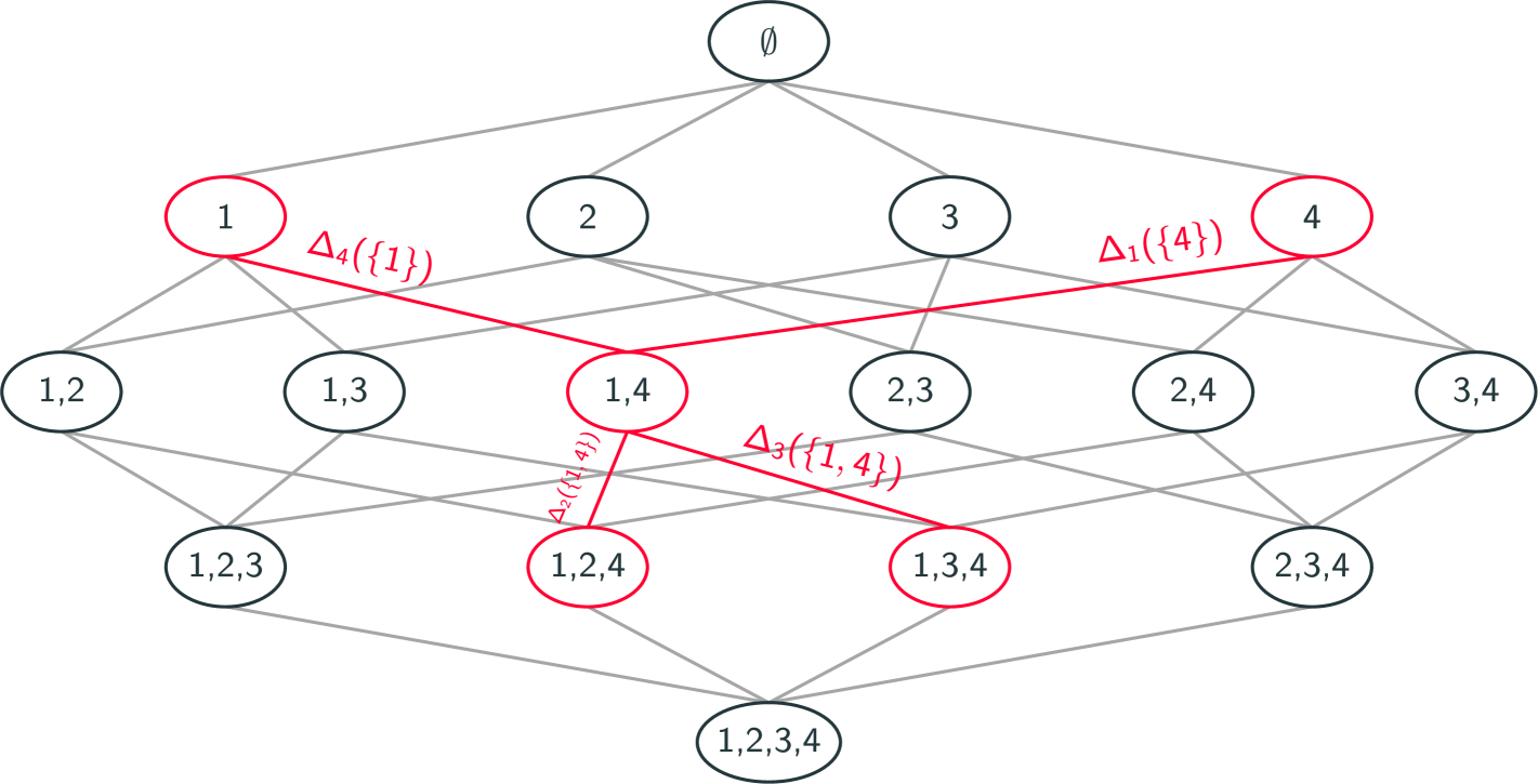
Figure 1: A cooperative game spans a lattice with each coalition $S\subseteq\mathcal{N}$ forming a node and each marginal contribution $\Delta_{i}(S)$ being represented by an edge between $S$ and $S\cup\{i\}$, exemplified here for $\mathcal{N}=\{1,2,3,4\}$. CMCS draws a random coalition $S$ and computes the extended marginal contributions $\Delta^{\prime}_{i}(S)=\Delta_{i}(S\setminus\{i\})$ of all players $i\in\mathcal{N}$. For $n=4$ it evaluates five coalitions and retrieves four marginal contributions.

5.1 Sampling Comparable Marginal Contributions

We start by observing that the sampling of marginal contributions can be designed to consume less than two evaluations of $\nu$ per sample. In fact, the budget restriction $T$ is not coupled to the evaluation of marginal contributions as atomic units but single accesses to $\nu$. Instead of separately evaluating $\nu(S)$ and $\nu(S\cup\{i\})$ for each $\Delta_{i}(S)$, the evaluations can be reused to form other marginal contributions and thus save budget. This idea can already be applied to the sampling of permutations of the player set. Castro et al. (2009) evaluate for each drawn permutation $\pi$ the marginal contribution $\Delta_{i}(\text{pre}_{i}(\pi))$ of each player $i$ to the preceding players in $\pi$. Except for the last player in $\pi$, each evaluation $\nu(\text{pre}_{i}(\pi)\cup\{i\})$ can be reused for the marginal contribution of the succeeding player.

We further develop this paradigm of sample reusage by exploiting the fact that any coalition $S\subseteq\mathcal{N}$ appears in $n$ many marginal contributions, one for each player, namely in $n-|S|$ many of the form $\Delta_{i}(S)$ for $i\notin S$ and $|S|$ many of the form $\Delta_{i}(S\setminus\{i\})$ for $i\in S$. We meaningfully unify both cases by establishing the notion of an extended marginal contribution in Definition 5.1.

Definition 5.1.

For any cooperative game $(\mathcal{N},\nu)$, the extended marginal contribution of a player $i\in\mathcal{N}$ to a coalition $S\subseteq\mathcal{N}$ is given by

$$\Delta^{\prime}_{i}(S):=\nu(S\cup\{i\})-\nu(S\setminus\{i\})\,.$$

Fittingly, this yields $\Delta_{i}^{\prime}(S)=\Delta_{i}(S\setminus\{i\})$ for $i\in S$ and $\Delta_{i}^{\prime}(S)=\Delta_{i}(S)=\Delta_{i}(S\setminus\{i\})$ for $i\notin S$. Thus, we circumvent the case of $\Delta_{i}(S)=0$ for $i\in S$.

We aim to draw in each round $m$ (of $M$ many) a coalition $S^{(m)}\subseteq\mathcal{N}$, compute the extended marginal contributions $\Delta^{\prime}_{i}(S^{(m)})$ of all players as illustrated in Figure 1, and update each $\hat{\phi}_{i}$ as the average of the corresponding observations:

$$\hat{\phi}_{i}=\frac{1}{M}\sum\limits_{m=1}^{M}\Delta^{\prime}_{i}\left(S^{(m)}\right)\,.$$ (13)

We reuse the coalition value $v_{S^{(m)}}=\nu(S^{(m)})$ to update all estimates by computing each extended marginal contribution as

$$\Delta^{\prime}_{i}\left(S^{(m)}\right)=\begin{cases}v_{S^{(m)}}-\nu(S^{(m)}\setminus\{i\})&\text{if }i\in S\\ \nu(S^{(m)}\cup\{i\})-v_{S^{(m)}}&\text{otherwise}\end{cases}\,.$$ (14)

Consequently, updating all $n$ estimates requires only $n+1$ calls to $\nu$ such that we obtain a budget-efficiency of $\frac{n}{n+1}$ sampled observations per call. In comparison, drawing marginal contributions separately yields a budget-efficiency of $\nicefrac{{1}}{{2}}$. In order to make this approach effective, it is desirable to obtain unbiased estimates leading to the question whether there even exists a probability distribution over $\mathcal{P}(\mathcal{N})$ to sample $S^{(m)}$ from such that $\mathbb{E}[\Delta^{\prime}_{i}(S^{(m)})]=\phi_{i}$ for all $i\in\mathcal{N}$. Indeed, we show its existence in Proposition 5.2 by means of a novel representation of the Shapley value based on extended marginal contributions.

Proposition 5.2.

For any cooperative game $(\mathcal{N},\nu)$, the Shapley value of each player $i\in\mathcal{N}$ is a weighted average of its extended marginal contributions. In particular, it holds

$$\phi_{i}=\sum\limits_{S\subseteq\mathcal{N}}\frac{1}{(n+1)\binom{n}{|S|}}\cdot\Delta^{\prime}_{i}(S)\,.$$

See Section A.2 for a proof. The weighted average allows to view the Shapley value as the expected extended marginal contribution and thus drawing $S^{(m)}$ from the distribution

$$\mathbb{P}\left(S^{(m)}=S\right)=\frac{1}{(n+1)\binom{n}{|S|}}\hskip 5.69046pt\text{for all }S\subseteq\mathcal{N}$$ (15)

yields unbiased estimates. Note that this is indeed a well-defined probability distribution over $\mathcal{P}(\mathcal{N})$ as shown in Section A.2. The resulting algorithm Comparable Marginal Contributions Sampling (CMCS) is given by Algorithm 1. It requires the cooperative game $(N,\nu)$, the budget $T$, and the parameter $k$ as input. The number of performed rounds $M$ is bounded by $M=\lfloor\frac{T}{n+1}\rfloor$. We solve sampling from the exponentially large power set of $\mathcal{N}$ by first drawing a size $\ell$ ranging from $0$ to $n$ uniformly at random (line 3) and then drawing uniformly a coalition $S$ of size $\ell$ (line 4). This results in the probability distribution of Equation 15 since there are $n+1$ sizes and $\binom{n}{\ell}$ coalitions of size $\ell$ to choose from. For the top-$k$ identification problem CMCS returns the set of $k$ many players $\hat{\mathcal{K}}$ for which it maintains the highest estimates $\hat{\phi}_{i}$. Ties are solved arbitrarily.

Algorithm 1 Comparable Marginal Contributions Sampling (CMCS)

Input: $(\mathcal{N},\nu)$, $T\in\mathbb{N},k\in[n]$

1: $\hat{\phi}_{i}\leftarrow 0$ for all $i\in\mathcal{N}$

2: for $m=1,\ldots,\lfloor\frac{T}{n+1}\rfloor$ do

3:  Draw $\ell\in\{0,\ldots,n\}$ uniformly at random

4:  Draw $S\subseteq\mathcal{N}$ with $|S|=\ell$ uniformly at random

5:  $v_{S}\leftarrow\nu(S)$

6:  for $i\in\mathcal{N}$ do

7:   $\Delta_{i}\leftarrow\begin{cases}v_{S}-\nu(S\setminus\{i\})&\text{if }i\in S\\ \nu(S\cup\{i\})-v_{S}&\text{otherwise}\end{cases}$

8:   $\hat{\phi}_{i}\leftarrow\frac{(m-1)\cdot\hat{\phi}_{i}+\Delta_{i}}{m}$

9:  end for

10: end for

Output: $\hat{\mathcal{K}}$ containing $k$ players with highest estimate $\hat{\phi}_{i}$

CMCS can also be applied for the approximate-all problem by simply returning its estimates since its sampling procedure and computation of estimates is independent of $k$. Thus, it is also an unbiased equifrequent player-wise independent sampler (see Section 4) because the marginal contributions obtained in each round stem from a fixed joint distribution and the resulting marginal distributions coincide with Equation 9 as implied by Proposition 5.2. Hence for $T$ being a multiple of $n+1$, its expected MSE is according to Equation 11:

$$\mathbb{E}[\text{MSE}]=\frac{n+1}{nT}\sum\limits_{i\in\mathcal{N}}\sigma_{i}^{2}\,.$$ (16)

For the top-$k$ identification the sampling scheme in CMCS yields an interesting property. All players share extended marginal contributions to the same reference coalitions $S^{(m)}$. Intuitively, this makes the estimates more comparable, as all have been updated using the same samples. Instead of estimating $\phi_{i}$ and $\phi_{j}$ precisely, CMCS answers the relevant question whether $\phi_{i}>\phi_{j}$ holds, by comparing the players marginal contributions to roughly the same coalitions, modulo the case of $i\in S$ and $j\notin S$ or vice versa. Instead, drawing marginal contributions separately, independently between the players, can, metaphorically speaking, be viewed as comparing apples with oranges.

Consequently, the estimates $\hat{\phi}_{i}$ and $\hat{\phi}_{j}$ are correlated and we further conjecture that the covariance $\text{Cov}(\Delta^{\prime}_{i}(S^{(m)}),\Delta^{\prime}_{j}(S^{(m)}))=\mathbb{E}[\Delta^{\prime}_{i}(S^{(m))}\Delta^{\prime}_{j}(S^{(m)})]-\mathbb{E}[\Delta^{\prime}_{i}(S^{(m)})]\mathbb{E}[\Delta^{\prime}_{j}(S^{(m)})]$ has a positive impact on the inclusion-exclusion error of CMCS in light of Theorem 4.1. For cooperative games in which the marginal contribution of a player is influenced by the coalitions size, our sampling scheme should yield positively correlated samples. In this case, if player $i$ or $j$ is added to the same coalition $S$, it is likely that both have a positive marginal contribution (or both share a negative) which in turn speaks for a positive covariance. For the general case, the covariance is stated in Proposition 5.3.

Proposition 5.3.

For any cooperative game $(\mathcal{N},\nu)$ the covariance between the extended marginal contributions of any players $i\neq j$ of the same round sampled by CMCS is given by

$$\text{Cov}\left(\Delta^{\prime}_{i}\left(S^{(m)}\right),\Delta^{\prime}_{j}\left(S^{(m)}\right)\right)=\frac{1}{n+1}\sum\limits_{S\subseteq\mathcal{N}\setminus\{i\}}\Delta_{i}(S)\\ \left(\frac{\Delta_{j}^{\prime}(S)}{\binom{n}{|S|}}+\frac{\Delta^{\prime}_{j}(S\cup\{i\})}{\binom{n}{|S|+1}}\right)-\phi_{i}\phi_{j}\,.$$

The proof is given in Section A.2. The sum can be seen as the Shapley value $\phi_{i}$ in which each marginal contribution of $i$ is additionally weighted by extended marginal contributions of $j$. To demonstrate the presumably positive covariance and give evidence to our conjecture, we consider a simple game of arbitrary size $n$ with $\nu(\mathcal{N})=1$ and $\nu(S)=0$ for all coalitions $S\neq\mathcal{N}$. Each player has a Shapley value of $\frac{1}{n}$ and the covariance in Proposition 5.3 given by $\frac{1}{n+1}-\frac{1}{n^{2}}$ is strictly positive for $n\geq 2$.

5.2 Relaxed Greedy Player Selection for Top-$k$ Identification

Striving for budget-efficiency in the design of a sample procedure might be favorable, however, CMCS as proposed in Section 5.1 is forced to spend budget on the retrieval of marginal contributions for all players in order to maximize budget-efficiency. This comes with the disadvantage that evaluations of $\nu$ are performed to sample for a player $i$ whose estimate $\hat{\phi}_{i}$ is possibly already reliable enough and does not need further updates compared to other players. This does not even require $\hat{\phi}_{i}$ to be precise in absolute terms. Instead, it is sufficient to predict with certainty whether $i$ belongs to the top-$k$ or not by comparing it to the other estimates. This observation calls for a more selective mechanism deciding which players to leave out in each round and thus save budget.

A radical approach is the greedy selection of a single player which maximizes a selection criterion based on the collected observations that incorporates incentives for exploration and exploitation. Gap-E (Gabillon et al., 2011; Bubeck et al., 2013) composes the selection criterion out of the uncertainty of a player’s top-$k$ (exploitation) membership and its number of observations (exploration). Similarly, BUS (Kolpaczki et al., 2021) selects the player $i$ minimizing the product of its estimate’s distance to the predicted top-$k$ border $\frac{1}{2}(\min_{i\in\hat{\mathcal{K}}}\hat{\phi}_{i}-\max_{j\in\mathcal{N}\setminus\hat{\mathcal{K}}}\hat{\phi}_{j})$ times its sample number $M_{i}$. In the same spirit but outside of the fixed-budget setting, SHAP$@$K (Kariyappa et al., 2024) chooses for given $\delta\in(0,1)$ the two players $i\in\hat{\mathcal{K}}$ and $j\in\mathcal{N}\setminus\hat{\mathcal{K}}$ with the highest overlap in their $\nicefrac{{\delta}}{{n}}$-confidence intervals of their estimates $\hat{\phi}_{i}$ and $\hat{\phi}_{j}$. It applies a stopping condition and terminates when no overlaps between $\hat{\mathcal{K}}$ and $\mathcal{N}\setminus\hat{\mathcal{K}}$ larger then a specified error $\varepsilon$ exist. Assuming normally distributed estimates $\hat{\phi}_{i}$ under the central limit theorem, it holds $\mathbb{P}(\rho_{\text{inc+exc}}(\hat{\mathcal{K}})\leq\varepsilon)\geq 1-\delta$ for its prediction $\mathcal{\hat{K}}$.

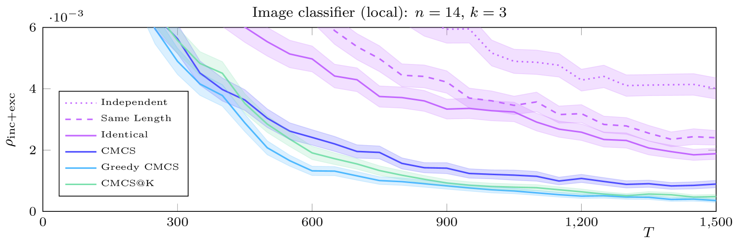
Figure 2: Inclusion-exclusion error $\varepsilon$ for increasingly comparable sampling variants (Independent, Same Length, Identical), incorporation of sample-reusage (CMCS), and greedy selection (Greedy CMCS, CMCS$@$K) depending on $T$.

Given the core idea of CMCS to draw samples for multiple players at once in order to increase budget-efficiency and obtain correlated observations, the greedy selection of a single player as done in (Gabillon et al., 2011; Kolpaczki et al., 2021) or just a pair (Kariyappa et al., 2024) is not suitable for our method. The phase-wise elimination performed by SAR (Bubeck et al., 2013) is not viable as it assumes all observations to be independent in order to analytically derive phase lengths. Instead, we relax the greediness by probabilistically selecting a set of players $P^{(m)}\subseteq\mathcal{N}$ in each round $m$, favoring those players who fulfill a selection criterion to higher degree. By doing so, we propose Greedy CMCS that intertwines the overcoming of the exploration-exploitation dilemma with the pursuit of budget-efficiency. We do not abandon exploration, since every player gets a chance to be picked, and the selection criterion incentivizes exploitation as it reflects how much the choice of a player benefits the prediction $\hat{\mathcal{K}}$.

Our selection criterion is based on the current knowledge of $\hat{\phi}_{1},\ldots,\hat{\phi}_{n}$ and the presumably best players $\hat{\mathcal{K}}$. Inspired by Theorem 4.1, we approximate the probability of each pair of players $i\in\hat{\mathcal{K}}$ and $j\in\mathcal{N}\setminus\hat{\mathcal{K}}$ being incorrectly partitioned by Greedy CMCS as

$$\hat{p}_{i,j}:=\Phi\left(\sqrt{M_{i,j}}\frac{\hat{\delta}_{i,j}}{\hat{\sigma}_{i,j}}\right)\,.$$ (17)

For all pairs $(i,j)\in\mathcal{N}^{2}$ we track:

• the number of times $M_{i,j}$ that both $i$ and $j$ have been selected in a round,

• the sampled marginal contributions’ mean difference $\hat{\delta}_{i,j}:=\frac{1}{M_{i,j}}\sum\limits_{m=1}^{M_{i,j}}\Delta^{\prime}_{j}(S^{(f_{i,j}(m))})-\Delta^{\prime}_{i}(S^{(f_{i,j}(m))})$ within these $M_{i,j}$ rounds, where $f_{i,j}(m)$ denotes the $m$-th round in which $i$ and $j$ are selected, and

• the estimate $\hat{\sigma}_{i,j}^{2}$ of the variance $\sigma_{i,j}^{2}:=\mathbb{V}[\Delta^{\prime}_{i}(S^{(m)})-\Delta^{\prime}_{j}(S^{(m)})]$ w.r.t. Equation 15.

Important to note is that we may not simply use the difference $\hat{\phi}_{j}-\hat{\phi}_{i}$ of our Shapley estimates, including all rounds, instead of $\hat{\delta}_{i,j}$ because $\hat{\phi}_{i}$ and $\hat{\phi}_{j}$ may differ in their respective total amount of total samples $M_{i}$ and $M_{j}$ such that the central limit theorem used for Theorem 4.1 is not applicable anymore. We derive Equation 17 in Section A.3.

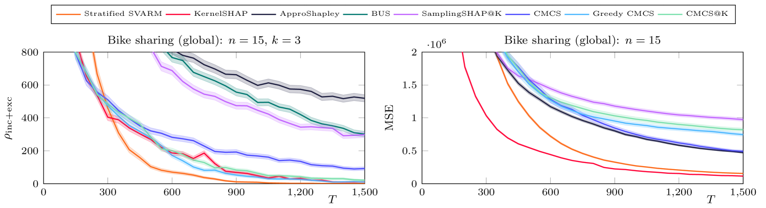
Figure 3: Comparison of achieved inclusion-exclusion error of various algorithms for top-$k$ identification (left) and approximate-all (right) depending on $T$.

For each pair $(i,j)\in\hat{\mathcal{K}}\times(\mathcal{N}\setminus\hat{\mathcal{K}})$ the estimate $\hat{p}_{i,j}$ quantifies how likely $i$ and $j$ are wrongly partitioned: Greedy CMCS estimates $\hat{\phi}_{i}\geq\hat{\phi}_{j}$ although $\phi_{i}<\phi_{j}$ holds. Since we want to minimize the probability of such a mistake, it comes natural to include the pair $(i,j)$ with the highest estimate $\hat{p}_{i,j}$ in the next round of Greedy CMCS to draw marginal contributions from, i.e. $i,j\in P^{(m)}$. As a consequence, $\hat{\phi}_{i}$ and $\hat{\phi}_{j}$ should become more reliable causing the error probability to shrink. Let $Q^{(m)}\subseteq\hat{\mathcal{K}}\times(\mathcal{N}\setminus\hat{\mathcal{K}})$ be the set of selected pairs in round $m$ from which the selected players are formed as $P^{(m)}=\{i\in\mathcal{N}\mid\exists(i,j)\in Q^{(m)}\lor\exists(j,i)\in Q^{(m)}\}$. In order to allow for more than two updated players in a round $m$, i.e. $|Q^{(m)}|>1$ , but waive pairs that are more likely to be correctly classified, we probabilistically include pairs in $Q^{(m)}$ depending on their $\hat{p}$-value. Let $\hat{p}_{\text{max}}=\max_{i\in\hat{\mathcal{K}},j\notin\hat{\mathcal{K}}}\hat{p}_{i,j}$ be the currently highest and $\hat{p}_{\text{min}}=\min_{i\in\hat{\mathcal{K}},j\notin\hat{\mathcal{K}}}\hat{p}_{i,j}$ the currently lowest value. We select each pair $(i,j)$ independently with probability

$$\mathbb{P}\left((i,j)\in Q^{(m)}\right)=\frac{\hat{p}_{i,j}-\hat{p}_{\text{min}}}{\hat{p}_{\text{max}}-\hat{p}_{\text{min}}}\hskip 5.69046pt\text{for all }(i,j)\in\hat{\mathcal{K}}\times(\mathcal{N}\setminus\hat{\mathcal{K}})\,.$$ (18)

This forces the pair with $\hat{p}_{\text{max}}$ to be picked and that with $\hat{p}_{\text{min}}$ to be left out. The probability of a pair beings elected increases monotonically with its $\hat{p}$-value.

Within an executed round we do not only collect marginal contributions for players in $P^{(m)}$ and update $M_{i,j}$, $\hat{\delta}_{i,j}$, and $\hat{\sigma}_{i,j}^{2}$ for all $(i,j)\in Q^{(m)}$. We use the collected information to its fullest by also updating the estimates of all pairs $(i,j)$ with both players being present in $P^{(m)}$ despite $(i,j)\notin Q^{(m)}$. Visually speaking, we update the complete subgraph induced by $P^{(m)}$ with players being nodes and edges containing the pairwise estimates.

Since the assumption of normally distributed estimates motivated by the central limit theorem is not appropriate for a low number of samples, we initialize Greedy CMCS with a warm-up phase as proposed for SHAP@K (Kariyappa et al., 2024). During the warm-up $M_{\text{min}}$ many rounds of CMCS are performed such that afterwards every player’s Shapley estimate is based on $M_{\text{min}}$ samples. This consumes a budget of $(n+1)M_{\text{min}}$ many evaluations. $M_{\min}$ is provided to Greedy CMCS as a parameter. Subsequently, the above described round-wise greedy sampling is applied as the second phase until the depletion of the in total available budget $T$. The pseudocode of the resulting algorithm Greedy CMCS is given in Appendix B.

Instead of our proposed selection mechanism, one can sample in the second phase only from the two players $i\in\hat{\mathcal{K}}$ and $j\notin\hat{\mathcal{K}}$ with the biggest overlap in confidence intervals as performed by SHAP@K. Leaving the sampling of CMCS in the first phase untouched, we call this variant CMCS$@$K. This is feasible since the choice of the sampling procedure in SHAP$@$K is to some extent arbitrary, as long as it yields confidence intervals for the Shapley estimates.

6 Empirical Results

We conduct multiple experiments of different designs to assess the performance of sampling comparable marginal contributions at the example of explanation tasks on real-world datasets. First, we demonstrate in Section 6.1 the iterative improvements of our proposed algorithmic tricks ranging from the naive independent sampling to Greedy CMCS and CMCS$@$K. Section 6.2 investigates whether favorable MSE values of algorithms for the approximate-all problem translate on the same cooperative games to the inclusion-exclusion error for top-$k$ identification. In Section 6.3 we compare our variants of CMCS against baselines and state-of-the-art competitors. Lastly, we investigate in Section 6.4 the required budget until the stopping criterion of (Kariyappa et al., 2024) applied to CMCS guarantees an error of at most $\varepsilon$ with probability at least $1-\delta$.

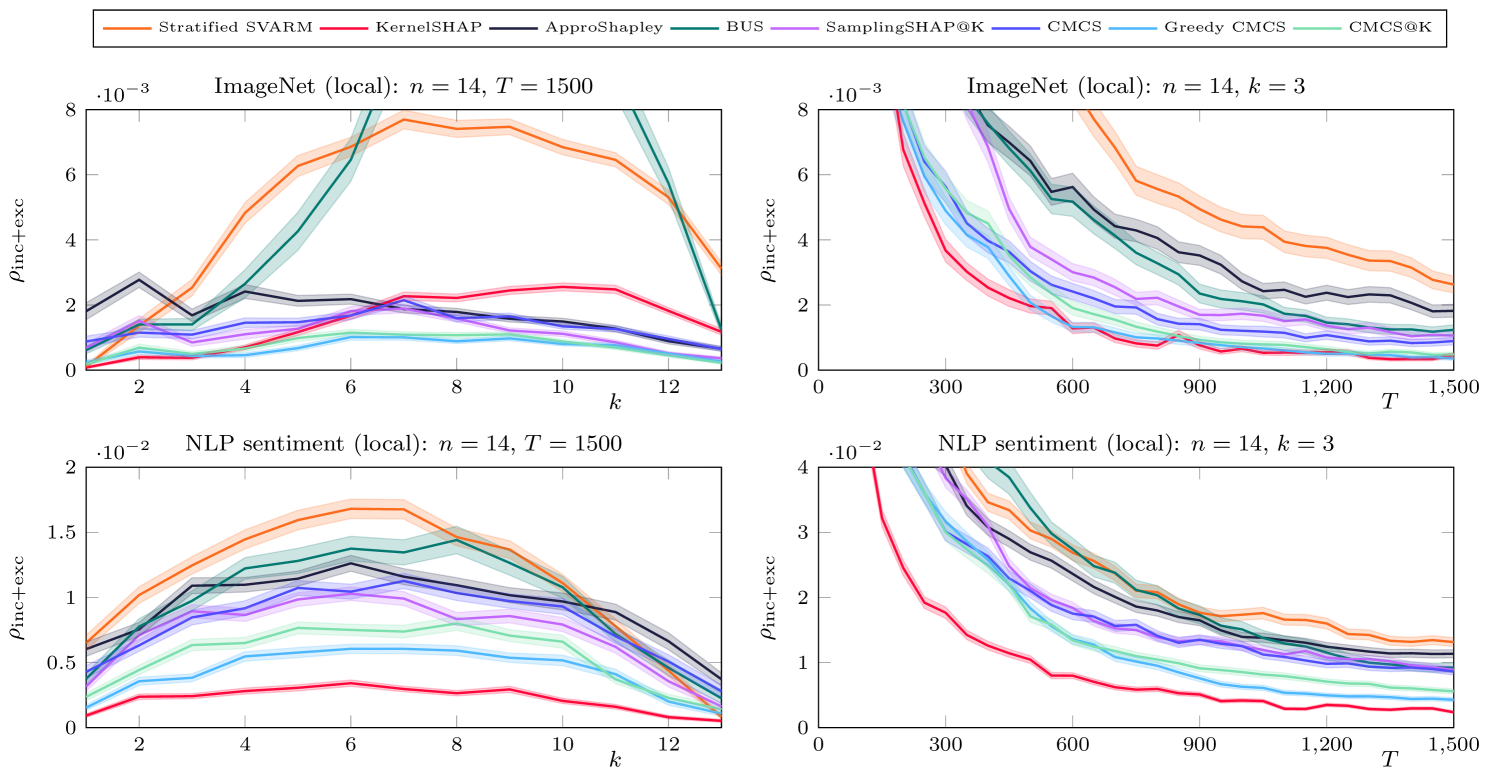
Figure 4: Comparison of achieved inclusion-exclusion error with baselines for local explanations: fixed budget with varying $k$ (left) and fixed $k$ with increasing budget (right).

All performance measures are calculated by exhaustively computing the Shapley values in advance and averaging the results over 1000 runs. Standard errors are included as shaded bands. We compare against ApproShapley (Castro et al., 2009), KernelSHAP (Lundberg & Lee, 2017) (with reference implementation provided by the shap python package, the one to sample without replacement), Stratified SVARM (Kolpaczki et al., 2024a), BUS (Kolpaczki et al., 2021), and SamplingSHAP$@$K (Kariyappa et al., 2024) which is SHAP@K drawing samples according to ApproShapley. For both SamplingSHAP$@$K and CMCS$@$K, we use $M_{\text{min}}=30$ and confidence intervals of $\nicefrac{{\delta}}{{n}}$ with $\delta=0.001$. We drop Gap-E (Gabillon et al., 2011) and SAR (Bubeck et al., 2013) due to worse performances .

Datasets and games.

Analogously to (Kolpaczki et al., 2024a, b), we generate cooperative games from two types of explanation tasks in which the Shapley values represent feature importance scores. For global games, we construct the value function by training a sklearn random forest with 20 trees on each feature subset and taking its classification accuracy, or the $R^{2}$-metric for regression tasks, on a test set as the coalitions’ worth. We employ the Adult ($n=14$, classification), Bank Marketing ($n=16$, classification), Bike Sharing ($n=15$, regression), Diabetes ($n=10$, regression), German Credit ($n=20$, classification), Titanic ($n=11$, classification), and Wine ($n=13$, classification) dataset. For local games, we create a game by picking a random datapoint and taking a pretrained model’s prediction value as each coalition’s worth. Feature values are imputed by their mean, respectively mode. For this purpose we take the Adult ($n=14$, XGBoost, classification), ImageNet ($n=14$, ResNet18, classification), and NLP Sentiment ($n=14$, DistilBERT transformer, regression, IMDB data) dataset.

6.1 Advantage of Comparable Sampling

Greedy CMCS builds upon multiple ideas whose effects onto the approximation quality is depicted in isolation by Figure 2. As a baseline we consider the independent sampling of marginal contributions of each player with distribution given in Equation 9. The comparability of the samples is stepwise increased by sampling in each round marginal contributions to coalitions of the same length for all players, and next using the identical coalition $S^{(m)}$ drawn according to Equation 15. In compliance with our conjecture, the decreasing error from independent to same length and further to identical speaks in favor of the beneficial impact that comes with correlated observations. The biggest leap in performance is caused by reusing the evaluated worth $\nu(S^{(m)})$ appearing in each marginal contribution of the independent variant resulting in CMCS. The sample reusage alone almost doubles the budget-efficiency from $\nicefrac{{1}}{{2}}$ to $\nicefrac{{n}}{{n+1}}$. On top of that, incorporating (relaxed) greedy sampling gifts Greedy CMCS and CMCS@K a further advantage by halving the error for higher budget ranges.

6.2 MSE vs. Inclusion-Exclusion Error

Given the similarities between the problem statements of approximating all Shapley values (cf. Section 3.2) and that of top-$k$ identification (cf. Section 3.3) at first sight, one might suspect that approximation algorithms performing well in the former, also do so in the latter and vice versa. However, Figure 3 shows a different picture. The best performing methods Stratified SVARM and KernelSHAP remain consistent but change in order. The variants of CMCS are less favorable in terms of MSE but are barely outperformed in top-$k$ identification. We interpret this as further evidence that top-$k$ identification indeed rewards positively correlated samples supporting our intuition of comparability. Most striking is the difference between ApproShapley and CMCS. Assuming to know $\nu(\emptyset)=0$, ApproShapley exhibits a budget-efficiency of $1$ as it consumes in each sampled permutation $n$ evaluations and retrieves $n$ marginal contributions, which is only slightly better than that of CMCS with $\nicefrac{{n}}{{n+1}}$. Thus, it should be only marginally better in approximation according to Equation 11 and Equation 16. Our results in Figure 3 confirm the precision of our theory. However, notice how CMCS significantly outperforms ApproShapley in terms of $\rho_{\text{inc+exc}}$ despite the almost identical budget usage. Hence, it is the stronger correlation of samples drawn by CMCS combined with the nature of top-$k$ identification that causes the observed advantage of comparable sampling.

6.3 Comparison with Existing Methods

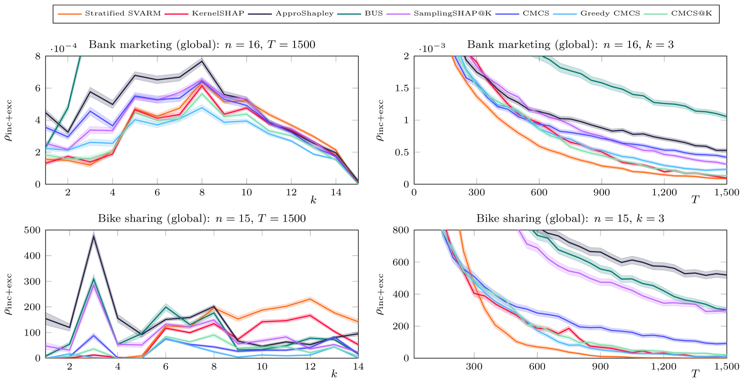
Figure 5: Comparison of achieved inclusion-exclusion error with baselines for global explanations: fixed budget with varying $k$ (left) and fixed $k$ with increasing budget (right).

Figure 4 and 5 compare the performances of our methods against baselines for local and global games. For fixed $k=3$, we observe the competitiveness of Greedy CMCS and CMCS$@$K being mostly on par with KernelSHAP, but getting beaten by Stratified SVARM for global games, which in turns subsides at local games. Greedy CMCS exhibits stable performance across both explanation types and the whole range of $k$. On the other hand, if instead the budget is fixed, Greedy CMCS has often the upper hand for values of $k$ close to $\nicefrac{{n}}{{2}}$ and is even with KernelSHAP for lower $k$.

6.4 Budget Consumption for PAC Solution

Assuming normally distributed Shapley estimates, SHAP$@$K is a $(\varepsilon,\delta)$-PAC learner (Kariyappa et al., 2024), i.e. upon self-induced termination it holds $\rho_{\text{inc+exc}}(\hat{\mathcal{K}})\leq\varepsilon$ with probability at least $1-\delta$. KernelSHAP is not applicable as it does not yield confidence bounds. For this reason Kariyappa et al. (2024) sample marginal contributions referred as SamplingSHAP$@$K. Its stopping condition is triggered as soon as no $\nicefrac{{\delta}}{{n}}$ confidence intervals for the estimates $\hat{\phi}_{i}$ overlap between $\hat{\mathcal{K}}$ and $\mathcal{N}\setminus\hat{\mathcal{K}}$. We apply the stopping condition to our algorithms and compare to SamplingSHAP$@$K in the PAC-setting. Table 1 shows the average number of calls to $\nu$ until termination that is to be minimized. For some local games the number of calls is significantly higher due to the large variance in the difficulty of the respective games induced from each datapoint. CMCS$@$K shows the best results in nearly every game by some margin, which makes it the algorithm of choice for PAC-learning. Thus, CMCS@K is preferable when guarantees for approximation quality are required and improves upon SHAP$@$K due to its refined sampling mechanism.

		SamplingSHAP@K		CMCS		CMCS@K		Greedy CMCS
Game	$n$	#samples	SE	#samples	SE	#samples	SE	#samples	SE
Adult (global)	14	38 998	1 247	137 861	2 517	30 995	673	39 071	738
German credit (global)	20	21 939	336	56 738	1 129	16 437	248	22 327	328
Bike sharing (global)	15	4 850	97	13 053	164	3 982	54	8 894	117
Bank marketing (global)	16	15 124	287	39 144	875	12 000	206	16 260	267
Diabetes (global)	10	3 723	94	7 793	143	2 976	55	4 593	85
Titanic (global)	11	4 852	113	11 036	237	3 884	72	5 782	124
Wine (global)	13	34 953	1 046	120 859	1 906	29 913	641	34 265	501
NLP sentiment (local)	14	626 346	188 125	3 351 274	764 663	568 261	156 674	447 252	77 149
ImageNet (local)	14	135 851	39 335	578 670	196 181	108 267	32 067	261 586	147 126
Adult (local)	14	18 464	4 391	55 779	17 954	14 406	3 645	16 160	3 765

Table 1: Average number of calls to $\nu$ in the PAC-setting (see Equation 8) across different datasets averaged over 200 runs using $\delta=0.01$ and $\epsilon=0.0005$ for $k=5$.

7 Conclusion

We emphasized differences between the problem of approximating all Shapley values and that of identifying the $k$ players with highest Shapley values. Analytically recognizing the advantage that correlated samples promise, we developed with CMCS an antithetic sampling algorithm that reuses evaluations to save budget. Our extensions Greedy CMCS and CMCS$@$K employ selective strategies for sampling. Both demonstrate competitive performances, with Greedy CMCS being better suited for fixed budgets, whereas CMCS$@$K is clearly favorable in the PAC-setting. Our proposed methods are not only model-agnostic, moreover, they can handle any cooperative game, facilitating their application for any explanation type and domain even outside of explainable AI. The difficulties that some algorithms face when translating their performance to top-$k$ identification suggest that practitioner’s being consciously interested in top-$k$ explanations might have an advantage by applying tailored top-$k$ algorithms instead of the trivial reduction to the approximate-all problem. Future work could investigate the sensible choice of the warm-up length in Greedy CMCS and CMCS$@$K which poses a trade-off between exploration and exploitation. Modifying our considered problem statement to identify the players with highest absolute Shapley values poses an intriguing variation for detecting the most impactful players and opens the door to new approaches. Finally, Shapley interactions enrich Shapley-based explanations. The number of pairwise interactions grows quadratically with $n$, hence top-$k$ identification could play an even more significant role. Our work can be understood as a methodological precursor to such extensions.

Appendix A Theoretical Analysis

A.1 Proof of Theorem 4.1

For the estimate $\hat{\mathcal{K}}\subseteq\mathcal{N}$ returned by an algorithm for the top-$k$ identification problem we can obviously state

$$\begin{array}[]{l}\mathbb{P}(\hat{\mathcal{K}}\in\mathbb{K}_{\varepsilon})=\sum\limits_{\mathcal{K}\in\mathbb{K}_{\varepsilon}}\mathbb{P}(\hat{\mathcal{K}}=\mathcal{K})\,.\end{array}$$

Given the construction of $\hat{\mathcal{K}}$, $\mathcal{A}$ must choose any $i\in\mathcal{N}$ to be in $\hat{\mathcal{K}}$ if $\hat{\phi}_{i}>\hat{\phi}_{j}$ holds for at least $n-k$ many players $j\in\mathcal{N}$. Hence, for any $\mathcal{K}\in\mathbb{K}_{\varepsilon}$ we have:

$$\begin{array}[]{rl}\mathbb{P}(\hat{\mathcal{K}}=\mathcal{K})\geq&\ \mathbb{P}(\forall i\in\mathcal{K}\ \forall j\in\mathcal{N}\setminus\mathcal{K}:\hat{\phi}_{i}>\hat{\phi}_{j})\\ =&\ 1-\mathbb{P}(\exists i\in\mathcal{K}\ \exists j\in\mathcal{N}\setminus\mathcal{K}:\hat{\phi}_{i}\leq\hat{\phi}_{j})\\ \geq&\ 1-\sum\limits_{\begin{subarray}{c}i\in\mathcal{K}\\ j\in\mathcal{N}\setminus\mathcal{K}\end{subarray}}\mathbb{P}(\hat{\phi}_{i}\leq\hat{\phi}_{j})\end{array}$$

Given the assumptions on the sampling procedure and the aggregation to estimates $\hat{\phi}_{1},\ldots,\hat{\phi}_{n}$, we can apply the central limit theorem (CLT) to state that for any $i\in\mathcal{K}$ and $j\in\mathcal{N}\setminus\mathcal{K}$ the distribution of $\sqrt{M}\left((\hat{\phi}_{i}-\hat{\phi}_{j})-(\phi_{i}-\phi_{j})\right)$ converges to a normal distribution with mean $0$ and variance $\sigma_{i,j}^{2}$ as $M\to\infty$ since $\mathbb{E}[\hat{\phi}_{i}-\hat{\phi}_{j}]=\phi_{i}-\phi_{j}$. Although $M$ is finite as it is limited by the budget $T$, we assume it to be normally distributed, to which it comes close to in practice for large $M$. Hence, for any $i\in\mathcal{K}$ and $j\in\mathcal{N}\setminus\mathcal{K}$ we derive:

$$\begin{array}[]{rl}\mathbb{P}(\hat{\phi}_{i}\leq\hat{\phi}_{j})=&\ \mathbb{P}(\hat{\phi}_{i}-\hat{\phi}_{j}\leq 0)\\ =&\ \mathbb{P}((\hat{\phi}_{i}-\hat{\phi}_{j})-(\phi_{i}-\phi_{j})\leq-(\phi_{i}-\phi_{j}))\\ =&\ \mathbb{P}(\sqrt{M}((\hat{\phi}_{i}-\hat{\phi}_{j})-(\phi_{i}-\phi_{j}))\leq\sqrt{M}(\phi_{j}-\phi_{i}))\\ \stackrel{{\scriptstyle CLT}}{{=}}&\ \Phi\left(\sqrt{M}\frac{\phi_{j}-\phi_{i}}{\sigma_{i,j}}\right)\end{array}$$

where $\Phi$ is the standard normal cumulative distribution function. Putting the intermediate results together, we obtain

$$\begin{array}[]{l}\mathbb{P}(\hat{\mathcal{K}}\in\mathbb{K}_{\varepsilon})\geq\sum\limits_{\mathcal{K}\in\mathbb{K}_{\epsilon}}\left[1-\sum\limits_{\begin{subarray}{c}i\in\mathcal{K}\\ j\in\mathcal{N}\setminus\mathcal{K}\end{subarray}}\Phi\left(\sqrt{M}\frac{\phi_{j}-\phi_{i}}{\sigma_{i,j}}\right)\right]\,.\end{array}$$

A.2 Comparable Marginal Contributions Sampling

Proof that Equation 15 induces a well-defined probability distribution:
Obviously it holds $\mathbb{P}(S)\geq 0$ and for the sum of probabilities we have:

$$\begin{array}[]{l}\sum\limits_{S\subseteq\mathcal{N}}\mathbb{P}(S)=\sum\limits_{S\subseteq\mathcal{N}}\frac{1}{(n+1)\binom{n}{|S|}}=\sum\limits_{\ell=0}^{n}\sum\limits_{\begin{subarray}{c}S\subseteq\mathcal{N}\\ |S|=l\end{subarray}}\frac{1}{(n+1)\binom{n}{\ell}}=\sum\limits_{\ell=0}^{n}\frac{\binom{n}{\ell}}{(n+1)\binom{n}{\ell}}=1\,.\end{array}$$

Proof of Proposition 5.2:
For any $i\in\mathcal{N}$ we derive:

$$\begin{array}[]{rl}\sum\limits_{S\subseteq\mathcal{N}}\frac{1}{(n+1)\binom{n}{|S|}}\cdot\Delta^{\prime}_{i}(S)=&\ \sum\limits_{\begin{subarray}{c}S\subseteq\mathcal{N}\\ i\in S\end{subarray}}\frac{1}{(n+1)\binom{n}{|S|}}\cdot\Delta_{i}(S\setminus\{i\})+\sum\limits_{\begin{subarray}{c}S\subseteq\mathcal{N}\\ i\notin S\end{subarray}}\frac{1}{(n+1)\binom{n}{|S|}}\cdot\Delta_{i}(S)\\ =&\ \sum\limits_{S\subseteq\mathcal{N}\setminus\{i\}}\frac{1}{(n+1)\binom{n}{|S|+1}}\cdot\Delta_{i}(S)+\sum\limits_{S\subseteq\mathcal{N}\setminus\{i\}}\frac{1}{(n+1)\binom{n}{|S|}}\cdot\Delta_{i}(S)\\ =&\ \sum\limits_{S\subseteq\mathcal{N}\setminus\{i\}}\frac{1}{n+1}\left(\frac{1}{\binom{n}{|S|+1}}+\frac{1}{\binom{n}{|S|}}\right)\cdot\Delta_{i}(S)\\ =&\ \sum\limits_{S\subseteq\mathcal{N}\setminus\{i\}}\frac{1}{n\cdot\binom{n-1}{|S|}}\cdot\Delta_{i}(S)\\ =&\ \phi_{i}\end{array}$$

Proof of Proposition 5.3:
Given the unbiasedness of the samples, i.e. $\mathbb{E}[\Delta^{\prime}_{i}(S^{(m)})]=\phi_{i}$ for every $i\in\mathcal{N}$, the covariance is given by:

$$\begin{array}[]{rl}\text{Cov}\left(\Delta^{\prime}_{i}(S^{(m)}),\Delta^{\prime}_{j}(S^{(m)})\right)=&\ \mathbb{E}\left[\Delta^{\prime}_{i}(S^{(m)})\Delta^{\prime}_{j}(S^{(m)})\right]-\mathbb{E}\left[\Delta^{\prime}_{i}(S^{(m)})\right]\mathbb{E}\left[\Delta^{\prime}_{j}(S^{(m)})\right]\\ =&\ \mathbb{E}\left[\Delta^{\prime}_{i}(S^{(m)})\Delta^{\prime}_{j}(S^{(m)})\right]-\phi_{i}\phi_{j}\\ \end{array}$$

For the first term we derive:

$$\begin{array}[]{rl}&\ \mathbb{E}\left[\Delta^{\prime}_{i}(S^{(m)})\Delta^{\prime}_{j}(S^{(m)})\right]\\ =&\ \sum\limits_{S\subseteq\mathcal{N}}\frac{1}{(n+1)\binom{n}{|S|}}\cdot\Delta^{\prime}_{i}(S)\Delta^{\prime}_{j}(S)\\ =&\ \frac{1}{n+1}\sum\limits_{S\subseteq\mathcal{N}\setminus\{i,j\}}\frac{\Delta_{i}(S)\Delta_{j}(S)}{\binom{n}{|S|}}+\frac{\Delta_{i}(S)\Delta_{j}(S\cup\{i\})}{\binom{n}{|S|+1}}+\frac{\Delta_{i}(S\cup\{j\})\Delta_{j}(S)}{\binom{n}{|S|+1}}+\frac{\Delta_{i}(S\cup\{j\})\Delta_{j}(S\cup\{i\})}{\binom{n}{|S|+2}}\\ =&\ \frac{1}{n+1}\sum\limits_{S\subseteq\mathcal{N}\setminus\{i,j\}}\Delta_{i}(S)\cdot\left(\frac{\Delta_{j}(S)}{\binom{n}{|S|}}+\frac{\Delta_{j}(S\cup\{i\})}{\binom{n}{|S|+1}}\right)+\Delta_{i}(S\cup\{j\})\cdot\left(\frac{\Delta_{j}(S)}{\binom{n}{|S|+1}}+\frac{\Delta_{j}(S\cup\{i\})}{\binom{n}{|S|+2}}\right)\\ =&\ \frac{1}{n+1}\sum\limits_{S\subseteq\mathcal{N}\setminus\{i\}}\Delta_{i}(S)\cdot\left(\frac{\Delta_{j}^{\prime}(S)}{\binom{n}{|S|}}+\frac{\Delta^{\prime}_{j}(S\cup\{i\})}{\binom{n}{|S|+1}}\right)\end{array}$$

A.3 Approximating Pairwise Probabilities for Greedy CMCS

Analogously to Section A.1, we derive for any pair $i,j\in\mathcal{N}$ and unbiased equifrequent player-wise independent sampler:

$$\begin{array}[]{rl}\mathbb{P}(\phi_{i}<\phi_{j})=&\ \mathbb{P}(\phi_{i}-\phi_{j}<0)\\ =&\ \mathbb{P}((\hat{\phi}_{i}-\hat{\phi}_{j})-(\phi_{i}-\phi_{j})>\hat{\phi}_{i}-\hat{\phi}_{j})\\ =&\ \mathbb{P}(\sqrt{M}((\hat{\phi}_{i}-\hat{\phi}_{j})-(\phi_{i}-\phi_{j}))>\sqrt{M}(\hat{\phi}_{i}-\hat{\phi}_{j}))\\ \stackrel{{\scriptstyle CLT}}{{=}}&\ \Phi\left(\sqrt{M}\frac{\hat{\phi}_{j}-\hat{\phi}_{i}}{\sigma_{i,j}}\right)\end{array}$$

Since this statement does not require the knowledge of an eligible coalition $\mathcal{K}$, we can estimate the likelihood of $\phi_{i}<\phi_{j}$ during runtime of the approximation algorithm. For this purpose, we use the sample variance to estimate $\sigma_{i,j}$. Note that $M$ is the number of drawn samples that both $\hat{\phi}_{i}$ and $\hat{\phi}_{j}$ share. Since the players’ marginal contributions are selectively sampled, Greedy CMCS substitutes $M$ by the true number of joint appearances $M_{i,j}$ and $\hat{\phi}_{i}-\hat{\phi}_{j}$ by $\hat{\delta}_{i,j}$ which only takes into account marginal contributions of $i$ and $j$ which have been acquired during rounds in which both players have been selected.

Appendix B Pseudocode of Greedy CMCS

In addition to the pseudocode in Algorithm 2, we provide further details regarding the tracking of estimates and probabilistic selection of players.

Algorithm 2 Greedy CMCS

Input: $(\mathcal{N},\nu)$, $T\in\mathbb{N},k\in[n],M_{\text{min}}$

1: $\hat{\phi}_{i},M_{i}\leftarrow 0$ for all $i\in\mathcal{N}$

2: $M_{i,j},\Sigma_{i,j},\Gamma_{i,j}\leftarrow 0$ for all $i,j\in\mathcal{N}$

3: $t\leftarrow 0$

4: while $t<T$ do

5:  Draw $\ell\in\{0,\ldots,n\}$ uniformly at random

6:  Draw $S\subseteq\mathcal{N}$ with $|S|=l$ uniformly at random

7:  $v_{S}\leftarrow\nu(S)$

8:  $t\leftarrow t+1$

9:  $P\leftarrow\textsc{{SelectPlayers}}$

10:  for $i\in P$ do

11:   if $t=T$ then

12:    exit

13:   end if

14:   $\Delta_{i}\leftarrow\begin{cases}v_{S}-\nu(S\setminus\{i\})&\text{if }i\in S\\ \nu(S\cup\{i\})-v_{S}&\text{otherwise}\end{cases}$

15:   $\hat{\phi}_{i}\leftarrow\frac{(M_{i}-1)\cdot\hat{\phi}_{i}+\Delta_{i}}{M_{i}}$

16:   $M_{i}\leftarrow M_{i}+1$

17:   $t\leftarrow t+1$

18:  end for

19:  $M_{i,j}\leftarrow M_{i,j}+1$ for all $i,j\in P$

20:  $\Sigma_{i,j}\leftarrow\Sigma_{i,j}+(\Delta_{i}-\Delta_{j})$ for all $i,j\in P$

21:  $\Gamma_{i,j}\leftarrow\Gamma_{i,j}+(\Delta_{i}-\Delta_{j})^{2}$ for all $i,j\in P$

22: end while

Output: $\hat{\mathcal{K}}$ containing $k$ players with highest estimate $\hat{\phi}_{i}$

• Initialize estimator $\hat{\phi}_{i}$ and individual counter of sampled marginal contributions $M_{i}$ for each player.

• Initialize for each player pair: the counter for joint appearances in rounds $M_{i,j}$, the sum of differences of marginal contributions $\Sigma_{i,j}$, and the sum of squared differences of marginal contributions $\Gamma_{i,j}$.

• Given $d_{m}:=\Delta_{i}(S_{m}\setminus\{i\})-\Delta_{j}(S_{m}\setminus\{j\})$ the unbiased variance estimator is

  $$\begin{array}[]{l}\hat{\sigma}_{i,j}^{2}:=\frac{1}{M_{i,j}-1}\sum\limits_{m=1}^{M_{i,j}}(d_{m}-\bar{d})^{2}=\frac{1}{M_{i,j}-1}\left(\Gamma_{i,j}-\frac{\Sigma_{i,j}^{2}}{M_{i,j}}\right)\,.\end{array}$$

• In each round, select with SelectPlayers players $P$ for whom to form an extended marginal contribution:

  • First phase: select all players $M_{\text{min}}$ times: $P=\mathcal{N}$.

  • Second phase: otherwise, partition the players into top-$k$ players $\hat{\mathcal{K}}$ and the rest $\hat{\mathcal{K}}^{\prime}=\mathcal{N}\setminus\hat{\mathcal{K}}$ based on the estimates $\hat{\phi}_{1},\ldots,\hat{\phi}_{n}$.

  • Compute $\hat{p}_{i,j}\approx P(\phi_{i}<\phi_{j})$ for all pairs $i\in\hat{\mathcal{K}},j\in\hat{\mathcal{K}}^{\prime}$.

  • If all pairs are equally probable, select all players as it is not reasonable to be selective.

  • Otherwise, sample a set of pairs $Q$ based on $\hat{p}_{i,j}$.

  • Select all players as members of $P$ that are in at least one pair in $Q$.

• Sample a coalition $S$ and cache its value.

• Form for all selected players in $P$ their extended marginal contribution $\Delta_{i}^{\prime}(S)$ and update their estimator $\hat{\phi}_{i}$.

• Update the values $M_{i,j}$, $\Sigma_{i,j}$, and $\Gamma_{i,j}$ for all $i,j\in P$ required for computing the variance estimates $\hat{\sigma}_{i,j}^{2}$ and $\hat{p}_{i,j}$.

• In practice, we precompute and cache $\nu(\emptyset)$ and $\nu(\mathcal{N})$ in the beginning. We do that for ALL tested algorithms for a fair comparison.

• We modify Stratified SVARM to only precompute coalition values for sizes $0$ and $n$, instead of including sizes $1$ and $n-1$. Instead of integrating this optimization into all our algorithms, we remove it as it requires a budget of $2n$ which might be infeasible for games with large numbers of players.

Algorithm 3 SelectPlayers

1: $P\leftarrow\mathcal{N}$

2: if $M_{i,j}\geq M_{\text{min}}$ for all $i,j\in\mathcal{N}$ then

3:  $\hat{\mathcal{K}}\leftarrow$ $k$ players of $\mathcal{N}$ with highest estimate $\hat{\phi}_{i}$, solve ties arbitrarily

4:  $\hat{\mathcal{K}}^{\prime}\leftarrow\mathcal{N}\setminus\hat{\mathcal{K}}$

5:  $\hat{\sigma}^{2}_{i,j}\leftarrow\frac{1}{M_{i,j}-1}\left(\Gamma_{i,j}-\frac{\Sigma_{i,j}^{2}}{M_{i,j}}\right)$ for all $i\in\hat{\mathcal{K}},j\in\hat{\mathcal{K}}^{\prime}$

6:  $\hat{p}_{i,j}\leftarrow\Phi\left(\sqrt{M_{i,j}}\frac{-\Sigma_{i,j}}{\sqrt{\hat{\sigma}^{2}_{i,j}}}\right)$ for all $i\in\hat{\mathcal{K}},j\in\hat{\mathcal{K}}^{\prime}$

7:  if $\min_{i,j}\hat{p}_{i,j}\neq\max_{i,j}\hat{p}_{i,j}$ then

8:   $P,Q\leftarrow\emptyset$

9:   for $(i,j)\in\hat{\mathcal{K}}\times\hat{\mathcal{K}}^{\prime}$ do

10:    Draw Bernoulli realization $B_{i,j}$ with $\mathbb{P}(B_{i,j}=1)=\frac{\hat{p}_{i,j}-\min_{i,j}\hat{p}_{i,j}}{\max_{i,j}\hat{p}_{i,j}-\min_{i,j}\hat{p}_{i,j}}$

11:    if $B_{i,j}=1$ then

12:     $Q\leftarrow Q\cup\{(i,j)\}$

13:     $P\leftarrow P\cup\{i,j\}$

14:    end if

15:   end for

16:  end if

17: end if

Output: $\mathcal{P}$

Appendix C Further Empirical Results

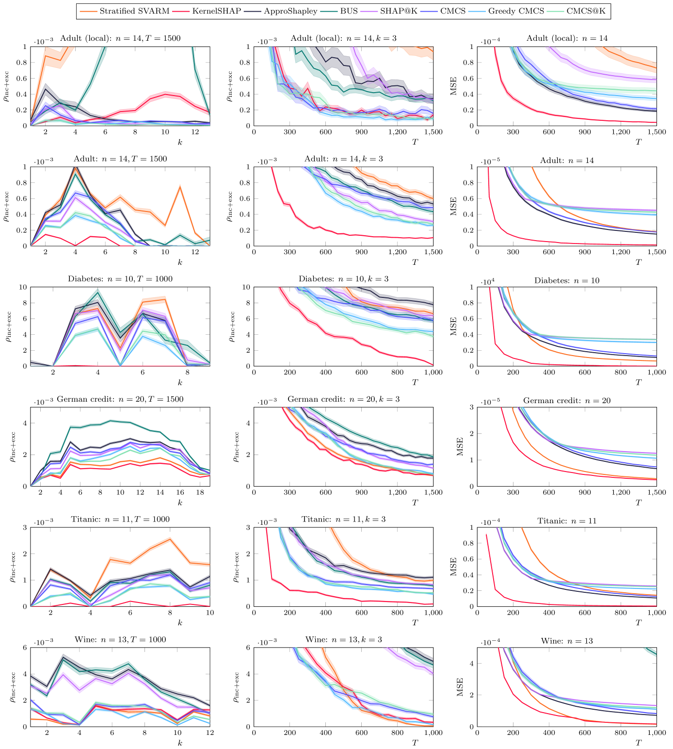
Figure 6: Comparison of achieved error with baselines: inclusion-exclusion error for fixed budget with varying $k$ (left), inclusion-exclusion error for fixed $k$ with increasing budget (middle), and MSE depending on budget (right).

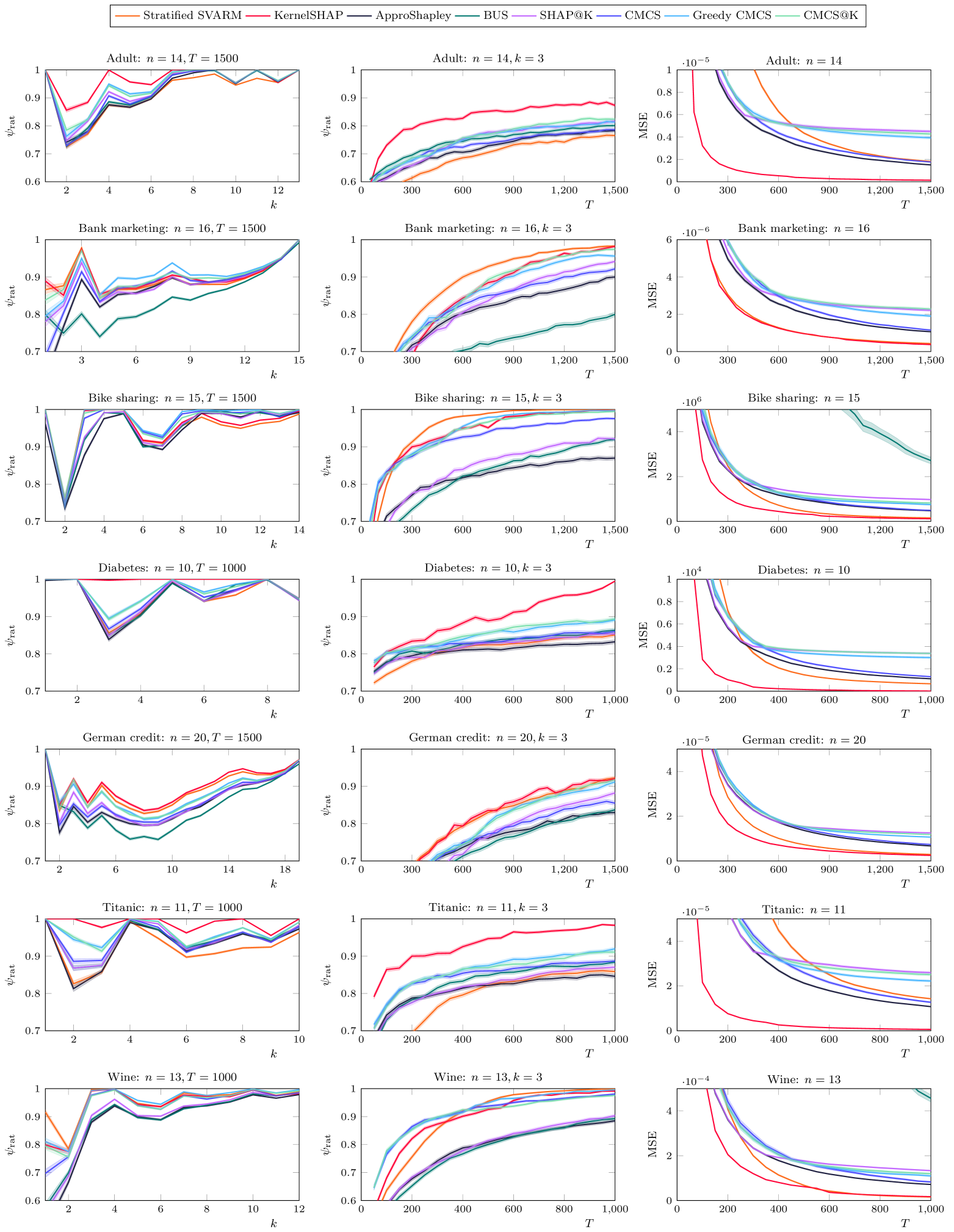
Figure 7: Comparison of achieved ratio precision and MSE with baselines for global explanations: precision for fixed budget with varying $k$ (left), precision for fixed $k$ with increasing budget (middle), and MSE depending on budget (right).

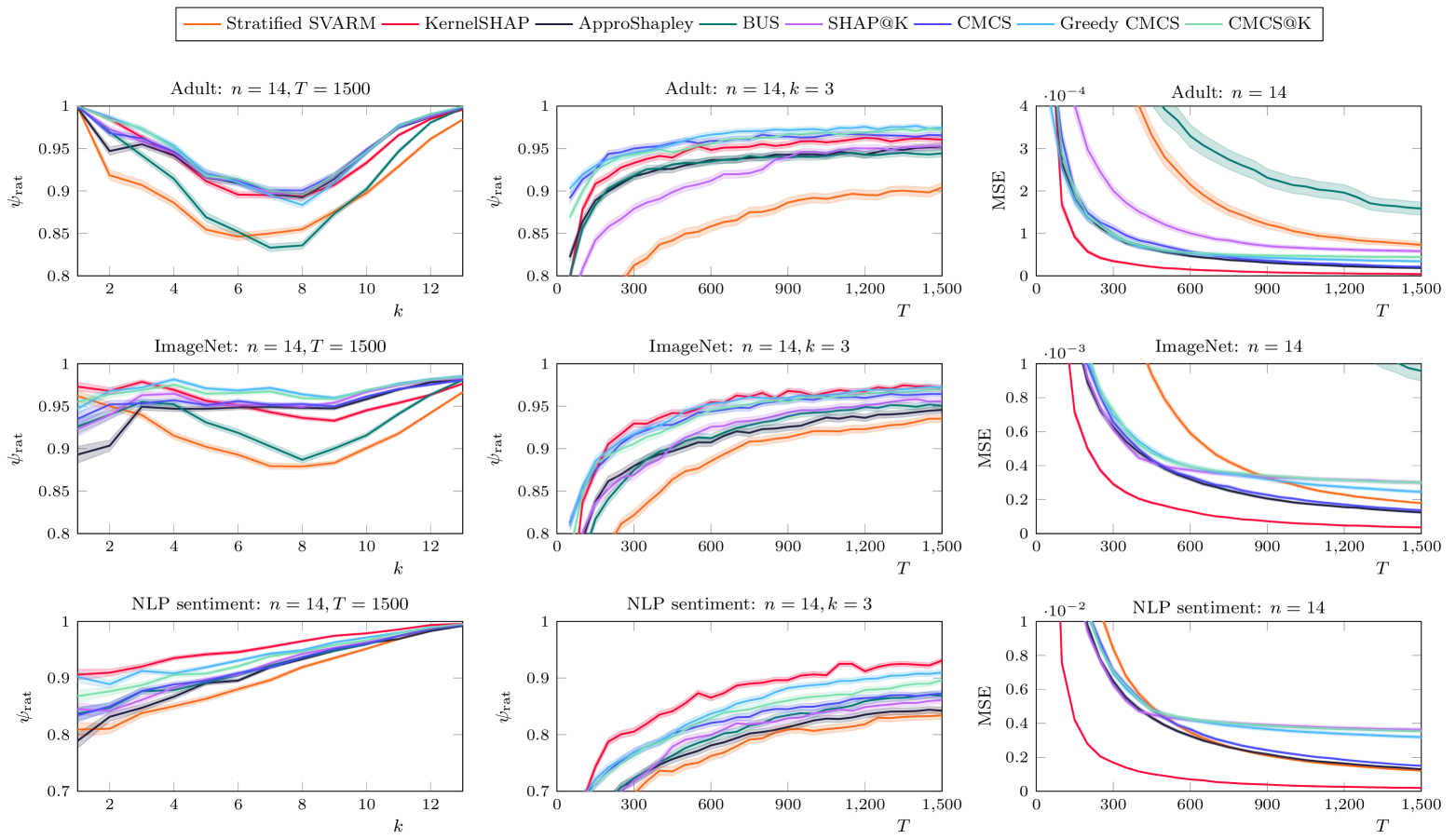
Figure 8: Comparison of achieved ratio precision and MSE with baselines for local explanations: precision for fixed budget with varying $k$ (left), precision for fixed $k$ with increasing budget (middle), and MSE depending on budget (right).

References

- Bubeck et al. (2013) Bubeck, S., Wang, T., and Viswanathan, N. Multiple identifications in multi-armed bandits. In Proceedings of the 30th International Conference on Machine Learning (ICML), pp. 258–265, 2013.
- Burgess & Chapman (2021) Burgess, M. A. and Chapman, A. C. Approximating the shapley value using stratified empirical bernstein sampling. In Proceedings of the Thirtieth International Joint Conference on Artificial Intelligence, IJCAI, pp. 73–81, 2021.
- Castro et al. (2009) Castro, J., Gómez, D., and Tejada, J. Polynomial calculation of the shapley value based on sampling. Computers & Operations Research, 36(5):1726–1730, 2009.
- Castro et al. (2017) Castro, J., Gómez, D., Molina, E., and Tejada, J. Improving polynomial estimation of the shapley value by stratified random sampling with optimum allocation. Computers & Operations Research, 82:180–188, 2017.
- Chen et al. (2023) Chen, H., Covert, I. C., Lundberg, S. M., and Lee, S. Algorithms to estimate shapley value feature attributions. Nature Machine Intelligence, 5(6):590–601, 2023.
- Cohen et al. (2007) Cohen, S. B., Dror, G., and Ruppin, E. Feature selection via coalitional game theory. Neural Comput., 19(7):1939–1961, 2007.
- Covert & Lee (2021) Covert, I. and Lee, S.-I. Improving kernelshap: Practical shapley value estimation using linear regression. In The 24th International Conference on Artificial Intelligence and Statistics AISTATS, volume 130 of Proceedings of Machine Learning Research, pp. 3457–3465, 2021.
- Covert et al. (2019) Covert, I., Lundberg, S., and Lee, S.-I. Shapley feature utility. In Machine Learning in Computational Biology, 2019.
- Covert et al. (2020) Covert, I., Lundberg, S. M., and Lee, S. Understanding global feature contributions with additive importance measures. In Proceedings of Advances in Neural Information Processing Systems (NeurIPS), 2020.
- Deng & Papadimitriou (1994) Deng, X. and Papadimitriou, C. H. On the complexity of cooperative solution concepts. Math. Oper. Res., 19(2):257–266, 1994.
- Doumard et al. (2022) Doumard, E., Aligon, J., Escriva, E., Excoffier, J., Monsarrat, P., and Soulé-Dupuy, C. A comparative study of additive local explanation methods based on feature influences. In Proceedings of the International Workshop on Design, Optimization, Languages and Analytical Processing of Big Data (DOLAP), pp. 31–40, 2022.
- Gabillon et al. (2011) Gabillon, V., Ghavamzadeh, M., Lazaric, A., and Bubeck, S. Multi-bandit best arm identification. In Proceedings in Advances in Neural Information Processing Systems (NeurIPS), pp. 2222–2230, 2011.
- Ghorbani & Zou (2019) Ghorbani, A. and Zou, J. Y. Data shapley: Equitable valuation of data for machine learning. In Proceedings of the 36th International Conference on Machine Learning ICML, volume 97, pp. 2242–2251, 2019.
- Ghorbani & Zou (2020) Ghorbani, A. and Zou, J. Y. Neuron shapley: Discovering the responsible neurons. In Proceedings of Advances in Neural Information Processing Systems (NeurIPS), 2020.
- Goldwasser & Hooker (2024) Goldwasser, J. and Hooker, G. Stabilizing estimates of shapley values with control variates. In Proceedings of the Second World Conference on eXplainable Artificial Intelligence (xAI), pp. 416–439, 2024.
- Illés & Kerényi (2019) Illés, F. and Kerényi, P. Estimation of the shapley value by ergodic sampling. CoRR, abs/1906.05224, 2019.
- Kariyappa et al. (2024) Kariyappa, S., Tsepenekas, L., Lécué, F., and Magazzeni, D. Shap@k: Efficient and probably approximately correct (PAC) identification of top-k features. In Proceedings of AAAI Conference on Artificial Intelligence (AAAI), pp. 13068–13075, 2024.
- Kolpaczki et al. (2021) Kolpaczki, P., Bengs, V., and Hüllermeier, E. Identifying top-k players in cooperative games via shapley bandits. In Proceedings of the LWDA 2021 Workshops: FGWM, KDML, FGWI-BIA, and FGIR, pp. 133–144, 2021.
- Kolpaczki et al. (2024a) Kolpaczki, P., Bengs, V., Muschalik, M., and Hüllermeier, E. Approximating the shapley value without marginal contributions. In Proceedings of AAAI Conference on Artificial Intelligence (AAAI), pp. 13246–13255, 2024a.
- Kolpaczki et al. (2024b) Kolpaczki, P., Haselbeck, G., and Hüllermeier, E. How much can stratification improve the approximation of shapley values? In Proceedings of the Second World Conference on eXplainable Artificial Intelligence (xAI), pp. 489–512, 2024b.
- Lattimore & Szepesvári (2020) Lattimore, T. and Szepesvári, C. Bandit Algorithms. Cambridge University Press, 2020. ISBN 9781108486828.
- Lundberg & Lee (2017) Lundberg, S. M. and Lee, S.-I. A unified approach to interpreting model predictions. In Proceedings of Advances in Neural Information Processing Systems (NeurIPS), pp. 4768–4777, 2017.
- Maleki et al. (2013) Maleki, S., Tran-Thanh, L., Hines, G., Rahwan, T., and Rogers, A. Bounding the estimation error of sampling-based shapley value approximation with/without stratifying. CoRR, abs/1306.4265, 2013.
- Mitchell et al. (2022) Mitchell, R., Cooper, J., Frank, E., and Holmes, G. Sampling permutations for shapley value estimation. Journal of Machine Learning Research, 23(43):1–46, 2022.
- Molnar (2022) Molnar, C. Interpretable Machine Learning. 2 edition, 2022. URL https://christophm.github.io/interpretable-ml-book.
- Narayanam & Narahari (2008) Narayanam, R. and Narahari, Y. Determining the top-k nodes in social networks using the shapley value. In Proceedings of International Joint Conference on Autonomous Agents and Multiagent Systems (AAMAS), pp. 1509–1512, 2008.
- O’Brien et al. (2015) O’Brien, G., Gamal, A. E., and Rajagopal, R. Shapley value estimation for compensation of participants in demand response programs. IEEE Transactions on Smart Grid, 6(6):2837–2844, 2015.
- Okhrati & Lipani (2020) Okhrati, R. and Lipani, A. A multilinear sampling algorithm to estimate shapley values. In 25th International Conference on Pattern Recognition ICPR, pp. 7992–7999, 2020.
- Pelegrina et al. (2025) Pelegrina, G. D., Kolpaczki, P., and Hüllermeier, E. Shapley value approximation based on k-additive games. CoRR, abs/2502.04763, 2025.
- Rozemberczki & Sarkar (2021) Rozemberczki, B. and Sarkar, R. The shapley value of classifiers in ensemble games. In The 30th ACM International Conference on Information and Knowledge Management CIKM, pp. 1558–1567, 2021.
- Rozemberczki et al. (2022) Rozemberczki, B., Watson, L., Bayer, P., Yang, H.-T., Kiss, O., Nilsson, S., and Sarkar, R. The shapley value in machine learning. In Proceedings of the Thirty-First International Joint Conference on Artificial Intelligence IJCAI, pp. 5572–5579, 2022.
- Shapley (1953) Shapley, L. S. A value for n-person games. In Contributions to the Theory of Games (AM-28), Volume II, pp. 307–318. Princeton University Press, 1953.
- van Campen et al. (2018) van Campen, T., Hamers, H., Husslage, B., and Lindelauf, R. A new approximation method for the shapley value applied to the wtc 9/11 terrorist attack. Social Network Analysis and Mining, 8(3):1–12, 2018.
- Vilone & Longo (2021) Vilone, G. and Longo, L. Notions of explainability and evaluation approaches for explainable artificial intelligence. Information Fusion, 76:89–106, 2021.
- Wang et al. (2024) Wang, H., Liang, Q., Hancock, J. T., and Khoshgoftaar, T. M. Feature selection strategies: a comparative analysis of shap-value and importance-based methods. Journal of Big Data, 11(1):44, 2024.