| Free Probability Theory | Tensor Free Probability Theory | Reference | ||||
|
|
LABEL:def:tensor-ncps | ||||
|
|
LABEL:def:tensor-ncps | ||||
|
|
LABEL:def:free-tensor-cumulants | ||||
|
|
LABEL:def:tensor-freeness | ||||
|
|
LABEL:thm-locui-tensorfree | ||||
|
|
LABEL:thm-TensorCLT |
On the applicative level, we apply the results obtained to study the asymptotic behavior of families of random matrices having various distributional symmetries and independence structures. The common feature of these random matrix models is that the corresponding linear operators act on -partite tensor products of vector spaces. We prove that, under various hypotheses:
-
–
Independent and unitarily invariant families are asymptotically tensor free (LABEL:cor-UITensorFree). Similar results hold for orthogonally invariant random matrices (LABEL:cor-OITensorFree).
-
–
Independent and local unitarily invariant families are asymptotically tensor free (LABEL:thm-locui-tensorfree). Similar results hold for orthogonally invariant random matrices (LABEL:thm-LocOI-tensorfree).
-
–
Partial transpositions of unitarily invariant random matrices are asymptotically tensor free (LABEL:thm-LocUITranspose). Similar results hold for independent families (LABEL:thm-indepTranspose) and orthogonally invariant random matrices (LABEL:thm-OITranspose).
-
–
Tensor embeddings of a bipartite unitarily invariant random matrix are asymptotically tensor free (LABEL:thm:embed-different-spaces).
-
–
Tensor freely independent, identically distributed elements satisfy a tensor free central limit theorem (LABEL:thm-TensorCLT). In the bipartite case, we obtain the distribution of the central limit (LABEL:thm-CLTBipartite).
Our work considers exclusively matrices acting on a tensor product vector space, whereas the recent articles [KMW24, BB24, collins2024free] deal with tensors of arbitrary rank. This focus allows us to follow closely Speicher’s combinatorial formulation of Voiculescu’s free probability theory, providing us with the tools to investigate relevant problems in random matrix theory related to multi-matrix models and their partial transpositions, as well as tensor generalizations of cornerstone results in non-commutative probability theory such as the tensor free central limit theorem.
Importantly, the notion of tensor distribution is richer than the usual notion of distribution from non-commutative probability theory, since it encapsulates a larger class of trace invariants. This means that the associated notion of freeness, tensor freeness, is different than Voiculescu’s free independence. Although tensor freeness corresponds to the usual notion of freeness in the matrix case (), we show in LABEL:ex-TensorFreeNonFree that already for , there are examples of tensor freely independent elements that are not free in the usual sense. In the case of multipartite random matrices having (global) unitary invariance, the two notions are equivalent asymptotically, see LABEL:thm-ui-tensorfree and LABEL:thm-oi-tensorfree for the orthogonal case. Let us also mention that in the case of tensor embeddings of bipartite random matrices, tensor free independence captures more general situations (LABEL:thm:embed-different-spaces) than Voiculescu’s freeness (LABEL:cor:embeddings-free).
Having established that tensor distributions and tensor free independence capture more general situations than the usual notions of non-commutative distributions and free independence, we would like to point out the newly introduced concepts allow us, in some cases, to obtain results about free (asymptotic) independence. This is the case, for example, in LABEL:thm-indepTranspose (part (2)), LABEL:thm-OITranspose, and LABEL:cor:embeddings-free. These results are either new or generalize previously known facts about the asymptotic freeness of certain classes of random matrices. Their proofs depend crucially on the newly introduced concept of tensor free independence, which provides a unified combinatorial framework capable of analyzing the asymptotic behavior of various random matrix models with tensor structures.
We present below two of the main results of this work that we also touched upon in •.
First, let us state in more detail our main result regarding the asymptotic tensor freeness of independent families of random (local) unitarily invariant families of random matrices.
Theorem 1.1 (LABEL:thm-indepTranspose, Asymptotic tensor freeness of (local) unitary invariant random matrices).
Let be independent families of random matrices, and let us identify .
-
(1)
If each is local unitary invariant, has tensor factorization property LABEL:eq-condition-TensorFact, and converges in tensor distribution, then the families of all partial transposes ( {(t_1⊗⋯⊗t_r)(X_N^(i)): t_1,…, t_r∈{id_N, ⊤} })_i∈[L] are asymptotically tensor free as , where is the transpose map.
-
(2)
If each is unitary invariant, has the factorization property LABEL:eq-condition-Fact, and converges in distribution, then all the random matrices are both asymptotically free and asymptotically tensor free as .
This result actually follows from a combination of two special cases. First, when partial transposition is not considered, we recover the tensor free independence between independent, LUI matrices (LABEL:thm-locui-tensorfree). Second, in the case and , the existence of tensor distribution limit of automatically guarantees the existence of joint limit distribution of the family , under the assumption of local unitary invariance, and further implies (tensor) freeness between them when is globally UI (LABEL:thm-LocUITranspose). In particular, this recovers and generalizes the previous findings from [MP24, PY24]. Additionally, we establish analogous results for (local) orthogonal invariant random matrices; we refer to LABEL:thm-oi-tensorfree, LABEL:thm-LocOI-tensorfree and LABEL:thm-OITranspose,
Secondly, we present our main results regarding the tensor free central limit theorem.
Theorem 1.2 (LABEL:thm-TensorCLT and LABEL:thm-CLTBipartite, Central limit theorems for tensor free elements).
Let be a family of identically tensor distributed, and tensor free elements in an -partite algebraic tensor probability space . Furthermore, suppose for all . Then we have x1+⋯+xN-Nφ(x1)N→∑_α∈(S_2)^r∖{id_2} κ_α(x_1) s_α in tensor distribution as , where are tensor free family of semicircular elements.
In the bipartite case (), the limiting random variable above has (usual) distribution (D_κ_γ_2,id_2(x_1)[μ_SC] * D_κ_γ_2,id_2(x_1)[μ_SC])⊞D_κ_γ_2,γ_2(x_1)[μ_SC], where denotes the classical convolution, denotes the (additive) free convolution, is the standard semicircular distribution, and denotes the dilation operator.
In the framework of tensor free probability, the central limit is characterized not by a single universal element but by a linear combination of semicircular elements , with coefficients determined by the tensor free cumulants of order 2 of the variables . Actually, the family can always be constructed as the limit of tensor GUE models and turns out to be -free [CC21, CGVH24] for some choice of an adjacency matrix ; see LABEL:rmk-TensorCLT for details. Moreover, our result for the bipartite case recovers and extends the previous results on tensor products of free variables [LSY24, Sko24], as discussed in LABEL:sec-CLTProdFree.
Note that our results are restricted to first-order behavior. In particular, the assumptions we require for tensor freeness in this paper are minimal in some sense. The study of higher-order limits [CMSS07, collins2024free] and strong convergence is postponed for future work.
This paper is organized as follows. Section 2 reviews preliminary concepts including permutations, partitions, free cumulants, Weingarten calculus, and distributional symmetries of random matrices. LABEL:sec-TensorNCPS introduces the algebraic framework of -partite tensor probability spaces based on tensor trace invariants and defines convergence in tensor distribution. LABEL:sec:tensor-free-cumulants defines tensor free cumulants as a generalization of free cumulants using moment-cumulant formulas involving permutation tuples. LABEL:sec:tensor-free-independence introduces the central concept of tensor free independence, characterized by vanishing mixed tensor free cumulants, and examines its fundamental properties. LABEL:sec-UItensorfree is dedicated to the study of globally invariant random matrices from a tensor free probability perspective. In LABEL:sec-LocUITensorFree we present a key result showing that independent, locally invariant random matrices that converge in tensor distribution are asymptotically tensor free and discuss further asymptotic properties of LUI random matrices. In LABEL:sec-TensorFreeNonIndep we consider models of non-independent matrices, proving asymptotic tensor freeness for partial transposes (LABEL:thm-indepTranspose) and tensor embeddings (LABEL:thm:embed-different-spaces) of certain random matrices. Finally, LABEL:sec:tensor-free-CLT develops a tensor free central limit theorem (LABEL:thm-TensorCLT), demonstrating convergence towards a combination of tensor free semicircular elements.
2. Background on random matrix theory and free probability
In this section, we provide several preliminary notions and results from combinatorics, random matrix theory, and free probability. We also introduce notation used throughout the paper.
2.1. Permutations and partitions
Throughout this paper, we denote by the symmetric group acting on a finite set and by the symmetric group of order , where . For , we use to denote the number of disjoint cycles in and to denote the length of , that is, the minimum number of transpositions whose product equals . Both and depend only on the conjugacy class of , and they satisfy the relation . The notation is used in this paper exclusively to denote the length of permutations and not for cardinality of sets; we use for the latter. For these basic statistics on , we refer the reader to [nica2006lectures, Lecture 23]. Moreover, we use the notation γ_p:=(1 2 ⋯ p)∈S_p for the full cycle permutation and we shall denote by the set of cycles of the permutation (including singletons).
The length function induces the metric on , , from the fact that it satisfies the triangle inequality for all and if and only if (where denotes the identity permutation), see [nica2006lectures, Proposition 23.9]. Let us define the following partial order relation on : if they satisfy the equality
| (1) |
i.e. the path is a geodesic. Then it is straightforward to check that is a partially ordered set. For , let us denote by the set of permutations such that .
Let the set of all partitions of the finite set . If is totally ordered, we denote by the set of non-crossing partitions of , that is partitions for which there do not exist such that and ; we refer the reader to [nica2006lectures, Lectures 9 and 10] for the combinatorics of non-crossing partitions. Furthermore, denotes the set of all pair partitions (or pairings) of , i.e. partitions all whose blocks are of size . As before, we simply denote by , , and when . We again denote by the reversed refinement order for partitions, i.e. if each block of is completely contained in one of the blocks of . Note that is a lattice: for all two partitions , there exists
-
(1)
the join which is a minimum partition satisfying and ,
-
(2)
the meet which is a maximum partition satisfying and .
The poset is also a lattice [nica2006lectures, Proposition 9.17], and both sets and share the same minimum partition and maximum partition . On the other hand, the two join operations on and on are distinct in general: if we take two non-crossing partitions in , then while . However, we always have .
The set can be completely described through the comparison with the non-crossing partitions. To this end, let be the natural projection map by identifying each cycle of as a block of , by discarding the order of its elements. Furthermore, let us denote the disjoint product of permutations by , and analogously the disjoint concatenation of partitions . For example, we can write the cycle decomposition of as when each is a full cycle on a set and .
The following facts are well-known in combinatorics. We refer to [biane1997some, nica2006lectures, mingo2017free] for the proof.
Proposition 2.1.
For the full cycle , the map induces the natural order isomorphism between and . Specifically,
-
(1)
if and only if and every cycle of can be written in the form for ,
-
(2)
For , if and only if .
Proposition 2.2.
Let and be the cycle decomposition of . Then , in the sense that if and only if we can write for some for each . In particular, induces a lattice structure on for every permutation .
Furthermore, elements in are completely determined by their associated partitions: if and , then .
As an example, for a permutation , we have
the last three relations fail, respectively, because: and do not belong to the same cycle of , the cycles and are crossing in , and the cycle is ordered differently in .
Thanks to the lattice structure on , the join and meet operations on is well-defined. We remark that the meet operation is independent of the choice of : if , then . However, join operation may depend on : if are α=(1 2)(3 4 5), β=(2 3), σ=γ_5, σ’=(1 2 5 3 4), then , but while .
In this paper, we shall often consider tuples of permutations and partitions in many kinds of computations. We shall use underlined symbols to denote such tuples of objects. For example, we usually denote permutations and partitions by Greek letters, e.g. and ; an -tuple of permutations and partitions will be denoted thus by and , etc. In other words, and . Furthermore, we naturally extend the operations on tuples of permutations or partitions in a component-wise manner: for instance,
for , , , and . Since most of our work is about generalizing Voiculescu’s free probability theory (and especially Speicher’s combinatorial approach to it) to the -tensor setting, this notation will be very useful in our work. Most of the combinatorial machinery of free probability theory (moments, cumulants, non-crossing partitions, etc) will be generalized to the -tensor setting by replacing the objects in the free case by -tuples of objects in the tensor free case.
Definition 2.3.
For positive integers , we endow the set of -tuples of permutations of elements with a partial order, as follows: for , α≤β if ∀s ∈[r], —α_s— + —α_s^-1 β_s— = —β_s—. In other words, if for all , the permutation lies on the geodesic between the identity permutation and the permutation . We also write .
With this definition, the poset is the -times direct product (see [nica2006lectures, Definition 9.27]) of the poset . Using the characterization of geodesics in from Propositions 2.1 and 2.2, we can describe the partial order on even more explicitly: if the following conditions hold for all :
-
–
every cycle of is contained inside some cycle of (as sets)
-
–
the cycles of induce non-crossing partitions on the cycles of
-
–
the cycles of have the same cyclic order as the cycles of they belong to.
Note that the poset is not a lattice for and . For example, in the two full cycles and do not admit a common larger element: and similarly for . The same two full cycles do not admit a largest common smaller element: the three transpositions , , and are all common smaller elements, and maximal with respect to . This is in contrast with the case of the poset of non-crossing partitions, which is a lattice. In a similar vein, for all permutations , the poset is a lattice, see Proposition 2.1.
Let us further collect several properties of pairings discussed in [MP13, MP19]; these properties will be particularly useful in the study of transpositions of random matrix models and, more generally, in the study of random matrix models with orthogonal invariance. First, we denote by the set of pairings on the set , where . Throughout this paper, we will fix the pairing and consider two natural embeddings
-
(1)
, (identifying each pair as a transposition),
-
(2)
, .
Following these identifications, one can consider two other embeddings
-
(1)
, ,
-
(2)
, ,
as in [MP19, collins2024free]. Here the multiplications above are well-defined in . One can greatly benefit from these identifications when we deal with the join operation between two pairings, as shown in the lemmas below.
Lemma 2.4 ([MP13, Lemma 2]).
Let be pairings and a cycle of . Let . Then is also a cycle of , these two cycles are distinct, and is a block of . In particular: 2⏟#(π∨ρ)_number of blocks ofthe partition =⏟#(πρ)_number of cycles ofthe permutation .
Lemma 2.5 ([MP19, Section 5]).
The map is a bijection from onto , the set of pairings such that for all (or equivalently, leaves invariant: ). Furthermore, is the inverse map.
Recall from the definition of disjoint product that is the set of permutations such that for each . In particular, , every element satisfies , and all such commute with each other.
Lemma 2.6.
-
(1)
For every , one can write or equivalently, πδ=(εσε)δ(εσε)^-1δ=εσδσ^-1δε, for some and . Moreover, we have .
-
(2)
For and , we have if and only if there exists such that . Moreover, the corresponding is uniquely determined.
-
(3)
For , we have if and only if there exists and such that and π=εσδσ^-1ε, ρ=ετδτ^-1ε.
Proof.
(1) According to Lemma 2.4, the cycle decomposition of is of the form , where the cycle induces another cycle . Since all the cycles commute, we can write πδ=(c_1⋯c_l)δ(c_1⋯c_l)^-1δ. Note that the permutation stabilizes a set (i.e., ) having cardinality and since and are disjoint cycles acting on the same set up to opposite signs. Therefore, we can find a permutation such that stabilizes the set , i.e., . Since commutes with , we have πδ=(εσε)δ(εσε)^-1δ=εσδσ^-1δε. Moreover, we have since and have disjoint cycle decompositions (after ignoring all singletons).
(2) Since leaves invariant, Proposition 2.2 implies that also leaves invariant. Therefore, Lemma 2.5 implies that there exists unique such that . Furthermore, again by Proposition 2.2.
(3) Let us write as in (1). Then the condition is equivalent to
since and commute. Therefore, the conclusion follows from (2). ∎
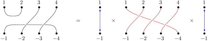
We present in Fig. 1 the decomposition of the pairing according to the result above: (1 2)(-2 3)(-3 4)(-1 -4) = ⏟(-1 1)_ε ⋅⏟(1 2 3 4)_σ ⋅δ⋅(1 2 3 4)^-1 ⋅(-1 1).
2.2. Moments and free cumulants associated to permutations
Let us recall basic notions from Free Probability Theory; the reader can consult the reference texts [voiculescu1992free, nica2006lectures, mingo2017free] for further information. A non-commutative probability space consists of a unital algebra over and a unital linear functional (called an expectation or a state). For our purposes, we always assume that is tracial, i.e. for all . Elements in are called non-commutative random variables. The distribution of a family is the data of (joint) moments , where runs over all non-commutative complex polynomials on finitely many variables, evaluated on entries from . Using linearity, the state is completely determined by moments of monomials φ(x_1 ⋯x_p); p≥1, ,x_1,…, x_p∈A. For a set , unital subalgebras of are called freely independent (or free) if every alternating product of centered elements is centered, i.e., x_i∈A_f(i), φ(x_i)=0 for and for ⟹φ(x_1⋯x_p)=0. Furthermore, subsets are called free if the unital algebras generated by each are free. The definition of freeness provides a universal rule to compute the joint distribution of (resp. ) in terms of marginal distributions of (resp. ) ([nica2006lectures, Lecture 5]).
We sometimes consider the case where has an involution , which is conjugate-linear and for . We call a -probability space if it is non-commutative probability space with an involution and for all . Then the -distribution of is defined as the distribution of and the -free independence between is defined as the freeness between . However, for full generality, non-commutative probability spaces in this paper have the minimal structure and may not necessarily have an involution unless otherwise specified.
The notion of free cumulants, introduced by Speicher [speicher1994multiplicative], provides a useful tool when we deal with free independence. For each and permutation , we first associate a multilinear functional defined by
| (2) |
For example, we have φ_(13)(624)(5)(x_1,…, x_6)=φ(x_1x_3)φ(x_6 x_2 x_4) φ(x_5), φ_γ_p(x_1,…, x_p)=φ(x_1⋯x_p). This notation mimics the one when the algebra is a matrix algebra, and the functional is the trace; see e.g. LABEL:eq-SingleTraceInv.
Then for , we define the free cumulants as multilinear functionals satisfying the so-called free moment-cumulant relation
| (3) |
From the Möbius inversion formula over each lattice , one can invert the above relation and write the formula of in terms of ’s:
| (4) |
where the Möbius function is defined by M¨ob(σ) := ∏_c ∈Cycles(σ) (-1)^—c— Cat_—c— with the Catalan numbers (recall that the length of a cycle equals the cardinality of minus ). In particular, this shows that the implicit definition of free cumulant from Eq. 3 does not depend on the permutation . Finally, we denote by and for simplicity. Let us recall the multiplicativity of and [nica2006lectures, Lecture 11]: for , , and ,
The free cumulants are the free analogs of classical cumulants , where is the set of (complex-valued) random variables with respect to a probability space having finite moments of all orders (see [nica2006lectures, Examples 1.4.(1) and Definition 11.28]). The classical moment-cumulant relations correspond to
for , where and denotes the Möbius function associated from the lattice (we refer to [nica2006lectures, Exercise 10.31-33]).
Let us simply write . One can also use the notations and for a non-crossing partitions , via the identification in Proposition 2.1. In this case, we have ~κ_π(x_1,…, x_p)=∏_B∈π~κ_Card(B)((x