Structural Stability in Piecewise Möbius Transformations

Abstract.

Structural stability of piecewise Mobius transformations (PMTs) is investigated from several angles. A result about structural stability restricted to the space of PMTs is obtained using hyperbolic features for the component functions and the pre-singularities set, allowing a holomorphic motion. Is it defined and analyzed for PMTs the analogous concept of J-stabilty for rational maps, finding some relations with the general structural stability. The notions of hyperbolic and expansive PMTs are defined, showing that they are not equivalent and none of them implies structural stability. Combining the previous results and analyzes, sufficient conditions are given for structural stability. Finally, an example of structural stability in the complexified tent maps family is shown.

Introduction

A piecewise map in a space is defined by respective transformations restricted to components belonging to a finite partition of the space. The study of dynamics of piecewise maps comes from a variety of contexts, such as the interval exchange transformations (see for instance [6, 23, 28]), the piecewise plane isometries (see [1, 2, 3, 5, 9, 12, 13, 17, 18, 19, 20, 21, 22]) and the piecewise contractions on $\mathbb{R}^{n}$ (see [8, 10]), in addition to having applications in engineering and relations with other areas of mathematics (see [11, 14, 21]).

The object of study in this research work is the dynamics of piecewise Möbius transformations (abbreviated by its acronym as PMTs) in the Riemann sphere, which is a barely inquired topic as it is inferred from the scarce mathematical literature published about it (see [11, 26]). Perhaps the most exciting link from other areas of mathematics with PMTs is that they arise as the monodromy maps of complex polynomial vector fields. These complex vector fields are a way of approaching Hilbert’s problem 16 (still open), which deals with the number and localization of limit cycles of real polynomial vector fields (see [11]). This link is not addressed in this paper, but it is expected that the results presented here will be helpful for research on that problem.

A first study about stability and structural stability for PMTs is worked on in [26]. In that paper, the associated group generated by the component functions has a central role. First, if the limit set of the group does not intersect the boundary of the domain partition and the component functions are fixed, continuous deformations of the boundary carries continuous deformations of the pre-singularities set as a compact set with the Hausdorff metric. Such continuity is a form of stability, but the structural stability of the PMTs dynamics is not guaranteed.

A second result in [26] shows that if the boundary of the partition is fixed with the associated group structurally stable and the boundary of the partition contained in a fundamental region of the group, then the corresponding PMT is structurally stable in the space of conformal automorphisms on the Riemann sphere.

In this paper, we will show sufficient conditions for the structural stability of PMTs unrelated to the structural stability of the associated group. To establish such conditions we will define and analyze for PMTs the hyperbolicity, the $\alpha$-expansivity, and the analogous concept of J-stability of rational functions in the Riemann sphere.

1. Piecewise Möbius Transformations

First of all, lets establish the basic definitions.

Definition 1.

A piecewise Möbius transformation (abbr. PMT) is a pair $(P,F)$ where

• $P=\left\{R_{k}\subset\widehat{\mathbb{C}}\right\}_{k=1}^{K}$ is a set of regions such that:

  • Each $R_{k}$ is a non-empty open and connected set.

  • Each $\partial R_{k}$ is the union of piecewise smooth simple closed curves.

  • $R_{k}\cap R_{j}=\emptyset$ if $k\neq j$.

  • $\bigcup_{k=1}^{K}\overline{R_{k}}=\widehat{\mathbb{C}}$.

• $F:\widehat{\mathbb{C}}\,\rotatebox[origin={c}]{90.0}{$\circlearrowleft$}$, where each component function $F|_{R_{k}}=f_{k}$ is the restriction of a conformal automorphism of $\widehat{\mathbb{C}}$ and $F$ is undefined in $\bigcup_{k=1}^{K}\partial R_{k}$.

• $P$ is minimal in relation to $F$, that is, if $\overline{R_{k}}\cap\overline{R_{j}}\neq\emptyset$ and it is a union of curves, then $f_{k}\neq f_{j}$.

Remark 1.

$F:\widehat{\mathbb{C}}\,\rotatebox[origin={c}]{90.0}{$\circlearrowleft$}$ is a shorthand notation for $F:\widehat{\mathbb{C}}\rightarrow\widehat{\mathbb{C}}$.

Definition 2.

The region of conformality of a PMT $(\left\{R_{k}\right\}_{k=1}^{K},\,F)$ is

$$R(F)=\bigcup_{k=1}^{K}R_{k}.$$

Definition 3.

The discontinuity set of a PMT $(\left\{R_{k}\right\}_{k=1}^{K},\,F)$ is

$$B(F)=\partial R(F)=\bigcup_{k=1}^{K}\partial R_{k}.$$

Remark 2.

Notice that the set $B(F)$ can be interpreted as the set of singularities of $F$, since $F$ is not defined in such set.

A central construction to understand the dynamics of PMTs is the pre-singularities set, as is it for meromorphic functions.

Definition 4.

The pre-discontinuity set of a PMT $F$ is

$$\mathcal{B}(F)=\overline{\bigcup_{n\geq 0}F^{-n}(B(F))}$$

Remark 3.

$\mathcal{B}(F)$ is the set of points that eventually lands in $B(F)$ under $F$, or accumulation of those points. Then, if $z\in\mathcal{B}(F)$, there exists $N\in\mathbb{N}$ such that $F^{N}(z)$ is undefined, or is an accumulation point of such pre-singularities.

Remark 4.

The set $\mathcal{B}(F)$ is alternatively called spiderweb of $F$ and denoted $Spid(F)$ (see [11]), because of its resemblance with the spider’s constructions in some cases. The analogous of this set is called exceptional set or simply discontinuity set in the theory of bidimensional piecewise isometries (see [16, 21]).

Analogously as in holomorphic dynamics, it can be defined the set with regular dynamics from the pre-singularities set.

Definition 5.

The regular set of a PMT $F$ is

$$\mathcal{R}(F)=\widehat{\mathbb{C}}-\mathcal{B}(F).$$

Another important set in the study of the dynamics of PMTs is the pre-singularities accumulation set, called the $\alpha$-limit set.

Definition 6.

The $\alpha$-limit set of a PMT $F$ is

$$\alpha(F)=\mathcal{B}(F)-\bigcup_{n\geq 0}F^{-n}(B(F)).$$

Analogously, it can be defined the $\omega$-limit set.

Definition 7.

The $\omega$-limit set of a PMT $F$ is $\omega(F)=\bigcup_{z\in\mathcal{R}(F)}\omega(z,F)$, where $\omega(z,F)$ is the $\omega$-limit set of $z$ under $F$.

Remark 5.

The $\omega$-limit set is not always forward invariant nor is always backward invariant, since can occur $\omega(F)\cap(\mathcal{B}(F)-\alpha(F))\neq\emptyset$ as we will see later.

Several results about the dynamics of PMTs as been obtained, they can be thought as an extension of the dictionary of Sullivan (see [26]). Below we state some of those results.

In what follows, let $F$ be a PMT.

Theorem 1.

(See [11] and [26].) $\mathcal{R}(F)$ is the set where the family $\left\{F^{n}\right\}_{n\in\mathbb{N}}$ is normal, and $\mathcal{B}(F)$ is the set where the family $\left\{F^{n}\right\}_{n\in\mathbb{N}}$ is not normal.

Theorem 2.

$\mathcal{B}(F)$ is backward invariant, $\mathcal{R}(F)$ is forward invariant, and $\alpha(F)$ is strictly backward invariant and forward invariant.

Proof.

We only prove the assertions about $\alpha(F)$. For the assertions about $\mathcal{B}(F)$ and $\mathcal{R}(F)$, see [11] and [26].

Let $z\in\alpha(F)$.

1. Suppose that $F^{-1}(z)\neq\emptyset$ and $F^{-1}(z)\nsubseteq\alpha(F)$. $F^{-1}(z)\cap B(F)=\emptyset$ for all $z$, since $F$ is undefined in $B(F)$. If $F^{-1}(z)\subset\mathcal{B}(F)-\alpha(F)$, then $z\in\mathcal{B}(F)-\alpha(F)$, a contradiction. If $F^{-1}(z)\cap\mathcal{R}(F)\neq\emptyset$, then $\left\{F^{n}\right\}_{n\geq 0}$ is normal in some $z_{0}\in F^{-1}(z)$ and also in $z$, a contradiction. Then $F^{-1}(\alpha(F))\subset\alpha(F).$

2. Suppose that $F(z)\notin\alpha(F)$. If $F(z)\in\mathcal{B}(F)-\alpha(F)$, then $z\in\mathcal{B}(F)-\alpha(F)$, a contradiction. If $F(z)\in\mathcal{R}(F)$, then $\left\{F^{n}\right\}_{n\geq 0}$ is not normal in $F(z)$ because neither is it in $z$, a contradiction. Then $F(\alpha(F))\subset\alpha(F).$

3. Can occur that $F^{-1}(z)=\emptyset$ and then $F(\alpha(F))\subsetneq\alpha(F)$. But always $\alpha(F)\subset F^{-1}(\alpha(F))$ by definition, then using incise (1) $F^{-1}(\alpha(F))=\alpha(F).$

∎

Theorem 3.

$\overset{\circ}{\alpha(F)}=\emptyset$, where $\overset{\circ}{\alpha(F)}$ denotes the interior of $\alpha(F)$.

Proof.

Suppose $\overset{\circ}{\alpha(F)}\neq\emptyset$. Then there exists an open set $U$ such that $U\subset\overset{\circ}{\alpha(F)}$. Let $z\in U$, then there exists $N\geq 0$ such that $F^{-N}(B)\cap U\neq\emptyset$. Therefore, $B\cap F^{N}(U)\neq\emptyset$, a contradiction since $\alpha(F)$ is forward invariant and $\alpha(F)\cap B=\emptyset$ by definition. ∎

Since periodic points of PMTs are fixed points of Möbius transformations, they can be classified in attracting (grouped in the set $\mathrm{Per_{attr}}(F)$), repelling ($\mathrm{Per_{rep}}(F)$), elliptic ($\mathrm{Per_{ell}}(F)$) and parabolic ($\mathrm{Per_{par}}(F)$). But also there are periodic points $z$ of period $n$ of a PMT $F$ for which there exists a neighborhood $U$ of $z$ such that $f^{n}|_{U}$ is the identity in $U$ (grouped in $\mathrm{Per_{id}}(F)$, and called periodic points of identity). Of course, the set of neutral or indifferent periodic points is $\mathrm{Per_{neu}}(F)=\mathrm{Per_{ell}}(F)\cup\mathrm{Per_{par}}(F)\cup\mathrm{Per_{id}}(F)$.

Theorem 4.

$$\mathrm{Per_{rep}}(F)\cup\mathrm{Per_{par}}(F)\subset\alpha(F)\subset\mathcal{B}(F),$$

$$\mathrm{Per_{attr}}(F)\cup\mathrm{Per_{par}}(F)\cup\mathrm{Per_{ell}}(F)\cup\mathrm{Per_{id}}(F)\subset\omega(F),$$

and

$$\mathrm{Per_{attr}}(F)\cup\mathrm{Per_{ell}}(F)\cup\mathrm{Per_{id}}(F)\subset\mathcal{R}(F).$$

Proof.

The family $\left\{F^{n}\right\}_{n\geq 0}$ is not normal in repelling and parabolic periodic points, then $\mathrm{Per_{rep}}(F)\cup\mathrm{Per_{par}}(F)\subset\mathcal{B}(F)$. But $\left\{F^{n}\right\}_{n\geq 0}$ is not completely defined in $\mathcal{B}(F)-\alpha(F)$, then $\mathrm{Per_{rep}}(F)\cup\mathrm{Per_{par}}(F)\subset\alpha(F)$.

In the other hand, the family $\left\{F^{n}\right\}_{n\geq 0}$ is normal in attracting, elliptic and identity periodic points, then $\mathrm{Per_{attr}}(F)\cup\mathrm{Per_{ell}}(F)\cup\mathrm{Per_{id}}(F)\subset\mathcal{R}(F)$.

Since the periodic points are in their own $\omega$-limit set, $\mathrm{Per_{attr}}(F)\cup\mathrm{Per_{ell}}(F)\cup\mathrm{Per_{id}}(F)\subset\omega(F)$.

Finally, for parabolic periodic points $z$ exists $w\in\mathcal{R}(F)$ such that $z\in\omega(w,F)$, then $\mathrm{Per_{par}}(F)\subset\omega(F)$. ∎

Since PMTs has a set of singularities, there are regular components that can also exhibit an analogous behavior to Baker domains of meromorphic functions.

Definition 8.

A point $z_{0}$ is a ghost-periodic of period $n$ of $F$ if $z_{0}\in F^{-N}(B)$ for some $N\geq 0$ and exists a periodic regular component $U$ of period $n$ such that $z_{0}\in\partial U$ and for all $z\in U$

$$\left(F^{n}\right){}^{k}(z)\underset{k\rightarrow\infty}{\rightarrow}z_{0}$$

The set of ghost-periodic points of $F$ is $\mathrm{Per_{ghost}}(F)$.

Remark 6.

By definition, $\mathrm{Per_{ghost}}(F)\subset\omega(F)\cap(\mathcal{B}(F)-\alpha(F))$.

We have a complete classification of the periodic regular components of PMTs.

Theorem 5.

Let $U$ be a periodic regular component of period $n$ of the PMT $F$. Then, only one of the following happens:

• Immediate basin of attraction, that is, exists an attracting periodic point $z_{0}\in U$ such that for all $z\in U$ $\lim_{k\rightarrow\infty}(f^{n})^{k}(z)=z_{0}$.

• Immediate parabolic basin, that is, exists a parabolic periodic point $z_{0}\in\alpha(F)$ such that for all $z\in U$ $\lim_{k\rightarrow\infty}(f^{n})^{k}(z)=z_{0}$.

• Immediate ghost-parabolic basin, that is, exists a ghost-periodic point $z_{0}\in\partial U$ such that for all $z\in U$ $\lim_{k\rightarrow\infty}(f^{n})^{k}(z)=z_{0}$.

• Rotation domain, that is, $F^{n}$ is an elliptic Möbius transformation in $U$.

• Neutral domain, that is, $F^{n}$ is the identity in $U$.

Remark 7.

In [26] the concepts of parabolic basin and ghost-parabolic basin was not differentiated, but now we consider that it is important to distinguish them due to their different dynamic behaviors.

To finalize this Section, it is worth mentioning that examples of PMT can be built with wandering domains, with regular components of any connectivity, with any number of regular components, with pre-discontinuity set being the entire sphere, or with pre-discontinuity set with positive area, as discussed in [26].

2. Hyperbolicity and Expansivity

It is well known that hyperbolic and structurally stable maps are closely related, or most likely equivalent in the case of rational maps. In this Section, we define and investigate the notions of hyperbolic PMTs, in order to find relations with structural stability.

Hyperbolic rational maps on $\widehat{\mathbb{C}}$ have only attracting and repelling periodic points, and every periodic Fatou component is an immediate attracting basin. The equivalent notion for PMTs can be defined using this feature.

Definition 9.

A PMT $F$ is hyperbolic if $\mathrm{Per_{attr}}(F)\neq\emptyset$, $\mathrm{Per_{neu}}(F)=\emptyset$, $\mathrm{Per_{ghost}}(F)=\emptyset$ and there are no wandering regular components.

Remark 8.

Note that the definition of hyperbolic PMT implies that every periodic regular component is an immediate attracting basin.

Remark 9.

Prohibiting the existence of wandering components in the definition of a hyperbolic PMT is necessary since those can cause non-hyperbolic dynamic behaviors. It is known of the existence of affine interval exchange transformations (abbr. AIET) with wandering components (see [6, 23]), where the component transformations are all contracting or expanding. Let us construct a PMT $F$ as extension of such AIET on $[0,1]$ to $\mathbb{C}$: take a open disc $R_{k}$ with diameter the corresponding interval of the partition of the AIET and an expanding transformation $f$ on the exterior of the discs such that $f^{-1}(R_{k})\subset R_{1}$ for each $k$ and where $R_{1}$ is the element of the partition such that $0\in\overline{R_{1}}.$ This PMT fulfills that $\mathrm{Per_{attr}}(F)\neq\emptyset$ (at least $\infty\in\mathrm{Per_{attr}}(F)$), $\mathrm{Per_{neu}}(F)=\emptyset,$ and $\mathrm{Per_{ghost}}(F)=\emptyset,$ but the wandering components accumulates in $\alpha(F)$. Therefore, there are $z\in\mathcal{R}(F)$ such that their orbits does not converge to a periodic attracting point.

Unlike hyperbolic rational maps, hyperbolic PMTs may not have repelling periodic points.

Example 1.

Let

$$F(z)=\begin{cases}\lambda z&\mathrm{if}\,z\in\mathbb{D}\\ \frac{1}{\lambda}z&\mathrm{if}\,z\in\widehat{\mathbb{C}}-\overline{\mathbb{D}}\end{cases}$$

where $\mathbb{D}=\left\{z\in\mathbb{C}:\,|z|<1\right\}$ and $\lambda\in\mathbb{D}-\left\{0\right\}$.

Then $0$ and $\infty$ are attracting fixed points with $\mathbb{D}$ and $\widehat{\mathbb{C}}-\overline{\mathbb{D}}$ as attracting basins, respectively. Since $\mathcal{B}(F)=B(F)=\partial\mathbb{D}$, there are no repelling or neutral periodic points. That is, $F$ is a hyperbolic PMT without repelling periodic points.

 

The hyperbolic behavior in PMTs is caused by the loxodromic component functions. But not all component functions have to be loxodromic for the PMTs to be hyperbolic, as shown in the following example.

Example 2.

Let

$$F(z)=\begin{cases}z+2&\mathrm{if}\,z\in\mathbb{D}\\ 2z&\mathrm{if}\,z\in\widehat{\mathbb{C}}-\overline{\mathbb{D}}.\end{cases}$$

Then $\mathcal{R}(F)=\mathbb{D}\cup(\widehat{\mathbb{C}}-\overline{\mathbb{D}})$. The only periodic component is $\widehat{\mathbb{C}}-\overline{\mathbb{D}}$, the immediate attracting basin of $\infty$ the unique attracting fixed point of $F$. The regular component $\mathbb{D}$ is preperiodic. The transformation $z\mapsto z+2$ is not loxodromic, but $F$ is clearly hyperbolic.

 

In the other hand, a PMTs with all their component functions loxodromic, is not necessarily hyperbolic.

Example 3.

Let

$$F(z)=\begin{cases}\frac{1}{2}z&\mathrm{if}\,z\in R_{1}\\ 2z&\mathrm{if}\,z\in R_{2}\end{cases}$$

where $R_{1}=\left\{z\in\mathbb{C}:\,|z-1|<1\right\}$ and $R_{2}=\widehat{\mathbb{C}}-\overline{R_{1}}$.

We have that $\mathcal{R}(F)=R_{1}\cup R_{2}$. Note that both component functions are loxodromic, but $0$ is a ghost-periodic point. Therefore $F$ is not hyperbolic.

 

For hyperbolic rational maps on $\widehat{\mathbb{C}}$, the dynamical behavior can be linked with some conditions over the post-critical set. PMTs has no critical points, however, the dynamical behavior can be related with the $\omega$-limit set.

Theorem 6.

Let $F$ a PMT. Then the following conditions are equivalent:

1. $F$ is hyperbolic.

2. $\omega(F)=\mathrm{Per_{attr}}(F)\neq\emptyset$.

Proof.

1. Let $F$ be hyperbolic. By definition of $\omega-$limit we have $\omega(F)=\mathrm{Per_{attr}}(F)\cup\mathrm{Per_{ell}}(F)\cup\mathrm{Per_{id}}(F)\cup\mathrm{Per_{par}}(F)\cup\mathrm{Per_{ghost}}(F)$. Then $\omega(F)=\mathrm{Per_{attr}}(F)\neq\emptyset$.

2. Suppose that $\omega(F)=\mathrm{Per_{attr}}(F)\neq\emptyset$. By definition of ghost-periodic point and $\omega$-limit set, $\mathrm{Per_{par}}(F)=\mathrm{Per_{ell}}(F)=\mathrm{Per_{id}}(F)=\mathrm{Per_{ghost}}(F)=\emptyset$. That is, $F$ is hyperbolic.

∎

Remark 10.

Note that if $F$ is a hyperbolic PMT, by the incise (2) of Theorem 6, we have $\omega(F)\cap\mathcal{B}(F)=\emptyset$ because there are no parabolic periodic points, no ghost-periodic points, and no wandering components.

Contrary to the conjectured equivalence between being hyperbolic and structurally stable in rational maps on the Riemann sphere, there are hyperbolic PMTs which are not structurally stable.

Example 4.

Let

$$F_{\lambda}(z)=\begin{cases}f_{1}(z)&\mathrm{if}\,z\in R_{1}\\ f_{2}(z)&\mathrm{if}\,z\in R_{2}\end{cases}$$

where $f_{1}(z)=\lambda z+\lambda$, $f_{2}(z)=\frac{6i\lambda z-1}{z+6i\lambda}$, $R_{1}=\left\{z:\,|1-z|<1\right\}$ and $R_{2}=\widehat{\mathbb{C}}-\overline{R_{1}}$. $f_{1}$ and $f_{2}$ are both loxodromic when $0<|\lambda|<1$.

Let $\lambda_{0}=\frac{1}{2}$. Then, there exists a neighborhood $\mathcal{N}_{\lambda_{0}}\subset\mathbb{C}$ such that $f_{1}$ and $f_{2}$ are loxodromic. The fixed points of $f_{1}$ are $z_{\lambda}=\frac{\lambda}{1-\lambda}$ (attracting) and $\infty$ (repelling), and the fixed points of $f_{2}$ are always $i$ (attracting) and $-i$ (repelling). Then the neighborhood $\mathcal{N}_{\lambda_{0}}$ can be adjusted in such a way that $z_{\lambda}\in R_{1}$ for all $\lambda\in\mathcal{N}_{\lambda_{0}}$. Therefore, $R_{1}$ must contain an immediate basin of attraction for the fixed point $z_{\lambda}$. Even more, for all $\lambda\in\mathcal{N}_{\lambda_{0}}$ we have $i,-i\in R_{2}$, causing that $R_{2}$ contains an immediate basin of attraction for the fixed point $i$ and that $-i\in\alpha(F)$.

For each $\lambda\in\mathcal{N}_{\lambda_{0}}$, let $A_{\lambda}$ be the immediate basin of attraction of $z_{\lambda}\in R_{1}$, $U_{\lambda}=\bigcup_{n\geq 0}F^{-n}(A_{\lambda})$ and $V_{\lambda}=\mathcal{R}(F)-U_{\lambda}$. Then, $F^{n}(z)\underset{n\rightarrow\infty}{\rightarrow}z_{\lambda}$ for all $z\in U_{\lambda}$ and $F^{n}(z)\underset{n\rightarrow\infty}{\rightarrow}i$ for all $z\in V_{\lambda}$. Therefore, $F_{\lambda}$ has only three periodic points, all of them fixed: $z_{\lambda}$, $i$ and $-i$. Furthermore, these fixed points are attracting or repelling, so $F_{\lambda}$ is hyperbolic.

On the other hand, varying $\lambda$ inside $\mathcal{N}_{\lambda_{0}}$, it can be found maps such that the immediate basin of attraction of $z_{\lambda}$ is exactly $R_{1}$, and maps such that $R_{1}$ contains several regular components. Obviously, these maps can not be conjugated. Then, there exists parameters $\lambda^{\prime}\in\mathcal{N}_{\lambda_{0}}$ where the mentioned bifurcation occurs and therefore, $F_{\lambda}$ is not structurally stable in neighborhoods $\mathcal{N}_{\lambda^{\prime}}\subset\mathcal{N}_{\lambda_{0}}$.

To understand this example, in the Figure 1 the approximations of the pre-discontinuity sets of $F_{\lambda}$ are drawn in black, and in the center of the red spots are the attracting fixed points $z_{\lambda}\in R_{1}$ and $i$, and the repelling fixed point $-i\in\alpha(F)$.

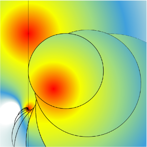
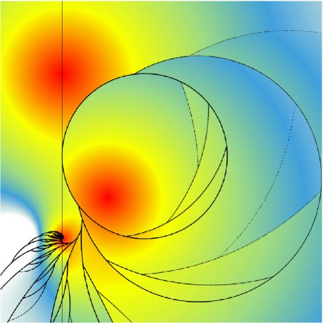
Figure 1. Pre-discontinuity an regular sets of $F_{\lambda}$ described in the Example 4.
Left: With $\lambda=\frac{1}{2}-0.223i$. $R_{1}$ is the immediate basin of attraction of $z_{\lambda}$. Right: With $\lambda=\frac{1}{2}-(0.223+\varepsilon)i$, $0<\varepsilon\ll 1$. $R_{1}$ contains several regular components.

 

For PMTs there is an analogous definition to expanding rational maps, but using points in the pre-discontinuity set where iterations of the map are always defined and also differentiable.

Definition 10.

A PMT $F$ is $\alpha$-expanding if exists $N\geq 1$ such that $|(F^{N})^{\prime}(z)|_{s}>1$ (where $|\cdot|_{s}$ is the normalized spherical norm) for all $z\in\alpha(F)$.

In contraposition to rational maps on the Riemann sphere, the characteristics of being hyperbolic and $\alpha$-expanding are not equivalent for PMTs, as it is shown in the following examples.

Example 5.

Let

$$F(z)=\begin{cases}\lambda z&\mathrm{if}\,z\in\mathbb{D}\\ \frac{1}{\lambda}z&\mathrm{if}\,z\in\widehat{\mathbb{C}}-\overline{\mathbb{D}}\end{cases}$$

where $\lambda\in\mathbb{D}-\left\{0\right\}$.

As seen previously, $F$ is hyperbolic and is not $\alpha$-expanding since $\alpha(F)=\emptyset$.

 

Example 6.

There exists $\alpha$-expanding but non-hyperbolic PMT, this because there is no incompatibility between being expanding and having elliptic, of identity, and ghost-periodic points.

Let

$$F(z)=\begin{cases}e^{\frac{2}{3}\pi i}z&\mathrm{if}\,z\in R_{1}\\ \frac{10}{9}e^{\frac{2}{3}\pi i}(1-z)&\mathrm{if}\,z\in R_{2},\end{cases}$$

where $R_{1}=\left\{z:\,|z|<\frac{1}{2}\right\}$ and $R_{2}=\widehat{\mathbb{C}}-\overline{R_{1}}$.

$R_{1}$ is a rotation domain where $0$ is an elliptic fixed point, and $z_{0}=\frac{\lambda}{\lambda+1}$, with $\lambda=\frac{10}{9}e^{\frac{2}{3}\pi i}$, is a repelling fixed point.

Clearly $\alpha(F)=\left\{z_{0}\right\}$ and then $F$ is $\alpha$-expanding but no hyperbolic.

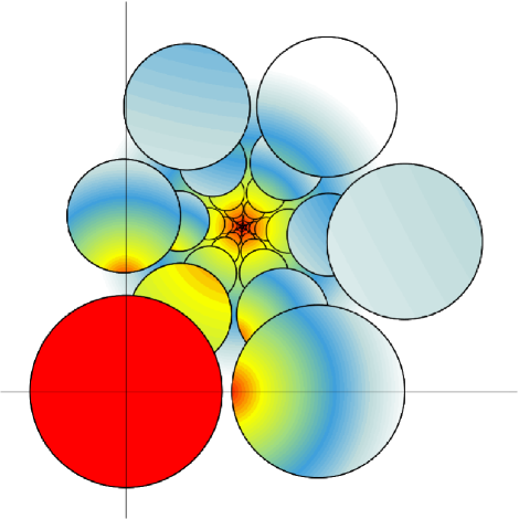
Figure 2. Pre-discontinuity set (drawn in black) and regular set (drawn with colors) of $F$ from the example 6

 

In the case of non hyperbolic and non $\alpha$-expansive PMTs, there can be estrange behaviors as the following example shows.

Example 7.

There is a non $\alpha$-expanding PMTs but with two repelling fixed points and forward invariant subsets $A\subset\alpha(F)$ such that $F|_{A}$ is conjugated with an irrational rotation. This map has no regular components.

For the PMT

$$F(z)=\begin{cases}2z&\mathrm{if}\,z\in\left\{z:\,|z|<1\right\}\\ \frac{2}{3}z&\mathrm{if}\,z\in\left\{z:\,|z|>1\right\}\end{cases}$$

it has been proven that $F|_{[\frac{2}{3},2)}$ is topologically conjugated with an irrational rotation in $S^{1}$ and $F$ behaves the same in all rays from $0$ to $\infty$ (see [26]).

Therefore, for all $z\in\left\{z\in\mathbb{C}\,:\,\frac{2}{3}\leq|z|\leq 2\right\}\cap\alpha(F)$ can not exist $N\geq 0$ such that $|F^{N}(z)|_{s}>1$ since $F|_{O(z,F)}$ is conjugated with an irrational rotation on an orbit subset of $S^{1}$.

On the other hand $\mathrm{Per}(F)=\mathrm{Fix}(F)=\left\{0,\infty\right\}$ are repelling.

 

As has been exposed, there is a non equivalence between hyperbolic and $\alpha$-expanding notions for PMTs, then, can not be studied as a single concept. The possibility of generating drastic changes in the regular set by perturbations of hyperbolic maps, makes impossible an equivalence of this notion with structural stability. Finally, the compatibility between the existence of elliptic, of identity, and ghost-periodic points and the property of being $\alpha$-expanding, implies that such maps are not necessarily structurally stable.

3. Parameter space of PMTs and conjugations

The parameter space of PMTs $F=(\left\{R_{k}\right\}_{k=1}^{K},\,\left\{f_{k}\right\}_{k=1}^{K})$ depends on the maps $F|_{R_{k}}=f_{k}\in PSL(2,\mathbb{C})$ and the elements $R_{k}$ of the partition in $\widehat{\mathbb{C}}$. For the partition, it is enough to consider the space of discontinuity sets $B=\bigcup_{k=1}^{K}\partial R_{k}$ as compact subsets of $\widehat{\mathbb{C}}$. So, we can establish the following

Definition 11.

The parameter space of PMTs over a partition of $\widehat{\mathbb{C}}$ in $K>1$ parts is

$$X_{PMT,K}=\overbrace{PSL(2,\mathbb{C})\times\dots\times PSL(2,\mathbb{C})}^{K\,\mathrm{times}}\times\mathcal{P}_{K}(\widehat{\mathbb{C}})$$

with the product topology, where $\mathcal{P}_{K}(\widehat{\mathbb{C}})$ is the space of the discontinuity sets whose associated partitions in $\widehat{\mathbb{C}}$ has $K$ parts.

Remark.

$\mathcal{P}_{K}(\widehat{\mathbb{C}})$ is a subset of the space of non-empty compact subsets of $\widehat{\mathbb{C}}$, with the Hausdorff metric. But $\mathcal{P}_{K}(\widehat{\mathbb{C}})$ can also be thought as a Teichmüller space since each $B\in\mathcal{P}_{K}(\widehat{\mathbb{C}})$ determines a set of regions $R_{k}$ which are hyperbolic Riemann surfaces, then $\mathcal{P}_{K}(\widehat{\mathbb{C}})\subset Teich(R_{1})\times Teich(R_{2})\times\dots\times Teich(R_{K})$. Moreover, $\mathcal{P}_{K}(\widehat{\mathbb{C}})$ is a complex manifold because every $R_{k}$ is a hyperbolic Riemann surface, as follows from the Bers embedding theorem (see for example [15]). In this work, the holomorphic structure of this parameter space will be very useful to us.

As usual, $F,G\in X_{PMT,K}$ are topologically conjugated if there exists a homeomorphism $h:\widehat{\mathbb{C}}\,\rotatebox[origin={c}]{90.0}{$\circlearrowleft$}$ such that $h\circ F=G\circ h$. The next result follows immediately.

Theorem 7.

If $F,G\in X_{PMT,K}$ are topologically conjugated by a homeomorphism $h:\widehat{\mathbb{C}}\,\rotatebox[origin={c}]{90.0}{$\circlearrowleft$}$, then $B(G)=h(B(F))$, $\mathcal{B}(G)=h(\mathcal{B}(F))$, $\alpha(G)=h(\alpha(F))$, and $\mathcal{R}(G)=h(\mathcal{R}(F))$.

4. Structural Stability in $PSL(2,\mathbb{C})^{K}$

In this Section, we will investigate the stability of all PMTs fixing the discontinuity set $B$ and perturbing the component functions. Then, the corresponding parameter space with this fixture is $PSL(2,\mathbb{C})^{K}\cong PSL(2,\mathbb{C})^{K}\times\left\{B\right\}\subset X_{PCM,K}$.

Now, we can establish the next

Definition 12.

A PMT $F=\left(\left\{R_{k}\right\}_{k=1}^{K},\left\{f_{k}\right\}_{k=1}^{K}\right)$ is structurally stable in $PSL(2,\mathbb{C})^{K}$ if exists a neighborhood $\mathcal{N}_{(f_{1},\dots,f_{K})}\subset PSL(2,\mathbb{C})^{K}$ such that for every element $(g_{1},\dots,g_{K})\in\mathcal{N}_{(f_{1},\dots,f_{K})}$ there exists a homeomorphism $h:\widehat{\mathbb{C}}\rightarrow\widehat{\mathbb{C}}$ such that $h\circ F=G\circ h$ in the conformality region $R(F)$, and the discontinuity set is fixed so $B(F)=B(G)$, where $G$ is the corresponding PMT $\left\{\left\{R_{k}\right\}_{k=1}^{K},\left\{g_{k}\right\}_{k=1}^{K}\right\}$.

One of the results in [26] establish the sufficiency of the structural stability in $PSL(2,\mathbb{C})^{K}$ if $\left\langle f_{1},\dots,f_{K}\right\rangle$ is a group structurally stable and the boundary set is contained in a fundamental region of such group. But indeed, such structural stability of PMTs can be obtained without any additional requirement over the group $\left\langle f_{1},\dots,f_{K}\right\rangle$ and using several strong hypotheses as stated in the following:

Theorem 8.

Let $F=\left(\left\{R_{k}\right\}_{k=1}^{K},\left\{f_{k}\right\}_{k=1}^{K}\right)$ a PMT such that

1. each component transformation $f_{k}$ is loxodromic,

2. $F$ is hyperbolic,

3. for each $k$, one of the following statements holds

   1. $f_{k}^{-1}(B(F))\cap R_{k}=f_{k}^{-1}(B(F))$,

   2. $f_{k}^{-1}(B(F))\cap R_{k}=f_{k}^{-1}(B_{j})$ for some connected component $B_{j}$ of $B(F)$, or

   3. $f_{k}^{-1}(B(F))\cap R_{k}=\emptyset$.

4. for all $n>1$ and for each connected component $C_{i}$ of $F^{-n}(B(F))$, $F^{n}(C_{i})=B_{j}$ for some connected component $B_{j}$ of $B(F)$ being $F^{n}|_{C_{i}}$ a Möbius transformation,

then $F$ is structurally stable in $PSL(2,\mathbb{C})^{K}$.

Remark 11.

Hypothesis (1) is mandatory since parabolic and elliptic Möbius transformations are not structurally stables. The hypothesis (2) are clearly necessary since the discussion from Section 2. Hypotheses (3) and (4) establishes a Schottky-like behavior for the PMT. The hypothesis (3) is exactly the hypothesis (4) for the case $n=1$, but they are stated separately for clarity.

Proof.

Small perturbations of loxodromic maps remains loxodromic, and for this very reason hyperbolic PMTs with loxodromic component functions remains hyperbolic. The action of $PSL(2,\mathbb{C})$ in $\widehat{\mathbb{C}}$ is in particular continuous, so disjoint subsets remain disjoint under the action of maps in a small neighborhood of the component functions. Thus we have that the hypotheses (1), (2), (3), and (4) allow us to take a neighborhood $\mathcal{N}_{F}=\mathcal{N}_{(f_{1},\dots,f_{K})}\subset PSL(2,\mathbb{C})^{K}$ such that for all $(g_{1},\dots,g_{K})\in\mathcal{N}_{F}$, the defined PMT $G\equiv\left\{\left\{g_{k}\right\}_{k=1}^{K},\left\{R_{k}\right\}_{k=1}^{K}\right\}$ also fulfill hypotheses (1), (2), (3), and (4).

Let $B=B(F)$. We construct $\varphi:\mathcal{N}_{F}\times E\rightarrow\widehat{\mathbb{C}}$, a holomorphic motion of $E=\left(\bigcup_{n\geq 0}F^{-n}(B)\right)\cup\mathrm{Per_{attr}}(F)$ as follows. For $\lambda=(g_{1},\dots,g_{K})\in\mathcal{N}_{F}$ with associated PMT $G$ and $z\in E$, define

$$\varphi(\lambda,z)=\begin{cases}z&\mathrm{if}\,z\in B\\ G^{-n}\circ F^{n}(z)&\mathrm{if}\,z\in F^{-n}(B),\,n>0\\ w_{z}&\mathrm{if}\,z\in\mathrm{Per_{attr}}(F)\end{cases}$$

where $G^{-n}\circ F^{n}$ is a composition $g_{k_{1}}^{-1}\circ\dots\circ g_{k_{n}}^{-1}\circ f_{k_{n}}\circ\dots\circ f_{k_{1}}$ and $w_{z}$ is the attracting fixed point of $G^{n}=g_{k_{n}}\circ\dots\circ g_{k_{1}}$ associated to the corresponding attracting fixed point $z$ of $F^{n}=f_{k_{n}}\circ\dots\circ f_{k_{1}}$.

Observe that if $z\in F^{-n}(B)$, then $F^{n}(z)\in B$ and $G^{-n}\circ F^{n}(z)\in G^{-n}(B)\subset\mathcal{B}(G)$. Using hypotheses (3) and (4) each function $\varphi_{\lambda}=\varphi(\lambda,\_)$ is an injection on $\widehat{\mathbb{C}}$ because $\varphi_{\lambda}$ is defined by one Möbius transformation in each set homeomorphic to $B$ or to $B_{j}$ (component of $B$) forming $F^{-n}(B)$, or is the identity in $B$, or is the bijection between attracting periodic points. Such bijection between attracting periodic points is possible because the hypotheses, since $F$ and $G$ have not parabolic, elliptic or of identity periodic points and regular components are preserved.

The function $\lambda\mapsto\varphi(\lambda,z)$ is a composition of the Möbius transformations $g_{1}^{-1},\dots$, $g_{K}^{-1}$, $f_{1},\dots$, $f_{K}$ with the parameters moving holomorphically, then $\varphi(\lambda,z_{0})$ is a holomorphic function on $\lambda$ for each $z_{0}\in E$. If $\lambda_{0}$ is the element associated to $F$, is clear that $\varphi(\lambda_{0},z)=z$.

Using the Bers-Royden extension theorem (see [4]), $\varphi$ has an extension to a holomorphic motion $\Phi$ of $\widehat{\mathbb{C}}$. It can be done in this way:

• First, restricting $\varphi$ to a disc $D\subset\mathcal{N}_{F}$, then transforming $D$ to $\mathbb{D}$ with an affinity, and finally restricting to $D(0,\frac{1}{3})=\left\{z:\,|z|<\frac{1}{3}\right\}$. Therefore, $\varphi|_{D(0,\frac{1}{3})\times E}$ can be extended to $\Phi:D(0,\frac{1}{3})\times\widehat{\mathbb{C}}\rightarrow\widehat{\mathbb{C}}$, as is stated in the Bers-Royden extension theorem.

• Even more, for each $\lambda\in D(0,\frac{1}{3})$, $z\mapsto\Phi(\lambda,z)$ is a quasiconformal homeomorphism $h_{\lambda}:\widehat{\mathbb{C}}\rightarrow\widehat{\mathbb{C}}$, and can be chosen in a unique manner such that the Beltrami differential $\mu(h_{\lambda})$ is harmonic in $\widehat{\mathbb{C}}-\overline{E}$. By connectivity of $\mathcal{N}_{F}$ and uniqueness of $\Phi$, the holomorphic motion $\Phi$ can be adapted and extended to $\mathcal{N}_{F}\times\widehat{\mathbb{C}}$.

By construction, $h_{\lambda}=\Phi(\lambda,\_)$ conjugates $F$ with $G$:

• If $z\in B$, then $F$ and $G$ are undefined on $z$. As $h_{\lambda}|_{B}\equiv Id|_{B}$, then $h_{\lambda}\circ F$ and $G\circ h_{\lambda}$ are undefined on $z$.

• If $z\in F^{-1}(B)$, then $F(z)\in B$. By definition of $h_{\lambda}$ by means of $\varphi$:

  • $h_{\lambda}\circ F(z)=F(z)$.

  • $G\circ h_{\lambda}(z)=G\circ G^{-1}\circ F(z)=F(z)$.

• If $z\in F^{-n}(B)$ for some $n>1$, then $F(z)\in F^{-n+1}(B)$. By definition of $h_{\lambda}$ by means of $\varphi$:

  • $h_{\lambda}\circ F(z)=G^{-n+1}\circ F^{n-1}(F(z))=G^{-n+1}\circ F^{n}(z)$.

  • $G\circ h_{\lambda}(z)=G\circ G^{-n}\circ F^{n}(z)=G^{-n+1}\circ F^{n}(z)$.

• If $z\in\mathrm{Per_{attr}}(F)$, is the attracting fixed point of some composition $f_{k_{n}}\circ\dots\circ f_{k_{1}}$. Observe that $z=F^{n}(z)\in R_{k_{1}}$, then

  1. $F(z)$ is the attracting fixed point of $f_{k_{1}}\circ f_{k_{n}}\circ\dots\circ f_{k_{2}}$. Therefore $h_{\lambda}\circ F(z)$ is the attracting fixed point of $g_{k_{1}}\circ g_{k_{n}}\circ\dots\circ g_{k_{2}}$.

  2. $h_{\lambda}(z)$ is the attracting fixed point of $g_{k_{n}}\circ\dots\circ g_{k_{1}}$ and $h_{\lambda}(z)=G^{n}(h_{\lambda}(z))\in R_{k_{1}}$. Therefore $G\circ h_{\lambda}(z)$ is the attracting fixed point of $g_{k_{1}}\circ g_{k_{n}}\circ\dots\circ g_{k_{2}}$.

• The function in $\mathcal{N}_{F}\times\widehat{\mathbb{C}}$ given by

  $$\tilde{h}_{\lambda}(z)=\begin{cases}g_{k}^{-1}\circ h_{\lambda}\circ f_{k}&\mathrm{if}\,z\in R_{k}\\ z&\mathrm{if}\,z\in B\end{cases}$$

  is also an extension of the holomorphic motion $\varphi$, with harmonic Beltrami differential since $f_{k}$ and $g_{k}^{-1}$ are holomorphic. By uniqueness of the Bers-Royden extension with such condition, we have $\tilde{h}_{\lambda}=h_{\lambda}$.

  Therefore, if $z\in\widehat{\mathbb{C}}-E$ then $z\in R_{k}$ for some $k$, and we can conclude

  $$h_{\lambda}\circ F(z)=h_{\lambda}\circ f_{k}(z)=g_{k}\circ h_{\lambda}(z)=G\circ h_{\lambda}(z).$$

∎

Remark 12.

This theorem and its proof is the foundation and inspiration of the statement and proof of the final Theorem 11, about structural stability in the general case of the parameter space $X_{PMT,K}$.

Example 8.

Let

$$F(z)=\begin{cases}f_{1}(z)&\mathrm{if}\,z\in R_{1}=\left\{z:\,|z|<\frac{2}{5}\right\}\\ f_{2}(z)&\mathrm{if}\,z\in R_{2}=\widehat{\mathbb{C}}-\overline{R_{2}}\end{cases}$$

where $f_{1}(z)=\frac{(1+i)z+i}{-iz+(1-i)}$ and $f_{2}(z)=\frac{(1+i)z-i}{iz+(1-i)}$ are loxodromic maps. $1$ is a parabolic fixed point for $F$ so do not fulfill the hyperbolicity hypothesis of the previous theorem.

On the other hand, $f_{1}$ and $f_{2}$ can be slightly perturbed so that they remain loxodromic maps and the corresponding PMT has only attracting and repelling fixed points but no parabolic fixed points. The perturbations can be made in such a way that the hypotheses of the previous theorem are fulfilled, and then all this perturbed PMTs are structurally stable in $PSL(2,\mathbb{C})^{2}$. All these perturbed PMTs have the following dynamic characteristics:

• $\mathcal{B}(F)$ is formed by the union of an infinite number of disjoint circles, union the $\alpha$-limit set.

• They have a single attracting fixed point and a single repelling fixed point, both centers of the spots colored in red.

• They have a unique immediate basin of attraction: the exterior of the discs whose boundaries form $\mathcal{B}(F)$.

• The regular components which are the interior of the disc forming $\mathcal{B}(F)$, are pre-periodic.

In the images from the Figure 3, are drawn in black the approximations of the pre-discontinuity sets of perturbations of $F$.

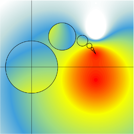
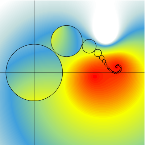
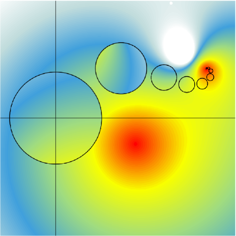
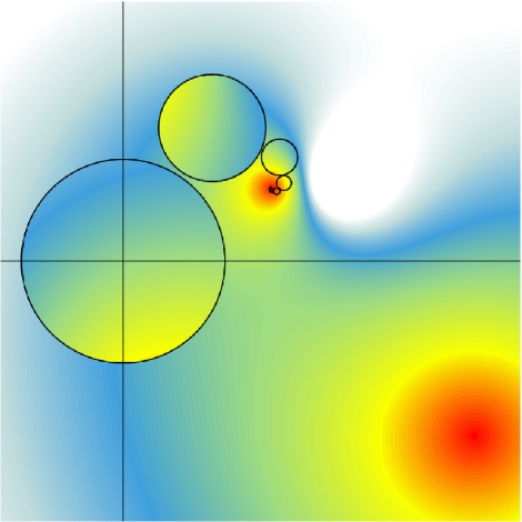
Figure 3. Pre-discontinuity and regular sets of $F$ composed by $f_{1}$ and $f_{2}$, from the Example 8.
Top left: With $f_{1}(z)=\frac{(1+i)z+1.02i}{-1.02iz+(1-i)}$ and $f_{2}(z)=\frac{(1+i)z-1.02i}{1.02iz+(1-i)}$.
Top right: With $f_{1}(z)=\frac{(1+i)z+0.99+0.01i}{-(0.99+0.01i)z+(1-i)}$ and $f_{2}(z)=\frac{(1+i)z-0.99-0.01i}{(0.99+0.01i)z+(1-i)}$.
Bottom left: With $f_{1}(z)=\frac{(1+i)z+i}{-iz+(1-i)}$ and $f_{2}(z)=\frac{(0.8+i)z-i}{iz+(1-i)}$.
Bottom right: With $f_{1}(z)=\frac{(1+i)z+i}{-iz+(1-i)}$ and $f_{2}(z)=\frac{(1.1+i)z+0.1-i}{(-0.1+i)z+(0.9-i)}$.

 

5. $\mathcal{B}$-Stability

Before the study of general structural stability of PMTs, let us define and analyze a kind of stability analogous to the J-stability of rational maps.

First, let us define holomorphic families of PMTs, where the corresponding parameter space necessarily is a complex manifold.

Definition 13.

A family of PMTs $\left\{F_{\mu,\lambda}:\widehat{\mathbb{C}}\,\rotatebox[origin={c}]{90.0}{$\circlearrowleft$}\right\}_{(\mu,\lambda)\in Y\times X}$, parameterized by $(\mu,\lambda)\in Y\times X$ where $Y$ and $X$ are complex manifolds, is a holomorphic family if

• There exists a holomorphic motion of the discontinuity set $B(F_{\mu_{0},\lambda})\in\mathcal{P}_{K}(\widehat{\mathbb{C}})$, parameterized by $(Y,\mu_{0})$ over the discontinuity sets of $F_{\mu,\lambda}$.

• The function $Y\times X\times R(F_{\mu,\lambda})\rightarrow R(F_{\mu,\lambda})$, given by $(\mu,\lambda,z)\mapsto F_{\mu,\lambda}(z)$ is holomorphic.

In an analogous way to how the holomorphic motion of Julia sets is defined, it can be defined for the pre-discontinuity sets of PMTs.

Definition 14.

Given a holomorphic family of PMTs $\left\{F_{\mu,\lambda}:\widehat{\mathbb{C}}\,\rotatebox[origin={c}]{90.0}{$\circlearrowleft$}\right\}_{(\mu,\lambda)\in Y\times X}$, the pre-discontinuity sets $\mathcal{B}(F_{\mu,\lambda})$ moves holomorphically if there is a holomorphic motion

$$\left\{\varphi_{\mu,\lambda}:\mathcal{B}(F_{\mu_{0},\lambda_{0}})\rightarrow\widehat{\mathbb{C}}\right\}_{(\mu,\lambda)\in Y\times X}$$

such that

$$\varphi_{\mu,\lambda}\left(\mathcal{B}(F_{\mu_{0},\lambda_{0}})\right)=\mathcal{B}(F_{\mu,\lambda}),$$

$$\varphi_{\mu,\lambda}\circ F_{\mu_{0},\lambda_{0}}|_{\mathcal{B}(F_{\mu_{0},\lambda_{0}})-B(F_{\mu_{0},\lambda_{0}})}=F_{\mu,\lambda}\circ\varphi_{\mu,\lambda}|_{\mathcal{B}(F_{\mu_{0},\lambda_{0}})-B(F_{\mu_{0},\lambda_{0}})},$$

and

$$\varphi_{\mu,\lambda}(B(F_{\mu_{0},\lambda_{0}}))=B(F_{\mu,\lambda}).$$

The pre-discontinuity sets $\mathcal{B}(F_{\mu,\lambda})$ moves holomorphically at $(\mu_{0},\lambda_{0})$ if they move holomorphically at some neighborhood $\mathcal{N}_{(\mu_{0},\lambda_{0})}\subset Y\times X$.

Remark 13.

Note that the holomorphic motion $\varphi_{\mu,\lambda}$ could not respect the dynamics in the entire set $\mathcal{B}(F_{\mu,\lambda})$, because of the no-definition of $F_{\mu,\lambda}$ on $B(F_{\mu,\lambda})$.

Now, it can be defined the concept of $\mathcal{B}$-stability.

Definition 15.

A PMT $F$ is $\mathcal{B}$-stable if $\mathcal{B}(F)$ moves holomorphically.

As expected, there exists PMTs that are $\mathcal{B}$-stable but not structurally stable, as it is shown below.

Example 9.

Let

$$F_{\mu,\lambda}(z)=\begin{cases}f_{1}(z)&\mathrm{if}\,z\in R_{1}\\ f_{2}(z)&\mathrm{if}\,z\in R_{2}\end{cases}$$

where $f_{1}(z)=\frac{(1+i)z+\lambda}{-\lambda z+(1-i)}$, $f_{2}(z)=\frac{(1+i)z-\lambda}{\lambda z+(1-i)}$, $R_{1}=\left\{z:\,|z-\mu|<\frac{1}{3}\right\}$ and $R_{2}=\widehat{\mathbb{C}}-\overline{R_{1}}$, with $(\mu,\lambda)\in\left\{\lambda:\,|\lambda|<\frac{1}{10}\right\}\times\left\{\mu:\,|\mu-i|<\frac{1}{10}\right\}=Y\times X.$ Clearly $F_{\mu,\lambda}$ is a holomorphic family of PMTs.

A holomorphic motion $\varphi_{\mu,\lambda}:\mathcal{B}(F_{0,i})\rightarrow\widehat{\mathbb{C}}$ can be given as

$$\varphi_{\mu,\lambda}(z)=\begin{cases}z+\mu&z\in B(F_{0,i})\\ F_{\mu,\lambda}^{-N}(F_{0,i}^{N}(z)+\mu)&z\in\mathcal{B}(F_{0,i})-\alpha(F_{0,i})\\ \frac{i-\sqrt{-1-\lambda{{}^{2}}}}{\lambda}&z\in\alpha(F_{0,i})=\left\{1\right\}\end{cases}$$

Then $\mathcal{B}(F_{0,i})$ moves holomorphically, but $F_{0,i}$ and $F_{\mu,\lambda}$ are not conjugated, for $(\mu,\lambda)$ as close to $(0,i)$ as we like.

In the Figure 4, approximations of the pre-discontinuity sets of $F_{\mu,\lambda}$ are drawn in black and fixed points are in the center of the red spots.

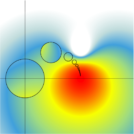
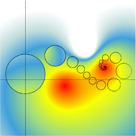
Figure 4. Holomorphic motion of $\mathcal{B}(F_{0,i})$, from the Example 9.
Left: With $\mu=0$ and $\lambda=i$, $F_{0,i}$ has a unique fixed point $z=1$, which is parabolic. Right: With $\mu\approx 0$ and $\lambda\approx i$, $F_{\mu,\lambda}$ has two fixed points: $\frac{i+\sqrt{-1-\lambda{{}^{2}}}}{\lambda}$ attracting and $\frac{i-\sqrt{-1-\lambda{{}^{2}}}}{\lambda}$ repelling.

 

Remark 14.

From the previous example, we can notice that in a holomorphic motions of PMTs parabolic points can be converted in repelling points, unlike the holomorphic motions of rational maps.

A consequence of the previous definitions and the invariance of the $\alpha$-limit set, is the next corollary.

Corollary 1.

If a PMT $F$ is $\mathcal{B}$-stable, then exists a holomorphic motion

$$\left\{\varphi_{\mu,\lambda}:\alpha(F)\rightarrow\widehat{\mathbb{C}}\right\}_{(\mu,\lambda)\in\mathcal{N}\subset Y\times X}$$

such that $\varphi_{\mu,\lambda}\left(\alpha(F)\right)=\alpha(F_{\mu,\lambda})$ and

$$\varphi_{\mu,\lambda}\circ F|_{\alpha(F)}=F_{\mu,\lambda}\circ\varphi_{\mu,\lambda}|_{\alpha(F)}.$$

Remark 15.

This corollary can be interpreted in the following way: $\mathcal{B}$-stability implies structural stability in the $\alpha$-limit set, because the corresponding holomorphic motion respects the dynamics of the $\alpha$-limit set.

As usual, the concept of $\mathcal{B}$-stability in the whole parameter space of PMTs is the $\mathcal{B}$-structural stability.

Definition 16.

A PMT $F$ is $\mathcal{B}$-structurally stable if there exists a holomorphic motion of $\mathcal{B}(F)$, parameterized by elements of a neighborhood $\mathcal{N}_{F}\subset X_{PCM,K}$.

As is expected, the analogous result for rational maps is also true for PMTs.

Theorem 9.

Let be $F$ a structurally stable PMT, then is $\mathcal{B}$-structurally stable.

Proof.

Suppose that $F$ is not $\mathcal{B}$-structurally stable. Then, given a holomorphic family $F_{\mu,\lambda}:\widehat{\mathbb{C}}\,\rotatebox[origin={c}]{90.0}{$\circlearrowleft$}$ parametrized on $\mathcal{N}_{F}\subset X_{PCM,K}$, does not exist a holomorphic motion $\varphi_{\mu,\lambda}:\mathcal{B}(F)\rightarrow\widehat{\mathbb{C}}$ such that $\varphi_{\mu,\lambda}$ respects the dynamics in $\mathcal{B}(F)-B(F)$, or $\varphi_{\mu,\lambda}(B(F))\neq B(F_{\mu,\lambda})$, for parameters close to $F$. In any case, $F$ and $F_{\mu,\lambda}$ can not be topologically conjugated, and then $F$ is not structurally stable. ∎

6. Structural Stability

For rational maps, hyperbolic (or equivalently expanding) maps are structurally stable. For PMTs, this is not the case as it has been reviewed in the Section 2.

On the other hand, we have the following

Conjecture 1.

Let $F$ be a structurally stable PMT , then it is hyperbolic and $\alpha$-expanding.

Remark.

Clearly, a structurally stable PMT can not have parabolic, elliptic, or of identity periodic points, neither ghost-periodic points, because under perturbations can be converted to attracting or repelling points. The difficulty to prove the previous conjecture are the following cases of PMTs: i) without periodic points where every regular component is wandering, ii) the case with the pre-discontinuity set dense in the sphere, or iii) the case with wandering components and the pre-discontinuity set dense in some region with positive area.

In the direction of the previous conjecture, it can be proven the next

Theorem 10.

Let $F$ a structurally stable PMT without wandering domains, then it is hyperbolic.

Proof.

Suppose that $F$ is not hyperbolic but without wandering domains. Then occurs at least one of the following:

1. $F$ has a parabolic, elliptic, or of identity periodic point $z$. Under perturbation of the component functions $f_{k}$ of $F$, $z$ can be converted to an attracting or repelling periodic point for the corresponding perturbed PMT $F_{\varepsilon}$.

2. $F$ has a ghost-periodic point $z$. Under perturbation of the discontinuity set $B$, $z$ can be converted to a periodic point of $F$, for the corresponding perturbed PMT $F_{\varepsilon}$.

3. $\mathcal{B}(F)$ contains a region $U$ of positive area and $\mathrm{Per}(F)=\emptyset$.

   1. If there exists a point $z\in\partial R_{i}\cap\partial R_{j}\cap U\subset B\cap U$, then for every neighborhood $\mathcal{N}_{z}\subset U$ exists $w\in F^{-M}(B)\cap\mathcal{N}_{z}$ for some $M>0$, because of the density of $\left(\bigcup_{N\geq 0}F^{-N}(B)\right)\cap U$ in $U$. Additionally, it can be supposed $w\in F^{-M}(B)\cap\mathcal{N}_{z}\subset R_{j}$. Then a perturbation of $B$ around $F^{M}(w)$ (and possibly also a perturbation of the component functions $f_{i}$ and $f_{j}$), can cause that $F_{\varepsilon}^{-M}(B_{\varepsilon})\cap\mathcal{N}_{z}\cap R_{i}\neq\emptyset$, where $F_{\varepsilon}$ is the corresponding perturbed PMT with $B(F_{\varepsilon})=B_{\varepsilon}$.

   2. If there exists a point $z\in F^{-N}(B)\cap U$ with $N>0$ and $z\in R_{k}$ for some $k$, then for every neighborhood $\mathcal{N}_{z}\subset U\cap R_{k}$ exists $w\in F^{-M}(B)\cap\mathcal{N}_{z}$, for some $M>0$. Let $L=\min\left\{N,M\right\}$, $z_{0}=F^{L}(z)$ and $w_{0}=F^{L}(w)$. Then, $z_{0}\in B$ or $w_{0}\in B$ and are close to each other. Hence, we have sub-case (a).

In each of the three cases, $F$ can not be topologically conjugated with its corresponding perturbed $F_{\varepsilon}$.

The “without wandering domains” hypothesis guarantees that the only case of $F$ such that $\mathrm{Per}(F)=\emptyset$ is the case (3) of the previous list. ∎

Finally, to guaranteed structural stability of a PMT, several conditions are needed.

Theorem 11.

Let $F$ be a PMT. If

1. each component function $f_{k}$ is loxodromic,

2. $F$ is hyperbolic and $\alpha$-expanding, and

3. $F$ is $\mathcal{B}$-structurally stable,

then $F$ is structurally stable.

Proof.

By hypothesis (3), exists a holomorphic family $F_{\mu,\lambda}:\widehat{\mathbb{C}}\,\rotatebox[origin={c}]{90.0}{$\circlearrowleft$}$ parametrized on $\mathcal{N}_{F}\subset X_{PCM,K}$, and a holomorphic motion $\varphi_{\mu,\lambda}:\mathcal{B}(F)\rightarrow\widehat{\mathbb{C}}$ such that $\varphi_{\mu,\lambda}$ respects the dynamics in $\mathcal{B}(F)-B(F)$ and $\varphi_{\mu,\lambda}(B(F))=B(F_{\mu,\lambda})$.

Because of hypotheses (1) and (2), a possibly smaller neighborhood $\mathcal{N}_{F}$ can be taken in such a way that each $G\in\mathcal{N}_{F}$ also meets hypotheses (1) and (2), that is, $\alpha(G)$ contains all repelling but no parabolic periodic points and $\mathcal{R}(G)$ contains all attracting but no elliptic neither of identity periodic points. Note that such PMTs $G$ are constructed with discontinuity set $B(G)=\varphi_{\mu,\lambda}(B(F))$ and the component transformations $(g_{1},\dots,g_{K})$ determined by $(\mu,\lambda)\in\mathcal{N}_{F}$.

Using the Bers-Royden extension, $\varphi$ has an extension to a holomorphic motion $\Phi$ of $\widehat{\mathbb{C}}$ such that for each $(\mu,\lambda)\in\mathcal{N}_{F}$ the function $h_{\mu,\lambda}=\Phi(\mu,\lambda,\_)$ is the unique quasiconformal homeomorphism on $\widehat{\mathbb{C}}$ with harmonic Beltrami differential in $\widehat{\mathbb{C}}-\mathcal{B}(F)$. See the proof of Theorem 8 for further details about of the construction of this extension.

By construction, $h_{\mu,\lambda}$ conjugates $F$ with $G$:

• If $z\in\mathcal{B}(F)-B$, by definition of holomorphic motion of $\mathcal{B}(F)$ we have $h_{\mu,\lambda}\circ F(z)=G\circ h_{\mu,\lambda}(z)$.

• The function in $\mathcal{N}_{F}\times\widehat{\mathbb{C}}$ given by

  $$\widetilde{h}_{\lambda}(z)=\begin{cases}g_{k}^{-1}\circ h_{\lambda}\circ f_{k}&\mathrm{if}\,z\in R_{k}\\ z&\mathrm{if}\,z\in B\end{cases}$$

  is also an extension of the holomorphic motion $\varphi$, with harmonic Beltrami differential since $f_{k}$ and $g_{k}^{-1}$ are holomorphic. By uniqueness of the Bers-Royden extension with such condition, we have $\widetilde{h}_{\lambda}=h_{\lambda}$.

  Therefore, if $z\in\mathcal{R}(F)$ then $z\in R_{k}$ for some $k$, and we can conclude

  $$h_{\lambda}\circ F(z)=h_{\lambda}\circ f_{k}(z)=g_{k}\circ h_{\lambda}(z)=G\circ h_{\lambda}(z).$$

∎

Based in experimental evidence, the equivalence between structural stability and the conditions of the previous theorem seems true. Hence a stronger conjecture than conjecture 1 above is:

Conjecture 2.

$F$ is a structurally stable PMT then each component transformation $f_{k}$ is loxodromic, $F$ is hyperbolic, and $F$ is $\alpha$-expanding.

7. Example: The Tent Maps Family

To finalize the analysis of the stability of PMTs, applications of previous results to the complex version of the well-known family of tent maps in $\mathbb{R}$ will be shown.

Definition 17.

The family of complex tent maps

$$\left\{T_{B,\lambda}:\widehat{\mathbb{C}}\,\rotatebox[origin={c}]{90.0}{$\circlearrowleft$}\right\}_{B\in\mathcal{P}_{2},\,\lambda\in\mathbb{C}-\left\{0\right\}}$$

is defined by

$$T_{B,\lambda}(z)=\begin{cases}f_{1}(z)&\mathrm{if}\,z\in R_{1}\\ f_{2}(z)&\mathrm{if}\,z\in R_{2},\end{cases}$$

where $f_{1}(z)=\lambda z$, $f_{2}(z)=\lambda-\lambda z$, $B=\partial R_{1}=\partial R_{2}$ and $\frac{1}{2}\in B$.

Remark.

The condition $\frac{1}{2}\in B$ is required to have similar behavior to the real case: $f_{1}(\frac{1}{2})=f_{2}(\frac{1}{2})=\lambda\frac{1}{2}$. Nevertheless, $T_{B,\lambda}$ can not be extended to a continuous function in every neighborhood $\mathcal{N}_{\frac{1}{2}}$.

Let us list several facts about this family of maps.

• Clearly, is a holomorphic family of PMTs.

• The fixed points of $f_{1}$ are $0$ and $\infty$. The fixed points of $f_{2}$ are $z_{\lambda}=\frac{\lambda}{\lambda+1}$ and $\infty$. Then

  $$\mathrm{Fix}(T_{B,\lambda})=\left(\left(\left\{0,\infty\right\}\cap R_{1}\right)\cup\left(\left\{z_{\lambda},\infty\right\}\cap R_{2}\right)\right)\cap\left(\mathcal{R}(T_{B,\lambda})\cup\alpha(T_{B,\lambda})\right).$$

• If $|\lambda|<1$, then $f_{1}$ and $f_{2}$ are affine contractions in $\mathbb{C}$. Therefore for almost every $\lambda\in\mathbb{D}$, all points in $\mathcal{R}(F)$ tend to an attracting or a ghost periodic orbit. Also, it can be shown that if $B\subset\mathbb{C}$, $\alpha(T_{B,\lambda})=\left\{\infty\right\}$ (see [25]).

• If $|\lambda|=1$, then $f_{1}$ and $f_{2}$ are euclidean isometries. If $B\subset\mathbb{C}$, then every point in $\mathcal{R}(F)$ is periodic or pre-periodic (see [19] for this result).

• If $\lambda=1$, then $f_{1}=Id|_{R_{1}}$ and $f_{2}$ is a euclidean rotation. If $\lambda=-1$, then $f_{1}$ is a euclidean rotation and $f_{2}$ is a translation. In any case, every point in $\mathcal{R}(F)$ is periodic or pre-periodic (see [25]).

• If $|\lambda|>1$ and $B\subset\mathbb{C}$, then $\infty$ is an attracting fixed point of $T_{B,\lambda}$.

The global behavior of the orbits can be determined with parameters such that $|\lambda|\neq 1$ (see [25]).

Theorem 12.

• If $|\lambda|<1$, $T_{B,\lambda}$ is globally attracting, that is, exists $r\in(0,\infty)$ such that if $z\in\mathcal{R}(T_{B,\lambda})-\left\{\infty\right\}$, then exists $N\in\mathbb{N}$ such that |$T_{B,\lambda}^{n}(z)|\leq r$ for all $n\geq N$.

• If $|\lambda|>1$, $T_{B,\lambda}$ is globally repelling, that is, exists $r\in(0,\infty)$ such that if $|z|>r$ and $z\in\mathcal{R}(T_{B,\lambda})$, then $\underset{n\rightarrow\infty}{\lim}T_{B,\lambda}^{n}(z)=\infty$.

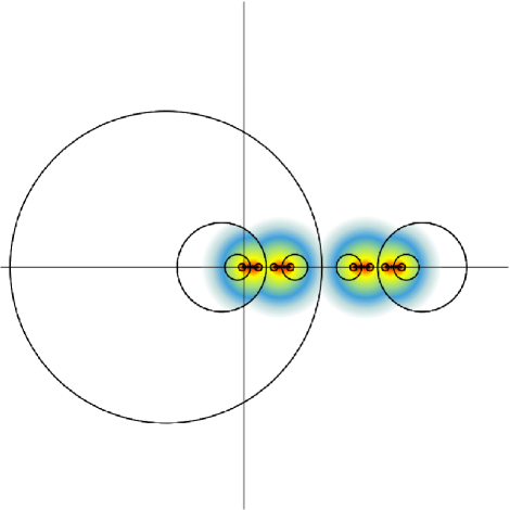
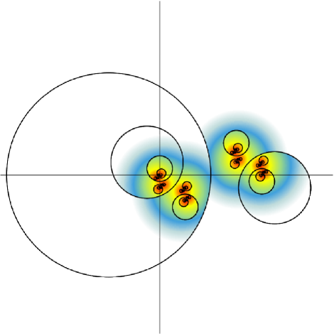
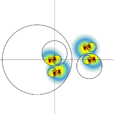
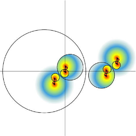
Figure 5. Pre-discontinuity and regular sets of the tent maps $T_{B,\lambda}$ from Example 10.
Top left: With $\lambda=\frac{7}{2}$. Top right: With $\lambda=2+2i$.
Bottom left: With $\lambda=\frac{11}{4}i$. Bottom right: With $\lambda=-\frac{5}{2}+2i$.

Notice that for parameters such that $|\lambda|\neq 1$, $f_{1}$ and $f_{2}$ are loxodromic and $\mathrm{Fix}(f_{1})\cap\mathrm{Fix}(f_{2})=\left\{\infty\right\}$, then the group $\Gamma=\big{<}f_{1},f_{2}\big{>}$ is not discrete. Likewise, when $\lambda=e^{2\pi\theta i}$ with $\theta$ an irrational number, $\Gamma=\big{<}f_{1},f_{2}\big{>}$ is not discrete. In any case, we have the limit set of $\Gamma$ $\Lambda(\Gamma)=\widehat{\mathbb{C}}$ and can not be applied the results about stability related to structurally stable kleinian groups (see [24, 26, 27] for this results).

However, it can be found structural stability in the family with the following conditions:

1. Parameter $|\lambda|\neq 1$.

2. Bounded discontinuity set, that is $B\subset\mathbb{C}$.

3. Finite fixed points ($0$ and $z_{\lambda}$) of $f_{1}$ and $f_{2}$ such that they are not in $B$.

4. Pre-discontinuity set formed exclusively by homeomorphic copies of $B$ and the corresponding $\alpha$-limit set. This can be achieved by taking $\lambda$ with a sufficiently big or a sufficiently small modulus.

Then, we have

• By (1), $f_{1}$ and $f_{2}$ are loxodromic.

• $T_{B,\lambda}$ has no ghost-fixed points, because $\infty,0,z_{\lambda}\notin B$ by incises (2) and (3).

• $\infty$ is an attracting or repelling fixed point of $T_{B,\lambda}$, by (1) and (2).

• $T_{B,\lambda}$ is hyperbolic and expanding. By (1) and (4):

  • Every point in $\alpha(T_{B,\lambda})$ is repelling periodic, pre-repelling periodic or with infinite orbit but being some limit point of the semi-group generated by $f_{1}^{-1}$ and $f_{2}^{-1}$.

  • Every point in $\mathcal{R}(T_{B,\lambda})$ is attracted to $\infty$ when $|\lambda|>1$, or to $0$ (if $0\in R_{1}$) or to $z_{\lambda}$ (if $z_{\lambda}\in R_{2}$) when $|\lambda|<1$.

Summarizing, $T_{B,\lambda}$ fulfilling (1), (2), (3), and (4) has loxodromic component transformations, is hyperbolic, and is expanding. Clearly, it can be constructed a holomorphic motion for each $\mathcal{B}(T_{B,\lambda})$, and then, by the Theorem 11, all these PMTs $T_{B,\lambda}$ are structurally stable.

Example 10.

The pre-discontinuity sets of $T_{B,\lambda}$ with $R_{1}=\left\{z:\,|z+\frac{1}{2}|<1\right\}$ and $R_{2}=\widehat{\mathbb{C}}-\overline{R_{1}}$ are drawn in black in the images from the Figure 5. The gradient of color indicates the proximity of repelling periodic points in $\alpha(T_{B,\lambda})$.

In this example $B$ is fixed, but it easy to see that such $B$ can be deformed according to the conditions above and the new maps are structural stable in each case.

References

- [1] P. Ashwin & X. Fu. On the geometry of orientation preserving planar piecewise isometries. J. Nonlinear Sci. 12, 207–240. (2002)
- [2] P. Ashwin & A. Goetz. Invariant Curves and Explosion of Periodic Islands in Systems of Piecewise Rotations. SIAM Journal on Applied Dynamical Systems 2005 4:2, 437-458. (2005)
- [3] P. Ashwin & A. Goetz. Cone exchange transformations and boundedness of orbits. Ergodic Theory and Dynamical Systems, 30(5), 1311-1330. (2009)
- [4] L. Bers & H.L. Royden. Holomorphic families of injections. Acta Math. 157, 259–286. (1986)
- [5] M. Boshernitzan & A. Goetz. A dichotomy for a two-parameter piecewise rotation. Ergodic Theory Dynam. Systems, 23(3):759–770. (2003)
- [6] X. Bressaud , P. Hubert, A. Maass. Persistence of wandering intervals in self-similar affine interval exchange transformations. Ergod. Th. & Dynam. Sys. vol. 30 no. 3 665-686. (2010)
- [7] X. Bressaud & G. Poggiaspalla. A Tentative Classification of Bijective Polygonal Piecewise Isometries. Exp. Math. 16(1): 77-99 (2007)
- [8] H. Bruin & J.H.B. Deane. Piecewise contractions are asymptotically periodic. Proceedings of the AMS 137, 1389-1395. (2009)
- [9] J. Buzzi. Piecewise isometries have zero topological entropy. Ergodic Theory and Dynamical Systems, 21(5), 1371-1377. (2001)
- [10] E. Catsigeras, P. Guiraud, A. Meyroneinc & E. Ugalde. On the Asymptotic Properties of Piecewise Contracting Maps. Dynamical Systems, 31:2, 107-135. (2015)
- [11] M. Cruz. Dynamics of piecewise conformal automorphisms of the Riemann sphere. Ergodic Theory and Dynamical Systems, Vol. 25, 6, 1767-1774. (2005)
- [12] J.H.B. Deane. Global attraction in the sigma-delta piecewise isometry. Dynamical Systems, vol. 17 no. 4, pp 377-388 (2002)
- [13] J.H.B Deane. Piecewise Isometries: Applications in Engineering. Meccanica 41, 241–252. (2006)
- [14] M. di Bernardo, C.J. Budd, A.R. Champneys, P. Kowalkzyk. Piecewise-smooth dynamical systems. Theory and applications. Springer. (2007)
- [15] F.P. Gardiner & N. Lakic. Quasiconformal Teichmüller Theory. Mathematical Surveys and Monographs, vol. 76, Amer. Math. Soc. (2000).
- [16] A. Goetz. Dynamics of Piecewise Isometries. PhD thesis, University of Illinois at Chicago. (1996)
- [17] A. Goetz. Dynamics of piecewise a piecewise rotation. Discrete and Continuous Dynamical Systems, 1998, 4 (4) : 593-608. (1998)
- [18] A. Goetz. First-return maps in a system of two rotations. (1999)
- [19] A. Goetz. Dynamics of piecewise isometries. Illinois J. Math. vol. 44 no. 3, 465-478. (2000)
- [20] A. Goetz. Stability of piecewise rotations and affine maps. Nonlinearity, vol. 14, no. 2. (2001)
- [21] A. Goetz. Dynamics of piecewise isometries, an emerging area of Dynamical Systems. Fractals in Graz 2001, Ed. P. Grabner and W. Woess, Birkhausser, Basel, 133-144. (2003)
- [22] A. Goetz & A. Quas. Global properties of a family of piecewise isometries. Ergodic Theory and Dynamical Systems, 29(2), 545-568. (2009)
- [23] C. Gutierrez, S. LLoyd, B. Pires. Affine intervals exchange transformations with flips and wandering intervals. https://arxiv.org/abs/0802.4209v1. (2008)
- [24] R. Leriche. Estabilidad y continuidad en la dinámica de transformaciones conformes por pedazos. Bachelors dissertation, Facultad de Ciencias, UNAM. On-line: 132.248.9.195/ptd2005/00324/0349971/Index.html (2005)
- [25] R. Leriche. Sobre la dinámica de la familia de los mapeos tienda en los complejos. Masters dissertation, Facultad de Ciencias, UNAM. On-line: 132.248.9.195/ptd2016/junio/0746277/Index.html (2016)
- [26] R. Leriche & G.J.F. Sienra. Dynamical aspects of piecewice conformal maps. Qual. Theory Dyn. Syst., Vol. 12, No. 1. (2019)
- [27] R. Leriche. Dynamical aspects of piecewice conformal maps. PhD dissertation, Facultad de Ciencias, UNAM. On-line: 132.248.9.195/ptd2023/marzo/0837272/Index.html (2023)
- [28] M. Viana. Ergodic theory of interval exchange maps. Revista Matemática Complutense vol. 19 no. 1, 7-100. (2006)