Sequential Design with Posterior and Posterior Predictive Probabilities

Abstract

Sequential designs drive innovation in clinical, industrial, and corporate settings. Early stopping for failure in sequential designs conserves experimental resources, whereas early stopping for success accelerates access to improved interventions. Bayesian decision procedures provide a formal and intuitive framework for early stopping using posterior and posterior predictive probabilities. Design parameters including decision thresholds and sample sizes are chosen to control the error rates associated with the sequential decision process. These choices are routinely made based on estimating the sampling distribution of posterior summaries via intensive Monte Carlo simulation for each sample size and design scenario considered. In this paper, we propose an efficient method to assess error rates and determine optimal sample sizes and decision thresholds for Bayesian sequential designs. We prove theoretical results that enable posterior and posterior predictive probabilities to be modeled as a function of the sample size. Using these functions, we assess error rates at a range of sample sizes given simulations conducted at only two sample sizes. The effectiveness of our methodology is highlighted using two substantive examples.

Keywords: Bayesian sample size determination; clinical trials; experimental design; quality control; sequential hypothesis testing

1 Introduction

As a cornerstone of data-driven decision making, experimental design drives progress across a wide range of disciplines. Scientific experiments facilitate the development of medical treatments with improved efficacy, cheaper manufacturing processes, transportation systems that better serve the public, more effective marketing campaigns, and innovations in many other contexts. However, there are substantial costs associated with experimentation. The financial costs often scale with the size and duration of an experiment. The human costs related to the exploration-exploitation dilemma (Berger-Tal et al., 2014) are also a serious concern. Exploring new interventions to assess their suitability is crucial to foster innovation, but ethical and economic concerns arise when accruing knowledge is not exploited to offer people the best available intervention. Superior interventions should be implemented and inferior ones should be discontinued as quickly as possible.

Sequential designs (Wald, 2004; Wassmer and Brannath, 2016) address this exploration-exploitation dilemma and reduce the costs of experimentation. Their broad applications span clinical trials (Jennison and Turnbull, 1999), online A/B tests (Deng et al., 2016), physical experiments for national security (Ries et al., 2024), the optimization of electronics manufacturing (Deng et al., 2022), and beyond. Sequential designs divide experiments into stages, analyzing data after each stage to decide whether to continue based on predefined discontinuation rules (Shiryaev, 2007). Early stopping for success is based on evidence from the data that a new intervention is beneficial, whereas early stopping for failure is based on evidence of ineffectiveness. Competing null and alternative hypotheses – $H_{0}$ and $H_{1}$ – respectively characterize settings where a new intervention is ineffective and beneficial.

To ensure sequential designs reliably inform decision making, it is important to control the error rates associated with their decision procedures. These error rates are the probabilities of making incorrect decisions across all analyses, such as stopping for success when $H_{0}$ is true or not stopping for success under $H_{1}$. The error rates of sequential designs are typically controlled by selecting suitable sample sizes and decision thresholds for the repeated analyses. The most widely used methods for selecting decision thresholds adjust for the inflated type I error risk linked to early stopping for success in sequential designs (Pocock, 1977; O’Brien and Fleming, 1979; Demets and Lan, 1994). Decision thresholds related to early stopping for failure have historically been chosen using stochastic curtailment procedures (Halperin et al., 1982; Lachin, 2005). These procedures advocate for stopping if there is a low probability of achieving the experiment’s objective in its remaining stages given the available data and assumptions about the future data. The aforementioned methods were developed with a primary focus in frequentist design of experiments.

Bayesian methods provide a formal and intuitive framework for early stopping in sequential designs based on posterior summaries. For example, the experiment can be stopped for success at any analysis if the posterior probability that $H_{1}$ is true exceeds the corresponding decision threshold. Posterior predictive probabilities (Rubin, 1984; Gelman et al., 1996; Berry et al., 2010; Saville et al., 2014) quantify the probability that the posterior probability that $H_{1}$ is true at a future analysis exceeds its decision threshold. The experiment can be stopped for success or failure depending on whether this posterior predictive probability is sufficiently large or small. Posterior predictive probabilities serve as a Bayesian analog to stochastic curtailment with fewer explicit assumptions about the future data, which are generated based on the current posterior. Even when Bayesian posterior summaries inform decision making, sample sizes and decision thresholds are often chosen to control the frequentist error rates of sequential designs. Regulatory agencies require strict control of error rates in clinical settings (FDA, 2019), but the frequentist error rates of Bayesian designs are of much broader interest (see e.g., Jenkins and Peacock (2011); Deng et al. (2024)).

Wang and Gelfand (2002) proposed a general framework for sample size determination (SSD) that uses Monte Carlo simulation to estimate error rates of Bayesian designs. This computational approach estimates sampling distributions of posterior summaries by simulating many iterations of an experiment according to a particular data generation process. Gubbiotti and De Santis (2011) defined two methodologies for specifying the data generation process; the conditional approach uses fixed values for the data generating parameters and the predictive approach accommodates uncertainty in these values. Regardless of which approach is used, the repeated estimation of sampling distributions requires substantial computing resources – particularly when posterior predictive probabilities inform decision rules as obtaining each probability necessitates many posterior approximations. Computationally efficient approaches for Bayesian sequential design have been developed for particular statistical models (Shi and Yin, 2019), but there is a lack of economical design methods that are widely applicable. A general and efficient method for sequential design with posterior and posterior predictive probabilities would make these designs more accessible to practitioners.

Various strategies have recently been proposed to reduce the computational overhead required to estimate sampling distributions of posterior summaries. Golchi (2022) and Golchi and Willard (2024) proposed flexible modelling approaches to estimate sampling distributions of univariate summaries. Hagar and Stevens (2025) developed a method to estimate the sampling distribution of posterior probabilities throughout the sample size space using estimates of the sampling distribution at only two sample sizes. Hagar and Golchi (2025) extended this method to accommodate clustered data and multiple targets of inference. Because these approaches do not consider the joint sampling distribution of posterior summaries across multiple analyses, they are not suitable for sequential designs. In this work, we build upon the method from Hagar and Stevens (2025) to accommodate both sequential designs and the use of posterior predictive probabilities. These useful extensions are predicated on a series of theoretical results that are original to this paper. While our framework is theoretically intricate, its implementation is straightforward, promoting an economical and broadly useful approach to simulation-based SSD for Bayesian sequential designs.

The remainder of this article is structured as follows. In Section 2, we introduce preliminary concepts required to describe our methods. In Section 3, we construct proxies to the joint sampling distribution of posterior and posterior predictive probabilities in sequential designs and prove novel theoretical results about these proxies. We adapt these theoretical results to develop an SSD procedure that requires estimation of the true joint sampling distribution of posterior and posterior predictive probabilities at only two sample sizes in Section 4. This procedure allows practitioners to efficiently quantify the impact of simulation variability through bootstrap confidence intervals. In Section 5, we showcase the strong performance of our methodology with two examples that span clinical and industrial contexts to reflect the broad applicability of our framework for sequential design. We conclude with a summary and discussion of extensions to this work in Section 6.

2 Preliminaries

This paper focuses on Bayesian sequential designs in which predefined stopping rules leverage posterior and posterior predictive probabilities about the target of inference. The statistical model for the experiment is defined using a set of parameters $\boldsymbol{\theta}\in\boldsymbol{\Theta}$. The target of inference is a function of these parameters: $\delta(\boldsymbol{\theta})\in\mathbb{R}$. The interval hypotheses that inform decision making are $H_{0}:\delta(\boldsymbol{\theta})\notin(\delta_{L},\delta_{U})$ vs. $H_{1}:\delta(\boldsymbol{\theta})\in(\delta_{L},\delta_{U})$, where $-\infty\leq\delta_{L}<\delta_{U}\leq\infty$. This general notation for the interval endpoints accommodates hypothesis tests based on superiority, noninferiority, and practical equivalence (Spiegelhalter et al., 1994, 2004). The posterior distribution of $\delta(\boldsymbol{\theta})$ synthesizes information from the prior distribution for $\boldsymbol{\theta}$ and the available data. Sequential experiments have $T$ planned analyses indexed by $t\in\{1,\dots,T\}$. At the $t^{\text{th}}$ analysis, the $n_{t}$ accrued observations comprise the available data, $\mathcal{D}_{n_{t}}=\{{\bf{Y}}_{n_{t}\times 1},{\bf{X}}_{n_{t}\times w}\}$, consisting of observed outcomes ${\bf{Y}}_{n_{t}\times 1}$ and $w$ additional covariates ${\bf{X}}_{n_{t}\times w}$ for each observation. All observations accrued in previous stages are retained in $\mathcal{D}_{n_{t}}$ for subsequent analyses.

We flexibly accommodate sequential designs that could facilitate stopping for both success and failure based on posterior or posterior predictive probabilities. As discussed later, aspects of our general notation could be simplified for a given design. We first consider stopping rules based on posterior probabilities, and we index the joint sampling distribution of posterior probabilities across all analyses using the sample size for the first analysis. Specifically, we index by a sample size $n$ such that $\{n_{1},n_{2},\dots,n_{T}\}=n\times\{c_{1},c_{2},\dots,c_{T}\}$ for some constants $c_{1}=1$ and $\{c_{t}\}_{t=2}^{T}>1$. The data $\mathcal{D}_{n}=\{\mathcal{D}_{n_{t}}\}_{t=1}^{T}$ across all analyses define a vector of $T$ posterior probabilities about the hypothesis $H_{1}$:

$$\boldsymbol{\tau}(\mathcal{D}_{n})=\begin{bmatrix}\tau_{1}(\mathcal{D}_{n})\\ \vdots\\ \tau_{T}(\mathcal{D}_{n})\end{bmatrix}=\begin{bmatrix}\Pr(H_{1}~|~\mathcal{D}_{n_{1}})\\ \vdots\\ \Pr(H_{1}~|~\mathcal{D}_{n_{T}})\end{bmatrix}.$$ (1)

For theoretical purposes, we must consider all $T$ components of the sampling distribution of $\boldsymbol{\tau}(\mathcal{D}_{n})$ even though a given sequential experiment may stop early. Stopping for success may be facilitated by comparing $\boldsymbol{\tau}(\mathcal{D}_{n})$ to success thresholds $\boldsymbol{\gamma}=\{\gamma_{t}\}_{t=1}^{T}\in[0,1]^{T}$. If not already stopped in a previous stage, the experiment may be stopped for success at analysis $t$ if $\tau_{t}(\mathcal{D}_{n})\geq\gamma_{t}$. Stopping for failure could be facilitated by comparing $\boldsymbol{\tau}(\mathcal{D}_{n})$ to failure thresholds $\boldsymbol{\xi}=\{\xi_{t}\}_{t=1}^{T}<\{\gamma_{t}\}_{t=1}^{T}$. If not previously stopped, the experiment can be stopped for failure at analysis $t$ if $\tau_{t}(\mathcal{D}_{n})<\xi_{t}$.

We next overview stopping rules based on posterior predictive probabilities. The posterior predictive distribution characterizes the distribution of future data according to the current posterior distribution (Rubin, 1984; Gelman et al., 1996). The posterior predictive distribution $p_{\hskip 0.75pt\text{P}}(y~|~\mathcal{D}_{n_{t}})$ at analysis $t$ is defined as

$$p_{\hskip 0.75pt\text{P}}(y~|~\mathcal{D}_{n_{t}})=\int_{\boldsymbol{\Theta}}p(y~|~\boldsymbol{\theta})p\left(\boldsymbol{\theta}~|~\mathcal{D}_{n_{t}}\right)d\boldsymbol{\theta},$$ (2)

where $p(y~|~\boldsymbol{\theta})$ is the assumed model for the outcome and $p\left(\boldsymbol{\theta}~|~\mathcal{D}_{n_{t}}\right)$ is the current posterior. Posterior predictive probabilities generally represent probability statements about future data or parameters that are inferred from a posterior that incorporates these future data. We specifically consider the posterior predictive probability for an analysis $t<T$ as the probability that $\tau_{T}(\mathcal{D}_{n})$ will be at least $\gamma_{T}$ given the available data $\mathcal{D}_{n_{t}}$. This probability is considered when the data generation process for the remaining $n_{T}-n_{t}$ observations is the posterior predictive distribution in (2):

$$\Pr\{\Pr(H_{1}~|~\mathcal{D}_{n_{T}})\geq\gamma_{T}~|~\mathcal{D}_{n_{t}}\}=\int_{\boldsymbol{\Theta}}\Pr\{\Pr(H_{1}~|~\mathcal{D}_{n_{T}})\geq\gamma_{T}~|~\boldsymbol{\theta}\}p\left(\boldsymbol{\theta}~|~\mathcal{D}_{n_{t}}\right)d\boldsymbol{\theta}.$$ (3)

The posterior predictive distribution can be obtained analytically for simple models with conjugate priors (Saville et al., 2014), but the intensive simulation-based procedure that follows is generally applicable. First, a sample value $\boldsymbol{\theta}^{{}_{(m)}}$ is drawn from the posterior distribution $p\left(\boldsymbol{\theta}~|~\mathcal{D}_{n_{t}}\right)$. Second, $n_{T}-n_{t}$ observations are generated from the assumed model $p(y~|~\boldsymbol{\theta}^{{}_{(m)}})$ and combined with $\mathcal{D}_{n_{t}}$ to create $\mathcal{D}_{n_{T}}^{{}_{(m)}}$. Third, the posterior distribution $p\left(\boldsymbol{\theta}~|~\mathcal{D}_{n_{T}}^{{}_{(m)}}\right)$ is approximated to compute the posterior probability $\Pr(H_{1}~|~\mathcal{D}_{n_{T}}^{{}_{(m)}})$. These three steps are repeated $M$ times. The posterior predictive probability in (3) is estimated as $M^{-1}\sum_{m=1}^{M}\mathbb{I}\{\Pr(H_{1}~|~\mathcal{D}_{n_{T}}^{{}_{(m)}})\geq\gamma_{T}\}$.

For illustration, we suppose that the sequential design could stop based on posterior predictive probabilities at any of the first $T-1$ analyses. The data, indexed by the sample size $n$ for the first analysis, define a vector of $T-1$ posterior predictive probabilities:

$$\boldsymbol{\tau}_{\text{P}}(\mathcal{D}_{n})=\begin{bmatrix}\tau_{\text{P},1}(\mathcal{D}_{n})\\ \vdots\\ \tau_{\text{P},T-1}(\mathcal{D}_{n})\end{bmatrix}=\begin{bmatrix}\Pr\{\Pr(H_{1}~|~\mathcal{D}_{n_{T}})\geq\gamma_{T}~|~\mathcal{D}_{n_{1}}\}\\ \vdots\\ \Pr\{\Pr(H_{1}~|~\mathcal{D}_{n_{T}})\geq\gamma_{T}~|~\mathcal{D}_{n_{T-1}}\}\end{bmatrix}.$$ (4)

Early stopping for success and failure could be implemented by comparing $\boldsymbol{\tau}_{\text{P}}(\mathcal{D}_{n})$ to success thresholds $\boldsymbol{\eta}=\{\eta_{t}\}_{t=1}^{T-1}\in[0,1]^{T-1}$ and failure thresholds $\boldsymbol{\rho}=\{\rho_{t}\}_{t=1}^{T-1}<\{\eta_{t}\}_{t=1}^{T-1}$. If not stopped in a previous stage, the experiment may be respectively stopped for success or failure at analysis $t$ if $\tau_{\text{P},t}(\mathcal{D}_{n})\geq\eta_{t}$ or $\tau_{\text{P},t}(\mathcal{D}_{n})<\rho_{t}$. Following common practice (Berry et al., 2010; Saville et al., 2014), the probabilities in (3) and (4) do not account for stopping in stages between the $t^{\text{th}}$ and $T^{\text{th}}$ analyses, but our methods could be adapted to make this accommodation.

To estimate error rates in sequential designs with stopping rules based on posterior predictive probabilities, we must consider the joint sampling distribution of the posterior probabilities in (1) and the posterior predictive probabilities in (4). We jointly refer to these probabilities as

$$\boldsymbol{\tau}_{\hskip-1.25pt*}(\mathcal{D}_{n})=\begin{bmatrix}\boldsymbol{\tau}(\mathcal{D}_{n})\\ \boldsymbol{\tau}_{\text{P}}(\mathcal{D}_{n})\end{bmatrix}.$$

Our general notation concerns the joint sampling distribution of $\boldsymbol{\tau}_{\hskip-1.25pt*}(\mathcal{D}_{n})$; however, any specific design may consider a subset of components in $\boldsymbol{\tau}_{\hskip-1.25pt*}(\mathcal{D}_{n})$ depending on the relevant decision rules. To estimate the sampling distribution of $\boldsymbol{\tau}_{\hskip-1.25pt*}(\mathcal{D}_{n})$ via simulation, we define various data generation processes for $\mathcal{D}_{n}$. For each Monte Carlo iteration, data are generated according to a fixed parameter value $\boldsymbol{\theta}$. The probability model $\Psi$ characterizes how $\boldsymbol{\theta}$ values are drawn in Monte Carlo iteration $r=1,\dots,R$. The probability model $\Psi$ could be viewed as a design prior (De Santis, 2007; Gubbiotti and De Santis, 2011) that differs from the analysis prior $p(\boldsymbol{\theta})$. This notation accommodates the conditional and predictive approaches, where $\Psi$ must be a degenerate probability model under the conditional approach. For each iteration $r$, data $\mathcal{D}_{n,r}$ are generated given $\boldsymbol{\theta}_{r}\sim\Psi$, and $\boldsymbol{\tau}_{\hskip-1.25pt*}(\mathcal{D}_{n,r})$ is computed. Across $R$ Monte Carlo iterations, the collection of obtained $\{\boldsymbol{\tau}_{\hskip-1.25pt*}(\mathcal{D}_{n,r})\}_{r=1}^{R}$ values estimates the joint sampling distribution of $\boldsymbol{\tau}_{\hskip-1.25pt*}(\mathcal{D}_{n})$.

To consider the error rates of sequential designs with general stopping rules, we define a binary indicator $\nu(\mathcal{D}_{n})$ that equals 1 if and only if the experiment stops for success at any analysis $t=1,\dots,T$. We consider an example design with $T=2$ analyses to underscore the relationship between $\boldsymbol{\tau}_{\hskip-1.25pt*}(\mathcal{D}_{n})$ and $\nu(\mathcal{D}_{n})$. For illustration, this example design considers stopping for success based on $\boldsymbol{\tau}(\mathcal{D}_{n})$ before considering stopping for failure based on $\boldsymbol{\tau}_{\text{P}}(\mathcal{D}_{n})$. We have that $\nu(\mathcal{D}_{n})=1$ based on the first analysis if and only if $\tau_{1}(\mathcal{D}_{n})\geq\gamma_{1}$. Moreover, $\nu(\mathcal{D}_{n})=1$ based on the second analysis if and only if $\tau_{1}(\mathcal{D}_{n})<\gamma_{1}$, $\tau_{\text{P},1}(\mathcal{D}_{n})\geq\rho_{1}$, and $\tau_{2}(\mathcal{D}_{n})\geq\gamma_{2}$.

We now define error rates with respect to the model from which $\boldsymbol{\theta}$ values are drawn. For a given model $\Psi$, the probability of stopping for success across all analyses is

$$\mathbb{E}_{\Psi}[\Pr(\nu(\mathcal{D}_{n})=1~|~\boldsymbol{\theta})]=\int\Pr(\nu(\mathcal{D}_{n})=1~|~\boldsymbol{\theta})\Psi(\boldsymbol{\theta})d\boldsymbol{\theta}.$$ (5)

Given the simulation results, the probability in (5) is estimated as

$$\dfrac{1}{R}\sum_{r=1}^{R}\mathbb{I}\left\{\nu(\mathcal{D}_{n,r})=1\right\},$$ (6)

where $\mathcal{D}_{n,r}$ are generated using $\boldsymbol{\theta}_{r}$ obtained via $\Psi$. The type II error rate associated with incorrectly not stopping for success is $\mathbb{E}_{\Psi_{1}}[\Pr(\nu(\mathcal{D}_{n})=0~|~\boldsymbol{\theta})]$ where $\Psi_{1}$ is a probability model such that $H_{1}$ is true. Power is the complementary probability $\mathbb{E}_{\Psi_{1}}[\Pr(\nu(\mathcal{D}_{n})=1~|~\boldsymbol{\theta})]$, and we estimate power using (6) when $\{\mathcal{D}_{n_{t},r}\}_{t=1}^{T}$ are generated using $\boldsymbol{\theta}_{r}$ obtained via $\Psi_{1}$. The type I error rate related to incorrectly stopping for success is $\mathbb{E}_{\Psi_{0}}[\Pr(\nu(\mathcal{D}_{n})=1~|~\boldsymbol{\theta})]$ where $\Psi_{0}$ is a probability model such that $H_{0}$ is true. Using $\Psi_{0}$ instead of $\Psi_{1}$, this probability can be estimated as in (6).

The success thresholds $\boldsymbol{\gamma}$ and $\boldsymbol{\eta}$ bound the type I error rate of sequential designs, and standard methods for group sequential design (Jennison and Turnbull, 1999) can often be used to choose suitable thresholds. The sample sizes $\{n_{t}\}_{t=1}^{T}$ are selected to ensure the experiment has a small enough type II error rate (i.e., to guarantee power is sufficiently large). The failure thresholds $\boldsymbol{\xi}$ and $\boldsymbol{\rho}$ are often chosen to ensure stopping for failure does not greatly inflate the type II error rate. For every value of $n=n_{1}$ considered, we must obtain a collection of $\{\boldsymbol{\tau}_{\hskip-1.25pt*}(\mathcal{D}_{n,r})\}_{r=1}^{R}$ values via simulation to estimate error rates. The process to obtain the $\{\boldsymbol{\tau}_{\hskip-1.25pt*}(\mathcal{D}_{n,r})\}_{r=1}^{R}$ values is computationally intensive. However, we could reduce the computational burden by using previously estimated sampling distributions of $\boldsymbol{\tau}_{\hskip-1.25pt*}(\mathcal{D}_{n})$ to estimate error rates at new $n$ values without conducting additional simulations. We could use this process to efficiently conduct SSD for Bayesian sequential designs. We propose such an SSD method in this paper and begin its development in Section 3.

3 Proxies to the Joint Sampling Distribution

3.1 Proxies to Posterior Probabilities

To motivate our SSD procedure proposed in Section 4, we create a proxy to the joint sampling distribution of $\boldsymbol{\tau}_{\hskip-1.25pt*}(\mathcal{D}_{n})$. These proxies are needed for the theory that substantiates our proposed methodology. However, our methods do not directly use these proxies and instead estimate the true sampling distribution of $\boldsymbol{\tau}_{\hskip-1.25pt*}(\mathcal{D}_{n})$ by simulating samples $\{\mathcal{D}_{n,r}\}_{r=1}^{R}$ and approximating posterior summaries as described in Section 2. We create a proxy for the joint sampling distribution of posterior probabilities $\boldsymbol{\tau}(\mathcal{D}_{n})$ in this subsection and augment this proxy to accommodate posterior predictive probabilities in Section 3.2. Our proxies are predicated on an asymptotic approximation to the posterior of $\delta=\delta(\boldsymbol{\theta})$ based on the Bernstein-von Mises (BvM) theorem (van der Vaart, 1998).

The four conditions for the BvM theorem must therefore be satisfied to apply our methodology. The first three conditions concern the likelihood function and are weaker than the regularity conditions for the asymptotic normality of the maximum likelihood estimator (MLE) (Lehmann and Casella, 1998). For reasons described shortly, our methodology also requires that those regularity conditions are satisfied. The final condition for the BvM theorem concerns the analysis prior $p(\boldsymbol{\theta})$. This prior must be absolutely continuous with positive density in a neighbourhood of the true value for $\boldsymbol{\theta}$. This true value is $\boldsymbol{\theta}_{r}\sim\Psi$ in iteration $r$. For the $r^{\text{th}}$ iteration, we let $\hat{\delta}^{{}_{(n)}}_{r}$ be the maximum likelihood estimate for $\delta(\boldsymbol{\theta})$ corresponding to an analysis with $n$ accrued observations. The limiting posterior of $\delta$ for this single analysis prompted by the BvM theorem is

$$\mathcal{N}\left(\hat{\delta}^{{}_{(n)}}_{r},\sigma_{r}^{2}/n\right),$$ (7)

where the variance $\sigma_{r}^{2}$ is related to the Fisher information $\mathcal{I}(\boldsymbol{\theta})$ evaluated at $\boldsymbol{\theta}=\boldsymbol{\theta}_{r}$. We only use the posterior in (7) for theoretical development and need not obtain $\sigma_{r}^{2}$ in practice.

In sequential designs, the posterior distributions of $\delta$ at distinct analyses are not independent because the data from earlier stages are retained throughout the experiment. Our proxies account for this dependence via the joint sampling distribution of the MLE $\hat{\boldsymbol{\delta}}^{{}_{(n)}}_{r}=\{\hat{\delta}^{{}_{(n)}}_{t,r}\}_{t=1}^{T}$ across all analyses, where the first subscript in $\hat{\delta}^{{}_{(n)}}_{t,r}$ indexes the analysis and the second denotes the Monte Carlo iteration. We index all components of the MLE $\hat{\boldsymbol{\delta}}^{{}_{(n)}}_{r}$ by the sample size $n=n_{1}$ for the first analysis, but note that the MLE $\hat{\delta}^{{}_{(n)}}_{t,r}$ is in fact based on $n_{t}=c_{t}n$ observations. The constants $\{c_{t}\}_{t=1}^{T}$ are omitted from our notation for the joint MLE for simplicity. Under the regularity conditions in Lehmann and Casella (1998), the approximate joint sampling distribution of the MLE $\hat{\boldsymbol{\delta}}^{{}_{(n)}}~|~\boldsymbol{\theta}=\boldsymbol{\theta}_{r}$ is

$$\hat{\boldsymbol{\delta}}^{{}_{(n)}}_{r}\sim\mathcal{N}\left(\delta_{r}\times\mathbf{1}_{T},\dfrac{\sigma_{r}^{2}}{n}\times{\bf{C}}\right),$$ (8)

where $\delta_{r}=\delta(\boldsymbol{\theta}_{r})$ and the $(i,j)$-entry of the matrix ${\bf{C}}$ is $c_{i,j}=\min\{c_{i}^{-1},c_{j}^{-1}\}$ for $i,j\in\{1,\dots,T\}$. The result in (8) is based on the joint canonical distribution (Jennison and Turnbull, 1999) in sequential design theory. To develop our proxies used for theoretical purposes, we use conditional cumulative distribution function (CDF) inversion to map realizations from this $T$-dimensional multivariate normal distribution to points $\boldsymbol{u}=\{u_{t}\}_{t=1}^{T}\in[0,1]^{T}$. For iteration $r$, we obtain the first component $\hat{\delta}^{{}_{(n)}}_{1,r}$ of the maximum likelihood estimate as the $u_{1}$-quantile of the sampling distribution of $\hat{\delta}^{{}_{(n)}}_{1}~|~\boldsymbol{\theta}_{r}$. For the remaining components, we obtain $\hat{\delta}^{{}_{(n)}}_{t,r}$ as the $u_{t}$-quantile of the sampling distribution of $\hat{\delta}^{{}_{(n)}}_{t}~|~\{\hat{\delta}^{{}_{(n)}}_{s}=\hat{\delta}^{{}_{(n)}}_{s,r}\}_{s=1}^{t-1},\hskip 0.1pt\boldsymbol{\theta}_{r}$.

Implementing this process with $R$ points $\{\boldsymbol{u}_{r}\}_{r=1}^{R}\sim\mathcal{U}\left([0,1]^{T}\right)$ and parameter values $\{\boldsymbol{\theta}_{r}\}_{r=1}^{R}\sim\Psi$ gives rise to a sample from the approximate sampling distribution of $\hat{\boldsymbol{\delta}}^{{}_{(n)}}$ according to $\Psi$. For theoretical purposes, we substitute this sample $\{\hat{\boldsymbol{\delta}}^{{}_{(n)}}_{r}\}_{r=1}^{R}$ into the posterior approximation in (7) to yield a proxy sample of posterior probabilities. For each analysis $t$, we approximate the probability in the $t^{\text{th}}$ row of $\boldsymbol{\tau}(\mathcal{D}_{n})$ as

$$\tau^{{}_{(n)}}_{t,r}=\Phi\left(\dfrac{\delta_{U}-\hat{\delta}^{{}_{(n)}}_{t,r}}{\sqrt{\sigma_{r}^{2}/c_{t}n}}\right)-\Phi\left(\dfrac{\delta_{L}-\hat{\delta}^{{}_{(n)}}_{t,r}}{\sqrt{\sigma_{r}^{2}/c_{t}n}}\right)$$ (9)

where $\Phi(\cdot)$ is the standard normal CDF. The collection of $\{\tau^{{}_{(n)}}_{t,r}\}_{t=1}^{T}$ values corresponding to $\{\boldsymbol{u}_{r}\}_{r=1}^{R}\sim\mathcal{U}\left([0,1]^{T}\right)$ and $\{\boldsymbol{\theta}_{r}\}_{r=1}^{R}\sim\Psi$ define our proxy to the joint sampling distribution of $\boldsymbol{\tau}(\mathcal{D}_{n})$. Under the predictive approach, there are two sources of randomness in the proxy sampling distribution of $\boldsymbol{\tau}(\mathcal{D}_{n})$. The first source is associated with the parameter values $\boldsymbol{\theta}_{r}$ for iteration $r$. The second source is related to the point $\boldsymbol{u}_{r}$ used to generate the maximum likelihood estimate $\hat{\boldsymbol{\delta}}^{{}_{(n)}}_{r}~|~\boldsymbol{\theta}_{r}$, which serves as a conduit for the data $\mathcal{D}_{n,r}$. When conditioning on particular values of $\boldsymbol{u}_{r}$ and $\boldsymbol{\theta}_{r}$, the value of $\tau^{{}_{(n)}}_{t,r}$ is no longer a stochastic quantity. Given values of $\boldsymbol{u}_{r}$ and $\boldsymbol{\theta}_{r}$, $\tau^{{}_{(n)}}_{t,r}$ in (9) is therefore a deterministic function of $n$. Lemma 1 provides a standard structure for these deterministic functions under general conditions.

Lemma 1.

For any $\boldsymbol{\theta}_{r}\sim\Psi$, let the model $p(y~|~\boldsymbol{\theta}_{r})$ satisfy the conditions for the MLE’s asymptotic normality and the prior $p(\boldsymbol{\theta})$ satisfy those for the BvM theorem. We consider a given point $\boldsymbol{u}_{r}\in[0,1]^{T}$, $\boldsymbol{\theta}_{r}$ value, and distribution for any potential covariates ${\bf{X}}$. We suppose the sample sizes for the analyses are such that $\{n_{t}\}_{t=1}^{T}=n\times\{1,c_{2},\dots,c_{T}\}$ for constants $\{c_{t}\}_{t=2}^{T}>1$. For $t=1,\dots,T$, the functions in (9) are such that

$$\boldsymbol{\tau}^{{}_{(n)}}_{t,r}=\Phi\left(f_{t}(\delta_{U},\boldsymbol{\theta}_{r})\sqrt{n}+g_{t}(\boldsymbol{u}_{r})\right)-\Phi\left(f_{t}(\delta_{L},\boldsymbol{\theta}_{r})\sqrt{n}+g_{t}(\boldsymbol{u}_{r})\right),$$ (10)

where $f_{t}(\cdot)$ and $g_{t}(\cdot)$ are functions that do not depend on $n$.

We prove Lemma 1 in Appendix A.1 of the online supplement. We use the result from (10) in the next subsection to prove new theoretical results about our proxy sampling distributions that allow us to greatly expedite SSD for Bayesian sequential designs. In Section 3.2, we also extend the theory introduced here to create a proxy for the joint sampling distribution of posterior predictive probabilities in $\boldsymbol{\tau}_{\text{P}}(\mathcal{D}_{n})$. That proxy augments our proxy from this subsection to yield a proxy to the joint sampling distribution of posterior and posterior predictive probabilities in $\boldsymbol{\tau}_{\hskip-1.25pt*}(\mathcal{D}_{n})$.

3.2 Proxies to Posterior Predictive Probabilities

We now construct a proxy to the sampling distribution of posterior predictive probabilities that is also predicated on points $\{\boldsymbol{u}_{r}\}_{r=1}^{R}\sim\mathcal{U}\left([0,1]^{T}\right)$ and parameter values $\{\boldsymbol{\theta}_{r}\}_{r=1}^{R}\sim\Psi$. This proxy again only theoretically motivates our design methodology proposed in Section 4. To develop this proxy, we must consider large-sample analogs for the components of the posterior predictive probability in (3). We illustrate how to create this proxy using $\tau_{\text{P},t}(\mathcal{D}_{n})$ from (4), the posterior predictive probability at analysis $t<T$. We condition on the $n_{t}=c_{t}n$ already-observed observations at this analysis, and the final analysis would include $n_{*}=n_{T}-n_{t}=(c_{T}-c_{t})n$ future observations.

Our asymptotically sufficient conduit for these $n_{*}$ observations generated from the posterior predictive distribution $p_{\hskip 0.75pt\text{P}}(y~|~\mathcal{D}_{n_{t}})$ is the maximum likelihood estimate $\hat{\delta}^{{}_{(n)}}_{*,r}$. By the convolution of normal distributions, an approximate sampling distribution for the corresponding MLE $\hat{\delta}^{{}_{(n)}}_{*,r}$ conditional on our conduit $\hat{\delta}^{{}_{(n)}}_{t,r}$ for the data $\mathcal{D}_{n_{t,r}}$ is $\mathcal{N}(\hat{\delta}^{{}_{(n)}}_{t,r},\sigma_{r}^{2}/n_{t}+\sigma_{r}^{2}/n_{*})$. The $\sigma_{r}^{2}/n_{t}$ contribution to the variance comes from the large-sample approximation to the posterior distribution of $\delta$ in (7); this distribution is our analog to the current posterior $p(\boldsymbol{\theta}~|~\mathcal{D}_{n_{t}})$ that $p_{\hskip 0.75pt\text{P}}(y~|~\mathcal{D}_{n_{t}})$ integrates over. The $\sigma_{r}^{2}/n_{*}$ contribution to the variance is related to the variability associated with a sample of $n_{*}$ random observations from the model $p(y~|~\boldsymbol{\theta})$. The derived approximate sampling distribution for $\hat{\delta}^{{}_{(n)}}_{*,r}~|~\hat{\delta}^{{}_{(n)}}_{t,r}$ relies on the simplifying assumption that the variance $\sigma^{2}_{r}$ is the same for both data conduits $\hat{\delta}^{{}_{(n)}}_{t,r}$ and $\hat{\delta}^{{}_{(n)}}_{*,r}$. This assumption is sensible because our theoretical proxies are based on large-sample results, and $\sigma^{2}_{r}$ should be approximately constant once the sample size is large enough to precisely identify the true parameter values $\boldsymbol{\theta}_{r}$. This assumption fails in settings with time-varying parameters, which often invalidate the regularity conditions for the asymptotic normality of the MLE (Lehmann and Casella, 1998).

The posterior distribution at the final analysis is based on a pooled sample of the initial data $\mathcal{D}_{n_{t,r}}$ and the $n_{*}$ future observations. Our large-sample analog for this pooling process creates a pooled MLE by combining $\hat{\delta}^{{}_{(n)}}_{t,r}$ and $\hat{\delta}^{{}_{(n)}}_{*,r}$ using a weighted average. Based on the BvM theorem, the limiting posterior of $\delta$ at the final analysis is

$$\delta~|~\hat{\delta}^{{}_{(n)}}_{t,r},\hat{\delta}^{{}_{(n)}}_{*,r}\sim\mathcal{N}\left(\dfrac{c_{t}}{c_{T}}\hat{\delta}^{{}_{(n)}}_{t,r}+\dfrac{c_{T}-c_{t}}{c_{T}}\hat{\delta}^{{}_{(n)}}_{*,r},\dfrac{1}{n}\times\dfrac{\sigma_{r}^{2}}{c_{T}}\right).$$ (11)

The posterior predictive probability in (3) conditions on the data available at analysis $t$ – but not the future observations. The mean of the limiting posterior in (11) is thus a random quantity defined via the approximate distribution of $\hat{\delta}^{{}_{(n)}}_{*,r}~|~\hat{\delta}^{{}_{(n)}}_{t,r}$. Our large-sample analog to $\Pr\{\Pr(H_{1}~|~\mathcal{D}_{n_{T}})\geq\gamma_{T}~|~\mathcal{D}_{n_{t,r}}\}$ involves quantiles of the limiting posterior of $\delta$ in (11). For any $q\in[0,1]$, the $q$-quantile of this posterior is also a random quantity:

$$\lambda_{r}(q)=\dfrac{c_{t}}{c_{T}}\hat{\delta}^{{}_{(n)}}_{t,r}+\dfrac{c_{T}-c_{t}}{c_{T}}\times\left(\hat{\delta}^{{}_{(n)}}_{t,r}+Z\dfrac{\sigma_{r}}{\sqrt{n}}\sqrt{\dfrac{c_{T}-c_{t}}{c_{t}c_{T}}}\right)+\dfrac{1}{\sqrt{n}}\Phi^{-1}(q)\dfrac{\sigma_{r}}{\sqrt{c_{T}}},$$ (12)

where $\hat{\delta}^{{}_{(n)}}_{*,r}$ has been expressed as a function of a standard normal random variable $Z$.

Our analog to the posterior predictive probability in (3) is the probability that $\lambda_{r}(q_{L})>\delta_{L}$ and $\lambda_{r}(q_{L}+\gamma_{T})<\delta_{U}$ for some $q_{L}\in[0,1-\gamma_{T}]$. For one-sided hypotheses, this value for $q_{L}$ does not depend on the sample size $n$: $q_{L}$ is respectively 0 and $1-\gamma_{T}$ when $\delta_{U}$ is $\infty$ and $\delta_{L}$ is $-\infty$. In Appendix A.2 of the online supplement, we show that the optimal value for $q_{L}\in[0,1-\gamma_{T}]$ approaches a constant as $n\rightarrow\infty$ in the case where both $\delta_{L}$ and $\delta_{U}$ are finite. Since we only use our large-sample proxies for theoretical purposes, we regard $q_{L}$ as a constant that is independent of $n$.

By rearranging (12) to isolate for $Z$, we obtain the probability that $\lambda_{r}(q_{L})>\delta_{L}$ and $\lambda_{r}(q_{L}+\gamma_{T})<\delta_{U}$. This probability is our large-sample proxy to the probability in the $t^{\text{th}}$ row of $\boldsymbol{\tau}_{\text{P}}(\mathcal{D}_{n})$ for iteration $r$:

$$\tau^{{}_{(n)}}_{\text{P},t,r}=\Phi\left[\dfrac{\sqrt{n}(\delta_{U}-\hat{\delta}^{{}_{(n)}}_{t,r})}{\sigma_{r}\sqrt{\dfrac{c_{T}-c_{t}}{c_{t}c_{T}}}}-\dfrac{\Phi^{-1}(q_{L}+\gamma_{T})}{\sqrt{\dfrac{c_{T}-c_{t}}{c_{t}}}}\right]-\Phi\left[\dfrac{\sqrt{n}(\delta_{L}-\hat{\delta}^{{}_{(n)}}_{t,r})}{\sigma_{r}\sqrt{\dfrac{c_{T}-c_{t}}{c_{t}c_{T}}}}-\dfrac{\Phi^{-1}(q_{L})}{\sqrt{\dfrac{c_{T}-c_{t}}{c_{t}}}}\right].$$ (13)

We now reintroduce the variability associated with the available data $\mathcal{D}_{n_{t},r}$ to construct a proxy to the joint sampling distribution of $\boldsymbol{\tau}_{\text{P}}(\mathcal{D}_{n})$. In Section 3.1, we described how conduits $\{\hat{\boldsymbol{\delta}}^{{}_{(n)}}_{r}\}_{r=1}^{R}$ for the data could theoretically be mapped to points $\{\boldsymbol{u}_{r}\}_{r=1}^{R}\sim\mathcal{U}\left([0,1]^{T}\right)$ and parameter values $\{\boldsymbol{\theta}_{r}\}_{r=1}^{R}\sim\Psi$. The collection of $\{\tau^{{}_{(n)}}_{\text{P},t,r}\}_{t=1}^{T}$ values corresponding to these points and parameter values comprises our proxy to the sampling distribution of $\boldsymbol{\tau}_{\text{P}}(\mathcal{D}_{n})$. Because our proxy to the sampling distribution of $\boldsymbol{\tau}(\mathcal{D}_{n})$ is defined using the same points $\{\boldsymbol{u}_{r}\}_{r=1}^{R}$ and parameter values $\{\boldsymbol{\theta}_{r}\}_{r=1}^{R}$, we have constructed a proxy to the joint sampling distribution of posterior and posterior predictive probabilities in $\boldsymbol{\tau}_{\hskip-1.25pt*}(\mathcal{D}_{n})$. When conditioning on values of $\boldsymbol{u}_{r}$ and $\boldsymbol{\theta}_{r}$, $\tau^{{}_{(n)}}_{\text{P},t,r}$ in (13) is a deterministic function of $n$. Lemma 2 provides a standard form for these functions, and we prove this lemma in Appendix A.2 of the supplement.

Lemma 2.

We suppose the conditions for Lemma 1 are satisfied. We consider a given point $\boldsymbol{u}_{r}\in[0,1]^{T}$, $\boldsymbol{\theta}_{r}$ value, and distribution for any potential covariates ${\bf{X}}$. For $t=1,\dots,T-1$, the functions in (13) are such that

$$\boldsymbol{\tau}^{{}_{(n)}}_{\text{P},t,r}=\Phi\left(f_{\text{P},t}(\delta_{U},\boldsymbol{\theta}_{r})\sqrt{n}+g_{\text{P},t}(\boldsymbol{u}_{r},q_{L}+\gamma_{T})\right)-\Phi\left(f_{\text{P},t}(\delta_{L},\boldsymbol{\theta}_{r})\sqrt{n}+g_{\text{P},t}(\boldsymbol{u}_{r},q_{L})\right),$$ (14)

where $f_{\text{P},t}(\cdot)$ and $g_{\text{P},t}(\cdot)$ are functions that do not depend on $n$.

Our proxy to the sampling distribution of $\boldsymbol{\tau}_{\hskip-1.25pt*}(\mathcal{D}_{n})$ relies on asymptotic results, so it may differ materially from the true sampling distribution for finite $n$. Therefore, this proxy only motivates our theoretical result in Theorem 1, which utilizes the deterministic functions derived in Lemmas 1 and 2. Theorem 1 guarantees that the logits of $\tau^{{}_{(n)}}_{t,r}$ and $\tau^{{}_{(n)}}_{\text{P},t,r}$ are approximately linear functions of $n$ for all $t\in\{1,\dots,T\}$. We later adapt this result to estimate the error rates of a sequential design across a wide range of sample sizes by estimating the true sampling distribution of $\tau_{\hskip-1.25pt*}(\mathcal{D}_{n})$ at only two values of $n$.

Theorem 1.

We suppose the conditions for Lemma 1 are satisfied. Define $\emph{logit}(x)=\emph{log}(x)-\emph{log}(1-x)$. We consider a given point $\boldsymbol{u}_{r}\in[0,1]^{T}$, $\boldsymbol{\theta}_{r}$ value, and distribution for any potential covariates ${\bf{X}}$. The functions $\{\tau^{{}_{(n)}}_{t,r}\}_{t=1}^{T}$ in (10) and $\{\tau^{{}_{(n)}}_{\text{P},t,r}\}_{t=1}^{T-1}$ in (14) are such that

1. $\lim\limits_{n\rightarrow\infty}\dfrac{d}{dn}~\emph{logit}\left(\tau^{{}_{(n)}}_{t,r}\right)=(0.5-\mathbb{I}\{\delta_{r}\notin(\delta_{L},\delta_{U})\})\times\emph{min}\{f_{t}(\delta_{U},\boldsymbol{\theta}_{r})^{2},f_{t}(\delta_{L},\boldsymbol{\theta}_{r})^{2}\}$.

2. $\lim\limits_{n\rightarrow\infty}\dfrac{d}{dn}~\emph{logit}\left(\tau^{{}_{(n)}}_{\text{P},t,r}\right)=(0.5-\mathbb{I}\{\delta_{r}\notin(\delta_{L},\delta_{U})\})\times\emph{min}\{f_{\text{P},t}(\delta_{U},\boldsymbol{\theta}_{r})^{2},f_{\text{P},t}(\delta_{L},\boldsymbol{\theta}_{r})^{2}\}$.

Theorem 1 is novel to this paper; we prove parts $(a)$ and $(b)$ in Appendix B of the supplement. We now discuss the practical implications of this theorem. The limiting derivatives in parts $(a)$ and $(b)$ are constants that do not depend on $n$. In the joint proxy sampling distribution, the linear approximations to $l^{{}_{(n)}}_{t,r}=\text{logit}(\tau^{{}_{(n)}}_{t,r})$ and $l^{{}_{(n)}}_{\text{P},t,r}=\text{logit}(\tau^{{}_{(n)}}_{\text{P},t,r})$ as functions of $n$ are thus good global approximations for large sample sizes. These linear approximations should be locally suitable for a range of smaller sample sizes. Under the conditional approach where $\{\boldsymbol{\theta}_{r}\}_{r=1}^{R}$ are the same, the quantiles of the marginal sampling distributions of $l^{{}_{(n)}}_{t,r}$ and $l^{{}_{(n)}}_{\text{P},t,r}$ therefore change linearly as a function of $n$. In Section 4, we leverage and adapt this linear trend in the proxy sampling distribution to flexibly model the logits of $\tau_{\hskip-1.25pt*}(\mathcal{D}_{n})$ as linear functions of $n$ when independently simulating samples $\mathcal{D}_{n,r}$ according to $\boldsymbol{\theta}_{r}\sim\Psi$ under the conditional or predictive approach. Although the proxy sampling distribution is predicated on asymptotic results for the first analysis, we illustrate the good performance of our SSD procedure with finite sample sizes $n$ in Section 5.

4 Sample Size Determination Procedure

We generalize the results from Theorem 1 to develop a procedure for Bayesian SSD in Algorithm 1. This procedure requires that we estimate the sampling distribution of posterior summaries $\boldsymbol{\tau}_{\hskip-1.25pt*}(\mathcal{D}_{n})$ by simulating data $\mathcal{D}_{n}$ at only two values of $n$: $n_{a}$ and $n_{b}$. The initial sample size for the first analysis $n_{a}$ can be selected based on the anticipated budget for the sequential experiment. In Algorithm 1, we add a subscript to $\mathcal{D}_{n,r}$ between $n$ and $r$ that distinguishes whether the data are generated according to the model $\Psi_{0}$ or $\Psi_{1}$ defined in Section 2. In addition to the choices discussed previously, we specify a distribution with parameters $\boldsymbol{\zeta}$ for any potential covariates ${\bf{X}}_{n_{t}\times w}$. The example in Section 5.1 elaborates on design with additional covariates. We also define criteria for the error rates. Under $\Psi_{1}$ where $H_{1}$ is true, we want $\mathbb{E}_{\Psi_{1}}[\Pr(\nu(\mathcal{D}_{n})=1~|~\boldsymbol{\theta})]\geq\Gamma_{1}$. We want $\mathbb{E}_{\Psi_{0}}[\Pr(\nu(\mathcal{D}_{n})=1~|~\boldsymbol{\theta})]\leq\Gamma_{0}$ under $\Psi_{0}$ where $H_{0}$ is true. Algorithm 1 details a general application of our methodology with the conditional approach, and we later describe potential modifications.

Algorithm 1 Procedure to Determine Optimal Sample Sizes

1:procedure SeqSSD($p(y~|~\boldsymbol{\theta})$, $\delta(\cdot)$, $\delta_{L}$, $\delta_{U}$, $p(\boldsymbol{\theta})$, $\Psi_{0}$, $\Psi_{1}$, $R$, $M$, $n_{a}$, $\{c_{t}\}_{t=1}^{T}$, $\boldsymbol{\zeta}$, $\Gamma_{0}$, $\Gamma_{1}$)

2:  Compute $\{\boldsymbol{\tau}_{\hskip-1.25pt*}(\mathcal{D}_{n_{a},0,r})\}_{r=1}^{R}$ obtained with $\boldsymbol{\theta}_{r}\sim\Psi_{0}$.

3:  Choose thresholds from $\boldsymbol{\gamma}$, $\boldsymbol{\xi}$, $\boldsymbol{\eta}$, and $\boldsymbol{\rho}$ to ensure $R^{-1}\sum_{r=1}^{R}\mathbb{I}\{\nu(\mathcal{D}_{n_{a},0,r})=1\}\leq\Gamma_{0}$.

4:  Compute $\{\boldsymbol{\tau}_{\hskip-1.25pt*}(\mathcal{D}_{n_{a},1,r})\}_{r=1}^{R}$ obtained with $\boldsymbol{\theta}_{r}\sim\Psi_{1}$.

5:  If $R^{-1}\sum_{r=1}^{R}\mathbb{I}\{\nu(\mathcal{D}_{n_{a},1,r})=1\}\geq\Gamma_{1}$, choose $n_{b}<n_{a}$. If not, choose $n_{b}>n_{a}$.

6:  Compute $\{\boldsymbol{\tau}_{\hskip-1.25pt*}(\mathcal{D}_{n_{b},1,r})\}_{r=1}^{R}$ obtained with $\boldsymbol{\theta}_{r}\sim\Psi_{1}$.

7:  for $d$ in $1$:$m$ do

8:   for $t$ in $1$:$T$ do

9:     Let the sample $\mathcal{D}_{n_{a},1,r}$ correspond to the $d^{\text{th}}$ order statistic of $\{l_{t}(\mathcal{D}_{n_{a},1,r})\}_{r=1}^{R}$.

10:     Pair the $d^{\text{th}}$ order statistics of $\{l_{t}(\mathcal{D}_{n_{a},1,r})\}_{r=1}^{R}$ and $\{l_{t}(\mathcal{D}_{n_{b},1,r})\}_{r=1}^{R}$ with linear approximations       to obtain $\hat{l}_{t}(\mathcal{D}_{n,1,r})$ estimates for new $n$ values.

11:     if $t<T$ then

12:      Repeat Lines 9 and 10 with $\{l_{\text{P},t}(\mathcal{D}_{n_{a},1,r})\}_{r=1}^{R}$ and $\{l_{\text{P},t}(\mathcal{D}_{n_{b},1,r})\}_{r=1}^{R}$ to estimate $\hat{l}_{\text{P},t}(\mathcal{D}_{n,1,r})$         for new $n$.           

13:  Obtain $\{\hat{\boldsymbol{\tau}}_{\hskip-1.25pt*}(\mathcal{D}_{n,1,r})\}_{r=1}^{R}$ as the inverse logits of the estimates $\{\hat{l}_{t}(\mathcal{D}_{n,1,r})\}_{t=1}^{T}$ and $\{\hat{l}_{\text{P},t}(\mathcal{D}_{n,1,r})\}_{t=1}^{T-1}$.

14:  Find $n_{c}$, the smallest $n\in\mathbb{Z}^{+}$ such that $R^{-1}\sum_{r=1}^{R}\mathbb{I}\{\hat{\nu}(\mathcal{D}_{n,1,r})=1\}\geq\Gamma_{1}$.

15:  return $n_{c}$ as recommended $n$

We now elaborate on several steps of Algorithm 1. In Line 3, we choose suitable vectors for the relevant decision thresholds to ensure the estimate for $\mathbb{E}_{\Psi_{0}}[\Pr(\nu(\mathcal{D}_{n})=1~|~\boldsymbol{\theta})]$ based on (6) is at most $\Gamma_{0}$. The success thresholds $\boldsymbol{\gamma}$ and $\boldsymbol{\eta}$ can be chosen using standard theory from group sequential designs (Jennison and Turnbull, 1999). While the failure thresholds $\boldsymbol{\xi}$ and $\boldsymbol{\rho}$ can generally be initialized as low probabilities, the choices for $\boldsymbol{\gamma}$, $\boldsymbol{\xi}$, $\boldsymbol{\eta}$, and $\boldsymbol{\rho}$ may be iteratively updated as sampling distributions are estimated in Algorithm 1. As long as all $R\times M$ posterior probabilities used for each estimate of the sampling distribution of $\boldsymbol{\tau}_{\text{P}}(\mathcal{D}_{n})$ are saved, error rates can be easily computed for updated decision thresholds using linear approximations without conducting additional simulations.

All posterior summaries approximated in Lines 2 to 6 of Algorithm 1 are obtained by simulating data given parameter values from $\Psi_{0}$ or $\Psi_{1}$. Lines 7 and 8 compute logits of these summaries under $\Psi_{1}$: $l_{t}(\mathcal{D}_{n,1,r})=\text{logit}(\tau_{t}(\mathcal{D}_{n,1,r}))$ and $l_{\text{P},t}(\mathcal{D}_{n,1,r})=\text{logit}(\tau_{\text{P},t}(\mathcal{D}_{n,1,r}))$. If not all components of the joint sampling distribution of posterior summaries are relevant to a particular design, various rows in $\boldsymbol{\tau}_{\hskip-1.25pt*}(\mathcal{D}_{n})$ may be ignored. We recommend calculating posterior summaries using nonparametric kernel density estimates so that these logits are finite. We construct linear approximations separately for each summary using these logits in Lines 7 to 12. We use these linear approximations to estimate logits of posterior summaries for new values of $n$ as $\hat{l}_{t}(\mathcal{D}_{n,1,r})$ or $\hat{l}_{\text{P},t}(\mathcal{D}_{n,1,r})$. We place a hat over the $l$ here to convey that this logit was estimated using a linear approximation instead of a sample of data. To maintain the proper level of dependence in the joint sampling distribution of $\boldsymbol{\tau}_{\hskip-1.25pt*}(\mathcal{D}_{n})$, we group the linear functions from Lines 10 and 12 across all posterior summaries based on the sample $\mathcal{D}_{n_{a},1,r}$ that defined the linear approximations.

Given the linear trend in the proxy sampling distribution quantiles discussed in Section 3.2, these linear approximations can be constructed based on order statistics of estimates of the true sampling distributions under the conditional approach. Under the predictive approach, the process in Lines 7 to 12 can be modified. We split the logits of the posterior summaries for each $n$ value into subgroups based on the order statistics of their $\delta_{r}$ values before constructing the linear approximations. In Line 14, we find the smallest value of $n$ such that our estimate for $\mathbb{E}_{\Psi_{1}}[\Pr(\nu(\mathcal{D}_{n})=1~|~\boldsymbol{\theta})]$ based on the indicators $\{\hat{\boldsymbol{\nu}}(\mathcal{D}_{n,1,r})\}_{r=1}^{R}$ that correspond to $\{\hat{\boldsymbol{\tau}}_{\hskip-1.25pt*}(\mathcal{D}_{n,1,r})\}_{r=1}^{R}$ is at least $\Gamma_{1}$. Sample sizes throughout the sequential design are obtained using the constants $\{c_{t}\}_{t=2}^{T}$.

We did not estimate the sampling distribution of $\boldsymbol{\tau}_{\hskip-1.25pt*}(\mathcal{D}_{n_{b}})$ under $\Psi_{0}$ in Algorithm 1. To consider the worst-case error rates, it is common practice to consider $\Psi_{0}$ models that assign all weight to $\boldsymbol{\theta}_{r}$ values such that $\delta(\boldsymbol{\theta}_{r})$ equals $\delta_{L}$ or $\delta_{U}$. We show that all limiting slopes in part $(b)$ of Theorem 1 are zero for such models $\Psi_{0}$ in Appendix B of the online supplement; the type I error rate is thus approximately constant across a range of large $n$ values. If using a more general model $\Psi_{0}$, Algorithm 1 can be adapted to implement the process in Lines 6 to 13 under $\Psi_{0}$ to efficiently estimate the sampling distribution of $\boldsymbol{\tau}_{\hskip-1.25pt*}(\mathcal{D}_{n})$ for new values of $n$. These estimated sampling distributions could be used to choose optimal decision thresholds $\boldsymbol{\gamma}$, $\boldsymbol{\xi}$, $\boldsymbol{\eta}$, and $\boldsymbol{\rho}$ for each sample size $n$ considered.

Lastly, we quantify the impact of simulation variability on the sample size recommendation by constructing bootstrap confidence intervals for the optimal sample size $n$. We construct these confidence intervals by sampling $R$ times with replacement from $\{\boldsymbol{\tau}_{\hskip-1.25pt*}(\mathcal{D}_{n_{a},1,r})\}_{r=1}^{R}$ and $\{\boldsymbol{\tau}_{\hskip-1.25pt*}(\mathcal{D}_{n_{b},1,r})\}_{r=1}^{R}$ obtained in Algorithm 1. We note that each of the $T$ components in $\boldsymbol{\tau}(\mathcal{D}_{n})$ and $T-1$ components in $\boldsymbol{\tau}_{\text{P}}(\mathcal{D}_{n})$ are resampled jointly. We obtain a new sample size recommendation by implementing the process in Lines 7 to 14 of Algorithm 1 with the bootstrap estimates of the sampling distributions at $n_{a}$ and $n_{b}$. This process is repeated $B$ times, and a bootstrap confidence interval for the optimal $n$ is calculated using the percentile method (Efron, 1982). The width of this confidence interval can help inform the choice for the number of Monte Carlo iterations $R$. Bootstrap confidence intervals for the error rates at a given value of $n$ can similarly be constructed. For each of the $R$ sets of bootstrap samples, the linear approximations obtained using the process in Lines 7 to 12 of Algorithm 1 give rise to new estimated error rates. Bootstrap confidence intervals for the error rates can also be calculated using the percentile method. In Section 5, we evaluate the performance of Algorithm 1 and construct bootstrap confidence intervals for two example designs.

5 Performance for Example Designs

5.1 PLATINUM-CAN Trial

We first assess the performance of our method with an example design based on the Canadian placebo-controlled randomized trial of tecovirimat in non-hospitalized patients with Mpox (PLATINUM-CAN) (Klein, 2024). This trial employs a fixed design with a single frequentist analysis at the end of the trial. For illustrative purposes, we consider a Bayesian group sequential design with two interim analyses. The main goal of the trial is to establish that the antiviral drug tecovirimat reduces the duration of illness associated with Mpox infection. The trial’s primary outcome used for sample size determination is the time to lesion resolution, defined as the first day after randomization on which all Mpox lesions are completely resolved. The impact of tecovirimat on the time to lesion resolution will be evaluated in comparison to a placebo, with balanced randomization to the two arms.

We model the time to lesion resolution using a Bayesian proportional hazards model, where the baseline “hazard” of experiencing lesion resolution is a piecewise constant function. The model adjusts for a binary covariate that indicates whether patients were randomized to an arm within 7 days of Mpox symptom onset. The target of inference $\delta(\boldsymbol{\theta})$ for this trial is the population-level rate ratio of experiencing lesion resolution. The rate ratio is akin to the hazard ratio but for desirable outcomes, such as lesion resolution. Full details on the analysis model and its parameters $\boldsymbol{\theta}$, the selected prior distributions, and the marginalization procedure to obtain the population-level rate ratio are given in Appendix C of the supplement.

The hypotheses for this trial are $H_{0}:\delta\leq 1$ vs. $H_{1}:\delta>1$. That is, $\delta_{L}=1$ and $\delta_{U}=\infty$. We design this trial as a sequential experiment with $T=3$ analyses that are backloaded such that $c_{2}=1.5$ and $c_{3}=2$. We only accommodate early stopping for success based on posterior probabilities in this example. Across all analyses, we want the type I error rate to be at most $\Gamma_{0}=0.025$ and power to be at least $\Gamma_{1}=0.8$. For this example, we do not have decision thresholds $\boldsymbol{\xi}$, $\boldsymbol{\eta}$, or $\boldsymbol{\rho}$. Furthermore, rather than estimating the sampling distribution of $\boldsymbol{\tau}(\mathcal{D}_{n})$ under $\Psi_{0}$ in Line 2 of Algorithm 1 to obtain suitable success thresholds $\boldsymbol{\gamma}$, we obtain these thresholds using alpha-spending functions (Demets and Lan, 1994) that approximate the Pocock and O’Brien-Fleming (OBF) boundaries commonly used in group sequential design (Pocock, 1977; O’Brien and Fleming, 1979). These thresholds are respectively $\boldsymbol{\gamma}=(0.9845,0.9896,0.9900)$ and $\boldsymbol{\gamma}=(0.9985,0.9908,0.9780)$.

Our process to simulate lesion survival times and patient dropout is described thoroughly in Appendix C of the supplement. Here we overview the models $\Psi_{0}$ and $\Psi_{1}$ that govern the data generation process under $H_{0}$ and $H_{1}$. For both $\Psi_{0}$ and $\Psi_{1}$, approximately 23% of patients in the control arm have active lesions at the end of the 28-day observation period; the resolution times for those patients are right censored at 28 days. Under $\Psi_{1}$, the lesion resolution times are simulated to attain a population-level rate ratio of 1.3. Roughly 10% of patients drop out before experiencing lesion resolution and before day 28. The resolution times for those patients are right censored at their last-attended visit. Because we consider design under the conditional approach in this example, we also explore the stopping probabilities and recommended sample sizes for alternative $\Psi_{1}$ models characterized by population-level rate ratios of 1.4 and 1.5. For illustration, the baseline hazards and censoring process detailed in Appendix C are held constant for all scenarios we consider.

In all scenarios, Algorithm 1 was implemented with $R=10^{4}$ iterations and an initial sample size for the first analysis of $n_{a}=200$. We first discuss the results for the setting where the population-level rate ratio is 1.3. Based on the linear approximations, the recommended sample size for the initial analysis is $n=386$ for the Pocock-like boundaries and $n=335$ for the OBF-like boundaries. For this setting, the expected sample sizes based on the linear approximations are respectively 551.51 and 556.03 for the approximate Pocock and OBF boundaries. 95% bootstrap confidence intervals for the optimal sample sizes $n$ obtained using the procedure detailed in Section 4 with $B=2000$ bootstrap samples were respectively $[380,393]$ and $[330,340]$.

Figure 1 visualizes the cumulative stopping probability at each of the three analyses with respect to $n$ given this choice for $\Psi_{1}$. The solid blue and green curves were estimated using linear approximations to logits of posterior probabilities at only two sample sizes ($n_{a}=200$ and $n_{b}=400$) using the process in Lines 4 to 12 of Algorithm 1. The short-dashed curves represent pointwise 95% bootstrap confidence intervals for the cumulative stopping probabilities obtained using linear approximations with bootstrap samples as described in Section 4. The red and black long-dashed curves were simulated by independently generating samples $\mathcal{D}_{n}$ to estimate sampling distributions of $\boldsymbol{\tau}(\mathcal{D}_{n})$ at $n=\{100,150,\dots,500\}$.

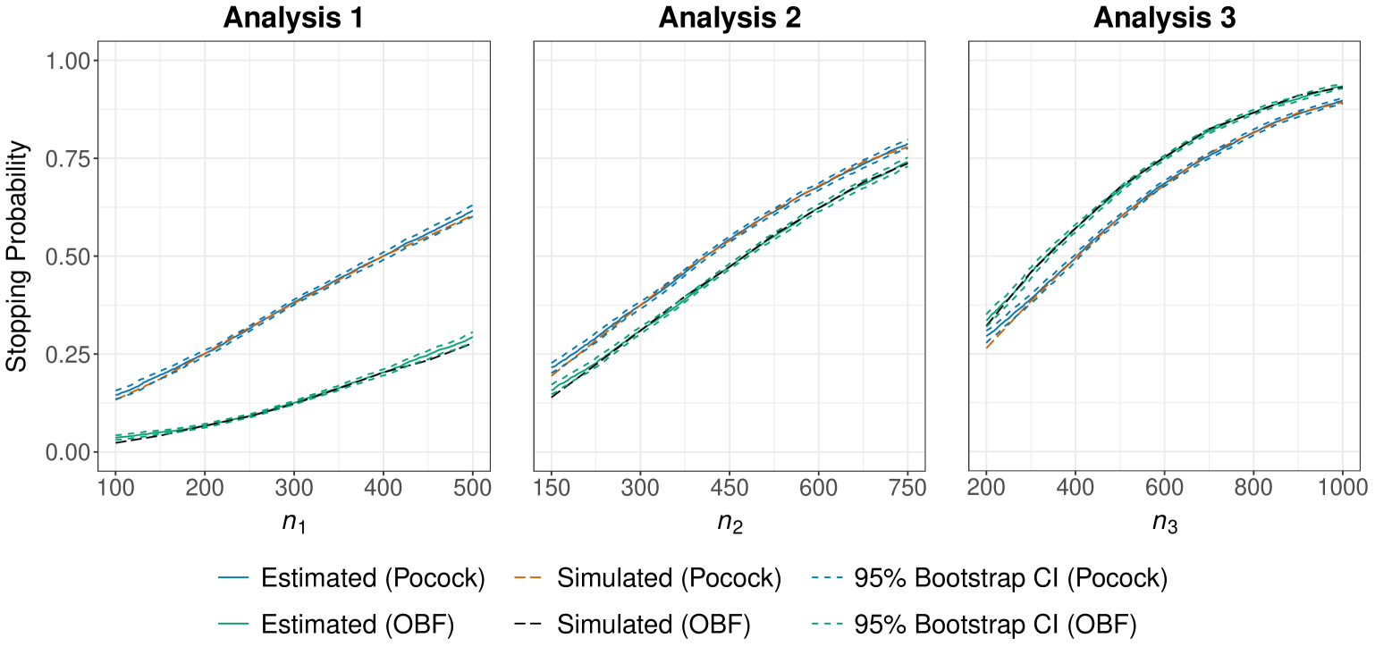
Figure 1: The cumulative stopping probabilities under $\Psi_{1}$ with a population-level rate ratio of 1.3. The solid curves are estimated using linear approximations. The short-dashed curves are pointwise 95% bootstrap confidence intervals. The long-dashed curves arise from simulating sampling distributions for many $n$ values.

Although the long-dashed curves are impacted by simulation variability, we use them as surrogates for the true stopping probabilities. We observe good alignment for all three analyses between the solid curves estimated using linear approximations and the long-dashed ones obtained by independently simulating samples. Apart from slight deviations at the smaller sample sizes in Figure 1, the long-dashed curves are generally contained within the pointwise 95% bootstrap confidence intervals. The agreement between the solid and long-dashed curves could be improved for smaller sample sizes if the linear approximations were calibrated using estimates of the sampling distribution at smaller sample sizes. We emphasize that the solid curves are substantially easier to obtain since we need only estimate the sampling distribution of $\boldsymbol{\tau}(\mathcal{D}_{n})$ at two values of $n$. Even so, it took roughly 35 minutes on a high-computing server to estimate each set of three solid curves in Figure 1 when approximating each posterior using Markov chain Monte Carlo with one chain where the first 1000 iterations were discarded as burnin and the next $3.2\times 10^{4}$ iterations were thinned, retaining every fourth draw. While initial simulations used multiple Markov chains to verify convergence, our large-scale simulations employed less intensive settings that achieved reasonable convergence. We considered 9 values of $n$ to simulate each set of three long-dashed curves in Figure 1, taking roughly 2.5 hours using the same computing resources. Unlike standard methods, our approach also allows practitioners to assess error rates for new values of $n$ without conducting additional simulations.

The numerical results for both boundary functions and all data generation processes $\Psi_{0}$ and $\Psi_{1}$ are summarized in Table 1. The first two rows for each scenario compare the cumulative stopping probabilities obtained using the linear approximations in Algorithm 1 with those obtained by estimating the joint sampling distribution of $\boldsymbol{\tau}(\mathcal{D}_{n})$ at $\{n_{1},n_{2},n_{3}\}=n\times\{1,1.5,2\}$, where non-integer sample sizes were rounded up to the nearest whole number. We observe good alignment between the first two rows for each scenario, demonstrating the strong performance of our method. The third row for each scenario confirms that the approximate Pocock and OBF decision thresholds bound the overall type I error rate in the final column by $\Gamma_{0}=0.025$.

				Cumulative Stopping Probability
Boundary	$n$	Rate Ratio	Method	00 $t=1$00	00 $t=2$ 00	00 $t=3$ 00
Pocock	386	1.3	Algorithm 1	0.4848	0.6628	0.8007
			Simulation	0.4938	0.6755	0.8140
		1	Simulation	0.0120	0.0165	0.0197
	223	1.4	Algorithm 1	0.4803	0.6583	0.8004
			Simulation	0.4893	0.6667	0.8047
		1	Simulation	0.0116	0.0163	0.0205
	161	1.5	Algorithm 1	0.4786	0.6611	0.8021
			Simulation	0.4942	0.6696	0.8055
		1	Simulation	0.0125	0.0174	0.0216
OBF	335	1.3	Algorithm 1	0.1523	0.5281	0.8002
			Simulation	0.1619	0.5405	0.8051
		1	Simulation	0.0015	0.0088	0.0219
	203	1.4	Algorithm 1	0.1472	0.5627	0.8018
			Simulation	0.1525	0.5424	0.8103
		1	Simulation	0.0010	0.0081	0.0203
	139	1.5	Algorithm 1	0.1393	0.5199	0.8013
			Simulation	0.1553	0.5389	0.8057
		1	Simulation	0.0011	0.0074	0.0205

Table 1: Stopping probabilities at the recommended $n$ values for the PLATINUM-CAN example obtained using linear approximations from Algorithm 1 and by simulating confirmatory estimates of sampling distributions.

5.2 Quality Control for Decaffeinated Coffee

We next assess the performance of our method with an example design based on quality control for decaffeinated coffee. The U.S. Department of Agriculture requires that decaffeinated coffee beans retain at most 3% of their initial caffeine content after the decaffeination process. In this example, we suppose that a coffee producer wants to perform quality control on a revamped decaffeination process. High-performance liquid chromatography (HPLC) is the gold-standard method to measure the caffeine content in coffee beans (Ashoor et al., 1983). Since there can be substantial variability in the caffeine content across different batches of decaffeinated coffee output from the same manufacturing process (McCusker et al., 2006), samples of coffee beans from a variety of batches must be tested. A sequential quality control experiment that allows early stopping for both success and failure would mitigate the costs of HPLC (Ashoor et al., 1983) and the risk of producing unsellable coffee batches.

The datum collected from each coffee batch is the proportion of caffeine remaining. Because these proportions are close to zero in acceptable decaffeinated coffee beans, the MLE’s stability and the suitability of the normal approximation to its sampling distribution may be questionable for small and moderate sample sizes. Bayesian analysis of the proportions is advantageous: it does not rely on asymptotic approximations to estimate posterior distributions and allows for the use of priors to improve stability when necessary. This example hence confirms the performance of our method with smaller sample sizes.

The proportions of residual caffeine obtained from the revamped decaffeination process are modeled using a beta distribution, parameterized by shape parameters $\boldsymbol{\theta}=(\alpha,\beta)$. The target of inference $\delta(\boldsymbol{\theta})$ is the 0.99-quantile of this distribution: $\delta=F^{-1}(0.99;\alpha,\beta)$, where $F^{-1}(\cdot)$ is the inverse CDF of the beta distribution. The hypotheses for this experiment are $H_{0}:\delta\geq 0.03$ vs. $H_{1}:\delta<0.03$. That is, we aim to conclude that the probability of producing an unsatisfactory batch of decaffeinated coffee beans is at most 0.01 using the interval endpoints $\delta_{L}=-\infty$ and $\delta_{U}=0.03$.

We design this experiment with $T=4$ analyses such that $c_{2}=1.5$, $c_{3}=2$, and $c_{4}=2.5$. We accommodate stopping for success based on posterior probabilities and stopping for failure based on posterior predictive probabilities. We want the cumulative type I error rate to be at most $\Gamma_{0}=0.1$ and power to be at least $\Gamma_{1}=0.8$. We do not have decision thresholds $\boldsymbol{\xi}$ or $\boldsymbol{\eta}$ for this example. For illustration, we use success thresholds $\boldsymbol{\gamma}=(0.9907,0.9691,0.9445,0.9211)$ from an alpha-spending function that approximates the OBF boundaries and failure thresholds $\boldsymbol{\xi}=(0.1,0.2,0.3)$. We later discuss why estimating the sampling distribution of $\boldsymbol{\tau}_{\hskip-1.25pt*}(\mathcal{D}_{n})$ under $\Psi_{0}$ in Line 2 of Algorithm 1 to obtain the success thresholds would be beneficial for this example.

To illustrate that the predictive and conditional approaches give rise to distinct sample size recommendations, we consider two $\Psi_{1}$ models. The predictive model $\Psi_{1}$ ensures that $\{\delta(\boldsymbol{\theta}_{r})\}_{r=1}^{R}\sim\mathcal{U}(0.0225,0.0275)$, and the conditional model $\Psi_{1}$ is such that $\delta(\boldsymbol{\theta}_{r})=0.025$ for all Monte Carlo iterations. Both $\Psi_{1}$ models are paired with a conditional $\Psi_{0}$ model that ensures $\delta(\boldsymbol{\theta}_{r})=0.03$ across all iterations. We elaborate on these choices for $\Psi_{1}$ and $\Psi_{0}$ and specify diffuse priors in Appendix D of the supplement. For both $\Psi_{1}$ models we consider, Algorithm 1 was implemented with $R=10^{4}$ and $M=10^{3}$ and an initial sample size for the first analysis of $n_{a}=18$. Under the predictive approach, the logits of posterior summaries were split into 10 subgroups based on the order statistics of their $\delta_{r}$ values before constructing the linear approximations. Based on the linear approximations in Algorithm 1, the recommended sample size for the initial analysis is $n=29$ under the predictive approach and $n=25$ under the conditional approach. 95% bootstrap confidence intervals for these optimal sample sizes $n$ obtained using our bootstrap procedure with $B=2000$ bootstrap samples were respectively $[28,30]$ and $[25,26]$.

It took roughly 15 hours on a high-computing server to implement Algorithm 1 for each $\Psi_{1}$ model when approximating each posterior using Markov chain Monte Carlo with one chain of 1000 burnin iterations and $5\times 10^{3}$ retained iterations. We again examined initial simulations with multiple Markov chains to verify convergence. Appendix D contains a plot similar to Figure 1 for this decaffeinated coffee example. We observed good alignment in that supplemental figure between our results based on linear approximations and those obtained by independently estimating the sampling distribution of $\boldsymbol{\tau}_{\hskip-1.25pt*}(\mathcal{D}_{n})$ at various $n$ values. It took roughly 2 days to obtain the results for each $\Psi_{1}$ model based on the various sampling distribution estimates using the same computing resources. Thus, estimating the sampling distribution of posterior summaries at only two values of $n$ greatly expedites the design process.

The numerical results for all data generation processes $\Psi_{0}$ and $\Psi_{1}$ are summarized in Table 2. The first two rows for each approach verify the alignment between the cumulative stopping probabilities obtained using the linear approximations in Algorithm 1 and those obtained by estimating the joint sampling distribution of $\boldsymbol{\tau}_{\hskip-1.25pt*}(\mathcal{D}_{n})$ at $\{n_{1},n_{2},n_{3},n_{4}\}=n\times\{1,1.5,2,2.5\}$. The third row for each approach demonstrates that we have a large cumulative probability of correctly stopping for failure when $H_{0}$ is true; however, the OBF success thresholds do not bound the overall type I error rate in the column with $t=4$ by 0.1. The OBF bounds fail for this example because the uniform approximation to the sampling distribution of $\boldsymbol{\tau}(\mathcal{D}_{n})$ is not accurate for small and moderate sample sizes – not because the quality of the linear approximations is poor. In Appendix D, we further explore these numerical results, verify the quality of the linear approximations for smaller sample sizes, and demonstrate that our method can be used to choose better values for $\boldsymbol{\gamma}$ and $n$ without conducting additional simulations.

				Cumulative Stopping Probability
				Success				Failure
Approach	$n$	Model	Method	$t=1$	$t=2$	$t=3$	$t=4$	$t=1$	$t=2$	$t=3$
Predictive	29	$\Psi_{1}$	Algorithm 1	0.2690	0.5483	0.7264	0.8033	0.0426	0.1073	0.1650
			Simulation	0.2594	0.5457	0.7267	0.8089	0.0392	0.0947	0.1486
		$\Psi_{0}$	Simulation	0.0356	0.0847	0.1342	0.1716	0.3326	0.6057	0.7564
Conditional	25	$\Psi_{1}$	Algorithm 1	0.2350	0.5153	0.7123	0.8000	0.0403	0.0977	0.1597
			Simulation	0.2404	0.5191	0.7147	0.8068	0.0391	0.0955	0.1508
		$\Psi_{0}$	Simulation	0.0363	0.0861	0.1443	0.1764	0.3232	0.5918	0.7504

Table 2: Stopping probabilities at the recommended $n$ values for the decaffeinated coffee example obtained using linear approximations from Algorithm 1 and by simulating confirmatory estimates of sampling distributions.

6 Discussion

In this paper, we proposed an economical framework to estimate error rates associated with decision procedures based on posterior and posterior predictive probabilities in sequential designs. This framework determines the minimum sample sizes that ensure the power of the experiment is sufficiently large while bounding the type I error rate. The computational efficiency of our framework is predicated on a proxy for the joint sampling distribution of posterior summaries across analyses. We use the behaviour in this large-sample proxy to motivate estimating true sampling distributions at only two sample sizes. Our method significantly reduces the computational overhead required to design Bayesian sequential experiments. We also repurposed our sampling distribution estimates to construct bootstrap confidence intervals that assess the impact of simulation variability on the sample size recommendations. Our methodology can be broadly used to design sequential experiments in a wide range of disciplines.

The methods proposed in this paper could be extended in various aspects to accommodate more complex sequential designs. Our work in this article constrained the sample sizes for the analyses to be such that $\{n_{t}\}_{t=1}^{T}=n\times\{1,c_{2},\dots,c_{T}\}$ as the sample size $n$ for the first analysis changes. This constraint precludes sequential designs that leverage response-adaptive randomization, including Thompson sampling (Thompson, 1933). Response-adaptive randomization is commonly incorporated into clinical trials and multi-armed bandit experiments (Katehakis and Veinott Jr, 1987) more generally. Furthermore, the posterior predictive probabilities we considered here did not account for potential stopping between the current and final analyses. Accounting for such stopping would more accurately reflect how sequential designs are implemented in practice, but this extension would increase the computational complexity of simulation-based sequential design. Future research could consider how to efficiently implement these extensions.

Moreover, the proxy sampling distributions introduced in this article rely on large-sample regularity conditions. The regularity conditions for the asymptotic normality of the MLE prevent us from considering designs with time-varying parameters. The conditions for the BvM theorem might also be violated if using certain methods to dynamically incorporate prior information into Bayesian sequential designs. The ability to dynamically incorporate such prior information could materially reduce the duration and cost of sequential experiments. We could further broaden the impact of our methods by relaxing some of these regularity conditions in future work.

Supplementary Material

These materials include the proofs of Lemma 1, Lemma 2, and Theorem 1, as well as additional content for our examples in Section 5. The code to conduct the numerical studies in the paper is available online: https://github.com/lmhagar/SeqDesign.

Funding Acknowledgement

Luke Hagar acknowledges the support of a postdoctoral fellowship from the Natural Sciences and Engineering Research Council of Canada (NSERC). Shirin Golchi acknowledges support from NSERC, Canadian Institute for Statistical Sciences (CANSSI), and Fonds de recherche du Québec - Santé (FRQS).

References

- Ashoor et al. (1983) Ashoor, S. H., G. J. Seperich, W. C. Monte, and J. Welty (1983). High performance liquid chromatographic determination of caffeine in decaffeinated coffee, tea, and beverage products. Journal of the Association of Official Analytical Chemists 66(3), 606–609.
- Berger-Tal et al. (2014) Berger-Tal, O., J. Nathan, E. Meron, and D. Saltz (2014). The exploration-exploitation dilemma: A multidisciplinary framework. PLOS One 9(4), e95693.
- Berry et al. (2010) Berry, S. M., B. P. Carlin, J. J. Lee, and P. Muller (2010). Bayesian adaptive methods for clinical trials. CRC press.
- De Santis (2007) De Santis, F. (2007). Using historical data for Bayesian sample size determination. Journal of the Royal Statistical Society: Series A (Statistics in Society) 170(1), 95–113.
- Demets and Lan (1994) Demets, D. L. and K. G. Lan (1994). Interim analysis: the alpha spending function approach. Statistics in Medicine 13(13-14), 1341–1352.
- Deng et al. (2024) Deng, A., L. Hagar, N. T. Stevens, T. Xifara, and A. Gandhi (2024). Metric decomposition in A/B tests. In Proceedings of the 30th ACM SIGKDD Conference on Knowledge Discovery and Data Mining, pp. 4885–4895.
- Deng et al. (2016) Deng, A., J. Lu, and S. Chen (2016). Continuous monitoring of A/B tests without pain: Optional stopping in Bayesian testing. In 2016 IEEE International Conference on Data Science and Advanced Analytics (DSAA), pp. 243–252. IEEE.
- Deng et al. (2022) Deng, C., A. Kim, and W. Lu (2022). A generic battery-cycling optimization framework with learned sampling and early stopping strategies. Patterns 3(7), 100531.
- Efron (1982) Efron, B. (1982). The Jackknife, the Bootstrap and Other Resampling Plans. SIAM.
- FDA (2019) FDA (2019). Adaptive designs for clinical trials of drugs and biologics — Guidance for industry. Center for Drug Evaluation and Research, U.S. Food and Drug Administration, Rockville, MD.
- Gelman et al. (1996) Gelman, A., X.-L. Meng, and H. Stern (1996). Posterior predictive assessment of model fitness via realized discrepancies. Statistica sinica, 733–760.
- Golchi (2022) Golchi, S. (2022). Estimating design operating characteristics in Bayesian adaptive clinical trials. Canadian Journal of Statistics 50(2), 417–436.
- Golchi and Willard (2024) Golchi, S. and J. J. Willard (2024). Estimating the sampling distribution of posterior decision summaries in Bayesian clinical trials. Biometrical Journal 66(8), e70002.
- Gubbiotti and De Santis (2011) Gubbiotti, S. and F. De Santis (2011). A Bayesian method for the choice of the sample size in equivalence trials. Australian & New Zealand Journal of Statistics 53(4), 443–460.
- Hagar and Golchi (2025) Hagar, L. and S. Golchi (2025). Design of Bayesian clinical trials with clustered data and multiple endpoints. arXiv preprint arXiv:2501.13218.
- Hagar and Stevens (2025) Hagar, L. and N. T. Stevens (2025). An economical approach to design posterior analyses. Journal of the American Statistical Association, doi.org/10.1080/01621459.2025.2476221.
- Halperin et al. (1982) Halperin, M., K. G. Lan, J. H. Ware, N. J. Johnson, and D. L. DeMets (1982). An aid to data monitoring in long-term clinical trials. Controlled Clinical Trials 3(4), 311–323.
- Jenkins and Peacock (2011) Jenkins, C. and J. Peacock (2011). The power of Bayesian evidence in astronomy. Monthly Notices of the Royal Astronomical Society 413(4), 2895–2905.
- Jennison and Turnbull (1999) Jennison, C. and B. W. Turnbull (1999). Group Sequential Methods with Applications to Clinical Trials. CRC Press.
- Katehakis and Veinott Jr (1987) Katehakis, M. N. and A. F. Veinott Jr (1987). The multi-armed bandit problem: Decomposition and computation. Mathematics of Operations Research 12(2), 262–268.
- Klein (2024) Klein, M. (2024). Tecovirimat in non-hospitalized patients with monkeypox (platinum-can). https://clinicaltrials.gov/study/NCT05534165.
- Lachin (2005) Lachin, J. M. (2005). A review of methods for futility stopping based on conditional power. Statistics in Medicine 24(18), 2747–2764.
- Lehmann and Casella (1998) Lehmann, E. L. and G. Casella (1998). Theory of Point Estimation. Springer Science & Business Media.
- McCusker et al. (2006) McCusker, R. R., B. Fuehrlein, B. A. Goldberger, M. S. Gold, and E. J. Cone (2006). Caffeine content of decaffeinated coffee. Journal of analytical toxicology 30(8), 611–613.
- O’Brien and Fleming (1979) O’Brien, P. C. and T. R. Fleming (1979). A multiple testing procedure for clinical trials. Biometrics, 549–556.
- Pocock (1977) Pocock, S. J. (1977). Group sequential methods in the design and analysis of clinical trials. Biometrika 64(2), 191–199.
- Ries et al. (2024) Ries, D., V. R. Sieck, P. Jones, and J. Shaffer (2024). Measuring the robustness of predictive probability for early stopping in two-group comparisons. Journal of Quality Technology 56(3), 276–289.
- Rubin (1984) Rubin, D. B. (1984). Bayesianly justifiable and relevant frequency calculations for the applied statistician. The Annals of Statistics, 1151–1172.
- Saville et al. (2014) Saville, B. R., J. T. Connor, G. D. Ayers, and J. Alvarez (2014). The utility of Bayesian predictive probabilities for interim monitoring of clinical trials. Clinical Trials 11(4), 485–493.
- Shi and Yin (2019) Shi, H. and G. Yin (2019). Control of type I error rates in Bayesian sequential designs. Bayesian Analysis 14(2), 399–425.
- Shiryaev (2007) Shiryaev, A. N. (2007). Optimal Stopping Rules, Volume 8. Springer Science & Business Media.
- Spiegelhalter et al. (2004) Spiegelhalter, D. J., K. R. Abrams, and J. P. Myles (2004). Bayesian Approaches to Clinical Trials and Healthcare Evaluation, Volume 13. John Wiley & Sons.
- Spiegelhalter et al. (1994) Spiegelhalter, D. J., L. S. Freedman, and M. K. Parmar (1994). Bayesian approaches to randomized trials. Journal of the Royal Statistical Society: Series A (Statistics in Society) 157(3), 357–387.
- Thompson (1933) Thompson, W. R. (1933). On the likelihood that one unknown probability exceeds another in view of the evidence of two samples. Biometrika 25(3-4), 285–294.
- van der Vaart (1998) van der Vaart, A. W. (1998). Asymptotic Statistics. Cambridge Series in Statistical and Probabilistic Mathematics. Cambridge University Press.
- Wald (2004) Wald, A. (2004). Sequential Analysis. Courier Corporation.
- Wang and Gelfand (2002) Wang, F. and A. E. Gelfand (2002). A simulation-based approach to Bayesian sample size determination for performance under a given model and for separating models. Statistical Science 17(2), 193–208.
- Wassmer and Brannath (2016) Wassmer, G. and W. Brannath (2016). Group Sequential and Confirmatory Adaptive Designs in Clinical Trials. Springer.