Integrating Fourier Neural Operators with Diffusion Models to improve Spectral Representation of Synthetic Earthquake Ground Motion Response

Abstract

Nuclear reactor buildings must be designed to withstand the dynamic load induced by strong ground motion earthquakes. For this reason, their structural behavior must be assessed in multiple realistic ground shaking scenarios (e.g., the Maximum Credible Earthquake). However, earthquake catalogs and recorded seismograms may not always be available in the region of interest. Therefore, synthetic earthquake ground motion is progressively being employed, although with some due precautions: earthquake physics is sometimes not well enough understood to be accurately reproduced with numerical tools, and the underlying epistemic uncertainties lead to prohibitive computational costs related to model calibration. In this study, we propose an AI physics-based approach to generate synthetic ground motion, based on the combination of a neural operator that approximates the elastodynamics Green’s operator in arbitrary source-geology setups, enhanced by a denoising diffusion probabilistic model. The diffusion model is trained to correct the ground motion time series generated by the neural operator. Our results show that such an approach promisingly enhances the realism of the generated synthetic seismograms, with frequency biases and Goodness-Of-Fit (GOF) scores being improved by the diffusion model. This indicates that the latter is capable to mitigate the mid-frequency spectral falloff observed in the time series generated by the neural operator. Our method showcases fast and cheap inference in different site and source conditions.

Keywords Earthquake simulation  $\cdot$ MIFNO  $\cdot$ DDPM

1 Introduction

Recent advances in high-performance computing (HPC) tools have enabled the numerical simulation of elastodynamic problems in complex setups. In this context, simulating large-scale earthquake scenarios, typically spanning urban regions ($\approx$100 km $\times$ 100 km $\times$ 50 km), requires high-resolution models with sub-meter accuracy, to match the Earth’s complex structure. Current state-of-the-art simulations can model active fault ruptures and wave propagation through complex geological structures, but they still face challenges in simulating high-frequency surface motions, limiting the fidelity of fault-to-structure and soil-structure interaction analyses [1]. These issues arise not only due to the inherent computational demand, but especially because of the uncertainties in subsurface properties [2] and seismogenetic source [3], making it difficult to generate broadband signals suitable for structural design.

The latter task of generating broadband (0-30 Hz) seismograms, is still far from being accomplished, either with empirical [4], or numerical approaches [5]. With the recent machine learning improvements, neural networks have been successfully applied to enhancing low-frequency seismograms with high-frequency content [6]. Among the developed methods, diffusion models [7] stand out due to their ease of training, performance, diversity of inferred samples, and the ability to use a variety of preexisting architectures as backbone generator. Diffusion models are increasingly being applied to generate realistic ground motion scenarios, conditioned on various metadata such as site and event characteristics (e.g., magnitude, source-to-site distance, and coordinates, [8], among others).

In this study, we present a novel deep learning strategy to yield multiple realistic strong-motion accelerograms in the 0-5 Hz frequency range, combining a physics-based surrogate model with a generative model. To this end, we employ the Multiple-Input Fourier Neural Operator (MIFNO) proposed by [9] in conjunction with the conditional diffusion architecture presented in [10]. The MIFNO acts as a fast surrogate model of 3D elastodynamics for arbitrary geological settings and source characteristics. We address MIFNO limitations in capturing mid-frequency details by employing a denoising diffusion probabilistic model [DDPM, 7] to improve the spectral content of the inferred wavefield at the free surface. Both the MIFNO and the DDPM are trained on elastodynamics simulations, the targets being the time-dependent wavefields for the MIFNO and the single-station seismograms for the DDPM. The results show that the combination of MIFNO and DDPM increases the realism of the rendered elastodynamic wavefield, by mitigating the MIFNO mid-frequency spectral bias. Our method preserves the fast inference of multiple earthquake scenarios (any geology, any source). The remainder of the paper is organized as follows: Section METHODS describes the key concepts behind MIFNO and DDPM. The results are discussed in Section RESULTS, and the conclusions are drawn in Section CONCLUSIONS.

2 Methods

2.1 Multiple-Input Fourier Neural Operator (MIFNO)

The 3D elastodynamics problem in a domain $\Omega\subset\mathbb{R}^{3}$ reads:

$$\mathcal{L}\left[\bm{a},\bm{v}\right](\bm{x},t)=\bm{f}[\bm{x_{s}},\bm{\theta_{s}}](\bm{x},t),\quad\forall(\bm{x},t)\in\Omega\times\left]0,T\right]$$ (1)

where $\mathcal{L}\left[\bm{a},\bm{v}\right]$ is the 3D elastic wave equation parametrized by the Lamé parameters $\bm{a}(\bm{x})$. $\bm{f}\in L^{2}(\Omega\times]0,T[,\mathbb{R}^{3})$ is the body force distribution, expressed as $\mathrm{div}~\>~\bm{m}(\bm{x})~\cdot~s(t)$, the divergence of a double-couple moment tensor density $\bm{m}\in H^{1}\left(\Omega\right)^{6}$, localized at a point-wise location $\bm{x_{s}}$ and with strike, dip, rake angles regrouped in vector $\bm{\theta_{s}}\in\mathbb{R}^{3}$. $s(t)\in C^{0}\left(\left]0,T\right]\right)$ represents the time-varying source amplitude over the duration $T$. Finally, $\bm{v}\in\mathcal{C}^{1}(\Omega\times]0,T[,\mathbb{R}^{3})$ is the particle velocity field, solution of the problem.

The MIFNO is a neural surrogate model $\mathbb{G}_{\bm{\phi}}:(\bm{a},\bm{x_{s}},\bm{\theta_{s}})\mapsto\bm{v}|_{\partial\Omega_{top}}$ of the Green’s operator, parametrized by weights $\bm{\phi}$, predicting the velocity field $\bm{v}$ at the Earth’s surface $\partial\Omega_{top}$, from the sole knowledge of the geology $\bm{a}$ and the source characteristics $\bm{x_{s}},\bm{\theta_{s}}$ . As shown in Figure 1, the MIFNO is fed with complex heterogeneous three-dimensional (3D) geological fields alongside data detailing earthquake point-source characteristics (position and moment tensor).

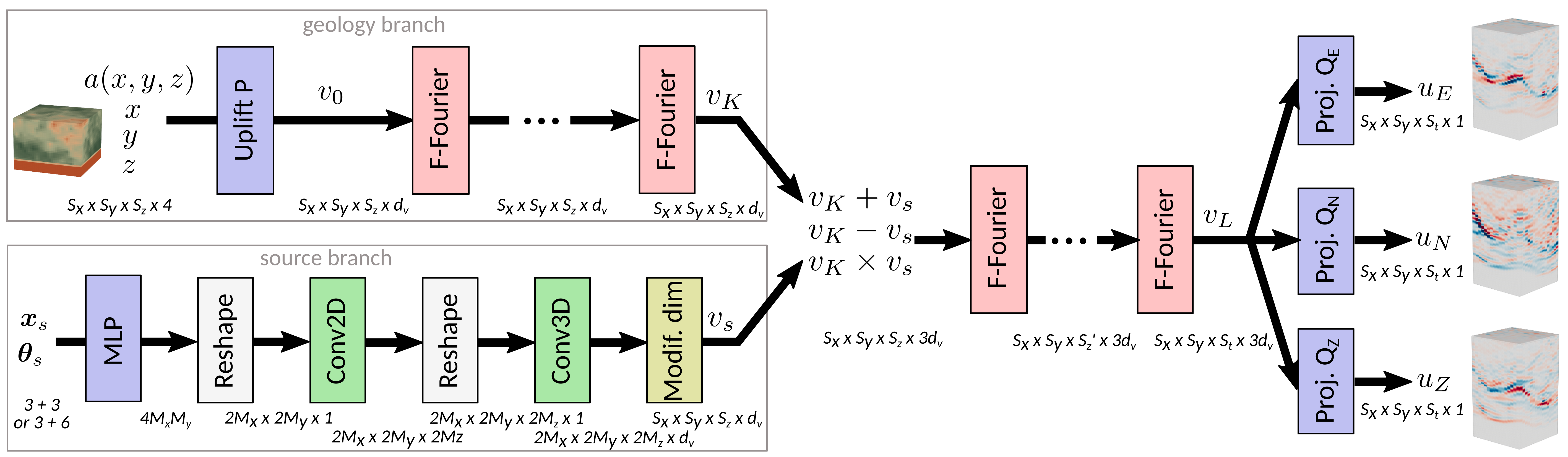
Figure 1: The MIFNO is made of a geology branch that encodes the geology with factorized Fourier (F-Fourier) layers, and a source branch that transforms the vector of source parameters $(\bm{x}_{s},\bm{\theta}_{s})$ into a 4D variable $v_{S}$ matching the dimensions of the geology branch output $v_{K}$. The outputs of each branch are concatenated after elementary mathematical operations and the remaining factorized Fourier layers are applied. Uplift $P$ and projection $Q_{E}$, $Q_{N}$, $Q_{Z}$ blocks are the same as in the F-FNO: they embed the geology field and project the latent space into the solution space, respectively. Reprinted from [9].

The MIFNO consists in a deep neural network of trainable weights $\bm{\phi}$, with two branches encoding the geology field $\bm{a}(\bm{x})$ and source characteristics $\bm{x}_{s}$, $\bm{\theta}_{s}$ respectively. The MIFNO backbone architecture is factorized Fourier (F-Fourier) layers [Factorized Fourier Neural Operator, F-FNO, proposed by 11]. Further details are provided in Figure 1. The MIFNO builds on the factorized Fourier Neural Operator (F-FNO, [11]) to learn the velocity field obtained with physics-based numerical simulations. The reference simulations were computed with the high-performance computing open-source software SEM3D [12], developed by the CEA, CentraleSupélec, CNRS and Institut de Physique du Globe de Paris. SEM3D demonstrated its ability to numerically reproduce high-fidelity fault-to-structure scenarios at regional scale (see, for instance [13, 14, 1]).

The MIFNO is trained with the open HEMEW${}^{\text{{S}}}$-3D database [15] to minimize the error between the predicted surface velocity fields $\bm{\hat{v}}$ and the simulated ones $\bm{v}$. HEMEW${}^{\text{{S}}}$-3D encompasses 30,000 SEM3D earthquake simulations, conducted in various heterogeneous geologies $\bm{a}(\bm{x})$, incorporating random source positions $\bm{x_{s}}$ and orientations $\bm{\theta_{s}}$ (see Figure 2). The HEMEW${}^{\text{{S}}}$-3D database is also the training database of the DDPM presented in this work.

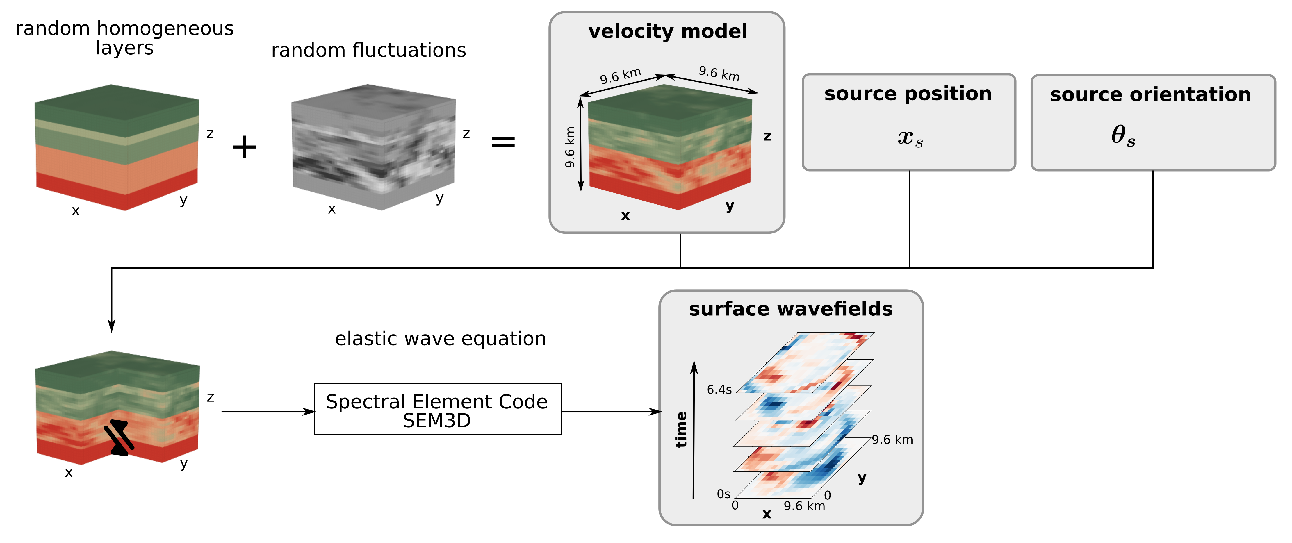
Figure 2: Composition of the HEMEW${}^{\text{{S}}}$-3D database. Velocity models were built from the addition of randomly chosen horizontal layers and heterogeneity drawn from random fields. Combined with the source position and the source orientation, they form the inputs of the neural operator. Outputs of the Spectral Element Code SEM3D are velocity wavefields synthesized at the surface of the domain by a grid of virtual sensors. Reprinted from [15].

[9] proved that the MIFNO yields accelerograms that score as good to excellent according to [16] Goodness-Of-Fit (GOF) metrics, compared to SEM3D reference signals. The accuracy of wave arrival times and the propagation of wave fronts is particularly notable, with 80% of the predictions achieving an outstanding phase GOF score greater than 8. Moreover, the amplitude fluctuations are deemed satisfactory for 87% of the predictions (with an envelope GOF exceeding 6) and are classified as excellent for 28% of cases. MIFNO demonstrates a commendable ability to generalize its predictions for sources located outside the training domain, and it exhibits solid generalization performance when applied to a real-world complex geological scenario characterized by overthrust formations. Additionally, when concentrating on specific regions of interest, transfer learning proves to be an effective strategy to enhance prediction accuracy without incurring significant costs. However, the prediction accuracy worsens when frequency increases. This is caused by the complex physical phenomena tied to high-frequency features and also reflects the well-known bias in neural networks, which states that small-scale features are more difficult to capture. This limitation can hamper the use of MIFNO in earthquake nuclear engineering applications.

2.2 Denoising Diffusion Probabilistic Model (DDPM)

Our DDPM is based on the original formulation by [7]. A DDPM exploits Markov Chain Monte Carlo sampling to generate realistic data (in our case, the 3-component seismograms $\bm{v}_{0}(t)\sim p_{data}$), starting from a sample drawn from the normal distribution $\bm{v}_{\mathcal{T}}(t)\sim\mathcal{N}(\mathbf{0},\mathbb{I})$. The Markov chain of a diffusion model consists of two discrete processes: the forward process, blurring the original data $\bm{v}_{0}(t)$ till reaching white noise, and the backward process, denoising the blurred data $\bm{v}_{\mathcal{T}}(t)$ to a new sample $\bm{\hat{v}}(t)$ that resembles the original data (see Figure 3).

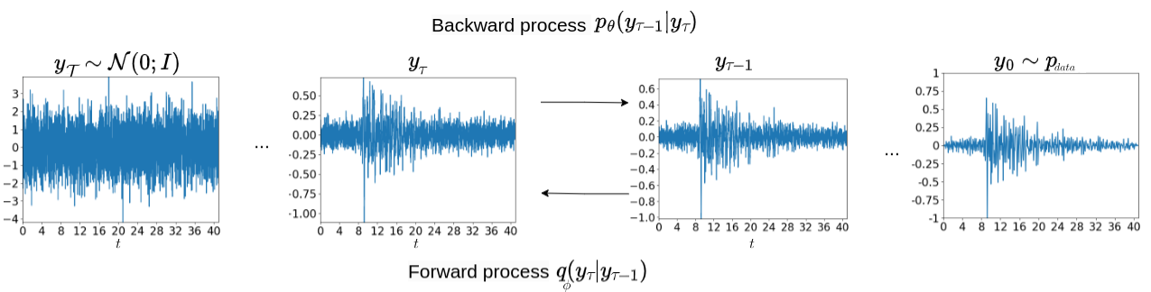
Figure 3: Diffusion process diagram. The forward process is associated to a transition kernel $q_{\phi}(\bm{v}_{\tau}|\bm{v}_{\tau-1})$, whereas the backward diffusion process is associated to the transition kernel $p_{\theta}(\bm{v}_{\tau}|\bm{v}_{\tau+1})$.

$\mathcal{T}$ is the duration of the diffusion process (typically, $\mathcal{T}=1000$ steps). The forward process consists of generating samples $(\bm{v}_{\tau})_{\tau=1}^{\mathcal{T}}$ with a Gaussian transition probability $q_{\phi}$ that reads:

$$q_{\phi}(\bm{v}_{\tau}|\bm{v}_{\tau-1}):=\mathcal{N}\left(\bm{v}_{\tau};\bm{v}_{\tau-1}\sqrt{1-\beta_{\tau}},\beta_{\tau}\mathbb{I}\right),\quad q(\bm{v}_{\tau}|\bm{v}_{0}):=\mathcal{N}\left(\bm{v}_{\tau};\sqrt{\bar{\alpha}_{\tau}}\bm{v}_{0},(1-\bar{\alpha}_{\tau})\mathbb{I}\right)$$ (2)

where $\alpha_{\tau}=1-\beta_{\tau}$ and $\bar{\alpha}_{\tau}=\prod_{s=1}^{\tau}\alpha_{s}$. The sequence $(\bm{v}_{\tau})_{\tau=1}^{\mathcal{T}}$ is generated by progressively adding Gaussian noise to an initial time series $\bm{v}_{0}$ selected from the available dataset. A noise variance $(\beta_{\tau})_{\tau=1}^{\mathcal{T}}$ is predefined by linearly increasing $\beta_{\tau}$ from 0.0001 to 0.02 [7]. The backward process is defined as the inverse of the forward process and allows for the approximation of $\bm{v}_{0}$ starting from $\bm{v}_{\mathcal{T}}\sim p_{\theta}(\bm{v}_{\mathcal{T}})=\mathcal{N}(\bm{y}_{\tau};\bm{0},\mathbb{I})$. The reverse process estimates $\bm{v}_{0}$ by maximizing the likelihood $p_{\theta}(\bm{v}_{0}|\bm{v}_{\mathcal{T}})$, defined as the product of transition probabilities:

$$p_{\theta}(\bm{v}_{\tau-1}|\bm{v}_{\tau}):=\mathcal{N}\left(\bm{v}_{t-1};\mu_{\theta}(\bm{v}_{\tau},\tau),\sigma_{\tau}^{2}\mathbb{I}\right),\quad p_{\theta}(\bm{v}_{0}|\bm{v}_{\mathcal{T}}):=p(\bm{v}_{\mathcal{T}})\prod_{\tau=1}^{\mathcal{T}}p_{\theta}(\bm{v}_{\tau-1}|\bm{v}_{\tau})$$ (3)

where $\mu_{\theta}(\bm{v}_{\tau},\tau)$ and $\sigma_{\tau}^{2}$ are the mean and variance estimated by the model for $\bm{v}_{\tau-1}$.

In practice, a neural network $\bm{\varepsilon_{\theta}}$ is used to parametrize $p_{\theta}(\bm{v}_{\tau-1}|\bm{v}_{\tau})$. This network infers the Gaussian noise $\bm{\varepsilon_{\theta}}(\bm{v}_{\tau},\tau)$ required to obtain $\bm{v}_{\tau-1}$ from $\bm{y}_{\tau}$, according to the following expression [7]:

$$\bm{v}_{t-1}=\frac{1}{\sqrt{\alpha_{\tau}}}\left(\bm{v}_{\tau}-\frac{1-\alpha_{\tau}}{\sqrt{1-\bar{\alpha}_{\tau}}}\bm{\varepsilon_{\theta}}(\bm{v}_{\tau},t)\right)+\sqrt{\beta_{\tau}}\bm{z}_{\tau},\quad\bm{z}_{\tau}\sim\mathcal{N}(\bm{0},\mathbb{I}).$$ (4)

The term $\bm{\varepsilon_{\theta}}(\bm{v}_{\tau},\tau)$ represents the estimation of the noise level contained in $\bm{v}_{\tau}$ at time step $\tau$. The challenge of diffusion models is thus to estimate the noise generated by the forward process, thereby enabling the recovery of $\bm{v}_{0}$ from $\bm{v}_{\mathcal{T}}$. The DDPM neural network $\bm{\varepsilon_{\theta}}$ ($\bm{\theta}$ represent the neural network trainable weights) is trained to minimize the following loss:

$$\mathit{L}(\bm{\theta})=\mathbb{E}_{\tau\sim\mathcal{U}([1,\mathcal{T}]),\bm{v}_{0}\sim p_{data},\bm{\varepsilon}_{\tau}\sim\mathcal{N}(\bm{0},\mathbb{I})}\left[\|\bm{\varepsilon}_{\tau}-\bm{\varepsilon_{\theta}}\left(\sqrt{\bar{\alpha_{\tau}}}\bm{v}_{0}+\sqrt{1-\bar{\alpha_{\tau}}}\bm{\varepsilon};\tau\right)\|^{2}\right]$$ (5)

In other words, $\bm{\varepsilon_{\theta}}$ plays the role of a denoiser that progressively transforms the noisy samples $\bm{v}_{\tau}$ into cleaner samples $\bm{v}_{\tau-1}$, by matching the estimated white noise added by the forward process. [10] adopted a UNet as the $\bm{\varepsilon_{\theta}}$ denoiser of 3-component accelerograms. This DDPM was trained to generate broadband (0-30Hz) signals, while being conditioned on the low-pass filtered signals (0-1Hz). In this manner, $\bm{\varepsilon_{\theta}}$ learns to conditionally denoise a white noise sample, being forced to match the conditioning input at low-frequency.

2.3 Enhancing MIFNO with DDPM

Our study takes inspiration from [17], who combine diffusion models and neural operators to enhance the resolution of turbulent structures. In the present work, the MIFNO predicts the ground motion velocity signals that serve as the conditioning of the DDPM. Since the low-frequency parts of the MIFNO predictions were shown to be close to the reference simulations [9], we argue that they contain relevant physical information to guide the diffusion process. It is important to note that the MIFNO is frozen in this work (i.e., its weights are not updated). The DDPM is trained to generate velocity time series from the HEMEW${}^{\text{{S}}}$-3D database, conditioned on the corresponding velocity prediction by the MIFNO (Fig. 4).

,

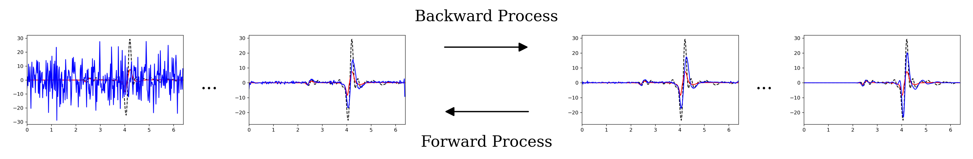
Figure 4: Forward and backward diffusion process conditioned by the MIFNO output (red). The SEM3D numerical solution, representing the target, is shown in black, while the DDPM output is shown in blue.

Our MIFNO+DDPM is trained on 19,200 realizations from the HEMEW${}^{\text{{S}}}$-3D database. From each realization, 32 sensors are randomly selected to obtain the 3-component velocity time series. This leads to 614,400 3-component velocity time series of duration 6.4s to train the MIFNO+DDPM. Training is done for 100 epochs, with a batch size 256, which took 13.29h on four A100 GPUs. A cosine annealing learning rate scheduler was used with 10 restarts, each cycle starting with learning rate 3e-4 and ending with 0.

At inference time, one entire wavefield prediction takes around 50ms and it can be enhanced with DDPM on 512 sensors at once in 3 minutes on one A100 GPU.

3 Results

Figure 5 (a-c) illustrates that the velocity time series obtained with MIFNO + DDPM (blue line) is closer to the reference simulation (black dashed line) than the original MIFNO prediction (red line). This shows that enhancing the surrogate model with the diffusion process improves the accuracy of the predictions. It is important to observe that the enhanced time series preserve the wave arrivals that were correctly predicted by the MIFNO. This indicates that the MIFNO conditioning is effective in transmitting the physical information of the signal and that the DDPM preserve this information.

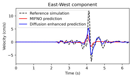
(a)

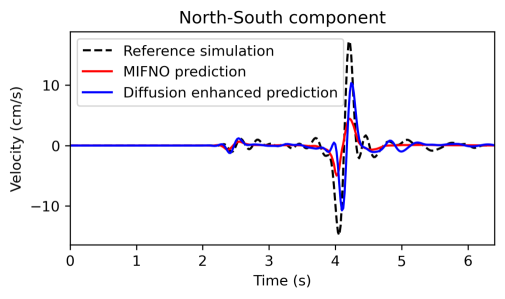
(b)

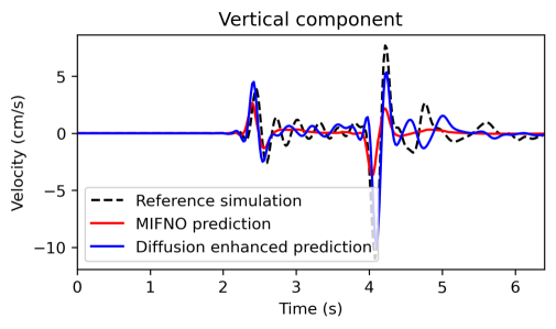
(c)

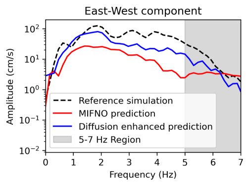
(d)

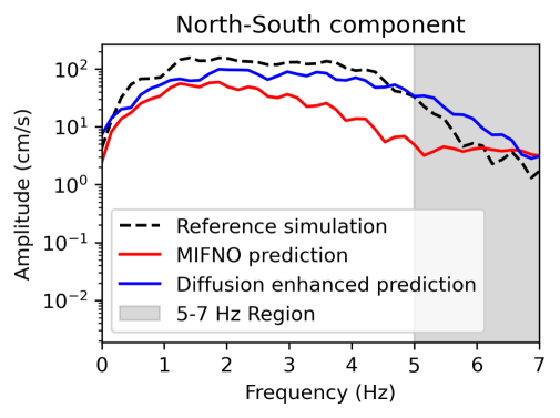
(e)

(f)

Figure 5: Comparison between the reference numerical simulation (black dashed line), the MIFNO prediction acting as conditioning (red line), and the signal enhanced by DDPM (blue line). The top panels (a, b, c) show the 3-component synthetic seismograms, while the bottom panels (d, e, f) show the corresponding spectra.

When looking at the spectral representations in Fig. 5 (d-f), one can observe that the DDPM improves the agreement between the predictions and the reference simulations in the entire frequency range, thereby mitigating the spectral bias of MIFNO.

Table 1: Accuracy metrics of the original MIFNO (first line) and MIFNO enhanced by DDPM (second line). 3000 test samples are compared with the reference simulations. The best metrics are indicated in bold. rMAE = relative Mean Absolute Error, rRMSE = relative Root Mean Square Error, rFFT = bias in Fourier coefficients between 0 and 1 Hz (low), 1 and 2 Hz (mid), 2 and 5 Hz (high), EG = Envelope GOF, PG = Phase GOF. More details on the metrics can be found in [18].

Metric	MIFNO	MIFNO + DDPM
rMAE	0.16 $\pm$ 0.06	0.20 $\pm$ 0.09
rRMSE	0.30 $\pm$ 0.11	0.34 $\pm$ 0.18
rFFTlow	-0.27 $\pm$ 0.19	0.04 $\pm$ 0.32
rFFTmid	-0.36 $\pm$ 0.23	0.08 $\pm$ 0.45
rFFThigh	-0.44 $\pm$ 0.27	0.11 $\pm$ 0.60
EG	6.15 $\pm$ 1.00	6.16 $\pm$ 1.12
PG	6.65 $\pm$ 1.07	7.52 $\pm$ 1.08

These visual observations are corroborated by the metrics computed on 3000 test samples. The MIFNO + DDPM preserves the physical consistency of the MIFNO since the enveloppe and phase GOF (resp. EG and PG) are better than the MIFNO. The improvement is especially visible on the phase GOF. These results are further illustrated in Fig. 6 where the large majority of points lie above the diagonal.

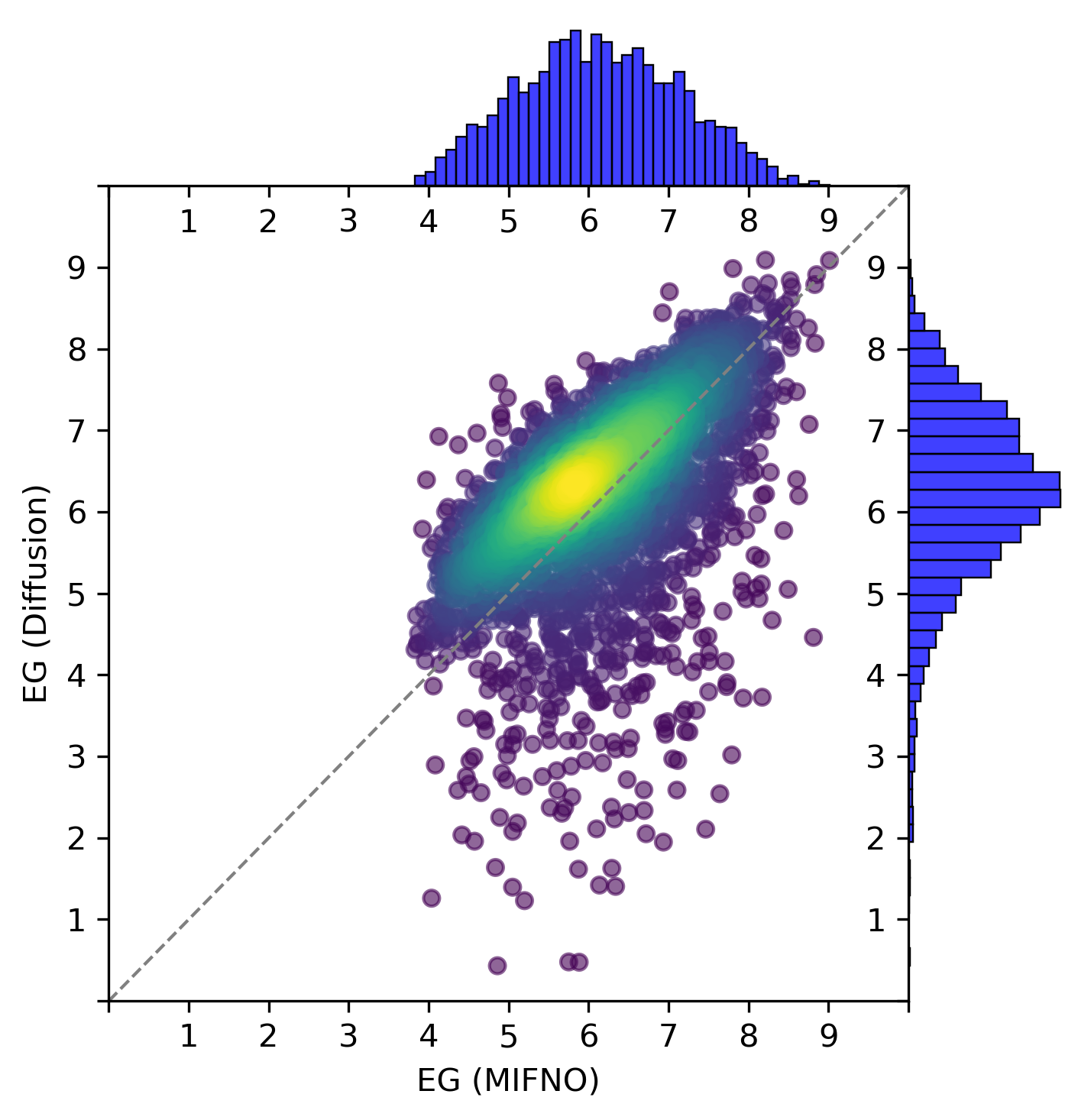
(a)

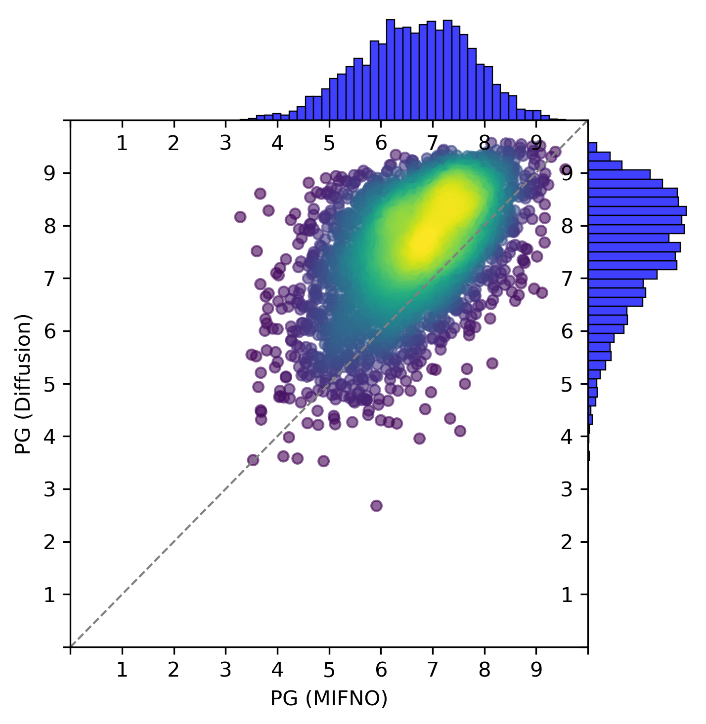
(b)

Figure 6: GOF scores (from 0 to 10, 10 being a perfect agreement) comparing the reference numerical simulation with the MIFNO (horizontal axis) and MIFNO + DDPM (vertical axis). (a) Envelope GOF; (b) Phase GOF. All time series were low-pass filtered in the 0-5 Hz frequency range for all the three components. The GOF score represents the average GOF across the three components. The color in the scatter plot shows the points density.

The DDPM corrects the MIFNO pre-conditioning across the entire 0-5 Hz frequency range as it reduces the frequency biases (in absolute value) given in Tab. 1. One can however notice that the relative MAE and RMSE are slightly higher for the MIFNO + DDPM than for the MIFNO. This can be related to some residual noise that affects these point-wise metrics while the physically-based metrics (i.e., frequency biases and GOF) are not sensitive to these small errors.

Figure 6 also indicates some samples where the diffusion model degrades the envelope GOF. This happens in most cases when the MIFNO amplitude is very small and the DDPM is not able to extract enough physical information from the MIFNO conditioning.

4 Discussion and Conclusions

In this paper, we foreshadowed the appealing perspective of combining neural operators and diffusion models in computational earthquake engineering. This strategy addresses an open challenge in this domain: the need for a fast earthquake simulator which is also accurate enough in the high-frequency range to be employed to design critical infrastructures. We combined the fast inference of the physics-based MIFNO surrogate model with the high-frequency accuracy of the DDPM generative model. This combination improves the accuracy of the synthetic seismograms while preserving the physical features learned by the MIFNO.

However, as per now, it must be noted that the seismograms generated by our MIFNO + DDPM are not yet accurate enough for practical applications. One possible explanation is that the DDPM treats the seismograms from the same realization (i.e., same source and same geology but observed at two different sensors) independently. Therefore, the spatial correlation between them is neglected. Explicitly introducing such correlation, acknowledging the difference among within- and between-event realizations, would steer the DDPM towards learning complex spatio-temporal patterns. Further work is required to extend the current DDPM architecture.

Nevertheless, from a practical perspective, the advantage of our proposed strategy lies in the possibility of quickly inferring approximate earthquake ground motion regional response, for any geology and any source, without running expensive numerical simulations. Moreover, the residual gap in accuracy presumably lies within the epistemic uncertainty margins of 0-5 Hz numerical simulations compared to recorded seismograms. With this tool at hand, we make progress towards unlocking physics-based probabilistic seismic hazard assessment. We envision the possibility of relegating cumbersome yet accurate earthquake numerical simulations to offline database enrichment, adopted to progressively fine-tune our MIFNO+DDPM surrogate model. The repercussions on the design procedures of nuclear facilities are potentially disruptive.

References

- [1] Reine Fares, David Castro Cruz, Evelyne Foerster, Fernando Lopez-Caballero, and Filippo Gatti. Coupling spectral and finite element methods for 3d physic-based seismic analysis from fault to structure: Application to the cadarache site in france. Nuclear Engineering and Design, 397:111954, October 2022.
- [2] David Castro-Cruz, Filippo Gatti, and Fernando Lopez-Caballero. High-fidelity broadband prediction of regional seismic response: a hybrid coupling of physics-based synthetic simulation and empirical green functions. Natural Hazards, 108(2):1997–2031, September 2021.
- [3] Kai Nakao, Tsuyoshi Ichimura, Kohei Fujita, Takane Hori, Tomokazu Kobayashi, and Hiroshi Munekane. Massively parallel bayesian estimation with sequential monte carlo sampling for simultaneous estimation of earthquake fault geometry and slip distribution. Journal of Computational Science, 81:102372, September 2024.
- [4] Nicolas M. Kuehn, Kenneth W. Campbell, and Yousef Bozorgnia. Potential biases in mixed-effects ground-motion models and variance components due to uncertainty in random effects. Bulletin of the Seismological Society of America, February 2025.
- [5] R. W. Graves and A. Pitarka. Broadband ground-motion simulation using a hybrid approach. Bulletin of the Seismological Society of America, 100(5A):2095–2123, October 2010. tex.eprint: http://www.bssaonline.org/content/100/5A/2095.full.pdf+html tex.owner: filippo tex.timestamp: 2017.07.05.
- [6] Manuel A. Florez, Michaelangelo Caporale, Pakpoom Buabthong, Zachary E. Ross, Domniki Asimaki, and Men-Andrin Meier. Data-driven synthesis of broadband earthquake ground motions using artificial intelligence. Bulletin of the Seismological Society of America, 112(4):1979–1996, 2022. SISMO.
- [7] Jonathan Ho, Ajay Jain, and Pieter Abbeel. Denoising Diffusion Probabilistic Models, December 2020.
- [8] Andreas Bergmeister, Kadek Hendrawan Palgunadi, Andrea Bosisio, Laura Ermert, Maria Koroni, Nathanaël Perraudin, Simon Dirmeier, and Men-Andrin Meier. High resolution seismic waveform generation using denoising diffusion, October 2024. arXiv:2410.19343 [physics].
- [9] Fanny Lehmann, Filippo Gatti, and Didier Clouteau. Multiple-input fourier neural operator (mifno) for source-dependent 3d elastodynamics. Journal of Computational Physics, 527:113813, April 2025.
- [10] Hugo Gabrielidis, Filippo Gatti, Stéphane Vialle, and Gottfried Jacquet. Génération conditionnelle et inconditionnelle de signaux sismiques à l’aide de modèles de diffusion. In 16ème Colloque National en Calcul des Structures, pages 1–9, Giens (VAR), France, 2024. Computational Structural Mechanics Association.
- [11] Alasdair Tran, Alexander Mathews, Lexing Xie, and Cheng Soon Ong. Factorized fourier neural operators, March 2023.
- [12] CEA, CentraleSupélec, IPGP, and CNRS. Sem3d ver 2017.04 registered at french agency for protection of programs (dépôt app), 2017.
- [13] Sara Touhami, Filippo Gatti, Fernando Lopez-Caballero, Régis Cottereau, Lúcio de Abreu Corrêa, Ludovic Aubry, and Didier Clouteau. SEM3D: A 3D High-Fidelity Numerical Earthquake Simulator for Broadband (0–10 Hz) Seismic Response Prediction at a Regional Scale. Geosciences, 12(3):112, March 2022.
- [14] D Castro-Cruz, F Gatti, F Lopez-Caballero, F Hollender, E El-Haber, and M Causse. Blind broad-band (0-10 hz) numerical prediction of the 3-d near field seismic response of an mw6.0 extended fault scenario: application to the nuclear site of cadarache (france). Geophysical Journal International, 232(1):581–600, October 2022.
- [15] F. Lehmann, F. Gatti, M. Bertin, and D. Clouteau. Synthetic ground motions in heterogeneous geologies from various sources: the HEMEW\textsuperscript{S}-3D database. Earth System Science Data, 16(9):3949–3972, 2024.
- [16] M. Kristekova, J. Kristek, and P. Moczo. Time-frequency misfit and goodness-of-fit criteria for quantitative comparison of time signals. Geophysical Journal International, 178(2):813–825, August 2009. tex.optissn: 1365-246X.
- [17] Vivek Oommen, Aniruddha Bora, Zhen Zhang, and George Em Karniadakis. Integrating neural operators with diffusion models improves spectral representation in turbulence modelling. Proceedings of the Royal Society A: Mathematical, Physical and Engineering Sciences, 481(2309):20240819, 2025.
- [18] Fanny Lehmann, Filippo Gatti, Michaël Bertin, and Didier Clouteau. 3d elastic wave propagation with a factorized fourier neural operator (f-FNO). Computer Methods in Applied Mechanics and Engineering, 420:116718, 2024.