Entanglement and Optimal Timing in Discriminating Quantum Dynamical Processes

Abstract

I address the problem of optimally discriminating between two open quantum dynamical processes. This problem is solved by identifying the optimal time at which two quantum channels, drawn from distinct sets of time-dependent channels, can be distinguished with minimal error probability, along with the optimal (potentially entangled) input state. I illustrate the richness of the solutions through an explicit study of Pauli dynamical maps and their corresponding sets of Pauli channels. Notably, I identify a scenario in which optimal discrimination without entanglement requires waiting indefinitely—i.e., until the unknown process reaches its stationary state—whereas the presence of entanglement allows for discrimination at a finite optimal time, along with a strict improvement in distinguishability.

Discriminating between different hypotheses is a fundamental task in both the foundations and applications of quantum information. Originally formulated by Helstrom hel in terms of minimizing error probability in quantum state discrimination, this problem has been extensively studied in various forms unam ; walg ; rev12 ; qifr and extended to the discrimination of unitary transformations CPR and quantum channels qi1 ; qi2 ; chiri . In the case of minimum-error discrimination between two quantum channels, entangled input states can provide a strict advantage, improving discrimination even in highly noisy scenarios, such as entanglement-breaking channels qi2 . This remarkable result has motivated significant research into quantum illumination protocols illu , where entangled states of light are used to enhance the detection of a faint signal amidst noise.

In this paper, I investigate the problem of optimally discriminating between two open quantum dynamical processes, focusing on the interplay between entanglement and timing in minimizing error probability. Specifically, I formulate the problem as identifying the optimal time at which two time-dependent quantum channels, each associated with a different open quantum dynamics, can be distinguished with the highest probability of success. This task requires not only determining the optimal measurement strategy but also identifying the optimal input state, which may be entangled, to maximize the distinguishability of the dynamical processes. The present study offers deep insights into the role of entanglement as a resource in quantum hypothesis testing and reveals the intricate relationship between temporal dynamics and distinguishability.

I show the richness of the solutions through the explicit study of Pauli dynamical maps and their corresponding sets of time-dependent Pauli channels. Pauli channels, which model noise processes in qubit systems, provide a simple yet physically relevant framework for exploring this discrimination problem qiP ; qif . Through this analysis, I uncover scenarios in which optimal discrimination without entanglement requires waiting indefinitely, until the unknown process reaches its stationary state. In contrast, the use of entangled input states enables discrimination at a finite optimal time, along with a strict reduction in error probability. This result underscores the crucial role of entanglement and proper timing in enhancing the distinguishability of quantum dynamical processes.

In general, a quantum dynamical process is governed by a generator ${\cal L}_{t}$ which dictates the evolution of the system quantum state $\rho(t)$ through the equation $\partial_{t}\rho(t)={\cal L}_{t}\rho(t)$. Under appropriate conditions, the superoperator ${\cal L}_{t}$ can take a particularly simple form as, for example, ${\cal L}_{t}=-i[H_{t},\cdot]$ for Hamiltonian dynamics, or a GKSL-like form for Markovian divisible evolution pb . Anyway, to represent a physically valid evolution, at any time $t$ the map ${\cal E}_{t}={\cal T}\exp(\int_{0}^{t}{\cal L}_{s}ds)$, defined via a time-ordered exponential of ${\cal L}_{t}$, must be a quantum channel—i.e. a trace-preserving completely positive map pb . In fact, this map ${\cal E}_{t}$ provides the quantum state $\rho(t)$ at time $t$ from any initial state $\rho(0)$ as $\rho(t)={\cal E}_{t}(\rho(0))$.

Now, suppose the system evolution is known to be governed by one of two possible dynamical processes, with generators ${\cal L}_{t}^{(1)}$ and ${\cal L}_{t}^{(2)}$, occurring with prior probabilities $q_{1}$ and $q_{2}=1-q_{1}$, respectively. The problem of distinguishing between these two evolutions reduce to finding the optimal time $t^{*}$ at which a discrimination test between the corresponding quantum channels ${\cal E}^{(1)}_{t}$ and ${\cal E}_{t}^{(2)}$ achieves the minimum error probability, potentially leveraging entangled input states.

I briefly recall from Ref. qi1 the main results on the general problem of minimum error discrimination between two generic quantum channels ${\cal E}^{(1)}$ and ${\cal E}^{(2)}$ given with prior probabilities $q_{1}$ and $q_{2}$. This problem is formulated by seeking the optimal input state $\rho$ for the Hilbert space $\cal H$ such that the error probability in discriminating the output states ${\cal E}^{(1)}(\rho)$ and ${\cal E}^{(2)}(\rho)$ is minimal. If side entanglement is allowed, the output states to be distinguished take the form $({\cal E}^{(1)}\otimes{\cal I})\rho$ and $({\cal E}^{(2)}\otimes{\cal I})\rho$, where the input $\rho$ is generally a bipartite state for ${\cal H}\otimes{\cal K}$, and the quantum channels act solely just on the first subsystem, while the identity map ${\cal I}$ acts on the second. Notably, the use of entanglement can strictly enhance discrimination, even in highly noisy scenarios qi2 .

Let me recall the result of Helstrom hel : the minimum error probability $p^{\prime}_{E}$ in the optimal discrimination between two quantum states $\rho_{1}$ and $\rho_{2}$, given with prior probabilities $q_{1}$ and $q_{2}=1-q_{1}$, is given by

$$p^{\prime}_{E}=\left(1-\|q_{1}\rho_{1}-q_{2}\rho_{2}\|_{1}\right)/2\;,$$ (1)

where $\|A\|_{1}=\hbox{Tr}\sqrt{A^{\dagger}A}$ denotes the trace norm of $A$. This result inherently accounts for the corresponding optimal (binary and orthogonal) measurement.

Then, for the case of channel discrimination without entanglement, the minimum error probability $\tilde{p}_{E}$ is given by

$$\tilde{p}_{E}=(1-\max_{\rho}\|q_{1}{\cal E}^{(1)}(\rho)-q_{2}{\cal E}^{(2)}(\rho)\|_{1})/2\,,$$ (2)

where $\rho$ is a density matrix for $\cal H$. On the other hand, when entanglement is permitted, the minimum error probability $p_{E}$ is given by

$$p_{E}=(1-\max_{\rho}\|q_{1}({\cal E}^{(1)}\otimes{\cal I})\rho-q_{2}({\cal E}^{(1)}\otimes{\cal I})\rho\|_{1})/2\,,$$ (3)

where $\rho$ is a density matrix for ${\cal H}\otimes{\cal K}$. The maximum of the trace norm in Eq. (3) is known as the norm of complete boundedness (or diamond norm). In fact, for finite-dimensional Hilbert space, one can simply take ${\cal K}={\cal H}$ paulsen ; diam . Moreover, due to the convexity of the trace norm, in both Eqs. (2) and (3) the maximum can be searched for among pure states.

It follows that the error probabilities in discriminating between the two dynamical maps ${\cal L}_{t}^{(1)}$ and ${\cal L}_{t}^{(2)}$ at time $t$ can be obtained from Eqs. (2) and (3) by replacing ${\cal E}^{(i)}$ with ${\cal E}_{t}^{(i)}={\cal T}\exp(\int_{0}^{t}{\cal L}^{(i)}_{s}ds)$. In this way, I promote $p_{E}$ (and $\tilde{p}_{E}$) to time dependent functions, whose infimum over $t>0$ provides the ultimate minimum error probability $p_{E}^{*}$ (and $\tilde{p}_{E}^{*}$) for discriminating between the dynamical maps, with (and without) use of side entanglement. I remark that when both dynamical processes are Hamiltonian, i.e. ${\cal L}^{(i)}_{t}=-i[H^{(i)}_{t},\cdot]$, entanglement never improves discrimination, since the two corresponding channels ${\cal E}_{t}^{(i)}$ are unitary CPR .

Now, I consider the explicit case of two Pauli dynamical maps for qubits, namely

$$\partial_{t}\rho(t)={\cal L}^{(i)}\rho(t)=\sum_{k=1}^{3}\gamma^{(i)}_{k}[\sigma_{k}\rho(t)\sigma_{k}-\rho(t)]\;.$$ (4)

where $\{\sigma_{1}\,,\sigma_{2}\,,\sigma_{3}\}=\{\sigma_{x}\,,\sigma_{y}\,,\sigma_{z}\}$ denote the Pauli matrices, and $\bm{\gamma}^{(i)}\equiv\{\gamma^{(i)}_{x}\,,\gamma^{(i)}_{y}\,,\gamma^{(i)}_{z}\}$ represent the vector of the pertaining decay rates. These maps are purely dissipative, have time-independent generators, and describe two distinct semi-group Markovian dynamics. The solutions ${\cal E}_{t}^{(i)}=e^{{\cal L}^{(i)}t}$ of Eq. (4) define two sets of Pauli channels ${\cal E}_{t}^{(1)}$ and ${\cal E}_{t}^{(2)}$, namely

$$\rho^{(i)}(t)={\cal E}_{t}^{(i)}(\rho(0))=\sum_{k=0}^{3}p_{k}^{(i)}(t)\sigma_{k}\rho(0)\sigma_{k}\;,$$ (5)

where I introduced $\sigma_{0}\equiv I$ as the $2\times 2$ identity matrix, along with the two time-dependent probability vectors $\{p^{(i)}_{k}(t)\}$. These probabilities are related to the decay rates $\{\gamma^{(i)}_{k}\}$ in Eq. (4) by the relations CW

$$p_{k}^{(i)}(t)=\frac{1}{4}\sum_{l=0}^{3}H_{kl}A_{l}^{(i)}(t)\;,$$ (6)

where $A_{l}^{(i)}(t)$ are the components of the vectors

$$A^{(i)}(t)=\begin{pmatrix}1\\ e^{-2(\gamma_{2}^{(i)}+\gamma_{3}^{(i)})t}\\ e^{-2(\gamma_{1}^{(i)}+\gamma_{3}^{(i)})t}\\ e^{-2(\gamma_{1}^{(i)}+\gamma_{2}^{(i)})t}\end{pmatrix}\;,$$ (7)

and $H_{kl}$ denote the elements of the Hadamard matrix

$$H=\begin{pmatrix}1&1&1&1\\ 1&1&-1&-1\\ 1&-1&1&-1\\ 1&-1&-1&1\end{pmatrix}\;.$$ (8)

I now recall from Refs. qi1 ; qiP the expressions for the error probabilities (2) and (3) in the case of two Pauli channels ${\cal E}^{(i)}(\rho)=\sum_{k=0}^{3}p_{k}^{(i)}\sigma_{k}\rho\sigma_{k}$. By defining

$$r_{k}\equiv q_{1}p_{k}^{(1)}-q_{2}p_{k}^{(2)}\;,$$ (9)

one has

$$\tilde{p}_{E}=(1-M)/2\;,$$ (10)

where

$$M=\max\{|r_{0}+r_{3}|+|r_{1}+r_{2}|\,,|r_{0}+r_{1}|+|r_{2}+r_{3}|\,,$$

$$|r_{0}+r_{2}|+|r_{1}+r_{3}|\}\;.$$ (11)

The three cases compared inside the curly brackets corresponds to feeding the unknown channel with an eigenstate of $\sigma_{z}$, $\sigma_{x}$, and $\sigma_{y}$, respectively.

On the other hand, the error probability obtained when using side entanglement is given by qi1 ; qiP

$$p_{E}=(1-\textstyle\sum_{k=0}^{3}|r_{k}|)/2\;,$$ (12)

and is achieved by using an arbitrary two-qubit maximally entangled input state. Entanglement strictly improves the discrimination, i.e. $p_{E}<\tilde{p}_{E}$, iff $\Pi_{k=0}^{3}r_{k}<0$.

With these results, I have provided all the necessary ingredients to solve the problem of the optimal discrimination between the two dynamical maps ${\cal L}^{(1)}$ and ${\cal L}^{(2)}$ in Eq. (4), which generate the two possible evolutions of Eq. (5). The error probabilities for discrimination (with and without side entanglement) at time $t$ can now be evaluated by promoting the values $r_{k}$ in Eq. (9) to time-dependent functions, expressed in terms of the time-dependent probabilities $p_{k}^{(1)}(t)$ and $p_{k}^{(2)}(t)$ obtained by Eq. (6). The resulting time-dependent minimum error probabilities, that henceforth I denote as $p_{E}(t)$ and $\tilde{p}_{E}(t)$, can then be further optimised over time $t$, yielding the ultimate minimum error probabilities $p_{E}^{*}$ and $\tilde{p}_{E}^{*}$ for distinguishing between the dynamical maps ${\cal L}^{(1)}$ and ${\cal L}^{(2)}$.

Hereafter, I present explicit solutions for several representative cases. For simplicity, I assume equal prior probabilities, i.e., $q_{1}=q_{2}=\frac{1}{2}$.

Two dephasing processes along the same direction. Consider two dephashing processes aligned along the same direction, e.g., corresponding to the eigenbasis of $\sigma_{z}$. This implies that in Eq. (4) we take $\bm{\gamma}^{(i)}=\{0,0,\gamma^{(i)}\}$. The dynamics described by Eq. (5) then corresponds to two dephasing channels with

$$p_{0}^{(i)}(t)=(1+e^{-2\gamma^{(i)}t})/2$$ (13)

$$p_{1}^{(i)}(t)=p_{2}^{(i)}(t)=0$$ (14)

$$p_{3}^{(i)}(t)=(1-e^{-2\gamma^{(i)}t})/2\;.$$ (15)

Consequently, we obtain

$$p_{E}(t)=\tilde{p}_{E}(t)=\frac{1}{2}-\frac{1}{4}\left|e^{-2\gamma^{(1)}t}-e^{-2\gamma^{(2)}t}\right|\;.$$ (16)

Thus, entanglement provides no advantage in discrimination at any time. By solving $\partial_{t}p_{E}(t)=0$ one finds the optimal time $t^{*}$ for comparing the two processes, namely $t^{*}=\frac{1}{2(\gamma^{(1)}-\gamma^{(2)})}\ln\frac{\gamma^{(1)}}{\gamma^{(2)}}$, with the corresponding minimum error probability

$$p_{E}^{*}=\tilde{p}_{E}^{*}=\frac{1}{2}-\frac{1}{4}\left(\frac{\gamma^{(1)}}{\gamma^{(2)}}\right)^{\frac{\gamma^{(1)}}{\gamma^{(2)}-\gamma^{(1)}}}\left|\frac{\gamma^{(1)}}{\gamma^{(2)}}-1\right|\;.$$ (17)

This result shows that $p_{E}^{*}$ depends only on the ratio of the decay rates. Figure 1 illustrates the error probability $p_{E}(t)$ for distinguishing a dephasing process with ${\gamma}^{(1)}=1$ from those with $\gamma^{(2)}=0.25$, $0.5$, and $4.0$.

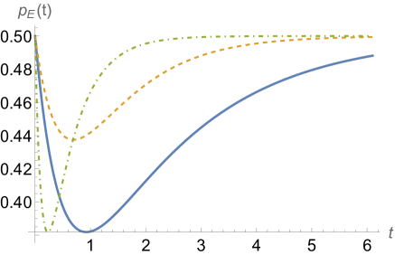
Figure 1: Minimum error probability for discriminating at time $t$ a dephasing process ${\bm{\gamma}}^{(1)}=(0,0,1)$ from those with ${\bm{\gamma}}^{(2)}=(0,0,\gamma^{(2)})$, where $\gamma^{(2)}=0.25$, $0.5$, and $4.0$ (solid, dashed, and dot-dashed lines, respectively). Entanglement provides no advantage at any time.

Two dephasing processes along orthogonal directions. Now, consider two dephasing processes aligned along orthogonal directions, e.g., corresponding to the mutually unbiased bases of $\sigma_{z}$ and $\sigma_{x}$. This means solving the case with $\bm{\gamma}^{(1)}=\{0,0,\gamma^{(1)}\}$ and $\bm{\gamma}^{(2)}=\{\gamma^{(2)},0,0\}$. As before, the dynamics corresponds to dephasing channels, but now the second channel dephases along $\sigma_{x}$, namely

$$p_{0}^{(2)}(t)=(1+e^{-2\gamma^{(2)}t})/2$$ (18)

$$p_{1}^{(2)}(t)=(1-e^{-2\gamma^{(2)}t})/2$$ (19)

$$p_{2}^{(2)}(t)=p_{3}^{(2)}(t)=0\;.$$ (20)

Thus, we obtain

$$p_{E}(t)=\tilde{p}_{E}(t)=\frac{1}{4}\left(1+e^{-2\max\{\gamma^{(1)},\gamma^{(2)}\}t}\right)\;.$$ (21)

Again, entanglement does not enhance discrimination at any time. Clearly, the optimal discrimination occurs at $t\rightarrow+\infty$, where $p_{E}^{*}=\tilde{p}_{E}^{*}=\frac{1}{4}$.

Two coplanar decaying processes. Next, consider two processes with $\bm{\gamma}^{(i)}=\{\gamma^{(i)},\gamma^{(i)},0\}$. Each process provides a set of Pauli channels with the time-dependent probabilities

$$p_{0}^{(i)}(t)=e^{-2\gamma^{(i)}t}\cosh^{2}(\gamma^{(i)}t)$$ (22)

$$p_{1}^{(i)}(t)=p_{2}^{(i)}(t)=(1-e^{-4\gamma^{(i)}t})/4$$ (23)

$$p_{3}^{(i)}(t)=e^{-2\gamma^{(i)}t}\sinh^{2}(\gamma^{(i)}t)\;.$$ (24)

In this case, entanglement improves discrimination at any time. Specifically, we have

$$\tilde{p}_{E}(t)=\frac{1}{2}-$$ (25)

$$\frac{1}{4}\max\{|e^{-2\gamma^{(1)}t}-e^{-2\gamma^{(2)}t}|,|e^{-4\gamma^{(1)}t}-e^{-4\gamma^{(2)}t}|\}\;,$$

while

$$p_{E}(t)=\frac{1}{2}-\frac{1}{4}|e^{-2\gamma^{(1)}t}-e^{-2\gamma^{(2)}t}|$$

$$-\frac{1}{8}|e^{-4\gamma^{(1)}t}-e^{-4\gamma^{(2)}t}|\;,$$ (26)

and, clearly, $p_{E}(t)<\tilde{p}_{E}(t)$. In the absence of side entanglement, since $\tilde{p}_{E}(t)$ has two absolute minima, there are two optimal times given by $t^{*}=\frac{\kappa}{\gamma^{(1)}-\gamma^{(2)}}\ln\frac{\gamma^{(1)}}{\gamma^{(2)}}$, with $\kappa=1/2$ or $1/4$. At both times, we have

$$\tilde{p}_{E}^{*}=\frac{1}{2}-\frac{1}{4}\left(\frac{\gamma^{(1)}}{\gamma^{(2)}}\right)^{\frac{\gamma^{(1)}}{\gamma^{(2)}-\gamma^{(1)}}}\left|\frac{\gamma^{(1)}}{\gamma^{(2)}}-1\right|\,.$$ (27)

On the other hand, when using entanglement, there is a unique optimal time $t^{*}$ such that $\partial_{t}p_{E}(t)=0$, which corresponds to the solution of the transcendental equation

$$\gamma^{(1)}(e^{-4\gamma^{(1)}t}+e^{-2\gamma^{(1)}t})=\gamma^{(2)}(e^{-4\gamma^{(2)}t}+e^{-2\gamma^{(2)}t})\;.$$ (28)

Figure 2 shows the error probabilities from Eqs. (25) and (26) for $\gamma^{(1)}=1$ and $\gamma^{(2)}=0.2$. The ultimate minimum error probability, $p_{E}^{*}\simeq 0.308$, is achieved using entanglement, with discrimination performed at the optimal time $t^{*}\simeq 0.782$.

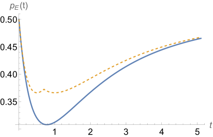
Figure 2: Minimum error probabilities for discriminating between two coplanar decaying processes with ${\bm{\gamma}}^{(1)}=(1,1,0)$ and ${\bm{\gamma}}^{(2)}=(.2,.2,0)$ at time $t$, with and without entanglement (solid and dashed lines, respectively). Side entanglement strictly improves discrimination at any time.

Two depolarising processes. In a depolarising process, the decay rates have equal and constant components. Thus, we consider the case with $\bm{\gamma}^{(i)}=\{\gamma^{(i)},\gamma^{(i)},\gamma^{(i)}\}$. The dynamics of each process gives a set depolarising channels with the time-dependent probabilities

$$p_{0}^{(i)}(t)=(1+3e^{-4\gamma^{(i)}t})/4$$ (29)

$$p_{1}^{(i)}(t)=p_{2}^{(i)}(t)=p_{3}^{(i)}(t)=(1-e^{-4\gamma^{(i)}t})/4\;.$$ (30)

Thus, we obtain

$$\tilde{p}_{E}(t)=\frac{1}{2}-\frac{1}{4}|e^{-4\gamma^{(1)}t}-e^{-4\gamma^{(2)}t}|\;,$$ (31)

$$p_{E}(t)=\frac{1}{2}-\frac{3}{8}|e^{-4\gamma^{(1)}t}-e^{-4\gamma^{(2)}t}|\;.$$ (32)

Clearly, entanglement enhances discrimination at any time. Figure 3 illustrates this for the specific values $\gamma^{(1)}=1$ and $\gamma^{(2)}=0.2$.

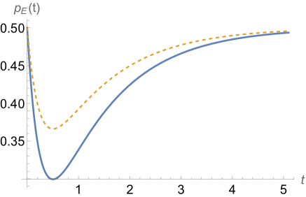
Figure 3: Minimum error probability for discriminating two depolarising processes at time $t$, with ${\bm{\gamma}}^{(1)}=(1,1,1)$ and ${\bm{\gamma}}^{(2)}=(0.2,0.2,0.2)$, with and without entanglement assistance (solid and dashed lines, respectively).

Notice that both $\tilde{p}_{E}(t)$ and $p_{E}(t)$ reach their minimum at the same optimal time

$$t^{*}=\frac{1}{4(\gamma^{(1)}-\gamma^{(2)})}\ln\frac{\gamma^{(1)}}{\gamma^{(2)}}\,,$$ (33)

with the corresponding ultimate minimum error probabilities given by

$$\tilde{p}_{E}^{*}=\frac{1}{2}-\frac{1}{4}\left(\frac{\gamma^{(1)}}{\gamma^{(2)}}\right)^{\frac{\gamma^{(1)}}{\gamma^{(2)}-\gamma^{(1)}}}\left|\frac{\gamma^{(1)}}{\gamma^{(2)}}-1\right|\,,$$ (34)

$$p_{E}^{*}=\frac{1}{2}-\frac{3}{8}\left(\frac{\gamma^{(1)}}{\gamma^{(2)}}\right)^{\frac{\gamma^{(1)}}{\gamma^{(2)}-\gamma^{(1)}}}\left|\frac{\gamma^{(1)}}{\gamma^{(2)}}-1\right|\,.$$ (35)

These error probabilities are shown in Fig. 4 as a function of the ratio of the decay parameters $\gamma^{(1)}$ and $\gamma^{(2)}$.

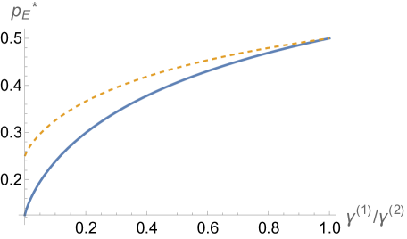
Figure 4: Ultimate minimum error probabilities in discriminating between two depolarising processes as a function of the ratio the decay rates, with and without entanglement assistance (solid and dashed lines, respectively). In both cases, the optimal discrimination time is given in Eq. (33).

A depolarising and a dephasing process. Finally, let us consider the problem of distinguishing between a depolarising process, $\bm{\gamma}^{(1)}=\{\gamma^{(1)},\gamma^{(1)},\gamma^{(1)}\}$, and a dephasing process, $\bm{\gamma}^{(2)}=\{0,0,\gamma^{(2)}\}$. For a strategy with no use of entanglement the error probability is given by

$$\tilde{p}_{E}(t)=\frac{1}{2}-$$ (36)

$$\frac{1}{4}\max\{1-e^{-4\gamma^{(1)}t},|e^{-4\gamma^{(1)}t}-e^{-2\gamma^{(2)}t}|\}\;.$$

In this case, the infimum is achieved in the limit $t\rightarrow+\infty$, where $\tilde{p}_{E}^{*}=\frac{1}{4}$.

By utilizing entanglement, the error probability is instead given by

$$p_{E}(t)=\frac{1}{2}-\frac{1}{8}(1-e^{-4\gamma^{(1)}t})$$

$$-\frac{1}{16}|1-3e^{-4\gamma^{(1)}t}+2e^{-2\gamma^{(2)}t}|$$

$$-\frac{1}{16}|1+e^{-4\gamma^{(1)}t}-2e^{-2\gamma^{(2)}t}|\;.$$ (37)

The comparison between these two strategies is more intricate than in previous cases. By analyzing the two functions (36) and (37), we find that they are equal $p_{E}(t)=\tilde{p}_{E}(t)=\frac{1}{4}(1+e^{-4\gamma^{(1)}}t)$ at all times when

$$3e^{-4\gamma^{(1)}t}-1\leq 2e^{-2\gamma^{(2)}t}\leq e^{-4\gamma^{(1)}t}+1\;.$$ (38)

To determine whether entanglement provides a strict advantage, we must identify a time $t^{*}$ at which $p_{E}(t)$ reaches a minimum value lower than $\frac{1}{4}$. Notice that the condition $p_{E}(t)\leq\frac{1}{4}$ can be satisfied in the region

$$e^{-2\gamma^{(2)}t}\geq(3e^{-4\gamma^{(1)}t}+1)/2\;,$$ (39)

where

$$p_{E}(t)=(3+3e^{-4\gamma^{(1)}t}-2e^{-2\gamma^{(2)}t})/8\;.$$ (40)

In fact, numerical inspection shows that this condition holds as long as $\frac{\gamma^{(2)}}{\gamma^{(1)}}\lesssim 0.3785$. In this case the minimum of $p_{E}(t)$ in Eq. (40) is reached at $t^{*}=\frac{1}{4\gamma^{(1)}-2\gamma^{(2)}}\ln\frac{3\gamma^{(1)}}{\gamma^{(2)}}$, with a corresponding minimum error probability

$$p^{*}_{E}\!=\!\frac{3}{8}\left[1-\left(\frac{3\gamma^{(1)}}{\gamma^{(2)}}\right)^{\frac{2\gamma^{(1)}}{\gamma^{(2)}-2\gamma^{(1)}}}\left(\frac{2\gamma^{(1)}}{\gamma^{(2)}}-1\right)\right]<\frac{1}{4}\,.$$ (41)

Thus, when $\frac{\gamma^{(2)}}{\gamma^{(1)}}\lesssim 0.3785$, entanglement provides a strict advantage in discrimination at a finite time. Figure 5 illustrates this threshold, where the benefits of entanglement are clearly visible.

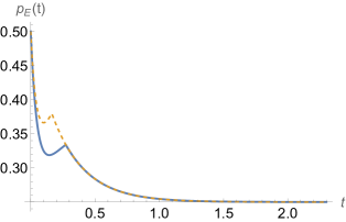
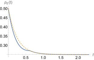
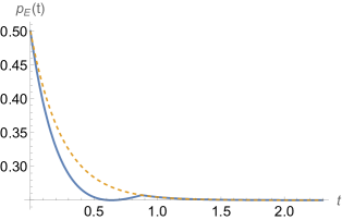
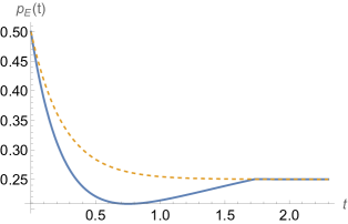
Figure 5: Minimum error probability for discriminating the depolarising process ${\bm{\gamma}}^{(1)}=(1,1,1)$ from a dephasing process ${\bm{\gamma}}^{(2)}=(0,0,\gamma^{(2)})$ with and without side entanglement (solid and dashed lines, respectively), for different values of $\gamma^{(2)}$: $10$ (top left), $0.5$ (top right), $0.3785$ (bottom left), and $0.2$ (bottom right).

In conclusion, the results presented in this paper deepen our understanding of quantum dynamical processes and their discrimination, offering new insights into the interplay between entanglement, timing, and optimal measurement strategies. By elucidating the benefits of entanglement and proper timing, this study lays the foundation for designing more efficient protocols and highlights the potential for further exploration of quantum correlations in dynamical settings. Finally, it is worth noting that in quantum illumination protocols, the optimal timing can be typically related to the optimal distance from the target under test.

This work has been sponsored by PRIN MUR Project 2022SW3RPY.

References

- (1) C. W. Helstrom, Quantum Detection and Estimation Theory (Academic Press, New York, 1976).
- (2) I. D. Ivanovic, Phys. Lett. A 123, 257 (1987); D. Dieks, ibid. 126, 303 (1988); A. Peres, ibid. 128, 19 (1988); G. Jaeger and A. Shimony, ibid. 197, 83 (1995).
- (3) J. Walgate, A. J. Short, L. Hardy, and V. Vedral, Phys. Rev. Lett. 85, 4972 (2000); S. Virmani, M. F. Sacchi, M. B. Plenio, and D. Markham, Phys. Lett. A 288, 62 (2001).
- (4) J. Bergou, U. Herzog, and M. Hillery, Quantum state estimation, Lecture Notes in Physics Vol. 649 (Springer, Berlin, 2004), p. 417; A. Chefles, ibid., p. 467.
- (5) G. M. D’Ariano, M. F. Sacchi, and J. Kahn, Phys. Rev. A 72, 032310 (2005); F. Buscemi and M. F. Sacchi, Phys. Rev. A 74, 052320 (2006); J. Bae and L.-C. Kwek, J. Phys. A 48, 083001 (2015).
- (6) A. M. Childs, J. Preskill, and J. Renes, J. Mod. Opt. 47, 155 (2000); A. Acín, Phys. Rev. Lett. 87, 177901 (2001); G. M. D’Ariano, P. Lo Presti, and M. G. A. Paris, Phys. Rev. Lett. 87, 270404 (2001).
- (7) M. F. Sacchi, Phys. Rev. A 71, 062340 (2005).
- (8) M. F. Sacchi, Phys. Rev. A 72, 014305 (2005).
- (9) G. Chiribella, G. M. D’Ariano, and P. Perinotti, Phys. Rev. Lett. 101, 180501 (2008); K. Nakahira and K. Kato, Phys. Rev. Lett. 126, 200502 (2021); S. K. Oskouei, S. Mancini, and M. Rexiti, Proc. R. Soc. A 479, 20220796 (2023).
- (10) S. Lloyd, Science 321, 1463 (2008); S.-H. Tan, B. I. Erkmen, V. Giovannetti, S. Guha, S. Lloyd, L. Maccone, S. Pirandola, and J. H. Shapiro, Phys. Rev. Lett. 101, 253601 (2008); M. Sanz, U. Las Heras, J. J. García-Ripoll, E. Solano, and R. Di Candia, Phys. Rev. Lett. 118, 070803 (2017); J. H. Shapiro, IEEE Aerospace and Electronic Systems Magazine 35, 8 (2020).
- (11) M. F. Sacchi, J. Opt. B 7, S333 (2005).
- (12) G. M. D’Ariano, M. F. Sacchi, and J. Kahn, Phys. Rev. A 72, 052302 (2005).
- (13) H.-P. Breuer and F. Petruccione, The theory of open quantum systems (Oxford University Press, Oxford, 2002); A. Rivas and S. F. Huelga, Open quantum systems, Vol. 10 (Springer, Berlin/Heidelberg, 2012).
- (14) V. I. Paulsen, Completely Bounded Maps and Dilations (Longman Scientific and Technical, New York, 1986).
- (15) D. Aharonov, A. Kitaev, and N. Nisan, in “Proceedings of the 30th Annual ACM Symposium on Theory of Computation (STOC)”, p. 20, 1997.
- (16) D. Chruściński and F. A. Wudarski, Phys. Lett. A 377, 1425 (2013).