Spatiotemporal Synchronization of Distributed Arrays using Particle-Based Loopy Belief Propagation

Abstract

Sensing and imaging with distributed radio infrastructures (e.g., distributed MIMO, wireless sensor networks, multistatic radar) rely on knowledge of the positions, orientations, and clock parameters of distributed apertures. We extend a particle-based loopy belief propagation (BP) algorithm to cooperatively synchronize distributed agents to anchors in space and time. Substituting marginalization over nuisance parameters with approximate but closed-form concentration, we derive an efficient estimator that bypasses the need for preliminary channel estimation and operates directly on noisy channel observations. Our algorithm demonstrates scalable, accurate spatiotemporal synchronization on simulated data.

Index Terms—  Cooperative positioning, synchronization

1 Introduction

Distributed antenna arrays exploit spatially separated nodes to achieve higher aperture gain, interference immunity, and improved spatial diversity for sensing or communications. However, such arrays require precise synchronization of time, phase, and frequency to ensure coherent summation of the signal carrier at the location of a target [1, 2]. This is especially challenging at millimeter-wave frequencies and GHz‐wide modulation bandwidths, where clocks at different nodes must remain aligned despite drift. Optical links can synchronize spatially separated clocks at femtosecond precision [3] but are difficult to implement in dynamic scenarios due to strict pointing/tracking requirements and large form factors. Therefore, over-the-air (OTA) wireless time synchronization techniques at microwave and millimeter-wave frequencies are of great interest [4, 1].

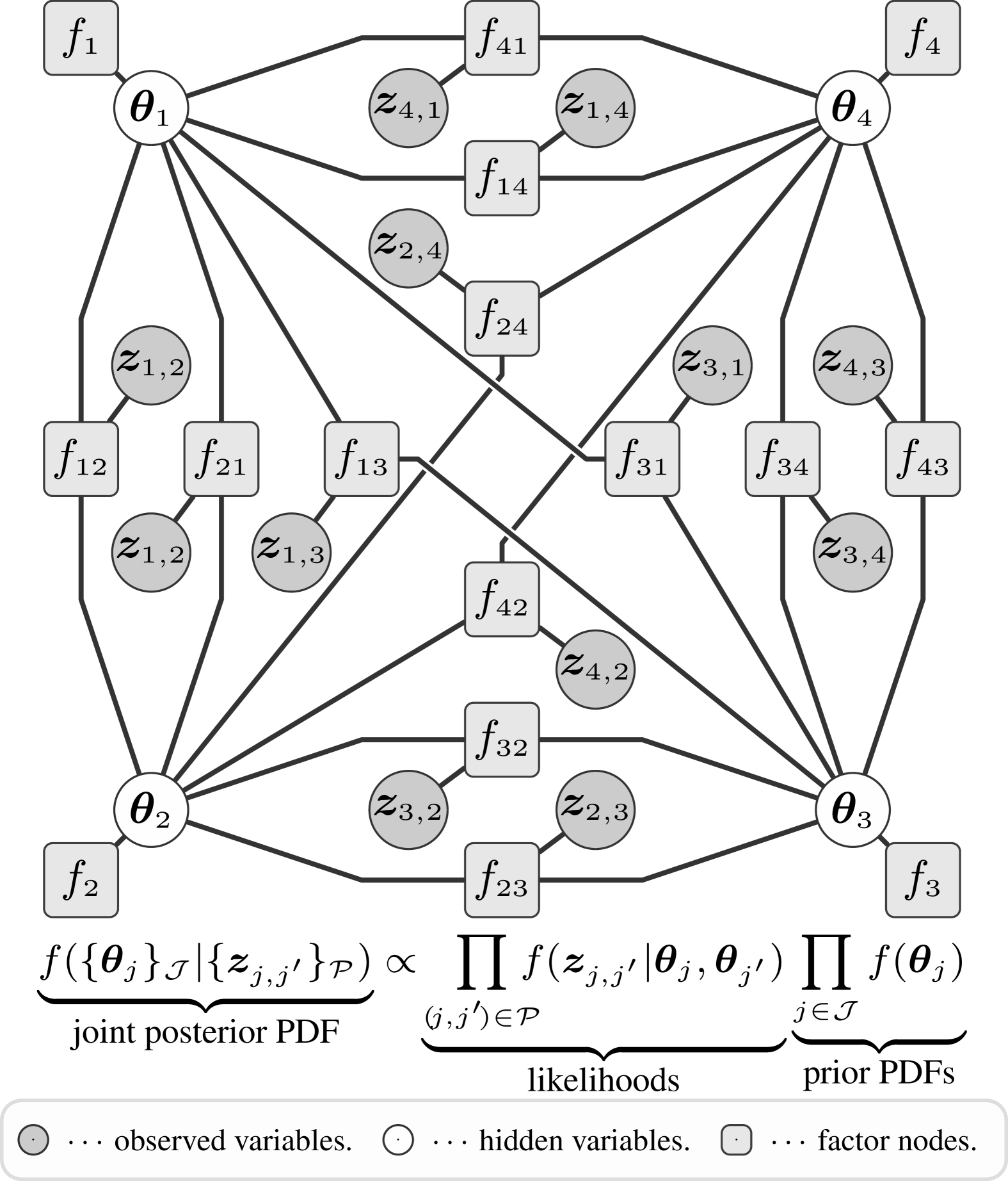
Fig. 1: Factor graph representing the joint posterior PDF.
We abbreviate $f_{\scriptscriptstyle jj^{\prime}}:=f\big{(}\bm{z}_{\scriptscriptstyle j,j^{\prime}}|\bm{\theta}_{\scriptscriptstyle j},\bm{\theta}_{\scriptscriptstyle j^{\prime}}\big{)}$ and $f_{\scriptscriptstyle j}:=f\big{(}\bm{\theta}_{\scriptscriptstyle j}\big{)}$.

Prominent approaches are consensus-based time synchronization techniques [5] because they scale with the size of the network and are robust to node failures. However, the accuracy of time synchronization is affected by message delays. The message delays include propagation time and the transmission, media access, and reception process [6]. In a dynamic scenario with moving platforms the random message delays may be orders of magnitude larger than the required precision and can cause synchronization algorithms to diverge.

Contributions. We build upon the efficient particle-based loopy belief propagation (BP) algorithm from [7], [8, Sec. 2.4] where we extend the problem of finding the positions and clock parameters of distributed apertures to three-dimensional (3D) spatiotemporal synchronization, i.e., joint inference of the spatial states (positions and orientations) and the temporal states (clock parameters) of the distributed apertures. While the original algorithm works in a two-step fashion (using intermediate channel parameter estimates such as delays), our algorithm works directly on the noisy channel estimates between distributed apertures and does not require a dedicated channel estimator. We leverage concentration to eliminate nuisance parameters as an approximate but closed-form solution that avoids computationally involved marginalizations.

2 System Model

We consider a set $\mathcal{J}:=\{1\dots J\}=\mathcal{M}\cup\mathcal{A}$ of geometrically identical apertures comprising a set of agents $\mathcal{M}$ with unknown spatiotemporal parameters and a set of anchors $\mathcal{A}$ with known spatiotemporal parameters

$$\bm{\theta}_{\scriptscriptstyle j}:=\left[{\bm{p}_{\scriptscriptstyle j}}^{\mathsf{T}}\ {\bm{\eta}^{\text{\tiny{o}}}_{\scriptscriptstyle j}}^{\mathsf{T}}\epsilon_{j}\right]^{\mathsf{T}}\quad\in\mathcal{S}_{\scriptscriptstyle\!\bm{\theta}}$$ (1)

in global coordinates where the state space $\mathcal{S}_{\scriptscriptstyle\!\bm{\theta}}\!=\!\mathbb{R}^{7}$ comprises the position $\bm{p}_{\scriptscriptstyle j}\!=\!\mathbb{R}^{3}$, orientation $\bm{\eta}^{\text{\tiny{o}}}_{\scriptscriptstyle j}\!=\!\mathbb{R}^{3}$ and clock time offset $\epsilon_{j}$. We assume that each aperture $j^{\prime}\!\in\!\mathcal{J}$ transmits a pilot which the receiving apertures $j\!\in\!\mathcal{J}\!\setminus\!j^{\prime}$ use to compute noisy channel observations

$$\bm{z}_{\scriptscriptstyle j,j^{\prime}}:=\alpha_{\scriptscriptstyle\!j,j^{\prime}}\,\bm{\psi}_{\scriptscriptstyle j,j^{\prime}}(\bm{\theta}_{\scriptscriptstyle j},\bm{\theta}_{\scriptscriptstyle j^{\prime}})+\bm{w}_{\scriptscriptstyle j,j^{\prime}}\quad\in\mathbb{C}^{N}$$ (2)

taken in spatially and temporally uncorrelated noise $\bm{w}_{\scriptscriptstyle j,j^{\prime}}\!\sim\!\mathcal{CN}(\bm{0},\sigma^{2}_{\scriptscriptstyle j,j^{\prime}}\mathbf{I}_{\scriptscriptstyle N})$ with amplitudes $\alpha_{\scriptscriptstyle\!j,j^{\prime}}\in\mathbb{C}^{N}$. Let $\mathbb{S}^{1}\!=\!\{x\!\in\!\mathbb{C}\!:\!|x|\!=\!1\}$ denote the $1$-sphere, i.e., the unit-circle, and let $\mathbb{T}^{N}\!\equiv\!(\mathbb{S}^{1})^{N}$ denote the $N$-torus, one particular steering vector $\bm{\psi}_{\scriptscriptstyle j,j^{\prime}}(\bm{\theta}_{\scriptscriptstyle j},\bm{\theta}_{\scriptscriptstyle j^{\prime}})\!\in\!\mathbb{T}^{N}$ is from the spatiotemporal array manifold

$$\bm{\psi}=\bm{b}(\tau)\otimes\bm{a}(\theta^{\text{\tiny AoA}}\!,\!\vartheta^{\text{\tiny AoA}})\otimes\bm{a}(\theta^{\text{\tiny AoD}}{}{}\!,\!\vartheta^{\text{\tiny AoD}}{}{})$$ (3)

modeled as the Kronecker product of the temporal manifold

$$\bm{b}(\tau)=\exp\big{(}\!-\!\mathrm{j}2\pi\bm{f}\tau\big{)}\quad\in\mathbb{T}^{N_{\scriptscriptstyle\!f}}$$ (4)

with the spatial manifolds in angle of arrival (AoA) and angle of departure (AoD) [9] $\bm{a}(\theta,\vartheta)=\bm{a}_{y}(\theta,\vartheta)\otimes\bm{a}_{z}(\theta)$ each being itself a Kronecker product of the “horizontal” manifold

$$\bm{a}_{y}(\theta,\vartheta)=\exp\Big{(}\mathrm{j}\frac{2\pi}{\lambda}\bm{p}_{y}\sin(\theta)\sin(\vartheta)\Big{)}\quad\in\mathbb{T}^{M_{y}}$$ (5)

and “vertical” manifold

$$\bm{a}_{z}(\theta)=\exp\Big{(}\mathrm{j}\frac{2\pi}{\lambda}\bm{p}_{z}\cos(\theta)\Big{)}\quad\in\mathbb{T}^{M_{z}}\,$$ (6)

for wavelength $\lambda$. We use $\bm{f}\in\mathbb{R}^{N_{\scriptscriptstyle\!f}}$ to denote a vector of $N_{\scriptscriptstyle\!f}$ baseband frequencies, $\bm{p}_{y}\in\mathbb{R}^{M_{y}}$ a vector of $M_{y}$ horizontal sensor positions and $\bm{p}_{z}\in\mathbb{R}^{M_{z}}$ a vector of $M_{z}$ vertical sensor positions of a “template” aperture. The complete manifold in (3) is of dimension $N\triangleq N_{\scriptscriptstyle\!f}M_{y}^{2}M_{z}^{2}$. We require each of the support vectors $\{\bm{f},\bm{p}_{y},\bm{p}_{z}\}$ to be symmetric around $0$. The steering vectors are elements of the manifolds parameterized by local parameters in spherical aperture coordinates with

$$\widetilde{\tau}_{\scriptscriptstyle j,j^{\prime}}=\frac{\lVert\acute{\bm{r}}_{\scriptscriptstyle j,j^{\prime}}\rVert}{\mathsf{c}}+(\epsilon_{j}-\epsilon_{j^{\prime}})$$ (7)

denoting the perceived delay and $\mathsf{c}$ the propagation velocity,

$$\theta(\bm{r})=\arccos(r_{\scriptscriptstyle z}/\lVert\bm{r}\rVert)$$ (8)

denoting elevation, and

$$\vartheta(\bm{r})=\operatorname{arctan2}(r_{\scriptscriptstyle y},r_{\scriptscriptstyle x})$$ (9)

denoting azimuth, for one arbitrary vector $\bm{r}=[r_{x},r_{y},r_{z}]^{\mathsf{T}}$ in Cartesian aperture coordinates.

Mapping from global to local parameters. Let $\bm{r}_{\scriptscriptstyle j,j^{\prime}}\!:=\!\bm{p}_{\scriptscriptstyle j^{\prime}}\!-\!\bm{p}_{\scriptscriptstyle j}$ be the vector pointing from the phase center of aperture $j$ to aperture $j^{\prime}$ in global coordinates, we define the AoA as $\{\theta_{\scriptscriptstyle j,j^{\prime}}^{\text{\tiny AoA}},\vartheta_{\scriptscriptstyle j,j^{\prime}}^{\text{\tiny AoA}}\}\!:=\!\{\theta(\acute{\bm{r}}_{\scriptscriptstyle j,j^{\prime}}),\vartheta(\acute{\bm{r}}_{\scriptscriptstyle j,j^{\prime}})\}$ parameterized by the vector $\acute{\bm{r}}_{\scriptscriptstyle j,j^{\prime}}\!=\!\bm{M}_{\scriptscriptstyle j}^{-1}\bm{r}_{\scriptscriptstyle j,j^{\prime}}$ pointing from receiving aperture $j$ to transmitting aperture $j^{\prime}$ in local Cartesian coordinates of aperture $j$. Likewise, we define the AoD as $\{\theta_{\scriptscriptstyle j,j^{\prime}}^{\text{\tiny AoD}},\vartheta_{\scriptscriptstyle j,j^{\prime}}^{\text{\tiny AoD}}\}\!:\!=\{\theta(\grave{\bm{r}}_{\scriptscriptstyle j,j^{\prime}}),\vartheta(\grave{\bm{r}}_{\scriptscriptstyle j,j^{\prime}})\}$ parameterized by the vector $\grave{\bm{r}}_{\scriptscriptstyle j,j^{\prime}}\!=\!\bm{M}_{\scriptscriptstyle j^{\prime}}^{-1}(-\bm{r}_{\scriptscriptstyle j,j^{\prime}})$ pointing from transmitting aperture $j^{\prime}$ to receiving aperture $j$ in local Cartesian coordinates of aperture $j^{\prime}$. Let $\bm{1}_{\scriptscriptstyle{M\times N}}$ denote an $(M\times N)$-matrix of all ones, we model the uniform rectangular array (URA) sensor layout

$$\bm{P}_{\text{t}}:=\left[\begin{array}[]{*{20}{C}}\>\lx@intercol\hfil\bm{0}\hfil\>\>\\ \>\lx@intercol\hfil\bm{p}_{y}^{\mathsf{T}}\otimes\bm{1}_{\scriptscriptstyle{1\times M_{z}}}\hfil\>\>\\ \>\lx@intercol\hfil\bm{1}_{\scriptscriptstyle{1\times M_{y}}}\otimes\bm{p}_{z}^{\mathsf{T}}\hfil\>\>\\ \end{array}\right]\quad\in\mathbb{R}^{3\times M_{y}M_{z}}$$ (13)

of the template aperture in the $yz$-plane, symmetric about the origin $\bm{0}$. The antenna positions of an actual physical aperture are computed by shifting a “template” aperture out of the origin $\bm{0}$ to its center position ${\bm{p}_{\text{\tiny c}\scriptscriptstyle,j}^{\scriptscriptstyle(\!0,0\!)}}$ in global coordinates through [10]

$$\bm{P}_{\scriptscriptstyle j}^{(\!0,0\!)}={\bm{p}_{\text{\tiny c}\scriptscriptstyle,j}^{\scriptscriptstyle(\!0,0\!)}}\,\bm{1}_{\scriptscriptstyle{1\times M}}\,+\bm{M}_{\scriptscriptstyle j}\bm{P}_{\text{t}}\quad\in\mathbb{R}^{3\times M}.$$ (14)

The matrix $\bm{M}_{\scriptscriptstyle j}\in SO(3)$ is a rotation matrix that defines the orientation of aperture $j$ in global coordinates. It is from the special orthogonal group $SO(3)\!=\!\{\bm{M}\!\in\!\mathbb{R}^{3\times 3}|\bm{M}\bm{M}^{\mathsf{T}}=\bm{M}^{\mathsf{T}}\bm{M}\!=\!\mathbf{I}_{\scriptscriptstyle 3},\det(\bm{M})\!=\!1\}$. In this work, we use a parameterization $\bm{M}_{\scriptscriptstyle j}(\bm{\eta}^{\text{\tiny{o}}}_{\scriptscriptstyle j})$ with $\bm{\eta}^{\text{\tiny{o}}}_{\scriptscriptstyle j}\!\in\!\mathbb{R}^{3\times 1}$ in Euler angles [11, p. 86], although a parameterization in unit quaternions [11, p. 168] is likewise possible. In the scenario (see Fig. 2), all aperture orientations are chosen outside of the gimbal lock (e.g., the pitch angle $\theta^{\text{\tiny r}}_{\scriptscriptstyle j}\neq\pm\nicefrac{{\pi}}{{2}}$).

Fig. 2: Scenario: Anchors $\mathcal{A}\!=\!\{1,4\}$ and agents $\mathcal{M}\!=\!\{2,3\}$.

3 Statistical Model

Deterministic Concentrated Likelihood. We use a deterministic concentrated likelihood model assuming that the amplitudes $\alpha_{\scriptscriptstyle\!j,j^{\prime}}$ are deterministic unknowns [12]. Per (2), the aperture-to-aperture channel observation is distributed as $\bm{z}_{\scriptscriptstyle j,j^{\prime}}|\bm{\theta}_{\scriptscriptstyle j},\bm{\theta}_{\scriptscriptstyle j^{\prime}}=\mathcal{CN}(\alpha_{\scriptscriptstyle\!j,j^{\prime}}\bm{\psi}_{\scriptscriptstyle j,j^{\prime}},\sigma^{2}_{\scriptscriptstyle j,j^{\prime}}\mathbf{I}_{\scriptscriptstyle N})$. Assuming independent observations between all $|\mathcal{P}|\!=\!\frac{J!}{(J-2)!}\!=\!J(J\!-\!1)$ ordered aperture pairs $(\!j,j^{\prime}\!)\!\in\!\mathcal{P}\!=\!\big{\{}(\!j,j^{\prime}\!)\!\in\!\mathcal{J}^{2}\!:\!j\!\neq\!j^{\prime}\big{\}}$, the joint likelihood factorizes as

$$\begin{split}&f\big{(}\{\bm{z}_{\scriptscriptstyle j,j^{\prime}}\}_{\scriptscriptstyle\mathcal{P}}|\{\bm{\theta}_{\scriptscriptstyle j}\}_{\scriptscriptstyle\mathcal{J}},\{\alpha_{\scriptscriptstyle\!j,j^{\prime}},\sigma^{2}_{\scriptscriptstyle j,j^{\prime}}\}_{\scriptscriptstyle\mathcal{P}}\big{)}\\ &=\!\!\prod_{(\!j,j^{\prime}\!)\in\mathcal{P}}\!\frac{\exp\left(-\frac{1}{\sigma^{2}_{\scriptscriptstyle j,j^{\prime}}}\big{\|}\bm{z}_{\scriptscriptstyle j,j^{\prime}}-\bm{\psi}_{\scriptscriptstyle j,j^{\prime}}(\bm{\theta}_{\scriptscriptstyle j},\bm{\theta}_{\scriptscriptstyle j^{\prime}})\alpha_{\scriptscriptstyle\!j,j^{\prime}}\big{\|}^{2}\right)}{\left(\pi\sigma^{2}_{\scriptscriptstyle j,j^{\prime}}\right)^{N}}\,.\end{split}$$ (15)

We compute the profile likelihood by concentrating w.r.t. the nuisance parameters $\{\alpha_{\scriptscriptstyle\!j,j^{\prime}},\sigma^{2}_{\scriptscriptstyle j,j^{\prime}}\}_{\scriptscriptstyle\mathcal{P}}$. That is, we compute maximum likelihood (ML) estimates conditional on the state pairs $\{\bm{\theta}_{\scriptscriptstyle j},\bm{\theta}_{\scriptscriptstyle j^{\prime}}\}$ as [13, 14, 10]

$$\widehat{\alpha}_{\scriptscriptstyle\!j,j^{\prime}}|\bm{\theta}_{\scriptscriptstyle j},\!\bm{\theta}_{\scriptscriptstyle j^{\prime}} =\frac{1}{N}~\bm{\psi}_{\scriptscriptstyle j,j^{\prime}}^{\mathsf{H}}\,\bm{z}_{\scriptscriptstyle j,j^{\prime}}~,$$ (16)

$$\widehat{\sigma^{2}}_{\scriptscriptstyle j,j^{\prime}}|\bm{\theta}_{\scriptscriptstyle j},\!\bm{\theta}_{\scriptscriptstyle j^{\prime}} =\frac{1}{N}~\operatorname{tr}\Big{(}\bm{\Pi}_{\scriptscriptstyle{j},{j^{\prime}}}^{\perp}\widehat{\bm{R}}_{\scriptscriptstyle j,j^{\prime}}^{\text{\scriptsize e}}\Big{)}~,$$ (17)

where $\bm{\Pi}_{\scriptscriptstyle{j},{j^{\prime}}}^{\perp}(\bm{\theta}_{\scriptscriptstyle j},\!\bm{\theta}_{\scriptscriptstyle j^{\prime}}\!)\!=\!\mathbf{I}_{\scriptscriptstyle N}\!-\!\frac{\bm{\psi}_{\scriptscriptstyle j,j^{\prime}}\bm{\psi}_{\scriptscriptstyle j,j^{\prime}}^{\mathsf{H}}}{N}$ is the projector onto the noise subspace, and the sample covariance matrix $\widehat{\bm{R}}_{\scriptscriptstyle j,j^{\prime}}^{\text{\scriptsize e}}\!:=\!\bm{z}_{\scriptscriptstyle j,j^{\prime}}\,\bm{z}_{\scriptscriptstyle j,j^{\prime}}^{\mathsf{H}}$ is an empirical rank-$1$ estimate of the spatiotemporal observation covariance matrix $\bm{R}_{\scriptscriptstyle j,j^{\prime}}=\mathbb{E}\big{(}\bm{z}_{\scriptscriptstyle j,j^{\prime}}\bm{z}_{\scriptscriptstyle j,j^{\prime}}^{\mathsf{H}}\big{)}$. Although notationally brief, (17) can be implemented efficiently using (24) in Appendix A. Reinsertion of $\widehat{\alpha}_{\scriptscriptstyle\!j,j^{\prime}}|\bm{\theta}_{\scriptscriptstyle j},\!\bm{\theta}_{\scriptscriptstyle j^{\prime}}$ and $\widehat{\sigma^{2}}_{\scriptscriptstyle j,j^{\prime}}|\bm{\theta}_{\scriptscriptstyle j},\!\bm{\theta}_{\scriptscriptstyle j^{\prime}}$ in (LABEL:eq:lhf-det) yields the deterministic profile likelihood function for a single observation

$$\begin{split}&f\big{(}\bm{z}_{\scriptscriptstyle j,j^{\prime}}|\bm{\theta}_{\scriptscriptstyle j},\bm{\theta}_{\scriptscriptstyle j^{\prime}}\big{)}=\frac{\exp\Big{(}-\frac{1}{\widehat{\sigma^{2}}_{\scriptscriptstyle j,j^{\prime}}}\big{\|}\bm{\Pi}_{\scriptscriptstyle{j},{j^{\prime}}}^{\perp}\bm{z}_{\scriptscriptstyle j,j^{\prime}}\big{\|}^{2}\Big{)}}{\big{(}\pi\widehat{\sigma^{2}}_{\scriptscriptstyle j,j^{\prime}}\big{)}^{N}}\,.\end{split}$$ (18)

Factor Graph. The joint posterior probability density function (PDF) (up to a proportionality constant) of all aperture states conditional on all observations is represented by the factor graph [15] in Fig. 1 (for $J\!=\!4$) which, by exploiting the conditional independence structure that the graph makes explicit, can be shown to factorize as $f(\{\bm{\theta}_{\scriptscriptstyle j}\}_{\scriptscriptstyle\mathcal{J}}|\{\bm{z}_{\scriptscriptstyle j,j^{\prime}}\}_{\scriptscriptstyle\mathcal{P}})\propto\!\prod_{\scriptscriptstyle(\!j,j^{\prime}\!)\in\mathcal{P}}\!f(\bm{z}_{\scriptscriptstyle j,j^{\prime}}|\bm{\theta}_{\scriptscriptstyle j},\bm{\theta}_{\scriptscriptstyle j^{\prime}})\prod_{\scriptscriptstyle j\in\mathcal{J}}f(\bm{\theta}_{\scriptscriptstyle j})$ into a product of the (concentrated) likelihoods in (LABEL:eq:lhf-det-concentrated) with prior PDFs $f(\bm{\theta}_{\scriptscriptstyle j})$ of the states of all apertures $j$. We aim to compute the minimum mean square error (MMSE) state estimate of aperture $j$ as the expectation under marginal posterior PDFs as

$$\hat{\bm{\theta}}^{\text{\tiny MMSE}}_{\scriptscriptstyle j}=\mathbb{E}\big{(}\bm{\theta}_{\scriptscriptstyle j}|\{\bm{z}_{\scriptscriptstyle j,j^{\prime}}\}_{\scriptscriptstyle\mathcal{P}}\big{)}\,.$$ (19)

To obtain the marginal PDFs $f(\bm{\theta}_{\scriptscriptstyle j}|\{\bm{z}_{\scriptscriptstyle j,j^{\prime}}\}_{\scriptscriptstyle\mathcal{P}})$, the sum-product algorithm (SPA) [16, Sec. 8.4.4] would result in exact inference in tree-structured factor graphs. However, problems of the class of cooperative localization result in graphs with loops where approximate inference [17, Sec. V] is possible by iteratively applying the SPA resulting in loopy BP [18].

Loopy BP. Let $\mathcal{M}_{\scriptscriptstyle j}\!:=\!\{(\grave{\iota},\acute{\iota})\in\mathcal{J}^{2}|(\grave{\iota}=j\lor\acute{\iota}=j)\land\grave{\iota}\neq\acute{\iota}\}\subset\mathcal{P}$ define the set of aperture pairs that involve aperture $j$. Further, let $\overline{\bm{z}}_{\scriptscriptstyle j}\!:=\![\bm{z}_{\scriptscriptstyle j,j^{\prime}}]_{\scriptscriptstyle(\!j,j^{\prime}\!)\in\mathcal{P}}$ and $\overline{\bm{\theta}}\!:=\![\bm{\theta}_{\scriptscriptstyle j}]_{\scriptscriptstyle j\in\mathcal{J}}$, $\widetilde{\bm{\theta}}_{\scriptscriptstyle j}\!:=\![\bm{\theta}_{\scriptscriptstyle j^{\prime}}]_{\scriptscriptstyle j^{\prime}\in\mathcal{J}\setminus j}$ denote vectors of stacked [8] observations and states, respectively. We devise iterative BP message passing [19] where in each message passing iteration $p\!\in\!\{1\dots P\}$ we compute the beliefs [8]

$$b^{\scriptscriptstyle(p)}\!(\bm{\theta}_{\scriptscriptstyle j})\! \propto\!\!\int\!\!b^{\scriptscriptstyle(p)}(\overline{\bm{\theta}})\mathrm{d}\widetilde{\bm{\theta}}_{\scriptscriptstyle j}$$ (20)

$$=\!\!f(\bm{\theta}_{\scriptscriptstyle j})\!\!\int\!\!\!\prod_{\scriptscriptstyle(\grave{\iota},\acute{\iota})\in\mathcal{P}}\!\!\!f(\bm{z}_{\scriptscriptstyle\grave{\iota},\acute{\iota}}|\bm{\theta}_{\scriptscriptstyle\grave{\iota}},\bm{\theta}_{\scriptscriptstyle\acute{\iota}})\!\prod_{\scriptscriptstyle j^{\prime}\!\in\mathcal{J}\setminus j}\!\!\!b^{\scriptscriptstyle(p\!-\!1)}\!(\bm{\theta}_{\scriptscriptstyle j^{\prime}\!})\mathrm{d}\widetilde{\bm{\theta}}_{\scriptscriptstyle j}$$

$$\propto\!\!f(\bm{\theta}_{\scriptscriptstyle j})\!\!\int\!\!\!\prod_{\scriptscriptstyle(\grave{\iota},\acute{\iota})\in\mathcal{M}_{\scriptscriptstyle j}}\!\!\!f(\bm{z}_{\scriptscriptstyle\grave{\iota},\acute{\iota}}|\bm{\theta}_{\scriptscriptstyle\grave{\iota}},\bm{\theta}_{\scriptscriptstyle\acute{\iota}})\!\prod_{\scriptscriptstyle j^{\prime}\!\in\mathcal{J}\setminus j}\!\!\!b^{\scriptscriptstyle(p\!-\!1)}\!(\bm{\theta}_{\scriptscriptstyle j^{\prime}\!})\mathrm{d}\widetilde{\bm{\theta}}_{\scriptscriptstyle j}$$

which are approximations of the marginal posterior PDFs $f(\bm{\theta}_{\scriptscriptstyle j}|\overline{\bm{z}}_{\scriptscriptstyle j})$. Note that the marginalization integral reduces the likelihood factor multiplication over the set of all aperture pairs $\mathcal{P}$ to a multiplication over the set $\mathcal{M}_{\scriptscriptstyle j}$ of likelihood factors connected to aperture $j$, thereby exploiting the conditional independence structure of the graph. According to the rules of the SPA, the marginal posterior PDF $f(\bm{\theta}_{\scriptscriptstyle j}|\overline{\bm{z}}_{\scriptscriptstyle j})$ of aperture $j$ computes as the product of all incoming messages, one of which is the prior $f(\bm{\theta}_{\scriptscriptstyle j})$ of node $j$. In a graph such as in Fig. 1, the other messages compute as the marginalization integrals of the product of the marginal posterior PDFs of all other nodes $j^{\prime}\in\mathcal{J}\setminus j$ with the likelihood factors connecting them to node $j$ (i.e., $\prod_{(\grave{\iota},\acute{\iota})\in\mathcal{M}_{\scriptscriptstyle j}}f_{\scriptscriptstyle\grave{\iota}\acute{\iota}}$). Since the graph has loops, the marginal posterior PDFs, approximated by the beliefs $b^{\scriptscriptstyle(p)}\!(\bm{\theta}_{\scriptscriptstyle j})$, of all nodes $\bm{\theta}_{\scriptscriptstyle j}$ depend on the marginal posterior PDFs of all other nodes and are hence updated iteratively using loopy BP.

4 Particle-Based Implementation

Direct computation of marginalization integrals can be computationally involved or prohibitive. We resort to a particle-based implementation based on [7, 20, 21] where we approximate the joint belief as $\hat{b}^{\scriptscriptstyle(p)}(\overline{\bm{\theta}})\!:=\!\sum_{\scriptscriptstyle i=1}^{N_{\text{\tiny p}}}\!\overline{w}_{\scriptscriptstyle p|p}^{{\scriptscriptstyle(i)}}\delta\big{(}\overline{\bm{\theta}}-\overline{\bm{\theta}}^{\scriptscriptstyle(i)}\big{)}\!\!\approx\!\!f(\overline{\bm{\theta}}|\overline{\bm{z}}_{\scriptscriptstyle j})$ using a random measure $\{\overline{w}_{\scriptscriptstyle p|p}^{{\scriptscriptstyle(i)}},\bm{\theta}_{\scriptscriptstyle j}^{\scriptscriptstyle(i)}\}_{\scriptscriptstyle i=1}^{\scriptscriptstyle N_{\text{\tiny p}}}$ of $N_{\text{\tiny p}}$ particles $\bm{\theta}_{\scriptscriptstyle j}^{\scriptscriptstyle(i)}$ with weights $\overline{w}_{\scriptscriptstyle p|p}^{{\scriptscriptstyle(i)}}$ s.t. $\sum_{\scriptscriptstyle i=1}^{N_{\text{\tiny p}}}\overline{w}_{\scriptscriptstyle p|p}^{{\scriptscriptstyle(i)}}\!\triangleq\!1$, ensured by the normalization constant $\overline{c}_{\scriptscriptstyle p}$. Using $\overline{w}_{\scriptscriptstyle p|p}^{{\scriptscriptstyle(i)}}\!=\!\overline{c}_{\scriptscriptstyle p}^{\scriptscriptstyle-1}\!\prod_{\scriptscriptstyle(\grave{\iota},\acute{\iota})\in\mathcal{P}}\!f(\bm{z}_{\scriptscriptstyle\grave{\iota},\acute{\iota}}|\bm{\theta}_{\scriptscriptstyle\grave{\iota}},\bm{\theta}_{\scriptscriptstyle\acute{\iota}})\overline{w}_{\scriptscriptstyle p|p-1}^{{\scriptscriptstyle(i)}}$, the particle-based approximation of the beliefs in (20) is

$$\hat{b}^{\scriptscriptstyle(p)}\! (\bm{\theta}_{\scriptscriptstyle j})\!\propto\!\!\int\!\!\hat{b}^{\scriptscriptstyle(p)}(\overline{\bm{\theta}})\mathrm{d}\widetilde{\bm{\theta}}_{\scriptscriptstyle j}=\!\!\int\sum_{\scriptscriptstyle i=1}^{N_{\text{\tiny p}}}\!\overline{w}_{\scriptscriptstyle p|p}^{{\scriptscriptstyle(i)}}\delta\big{(}\overline{\bm{\theta}}\!-\!\overline{\bm{\theta}}^{\scriptscriptstyle(i)}\big{)}\mathrm{d}\widetilde{\bm{\theta}}_{\scriptscriptstyle j}$$ (21)

$$\propto\!\!\!\int\!\!\sum_{\scriptscriptstyle i=1}^{N_{\text{\tiny p}}}\overline{c}_{\scriptscriptstyle p}^{\scriptscriptstyle-1}\!\!\!\!\!\prod_{\scriptscriptstyle(\grave{\iota},\acute{\iota})\in\mathcal{M}_{\scriptscriptstyle j}}\!\!\!f(\bm{z}_{\scriptscriptstyle\grave{\iota},\acute{\iota}}|\bm{\theta}_{\scriptscriptstyle\grave{\iota}},\bm{\theta}_{\scriptscriptstyle\acute{\iota}})\!\!\overbrace{\prod_{\scriptscriptstyle j^{\prime}\!\in\mathcal{J}\setminus j}\!\!\!\!\overline{w}_{\scriptscriptstyle p|p-1}^{{\scriptscriptstyle(i)}}\delta\big{(}\overline{\bm{\theta}}\!-\!\overline{\bm{\theta}}^{\scriptscriptstyle(i)}\big{)}\mathrm{d}\widetilde{\bm{\theta}}_{\scriptscriptstyle j}}^{=\hat{b}^{\scriptscriptstyle(p\!-\!1)}(\overline{\bm{\theta}})}$$

$$\propto\!\!\!\sum_{\scriptscriptstyle i=1}^{N_{\text{\tiny p}}}\overbrace{{c}_{\scriptscriptstyle j,p}^{\scriptscriptstyle-1}\!\!\!\!\prod_{\scriptscriptstyle(\grave{\iota},\acute{\iota})\in\mathcal{M}_{\scriptscriptstyle j}}\!\!\!f(\bm{z}_{\scriptscriptstyle\grave{\iota},\acute{\iota}}|\bm{\theta}_{\scriptscriptstyle\grave{\iota}}^{\scriptscriptstyle(i)},\bm{\theta}_{\scriptscriptstyle\acute{\iota}}^{\scriptscriptstyle(i)})\overline{w}_{\scriptscriptstyle p|p-1}^{{\scriptscriptstyle(i)}}}^{:=w_{\scriptscriptstyle j,p}^{{\scriptscriptstyle(i)}}}\delta\big{(}\bm{\theta}_{\scriptscriptstyle j}\!-\!\bm{\theta}_{\scriptscriptstyle j}^{\scriptscriptstyle(i)}\big{)}$$

with ${c}_{\scriptscriptstyle j,p}\!=\!\sum_{\scriptscriptstyle i=1}^{\scriptscriptstyle N_{\text{\tiny p}}}\prod_{\scriptscriptstyle(\grave{\iota},\acute{\iota})\in\mathcal{M}_{\scriptscriptstyle j}}\!f(\bm{z}_{\scriptscriptstyle\grave{\iota},\acute{\iota}}|\bm{\theta}_{\scriptscriptstyle\grave{\iota}}^{\scriptscriptstyle(i)},\bm{\theta}_{\scriptscriptstyle\acute{\iota}}^{\scriptscriptstyle(i)})\overline{w}_{\scriptscriptstyle p|p-1}^{{\scriptscriptstyle(i)}}$. At $p\!=\!0$, we initialize particles $\bm{\theta}_{\scriptscriptstyle j}^{\scriptscriptstyle(i)}\!\!\!\sim\mathcal{U}(\bm{\theta}_{\scriptscriptstyle\text{\tiny min}}^{\scriptscriptstyle(j)},\bm{\theta}_{\scriptscriptstyle\text{\tiny max}}^{\scriptscriptstyle(j)})\,\forall j\!\in\!\mathcal{J}$ drawing from a uniform distribution, which absorbed the prior factor $f(\bm{\theta}_{\scriptscriptstyle i})$ in (20) and causes $\overline{w}_{\scriptscriptstyle 0|0}^{{\scriptscriptstyle(i)}}\!=\!\nicefrac{{1}}{{N_{\text{\tiny p}}}}\,\forall i\!\in\{1\ldots N_{\text{\tiny p}}\}$. We estimate the state $\bm{\theta}_{\scriptscriptstyle j}$ by approximating the MMSE estimate in (19)

$$\hat{\bm{\theta}}_{\scriptscriptstyle j}^{\scriptscriptstyle(p)}=\int_{\mathcal{S}_{\scriptscriptstyle\!\bm{\theta}}}\!\bm{\theta}_{\scriptscriptstyle j}\,\hat{b}^{\scriptscriptstyle(p)}(\bm{\theta}_{\scriptscriptstyle j})\,\mathrm{d}\bm{\theta}_{\scriptscriptstyle j}=\sum\nolimits_{i=1}^{N_{\text{\tiny p}}}\bm{\theta}_{\scriptscriptstyle j}^{\scriptscriptstyle(i)}w_{\scriptscriptstyle j,p}^{{\scriptscriptstyle(i)}}~,$$ (22)

and approximate the state covariance matrix as

$$\widehat{\bm{C}}_{\scriptscriptstyle j}^{\scriptscriptstyle(p)}=\sum\nolimits_{i=1}^{N_{\text{\tiny p}}}\left(\bm{\theta}_{\scriptscriptstyle j}^{\scriptscriptstyle(i)}-\hat{\bm{\theta}}_{\scriptscriptstyle j}\right)\left(\bm{\theta}_{\scriptscriptstyle j}^{\scriptscriptstyle(i)}-\hat{\bm{\theta}}_{\scriptscriptstyle j}\right)^{\!\mathsf{T}}w_{\scriptscriptstyle j,p}^{{\scriptscriptstyle(i)}}\,.$$ (23)

We implement loopy BP using Alg. 1. In line 1, we employ systematic resampling [22, Alg. 2] which reduces particle degeneracy and implies equal weights after resampling (see line 1). After resampling, each particle is convolved (see line 1) with a Gaussian regularization kernel $K(\bm{\theta}_{\scriptscriptstyle j})$ with covariance matrix $\widehat{\bm{C}}_{\scriptscriptstyle j}$ and scaled by the optimal kernel bandwidth $h_{\text{\tiny opt}}$ [23, p. 253], where $\bm{\nu}_{i}\!\sim\!\mathcal{N}(\bm{0},\bm{I})$, to counteract particle impoverishment. Following [8, Sec. 2.4.1], importance sampling from the proposal distribution $b^{\scriptscriptstyle(p\!-\!1)}(\overline{\bm{\theta}})$ is implemented implicitly by stacking particles. This leads to $\overline{w}_{\scriptscriptstyle p|p-1}^{{\scriptscriptstyle(i)}}\!=\!\overline{w}_{\scriptscriptstyle p-1|p-1}^{{\scriptscriptstyle(i)}}\;\forall i\!\in\!\{1\dots N_{\text{\tiny p}}\}$, which was used in (21).

Input : $N_{\text{\tiny p}},\{\bm{\theta}_{\scriptscriptstyle\text{\tiny min}}^{\scriptscriptstyle(j)},\bm{\theta}_{\scriptscriptstyle\text{\tiny max}}^{\scriptscriptstyle(j)}\}_{j\in\mathcal{J}},\{\bm{z}_{\scriptscriptstyle j,j^{\prime}}\}_{(j,j^{\prime})\in\mathcal{P}}$

Output : $\{\hat{\bm{\theta}}_{\scriptscriptstyle j}^{\scriptscriptstyle(P)}\}_{j\in\mathcal{M}}$

1 $\{\bm{\theta}_{\scriptscriptstyle j}^{\scriptscriptstyle(i)}\!\!\!\sim\mathcal{U}(\bm{\theta}_{\scriptscriptstyle\text{\tiny min}}^{\scriptscriptstyle(j)},\bm{\theta}_{\scriptscriptstyle\text{\tiny max}}^{\scriptscriptstyle(j)})\}_{j\in\mathcal{M}}$, $\overline{w}_{\scriptscriptstyle 0|0}^{{\scriptscriptstyle(i)}}\!\!\leftarrow\!\nicefrac{{1}}{{N_{\text{\tiny p}}}}\,\forall i\!\in\!\{1\dots N_{\text{\tiny p}}\}$;

2 for $p\leftarrow 1$ to $P$ by $1$ do

3    for $(\!j,j^{\prime}\!)\in\mathcal{P}$ do

4       for $i\leftarrow 1$ to $N_{\text{\tiny p}}$ by $1$ do

5          $\overline{w}_{\scriptscriptstyle p|p-1}^{{\scriptscriptstyle(i)}}\leftarrow\overline{w}_{\scriptscriptstyle p-1|p-1}^{{\scriptscriptstyle(i)}}$;

6          $\widetilde{w}_{\scriptscriptstyle j,j^{\prime}}^{{\scriptscriptstyle(i)}}\leftarrow f(\bm{z}_{\scriptscriptstyle j,j^{\prime}}|\bm{\theta}_{\scriptscriptstyle j}^{\scriptscriptstyle(i)}\!\!,\bm{\theta}_{\scriptscriptstyle j^{\prime}}^{\scriptscriptstyle(i)})\overline{w}_{\scriptscriptstyle p|p-1}^{{\scriptscriptstyle(i)}}$;

7         

8       end for

9      $\big{\{}w_{\scriptscriptstyle j,j^{\prime}}^{{\scriptscriptstyle(i)}}\big{\}}_{\scriptscriptstyle i=1}^{\scriptscriptstyle N_{\text{\tiny p}}}\leftarrow\big{\{}\widetilde{w}_{\scriptscriptstyle j,j^{\prime}}^{{\scriptscriptstyle(i)}}\big{/}\big{(}\sum_{\scriptscriptstyle i=1}^{\scriptscriptstyle N_{\text{\tiny p}}}\widetilde{w}_{\scriptscriptstyle j,j^{\prime}}^{{\scriptscriptstyle(i)}}\big{)}\big{\}}_{\scriptscriptstyle i=1}^{\scriptscriptstyle N_{\text{\tiny p}}}$;

10      

11    end for

12   for $j\leftarrow 1$ to $J$ by $1$ do

13       $\big{\{}\widetilde{w}_{\scriptscriptstyle j,p}^{{\scriptscriptstyle(i)}}\big{\}}_{\scriptscriptstyle i=1}^{\scriptscriptstyle N_{\text{\tiny p}}}\leftarrow\big{\{}\prod_{\scriptscriptstyle(\!j,j^{\prime}\!)\in\mathcal{M}_{\scriptscriptstyle j}}w_{\scriptscriptstyle j,j^{\prime}}^{{\scriptscriptstyle(i)}}\big{\}}_{\scriptscriptstyle i=1}^{\scriptscriptstyle N_{\text{\tiny p}}}$;

14       $\big{\{}w_{\scriptscriptstyle j,p}^{{\scriptscriptstyle(i)}}\big{\}}_{\scriptscriptstyle i=1}^{\scriptscriptstyle N_{\text{\tiny p}}}\leftarrow\big{\{}\widetilde{w}_{\scriptscriptstyle j,p}^{{\scriptscriptstyle(i)}}\big{/}\big{(}\sum_{\scriptscriptstyle i=1}^{\scriptscriptstyle N_{\text{\tiny p}}}\widetilde{w}_{\scriptscriptstyle j,p}^{{\scriptscriptstyle(i)}}\big{)}\big{\}}_{\scriptscriptstyle i=1}^{\scriptscriptstyle N_{\text{\tiny p}}}$;

15       $\hat{\bm{\theta}}_{\scriptscriptstyle j}^{\scriptscriptstyle(p)}\leftarrow\sum_{i=1}^{{N_{\text{\tiny p}}}}\bm{\theta}_{\scriptscriptstyle j}^{\scriptscriptstyle(i)}w_{\scriptscriptstyle j,p}^{{\scriptscriptstyle(i)}}$; //see (22)

16       $\widehat{\bm{C}}_{\scriptscriptstyle j}^{\scriptscriptstyle(p)}\leftarrow\sum_{i=1}^{{N_{\text{\tiny p}}}}\big{(}\bm{\theta}_{\scriptscriptstyle j}^{\scriptscriptstyle(i)}-\hat{\bm{\theta}}_{\scriptscriptstyle j}\big{)}\!\big{(}\bm{\theta}_{\scriptscriptstyle j}^{\scriptscriptstyle(i)}-\hat{\bm{\theta}}_{\scriptscriptstyle j}\big{)}^{\mathsf{T}}\!w_{\scriptscriptstyle j,p}^{{\scriptscriptstyle(i)}}$;

17       $\{\bm{\theta}_{\scriptscriptstyle j}^{\scriptscriptstyle(i)}\}_{\scriptscriptstyle i=1}^{{\scriptscriptstyle N_{\text{\tiny p}}}}\leftarrow\texttt{\small resample}(\{\bm{\theta}_{\scriptscriptstyle j}^{\scriptscriptstyle(i)},w_{\scriptscriptstyle j,p}^{{\scriptscriptstyle(i)}}\})$; //[22]

18       $\{\overline{w}_{\scriptscriptstyle p|p}^{{\scriptscriptstyle(i)}}\}_{\scriptscriptstyle i=1}^{{\scriptscriptstyle N_{\text{\tiny p}}}}\leftarrow 1/{N_{\text{\tiny p}}}$; //due to resampling

19       $\bm{L}_{j}\leftarrow\texttt{\small cholesky}(\widehat{\bm{C}}_{\scriptscriptstyle j}^{\scriptscriptstyle(p)})$; //s.t. $\bm{L}_{j}\bm{L}_{j}^{\mathsf{T}}=\widehat{\bm{C}}_{\scriptscriptstyle j}^{\scriptscriptstyle(p)}$

20       for $i\leftarrow 1$ to ${N_{\text{\tiny p}}}$ by $1$ do

21          $\bm{\nu}_{i}\sim\mathcal{N}(\bm{0},\bm{I})$;

22          $\bm{\theta}_{\scriptscriptstyle j}^{\scriptscriptstyle(i)}\leftarrow\bm{\theta}_{\scriptscriptstyle j}^{\scriptscriptstyle(i)}+h_{\text{\tiny opt}}\bm{L}_{j}\bm{\nu}_{i}$;

23         

24       end for

25      

26    end for

27   

28 end for

Algorithm 1 Regularized Particle-Based Loopy BP

5 Results

We assume to observe $N_{\scriptscriptstyle\!f}\!=\!10$ frequency bins within a bandwidth of $B\!=\!$500\text{\,}\mathrm{MHz}\text{/}$$ centered around $f_{\text{\tiny c}}\!=\!$6.175\text{\,}\mathrm{GHz}\text{/}$$ which matches with the new radio (NR) band n102 [24], used for Wi-Fi 6E defined in IEEE Std. 802.11ax [25]. The chosen channel input signal-to-noise ratio (SNR) [26] is $10\text{\,}\mathrm{dB}\text{/}$ and the array spacing $d\!=\!\frac{\lambda}{2}$. We simulate the scenario in Fig. 2 with $J\!=\!4$ apertures equipped with $(4\!\times\!4)$-URAs with anchors $\mathcal{A}\!=\!\{1,4\}$ (initialized as $\bm{\theta}_{\scriptscriptstyle j}^{\scriptscriptstyle(i)}\!\!=\!\!\bm{\theta}_{\scriptscriptstyle j}\,\forall j\!\in\!\mathcal{A},i\!\in\!\{1\ldots N_{\text{\tiny p}}\}$) and agents $\mathcal{M}\!=\!\{2,3\}$ (initialized as $\bm{\theta}_{\scriptscriptstyle j}^{\scriptscriptstyle(i)}\!\!\!\sim\mathcal{U}(\bm{\theta}_{\scriptscriptstyle\text{\tiny min}}^{\scriptscriptstyle(j)},\bm{\theta}_{\scriptscriptstyle\text{\tiny max}}^{\scriptscriptstyle(j)})\,\forall j\!\in\!\mathcal{M},i\!\in\!\{1\ldots N_{\text{\tiny p}}\}$). We choose $N_{\text{\tiny p}}\!=\!10000$ particles and perform $4500$ estimation runs of Alg. 1 with random initializations. With $\hat{\bm{p}}_{\scriptscriptstyle j}\!:=\![\hat{\bm{\theta}}_{\scriptscriptstyle j}]_{\scriptscriptstyle 1:3}$ and $\widehat{\bm{\eta}}^{\text{\tiny{o}}}_{\scriptscriptstyle j}\!:=\![\hat{\bm{\theta}}_{\scriptscriptstyle j}]_{\scriptscriptstyle 4:6}$, Fig. 3 shows the cumulative frequency of the position errors $\lVert\hat{\bm{p}}_{\scriptscriptstyle j}\!-\!\bm{p}_{\scriptscriptstyle j}\rVert$ and the orientation errors $\lVert\widehat{\bm{\eta}}^{\text{\tiny{o}}}_{\scriptscriptstyle j}\!-\!\bm{\eta}^{\text{\tiny{o}}}_{\scriptscriptstyle j}\rVert$. Fig. 4 shows the convergence behavior of the algorithm versus message passing iterations $p$.

Fig. 3: Cumulative freq. of the error of MMSE estimates.

Fig. 4: Average RMSEs versus message passing iterations $p$.

6 Conclusions

Our implementation of particle-based loopy BP robustly infers the position, orientation, and clock offset of multiple agents based on a single bidirectional snapshot of noisy channel observations between each aperture pair. In the chosen line-of-sight (LoS) scenario, inferring an agent orientation would be ambiguous w.r.t. rotations about the LoS if there was only a single anchor with known parameters. The agent orientation can be found unambiguously if there is i) an informative prior about its orientation or ii) if there are at least two anchors. One promising future research direction is the online phase estimation of distributed arrays, which—together with spatial parameter estimation—enables coherent joint transmission (CJT). This emerging paradigm in distributed MIMO promises to deliver high-rate communications, precise localization, and efficient wireless power transfer (WPT).

Appendix A Efficient Implementation

The ML estimator for the noise variance $\sigma^{2}_{\scriptscriptstyle j,j^{\prime}}$ in (17) can be implemented efficiently in a multipath channel (cf. [10, eq. (40)]) and even more efficiently in an LoS channel using

$$\widehat{\sigma^{2}}_{\scriptscriptstyle j,j^{\prime}} =\frac{1}{N}~\operatorname{tr}\Big{(}\big{(}\mathbf{I}_{\scriptscriptstyle N}\!-\!\nicefrac{{\bm{\psi}_{\scriptscriptstyle j,j^{\prime}}\bm{\psi}_{\scriptscriptstyle j,j^{\prime}}^{\mathsf{H}}}}{{N}}\big{)}\widehat{\bm{R}}_{\scriptscriptstyle j,j^{\prime}}^{\text{\scriptsize e}}\Big{)}$$

$$=\frac{1}{N}~\Big{(}\operatorname{tr}\big{(}\bm{z}_{\scriptscriptstyle j,j^{\prime}}\bm{z}_{\scriptscriptstyle j,j^{\prime}}^{\mathsf{H}}\big{)}-\frac{1}{N}\operatorname{tr}\big{(}\bm{\psi}_{\scriptscriptstyle j,j^{\prime}}\bm{\psi}_{\scriptscriptstyle j,j^{\prime}}^{\mathsf{H}}\bm{z}_{\scriptscriptstyle j,j^{\prime}}\bm{z}_{\scriptscriptstyle j,j^{\prime}}^{\mathsf{H}}\big{)}\Big{)}$$

$$=\frac{1}{N}~\Big{(}\bm{z}_{\scriptscriptstyle j,j^{\prime}}^{\mathsf{H}}\bm{z}_{\scriptscriptstyle j,j^{\prime}}-\frac{1}{N}\operatorname{tr}\big{(}\bm{z}_{\scriptscriptstyle j,j^{\prime}}^{\mathsf{H}}\bm{\psi}_{\scriptscriptstyle j,j^{\prime}}~\bm{\psi}_{\scriptscriptstyle j,j^{\prime}}^{\mathsf{H}}\bm{z}_{\scriptscriptstyle j,j^{\prime}}\big{)}\Big{)}$$

$$=\frac{1}{N}~\left\|\bm{z}_{\scriptscriptstyle j,j^{\prime}}\right\|^{2}-\underbrace{\frac{1}{N^{2}}\left|\bm{\psi}_{\scriptscriptstyle j,j^{\prime}}^{\mathsf{H}}\bm{z}_{\scriptscriptstyle j,j^{\prime}}\right|^{2}}_{\triangleq|\widehat{\alpha}_{\scriptscriptstyle\!j,j^{\prime}}|^{2}}\,.$$ (24)

References

• [1] Erik G. Larsson, “Massive synchrony in distributed antenna systems,” IEEE Trans. Signal Process., vol. 72, pp. 855–866, 2024.
• [2] Gilles Callebaut, Jarne Van Mulders, Bert Cox, Benjamin J. B. Deutschmann, Geoffrey Ottoy, Lieven De Strycker, and Liesbet Van der Perre, “Experimental study on the effect of synchronization accuracy for Near-Field RF wireless power transfer in Multi-Antenna systems,” in 2025 19th European Conference on Antennas and Propagation (EuCAP) (EuCAP 2025), Stockholm, Sweden, Mar. 2025, p. 4.94.
• [3] Jun Ye, H. Schnatz, and L.W. Hollberg, “Optical frequency combs: from frequency metrology to optical phase control,” IEEE J. Sel. Topics Quantum Electron., vol. 9, no. 4, pp. 1041–1058, 2003.
• [4] Aamir Mahmood, Muhammad Ikram Ashraf, Mikael Gidlund, and Johan Torsner, “Over-the-air time synchronization for URLLC: Requirements, challenges and possible enablers,” in 2018 15th International Symposium on Wireless Communication Systems (ISWCS), 2018, pp. 1–6.
• [5] Mohammed Rashid and Jeffrey A. Nanzer, “A message passing based consensus averaging algorithm for decentralized frequency and phase synchronization in distributed phased arrays,” in MILCOM 2022 - 2022 IEEE Military Communications Conference (MILCOM), 2022, pp. 496–500.
• [6] Z. Fang and Y. Gao, “Delay compensated one-way time synchronization in distributed wireless sensor networks,” IEEE Wireless Commun. Lett., vol. 11, no. 10, pp. 2021–2025, 2022.
• [7] Florian Meyer, Bernhard Etzlinger, Franz Hlawatsch, and Andreas Springer, “A distributed particle-based belief propagation algorithm for cooperative simultaneous localization and synchronization,” in 2013 Asilomar Conference on Signals, Systems and Computers, 2013, pp. 527–531.
• [8] Florian Meyer, Navigation and Tracking in Networks: Distributed Algorithms for Cooperative Estimation and Information-Seeking Control, Ph.D. thesis, Vienna University of Technology, Austria, March 2015.
• [9] Andreas Richter, Estimation of radio channel parameters: Models and algorithms, Ph.D. thesis, Technische Universität Ilmenau, Germany, February 2005.
• [10] Benjamin J. B. Deutschmann, Erik Leitinger, and Klaus Witrisal, “Geometry-based channel estimation, prediction, and fusion,” 2025, arXiv:2503.17868.
• [11] J.B. Kuipers, Quaternions and Rotation Sequences: A Primer with Applications to Orbits, Aerospace, and Virtual Reality, Princeton paperbacks. Princeton University Press, 1999.
• [12] H. Krim and M. Viberg, “Two decades of array signal processing research: the parametric approach,” IEEE Signal Process. Mag., vol. 13, no. 4, pp. 67–94, 1996.
• [13] Petre Stoica and Arye Nehorai, “On the concentrated stochastic likelihood function in array signal processing,” Circuits, Systems, and Signal Processing, vol. 14, no. 5, pp. 669–674, Sept. 1995.
• [14] Benjamin Deutschmann, Christian Nelson, Mikael Henriksson, Gian Marti, Alva Kosasih, Nuutti Tervo, Erik Leitinger, and Fredrik Tufvesson, “Accurate direct positioning in distributed MIMO using delay-Doppler channel measurements,” in 2024 IEEE 25th International Workshop on Signal Processing Advances in Wireless Communications (SPAWC), 2024, pp. 606–610.
• [15] Hans-Andrea Loeliger, “An introduction to factor graphs,” IEEE Signal Process. Mag., vol. 21, no. 1, pp. 28–41, 2004.
• [16] Christopher M. Bishop, Pattern Recognition and Machine Learning, Information Science and Statistics. Springer, New York, NY, 1 edition, 2006.
• [17] F.R. Kschischang, B.J. Frey, and H.-A. Loeliger, “Factor graphs and the sum-product algorithm,” IEEE Trans. Inf. Theory, vol. 47, no. 2, pp. 498–519, 2001.
• [18] Brendan J Frey and David MacKay, “A revolution: Belief propagation in graphs with cycles,” Advances in neural information processing systems, vol. 10, 1997.
• [19] Henk Wymeersch, Jaime Lien, and Moe Z. Win, “Cooperative localization in wireless networks,” Proc. IEEE, vol. 97, no. 2, pp. 427–450, 2009.
• [20] Lukas Wielandner, Erik Leitinger, and Klaus Witrisal, “An adaptive algorithm for joint cooperative localization and orientation estimation using belief propagation,” in 2021 55th Asilomar Conference on Signals, Systems, and Computers, 2021, pp. 1591–1596.
• [21] Lukas Wielandner, Erik Leitinger, Florian Meyer, and Klaus Witrisal, “Message passing-based 9-d cooperative localization and navigation with embedded particle flow,” IEEE Trans. Signal Inf. Process. Netw., vol. 9, pp. 95–109, 2023.
• [22] M.S. Arulampalam, S. Maskell, N. Gordon, and T. Clapp, “A tutorial on particle filters for online nonlinear/non-Gaussian Bayesian tracking,” IEEE Trans. Signal Process., vol. 50, no. 2, pp. 174–188, Feb. 2002.
• [23] Christian Musso, Nadia Oudjane, and Francois Le Gland, Sequential Monte Carlo Methods in Practice, chapter 12: “Improving regularised particle filters,” pp. 247–271, Springer New York, 2001.
• [24] European Telecommunications Standards Institute (ETSI), “ETSI TS 138 101,” Technical specification, ETSI, January 2023.
• [25] IEEE Standards Association, “IEEE Std 802.11ax‐2021,” Standard, IEEE, Feb. 2021.
• [26] Benjamin J. B. Deutschmann, Thomas Wilding, Maximilian Graber, and Klaus Witrisal, “XL-MIMO channel modeling and prediction for wireless power transfer,” in WS10 IEEE ICC 2023 Workshop on Near-Field Localization and Communication for 6G, Rome, Italy, May 2023.