Gravitational Waves from Superradiant Cloud Level Transition

Abstract

Ultralight boson clouds can form around black holes in binaries through superradiance, and undergo resonant level transitions at certain orbit frequencies. In this work, we investigate the gravitational waves emitted by the clouds during resonant level transitions, and forecast their detectability with future gravitational wave observations. We find that, for scalar fields of mass around $10^{-12}$ eV, clouds in stellar mass black hole binaries can radiate gravitational waves around $0.1$ Hz during hyperfine level transition, that can be detected with future gravitational wave detectors such as DECIGO and BBO, providing a potential way of searching for ultralight boson fields. We also consider the clouds in intermediate mass black hole binaries, which can emit milli-Hz gravitational waves during hyperfine level transition. The resulting gravitational waves, however, can be hardly detected with LISA-like detectors.

I Introduction

Ultralight bosons are predicted in many fundamental theories [1], and could constitute a portion or all of dark matter [2, 3, 4, 5, 6, 7]. Such ultralight bosons, if exist, could extract angular momentum from a rotating black hole through superradiance mechanism, forming a cloud around the black hole [8, 9]. The eigenstates of the cloud are similar to those of a hydrogen atom, and hence the cloud and its host black hole is also called a gravitational atom. While the superradiance process will eventually stops as the black hole spins down, the cloud can exit for a relatively longer time, and radiate quasi-monochromatic gravitational waves (GWs), providing a smoking gun for the existence of the ultralight bosons [10, 11, 12, 13, 14, 15, 16, 17, 18, 19].

Such superradiant clouds can also form around black holes in binary systems. In this case, the cloud can manifest rich dynamical phenomena [20, 21, 22, 23, 24, 25, 26, 27, 28], and play an important role in binary evolution [29, 30, 31, 32, 33, 34, 35, 36, 37, 38, 39, 40, 41, 42]. In particular, it is shown that a cloud that is initially in one of the eigenstates can resonantly transit to another state due to the gravitational perturbation of the companion object in the binary [20]. This process, which is called cloud level transition, typically accompanies with efficient momentum transfer between the cloud and the orbit, and could lead to interesting orbital dynamics such as floating orbits and sinking orbits [31, 36]. In addition to level transitions, clouds in black hole binaries can undergo ionization [26], mass transfer [42, 27] and even form common envelope. All these processes could alter orbital decay, leaving fingerprints in GWs emitted by the binaries. While the GWs from clouds around isolate black holes could be confused with other quasi-monochromatic GW signals, the dynamical signatures of clouds in binaries can certainly help breaking the degeneracy.

In this work, we investigate the GW signals that are generated during cloud level transitions: As different eigenstates typically have different multipole moments, one may expect that the multipole moments of the cloud vary with time as it transits from one state to another during the level transition. As a result, the cloud will radiate GWs in additional to those emitted off the level transition. We study these GW signals in details, and forecast their detectability with future GW detectors.

This paper is organized as follows: We start with reviewing the basics of cloud level transitions in Sec. II. Then we calculate the level transition GW signals from a cloud consist of a complex field in Sec. III, and discuss their detectability in Sec. IV. Sec. V devotes to conclusion and discussion.

II Cloud Level Transition

In this section, we first review the basics of cloud level transitions that have been studied in Refs. [20, 21, 36]. We start with a test complex scalar field $\Phi$ of mass $\mu$ in the rapidly spinning black hole background. The scalar field may experience a superradiant instability, and form a cloud around the black hole. In the non-relativistic limit, it is convenient to consider the ansatz

$$\Phi(t,\mathbf{r})=\frac{1}{\sqrt{\mu}}\Psi(t,\mathbf{r})e^{-i\mu t}\,,$$ (1)

where $\Psi(t,\mathbf{r})$ is a complex scalar field that varies on a timescale much longer than $\mu^{-1}$. With this ansatz, the Klein-Gordon equation satisfied by $\Phi$ reduces to the Schrödinger equation,

$$i\frac{\partial}{\partial t}\Psi(t,\mathbf{r})=\left[-\frac{1}{2\mu}\nabla^{2}-\frac{\alpha}{r}+{\cal O}(\alpha^{2})\right]\Psi(t,\mathbf{r})\,,$$ (2)

where we have defined $\alpha\equiv GM\mu$ with $M$ being the mass of the black hole, and assumed $\alpha\ll 1$. We shall assume $\alpha\ll 1$ throughout the paper. To the leading order of $\alpha$, the eigenstates of Eq. (2) are given by the eigen-wavefunctions of the hydrogen atom,

$$\Psi_{nlm}=e^{-i\epsilon_{n\ell m}t}R_{nl}(r)Y_{\ell m}(\theta,\phi)\,,$$ (3)

where $n$, $\ell$ and $m$ are the principal, angular momentum and azimuthal quantum numbers. We shall denote the eigenstates with $\ket{n\ell m}$, and the time independent part of the eigenstates with $\psi_{n\ell m}\equiv R_{nl}(r)Y_{\ell m}(\theta,\phi)$ for simplicity. Given the energy stress tensor of the scalar field, the energy density of the cloud can be dominated by $\mu|\Psi|^{2}$, and therefore $\Psi$ can be normalized as $\int{\rm d}^{3}x\,|\Psi|^{2}=M_{\rm c}/\mu$ with $M_{\rm c}$ being the mass of the cloud. For a given eigenstate $\ket{n\ell m}$, the density profile is peaked around $n^{2}r_{b}$ with $r_{b}=GM/\alpha^{2}$ being the Bohr radius. Taking into account the higher order corrections to the Newtonian potential, the energy spectrum splits,

$$\epsilon_{nlm}=-\mu \left(\frac{\alpha^{2}}{8n^{2}}+\frac{\alpha^{4}}{8n^{4}}-\frac{(2l-3n+1)\alpha^{4}}{n^{4}(l+1/2)}\right.$$ (4)

$$\left.-\frac{2ma\alpha^{5}}{n^{3}l(l+1/2)(l+1)}+{\cal O}(\alpha^{6})\right),$$

where $a$ is the dimensionless spin of the black hole.

Now we consider that the black hole and its cloud is companied by another compact object of mass $M_{*}$, forming a binary system. The companion will perturb the cloud, introducing a tidal potential $V_{*}$ in the rest frame of the spinning black hole,

$$i\frac{\partial}{\partial t}\Psi(t,\mathbf{r})=\left[-\frac{1}{2\mu}\nabla^{2}-\frac{\alpha}{r}+V_{*}(t,r)\right]\Psi(t,\mathbf{r})\,.$$ (5)

To the Newtonian order, the tidal potential induced by the companion can be written as

$$V_{*}(t,r)=-GM_{*}\mu\sum_{\ell_{*}\geq 2}\sum_{\absolutevalue{m_{*}}\leq\ell_{*}} \frac{4\pi}{2l_{*}+1}Y^{*}_{\ell_{*}m_{*}}\left(\theta_{*},\phi_{*}\right)$$ (6)

$$\times Y_{\ell_{*}m_{*}}\left(\theta,\phi\right)F(r,\,r_{*}),$$

where $(r_{*},\theta_{*},\phi_{*})$ are the coordinates of the companion, and

$$F(r,\,r_{*})=\begin{cases}\dfrac{r^{\ell_{*}}}{r_{*}^{\ell_{*}+1}}\Theta(r_{*}-r)+\dfrac{r_{*}^{\ell_{*}}}{r^{\ell_{*}+1}}\Theta(r-r_{*})&\text{for }\ell_{*}\neq 1\,,\\[12.0pt] \biggl{(}\dfrac{r_{*}}{r^{2}}-\dfrac{r}{r_{*}^{2}}\biggr{)}\,\Theta(r-r_{*})&\text{for }\ell_{*}=1\,,\end{cases}$$ (7)

with $\Theta$ being the step function. The tidal potential leads to couplings between different eigenstates,

$$V_{ij}\equiv\matrixelement{n_{i}\ell_{i}m_{i}}{V_{*}}{n_{j}\ell_{j}m_{j}}\equiv\eta_{ij}e^{i(m_{j}-m_{i})\phi_{*}(t)+i\epsilon_{ij}t}\,,$$ (8)

where $\epsilon_{ij}\equiv\epsilon_{i}-\epsilon_{j}$ is the energy difference between the two states, and $\eta_{ij}$ is the coupling strength.

A general cloud can be expressed as the superposition of the eigenstates

$$\Psi(t)=\sum_{i}c_{i}(t)\,\ket{n_{i}l_{i}m_{i}}\,.$$ (9)

Substituting Eq. (9) into Eq. (5) leads to

$$i\frac{{\rm d}c_{i}(t)}{{\rm d}t}=\sum_{i}V_{ij}\,c_{j}(t)\,,$$ (10)

where we have absorbed the corrections on the eigenenergy $V_{ii}$ into $\epsilon_{i}$.

Eq. (10) indicates that a cloud that is initially in one of the eigenstates can transit to another state under the perturbation of the companion. In particular, the cloud can undergo a resonant transition when the orbital frequency matches the energy difference. Taking a linear expansion around the resonant frequency, we have

$$\phi_{*}(t)=\Omega_{0}t+\gamma t^{2}\,,$$ (11)

where $\Omega_{0}=\left|\frac{\epsilon_{ij}}{m_{i}-m_{j}}\right|$ is the resonant frequency, and $\gamma$ is the decay rate of orbital frequency. If the orbital decay is caused by GW radiation, we have

$$\gamma=\frac{96}{5}\frac{q}{(1+q)^{1/3}}(GM\Omega_{0})^{5/3}\Omega_{0}^{2}.$$ (12)

For circular orbits with no inclination, the resonant transition typically involves only two states at a time, and hence can be well described by the two-state model, i.e., two states $\Psi_{1}$ and $\Psi_{2}$ with a energy split $\Delta\epsilon$ and a coupling strength $\eta$. Assuming the cloud is initially in the state of $\Psi_{1}$, i.e., $|c_{1}|^{2}=1$ and $|c_{2}|^{2}=0$ as $t$ goes to $-\infty$, the solution of Eq. (10) is known as the Landau-Zener transition, and the analytical expressions of $c_{1}(t)$ and $c_{2}(t)$ can be found, e.g., in Refs. [21, 27]. In particular, the transition rate is

$$\lim_{t\rightarrow\infty}\frac{|c_{2}|^{2}}{|c_{1}|^{2}}=e^{-2\pi Z}\,,$$ (13)

where we have defined $Z\equiv\eta^{2}/\gamma$. Depending on the involved states, there are three types of resonances: Bohr resonance ($n_{1}\neq n_{2}$), fine resonance ($n_{1}=n_{2}$ and $\ell_{1}\neq\ell_{2}$), and hyperfine resonance ($n_{1}=n_{2}$, $\ell_{1}=\ell_{2}$, and $m_{1}\neq m_{2}$).

The cloud level transition also backreacts on the orbit. The strength of the backreaction can be characterized by the parameter [36],

$$B=\frac{3M_{c}}{M}\frac{\Omega_{0}^{4/3}((1+q)M)^{1/3}}{q\alpha\sqrt{\gamma/\absolutevalue{m_{2}-m_{1}}}}(m_{1}-m_{2})\,.$$ (14)

A positive $B$ will slow down the orbital decay, indicating a floating orbit, while a negative $B$ will accelerate the orbital decay, indicating a sinking orbit. For adiabatic level transitions, e.g., transitions with $2\pi Z\gg 1$, the duration of the floating orbit can be estimated as [36],

$$\Delta t_{\rm float}=\frac{B}{\sqrt{\absolutevalue{m_{2}-m_{1}}\gamma}}\,.$$ (15)

For instance, the hyperfine level transition from $\ket{211}$ to $\ket{21-1}$ has $2\pi Z\propto 2\pi\alpha^{-4}a^{1/3}\gg 1$. Then given Eq. (15), we can find that $\Delta t_{\rm float}/\tau_{\rm lt}\propto\alpha a^{1/3}\ll 1$ with $\tau_{\rm lt}$ being the lifetime of resonant orbit without backreaction. In the words, the hyperfine level transition does not affect the orbital decay significantly.

III GW Radiation from Cloud Level Transition

In this section, we investigate the GW radiation during the cloud resonant level transition. We shall work with the two-state model. During the transition, the cloud oscillates with a frequency of $\sim|\Delta\epsilon|$. Therefore, the wavelength of the resulting GWs is of $|\Delta\epsilon|^{-1}\sim\mu^{-1}\alpha^{-p}$ with $p=2$, $4$ and $5$ for Bohr, fine, and hyperfine resonances respectively, and is thus much larger than the size of the cloud, i.e., $\Delta\epsilon\,r_{b}\sim\alpha^{p-1}\ll 1$ for $\alpha\ll 1$. In this case, the GW radiation from the cloud level transitions can be calculated with the multipole expansion.

In the Newtonian limit, the energy-stress tensor of the cloud is dominated by the energy density $\rho\approx\mu|\Psi|^{2}$, and the GWs are mainly generated by the cross term, i.e., $c_{1}^{*}c_{2}\Psi_{1}^{*}\Psi_{2}+c.c.$. Given the angular dependence of $\Psi_{1}$ and $\Psi_{2}$, the angular integral in the multipole expansion imposes selection rules on the angular dependence of the GWs. In particular, for a cloud that is initially in $\ket{211}$, GWs from the hyperfine level transition, i.e., from $\ket{211}$ to $\ket{21-1}$, are dominated by quadrupole radiation with $\bar{\ell}=2,\bar{m}=\pm 2$. Here overbars denote the multipoles of GWs. The GW strain, averaged over all possible inclination angle, is

$$h^{\rm H}_{211}(t)\approx \frac{32\sqrt{10}}{75}\frac{GM_{\rm c}}{r}\alpha^{8}a^{2}$$ (16)

$$\times\left[\tilde{c}_{a}(t)\tilde{c}^{*}_{b}(t)+\tilde{c}_{b}(t)\tilde{c}^{*}_{a}(t)\right]\cos\left(2\Omega_{0}t\right)\,,$$

where we have considered $\Omega_{0}\gg\eta$ and $\Omega_{0}\gg\gamma^{1/2}$, and kept only the leading terms. See App. A for the detail calculation. As the level transition happens when $\Omega_{0}=\Delta\epsilon/2$, the frequency of GWs is determined by the energy difference between the two states, and is around

$$f_{0}^{\rm H}=\frac{\Delta\epsilon}{2\pi} \approx\frac{\alpha^{7}}{3\pi GM}$$ (17)

$$\approx 0.1\left(\frac{\alpha}{0.3}\right)^{7}\left(\frac{M}{30M_{\odot}}\right)^{-1}{\rm Hz}$$

$$\approx 3\left(\frac{\alpha}{0.3}\right)^{7}\left(\frac{M}{10^{3}M_{\odot}}\right)^{-1}{\rm mHz}\,,$$

where we have assumed the black hole spin $a\approx 4\alpha$ for $\ket{211}$ being saturated. The GW strains in the frequency domain can be estimated using the stationary phase approximation,

$$\left|\tilde{h}^{\rm H}_{211}(f)\right|\approx \frac{(8/3)^{1/5}}{15}\frac{GM_{\rm c}}{r}\frac{(1+q)^{1/6}}{q^{1/2}}a^{\frac{17}{10}}\alpha^{\frac{31}{5}}\frac{1}{f_{0}^{\rm H}}$$ (18)

$$\times\left[\tilde{c}_{a}(t_{*})\tilde{c}^{*}_{b}(t_{*})+\tilde{c}_{b}(t_{*})\tilde{c}^{*}_{a}(t_{*})\right]\,,$$

where $t_{*}=\pi(f-f_{0}^{\rm H})/\gamma$.

The fine level transition, i.e., from $\ket{211}$ to $\ket{200}$, however, does not result in significant GW radiations. For co-rotating systems, i.e., the black hole spin aligns with the orbital angular momentum, the Bohr level transition, i.e., from $\ket{211}$ to $\ket{100}$, does not result in significant GW radiations either. For contour-rotating system, Bohr level transition could happen between $\ket{211}$ and $\ket{n\ell m}$ with $n>2$, resulting in quadrupole GW radiation.

One may have noted that the GWs discussed above are calculated in the rest frame of the host black hole, and should be modulated by its orbital motion. Assuming the binary is at rest with respect to the GW detector, the modulation in phase can be estimated by considering a monochromatic wave emitted by the cloud, and the detector sees a signal proportional to

$$\cos\left[|\Delta\epsilon|\left(t+R\sin\Omega t\right)\right]$$ (19)

$$= \sum_{k=-\infty}^{\infty}J_{k}\left(|\Delta\epsilon|R\right)^{k}\cos\left[\left(|\Delta\epsilon|+k\Omega\right)t\right]\,,$$

where $J_{k}$ is the Bessel function and $R$ is the orbital radius of the black hole binary. During the level transition, we have $|\Delta\epsilon|R\sim\alpha^{(p+1)/3}\ll 1$, and hence most of the power is still in the mode with $k=0$, indicating that the orbital motion modulation is negligible. Similarly, modulations such as Doppler shift and gravitational redshift are also negligible, because of the slow motion of the orbits and the weak gravitation of the companion.

For relatively large $\alpha$, cloud in $\ket{211}$ might be depleted, and the $\ket{322}$ state could sufficiently grow during astrophysical timescale. In this case, the cloud might also radiate GWs, that are dominated with the multipole of $\bar{\ell}=2$, $\bar{m}=\pm 2$ ($\pm 1$) during the $\ket{322}$ to $\ket{321}$ ($\ket{320}$) hyperfine transition, of $\bar{\ell}=3$, $\bar{m}=\pm 1$ during the $\ket{322}$ to $\ket{311}$ fine transition, and of $\bar{\ell}=3$, $\bar{m}=\pm(3-m_{2})$ during the $\ket{322}$ to $\ket{21m_{2}}$ Bohr transition.

IV Detectability

In this section, we assess the detectability of GW signals from cloud level transitions with future GW detectors. There are several timescales that are relevant for the discussion: the superradiant growth timescale $\tau_{\rm sr}$, the orbit lifetime $\tau_{\rm d}$ after black hole formation, the orbit lifetime after level transition $\tau_{\rm lt}$, and the cloud lifetime $\tau_{\rm c}$. We shall consider comparable mass binaries, and focus on the hyperfine level transition from $\ket{211}$ to $\ket{21-1}$. In this case, the time scale of floating orbit is much shorter than the lifetime of the resonant orbit without cloud backreaction. Therefore, we shall assume the orbit decays by simply radiating GWs, and define $\tau_{\rm d}$ and $\tau_{\rm lt}$ accordingly. Comparing to clouds consist of a real field, a complex cloud around an isolated black hole could live a longer life, as it does not radiate monochromic GWs. Nevertheless, we assume that the cloud has a lifetime same as a real cloud, so that the discussion can be extended to the case of real clouds. Under these assumptions, occurrence of a level transition typically requires $\tau_{\rm sr}\ll\tau_{\rm lt}$ and $\tau_{\rm lt}\ll\tau_{\rm c}$ such that a cloud can fully grow and does not deplete before the level transition. These requirements indicate $0.13<\alpha<0.42$. We expect the transition happens within a timescale

$$\tau_{\rm lt} =\frac{5}{256}\frac{(1+q)^{1/3}}{q}\frac{GM}{\left(GM\Omega_{0}\right)^{8/3}}$$ (20)

$$\approx 15\times\left(\frac{M}{30M_{\odot}}\right)^{-5/3}\left(\frac{f}{0.1{\rm Hz}}\right)^{-8/3}{\rm day}$$

$$\approx 10\times\left(\frac{M}{30M_{\odot}}\right)\left(\frac{\alpha}{0.3}\right)^{-16}\left(\frac{a}{0.88}\right)^{-8/3}{\rm day}\,,$$

where we take the binary mass ratio $q=1$ in the last two lines.

IV.1 Single events

GWs from cloud level transition are always accompanied with the GWs from the binary, which is also of the frequency $\Omega_{0}/\pi$,

$$h_{\rm s}=h_{\rm bhb}+h_{\rm c}\,,$$ (21)

where $h_{\rm s}$, $h_{\rm bhb}$ and $h_{\rm C}$ denote the GW signals detected by the detector, emitted by the black hole binary, and emitted by the cloud during level transition respectively. The detectability of the level transition signals can be assessed by measurement accuracy of the cloud mass. Using the Fish matrix, the error in measuring the cloud mass is

$$\Delta M_{\rm c}\simeq|\left(\partial_{M_{\rm c}}h_{\rm s}|\partial_{M_{\rm c}}h_{\rm s}\right)|^{-1/2},$$ (22)

where the inner product is defined as

$$\left(h_{1}|h_{2}\right)=4{\cal R}\int{\rm d}f\frac{\tilde{h}_{1}(f)\tilde{h}_{2}^{*}(f)}{{\rm S}_{\rm n}(f)}\,,$$ (23)

with $\tilde{h}$ denoting the Fourier transformation of $h$ and ${\rm S}_{\rm n}(f)$ denoting the noise spectrum of the GW detector. Recall that $h_{\rm c}\propto M_{\rm c}$, we have

$$\frac{\Delta M_{\rm c}}{M_{\rm c}}\simeq\frac{1}{\rho_{\rm SNR}}\,,$$ (24)

where $\rho_{\rm SNR}\equiv\left(h_{\rm c}|h_{\rm c}\right)^{1/2}$ is the signal to noise ratio (SNR) of the cloud level transition GWs.

We first consider stellar mass black hole binaries, the corresponding level transition GWs could be in the deci-Hz band. In Fig. 1, we show the SNR of the level transition GWs detected by DECIGO and BBO [43], taking equal mass binaries at redshift $z=0.01$ and clouds of mass $M_{\rm c}=0.1M$ as benchmarks. We also show the contours of $\alpha$, and are only interested in the region with $0.13<\alpha<0.42$ so that the clouds can fully grow and do not deplete before the level transition. We find that the GW signals typically have larger SNR for larger $\alpha$.

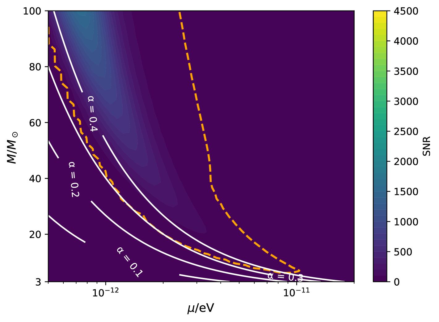
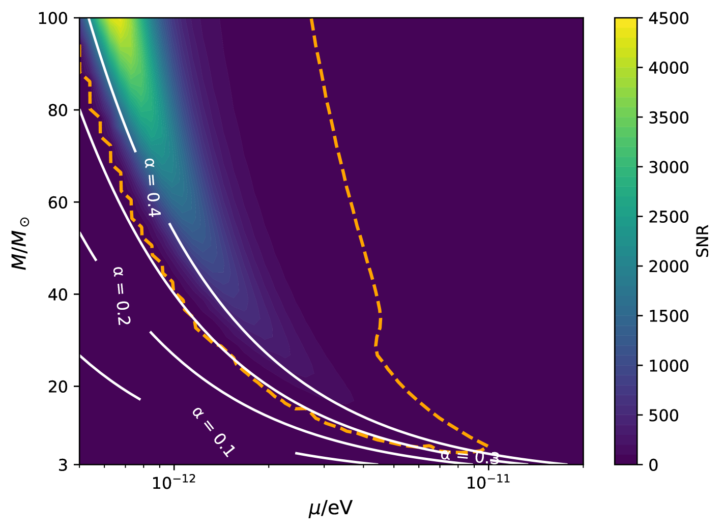
Figure 1: SNR of cloud level transition GWs observed in the deci-Hz band. We consider the hyperfine cloud level transition from $\ket{211}$ to $\ket{21-1}$, assuming a scalar field of mass $\mu$ and equal mass binaries with black holes of mass $M$ at redshift $z=0.01$. The cloud mass $M_{\rm c}$ is assumed to be $0.1M$. The upper panel shows the SNR of the GWs detected by DECIGO, and the lower panel shows that detected by BBO. The white lines show the contours of $\alpha$, which should be within $0.13<\alpha<0.42$ so that the clouds can fully grow and do not deplete before the level transition. The orange dashed lines show the contours of $\rho_{\rm SNR}=8$.

In addition, we consider intermediate mass black hole binaries, the corresponding level transition GWs are in milli-Hz band, cf. Eq. (17). Assuming a LISA-like detector [44], the SNR of the level transition GWs is shown in Fig. 2.

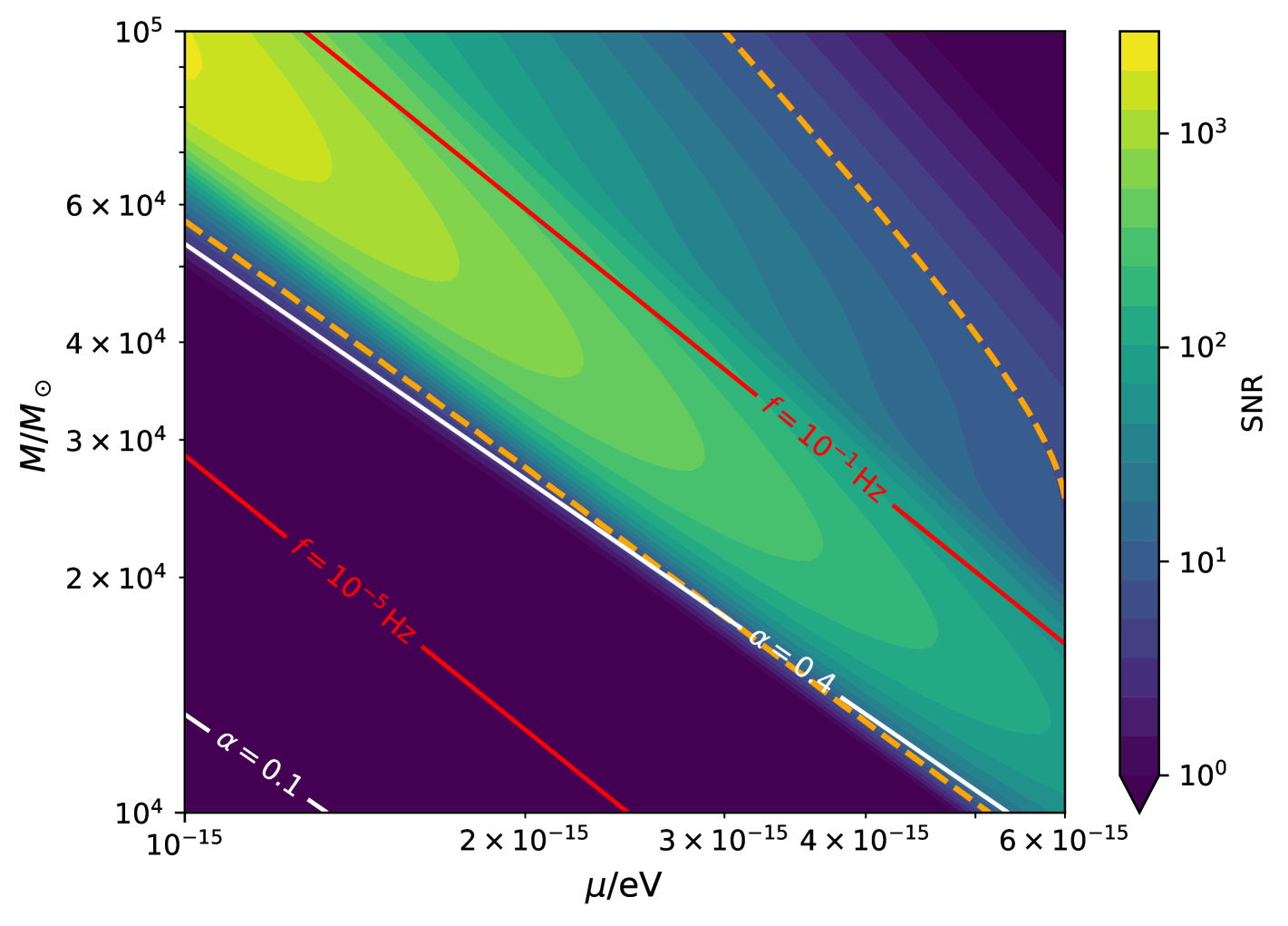
Figure 2: SNR of cloud level transition GWs observed in the milli-Hz band. We consider the hyperfine cloud level transition from $\ket{211}$ to $\ket{21-1}$, assuming a scalar field of mass $\mu$ and equal mass binaries with black holes of mass $M$ at redshift $z=0.1$ and detected by a LISA-like GW detector. The cloud mass $M_{\rm c}$ is assumed to be $0.1M$. The white lines show the contours of $\alpha$, which should be within $0.13<\alpha<0.42$ so that the clouds can fully grow and does not deplete before the level transition. The orange dashed line shows the contour of $\rho_{\rm SNR}=8$. The red lines show the characteristic frequency of the GW signals.

Given the SNR of cloud level transition GWs, we shall further estimate the rate of detectable events. For a certain scalar field of mass $\mu$, the event rate can be estimated by integrating all binary black hole merger events with $0.13<\alpha<0.42$ and with $\rho_{\rm SNR}\geq 8$,

$$R_{\rm lt}(\mu)=\int{\rm d}z\int_{M_{\rm min}(z)}^{M_{\rm max}(z)}{\rm d}MR_{\rm mrg}\left(M,t(z)\right)\frac{{\rm d}V_{c}}{{\rm d}z}\,,$$ (25)

where $\frac{{\rm d}V_{c}}{{\rm d}z}$ is differential comoving volume, $R_{\rm mrg}$ is the merger rate, and we have assumed all binaries are equal-mass for simplicity. The merger rate depends on the black hole formation history, and is computed following Ref. [45],

$$R_{{\rm mrg}}(M,t)=N\int_{\tau_{min}}^{\tau_{max}}d\tau_{\rm d}R_{\text{birth}}(M,t-\tau_{\rm d})P_{\rm d}(\tau_{\rm d})\,.$$ (26)

where $R_{\rm birth}(M,t)$ is the black hole birth rate at time $t$ and is normalized with the observed rate of $10^{-7}\rm{Mpc}^{-3}\rm{yr}^{-1}$ [46] to account for black holes that did not merge at all, $P_{\rm d}(\tau_{\rm d})\propto\tau_{\rm d}^{-1}$ is the distribution of time delay distribution, $\tau_{max}$ is the cosmic time, and $\tau_{min}$ is $50\text{Myr}$ or $\tau_{\rm lt}$, whichever is larger. In principle, $R_{{\rm mrg}}(M,t)$ might depend on the mass of field $\mu$. However, in the case that considered above, it always has $\tau_{\rm lt}<50\text{Myr}$, and thus $R_{{\rm mrg}}(M,t)$ does not depend on $\mu$. For concreteness, we consider black hole binaries formed via massive binary stars, in which case the black hole birth rate can be given by

$$R_{\text{birth}}(M,t(z))$$ (27)

$$= \int{\rm d}m_{\star}\,\text{SFR}(z)\,\text{IMF}(m_{\star})\,\delta(m_{\star}-g^{-1}(M,\mathcal{Z})).$$

Here, ${\rm SFR}(z)$ is the star formation rate [47], ${\rm IMF}(m_{\star})\propto m_{\star}^{-2.35}$ is the initial mass function [48], and $g(m_{\star},\mathcal{Z})$ is the relation between the remnant mass $M$ and the progenitor mass $m_{\star}$ [49] and also depends on the redshift through the metallicity $\mathcal{Z}$ [50].

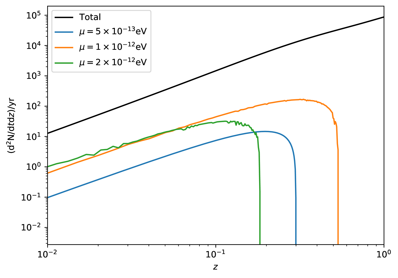
Figure 3: Event rate distribution of detectable cloud level transition GWs in redshift. We consider a BBO-like GW detector and a certain black hole population model, the merger rate of which is shown with the black line. The blue, orange, and green lines show the distributions assuming scalar fields of mass $0.5\times 10^{-12}{\rm eV}$, $1\times 10^{-12}{\rm eV}$, and $2\times 10^{-12}{\rm eV}$, and give a total event rate of $3{\rm yr}^{-1}$, $51{\rm yr}^{-1}$ and $3{\rm yr}^{-1}$ respectively.

Fig. 3 shows the event rate distribution of detectable cloud level transition GWs in redshift, assuming a BBO-like detector. We consider scalar fields of different masses, and find the distribution is maximized around $\mu=10^{-12}{\rm eV}$ with a total rate of $51$ events per year. For fields of larger masses, the event rate decreases due to the low SNR, while for fields of smaller mass, the event rate decreases due to the lack of heavy stellar mass black holes.

IV.2 Stochastic gravitational wave background

The cloud level transition GWs may also form stochastic gravitational wave background (SGWB). Given the black hole binary population, the energy density of SGWB can be calculated as

$$\Omega_{GW}(f_{o})=\frac{8\pi G}{3c^{2}H_{0}^{2}}f_{o}\int d\theta p(\theta)\int dz\frac{R_{\text{mrg}}(M,t(z))}{(1+z)E_{V}(z)}\frac{dE(\theta)}{df}.$$ (28)

where $f_{o}=f/(1+z)$ is observed frequency, $E_{V}(z)=\sqrt{\Omega_{m}(1+z)^{3}+\Omega_{\Lambda}}$ with $\Omega_{m}$ and $\Omega_{\Lambda}$ being the fractional energy density of dark matter and dark energy respectively, $\theta$ are source parameters, and $p(\theta)$ are the distributions thereof. $\frac{dE}{df}$ is the energy spectrum for a single event, and is generally given by

$$\frac{dE}{df}=\frac{\pi c^{3}}{2G}f^{2}r^{2}\int d\hat{\Omega}\left|\tilde{h}(f,\theta)\right|^{2}\,,$$ (29)

where the integral is over the solid angle $\hat{\Omega}$. In our case, $\frac{dE}{df}$ only depends on the black hole mass $M$ given a certain $\mu$, and the SGWB energy density is

$$\Omega_{GW}^{H}(f_{o})=\frac{8\pi G}{3c^{2}H_{0}^{2}}f_{o}\int{\rm d}M\int dz\frac{R_{\text{mrg}}(M,t(z))}{(1+z)E_{V}(z)}\frac{dE(M)^{\rm H}_{211}}{df}\,.$$ (30)

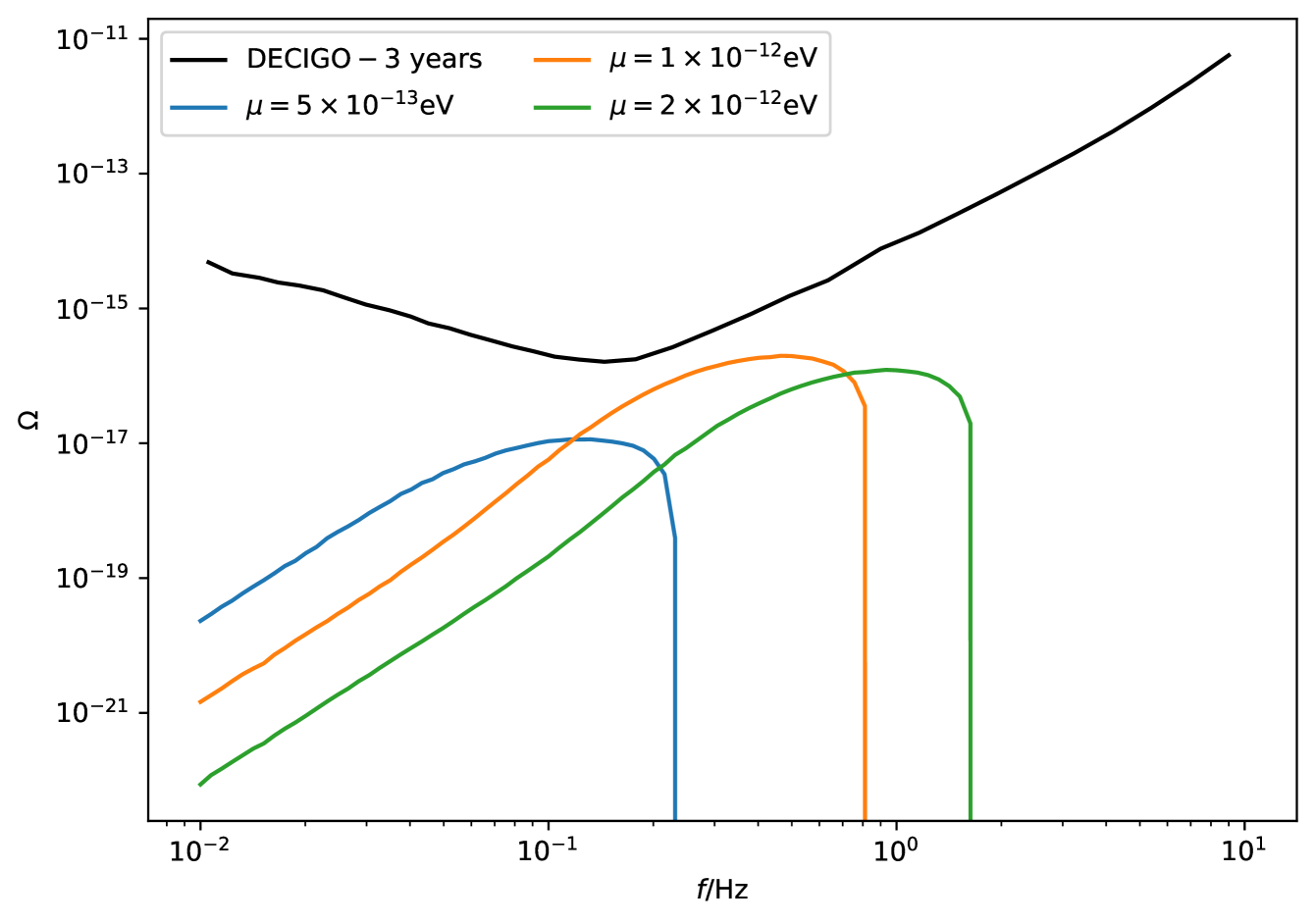
Figure 4: Energy density of the cloud level transition SGWB. We consider the hyperfine level transition between $\ket{21\pm 1}$, and show the energy density of the cloud level transition SGWB of scalar fields with $\mu=0.5\times 10^{-12}{\rm eV}$ (in blue), $1\times 10^{-12}{\rm eV}$ (in orange), and $2\times 10^{-12}{\rm eV}$ (in green). The black line demonstrates the correlated sensitivity of DECIGO for 3 years observation [51].

Considering scalar fields of mass $\mu=0.5\times 10^{-12}{\rm eV}$, $1\times 10^{-12}{\rm eV}$, and $2\times 10^{-12}{\rm eV}$, the energy density of SGWB from the cloud level transition is shown in Fig. 4. We find that the SGWB can not be detected by DECIGO with 3-year observation.

V Conclusion and Discussion

The detection of GWs opens up a new window to the dark sector of our universe, and have already demonstrated its potential in probing fundamental physics, e.g., see Refs. [12, 13, 14, 15, 16, 17, 18, 52, 53, 54, 55, 56, 57]. In this work, we investigate the possibility of probing ultralight bosons with the GW signals produced in their cloud level transitions. By explicitly calculating the cloud level transition GWs, we find that, for clouds that are initially in $\ket{211}$, the hyperfine level transition can lead to quadrupole GW radiation, while fine and Bohr level transitions do not lead to significant GW radiation. Focusing on the hyperfine level transition between $\ket{21\pm 1}$, we find that the resulting GWs is around $0.1$Hz for stellar mass black hole binaries, and around $10^{-3}$ Hz for intermediate mass black hole binaries. We further investigate the detectability of such GWs with GW detectors such as DECIGO, BBO and LISA, and find that BBO could detect such GW signals at rate of 51 events per year if there is a scalar field with mass around $10^{-12}$ eV. We also compute the energy density of cloud level transition SGWB, which however cannot be detected by DECIGO, assuming a 3-year observation. Our study forecasts the detectability of the cloud level transition GWs, and demonstrates such signals could be detected by a BBO-like detector, providing a potential way of probing ultralight boson with mass around $10^{-12}$eV. While ultralight fields can also be probed by the quasi-monochromic GWs emitted by clouds around isolated black holes, observing the cloud level transition GWs can help breaking the degeneracy, distinguishing the clouds from other GW sources.

While in this work we focus on the cloud level transition GWs, it is known that superradiant clouds in binaries also produce other observational signatures. In particular, the presence of clouds in binaries can alter the orbital dynamics, e.g., leading to floating and sinking orbits. These effects could also be detected by observing GWs produced by the binaries, providing another smoking gun for the existence of the clouds and hence the corresponding ultralight fields. It is also demonstrated in Ref. [58], these effects can be probed with multi-band GW observations, even without the direct detections of GWs during the resonant transitions. The prospects of probing the superradiant clouds with multi-band GW observations and with combination of all their signatures could be interesting, and are left for future studies.

Appendix A Detailed calculation of GW radiations from cloud level transitions

In this Appendix, we calculate the GWs radiation from cloud level transition with the multipole expansion method. We shall start with the stress-energy tensor of the complex scalar $\Psi$

$$T_{\mu\nu}={\Psi^{*}_{,(\mu}}\Psi_{,\nu)}-\frac{1}{2}g_{\mu\nu}(\Psi^{*}_{,\alpha}\Psi^{,\alpha}+\mu^{2}\Psi^{*}\Psi)\,.$$ (31)

In Newtonian approximation, the stress-energy tensor is dominated by ${T^{0}}_{0}\approx\mu|\Psi|^{2}$. In the two-state model, we have

$$\Psi=c_{1}(t)\Psi_{1}+c_{2}(t)\Psi_{2}\,,$$ (32)

where $c_{1}$ and $c_{2}$ describe the Landau-Zener transition, and $\Psi$ is normalized with $\int{\rm d}x^{3}|\Psi|^{2}=M_{\rm c}/\mu$. $\Psi$ can be rewritten as

$$\Psi=\frac{M_{\rm c}}{\mu}\left(c_{1}\psi_{1}e^{-i\epsilon_{1}t}+c_{2}\psi_{2}e^{-i\epsilon_{2}t}\right)\,,$$ (33)

where modes $\psi_{1}$ and $\psi_{2}$ are normalized as $\int{\rm d}x^{3}|\psi_{1}|^{2}=\int{\rm d}x^{3}|\psi_{2}|^{2}=1$, and $M_{\rm c}$ is the mass of the cloud. Then, the multipole of the cloud is

$$I_{lm}=\frac{16\pi\mu}{(2l+1)!!}\left[\frac{(l+1)(l+2)}{2l(l-1)}\right]^{1/2}\int{\rm d}^{3}x\,r^{l}|\Psi|^{2}Y^{*}_{lm},$$ (34)

where $Y_{lm}$ is the spherical Harmonics. Given the multipole of the cloud, one can define

$$u_{lm}=\frac{d^{l}}{dt^{l}}I_{lm},$$ (35)

and the GWs radiated by the cloud, in the transverse-traceless gauge, is

$$h_{ij}=\frac{G}{r}\sum_{l=2}^{\infty}\sum_{m=-l}^{l}u_{lm}\mathbf{T}^{lm}_{ij}(\theta,\phi),$$ (36)

where $\mathbf{T}^{lm}_{ij}(\theta,\phi)=\left(2\frac{(l-2)!}{(l+2)!}\right)^{1/2}r^{2}\Lambda_{ij,i^{\prime}j^{\prime}}(\hat{n})\partial_{i^{\prime}}\partial_{j^{\prime}}Y_{lm}(\theta,\phi)$ is the base of the metric perturbation, with $\Lambda_{ij,i^{\prime}j^{\prime}}$ being the projection tensor, $\hat{n}$ being the direction of the propagation of gravitational waves, and $i,j,i^{\prime},j^{\prime}$ denoting the Cartesian bases.

GWs from cloud level transition can be written as two parts, $h_{ij}=h_{ij}^{\Sigma}+h_{ij}^{\Pi}$, where $h_{ij}^{\Sigma}$ is sourced by $c_{1}^{2}|\Psi_{1}|^{2}+c_{2}^{2}|\Psi_{2}|^{2}$, and $h_{ij}^{\Pi}$ is sourced by $c_{1}^{*}c_{2}\Psi_{1}^{*}\Psi_{2}+c.c.$. Focusing on the quadrupole GW radiation, the explicit expression are given by

$$h^{\Sigma}_{ij}(t)= \frac{GM_{\rm c}}{c^{2}r}\left(\frac{GM}{c^{3}}\right)^{2}\alpha^{-4}$$ (37)

$$\times\left[C_{aa}2\eta^{2}\left(\tilde{c}_{b}(t)^{2}-\tilde{c}_{a}(t)^{2}\right)+\left(\eta\absolutevalue{\Delta m}\left(\dot{\phi}_{*}-\Omega_{0}\right)+i\dot{\eta}\right)\tilde{c}_{a}(t)\tilde{c}^{*}_{b}(t)+\left(\eta\absolutevalue{\Delta m}\left(\dot{\phi}_{*}-\Omega_{0}\right)-i\dot{\eta}\right)\ \tilde{c}_{b}(t)\tilde{c}^{*}_{a}(t)\right.$$

$$+\left.C_{bb}2\eta^{2}\left(\tilde{c}_{a}(t)^{2}-\tilde{c}_{b}(t)^{2}\right)+\left(\eta\absolutevalue{\Delta m}\left(\Omega_{0}-\dot{\phi}_{*}\right)-i\dot{\eta}\right)\tilde{c}_{a}(t)\tilde{c}^{*}_{b}(t)+\left(\eta\absolutevalue{\Delta m}\left(\Omega_{0}-\dot{\phi}_{*}\right)+i\dot{\eta}\right)\ \tilde{c}_{b}(t)\tilde{c}^{*}_{a}(t)\right]$$

$$\times\mathbf{T}^{lm}_{ij}(\theta,\phi)\mathcal{O}(\alpha),$$

and

$$h^{\Pi}_{ij}(t)= C_{ab}\frac{GM_{\rm c}}{c^{2}r}\left(\frac{GM}{c^{3}}\right)^{2}\alpha^{-4}$$ (38)

$$\times\left\{\left\{-e^{i(m_{b}-m_{a})\phi_{*}}\left[2(m_{a}-m_{b})\left((m_{a}-m_{b})+\Delta{m}\right)\dot{\phi}_{*}^{2}-2(m_{a}-m_{b})\left((m_{a}-m_{b})+\Delta{m}\right)\Omega_{0}\dot{\phi}_{*}\right.\right.\right.$$

$$\left.\left.+(m_{a}-m_{b})^{2}\Omega_{0}^{2}+i\left[\absolutevalue{\Delta m}(\dot{\phi}_{*}-\Omega_{0})/t+(m_{a}-m_{b})\ddot{\phi_{*}}\right]\right]+4\eta^{2}i\sin{[(m_{a}-m_{b})\phi_{*}]}\right\}\tilde{c}_{a}(t)\tilde{c}^{*}_{b}(t)$$

$$+\left\{-e^{i(m_{a}-m_{b})\phi_{*}}\left[2(m_{a}-m_{b})\left((m_{a}-m_{b})+\Delta{m}\right)\dot{\phi}_{*}^{2}-2(m_{a}-m_{b})\left((m_{a}-m_{b})+\Delta{m}\right)\Omega_{0}\dot{\phi}_{*}\right.\right.$$

$$\left.\left.+(m_{a}-m_{b})^{2}\Omega_{0}^{2}-i\left[\absolutevalue{\Delta m}(\dot{\phi}_{*}-\Omega_{0})/t+(m_{a}-m_{b})\ddot{\phi_{*}}\right]\right]-4\eta^{2}i\sin{[(m_{a}-m_{b})\phi_{*}]}\right\}\tilde{c}_{b}(t)\tilde{c}^{*}_{a}(t)$$

$$+2\left\{\left[\eta\left(2(m_{a}-m_{b})\dot{\phi}_{*}+\absolutevalue{\Delta m}(\dot{\phi}_{*}-\Omega_{0})\right)\right]\cos{[(m_{a}-m_{b})\phi_{*}]}-i\dot{\eta}\sin{[(m_{a}-m_{b})\phi_{*}]}\right\}\tilde{c}_{a}(t)\tilde{c}^{*}_{a}(t)$$

$$\left.-2\left\{\left[\eta\left(2(m_{a}-m_{b})\dot{\phi}_{*}+\absolutevalue{\Delta m}(\dot{\phi}_{*}-\Omega_{0})\right)\right]\cos{[(m_{a}-m_{b})\phi_{*}]}-i\dot{\eta}\sin{[(m_{a}-m_{b})\phi_{*}]}\right\}\tilde{c}_{b}(t)\tilde{c}^{*}_{b}(t)\right\}$$

$$\times\mathbf{T}^{lm}_{ij}(\theta,\phi)+\mathcal{O}(\alpha),$$

where $\tilde{c}_{a},\tilde{c}_{b}$ are expressions for $c_{a},c_{b}$ in the dressed frame, and

$$C_{ab} =\frac{128\sqrt{3}\pi}{15\sqrt{n_{a}^{3}n_{b}^{3}l_{a}l_{b}}}\sum_{k=0}^{n_{a}-l_{a}-1}\sum_{p=0}^{n_{b}-l_{b}-1}\frac{(-1)^{k+p}2^{l_{a}+l_{b}+k+p}}{k!p!}\frac{n_{a}^{5+l_{b}+p}n_{b}^{5+l_{a}+k}}{(n_{a}+n_{b})^{5+l_{a}+l_{b}+k+p}}\Gamma(5+l_{a}+l_{b}+k+p)$$ (39)

$$\times\sqrt{\frac{5(2l_{a}+1)(2l_{b}+1)}{4\pi}}\binom{n_{a}+l_{a}}{n_{a}-l_{a}-1-k}\binom{n_{b}+l_{b}}{n_{b}-l_{b}-1-p}\begin{pmatrix}2&l_{a}&l_{b}\\ 0&0&0\end{pmatrix}\begin{pmatrix}2&l_{a}&l_{b}\\ m_{a}-m_{b}&-m_{a}&m_{b}\end{pmatrix}.$$

We also show the explicit expression of octupole GW radiation. Assuming $\Omega_{0}\gg\eta$ and $\Omega_{0}\gg\gamma^{1/2}$, the leading term of octupole GW radiation is

$$h_{ij}(t) =\frac{256\sqrt{15}\pi}{315\sqrt{n_{a}^{3}n_{b}^{3}l_{a}l_{b}}}\sum_{k=0}^{n_{a}-l_{a}-1}\sum_{p=0}^{n_{b}-l_{b}-1}\frac{(-1)^{k+p}2^{l_{a}+l_{b}+k+p}}{k!p!}\frac{n_{a}^{6+l_{b}+p}n_{b}^{6+l_{a}+k}}{(n_{a}+n_{b})^{6+l_{a}+l_{b}+k+p}}\Gamma(6+l_{a}+l_{b}+k+p)$$ (40)

$$\times\sqrt{\frac{7(2l_{a}+1)(2l_{b}+1)}{4\pi}}\binom{n_{a}+l_{a}}{n_{a}-l_{a}-1-k}\binom{n_{b}+l_{b}}{n_{b}-l_{b}-1-p}\begin{pmatrix}3&l_{a}&l_{b}\\ 0&0&0\end{pmatrix}\begin{pmatrix}3&l_{a}&l_{b}\\ m_{a}-m_{b}&-m_{a}&m_{b}\end{pmatrix}$$

$$\times\frac{GM_{\rm c}}{c^{2}r}\left(\frac{GM\Omega_{0}}{c^{3}}\right)^{3}\alpha^{-5}(m_{a}-m_{b})^{3}\sin{[(m_{b}-m_{a})\phi_{*}]}\left(\tilde{c}_{a}(t)\tilde{c}^{*}_{b}(t)+\tilde{c}_{b}(t)\tilde{c}^{*}_{a}(t)\right)\mathbf{T}^{lm}_{ij}(\theta,\phi)+\mathcal{O}(\alpha).$$

References

- Arvanitaki et al. [2010] A. Arvanitaki, S. Dimopoulos, S. Dubovsky, N. Kaloper, and J. March-Russell, String Axiverse, Phys. Rev. D 81, 123530 (2010), arXiv:0905.4720 [hep-th] .
- Turner [1983] M. S. Turner, Coherent Scalar Field Oscillations in an Expanding Universe, Phys. Rev. D 28, 1243 (1983).
- Press et al. [1990] W. H. Press, B. S. Ryden, and D. N. Spergel, Single Mechanism for Generating Large Scale Structure and Providing Dark Missing Matter, Phys. Rev. Lett. 64, 1084 (1990).
- Hu et al. [2000] W. Hu, R. Barkana, and A. Gruzinov, Cold and fuzzy dark matter, Phys. Rev. Lett. 85, 1158 (2000), arXiv:astro-ph/0003365 .
- Amendola and Barbieri [2006] L. Amendola and R. Barbieri, Dark matter from an ultra-light pseudo-Goldsone-boson, Phys. Lett. B 642, 192 (2006), arXiv:hep-ph/0509257 .
- Schive et al. [2014] H.-Y. Schive, T. Chiueh, and T. Broadhurst, Cosmic Structure as the Quantum Interference of a Coherent Dark Wave, Nature Phys. 10, 496 (2014), arXiv:1406.6586 [astro-ph.GA] .
- Hui et al. [2017] L. Hui, J. P. Ostriker, S. Tremaine, and E. Witten, Ultralight scalars as cosmological dark matter, Phys. Rev. D 95, 043541 (2017), arXiv:1610.08297 [astro-ph.CO] .
- Brito et al. [2015] R. Brito, V. Cardoso, and P. Pani, Superradiance: New Frontiers in Black Hole Physics, Lect. Notes Phys. 906, pp.1 (2015), arXiv:1501.06570 [gr-qc] .
- Arvanitaki et al. [2015] A. Arvanitaki, M. Baryakhtar, and X. Huang, Discovering the QCD Axion with Black Holes and Gravitational Waves, Phys. Rev. D 91, 084011 (2015), arXiv:1411.2263 [hep-ph] .
- Brito et al. [2017a] R. Brito, S. Ghosh, E. Barausse, E. Berti, V. Cardoso, I. Dvorkin, A. Klein, and P. Pani, Stochastic and resolvable gravitational waves from ultralight bosons, Phys. Rev. Lett. 119, 131101 (2017a), arXiv:1706.05097 [gr-qc] .
- Brito et al. [2017b] R. Brito, S. Ghosh, E. Barausse, E. Berti, V. Cardoso, I. Dvorkin, A. Klein, and P. Pani, Gravitational wave searches for ultralight bosons with LIGO and LISA, Phys. Rev. D 96, 064050 (2017b), arXiv:1706.06311 [gr-qc] .
- Tsukada et al. [2019] L. Tsukada, T. Callister, A. Matas, and P. Meyers, First search for a stochastic gravitational-wave background from ultralight bosons, Phys. Rev. D 99, 103015 (2019), arXiv:1812.09622 [astro-ph.HE] .
- Isi et al. [2019] M. Isi, L. Sun, R. Brito, and A. Melatos, Directed searches for gravitational waves from ultralight bosons, Phys. Rev. D 99, 084042 (2019), [Erratum: Phys.Rev.D 102, 049901 (2020)], arXiv:1810.03812 [gr-qc] .
- Palomba et al. [2019] C. Palomba et al., Direct constraints on ultra-light boson mass from searches for continuous gravitational waves, Phys. Rev. Lett. 123, 171101 (2019), arXiv:1909.08854 [astro-ph.HE] .
- Tsukada et al. [2021] L. Tsukada, R. Brito, W. E. East, and N. Siemonsen, Modeling and searching for a stochastic gravitational-wave background from ultralight vector bosons, Phys. Rev. D 103, 083005 (2021), arXiv:2011.06995 [astro-ph.HE] .
- Ng et al. [2021] K. K. Y. Ng, S. Vitale, O. A. Hannuksela, and T. G. F. Li, Constraints on Ultralight Scalar Bosons within Black Hole Spin Measurements from the LIGO-Virgo GWTC-2, Phys. Rev. Lett. 126, 151102 (2021), arXiv:2011.06010 [gr-qc] .
- Abbott et al. [2022] R. Abbott et al. (LIGO Scientific, Virgo, KAGRA), All-sky search for gravitational wave emission from scalar boson clouds around spinning black holes in LIGO O3 data, Phys. Rev. D 105, 102001 (2022), arXiv:2111.15507 [astro-ph.HE] .
- Yuan et al. [2022] C. Yuan, Y. Jiang, and Q.-G. Huang, Constraints on an ultralight scalar boson from Advanced LIGO and Advanced Virgo’s first three observing runs using the stochastic gravitational-wave background, Phys. Rev. D 106, 023020 (2022), arXiv:2204.03482 [astro-ph.CO] .
- Miller [2025] A. L. Miller, Gravitational wave probes of particle dark matter: a review, (2025), arXiv:2503.02607 [astro-ph.HE] .
- Baumann et al. [2019] D. Baumann, H. S. Chia, and R. A. Porto, Probing Ultralight Bosons with Binary Black Holes, Phys. Rev. D 99, 044001 (2019), arXiv:1804.03208 [gr-qc] .
- Baumann et al. [2020] D. Baumann, H. S. Chia, R. A. Porto, and J. Stout, Gravitational Collider Physics, Phys. Rev. D 101, 083019 (2020), arXiv:1912.04932 [gr-qc] .
- Berti et al. [2019] E. Berti, R. Brito, C. F. B. Macedo, G. Raposo, and J. L. Rosa, Ultralight boson cloud depletion in binary systems, Phys. Rev. D 99, 104039 (2019), arXiv:1904.03131 [gr-qc] .
- Ikeda et al. [2021] T. Ikeda, L. Bernard, V. Cardoso, and M. Zilhão, Black hole binaries and light fields: Gravitational molecules, Phys. Rev. D 103, 024020 (2021), arXiv:2010.00008 [gr-qc] .
- Choudhary et al. [2021] S. Choudhary, N. Sanchis-Gual, A. Gupta, J. C. Degollado, S. Bose, and J. A. Font, Gravitational waves from binary black hole mergers surrounded by scalar field clouds: Numerical simulations and observational implications, Phys. Rev. D 103, 044032 (2021), arXiv:2010.00935 [gr-qc] .
- Tong et al. [2022] X. Tong, Y. Wang, and H.-Y. Zhu, Termination of superradiance from a binary companion, Phys. Rev. D 106, 043002 (2022), arXiv:2205.10527 [gr-qc] .
- Baumann et al. [2022a] D. Baumann, G. Bertone, J. Stout, and G. M. Tomaselli, Ionization of gravitational atoms, Phys. Rev. D 105, 115036 (2022a), arXiv:2112.14777 [gr-qc] .
- Guo et al. [2024] A. Guo, J. Zhang, and H. Yang, Superradiant clouds may be relevant for close compact object binaries, Phys. Rev. D 110, 023022 (2024), arXiv:2401.15003 [gr-qc] .
- Liu [2024] J. Liu, Gravitational laser: the stimulated radiation of gravitational waves from the clouds of ultralight bosons, (2024), arXiv:2401.16096 [gr-qc] .
- Cardoso et al. [2011] V. Cardoso, S. Chakrabarti, P. Pani, E. Berti, and L. Gualtieri, Floating and sinking: The Imprint of massive scalars around rotating black holes, Phys. Rev. Lett. 107, 241101 (2011), arXiv:1109.6021 [gr-qc] .
- Ferreira et al. [2017] M. C. Ferreira, C. F. B. Macedo, and V. Cardoso, Orbital fingerprints of ultralight scalar fields around black holes, Phys. Rev. D 96, 083017 (2017), arXiv:1710.00830 [gr-qc] .
- Zhang and Yang [2019] J. Zhang and H. Yang, Gravitational floating orbits around hairy black holes, Phys. Rev. D 99, 064018 (2019), arXiv:1808.02905 [gr-qc] .
- Zhang and Yang [2020] J. Zhang and H. Yang, Dynamic Signatures of Black Hole Binaries with Superradiant Clouds, Phys. Rev. D 101, 043020 (2020), arXiv:1907.13582 [gr-qc] .
- Baumann et al. [2022b] D. Baumann, G. Bertone, J. Stout, and G. M. Tomaselli, Sharp Signals of Boson Clouds in Black Hole Binary Inspirals, Phys. Rev. Lett. 128, 221102 (2022b), arXiv:2206.01212 [gr-qc] .
- Tomaselli et al. [2023] G. M. Tomaselli, T. F. M. Spieksma, and G. Bertone, Dynamical friction in gravitational atoms, JCAP 07, 070, arXiv:2305.15460 [gr-qc] .
- Cao and Tang [2023] Y. Cao and Y. Tang, Signatures of Ultralight Bosons in Compact Binary Inspiral and Outspiral, (2023), arXiv:2307.05181 [gr-qc] .
- Tomaselli et al. [2024a] G. M. Tomaselli, T. F. M. Spieksma, and G. Bertone, Resonant history of gravitational atoms in black hole binaries, Phys. Rev. D 110, 064048 (2024a), arXiv:2403.03147 [gr-qc] .
- Cao et al. [2024] Y. Cao, Y.-Z. Cheng, G.-L. Li, and Y. Tang, Probing vector gravitational atom with eccentric intermediate mass-ratio inspirals, (2024), arXiv:2411.17247 [gr-qc] .
- Takahashi et al. [2024] T. Takahashi, H. Omiya, and T. Tanaka, Self-interacting axion clouds around rotating black holes in binary systems, Phys. Rev. D 110, 104038 (2024), arXiv:2408.08349 [gr-qc] .
- Zhu et al. [2025] H.-Y. Zhu, X. Tong, G. Manzoni, and Y. Ma, Survival of the Fittest: Testing Superradiance Termination with Simulated Binary Black Hole Statistics, Astrophys. J. 981, 165 (2025), arXiv:2409.14159 [gr-qc] .
- Tomaselli et al. [2024b] G. M. Tomaselli, T. F. M. Spieksma, and G. Bertone, Legacy of Boson Clouds on Black Hole Binaries, Phys. Rev. Lett. 133, 121402 (2024b), arXiv:2407.12908 [gr-qc] .
- Bošković et al. [2024] M. Bošković, M. Koschnitzke, and R. A. Porto, Signatures of Ultralight Bosons in the Orbital Eccentricity of Binary Black Holes, Phys. Rev. Lett. 133, 121401 (2024), arXiv:2403.02415 [gr-qc] .
- Guo et al. [2023] Y. Guo, W. Zhong, Y. Ma, and D. Su, Mass transfer and boson cloud depletion in a binary black hole system, (2023), arXiv:2309.07790 [gr-qc] .
- Yagi and Seto [2011] K. Yagi and N. Seto, Detector configuration of DECIGO/BBO and identification of cosmological neutron-star binaries, Phys. Rev. D 83, 044011 (2011), [Erratum: Phys.Rev.D 95, 109901 (2017)], arXiv:1101.3940 [astro-ph.CO] .
- Robson et al. [2019] T. Robson, N. J. Cornish, and C. Liu, The construction and use of LISA sensitivity curves, Class. Quant. Grav. 36, 105011 (2019), arXiv:1803.01944 [astro-ph.HE] .
- Dvorkin et al. [2016] I. Dvorkin, E. Vangioni, J. Silk, J.-P. Uzan, and K. A. Olive, Metallicity-constrained merger rates of binary black holes and the stochastic gravitational wave background, Mon. Not. Roy. Astron. Soc. 461, 3877 (2016), arXiv:1604.04288 [astro-ph.HE] .
- Abbott et al. [2016] B. P. Abbott et al. (LIGO Scientific, Virgo), The Rate of Binary Black Hole Mergers Inferred from Advanced LIGO Observations Surrounding GW150914, Astrophys. J. Lett. 833, L1 (2016), arXiv:1602.03842 [astro-ph.HE] .
- Vangioni et al. [2015] E. Vangioni, K. A. Olive, T. Prestegard, J. Silk, P. Petitjean, and V. Mandic, The Impact of Star Formation and Gamma-Ray Burst Rates at High Redshift on Cosmic Chemical Evolution and Reionization, Mon. Not. Roy. Astron. Soc. 447, 2575 (2015), arXiv:1409.2462 [astro-ph.GA] .
- Salpeter [1955] E. E. Salpeter, The Luminosity function and stellar evolution, Astrophys. J. 121, 161 (1955).
- Woosley and Weaver [1995] S. E. Woosley and T. A. Weaver, The Evolution and explosion of massive stars. 2. Explosive hydrodynamics and nucleosynthesis, Astrophys. J. Suppl. 101, 181 (1995).
- Belczynski et al. [2016] K. Belczynski, D. E. Holz, T. Bulik, and R. O’Shaughnessy, The first gravitational-wave source from the isolated evolution of two 40-100 Msun stars, Nature 534, 512 (2016), arXiv:1602.04531 [astro-ph.HE] .
- Kawamura [2023] S. Kawamura (DECIGO working group), Space gravitational wave antenna DECIGO and B-DECIGO, PoS ICRC2023, 1516 (2023).
- Sagunski et al. [2018] L. Sagunski, J. Zhang, M. C. Johnson, L. Lehner, M. Sakellariadou, S. L. Liebling, C. Palenzuela, and D. Neilsen, Neutron star mergers as a probe of modifications of general relativity with finite-range scalar forces, Phys. Rev. D 97, 064016 (2018), arXiv:1709.06634 [gr-qc] .
- Huang et al. [2019] J. Huang, M. C. Johnson, L. Sagunski, M. Sakellariadou, and J. Zhang, Prospects for axion searches with Advanced LIGO through binary mergers, Phys. Rev. D 99, 063013 (2019), arXiv:1807.02133 [hep-ph] .
- Sennett et al. [2020] N. Sennett, R. Brito, A. Buonanno, V. Gorbenko, and L. Senatore, Gravitational-Wave Constraints on an Effective Field-Theory Extension of General Relativity, Phys. Rev. D 102, 044056 (2020), arXiv:1912.09917 [gr-qc] .
- Zhang et al. [2021] J. Zhang, Z. Lyu, J. Huang, M. C. Johnson, L. Sagunski, M. Sakellariadou, and H. Yang, First Constraints on Nuclear Coupling of Axionlike Particles from the Binary Neutron Star Gravitational Wave Event GW170817, Phys. Rev. Lett. 127, 161101 (2021), arXiv:2105.13963 [hep-ph] .
- Barsanti et al. [2023] S. Barsanti, A. Maselli, T. P. Sotiriou, and L. Gualtieri, Detecting Massive Scalar Fields with Extreme Mass-Ratio Inspirals, Phys. Rev. Lett. 131, 051401 (2023), arXiv:2212.03888 [gr-qc] .
- Liu et al. [2024] H.-Y. Liu, Y.-S. Piao, and J. Zhang, Probing higher-spin particles with gravitational waves from compact binary inspirals, Phys. Rev. D 109, 024030 (2024), arXiv:2302.08042 [gr-qc] .
- Chen et al. [2024] M.-C. Chen, H.-Y. Liu, Q.-Y. Zhang, and J. Zhang, Probing massive fields with multiband gravitational-wave observations, Phys. Rev. D 110, 064018 (2024), arXiv:2405.11583 [gr-qc] .
- Kyriazis and Yang [2025] A. Kyriazis and F. Yang, Gravitational Waves from Resonant Transitions of Tidally Perturbed Gravitational Atoms, (2025), arXiv:2503.18121 [hep-ph] .