A Fast Fourth-Order Cut Cell Method for Solving Elliptic Equations in Two-Dimensional Irregular Domains

Abstract

We propose a fast fourth-order cut cell method for solving constant-coefficient elliptic equations in two-dimensional irregular domains. In our methodology, the key to dealing with irregular domains is the poised lattice generation (PLG) algorithm that generates finite-volume interpolation stencils near the irregular boundary. We are able to derive high-order discretization of the elliptic operators by least squares fitting over the generated stencils. We then design a new geometric multigrid scheme to efficiently solve the resulting linear system. Finally, we demonstrate the accuracy and efficiency of our method through various numerical tests in irregular domains.

65D05, 65N08

1 Introduction

Consider the constant-coefficient elliptic equation

(1) $$a\frac{\partial^{2}u}{\partial x_{1}^{2}}+b\frac{\partial^{2}u}{\partial x_{1}\partial x_{2}}+c\frac{\partial^{2}u}{\partial x_{2}^{2}}=f\quad\text{in }\Omega,$$

where $u:\Omega\rightarrow\mathbb{R}$ is the unknown function, $a,b,c$ are real numbers satisfying $b^{2}-4ac<0$, and $\Omega$ is a open domain in $\mathbb{R}^{2}$. A particular case of interest is Poisson’s equation with $(a,b,c)=(1,0,1)$. Poisson’s equation plays an important role in many other mathematical formulations such as the Helmholtz decomposition and the projection methods [5, 12, 18, 29, 30] for solving the incompressible Navier-Stokes equations (INSE).

A myriad of efficient and accurate numerical methods have been developed for solving partial differential equations (PDEs) in rectangular domains. In many real-world applications, however, the problem domains are irregular with piecewise smooth boundaries. Different numerical methods have been proposed for irregular domains, including the notable finite element methods (FEM) on triangular meshes. Another approach is the cut cell method, in which the irregular domain is embedded into a background Cartesian mesh. One merit of the cut cell method is the relatively inexpensive grid generation and storage. Conventional unstructured or body-fitted grids require large computational memory for storing cells, faces and a connectivity table to link them. The Cartesian grid, on the other hand, does not need the storage of any connectivity table as they can be mapped by simple indices. As a result, the computational time is also reduced. Another merit is that mature techniques can be borrowed from the finite difference and finite volume community. Examples are multigrid algorithms [4] for elliptic equations, shock-capturing schemes [25, 21] for hyperbolic systems and high-order conservative schemes [23] for incompressible flows.

It is worth mentioning a class of finite difference Cartesian grid methods for the related “interface problems”. The Immersed Interface Method (IIM) [14, 15, 16, 17] modifies the discretization stencil to incorporate jump conditions on the interface. The Ghost Fluid Method (GFM) [20, 7, 19, 28] introduces ghost values as smooth extensions of the physical variables across the interface, so that conventional finite difference formulas can be employed.

For problems involving a single-phase fluid, the cut cell method (also known as Cartesian grid method and embedded boundary (EB) method) is preferred. Previously, second-order cut cell methods have been developed for Poisson’s equation [11, 24], heat equation [22, 24] and the Navier-Stokes equations [13, 27]. Recently, a fourth-order EB method for Poisson’s equation [6] was developed by Devendran et al. However, a number of issues presented in the cut cell method are only partially resolved, or even unresolved:

1. Given that the problem domains can be arbitrarily complex in geometry and topology, is there an accurate and efficient representation of such domains?

2. For domains with arbitrarily complex boundaries, the generation of cut cells and the stability issues arising from the small cells within them are intricate. Can we design a cutting algorithm to produce control volumes suitable for discretization?

3. Previously, the selection of stencils depended very much on both the order of discretization and the specific form of the differential operator. In these methods, obtaining a high-order discretization of the cross derivative term in complex geometries can be tricky. So can we generate stencils that adapt automatically to complex geometries, and meanwhile minimize their coupling with the high-order discretization of the differential operator?

4. Having discretized the elliptic equation, can we solve the resulting linear systems efficiently to produce fourth-order accurate solutions?

In this paper, we give positive answers to all the above questions by proposing a fast fourth-order cut cell method for solving constant-coefficient elliptic equations in two-dimensional irregular domains.

To answer (Q-1), we make use of the theory of Yin space [31]. The member of Yin space, called Yin set, is the mathematical model for physically meaningful regions in the plane. Every Yin set has a simple representation that facilitates geometric and topological queries. In this work, we will formulate the computational domains and the cut cells in terms of Yin sets. Our answer to (Q-2) relies on the Boolean operations equipped by the Yin space; see Theorem 2.3. We propose a systematic algorithm for generating cut cells and merging the small cells with volume fraction below a user-specified threshold in the computational domain. The key to answering (Q-3) is the poised lattice generation (PLG) algorithm [32]. Given a prescribed region of $\mathbb{Z}^{\scriptsize\textsf{D}}$, the PLG algorithm generates poised lattices on which multivariate polynomial interpolation is unisolvent. It has been successfully employed to obtain fourth- and sixth-order discretization of the convection operator in complex geometries. Based on the interpolation stencils, we demonstrate a general approach for deriving high-order approximations to linear differential operators, using least squares fitting by complete multivariate polynomials. This approach handles different boundary conditions and can be extended to nonlinear differential operators as well. To answer (Q-4), we design a new geometric multigrid algorithm for efficiently solving the resulting discrete linear system. We modify the conventional multigrid components to account for irregular domains and high-order discretization. We show by analysis and by numerical tests that the linear systems are solved with optimal complexity.

The rest of this paper is organized as follows. In Section 2 we collect preliminary concepts, with focus on the PLG algorithm in finite difference formulation. In Section 3, we propose a fourth-order cut cell method for constant-coefficient elliptic equations in irregular domains. Specifically, we discuss the cut-cell generation in Section 3.1, the standard finite-volume approximation in Section 3.2, the generation of finite-volume stencils near irregular boundaries, and the high-order discretization of the differential operators in Section 3.3. We then present a multigrid algorithm for efficiently solving the discrete linear system and analyze its complexity in Section 4. In Section 5, we perform numerical tests in various irregular domains to demonstrate the accuracy and efficiency of our method. Finally, we conclude this paper with some future research prospects in Section 6.

2 Preliminaries

In this section, we collect preliminary concepts that are necessary for the development of the proposed numerical method in this paper.

2.1 Yin space

To answer the need for an accurate and efficient representation of the irregular domains, we review a topological space for modeling physically meaningful regions.

Let $\mathcal{X}$ be a topological space, and $\mathcal{S},\mathcal{T}$ be two subsets of $\mathcal{X}$. Denote by $\mathcal{S}^{-}$ the closure of $\mathcal{S}$, and by $\mathcal{S}^{\perp}$ the exterior of $\mathcal{S}$, i.e. the interior of the complement of $\mathcal{S}$. A subset $\mathcal{S}$ is regular open if it coincides with the interior of its closure. Denote by $\cup^{\perp\perp}$ the regularized union operation, i.e. $\mathcal{S}\cup^{\perp\perp}\mathcal{T}:=\left(\mathcal{S}\cup\mathcal{T}\right)^{\perp\perp}$. It can be shown [8, §10] that the class of all regular open subsets of $\mathcal{X}$ is closed under the regularized union. For $\mathcal{X}=\mathbb{R}^{2}$, a subset $\mathcal{S}\subset\mathbb{R}^{2}$ is semianalytic if there exist a finite number of analytic functions $g_{i}:\mathbb{R}^{2}\rightarrow\mathbb{R}$ such that $\mathcal{S}$ is in the universe of a finite Boolean algebra formed from the sets

(2) $$\mathcal{X}_{i}=\left\{\mathbf{x}\in\mathbb{R}^{2}:g_{i}(\mathbf{x})\geq 0\right\}.$$

In particular, a semianalytic set is semialgebraic if all the $g_{i}$’s are polynomials.

Definition 2.1 (Yin Space [31]).

A Yin set $\mathcal{Y}\subset\mathbb{R}^{2}$ is a regular open semianalytic set whose boundary is bounded. The class of all such Yin sets form the Yin space $\mathbb{Y}$.

In the above definition, regularity captures the physical meaningfulness of the fluid regions, openness guarantees a unique boundary representation, and semianalyticity implies finite representation.

Definition 2.2.

The subspace $\mathbb{Y}_{\mathrm{c}}$ of $\mathbb{Y}$ consists of Yin sets whose boundaries are captured by cubic splines.

Theorem 2.3 (Zhang and Li [31]).

$\left(\mathbb{Y},\cup^{\perp\perp},\cap,^{\perp},\emptyset,\mathbb{R}^{2}\right)$ is a Boolean algebra.

Corollary 2.4.

$\mathbb{Y}_{\mathrm{c}}$ a sub-algebra of $\mathbb{Y}$.

Efficient algorithms have been developed in [31, Section 4] to implement the Boolean operations in Theorem 2.3. In this work, they will be used for cut cell generation and merging.

Consider the representation of a Yin set. If $\gamma$ is an oriented Jordan curve, denote by $\operatorname{int}(\gamma)$ the complement of $\gamma$ that always lies at the left of an observer who traverses $\gamma$ according to its orientation. It is shown in [31, Corollary 3.13] that every Yin set $\mathcal{Y}\neq\emptyset,\mathbb{R}^{2}$ can be uniquely expressed as

(3) $$\mathcal{Y}=\bigcup_{j}{}^{\perp\perp}\bigcap_{i}\operatorname{int}(\gamma_{j,i}),$$

where for each fixed $j$ the collection of oriented Jordan curves $\{\gamma_{j,i}\}_{i}$ is pairwise almost disjoint and corresponds to a connected component of $\mathcal{Y}$. The whole collection $\{\gamma_{j,i}\}$ can be further arranged in a fashion such that the topological information (such as Betti numbers) can be easily extracted within constant time; see [31, Definition 3.17].

2.2 Poised lattice generation

Traditional finite difference (FD) methods have limited applications in irregular domains, as they often replace the spatial derivatives in partial differential equations by one-dimensional FD formulas or their tensor-product counterparts. To overcome this limitation, the PLG algorithm [32] was proposed to generate poised lattices in complex geometries. Once the interpolation lattices have been generated, high-order discretization of the differential operators can be obtained via multivariate polynomial fitting.

In this section we give a brief review of the PLG problem. We begin with the relevant notions in multivariate interpolation.

Definition 2.5 (Lagrange interpolation problem (LIP)).

Denote by $\Pi_{n}^{{\scriptsize\textsf{D}}}$ the vector space of all D-variate polynomials of degree no more than $n$ with real coefficients. Given a finite number of points $\mathbf{x}_{1},\mathbf{x}_{2},\cdots,\mathbf{x}_{N}\in\mathbb{R}^{\scriptsize\textsf{D}}$ and the same number of data $f_{1},f_{2},\cdots,f_{N}\in\mathbb{R}$, the Lagrange interpolation problem seeks a polynomial $f\in\Pi_{n}^{\scriptsize\textsf{D}}$ such that

(4) $$f(\mathbf{x}_{j})=f_{j},\quad\forall j=1,2,\cdots,N,$$

where $\Pi_{n}^{\scriptsize\textsf{D}}$ is the interpolation space and $\mathbf{x}_{j}$’s the interpolation sites.

The sites $\left\{\mathbf{x}_{j}\right\}_{j=1}^{N}$ are said to be poised in $\Pi_{n}^{\scriptsize\textsf{D}}$ if there exists a unique $f\in\Pi_{n}^{\scriptsize\textsf{D}}$ satisfying (4) for any given data $\left\{f_{j}\right\}_{j=1}^{N}$. Suppose $\left\{\phi_{j}\right\}$ is a basis of $\Pi_{n}^{\scriptsize\textsf{D}}$. It is easy to see that the interpolation sites are poised if and only if $N=\dim\Pi_{n}^{\scriptsize\textsf{D}}=\binom{n+{\scriptsize\textsf{D}}}{n}$ and the $N\times N$ sample matrix

(5) $$M(\left\{\phi_{j}\right\};\left\{\mathbf{x}_{k}\right\})=\Big{[}M_{jk}\Big{]}:=\Big{[}\phi_{j}(\mathbf{x}_{k})\Big{]}\quad(1\leq j,k\leq N)$$

is non-singular.

Definition 2.6 (PLG in $\mathbb{Z}^{\scriptsize\textsf{D}}$ [32]).

Given a finite set of feasible nodes $K\in\mathbb{Z}^{\text{D}}$, a starting point $\mathbf{q}\in K$, and a degree $n\in\mathbb{Z}^{+}$, the problem of poised lattice generation is to choose a lattice $\mathcal{T}\subset K$ such that $\mathcal{T}$ is poised in $\Pi_{n}^{\scriptsize\textsf{D}}$ and $\#\mathcal{T}=\dim\Pi_{n}^{\scriptsize\textsf{D}}$.

In [32], we proposed a novel and efficient PLG algorithm to solve the PLG problem via an interdisciplinary research of approximation theory, abstract algebra, and artificial intelligence. The stencils are based on the transformation of the principal lattice. In this work, we directly apply the algorithm to our finite volume discretization. The starting point $\mathbf{q}$ corresponds to the cell index at which the spatial operators are discretized, and the feasible nodes $K$ formed by collecting the indices of nearby cut cells.

In general cases it is still unclear that whether a direct application of the PLG algorithm will generate poised stencils in finite volume formulation. Finding a strict proof of poisedness will be a topic of our future research. Nevertheless, the poisedness in finite volume formulation is supported by the extensive numerical evidences. For example, the condition numbers of the $({\scriptsize\textsf{D}},n)=(2,4)$ lattices used in this paper generally do not exceed $10^{4}$ in all problems of interest.

2.3 Least squares problems

To derive the approximation to the differential operators, we need the following results on weighted least squares fitting.

Definition 2.7.

For a symmetric positive definite matrix $W\in\mathbb{R}^{n\times n}$, the $W$-inner product is

(6) $$\langle u,v\rangle_{W}:=u^{T}Wv$$

and the $W$-norm is

(7) $$\|u\|_{W}:=\langle u,u\rangle_{W}^{1/2}$$

for $u,v\in\mathbb{R}^{n}$.

Proposition 2.8.

Let $A\in\mathbb{R}^{m\times n}$ be a matrix with full column rank, and let $W\in\mathbb{R}^{m\times m}$ be a symmetric positive definite matrix.

1. For any $b\in\mathbb{R}^{m}$, the optimization problem

   (8) $$\min_{x\in\mathbb{R}^{n}}\left\|Ax-b\right\|_{W}$$

   admits a unique solution $x_{\mathrm{LS}}=\left(A^{T}WA\right)^{-1}A^{T}Wb$.

2. For any $d\in\mathbb{R}^{n}$, the constrained optimization problem

   (9) $$\min_{x\in\mathbb{R}^{m}}\left\|x\right\|_{W^{-1}}\quad\mathrm{s.t.}\quad A^{T}x=d$$

   admits a unique solution $x_{\mathrm{NM}}=WA\left(A^{T}WA\right)^{-1}d$.

Proof 2.9.

See [9, §5.3, §5.6, §6.1].

2.4 Numerical cubature

In finite volume discretization, we need to evaluate the volume integral of a given function $f(x,y)$ over a control volume $\mathcal{C}\in\mathbb{Y}_{\mathrm{c}}$. For this purpose, we invoke the Green’s formula to convert

(10) $$\iint_{\mathcal{C}}f(x,y)\mathrm{d}x\mathrm{d}y=\oint_{\partial\mathcal{C}}F(x,y)\mathrm{d}y$$

into a line integral, where $\partial\mathcal{C}$ is the boundary of $\mathcal{C}$ and $F(x,y)=\int_{\xi_{0}}^{x}f(\xi,y)\mathrm{d}\xi$ is a primitive of $f(x,y)$ with respect to $x$, with $\xi_{0}$ an arbitrary fixed real number. Suppose $\left(x(t),y(t)\right)\left(t\in[0,1]\right)$ is a smooth parametrization of $\partial\mathcal{C}$. Then we can write

(11a) $$\oint_{\partial\mathcal{C}}F(x,y)\mathrm{d}y =\int_{0}^{1}F(x(t),y(t))\dot{y}(t)\mathrm{d}t$$

(11b) $$=\int_{0}^{1}\dot{y}(t)\int_{\xi_{0}}^{x(t)}f(\xi,y(t))\mathrm{d}\xi\mathrm{d}t,$$

into a two-fold iterated integral. The integral (11b) can be evaluated using one-dimensional numerical quadratures such as Gauss-Legendre quadrature. If the boundary $\partial\mathcal{C}$ is only piecewise smooth, we simply apply (11b) to each piece and sum up the results. If the integrand $f(x,y)$ is a bivariate polynomial, then (11b) expands to a (possibly very high-order) polynomial of $t$ whose coefficients depend on the parametrization $\left(x(t),y(t)\right)$ and the integrand $f(x,y)$. This polynomial can then be evaluated to machine precision without quadratures.

Although $\xi_{0}$ can be arbitrary, it should be selected to minimize round-off errors. A typical choice is the center of the bounding box of $\mathcal{C}$. See [26] for a detailed error analysis on using Gauss-Legendre quadrature to evaluate the cubature formula (11b).

3 Spatial discretization

3.1 Cut-cell generation

Let $R$ be a rectangular region containing $\Omega\in\mathbb{Y}_{\mathrm{c}}$ and partitioned uniformly into a collection of rectangular cells

(12) $$\mathrm{C}_{\mathbf{i}}:=\Big{(}\mathbf{i}h,(\mathbf{i}+\mathbbm{1})h\Big{)},$$

where $h$ is the uniform spatial step size, $\mathbf{i}\in\mathbb{Z}^{{\scriptsize\textsf{D}}}$ a multi-index, and $\mathbbm{1}\in\mathbb{Z}^{{\scriptsize\textsf{D}}}$ the multi-index with all its components equal to one. The higher face of the cell $\mathrm{C}_{\mathbf{i}}$ in dimension $d$ is denoted by

(13) $$\mathrm{F}_{\mathbf{i}+\frac{1}{2}\bm{\mathrm{e}}^{d}}:=\Big{(}(\mathbf{i}+\bm{\mathrm{e}}^{d})h,(\mathbf{i}+\mathbbm{1})h\Big{)},$$

where $\bm{\mathrm{e}}^{d}\in\mathbb{Z}^{\scriptsize\textsf{D}}$ is the multi-index with 1 as its $d$th component ($1\leq d\leq{\scriptsize\textsf{D}}$) and 0 otherwise. The cut cell method embeds the irregular domain $\Omega$ into the rectangular grid $R$. We define the cut cells by

(14) $$\mathcal{C}_{\mathbf{i}}:=\mathrm{C}_{\mathbf{i}}\cap\Omega,$$

the cut faces by

(15) $$\mathcal{F}_{\mathbf{i}+\frac{1}{2}\bm{\mathrm{e}}^{d}}:=\mathrm{F}_{\mathbf{i}+\frac{1}{2}\bm{\mathrm{e}}^{d}}\cap\Omega,$$

and the portion of domain boundary contained in a cut cell by

(16) $$\mathcal{S}_{\mathbf{i}}:=\mathrm{C}_{\mathbf{i}}\cap\partial\Omega.$$

A cut cell is said to be an empty cell if $\mathcal{C}_{\mathbf{i}}=\emptyset$, a pure cell if $\mathcal{C}_{\mathbf{i}}=\mathrm{C}_{\mathbf{i}}$, or an interface cell otherwise. In practice, cut cells may be arbitrarily small and the elliptic operator will be very ill-conditioned. A number of approaches have been proposed to address this problem: for example, the application of cell merging [10], the utilization of redistribution [1], or the formulation of special differencing schemes for the discretization [2]. Of these various approaches, we choose to use a simple cell-merging methodology to circumvent the small-cell problem.

Algorithm 1 Cut-cell generation and merging.

1:a computational domain $\Omega\in\mathbb{Y}_{c}$; a Cartesian grid with step size $h$; a user-specified threshold $\theta\in(0,1)$.

2:a set of cut cells $\left\{\mathcal{C}_{\mathbf{i}}\right\}_{\mathbf{i}\in\mathbb{Z}^{{\scriptsize\textsf{D}}}}$.

3:$\bigcup^{\bot\bot}_{\mathbf{i}}\mathcal{C}_{\mathbf{i}}=\Omega$ and the volume of each cut cell is not less than $\theta h^{2}$.

4:$\left\{\mathcal{C}_{\mathbf{i}}\right\}_{\mathbf{i}\in\mathbb{Z}^{{\scriptsize\textsf{D}}}}\leftarrow\left\{\mathrm{C}_{\mathbf{i}}\cap\Omega\right\}_{\mathbf{i}\in\mathbb{Z}^{{\scriptsize\textsf{D}}}}$ : the set of cut cells obtained by embedding $\Omega$ into the Cartesian grid.

5:Preprocess the cut cells $\mathcal{C}_{\mathbf{i}}=\left(\bigcup^{\bot\bot}\mathcal{C}_{\mathbf{i}}^{k}\right)_{k=1}^{n_{c}}$ with $n_{c}(n\geq 2)$ connected components by

$$\mathcal{C}_{\mathbf{i}}\leftarrow\mathcal{C}_{\mathbf{i}}^{m},\quad\mathcal{C}_{\mathbf{j}}\leftarrow\mathcal{C}_{\mathbf{j}}\cup^{\bot\bot}\mathcal{C}_{\mathbf{i}}^{k},$$

where $\mathcal{C}_{\mathbf{i}}^{m}=\max\{\|\mathcal{C}_{\mathbf{i}}^{1}\|,\|\mathcal{C}_{\mathbf{i}}^{2}\|,\cdots,\|\mathcal{C}_{\mathbf{i}}^{n_{c}}\|\}$ and $\mathcal{C}_{\mathbf{j}}$ is the largest neighboring cell of $\mathcal{C}_{\mathbf{i}}^{k}$ for $k\neq m$.

6:for each interface cell $\mathbf{i}$ satisfies $\|\mathcal{C}_{\mathbf{i}}\|\leq\theta h^{\scriptsize\textsf{D}}$ do

7:  Locate the no-empty neighboring cells along the normal vector direction to the cut face of $\mathcal{C}_{\mathbf{i}}$:

$$M=\{\mathbf{j}\in\mathbb{Z}^{\scriptsize\textsf{D}}:\|\mathbf{j}-\mathbf{i}\|_{1}\leq 1\;\;\text{and}\;\;\|\mathcal{C}_{\mathbf{j}}\|\neq 0\}.$$

8:  Select $\mathbf{j}^{+}=\arg\max_{\mathbf{j}\in M}\|\mathcal{C}_{\mathbf{i}}\cap\mathcal{C}_{\mathbf{j}}\|$.

9:  Set $\mathcal{C}_{\mathbf{j}^{+}}\leftarrow\mathcal{C}_{\mathbf{j}^{+}}\bigcup^{\bot\bot}\mathcal{C}_{\mathbf{i}}$ and $\mathcal{C}_{\mathbf{i}}\leftarrow\emptyset$.

10:end for

We use Algorithm 1 for generating cut cells and handling the small-cell problem. In Algorithm 1, to determine these initial cut cells in line 1 in a robust manner, Boolean operations are used. A detailed description of the implementation of these Boolean operations can be found in [31]. After the Boolean operations, if a cut cell has multiple connected components, we first merge all components except the one with the largest volume into its neighbors. This situation is common when the boundary is a sharp interface, even if the grid size is very small. Lines 3-7 describe a simple cell-merging procedure. The cell to merge with is selected by finding the neighboring cells in the direction of the normal vector to the cut face and choose the one with the largest common face. It should be noted that we do not store any variable values for the small cells. More specifically, variable values are only stored for the merged cell, consisting of the small cell and its neighbor cell. An example is shown in Figure 1.

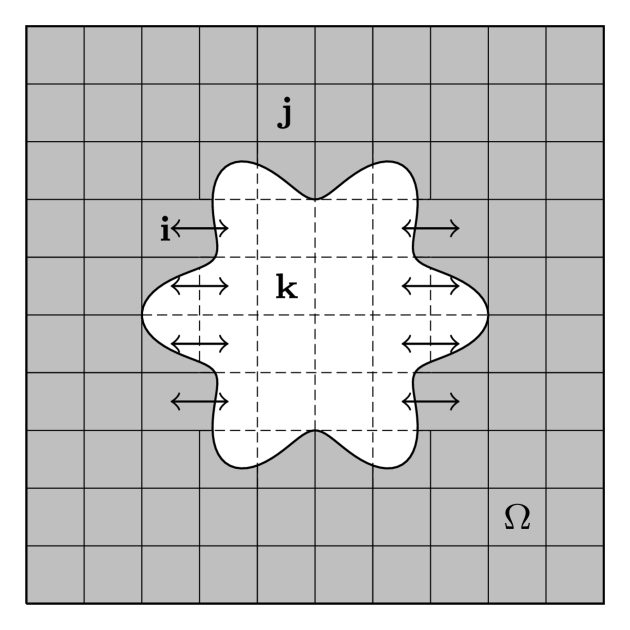
Figure 1: A Cartesian grid in the cut cell method. Here small cells with volume fraction below 0.3 have been merged. The cut cells $\mathbf{i}$, $\mathbf{j}$, and $\mathbf{k}$ are interface, pure and empty cells, respectively. The merged cut cells are linked by the symbol “$\leftrightarrow$”.

3.2 Finite volume approximation

Define the averaged $\phi$ over cell $\mathbf{i}$ by

(17) $$\left\langle\phi\right\rangle_{\mathbf{i}}:=\frac{1}{\lVert\mathcal{C}_{\mathbf{i}}\rVert}\int_{\mathcal{C}_{\mathbf{i}}}\phi(\mathbf{x})\ \mathrm{d}\mathbf{x},$$

the averaged $\phi$ over face $\mathbf{i}+\frac{1}{2}\bm{\mathrm{e}}^{d}$ by

(18) $$\left\langle\phi\right\rangle_{\mathbf{i}+\frac{1}{2}\bm{\mathrm{e}}^{d}}:=\frac{1}{\lVert\mathcal{F}_{\mathbf{i}+\frac{1}{2}\bm{\mathrm{e}}^{d}}\rVert}\int_{\mathcal{F}_{\mathbf{i}+\frac{1}{2}\bm{\mathrm{e}}^{d}}}\phi(\mathbf{x})\ \mathrm{d}\mathbf{x},$$

and averaged $\phi$ over cell boundary $\mathcal{S}_{\mathbf{i}}$ by

(19) $$\left\lAngle\phi\right\rAngle_{\mathbf{i}}:=\frac{1}{\|\mathcal{S}_{\mathbf{i}}\|}\int_{\mathcal{S}_{\mathbf{i}}}\phi(\mathbf{x})\ \mathrm{d}\mathbf{x}.$$

On cut cells sufficiently far from irregular boundaries, a routine Taylor expansion justifies the following fourth-order difference formulas for the discrete gradient and discrete Laplacian:

(20) $$\left\langle\frac{\partial\phi}{\partial x_{d}}\right\rangle_{\mathbf{i}} =\frac{1}{12h}\Big{(}-\left\langle\phi\right\rangle_{\mathbf{i}+2\bm{\mathrm{e}}^{d}}+8\left\langle\phi\right\rangle_{\mathbf{i}+\bm{\mathrm{e}}^{d}}-8\left\langle\phi\right\rangle_{\mathbf{i}-\bm{\mathrm{e}}^{d}}+\left\langle\phi\right\rangle_{\mathbf{i}-2\bm{\mathrm{e}}^{d}}\Big{)}+\operatorname{O}(h^{4}),$$

(21) $$\left\langle\Delta\phi\right\rangle_{\mathbf{i}} =\frac{1}{12h^{2}}\sum_{d}\Big{(}-\left\langle\phi\right\rangle_{\mathbf{i}+2\bm{\mathrm{e}}^{d}}+16\left\langle\phi\right\rangle_{\mathbf{i}+\bm{\mathrm{e}}^{d}}-30\left\langle\phi\right\rangle_{\mathbf{i}}+16\left\langle\phi\right\rangle_{\mathbf{i}-\bm{\mathrm{e}}^{d}}+\left\langle\phi\right\rangle_{\mathbf{i}-2\bm{\mathrm{e}}^{d}}\Big{)}+\operatorname{O}(h^{4}).$$

For the cross derivative $\frac{\partial^{2}\phi}{\partial x_{i}\partial x_{j}}(i\neq j)$, a fourth-order discretization is obtained from the iterated applications of (20) in the $i$th and $j$th directions. The stencils of the Laplacian operator and the cross operator are thus

(22) $$\mathcal{S}_{\mathrm{Lap}}(\mathbf{i})=\{\mathbf{i}+m\bm{\mathrm{e}}^{d}:m=0,\pm 1,\pm 2,d=1,2.\},$$

and

(23) $$\mathcal{S}_{\mathrm{Cro}}(\mathbf{i})=\{\mathbf{i}+m_{1}\bm{\mathrm{e}}^{1}+m_{2}\bm{\mathrm{e}}^{2}:m_{1},m_{2}=\pm 1,\pm 2.\}.$$

A cell $\mathbf{i}$ will be called a regular cell if each cell $\mathbf{j}\in\mathcal{S}_{\mathrm{Lap}}(\mathbf{i})\cup\mathcal{S}_{\mathrm{Cro}}(\mathbf{i})$ is a pure cell. A non-empty cell is either regular or irregular. The region covered by regular and irregular cells are called the regular region and the irregular region, respectively. For a regular cell $\mathbf{i}$, the elliptic operator can be evaluated using Equations (20) and (21). For an irregular cell $\mathbf{i}$, the elliptic operator can be evaluated by first generating poised lattices near $\mathcal{C}_{\mathbf{i}}$ (Section 2.2), then locally reconstructing a multivariate polynomial (Section 2.3 and 3.3), and finally evaluating the multi-dimensional quadratures (Section 2.4).

3.3 Discretization of the spatial operators

In this section, we consider the discretization of a linear differential operator $\mathcal{L}$ of order $q$ near the irregular domain boundary. Although we are mainly concerned with the second-order elliptic operator

(24) $$u\mapsto a\frac{\partial^{2}u}{\partial x_{1}^{2}}+b\frac{\partial^{2}u}{\partial x_{1}\partial x_{2}}+c\frac{\partial^{2}u}{\partial x_{2}^{2}},$$

the methodology applies to other linear operators as well. Denote by $\mathcal{N}$ the operator of the boundary condition: for example, $\mathcal{N}=\mathbf{I}_{\text{d}}$ for the Dirichlet condition, $\mathcal{N}=\partial/\partial\mathbf{n}$ for the Neumann condition, and $\mathcal{N}=\gamma_{1}+\gamma_{2}\cdot\partial/\partial\mathbf{n}~(\gamma_{1},\gamma_{2}\in\mathbb{R})$ for the Robin condition. Hereafter we fix $\mathbf{i}\in\mathbb{Z}^{\scriptsize\textsf{D}}$ and let

(25) $$\mathcal{X}=\mathcal{X}(\mathbf{i})=\mathcal{S}_{\mathrm{PLG}}(\mathbf{i})\cup\left\{\mathcal{S}_{\mathbf{i}}\right\}$$

be the stencil for discretizing $\mathcal{L}$ on $\mathcal{C}_{\mathbf{i}}$, where $\mathcal{S}_{\mathrm{PLG}}(\mathbf{i})=\left\{\mathcal{C}_{\mathbf{j}_{1}},\mathcal{C}_{\mathbf{j}_{2}},\cdots,\mathcal{C}_{\mathbf{j}_{N}}\right\}$ is the poised lattices generated by PLG algorithm with $N=\dim{\Pi_{n}^{\scriptsize\textsf{D}}}$; see Figure 2 for an example. Traditional methods usually select larger stencil or keep adding nearby cells to ensure the solvability of the linear system. But blindly expanding the stencil may lead to a large number of redundant points, deteriorating computational efficiency. This is precisely an advantage of our PLG algorithm.

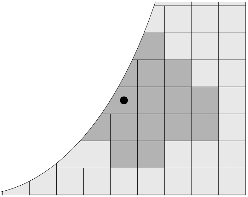
Figure 2: An example of poised lattices covered by dark-shaded cells in finite-volume discretization for ${\scriptsize\textsf{D}}=2$ and $n=4$. The cell $\mathcal{C}_{\mathbf{i}}$ is marked by a bullet $\bullet$.

We have assumed that $\mathcal{X}$ contains the boundary face $\mathcal{S}_{\mathbf{i}}$ and the treatment of the other case is similar. In the following, we reserve the symbol $n$ for the degree of polynomial fitting (and of the lattice $\mathcal{X}$, of course), the index $k\ (1\leq k\leq N)$ for the interpolation sites, and the index $j\ (1\leq j\leq N)$ for the basis of $\Pi_{n}^{\scriptsize\textsf{D}}$. Given the cell averages and the boundary data

(26) $$\hat{u} =\left[u_{1},\cdots,u_{N},u_{\mathrm{b}}\right]^{T}$$

$$=\left[\left\langle u\right\rangle_{\mathbf{j}_{1}},\cdots,\left\langle u\right\rangle_{\mathbf{j}_{N}},\left\lAngle\mathcal{N}u\right\rAngle_{\mathbf{i}}\right]^{T}\in\mathbb{R}^{N+1},$$

the goal is to determine the coefficients

(27) $$\hat{\beta}=\left[\beta_{1},\cdots,\beta_{N},\beta_{\mathrm{b}}\right]^{T}\in\mathbb{R}^{N+1},$$

such that the linear approximation formula

(28) $$\left\langle\mathcal{L}u\right\rangle_{\mathbf{i}} =\sum_{k=1}^{N}\beta_{k}u_{k}+\beta_{\mathrm{b}}u_{\mathrm{b}}+\operatorname{O}(h^{n-q+1})$$

$$=\hat{\beta}^{T}\hat{u}+\operatorname{O}(h^{n-q+1})$$

holds for all sufficiently smooth function $u:\mathbb{R}^{\scriptsize\textsf{D}}\rightarrow\mathbb{R}$.

We establish the equations on $\hat{\beta}$ by requiring that (28) holds exactly for all $u\in\Pi_{n}^{\scriptsize\textsf{D}}$, i.e.

(29) $$\left\langle\mathcal{L}u\right\rangle_{\mathbf{i}}=\sum_{k=1}^{N}\beta_{k}u_{k}+\beta_{\mathrm{b}}u_{\mathrm{b}}$$

for all $u\in\Pi_{n}^{\scriptsize\textsf{D}}$. Since $\left\{\phi_{j}\right\}_{j=1}^{N}$ is a basis of $\Pi_{n}^{\scriptsize\textsf{D}}$, it is equivalent to say

(30) $$\left\langle\mathcal{L}\phi_{j}\right\rangle_{\mathbf{i}}=\sum_{k=1}^{N}\beta_{k}\left\langle\phi_{j}\right\rangle_{\mathbf{j}_{k}}+\beta_{\mathrm{b}}\left\lAngle\phi_{j}\right\rAngle_{\mathbf{i}}$$

for $j=1,\cdots,N$, or simply

(31) $$M\hat{\beta}=\hat{L},$$

where

(32) $$M =\begin{bmatrix}\left\langle\phi_{1}\right\rangle_{\mathbf{j}_{1}}&\left\langle\phi_{1}\right\rangle_{\mathbf{j}_{2}}&\cdots&\left\langle\phi_{1}\right\rangle_{\mathbf{j}_{N}}&\left\lAngle\mathcal{N}\phi_{1}\right\rAngle_{\mathbf{i}}\\ \left\langle\phi_{2}\right\rangle_{\mathbf{j}_{1}}&\left\langle\phi_{2}\right\rangle_{\mathbf{j}_{2}}&\cdots&\left\langle\phi_{2}\right\rangle_{\mathbf{j}_{N}}&\left\lAngle\mathcal{N}\phi_{2}\right\rAngle_{\mathbf{i}}\\ \vdots&\vdots&\ddots&\vdots&\vdots\\ \left\langle\phi_{N}\right\rangle_{\mathbf{j}_{1}}&\left\langle\phi_{N}\right\rangle_{\mathbf{j}_{2}}&\cdots&\left\langle\phi_{N}\right\rangle_{\mathbf{j}_{N}}&\left\lAngle\mathcal{N}\phi_{N}\right\rAngle_{\mathbf{i}}\\ \end{bmatrix}\in\mathbb{R}^{N\times(N+1)},$$

and

(33) $$\hat{L} =\begin{bmatrix}\left\langle\mathcal{L}\phi_{1}\right\rangle_{\mathbf{i}}&\left\langle\mathcal{L}\phi_{2}\right\rangle_{\mathbf{i}}&\cdots&\left\langle\mathcal{L}\phi_{N}\right\rangle_{\mathbf{i}}\end{bmatrix}^{T}\in\mathbb{R}^{N}.$$

This is an underdetermined system on $\hat{\beta}$ and we seek the weighted minimum norm solution via

(34) $$\min_{\beta\in\mathbb{R}^{N+1}}\left\|\beta\right\|_{W^{-1}}\quad\mathrm{s.t.}\quad M\beta=\hat{L}.$$

Since $M$ has full row rank, it follows from Proposition 2.8 that

(35) $$\hat{\beta}=WM^{T}\left(MWM^{T}\right)^{-1}\hat{L}.$$

The weight matrix $W$ is used to penalize large coefficients on the cells far from $\mathcal{C}_{\mathbf{i}}$. For simplicity, we set $W^{-1}=\operatorname{diag}\left(w_{1},\cdots,w_{N},w_{\mathrm{b}}\right)$, where

(36a) $$w_{k} =\max\left\{\|\mathbf{j}_{k}-\mathbf{i}\|_{2},w_{\mathrm{min}}\right\},$$

(36b) $$w_{\mathrm{b}} =w_{\mathrm{min}},$$

and $w_{\mathrm{min}}$ is set to $1/2$ to avoid zero weights.

In practice, to maintain a good conditioning, we use the following basis (with recentering and scaling)

(37) $$\Phi_{n}^{D}(h;\mathbf{p})=\left\{\left(\frac{\mathbf{x}-\mathbf{p}}{h}\right)^{\bm{\alpha}}:0\leq|\bm{\alpha}|\leq n\right\},$$

where $\mathbf{p}\in\mathbb{R}^{D}$ is the center (or simply the center of the bounding box) of the interpolation sites.

3.4 Discrete elliptic problems

In this section, we discuss the fourth-order discretization of the constant-coefficient elliptic equation (1) with the boundary condition

(38) $$\mathbf{n}\cdot\nabla u=g\quad\text{on }\partial\Omega.$$

For ease of exposition, we specify the Neumann condition but the treatment of the other cases is similar. Define $\hat{u}$ to be the vector consisting of the cell averages of the unknown function $u$, and define $\hat{f}$ accordingly. Define $\hat{g}$ to be the vector consisting of the boundary-face averages of the boundary condition $g$. Combining the fourth-order difference formula (21) and the third-order finite-volume PLG approximation (28), we obtain the discretization

(39) $$L_{0}\left(\hat{u},\hat{g}\right)=\hat{f}.$$

Note that the linearity of $L_{0}(\cdot,\cdot)$ in each variable is implied by our construction; hence we can rewrite (39) into

(40) $$L\hat{u}+N\hat{g}=\hat{f},$$

where $L$ and $N$ are both matrices. Next we transform (40) into the residual form

(41) $$L\hat{u}=\hat{r}\coloneqq\hat{f}-N\hat{g},$$

and further split it into two row blocks, i.e.

(42) $$\begin{bmatrix}L_{11}&L_{12}\\ L_{21}&L_{22}\end{bmatrix}\begin{bmatrix}\hat{u}_{1}\\ \hat{u}_{2}\end{bmatrix}=\begin{bmatrix}\hat{r}_{1}\\ \hat{r}_{2}\end{bmatrix}.$$

The split $\hat{u}=\left[\hat{u}_{1}^{T}\ \hat{u}_{2}^{T}\right]^{T}$ is based on the discretization type: if the cell $\mathbf{i}$ is a regular cell, then the cell average $\left\langle u\right\rangle_{\mathbf{i}}$ is contained in $\hat{u}_{1}$; otherwise it is contained in $\hat{u}_{2}$. Consequently, the sub-block $L_{11}$ has a regular structure whereas the structures of the other sub-blocks are only known to be sparse.

4 Multigrid algorithm

In this section, we present the multigrid algorithm for solving the discrete elliptic equation (42). The overall procedure is geometric-based. First we initialize a hierarchy of successively coarsened grids

(43) $$\Omega^{\ast}=\left\{\Omega^{(m)}:0\leq m\leq M\right\},$$

where $\Omega^{(m)}$ is obtained by embedding $\Omega$ into a rectangular grid of step size $h^{(m)}=2^{m}h^{(0)}$. On each level we construct the discrete elliptic operator $L^{(m)}$ via the finite-volume PLG discretization discussed in the last section. We stop at some $\Omega^{(M)}$ where the direct solution (say, via LU factorization) of the discrete linear system is inexpensive.

We should mention that the finite-volume PLG discretization prohibits the direct application of the traditional geometric multigrid method. This is because: (1) The Gauss-Siedel and the (weighted) Jacobi iteration are not guaranteed to converge due to the presence of the irregular sub-blocks $L_{12},L_{21}$ and $L_{22}$ in (42); (2) Simple grid-transfer operators, such as the volume-weighted restriction and the linear interpolation cannot be applied near the irregular boundary. In the following, we adhere to the multigrid framework [4] but propose modifications to the V-cycle (Algorithm 2) components so that the algorithm is still effective with high-order scheme and arbitrarily complex irregular boundaries. To improve V-cycles, the full multigrid (FMG) cycle, which utilizes the multigrid concept to build an accurate initial guess, is also implemented; see Figure 3. Although FMG cycles are more expensive than V-cycles, it has been widely used because of the better initial guesses and the optimal complexity [4].

Algorithm 2 VCycle$(L^{(m)},\hat{u}^{(m)},\hat{r}^{(m)},\nu_{1},\nu_{2})$

1:An integer $m$ indicating the level, with 0 being the finest;

2:the discrete elliptic operator $L^{(m)}$ on the $m$th level;

3:the initial guess $\hat{u}^{(m)}$;

4:the residual $\hat{r}^{(m)}$ on the $m$th level;

5:the smooth parameters $\nu_{1},\nu_{2}$.

6:The solution to the algebraic equation $L^{(m)}\hat{u}^{(m)}=\hat{r}^{(m)}$.

7:if $m=M$ then

8:  Solve $L^{(M)}\hat{u}^{(M)}=\hat{r}^{(M)}$ using the bottom solver.

9:else

10:  Apply the smoother to $L^{(m)}\hat{u}^{(m)}=\hat{r}^{(m)}$ for $\nu_{1}$ times.

11:  Compute the coarse residual by restriction:

12: $\hat{r}^{(m+1)}=\text{{Restrict}}(\hat{r}^{(m)}-L^{(m)}\hat{u}^{(m)}).$

13:  Recursively solve the algebraic equation on the coarse grid:

14: $\hat{u}^{(m+1)}=\mathbf{0}$,

15: $\hat{u}^{(m+1)}=\text{{VCycle}}(L^{(m+1)},\hat{u}^{(m+1)},\hat{r}^{(m+1)},\nu_{1},\nu_{2})$.

16:  Prolong the correction and update the solution:

17: $\hat{u}^{(m)}=\hat{u}^{(m)}+\text{{Prolong}}(\hat{u}^{(m+1)})$.

18:  Apply the smoother to $L^{(m)}\hat{u}^{(m)}=\hat{r}^{(m)}$ for $\nu_{2}$ times.

19:end if

20:return $\hat{u}^{(m)}$.

Figure 3: Illustration of the FMG cycle for a grid with four levels. FMG begins with a descent to the coarsest grid $\Omega^{8h}$; this is represented by the downward dashed line segments. Then the solution is prolongated to $\Omega^{4h}$ and used as the initial guess to the V-cycle on $\Omega^{4h}$. This “prolongation $+$ V-cycle” process is repeated recursively: the prolongation is represented by an upward dashed line and the V-cycles are represented by the solid lines.

4.1 Multigrid components

First we discuss the smoother used in Algorithm 2. To avoid cluttering, we temporarily omit the superscript ^(m) indicating the grid level, and use the prime variables to denote the quantities after one iteration of the smoother. Then, to ensure convergence, we have made the following adjustments.

1. The $\omega$-weighted Jacobi iteration

   (44) $$\hat{u}^{\prime}_{1}=D^{-1}\left[(1-\omega)D+\omega O\right]\hat{u}_{1}+\omega D^{-1}O\left(\hat{r}_{1}-L_{12}\hat{u}_{2}\right)$$

   is applied in a pointwise fashion to $\hat{u}_{1}$, where $D$ is the diagonal part of $L_{11}$ and $O=D-L_{11}$ is the off-diagonal part;

2. A block update

   (45) $$L_{22}\hat{u}^{\prime}_{2}=\hat{r}_{2}-L_{21}\hat{u}^{\prime}_{1}$$

   is applied to obtain $\hat{u}^{\prime}_{2}$.

Several comments are in order. First, it is favorable to pre-compute the LU factorization of the sub-block $L_{22}$, allowing for solving the linear system (45) with multiple right-hand-sides with minimal cost. Second, we have used the updated value $\hat{u}_{1}^{\prime}$ instead of $\hat{u}_{1}$ in (45). Hence, the overall iteration is more like Gauss-Siedel in a blockwise fashion. After two iterations of the smoother, we have

(46a) $$\hat{e}^{\prime}_{1} =D^{-1}\left[(1-\omega)D+\omega O\right]\hat{e}_{1},$$

(46b) $$\hat{e}^{\prime}_{2} =\mathbf{0},$$

where $\hat{e}=[\hat{e}_{1}^{T}~\hat{e}_{2}^{T}]^{T}$ and its prime version are the solution errors in (42) before and after the iteration, respectively. From (46a) we see that the error on the interior cells is essentially damped by an $\omega$-weighted Jacobi iteration, exactly what we would expect from an effective smoother.

By virtue of (46b), not only the error but also the residual corresponding to the $\hat{u}_{2}$ part are identically zero after two or more iterations of the smoother. Consequently, grid-transfer operators that carefully handles the irregular cells near the domain boundary are not mandatory. In practice, we apply the volume weighted restriction

(47) $$\left\langle u\right\rangle^{(m+1)}_{\lfloor\mathbf{i}/2\rfloor}=2^{-{\scriptsize\textsf{D}}}\sum_{\mathbf{j}\in\left\{0,1\right\}^{\scriptsize\textsf{D}}}\left\langle u\right\rangle^{(m)}_{\mathbf{i}+\mathbf{j}}$$

and the patchwise-constant interpolation

(48) $$\left\langle u\right\rangle^{(m)}_{\mathbf{i}}=\left\langle u\right\rangle^{(m+1)}_{\lfloor\mathbf{i}/2\rfloor}$$

for regular cells, while leaving the correction and the residual for partial cells to zero.

On the coarsest level we invoke the LU solver on $L^{(M)}\hat{u}^{(M)}=\hat{r}^{(M)}$ where the LU factorization of $L^{(M)}$ is computed beforehand.

4.2 Optimal complexity of LU factorization for $L_{22}$

Since we frequently need to solve the linear system (45), it is essential to find efficient methods. Traditional LU factorization has a complexity of $\operatorname{O}(N^{3})$, where $N$ is the number of unknowns. In this section, we present an optimal LU factorization for $L_{22}$ achieved by reordering the unknowns, which has a complexity of only $\operatorname{O}(N)$. To be specific, let $\mathcal{I}_{\mathrm{bdry}}$ be the collection of all interface cells, i.e.

$$\mathcal{I}_{\mathrm{bdry}}\coloneqq\left\{\mathbf{i}\in\mathbb{Z}^{2}:\mathcal{C}_{\mathbf{i}}\neq\emptyset,\mathrm{C}_{\mathbf{i}}\right\}.$$

Let $\gamma:[0,1]\to\mathbb{R}^{2}$ be a parameterization of the Jordan curve $\partial\Omega$ with $\gamma(0)=\gamma(1)$. For each $\mathbf{i}\in\mathcal{I}_{\mathrm{bdry}}$, define $s(\mathbf{i})\in[0,1)$ such that

(49) $$\mathrm{dist}(\partial\Omega,R_{\mathbf{i}})=\|R_{\mathbf{i}}-\gamma(s(\mathbf{i}))\|,$$

where $R_{\mathbf{i}}$ is the cell center of $\mathbf{C}_{\mathbf{i}}$. Next we define the linear order $``\leq"$ on $\mathcal{I}_{\mathrm{bdry}}$ by requiring

(50) $$\mathbf{i}\leq\mathbf{j}\quad\mathrm{iff}\quad s(\mathbf{i})\leq s(\mathbf{j}).$$

We compute the ordering for the irregular cells according to Algorithm 3; see Figure 4 for an illustration. To measure the effectiveness of this ordering, we consider a decomposition of the reordered matrix $L_{22}$,

(51) $$L_{22}=L_{22,c}+\begin{bmatrix}O&L_{22,u}\\ O&O\end{bmatrix}+\begin{bmatrix}O&O\\ L_{22,l}&O\end{bmatrix},$$

where $L_{22,c}$ is a banded matrix, and $L_{22,u},L_{22,l}$ are square sub-matrices with small dimensions. The cyclic bandwidth of $L_{22}$, defined as the number $\lambda(L_{22,c},L_{22,u},L_{22,l})$, which is the maximum of the bandwidth of $L_{22,c}$ and the dimensions of $L_{22,u}$ and $L_{22,l}$, is associated with each decomposition in the form of (51). In practical numerical examples, the cyclic bandwidth of $L_{22}$ is found to be independent of the grid size and is no larger than $20$, even for very complex geometries. Consequently, the complexity of the LU factorization of the matrix $L_{22}$ can be kept linear with its dimension (see Section 5.2), provided no pivoting is performed. For details on the LU factorization of the banded matrix, see [9].

Algorithm 3 An order over the irregular cells.

1: The collection of all interface cells $\mathcal{I}_{\mathrm{bdry}}$ ordered by $``\leq"$ defined in (50).

2: An order over the irregular cells, represented by a non-negative integer $P(\mathbf{i})$ for each irregular cell $\mathbf{i}$.

3:Initialize $P(\mathbf{i})=-1$ for each irregular cell $\mathbf{i}$

4:$k\leftarrow 0$

5:for $\mathbf{i}\in(\mathcal{I}_{\mathrm{bdry}},\leq)$ do

6:  for  all $\mathbf{j}\in\mathbb{Z}^{2}$ with $\left\|\mathbf{i}-\mathbf{j}\right\|_{\infty}\leq 2$ do

7:   if  cell $\mathbf{j}$ is irregular $\mathrm{and}$ $P(\mathbf{j})=-1$ then

8:     $P(\mathbf{j})=k$

9:     $k\leftarrow k+1$

10:   end if

11:  end for

12:end for

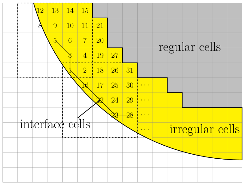
Figure 4: An illustration for the linear order output by Algorithm 3. The regular cells are shaded light gray, while the irregular cells are shaded yellow.

4.3 Complexity

Let $h=h^{(0)}$ be the step size of the finest grid. We assume the sub-vector $\hat{u}_{1}$ in (42) has dimension $\operatorname{O}(h^{-2})$ and the sub-vector $\hat{u}_{2}$ has dimension $\operatorname{O}(h^{-1})$.

1. Setup. Consider the setup time on the finest level. During the construction of the discrete Laplacian and cross operators, the finite-volume PLG discretization is invoked to obtain the $\left[L_{21}\ L_{22}\right]$ blocks. This requires $\operatorname{O}(h^{-1})$ time since the PLG discretization is $\operatorname{O}(1)$ for each cell and these blocks are sparse with $\operatorname{O}(h^{-1})$ rows. We then compute the sparse LU factorization of $L_{22}$, which takes $\operatorname{O}(h^{-1})$ time thanks to its sparsity and small bandwidth; see also the numerical evidences in Section 5.2. For the complete hierarchy of grids, the complexity is bounded by a constant multiple of that on the finest level, so the total setup time is $\operatorname{O}(h^{-1})$.

2. Solution. We first bound the complexity of a single V-cycle (Algorithm 2) and a single FMG cycle (Figure 3). The bottom solver requires $\operatorname{O}(1)$ time since it operates on the coarsest level only. On the finest level, the pointwise Jacobi iteration on $\hat{u}_{1}$  44 requires $\operatorname{O}(h^{-2})$ time. The blockwise update on $\hat{u}_{2}$ 45 requires $\operatorname{O}(h^{-1})$ time, provided the LU factorization of $L_{22}$ is available. Each of the restriction and the prolongation requires $\operatorname{O}(h^{-2})$. Since the complexity of the complete hierarchy is bounded by a constant multiple of that on the finest level, we know that both a single V-cycle and a single FMG cycle have a complexity of $\operatorname{O}(h^{-2})$.

   To bound the complexity of the overall solution procedure, we still need to estimate the number of V-cycles and FMG cycles needed to reduce the initial residual to a given fraction. Considering the recursive nature of V-cycle and the smoothing property (46), we expect that error modes of all frequency can be effectively damped by the multigrid algorithm, similar to their behavior on rectangular domains, with V-cycles having a convergence factor $\gamma$ that is independent of $h$. Since V-cycles must reduce the algebraic error from $\operatorname{O}(1)$ to $\operatorname{O}(h^{4})$, the number $\mu$ of V-cycles required must satisfy $\gamma^{\mu}=\operatorname{O}(h^{4})$ or $\mu=\operatorname{O}(h^{-1})$. Because the cost of a single V-cycle is $\operatorname{O}(h^{-2})$, the cost of V-cycles is $\operatorname{O}(h^{-2}\log(h^{-1}))$. The FMG cycle costs a little more per cycle than the V-cycle. However, a properly designed FMG cycle can be much more effective overall because it supplies a very good initial guess to the final V-cycles on the finest level. This result in only $\operatorname{O}(1)$ V-cycles are needed on the finest grid (see [3] for a more detailed discussion). This means that the total complexity of FMG cycles is $\operatorname{O}(h^{-2})$, which is optimal. This is also confirmed by numerical examples in Section 5.2.

We point out that the solution time of $\operatorname{O}(h^{-2})$ is the best possible bound we can achieve in irregular domains, since solving an elliptic equation in a rectangular grid with $\operatorname{O}(h^{-2})$ cells using the geometric multigrid method has exactly $\operatorname{O}(h^{-2})$ complexity. Detailed numerical results on the efficiency of the multigrid algorithm are reported in Section 5.2.

5 Numerical tests

In this section we demonstrate the accuracy and efficiency of our method by various test problems in irregular domains. Define the $L^{p}$ norms

(52) $$\|u\|_{p}=\left\{\begin{aligned} &\left(\frac{1}{\|\Omega\|}\sum\left\|\mathcal{C}_{\mathbf{i}}\right\|\cdot\left|\left\langle u\right\rangle_{\mathbf{i}}\right|^{p}\right)^{1/p}\quad&&p=1,2,\\ &\max\ \left|\left\langle u\right\rangle_{\mathbf{i}}\right|\quad&&p=\infty,\end{aligned}\right.$$

where the summation and the maximum are taken over the non-empty cells in the computational domain.

5.1 Convergence tests

Problem 1. Consider a problem [11, Problem 3] of Poisson’s equation on the irregular domain $\Omega=R\cap\Omega_{1}$, where $R$ is the unit box centered at the origin and

(53) $$\Omega_{1}=\left\{\left(r,\theta\right):r\geq 0.25+0.05\cos 6\theta\right\}.$$

Here $\left(r,\theta\right)$ are the polar coordinates satisfying $(x_{1},x_{2})=(r\cos\theta,r\sin\theta)$. A Dirichlet condition is imposed on the rectilinear sides $\partial R$ while a Neumann condition is imposed on the irregular boundary $\partial\Omega_{1}$. Both the right-hand-side and the boundary conditions are derived from the exact solution

(54) $$u(r,\theta)=r^{4}\cos 3\theta.$$

The numerical solution and the solution error on the grid of $h=1/80$ are shown in Figure 5(a) and 5(b), respectively. The error appears oscillating near the irregular boundary due to the rapidly varying truncation errors induced by the PLG discretization. However, it does not affect the fourth-order convergence of the numerical solution as confirmed by the grid-refinement tests.

The truncation errors and the solution errors are listed in Table 1 and 2. The convergence rates of the truncation errors are asymptotically close to 3, 4 and 3.5 in $L^{\infty}$ norm, $L^{1}$ norm and $L^{2}$ norm, respectively. This suggests that the PLG approximation is third-order accurate on the boundary cells of codimension one and fourth-order accurate on the interior cells. The convergence rates of the solution errors are close to 4 in all norms as expected. Also included in the tables are the comparisons with the second-order EB method by Johansen and Colella [11]. Our method is much more accurate than the second-order EB method in terms of solution errors. In particular, the $L^{\infty}$ norm of the error on the grid of $h=1/80$ in our method is smaller by a factor of 40 than that on the grid of $h=1/320$ in the EB method. On the grid of $h=1/320$, the $L^{\infty}$ norm of the error in our method is about $1/8000$ of that in the second-order EB method.

Truncation errors of the EB method by Johansen and Colella [11]
$h$	1/40	rate	1/80	rate	1/160	rate	1/320
$L^{\infty}$	1.66e$-$03	2.0	4.15e$-$04	2.0	1.04e$-$04	2.0	2.59e$-$05
Truncation errors of the current method
$h$	1/40	rate	1/80	rate	1/160	rate	1/320
$L^{\infty}$	2.94e-04	0.78	1.71e-04	2.83	2.41e-05	2.95	3.13e-06
$L^{1}$	1.03e-05	3.74	7.70e-07	4.16	4.30e-08	3.87	2.94e-09
$L^{2}$	3.30e-05	3.00	4.13e-06	3.65	3.29e-07	3.45	3.01e-08

Table 1: Truncation errors of Problem 1, with Dirichlet condition on the rectilinear sides and Neumann condition on the irregular boundary. Comparisons with a second-order EB method [11] are shown.

Solution errors of the EB method by Johansen and Colella [11]
$h$	1/40	rate	1/80	rate	1/160	rate	1/320
$L^{\infty}$	4.78e$-$05	1.85	1.33e$-$05	1.98	3.37e$-$06	1.95	8.72e$-$07
Solution errors of the current method
$h$	1/40	rate	1/80	rate	1/160	rate	1/320
$L^{\infty}$	3.68e-07	4.08	2.17e-08	3.70	1.67e-09	3.92	1.10e-10
$L^{1}$	3.77e-08	3.85	2.62e-09	4.41	1.23e-10	3.79	8.86e-12
$L^{2}$	6.24e-08	4.12	3.59e-09	4.19	1.97e-10	3.81	1.41e-11

Table 2: Solution errors of Problem 1, with Dirichlet condition on the rectilinear sides and Neumann condition on the irregular boundary. Comparisons with a second-order EB method [11] are shown.

(a) Numerical solution

(b) Solution error

Figure 5: Solving Problem 1 on the grid of $h=1/80$.

Problem 2. Consider a problem from [6, §5.1] where Poisson’s equation is solved on the domain $\Omega=R\cap\Omega_{2}$, $R$ is the unit box $[0,1]^{2}$ and $\Omega_{2}$ is the exterior of the ellipse defined by

(55) $$\sum_{i=1}^{2}\left(\frac{x_{i}-c_{i}}{a_{i}}\right)^{2}=1.$$

The parameters are $(c_{1},c_{2})=(1/2,1/2)$ and $(a_{1},a_{2})=(1/8,1/4)$. A Dirichlet condition is imposed on the rectilinear sides $\partial R$, and either a Dirichlet or a Neumann condition is imposed on the irregular boundary $\partial\Omega_{2}$. The right-hand-side and the boundary conditions are derived from the exact solution

(56) $$u=\Pi_{i=1}^{2}\sin(\pi x_{i}).$$

The solution errors with Neumann condition and Dirichlet condition on the grid of $h=1/256$ are shown in Figure 6(a) and 6(b), respectively. The errors of both cases appear smooth over the entire domain, and approach zero on the Dirichlet boundaries. In the Neumann case, the maximum of error appears on the ellipse boundary; while in the Dirichlet case, the maximum of error appears in the interior of the domain.

The solution errors are listed in Table 3 and 4. With either boundary condition, the solutions demonstrate a fourth-order convergence in all norms in the grid-refinement tests. Also included in the tables are the comparisons with a recently developed fourth-order EB method [6]. It is observed that the solution errors of our method are smaller than those in [6] in all norms. For example, on the grid of $h=1/512$, the solution error in our method is about one half of that in [6] in the case of Neumann condition, and about one third in the case of Dirichlet condition.

A fourth-order EB method by Devendran et al. [6]
$h$	1/64	rate	1/128	rate	1/256	rate	1/512
$L^{\infty}$	1.83e-07	3.96	1.18e-08	3.98	7.43e-10	3.88	5.05e-11
$L^{1}$	6.90e-08	3.95	4.46e-09	3.97	2.83e-10	3.86	1.94e-11
$L^{2}$	8.67e-08	3.96	5.56e-09	3.98	3.51e-10	3.87	2.40e-11
Current method
$h$	1/64	rate	1/128	rate	1/256	rate	1/512
$L^{\infty}$	9.17e-08	3.87	6.29e-09	3.87	4.31e-10	4.04	2.62e-11
$L^{1}$	1.99e-08	3.49	1.76e-09	3.67	1.38e-10	4.12	7.99e-12
$L^{2}$	2.66e-08	3.55	2.27e-09	3.72	1.73e-10	4.12	9.96e-12

Table 3: Solution errors of Problem 2, with Dirichlet condition on the rectilinear sides and Neumann condition on the irregular boundary. Comparisons with a fourth-order EB method [6] are shown.

A fourth-order EB method by Devendran et al. [6]
$h$	1/64	rate	1/128	rate	1/256	rate	1/512
$L^{\infty}$	4.15e-08	4.04	2.53e-09	4.01	1.56e-10	3.84	1.09e-11
$L^{1}$	1.91e-08	4.02	1.17e-09	3.99	7.37e-11	3.82	5.20e-11
$L^{2}$	2.30e-08	4.04	1.40e-09	4.01	8.72e-11	3.83	6.11e-12
Current method
$h$	1/64	rate	1/128	rate	1/256	rate	1/512
$L^{\infty}$	4.96e-08	5.79	8.95e-10	4.12	5.14e-11	3.94	3.35e-12
$L^{1}$	8.88e-09	4.34	4.39e-10	4.11	2.55e-11	4.16	1.42e-12
$L^{2}$	1.03e-08	4.35	5.06e-10	4.10	2.95e-11	4.13	1.68e-12

Table 4: Solution errors of Problem 2, with Dirichlet condition on the domain boundaries. Comparisons with a fourth-order EB method [6] are shown.

(a) Neumann condition on the irregular boundary.

(b) Dirichlet condition on the irregular boundary.

Figure 6: Solution errors of Problem 2 with $h=1/256$. The Dirichlet condition is applied on the rectilinear sides.

Problem 3.

Consider solving the constant-coefficient elliptic equation (1) with different combinations of $(a,b,c)$ and $\Omega$:

1. $\Omega$ is the unit box $[0,1]^{2}$ and $(a,b,c)=(1,0,2)$.

2. $\Omega$ is the unit box rotated counterclockwise by $\pi/6$. In this domain, a system equivalent to case (i) would have $\left(a,b,c\right)=\left(5/4,-\sqrt{3}/2,7/4\right)$.

For case (i), the regular geometry and the absence of cross-derivative terms permits the usage of one-dimensional FD formula. In contrast, for case (ii) we invoke the PLG discretization near the irregular boundary to approximate the elliptic operator (24) as a whole. For case (i), the exact solution is given by

(57) $$u(x_{1},x_{2})=\sin(4x_{1})\cos(3x_{2}).$$

For the other case, the exact solution is rotated accordingly. Both test cases assume Dirichlet boundary condition.

The solution errors of both test cases are listed in Table 5. The convergence rates in both cases are close to 4 in all norms, again confirming the accuracy of our method. A comparison between case (i) and case (ii) shows that the $L^{\infty}$ norm of the error on the grid of $h=1/512$ in the latter case is roughly four times larger than that in the former case.

Case (i)
$h$	1/64	rate	1/128	rate	1/256	rate	1/512
$L^{\infty}$	3.68e-08	4.00	2.30e-09	4.00	1.44e-10	3.98	9.10e-12
$L^{1}$	1.13e-08	4.01	7.00e-10	4.01	4.35e-11	3.90	2.91e-12
$L^{2}$	1.50e-08	4.01	9.32e-10	4.00	5.81e-11	3.96	3.73e-12
Case (ii)
$h$	1/64	rate	1/128	rate	1/256	rate	1/512
$L^{\infty}$	1.57e-07	4.16	8.75e-09	3.93	5.75e-10	3.95	3.71e-11
$L^{1}$	4.92e-08	4.08	2.92e-09	3.92	1.92e-10	3.91	1.28e-11
$L^{2}$	6.15e-08	4.07	3.67e-09	3.90	2.47e-10	3.91	1.64e-11

Table 5: Solution errors of Problem 3, with Dirichlet condition on the domain boundaries.

5.2 Efficiency

Here we show the reductions of relative residuals and relative errors during the solution of Problem 2, and compare with their counterparts on the rectangular domain $R$. For both tests we use the same exact solution and the same multigrid parameters. In Figure 7, the change of relative residual in the irregular domain $\Omega$ (in the rectangular domain $R$, respectively) is plotted against the number of FMG cycle iterations in solid lines (in dashed lines, respectively). In both domains, the relative residuals are reduced by a factor of 11.3 per iteration before their stagnation at the 9th iteration. The relative errors, also shown in Figure 7, are reduced by a similar factor to that of the relative residuals. They stop to descend at the 7th iteration, implying that the algebraic accuracy of the solutions is reached. To summarize, the multigrid algorithm on irregular domains behave very much the same as it does on rectangular domains.

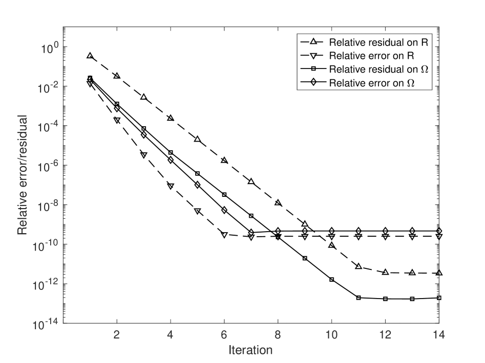
Figure 7: The reduction of relative residuals and relative errors during the solution of Problem 2 in the irregular domain $\Omega$ and in the rectangular domain $R$. The grid is $h=1/128$. The initial guess is the zero function. The multigrid parameters are $\omega=0.5$ and $\nu_{1}=\nu_{2}=3$. The ordinates are the relative residuals (relative errors) in $L^{\infty}$ norm, the abscissa is the number of FMG cycle iterations. The solid lines represent the results in the irregular domain and the dashed lines represent the results in the rectangular domain.

In Table 6 and 7, we report the time consumption of each component of the solver. The column “cut-cell generation” refers to the generation of cut cells and the cell merging process; see Section 3.1. The column “factorization of $L_{22}$” is self-evident. The column “poised lattice generation” comprises the execution of the PLG algorithm (Definition 2.6) over the irregular cells. The column “operator discretization” refers to the discretization procedure in Section 3.3, and finally the column “multigrid solution” refers solely to the time consumption of FMG cycles. It can be readiliy observed from the Tables that, the “cut-cell generation” and the “multigrid solution” grow quadratically with respect to the mesh size ($\sim h^{-2}$), while the other components only grow linearly ($\sim h^{-1}$). This confirms our anlysis in Section 4.3, and we conclude that the proposed multigrid algorithm is efficient in terms of solving elliptic equations in complex geometries.

$h$	cut-cell generation	factorization of $L_{22}$	poised lattice generation	operator discretization	multigrid solution
1/128	1.85e$-$03	6.59e$-$04	2.53e$-$03	1.45e$-$02	4.03e$-$02
1/256	6.31e$-$03	1.36e$-$03	5.17e$-$03	2.49e$-$02	8.20e$-$02
1/512	4.43e$-$02	2.67e$-$03	1.14e$-$02	4.58e$-$02	2.57e$-$01
1/1024	1.87e$-$01	5.30e$-$03	2.70e$-$02	9.01e$-$02	1.03e$-$00

Table 6: Time consumption (in seconds) of solving Problem 2 on an AMD Threadripper PRO 3975WX at 4.0Ghz with DDR4 2133MHz memory. The sparse factorization of the $L_{22}$ sub-block is computed by Eigen::SparseLU.

$h$	cut-cell generation	factorization of $L_{22}$	poised lattice generation	operator discretization	multigrid solution
1/128	6.27e$-$03	2.01e$-$03	9.18e$-$03	2.16e$-$01	9.23e$-$02
1/256	2.74e$-$02	3.59e$-$03	1.90e$-$02	4.36e$-$01	2.77e$-$01
1/512	1.06e$-$01	8.01e$-$03	4.09e$-$02	8.75e$-$01	9.60e$-$01
1/1024	4.05e$-$01	1.91e$-$02	9.21e$-$02	1.75e$+$00	3.71e$+$00

Table 7: Time consumption (in seconds) of solving Problem 3.

6 Conclusions

We have proposed a fast fourth-order cut cell method for solving constant-coefficient elliptic equations in two-dimensional irregular domains. For spatial discretization, we employ the PLG algorithm to generate finite-volume interpolation stencils near the irregular boundary. We then derive the high-order approximation to the elliptic operators from weighted least squares fitting. We design a multigrid algorithm for solving the resulting linear system with optimal complexity. We demonstrate the accuracy and efficiency of our method by various numerical tests.

Prospects for future research are as follows. We expect a straightforward extension of this work should yield a sixth- and higher-order solver for variable-coefficient elliptic equations. We also plan to develop a fourth-order INSE solver in irregular domains based on the GePUP formulation [30], where the pressure-Poisson equation (PPE) and the Helmholtz equations will be solved by the proposed elliptic solver.

References

- [1] A. S. Almgren, J. B. Bell, P. Colella, and T. Marthaler, A Cartesian grid projection method for the incompressible euler equations in complex geometries, SIAM J. Sci. Comput., 18 (1994), pp. 1289–1309.
- [2] M. J. Berger and R. J. LeVeque, A rotated difference scheme for Cartesian grids in complex geometries, AIAA, (1991), pp. 1–9.
- [3] A. Brandt and O. E. Livne, Multigrid Techniques, Society for Industrial and Applied Mathematics, 2011.
- [4] W. L. Briggs, V. E. Henson, and S. F. McCormick, A Multigrid Tutorial, Second Edition, Society for Industrial and Applied Mathematics, second ed., 2000.
- [5] D. L. Brown, R. Cortez, and M. L. Minion, Accurate projection methods for the incompressible Navier–Stokes equations, J. Comput. Phys., 168 (2001), pp. 464 – 499.
- [6] D. Devendran, D. Graves, H. Johansen, and T. Ligocki, A fourth-order Cartesian grid embedded boundary method for Poisson’s equation, Commun. Appl. Math. Comput. Sci., 12 (2017), pp. 51 – 79.
- [7] F. Gibou, R. P. Fedkiw, L.-T. Cheng, and M. Kang, A second-order-accurate symmetric discretization of the Poisson equation on irregular domains, J. Comput. Phys., 176 (2002), pp. 205 – 227.
- [8] S. Givant and P. Halmos, Introduction to Boolean Algebras, Springer-Verlag New York, 2009.
- [9] G. H. Golub and C. F. Van Loan, Matrix Computations, The Johns Hopkins University Press, fourth ed., 2013.
- [10] H. Ji, F.-S. Lien, and E. Yee, Numerical simulation of detonation using an adaptive Cartesian cut-cell method combined with a cell-merging technique, Comput. Fluids, 39 (2010), pp. 1041–1057.
- [11] H. Johansen and P. Colella, A Cartesian grid embedded boundary method for Poisson’s equation on irregular domains, J. Comput. Phys., 147 (1998), pp. 60 – 85.
- [12] H. Johnston and J.-G. Liu, Accurate, stable and efficient Navier–Stokes solvers based on explicit treatment of the pressure term, J. Comput. Phys., 199 (2004), pp. 221 – 259.
- [13] M. Kirkpatrick, S. Armfield, and J. Kent, A representation of curved boundaries for the solution of the Navier–Stokes equations on a staggered three-dimensional Cartesian grid, J. Comput. Phys., 184 (2003), pp. 1 – 36.
- [14] R. J. LeVeque and Z. Li, The immersed interface method for elliptic equations with discontinuous coefficients and singular sources, SIAM J. Numer. Anal., 31 (1994), pp. 1019–1044.
- [15] Z. Li, A fast iterative algorithm for elliptic interface problems, SIAM J. Numer. Anal., 35 (1998), pp. 230–254.
- [16] Z. Li and C. Wang, A fast finite differenc method for solving Navier-Stokes equations on irregular domains, Commun. Math. Sci., 1 (2003), pp. 180–196.
- [17] M. N. Linnick and H. F. Fasel, A high-order immersed interface method for simulating unsteady incompressible flows on irregular domains, J. Comput. Phys., 204 (2005), pp. 157 – 192.
- [18] J.-G. Liu, J. Liu, and R. L. Pego, Stability and convergence of efficient Navier-Stokes solvers via a commutator estimate, Commun. Pure Appl. Math., 60 (2007), pp. 1443–1487.
- [19] T. Liu, B. Khoo, and K. Yeo, Ghost fluid method for strong shock impacting on material interface, J. Comput. Phys., 190 (2003), pp. 651–681.
- [20] X.-D. Liu, R. P. Fedkiw, and M. Kang, A boundary condition capturing method for Poisson’s equation on irregular domains, J. Comput. Phys., 160 (2000), pp. 151 – 178.
- [21] X.-D. Liu, S. Osher, and T. Chan, Weighted essentially non-oscillatory schemes, J. Comput. Phys., 115 (1994), pp. 200–212.
- [22] P. McCorquodale, P. Colella, and H. Johansen, A Cartesian grid embedded boundary method for the heat equation on irregular domains, J. Comput. Phys., 173 (2001), pp. 620 – 635.
- [23] Y. Morinishi, T. Lund, O. Vasilyev, and P. Moin, Fully conservative higher order finite difference schemes for incompressible flow, J. Comput. Phys., 143 (1998), pp. 90 – 124.
- [24] P. Schwartz, M. Barad, P. Colella, and T. Ligocki, A Cartesian grid embedded boundary method for the heat equation and Poisson’s equation in three dimensions, J. Comput. Phys., 211 (2006), pp. 531 – 550.
- [25] C.-W. Shu and S. Osher, Efficient implementation of essentially non-oscillatory shock-capturing schemes, J. Comput. Phys., 77 (1988), pp. 439–471.
- [26] A. Sommariva and M. Vianello, Gauss–Green cubature and moment computation over arbitrary geometries, J. Comput. Appl. Math., 231 (2009), pp. 886 – 896.
- [27] D. Trebotich and D. T. Graves, An adaptive finite volume method for the incompressible Navier–Stokes equations in complex geometries, Commun. Appl. Math. Comput. Sci., 10 (2015), pp. 43–82.
- [28] L. Xu and T. Liu, Ghost-fluid-based sharp interface methods for multi-material dynamics: A review, Commun. Comput. Phys., 34 (2023), pp. 563–612.
- [29] Q. Zhang, A fourth-order approximate projection method for the incompressible Navier–Stokes equations on locally-refined periodic domains, Appl. Numer. Math., 77 (2014), pp. 16 – 30.
- [30] Q. Zhang, GePUP: Generic projection and unconstrained PPE for fourth-order solutions of the incompressible Navier–Stokes equations with no-slip boundary conditions, J. Sci. Comput., 67 (2016), pp. 1134–1180.
- [31] Q. Zhang and Z. Li, Boolean algebra of two-dimensional continua with arbitrarily complex topology, Math. Comput., 89 (2020), pp. 2333–2364.
- [32] Q. Zhang, Y. Zhu, and Z. Li, An AI-aided algorithm for multivariate polynomial reconstruction on Cartesian grids and the PLG finite difference method. Submitted.