Entanglement recycling in port-based teleportation

Abstract.

We study entangled resource state recycling after one round of probabilistic port-based teleportation. We analytically characterize its degradation and, for the case of the resource state consisting of $N$ EPR pairs, we demonstrate the possibility of reusing it for a subsequent round of teleportation in the $N\to\infty$ limit. For the case of an optimized resource state, we compare the protocol’s performance to multi-port-based teleportation, indicating that resource state reuse is possible. An analogous comparison is made in the case of the deterministic scheme.

1. Introduction

Quantum teleportation is one of the most remarkable manifestations of opportunities arising from the phenomenon of quantum entanglement, namely the possibility of transmitting an unknown quantum state between parties, employing shared entanglement and classical communication and a unitary correction procedure on the receiver’s side [Ben+93]. Despite a wide range of applications of quantum teleportation the last component of the protocol is its main limitation, and a natural question arises if it can be avoided. The port-based teleportation (PBT) introduced in 2008 by Hiroshima and Ishizaka [IH08, IH09] eliminated this problem. In this variant of quantum teleportation, two parties - the sender and the receiver - share a resource state composed of $N$ entangled pairs (each called ports) and employ quantum measurements and classical communication. The receiver’s action is restricted to the selection of a particular half of one of the pairs. Such a procedure commutes with an arbitrary unitary performed on the receiver’s side, which in turn enables simulation of a universal programmable quantum processor [YRC20, IH08, IH09]. However, due to the no-programming theorem [NC97], the protocol using a finite resource state cannot be perfect and its efficiency depends on the resource state size $N$ and port dimension $d$. Thus, two types of protocols emerge: a deterministic one (dPBT), where the state is always transmitted with non-unit fidelity, and a probabilistic one (pPBT), where teleportation is exact, but there is a non-zero probability of failure. This difference in nature between the two kinds of protocols manifests in the structure of the set of measurements available to the sender. In dPBT sender implements a joint POVM form the set $\{\Pi_{i}\}_{i=1}^{N}$ on the teleported system and the half of the resource state, getting an outcome $1\leqslant i\leqslant N$ transmitted through a classical channel to the receiver. To recover the state the receiver just has to pick up the right port, pointed by classical message $i$. In pPBT, the sender has access to one additional measurement $\Pi_{0}$ corresponding to the failure of the transmission process with probability $p_{\mathrm{fail}}$. Before running the respective scheme parties can prepare a more complicated resource state that is not maximally entangled but serves quadric improvement in efficiency [IH09, SSMH17, MSSH18, Chr+20]. We refer to such kind of PBT as an optimized one. Nevertheless, in the asymptotic limit, every PBT scheme serves faithful teleportation but with different rates of convergence [Chr+20]. In every version of PBT, the corresponding sets of measurements are in general different, but except for non-optimized pPBT, it is known that the square-root measurements (SRM) serve as optimal ones [Led22, GBO24].

Deriving PBT protocols’ efficiency has been a challenging problem, and for a long time, a comprehensive description—especially in higher dimensions and asymptotic regimes was lacking. The main obstacles arose from mathematical complexities, prompting significant efforts to refine and optimize the protocol and its variations by developing appropriate mathematical frameworks such as the mixed Schur-Weyl duality [WB16, SSMH17, MSSH18, MSH18, Chr+20, Led22], with recent advancements in [GBO23].

Understanding the optimal ingredients of PBT protocols and their efficiency, along with the non-unitary correction property, has garnered significant interest from the research community. This has led to extensive studies in the field of PBT and advancements in quantum information theory. The PBT framework serves as a model for a universal programmable quantum processor [IH08] and establishes connections with quantum cryptography and instantaneous non-local computation [BK11]. The PBT protocols have played a crucial role in linking interaction complexity with entanglement in non-local computation and holography [May22], as well as in demonstrating the relationship between quantum communication complexity advantages and Bell inequality violations [Buh+16]. They have also been essential in deriving fundamental limits for quantum channel discrimination through PBT stretching protocols [PLLP19] and have contributed to various other key findings [PBP21, Qui21]. The protocol serves also as a subroutine in important higher-order quantum operation methods, such as storing and retrieving quantum programs in quantum memory [SBZ19], quantum learning [BCDFP10], improving unitary programming methods [Gro+24], its equivalence to the unitary estimation task [YKSQM24], and many others [QDSSM19, QDSSM19a, QE22, YSM23]. Recently, it was shown that all variants of the PBT protocol can be efficiently implemented as quantum circuits [GBO24, FTH23, WHS24], giving us a one-step forward in understanding their practical limitations in the context of quantum computing.

Nevertheless, one can view PBT as a somewhat expensive protocol, requiring the preparation of a large resource consisting of many entangled pairs. Since a single teleportation round consumes one port, reducing the size of the resource state, a natural question arises: Whether this resource can be reused for successive rounds of faithful PBT teleportation? In the case of the deterministic protocol, the answer is positive. It was shown in [SHO13, SMK22] by introducing a so-called recycling scheme for the PBT denoted by $\mathcal{P}_{rec}$. In particular, it was shown that the error accumulating in the resource state in every round is at most additive in the number of rounds $k$. Since the efficiency of such protocol depends on the number of ports $N$, local dimension $d$, and the number of rounds $k$, we will write $\mathcal{P}_{rec}=\mathcal{P}_{rec}(N,d,k)$. In this paper we go beyond the deterministic scheme and for the first time, we address the issue of the recycling efficiency for the probabilistic scheme. Let us denote by $A=A_{1}\cdots A_{N}$ ports in the sender’s possession and by $\bar{A}_{1}$ register for system $|\psi_{1}\rangle$ to be teleported in the first round of the recycling protocol. The general recycling scheme for pPBT consists of the following steps:

1. Sender performs a measurement $\Pi_{i}^{A\bar{A}_{1}}$ with $\sum_{i=0}^{N}\Pi_{i}^{A\bar{A}_{1}}=I_{A\bar{A}_{1}}$, obtaining an outcome $0\leqslant i\leqslant N$. Let us assume success in the first round, i.e. $i\neq 0$. This is a natural assumption since for $N\rightarrow\infty$ we have $p_{\mathrm{fail}}\rightarrow 0$.

2. Sender sends outcome $i$ to receiver by a classical channel and receiver picks up the $i-$th port with the transmitted state $|\psi_{1}\rangle$.

3. If $i\neq 0$ parties apply a transposition (SWAP) between $i-$th and 1st port.

4. Parties do not use port 1 in the next rounds of the protocol - they only use remaining $N-1$ ports.

5. Parties repeat steps 1-4 using remaining ports to complete transmission of $k$ states.

The third step is optional when determining the efficiency of the recycling protocol. In fact, the parties can choose not to apply the swap operation or use a different reordering of the ports without affecting the protocol’s quality. In the following sections, we investigate properties of the recycling protocol for pPBT scheme.

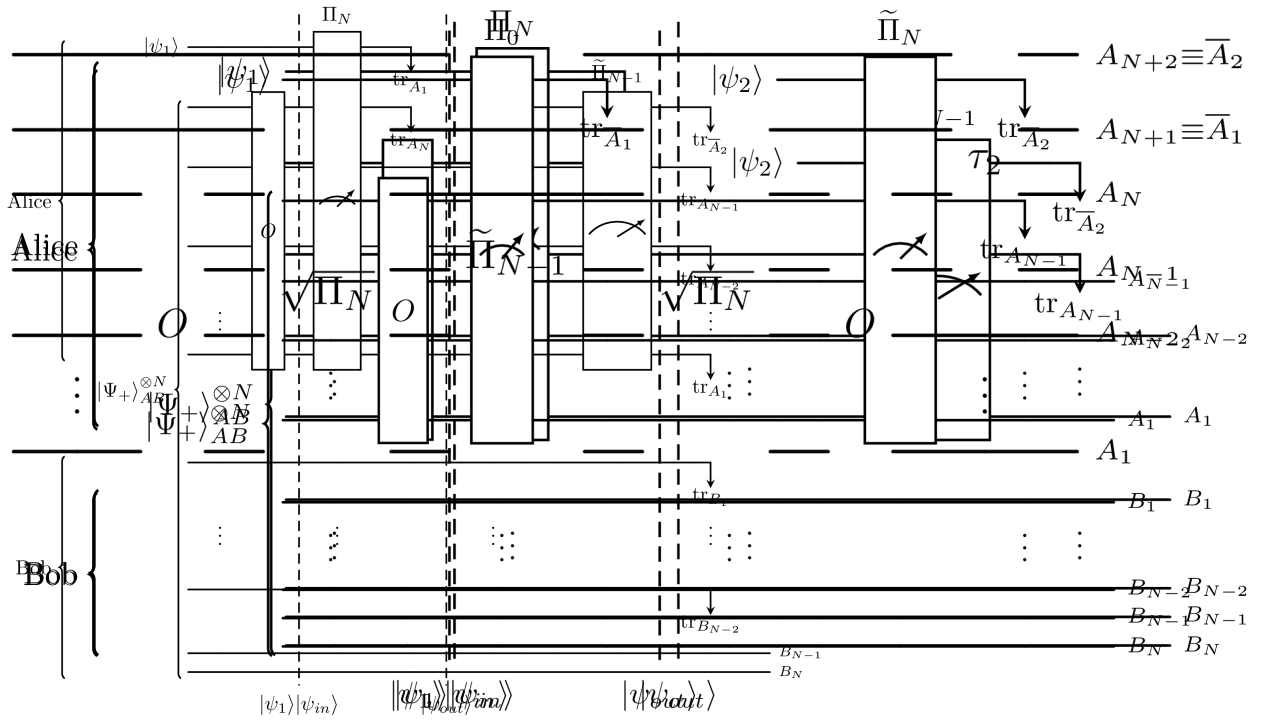
Figure 1. Two-step PBT Protocol at a glance: Initially, Alice and Bob share the optimized resource state $\lvert{\Psi}\rangle=(O_{A}\otimes I_{B})\lvert{\Psi^{+}}\rangle_{AB}$. Alice performs the POVM $\Pi$ on her registers $A_{1},\ldots,A_{N},\bar{A}_{1},\bar{A}_{2}$, where the state $\lvert{\psi_{1}}\rangle$ which she wants to teleport is in the $\bar{A}_{1}$th register. If she succeeds and measures the outcome $i\neq 0$, the state $\lvert{\psi_{1}}\rangle$ is perfectly teleported to Bob’s register $i_{B}$. By discarding the ports $A_{i}$ and $B_{i}$ along with register $\bar{A}_{1}$, Alice and Bob share recycled state $\lvert{\psi_{\text{rec}}}\rangle$ on $N-1$ registers on each side. In this paper we study the usefulness of state $\lvert{\psi_{\text{rec}}}\rangle$ for for a second round of the protocol. In the second round, Alice performs joint POVM $\widetilde{\Pi}$ on registers $(\{A_{1},\ldots,A_{N}\}\setminus A_{i})\cup\bar{A}_{2}$, where register $\bar{A}_{2}$ contains another state $\lvert{\psi_{2}}\rangle$ that she wants to teleport. Measuring the outcome $j\neq 0$ in this round indicates success. The figure shows a situation where Alice obtains outcome $N$ in the first measurement and $N-1$ in the second.

2. Summary of the results

2.1. Degradation of the resource state after the first round of pPBT

In the first part of the paper the degradation of the resource state after one round of probabilistic protocol is studied. The reasoning is such, that if the degradation is vanishing in the limit of $N$, then the resource can be reused, provided it is sufficiently large. The measure of degradation of the resource state is state fidelity $F$ between the actual resource after one round of teleportation $\Psi^{(i)}_{\mathrm{out}}$, and an idealised state $\Psi_{\mathrm{id}}^{(i)}$ that is perfectly suitable for the subsequent teleportation, where $i$ dentotes the measurement obtained by Alice

$$F^{\mathrm{rec}}(N,d,1)=\sum_{i=0}^{N}p_{i}F(\Psi_{\mathrm{out}}^{(i)},\Psi_{\mathrm{id}}^{(i)}),$$ (1)

namely if no degradation to the ports apart from the one where the teleportation occurred is present, this quantity is equal to 1. Due to the probabilistic nature of the protocol, one is interested in conditional state fidelity

$$F^{\mathrm{rec}}_{\mathrm{succ}}(N,d,1)=\frac{\sum_{i=1}^{N}p_{i}F(\Psi_{\mathrm{out}}^{(i)},\Psi_{\mathrm{id}}^{(i)})}{\sum_{i=1}^{N}p_{i}}$$ (2)

and

$$F^{\mathrm{rec}}_{\mathrm{fail}}(N,d,1)=\frac{p_{0}F(\Psi_{\mathrm{out}}^{(0)},\Psi_{\mathrm{id}}^{(0)})}{p_{0}}.$$ (3)

since it is reasonable to ask about the usefulness of the resource in both cases. One has to note though, that in case of the failure, obviously the first state is not teleported, so the case of two following rounds is of greater interest (and it is studied in greater detail in second part of the paper).

The above quantities are evaluated in two variations of pPBT protocol - one that employs EPR pairs as a resource state, and the other that uses optimised resource (see Section 3.2 for the detailed description of both variants). The conclusion can be drawn only in the former case: since $F^{\mathrm{rec}}_{\mathrm{succ}}$ goes to 1 when $N\to\infty$ (see Section 4.1), while $p_{0}\to 0$, one can say, that total state fidelity goes to 1. For the latter variant no such reasoning can be made: the state fidelity tends to some number between 1 and 0, disabling a conclusion concerning the suitability of the resource for future uses - it can be either useful or not. However, the discussion presented in the second part of the article provides meaningful information about that scenario.

2.2. Direct evaluation of the quantities describing the protocol

Since one cannot directly asses the amount of degradation in the remaining resource, the problem can be reformulated. Namely, view the succeeding executions of pPBT protocol that use the same resource, as a single protocol that teleports two quantum states, just with some possible time delay between the two instances of teleportation. One can observe, that thus the recycling protocol is a subclass of multi port-based teleportation protocols. The study shows that indeed, in asymptotic limit two quantities characterising the channel $\mathcal{N}:\operatorname{End}(\bar{A}_{1}\otimes\bar{A}_{2})\to\operatorname{End}(\bar{B}_{1}\otimes\bar{B}_{2})$

$$\begin{split}\mathcal{N}(\rho_{\bar{A}}):=&\sum_{i=1}^{N}\sum_{\begin{subarray}{c}j=1\\ j\neq i\end{subarray}}^{N}\operatorname{Tr}_{A\bar{B}^{c}_{ij}\bar{A}}\left[\sqrt{\widetilde{\Pi}_{j}}{\sqrt{\Pi_{i}}}(\Psi_{AB}\otimes\rho_{\bar{A}}){\sqrt{\Pi_{i}}}\sqrt{\widetilde{\Pi}_{j}}\right]_{B_{i},B_{j}\to\bar{B}_{1},\bar{B}_{2}}\end{split}$$ (4)

where $B^{c}_{ij}:=B/\{B_{i},B_{j}\}$, associated with two successful subsequent teleportations, and thus the performance of the protocol, namely the probability of success in two subsequent teleportations

$$p_{\mathrm{succ}}(\mathcal{N})\vcentcolon=\operatorname{Tr}\mathcal{N}_{\bar{A}_{1}\bar{A}_{2}\to\bar{B}_{1}\bar{B}_{2}}(I/d)$$ (5)

and entanglement fidelity

$$F_{e}(\mathcal{N})\vcentcolon=\operatorname{Tr}\left[\psi^{+}_{\bar{B}_{1}R_{1}}\otimes\psi^{+}_{\bar{B}_{2}R_{2}}\big{\lparen}\mathcal{N}_{\bar{A}_{1}\bar{A}_{2}\to\bar{B}_{1}\bar{B}_{2}}\otimes I_{R_{1}R_{2}}\big{\rparen}\big{\lparen}\psi^{+}_{\bar{A}_{1}R_{1}}\otimes\psi^{+}_{\bar{A}_{2}R_{2}}\big{\rparen}\right]$$ (6)

indicate that the two step teleportation is efficient, since $p_{\mathrm{succ}}(\mathcal{N})\xrightarrow[N\to\infty]{}1$ as well as for the conditional entanglement fidelity $F_{e}(\mathcal{N})/p_{\mathrm{succ}}\xrightarrow[N\to\infty]{}1$. What is more, it is shown that the expression for $p_{\mathrm{succ}}$ coincides with the optimal probability of success in MPBT for two teleported states. In fact the approach to concentrate on the case of success in the first step is sound, since it is known that the probability of failure in pPBT vanishes with the increase of the size of the resource [IH09, SSMH17, Chr+20].

In fact, since both optimal pPBT protocol and both variants of dPBT protocol employ closely related set of measurements (in fact, in dPBT the effect corresponding to failure in pPBT is distributed between effects from 1 to $N$), this method can be employed to asses the entanglement fidelity of recycling in deterministic scheme, enabling its comparison to MPBT protocols, something that has not been done earlier (only the qualitative statement that the resource in the limit of large $N$ is suitable for subsequent teleportation, without specifying exact entanglement fidelity for finite $N$ [SMK22]). This discussion is presented in the last paragraph 6.

3. Preliminaries

3.1. Representation theory of the partially transposed permutation algebra

The setting of our problem is naturally suited for using tools from mixed Schur–Weyl duality for the matrix algebra of partially transposed permutations. Here we present a summary of necessary results, and we refer the reader to [GBO23] for more details. Some aspects of the representation theory of partially transposed permutation matrix algebras were also studied before in [SHM13, MHS14, MSH18]

The matrix algebra $\mathcal{A}^{d}_{N,2}$ of partially transposed permutations acts on $N+2$ qudits, each of local dimension $d$. Its generators $\sigma_{1},\dotsc,\sigma_{N+1}$ act on $(\mathbb{C}^{d})^{\otimes N+2}$ in the following way: for all $x_{1},\dotsc,x_{N+2}\in[d]\vcentcolon=\{1,\dotsc,d\}$,

$$\sigma_{i}\,\lvert{x_{1},\dotsc,x_{N+2}}\rangle\vcentcolon=\begin{cases}\lvert{x_{1},\dotsc,x_{i+1},x_{i},\dotsc,x_{N+2}}\rangle,&\text{$i\neq N$},\\ \lvert{x_{1},\dotsc,x_{N-1}}\rangle\otimes(\delta_{x_{N},x_{N+1}}\sum_{k=1}^{d}\lvert{k,k}\rangle)\otimes\lvert{x_{N+2}}\rangle,&\text{$i=N$}.\end{cases}$$ (7)

In other words, $\sigma_{i}$ with $i\neq N$ are transpositions that exchange qudits $i$ and $i+1$, while $\sigma_{N}$ is a contraction that projects the last two qudits on the un-normalized maximally entangled state. The irreducible representations or irreps of $\mathcal{A}_{N,2}^{d}$ are labelled by the following pairs of Young diagrams of four types:

$$\widehat{\mathcal{A}}_{N,2}^{d}\vcentcolon=\Big{\{}(\nu,\varnothing)\nonscript\>\Big{|}\allowbreak\nonscript\>\mathopen{}\nu\mathbin{\vdash}_{d}N-2\Big{\}}\sqcup\Big{\{}(\lambda,\leavevmode\hbox to7.51pt{\vbox to7.51pt{\text{[drawing]}}})\nonscript\>\Big{|}\allowbreak\nonscript\>\mathopen{}\lambda\mathbin{\vdash}_{d-1}N-1\Big{\}}\sqcup\Big{\{}(\mu,\leavevmode\hbox to5.38pt{\vbox to10.36pt{\text{[drawing]}}})\nonscript\>\Big{|}\allowbreak\nonscript\>\mathopen{}\mu\mathbin{\vdash}_{d-2}N\Big{\}}\sqcup\Big{\{}(\mu,\leavevmode\hbox to10.36pt{\vbox to5.38pt{\text{[drawing]}}})\nonscript\>\Big{|}\allowbreak\nonscript\>\mathopen{}\mu\mathbin{\vdash}_{d-1}N\Big{\}},$$ (8)

where $\varnothing$ denotes the empty diagram and $\square=(1)$. More generally, the irreducible representations of $\mathcal{A}_{N,M}^{d}$ for arbitrary $N,M\geqslant 0$ are labelled by pairs of partitions $\Lambda=(\lambda,\lambda^{\prime})$ such that $\ell(\lambda)+\ell(\lambda^{\prime})\leqslant d$ and $\lambda\mathbin{\vdash}N-k$ and $\lambda^{\prime}\mathbin{\vdash}M-k$ for some $0\leqslant k\leqslant\min(N,M)$ [GBO23] (in our case $M=2$ and $k=0,1,2$). We slightly abuse notation by not including $d$ as part of $\Lambda$ since $d$ is assumed to be fixed throughout. However, knowing $d$ is necessary to unambiguously convert $\Lambda$ into a staircase of length $d$, which is another convenient way of labelling the irreps of $\mathcal{A}_{N,M}^{d}$ [Ste87, GBO23].

Description of representation theory of $\mathcal{A}_{N,2}^{d}$, is based on the notion of Bratteli diagram $\mathscr{B}$ for the sequence of algebras $\mathcal{A}_{0,0}^{d}\hookrightarrow\mathcal{A}_{1,0}^{d}\hookrightarrow\cdots\hookrightarrow\mathcal{A}_{N,0}^{d}\hookrightarrow\mathcal{A}_{N,1}^{d}\hookrightarrow\mathcal{A}_{N,2}^{d}$, which is a certain directed acyclic simple graph [GBO23]. The vertices of $\mathscr{B}$ are divided into $N+3$ levels denoted by $i=0,\dotsc,N+2$. These levels correspond to sets of irreducible representations $\widehat{\mathcal{A}}_{0,0}^{d},\widehat{\mathcal{A}}_{1,0}^{d},\dotsc,\widehat{\mathcal{A}}_{N,2}^{d}$ of the corresponding algebras $\mathcal{A}_{0,0}^{d},\mathcal{A}_{1,0}^{d},\dotsc,\mathcal{A}_{N,2}^{d}$. The vertices at level $i\in\{0,\dotsc,N\}$ are labelled by Young diagrams $\lambda\mathbin{\vdash}_{d}i$, while the vertices at the last levels $N+1,N+2$ are labelled by pairs of Young diagrams $\Lambda$ corresponding to the irreps of $\widehat{\mathcal{A}}_{N,1}^{d}$ and $\widehat{\mathcal{A}}_{N,2}^{d}$ , see eq.˜8. When $i\in\{0,\dotsc,N\}$, the vertices $\mu\,\mathbin{\vdash}\,i-1$ and $\lambda\,\mathbin{\vdash}\,i$ are connected, denoted as $\mu\rightarrow\lambda$, if $\lambda$ can be obtained from $\mu$ by adding a cell, i.e., $\lambda=\mu\cup a$ for some $a\in\mathrm{AC}_{d}(\mu)$. Furthermore, for levels $\geqslant N$ vertices at consequtive levels are connected by adding a cell to right Young diagram $\Lambda_{r}$ or removing a cell from $\Lambda_{l}$. The Bratteli diagram $\mathscr{B}$ consists of all vertices from all levels and the directed edges between them. We denote the only vertex at level $0$ by $\varnothing$ and call it root, while the vertices at the last level of $\mathscr{B}$ we call leaves (they correspond bijectively to the irreps $\widehat{\mathcal{A}}_{N,2}^{d}$). For any leaf $\Lambda\in\widehat{\mathcal{A}}_{N,2}^{d}$, we denote by

$$\mathrm{Paths}(\Lambda,\mathscr{B})\vcentcolon=\Big{\{}T=(T^{0}\to T^{1}\to\dotsc\to T^{N+1}\to T^{N+1})=(T^{0},T^{1},\dotsc,T^{N+1},T^{N+1})\Big{\}}$$ (9)

the set of all paths in $\mathscr{B}$ starting at the root $T^{0}=\varnothing$ and terminating at $\Lambda$. For any path $T=(T^{0},\dotsc,T^{N+2})\in\mathrm{Paths}(\Lambda,\mathscr{B})$ and $i\in[N+1]$ we define the walled content of $i$ in $T$ as

$$\mathrm{wcont}_{i}(T)\vcentcolon=\begin{cases}\mathrm{cont}(T^{i}_{l}\setminus T^{i-1}_{l})&\text{if }i\leqslant N,\\ \mathrm{cont}(T^{i}_{r}\setminus T^{i-1}_{r})+d&\text{if }i>N\text{ and }T^{i}_{l}=T^{i-1}_{l},\\ -\mathrm{cont}(T^{i-1}_{l}\setminus T^{i}_{l})&\text{if }i>N\text{ and }T^{i}_{r}=T^{i-1}_{r}.\end{cases}$$ (10)

where content of a cell $c=(i,j)$ is given by $\mathrm{cont}(c)\vcentcolon=j-i$, and the axial distance between $i$ and $i+1$ in $T$ as

$$r_{i}(T)=\mathrm{wcont}_{i+1}(T)-\mathrm{wcont}_{i}(T).$$ (11)

Similar to eq.˜9, for any intermediate vertex $\lambda\mathbin{\vdash}k$ at level $k\leqslant N$ in $\mathscr{B}$, we use $\mathrm{Paths}_{k}(\lambda,\mathscr{B})$ to denote the set of all paths in $\mathscr{B}$ terminating at $\lambda$. Furthermore, we denote by $\mathrm{Paths}(\mathscr{B})$ the set of all paths in $\mathscr{B}$, i.e., $\mathrm{Paths}(\mathscr{B})\vcentcolon=\bigsqcup_{\Lambda\in\widehat{\mathcal{A}}_{N,2}^{d}}\mathrm{Paths}(\Lambda,\mathscr{B})$.

For a given $\Lambda\in\widehat{\mathcal{A}}_{N,2}^{d}$, the corresponding irrep $\psi_{\Lambda}$ has a convenient explicit description in the so-called Gelfand–Tsetlin basis $\{\lvert{T}\rangle\mid T\in\mathrm{Paths}(\Lambda,\mathscr{B})\}$. Recall from eq.˜7 that $\mathcal{A}_{N,2}^{d}$ is generated by $N$ transpositions $\sigma_{1},\dotsc,\sigma_{N-1},\sigma_{N+1}$ and one contraction $\sigma_{N}$. For any irrep $\Lambda\in\widehat{\mathcal{A}}_{N,2}^{d}$, a transposition $\sigma_{i}$ acts on a given path $T\in\mathrm{Paths}(\Lambda,\mathscr{B})$ as follows:

$$\psi_{\Lambda}(\sigma_{i})\,\lvert{T}\rangle =\frac{1}{r_{i}(T)}\,\lvert{T}\rangle+\sqrt{1-\frac{1}{r_{i}(T)^{2}}}\,\lvert{\sigma_{i}T}\rangle\qquad\text{for $i\neq N$},$$ (12)

where $\sigma_{i}T$ denotes the path $T$ with vertex $T^{i}$ at level $i$ replaced by $T^{i-1}\cup(T^{i+1}\setminus T^{i})$. This is known as Young–Yamanouchi formula. The action of $\sigma_{N}$ is given by (see [GBO23, Theorem 3.2]) for every irrep $\Lambda$ and a valid path from $\mathrm{Paths}_{N-1}((\lambda,\varnothing),\mathscr{B})$:

$$\psi_{\Lambda}(\sigma_{n})\,\lvert{S\to(\lambda\cup a)\to(\lambda,\varnothing)\to\Lambda}\rangle =\sum_{a^{\prime}\in\mathrm{AC}_{d}(\lambda)}\frac{\sqrt{m_{\lambda\cup a}m_{\lambda\cup a^{\prime}}}}{m_{\lambda}}\lvert{S\to(\lambda\cup a^{\prime})\to(\lambda,\varnothing)\to\Lambda}\rangle,$$ (13)

where $m_{\lambda}$ denotes the dimension of the $\lambda$-irrep of the unitary group $\mathrm{U}_{d}$. Finally, according to the well-known Weyl dimension formula, the dimension of unitary group irrep labelled by a general staircase $\Lambda$ is given by

$$m_{\Lambda}=\prod_{1\leqslant i<j\leqslant d}\frac{\Lambda_{i}-\Lambda_{j}+j-i}{j-i}.$$ (14)

3.2. Optimal measurements and resource states for pPBT

In the probabilistic port-based teleportation scheme (pPBT) two parties share $N$ entangled pairs, each of local dimension $d$, and the subsystems are labeled by $A\vcentcolon=A_{1},\dots,A_{N}$ and $B\vcentcolon=B_{1},\dots,B_{N}$. The register corresponding to the state to be teleported is denoted by $\bar{A}_{1}$. In order to teleport an unknown state $\rho_{\bar{A}_{1}}$, the first party (Alice) performs a measurement on systems $C$ and $A$. The measurement outcomes labeled by $1$ to $N$ are then communicated to the second party (Bob) to indicate at which port the desired state is teleported. This state is referred to as $\bar{B}_{1}$. The additional measurement result labeled $0$ corresponds to the failure of the entire procedure.

Depending on the shared resource and the measurements applied by Alice, one can distinguish two types of pPBT protocol: the standard and optimized.

3.2.1. Standard pPBT

In the standard scenario the shared state consists of $N$ EPR pairs $\lvert{\psi^{+}}\rangle=\frac{1}{\sqrt{d}}\sum_{i=1}^{d}\lvert{ii}\rangle$, i.e.

$$\lvert{\Psi^{+}}\rangle_{AB}\vcentcolon=\bigotimes_{i=1}^{N}\lvert{\psi^{+}}\rangle_{A_{i}B_{i}}.$$ (15)

The joint measurement $\Pi=\{\Pi_{i}\}_{i=0}^{N}$ in question, due to the symmetries present in the problem [IH08] takes the form

$$\Pi_{i}=\psi^{+}_{A_{i}\bar{A}_{1}}\otimes\Theta_{i^{c}},\quad\Theta_{i^{c}}=\sum_{\lambda\vdash_{d}N-1}\frac{d}{\gamma(\lambda)}P^{i^{c}}_{\lambda}\quad i=1,\dots,N,\quad\Pi_{0}=I-\sum_{i=1}^{N}\Pi_{i}$$ (16)

where the bar in $\Theta_{i^{c}}$ says that the operator acts everywhere but $i$, $\psi^{+}_{A_{i}\bar{A}_{1}}$ is a density matrix of the maximally entangled state supported on subsystems labelled $A_{i}$ and $\bar{A}_{1}$ and

$$\gamma(\lambda) \vcentcolon=\max_{\begin{subarray}{c}a\in\mathrm{AC}(\lambda)\end{subarray}}\gamma_{a}(\lambda)=d+\lambda_{1},\quad\gamma_{a}(\lambda)\vcentcolon=d+\mathrm{cont}{(a)},$$ (17)

and

$$P_{\lambda}=\sum_{S\in\mathrm{Paths}_{N-1}{(\lambda)}}\lvert{S}\rangle\langle{S}\rvert$$ (18)

is a projector onto irrep $\lambda$ in $\left(\mathbb{C}^{d}\right)^{\otimes{N-1}}$, while the superscript $i^{c}$ in $P_{\lambda}^{i^{c}}$ means it is supported on systems $A_{1},\dots,A_{i-1},A_{i+1},\dots,A_{N}$. The effects $\Pi_{i}$ for $i=1,\dots,N$ correspond to successful teleportation to the $i$-th port, while the remaining effect $\Pi_{0}$ corresponds to the failure of the whole procedure.

3.2.2. Optimal pPBT

When Alice performs optimization over resource state, it is of the form [IH09, MSSH18]

$$\lvert{\Psi}\rangle_{AB}=\bigl{(}O_{A}\otimes I_{B}\bigr{)}\lvert{\Psi^{+}}\rangle_{AB},\quad O_{A}=\sum_{{\mu}\vdash_{d}N}\sqrt{c_{\mu}}P_{\mu},$$ (19)

where

$$c_{\mu}\vcentcolon=\frac{d^{N}g(N)m_{\mu}}{d_{\mu}},\quad g(N)\vcentcolon=\frac{1}{\sum_{\mu\mathbin{\vdash}_{d}N}m_{\mu}^{2}}=\frac{1}{\binom{N+d^{2}-1}{d^{2}-1}}$$ (20)

In the Gelfand-Tsetlin basis, the optimized state can be written with the help of mixed Schur transform as [GBO24]:

$$U_{\text{mSch}}\lvert{\Psi}\rangle_{AB}=\sum_{\mu\vdash_{d}N}\sqrt{f_{\mu}}\lvert{\mathrm{EPR}^{[n-1]}_{\mu}}\rangle\lvert{\mu}\rangle_{T^{N}},$$ (21)

where

$$f_{\mu}\vcentcolon=\frac{c_{\mu}d_{\mu}m_{\mu}}{d^{N}},\quad f_{\mu}=\frac{m_{\mu}^{2}}{\sum_{\nu\mathbin{\vdash}_{d}N}m_{\nu}}$$ (22)

and

$$\lvert{\mathrm{EPR^{[n-1]}_{\mu}}}\rangle\vcentcolon=\sum_{S\in\mathrm{Paths}_{N}(\mu)}\sqrt{\frac{1}{d_{\mu}}}\lvert{S_{0}\to\dotsb\to S_{n-1}}\rangle_{T^{0},\dotsc,T^{n-1}}\lvert{S_{n-1}\to\dotsb\to S_{0}}\rangle_{T^{n+1},\dotsc,T^{2n}}$$ (23)

The optimal pPBT measurement [SSMH17] is

$$\Pi_{i}=O_{A}^{-1}\big{\lparen}\psi^{+}_{A_{i}\bar{A}_{1}}\otimes\sum_{\lambda\vdash_{d}N-1}u_{\lambda}P_{\lambda}^{i^{c}}\big{\rparen}(O_{A}^{\dagger})^{-1},\quad i=1,\dots,N$$ (24)

where

$$u_{\lambda}\vcentcolon=\frac{d^{N+1}g(N)m_{\lambda}}{Nd_{\lambda}}.$$ (25)

The above effects correspond to teleportation to $i$-th port, whereas the remaining one, $\Pi_{0}=I-\sum_{i=1}^{N}\Pi_{i}$ corresponds to the failure of the whole procedure.

The POVM $\Pi$ turns out to be a so-called Pretty Good Measurement (PGM) given by

$$\Pi_{i} \vcentcolon=\rho^{-1/2}\rho_{i}\rho^{-1/2},\quad\rho\vcentcolon=\sum_{i=1}^{N}\rho_{i},\quad\rho_{i}\vcentcolon=R((i,N))\sigma_{N}R((i,N)),\quad\quad\Pi_{0}\vcentcolon=I-\sum_{i=1}^{n}\Pi_{i},$$ (26)

where $(i,N)$ is the permutation, which swaps $i$ and $N$ systems, and $R$ is the tensor representation of $\operatorname{S}_{N}$ on ${(\mathbb{C}^{d})}^{\otimes(N+1)}$. Notice that $\rho$ commutes with $\operatorname{S}_{N}$, hence the POVM elements $\Pi_{i}$ for $i\in[N]$ can be written as

$$\Pi_{i}=R((i,N))\Pi_{N}R((i,N)),$$ (27)

hence the POVM $\Pi$ is group-covariant [DJR04] with respect to the cyclic group on $N$ elements.

We now present a useful description of SRM eq.˜26 the in Gelfand–Tsetlin basis. For each irrep $\Lambda$, we denote by $\Pi_{k}^{\Lambda}$ an operator $\Pi_{k}$ restricted to the irrep $\Lambda$:

$$U_{\mathrm{Sch}}\Pi_{k}U_{\mathrm{Sch}}^{\dagger}=\bigoplus_{\Lambda\in\widehat{\mathcal{A}}_{N,2}^{d}}\Pi_{k}^{\Lambda}\otimes I_{m_{\Lambda}},$$ (28)

where $I_{m_{\Lambda}}$ are identity matrices acting on the registers, corresponding to unitary group irreps. The irreducible $\Lambda$ symbols are labeled by pairs of Young diagrams of four types. We are interested mostly in $\Lambda=(\lambda,\varnothing)$ where $\lambda\mathbin{\vdash}_{d}N-1$ type.

One knows the representations of $\sigma_{N}$ and $\rho^{-1/2}$ as elements of $\mathcal{A}_{N,1}^{d}$ [GBO24]:

$$\sigma_{N}^{\Lambda}=\begin{cases}\sum_{S\in\mathrm{Paths}(\lambda)}\sum_{a,a^{\prime}\in\mathrm{AC}_{d}(\lambda)}\frac{\sqrt{m_{\lambda\cup a}m_{\lambda\cup a^{\prime}}}}{m_{\lambda}}\lvert{S\to\lambda\cup a\to(\lambda,\varnothing)}\rangle\langle{S\to\lambda\cup a\to(\lambda,\varnothing)}\rvert&\text{if $\Lambda=(\lambda,\varnothing)$},\\ 0&\text{if $\Lambda=(\mu,\square)$},\\ \end{cases}$$ (29)

and

$$(\rho^{-1/2})^{\Lambda}=\begin{cases}\sum_{a\in\mathrm{AC}_{d}(\lambda)}\sum_{T\in\mathrm{Paths}(\lambda\cup a)}\frac{1}{\sqrt{d+\mathrm{cont}{(a)}}}\lvert{T\to(\lambda,\varnothing)}\rangle\langle{T\to(\lambda,\varnothing)}\rvert&\text{if $\Lambda=(\lambda,\varnothing)$},\\ 0&\text{if $\Lambda=(\mu,\square)$}.\\ \end{cases}$$ (30)

By embedding the above elements into $\mathcal{A}_{N,2}^{d}$, we get the following result:

Lemma 1.

The POVM element $\Pi_{N}^{\Lambda}$ in any irrep $\Lambda\in\widehat{\mathcal{A}}_{N,2}^{d}$ can be expressed as:

$$\Pi_{N}^{\Lambda}=\sum_{\lambda\mathbin{\vdash}_{d}N-1}\sum_{S\in\mathrm{Paths}(\lambda)}G_{\lambda,S}\,\sigma_{N}^{\Lambda}\,G_{\lambda,S}$$ (31)

where

$$G_{\lambda,S}=\sum_{a\in\mathrm{AC}_{d}(\lambda)}\frac{1}{\sqrt{d+\mathrm{cont}{(a)}}}\lvert{S\to\lambda\cup a}\rangle\langle{S\to\lambda\cup a}\rvert\otimes I$$ (32)

Notice that matrices $G_{\lambda,S}$ does not depend on $\Lambda\in\widehat{\mathcal{A}}_{N,2}^{d}$

Proof.

Direct calculation using formulas eqs.˜29 and 30. Notice that although matrices $G_{\lambda,S}$ have non-trivial support on irreps $\Lambda=(\mu,\leavevmode\hbox to7.51pt{\vbox to7.51pt{\text{[drawing]}}})$ at level $N+1$, however, $\sigma_{N}^{\Lambda}$ is supported only on irreps $\Lambda=(\lambda,\varnothing)$ at level $N+1$ of the Bratteli diagram for $\mathcal{A}_{N,2}^{d}$. ∎

Moreover, in the future the following lemma is useful for calculations:

Lemma 2 ([GBO23]).

For any partition $\lambda=(\lambda_{1},\dotsc,\lambda_{d})\mathbin{\vdash}N-1$ and $a\in\mathrm{AC}(\lambda)$ we have

$$N\frac{d_{\lambda}}{m_{\lambda}}\frac{m_{\lambda\cup a}}{d_{\lambda\cup a}}=d+\mathrm{cont}{(a)}$$ (33)

4. Degradation of the resource state in probabilistic port-based teleportation

The quantity of interest is how well the resource state is preserved after one (and possibly more) round of teleportation scheme. Precisely, we are interested in recycling fidelity, i.e. the overlap between the actual state after the measurement $\Psi_{\mathrm{out}}^{(i)}$ and the idealised one $\Psi_{\mathrm{id}}^{(i)}$, i.e. one that corresponds to no resource degradation at all

$$F^{\mathrm{rec}}(N,d,1)=\sum_{i=0}^{N}p_{i}F(\Psi_{\mathrm{out}}^{(i)},\Psi_{\mathrm{id}}^{(i)})=\sum_{i=0}^{N}p_{i}\frac{\operatorname{Tr}(\lvert{\Psi_{\mathrm{out}}^{(i)}}\rangle\langle{\Psi_{\mathrm{id}}^{(i)}}\rvert)}{\lVert\lvert{\Psi_{\mathrm{out}}^{(i)}}\rangle\rVert_{2}},$$ (34)

where $i$ corresponds to possible measurement outcomes and hence various post-measurement states. One can in particular discuss conditional recycling fidelity

$$F^{\mathrm{rec}}_{\mathrm{succ}}(N,d,1)=\frac{\sum_{i=1}^{N}p_{i}F(\Psi_{\mathrm{out}}^{(i)},\Psi_{\mathrm{id}}^{(i)})}{\sum_{i=1}^{N}p_{i}}=F(\Psi_{\mathrm{out}}^{(N)},\Psi_{\mathrm{id}}^{(N)})$$ (35)

and

$$F^{\mathrm{rec}}_{\mathrm{fail}}(N,d,1)=\frac{p_{0}F(\Psi_{out}^{(0)},\Psi_{id}^{(0)})}{p_{0}}=F(\Psi_{out}^{(0)},\Psi_{id}^{(0)}),$$ (36)

where the last equality in (35) follows from the covariance of the protocol with respect to action of $S(N)$ group, which simply means that the teleportation characteristics cannot depend on the port, where the teleported state arrives. Thus, the quantities of interest are overlap of the post measurement states with the corresponding idealised states.

4.1. Degradation of resource state in standard pPBT

In the standard scheme the input state is

$$\lvert{\Psi_{\mathrm{in}}}\rangle=\lvert{\Psi^{+}}\rangle_{AB}\otimes\lvert{\psi^{+}}\rangle_{\bar{A}_{1}R_{1}}.$$ (37)

where $\lvert{\psi^{+}}\rangle_{\bar{A}_{1}R_{1}}$ is a maximally entangled state, half of which is teleported by Alice to Bob. The idealised state corresponding to the teleportation to ith port reads

$$\lvert{\Psi_{\mathrm{id}}^{(i)}}\rangle=\bigotimes_{j\neq i}\lvert{\psi^{+}}\rangle_{{A_{j}}{B_{j}}}\otimes\lvert{\psi^{+}}\rangle_{{\bar{A}_{1}}{A_{i}}}\otimes\lvert{\psi^{+}}\rangle_{{R_{1}}{B_{i}}}.$$ (38)

Whenever the teleportation finishes with failure the idealised state is just the initial state

$$\lvert{\Psi_{id}^{(0)}}\rangle=\lvert{\Psi^{+}}\rangle_{AB}\otimes\lvert{\psi^{+}}\rangle_{\bar{A}_{1}R_{1}}.$$ (39)

4.1.1. Conditional fidelity after success

From [SMK22] we know the following relation

$$R((i,N))\sigma_{N}R((i,N))^{\dagger}\otimes I_{B{R_{1}}}\lvert{\Psi_{\mathrm{in}}}\rangle=\lvert{\Psi_{\mathrm{id}}^{(i)}}\rangle.$$ (40)

For the maximally entangled resource state

$$\operatorname{Tr}\lvert{\Psi_{\mathrm{id}}^{(i)}}\rangle\langle{\Psi_{\mathrm{out}}^{(i)}}\rvert=\frac{1}{d^{N+1}}\operatorname{Tr}\left(\sqrt{\Pi_{i}}R((i,N))\sigma_{N}R((i,N))^{\dagger}\right).$$ (41)

The normalization term is

$$\left|\left|\sqrt{\Pi^{\bar{A}_{1}A}_{i}}\otimes I_{R_{1}B}\lvert{\Psi_{\mathrm{in}}}\rangle\right|\right|_{2}= \frac{1}{\sqrt{d^{N+1}}}\left(\operatorname{Tr}{\Pi_{i}}\right)^{1/2}$$ (42)

Due to the covariance (see (35)) we are interested only in the calculation for $i=N$. The expression for recycling fidelity thus becomes

$$F^{\mathrm{rec}}_{\mathrm{succ}}(N,1,d)=\frac{1}{\sqrt{d^{N+1}}}\frac{\operatorname{Tr}(\sqrt{\Pi_{N}}\sigma_{N})}{\sqrt{\operatorname{Tr}{\Pi_{N}}}}.$$ (43)

Theorem 3.

The conditional recycling fidelity in the case of success after one round of pPBT protocol is given by

$$F^{\mathrm{rec}}_{\mathrm{succ}}=\frac{1}{\sqrt{d^{N-1}}}\frac{\sum_{\lambda\vdash_{d}N-1}\sqrt{\frac{1}{\gamma(\lambda)}}m_{\lambda}d_{\lambda}}{\sqrt{\sum_{\lambda}\frac{1}{\gamma(\lambda)}m_{\lambda}d_{\lambda}}}.$$ (44)

Proof.

The measurement in question is given by (16) and is a pseudo-projector and thus its square root is given by

$$\sqrt{\Pi_{N}}=\sum_{\lambda\vdash_{d}N-1}\psi_{\bar{A}_{1},A_{N}}^{+}\otimes\sqrt{\frac{d}{\gamma(\lambda)}}P_{\lambda}^{{N^{c}}}.$$ (45)

Thus the expression for $\operatorname{Tr}(\sqrt{\Pi_{N}}\sigma_{N})$ becomes

$$\operatorname{Tr}(\sqrt{\Pi_{N}}\sigma_{N}) =d\sum_{\lambda\vdash_{d}N-1}\sqrt{\frac{d}{\gamma(\lambda)}}\operatorname{Tr}(\psi^{+}_{\bar{A}_{1},A_{N}}\otimes P_{\lambda})$$ (46)

$$=d\sum_{\lambda\vdash_{d}N-1}\sqrt{\frac{d}{\gamma(\lambda)}}m_{\lambda}d_{\lambda}$$ (47)

and similarly

$$\operatorname{Tr}\Pi_{N}=\sum_{\lambda\vdash_{d}N-1}\frac{d}{\gamma(\lambda)}m_{\lambda}d_{\lambda}$$ (48)

which, substituted to (43) gives the statement of the Theorem. ∎

4.1.2. Conditional fidelity after failure

The idealized state in the event of failure is the initial resource state, because one assumes that no teleportation takes place $\lvert{\Psi^{(0)}_{\mathrm{id}}}\rangle=\lvert{\Psi^{+}_{AB}}\rangle$. Thus, the overlap between actual post-failure resource and idealized one is

$$F(\lvert{\Psi^{(0)}_{\mathrm{id}}}\rangle,\lvert{\Psi^{(0)}_{\mathrm{out}}}\rangle)=\frac{1}{\sqrt{d^{N+1}}}\frac{\operatorname{Tr}\sqrt{\Pi_{0}}}{\sqrt{\operatorname{Tr}\Pi_{0}}}.$$ (49)

The effect $\Pi_{0}$ is an element of algebra of partially transposed permutation operators $\mathcal{A}_{N,1}^{d}$. It is given by $\Pi_{0}=I-G$ (see [GBO24]) and

$$G=\sum_{\lambda\mathbin{\vdash}_{d}N-1}\sum_{a\in\mathrm{AC}_{d}(\lambda)}g_{\lambda,a}\Pi_{\lambda,a}\quad\Pi_{\lambda,a}=\sum_{S\in\mathrm{Paths}_{N}{(\lambda\cup{a})}}\lvert{S\to(\lambda,\varnothing)}\rangle\langle{S\to(\lambda,\varnothing)}\rvert.$$ (50)

Since $\operatorname{Tr}\Pi_{\lambda,a}=m_{\lambda}d_{\lambda\cup{a}}$, one has

$$\operatorname{Tr}{\Pi_{0}}=d^{N+1}-\sum_{\lambda\mathbin{\vdash}_{d}N-1}\sum_{a\in\mathrm{AC}_{d}{(\lambda)}}g_{\lambda,a}m_{\lambda}d_{\lambda\cup{a}}.$$ (51)

as well as

$$\operatorname{Tr}\sqrt{\Pi_{0}}={d^{N+1}-\sum_{\lambda\mathbin{\vdash}_{d}N-1}\sum_{a\in\mathrm{AC}_{d}{(\lambda)}}(1-\sqrt{1-g_{\lambda,a}})m_{\lambda}d_{\lambda\cup{a}}}.$$ (52)

The expressions (51),(52) lead to

Theorem 4.

The conditional recycling fidelity in the case of failure is standard pPBT protocol is given by

$$F^{\mathrm{rec}}_{\mathrm{fail}}=\frac{1}{\sqrt{d^{N+1}}}\frac{\operatorname{Tr}\sqrt{\Pi_{0}}}{\sqrt{\operatorname{Tr}\Pi_{0}}}=\frac{1-\frac{1}{d^{N+1}}\sum_{\lambda\mathbin{\vdash}_{d}N-1}\sum_{a\in\mathrm{AC}_{d}{(\lambda)}}(1-\sqrt{1-g_{\lambda,a}})m_{\lambda}d_{\lambda\cup{a}}}{\sqrt{1-\frac{1}{d^{N+1}}\sum_{\lambda\mathbin{\vdash}_{d}N-1}\sum_{a\in\mathrm{AC}_{d}{(\lambda)}}g_{\lambda,a}m_{\lambda}d_{\lambda\cup{a}}}}.$$ (53)

where

$$g_{\lambda,a}\vcentcolon=\frac{\gamma_{a}(\lambda)}{\gamma(\lambda)}=\frac{d+\mathrm{cont}(a)}{d+\lambda_{1}}$$ (54)

4.1.3. Summary for the standard pPBT

The numerical results regarding conditional recycling fidelity both in case of the success and failure are depicted in Figure 2.

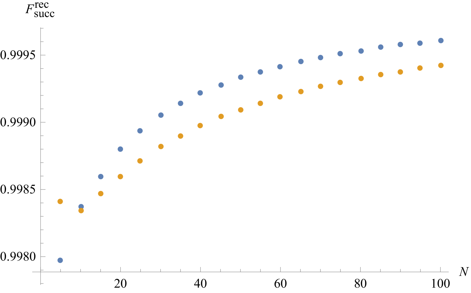
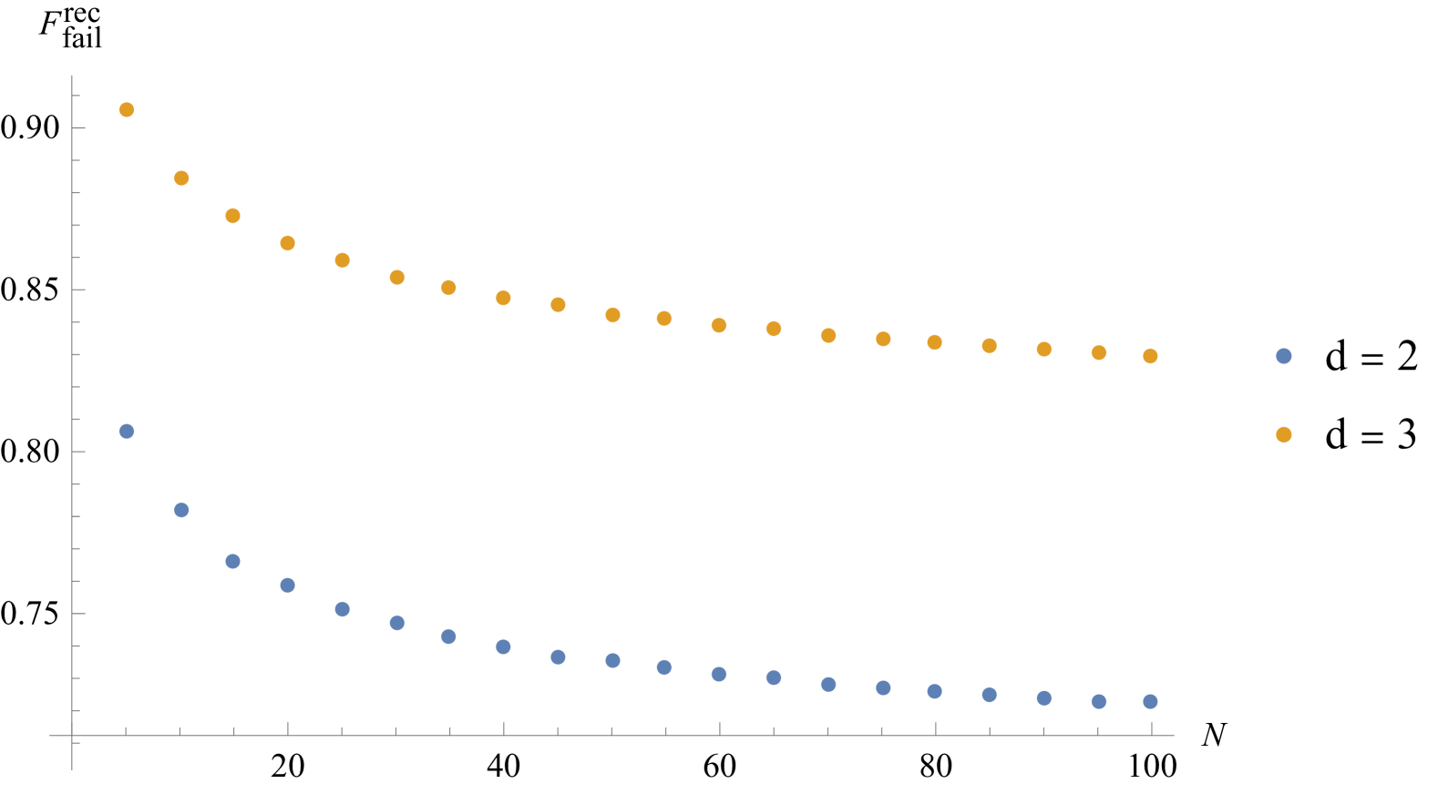
Figure 2. Conditional recycling fidelity for success (left) and failure (right) in standard pPBT scheme, for $d=2$ (blue dots) and $d=3$ (orange dots)

Provided that the first round of the teleportation succeeds, allowing for arbitrarily large resources, the resulting resource state converges to the ideal state. In that case, the remaining ports can be reused for another round of pPBT. In the case of failure, the problem is unresolved - one cannot infer whether the remaining resource is sufficient for further application of the standard pPBT protocol. However, it is known [IH09, SSMH17, Chr+20] that $p_{\mathrm{fail}}=1-p_{\mathrm{succ}}\to 0$ when $N\to\infty$. This means that in total $\lim_{N\to\infty}F_{rec}(N,d,1)=\lim_{N\to\infty}F_{succ}^{rec}(N,d,1)$, meaning that for an arbitrarily large resource state one can reuse the resource state after performing one round of the standard pPBT protocol.

4.2. Degradation of resource state in optimal pPBT

Conditional fidelity after success

In the case of the success of the teleportation procedure, the idealized state is given by

$$\lvert{\Psi_{\mathrm{id}}^{(i)}}\rangle=\psi^{+}_{{\bar{A}_{1}}{A_{i}}}\otimes\psi^{+}_{{R_{1}}{B_{i}}}\otimes\bigl{(}O_{\widetilde{A}}\otimes I\bigr{)}\bigotimes_{j\neq i}\psi^{+}_{{A_{j}}{B_{j}}}$$ (55)

which can be written as

$$\lvert{\Psi_{\mathrm{id}}^{(i)}}\rangle=R((i,N))\sigma_{N}R((i,N))^{\dagger}\lvert{\psi^{+}_{\bar{A}_{1}R_{1}}}\rangle\lvert{\psi^{+}_{A_{i}B_{i}}}\rangle\otimes\bigl{(}O_{\widetilde{A}}\otimes I\bigr{)}\bigotimes_{j\neq i}\psi^{+}_{{A_{j}}{B_{j}}}$$ (56)

whereas the actual unnormalized outcome state is

$$\lvert{\Psi_{\mathrm{out}}^{(i)}}\rangle=\sqrt{\Pi_{i}}\bigl{(}(O_{A}\otimes I_{B})\lvert{\Psi^{+}}\rangle_{AB}\otimes\lvert{\psi^{+}_{\bar{A}_{1}R_{1}}}\rangle\bigr{)}.$$ (57)

Due to the covariance of the protocol, see (35), one can restrict oneself to the study of one effect, namely $\Pi_{N}$. The overlap between the idealized and the unnormalized outcome resource state (for $i=N$) is then given by

$$F(\Psi_{\mathrm{out}}^{(N)},\Psi_{\mathrm{id}}^{(N)})=\frac{1}{\sqrt{d^{N+1}}}\frac{\operatorname{Tr}(\sigma_{N}\sqrt{\Pi_{N}}O_{A}O_{\widetilde{A}})}{\sqrt{\operatorname{Tr}(\Pi_{N}O_{A}O_{A}})}$$ (58)

where $O_{\widetilde{A}}$ is an optimization operator that acts on $\widetilde{A}=1,\dots,N-1$.

One can observe that the expression (58) is of the same form as an expression for the overlap in optimal dPBT scheme [SMK22]. The measurement in the optimal pPBT scheme is closely related to POVMs in standard and optimized dPBT schemes, up to the additional factor $\Delta=\Pi_{0}/N$, which does not contribute to the quantity since it is orthogonal to $\sigma_{N}$. The quantity is thus the same, up to different coefficients of the optimization procedure $O_{A},O_{\widetilde{A}}$. Thus, the quantity in question is described by the following Theorem:

Theorem 5.

The recycling fidelity after success in one round of optimal pPBT is given by

$$F^{\mathrm{rec}}_{\mathrm{succ}}=\frac{1}{d^{\frac{N+1}{2}}}\Bigl{(}\sum_{\lambda,a\in\mathrm{AC}_{d}(\lambda)}c_{\lambda}^{1/2}c_{\lambda\cup{a}}^{1/2}\frac{d_{\lambda}\sum_{a^{\prime}\in\mathrm{AC}_{d}(\lambda)}\sqrt{m_{\lambda\cup{a^{\prime}}}d_{\lambda\cup{a^{\prime}}}}}{\sqrt{\sum_{a\in\mathrm{AC}_{d}(\lambda)}d_{\lambda\cup{a}}}}\frac{\sqrt{m_{\lambda\cup{a}}d_{\lambda\cup{a}}}}{\sqrt{Nd_{\lambda}}}\Bigr{)}\Bigl{/}\sqrt{\sum_{\lambda}u_{\lambda}d_{\lambda}m_{\lambda}}.$$ (59)

Conditional fidelity after failure In case of optimal protocol, the idealised state is

$$\lvert{\Psi_{id}}\rangle=(O_{A}\otimes I_{B})\lvert{\Psi^{+}}\rangle_{AB}\lvert{\psi^{+}_{\bar{A}_{1}R_{1}}}\rangle.$$ (60)

and the (unnormalised) post-measurement state

$$\lvert{\Psi_{out}^{(0)}}\rangle=\sqrt{\Pi_{0}}\bigl{(}(O_{A}\otimes I_{B})\lvert{\Psi^{+}}\rangle_{AB}\otimes\lvert{\psi^{+}_{\bar{A}_{1}R_{1}}}\rangle\bigr{)}$$ (61)

Since [GBO24] the effect $\Pi_{0}$ is identity in irreps $(\mu,\square)$ and zero in other ones, one has the following expression for the overlap

$$\operatorname{Tr}(\lvert{\Psi_{id}}\rangle\langle{\Psi_{out}}\rvert)= \operatorname{Tr}(O_{A}\lvert{\psi^{+}_{AB}}\rangle\lvert{\psi^{+}_{\bar{A}_{1}R_{1}}}\rangle\langle{\psi^{+}}\rvert_{AB}\langle{\psi^{+}}\rvert_{\bar{A}_{1}R_{1}}O_{A}^{\dagger}\sqrt{\Pi_{0}})$$ (62)

$$= \frac{1}{d^{N+1}}\operatorname{Tr}(O_{A}O_{A}^{\dagger}\sqrt{\Pi_{0}})=\sum_{\mu\vdash_{d-1}N}\frac{c_{\mu}}{d^{N+1}}\operatorname{Tr}(P_{\mu}M_{(\mu,\square)})$$ (63)

where $M_{(\mu,\square)}$ is a projection onto irrep $(\mu,\square)$. Since $\operatorname{Tr}(P_{\mu}M_{(\mu,\square)})=m_{(\mu,\square)}d_{\mu}$, and the normalisation factor is

$$\begin{split}||\lvert{\Psi_{out}}\rangle||=\frac{1}{\sqrt{d^{N+1}}}\Bigl{(}\sum_{\mu\vdash_{d-1}N}c_{\mu}\operatorname{Tr}(P_{\mu}M_{(\mu,\square)})\Bigr{)}^{1/2}\end{split}$$ (64)

one obtains fhe following

Theorem 6.

The recycling fidelity in case of failure after one round of optimal pPBT protocol is given by

$$F^{\mathrm{rec}}_{\mathrm{fail}}=\frac{1}{\sqrt{d^{N+1}}}\Bigl{(}\sum_{\mu\vdash_{d-1}N}c_{\mu}m_{(\mu,\square)}d_{\mu}\Bigr{)}^{1/2}$$ (65)

Summary for the optimal pPBT The numerical results regarding conditional recycling fidelity both in case of the success and failure are depicted in Figure 3

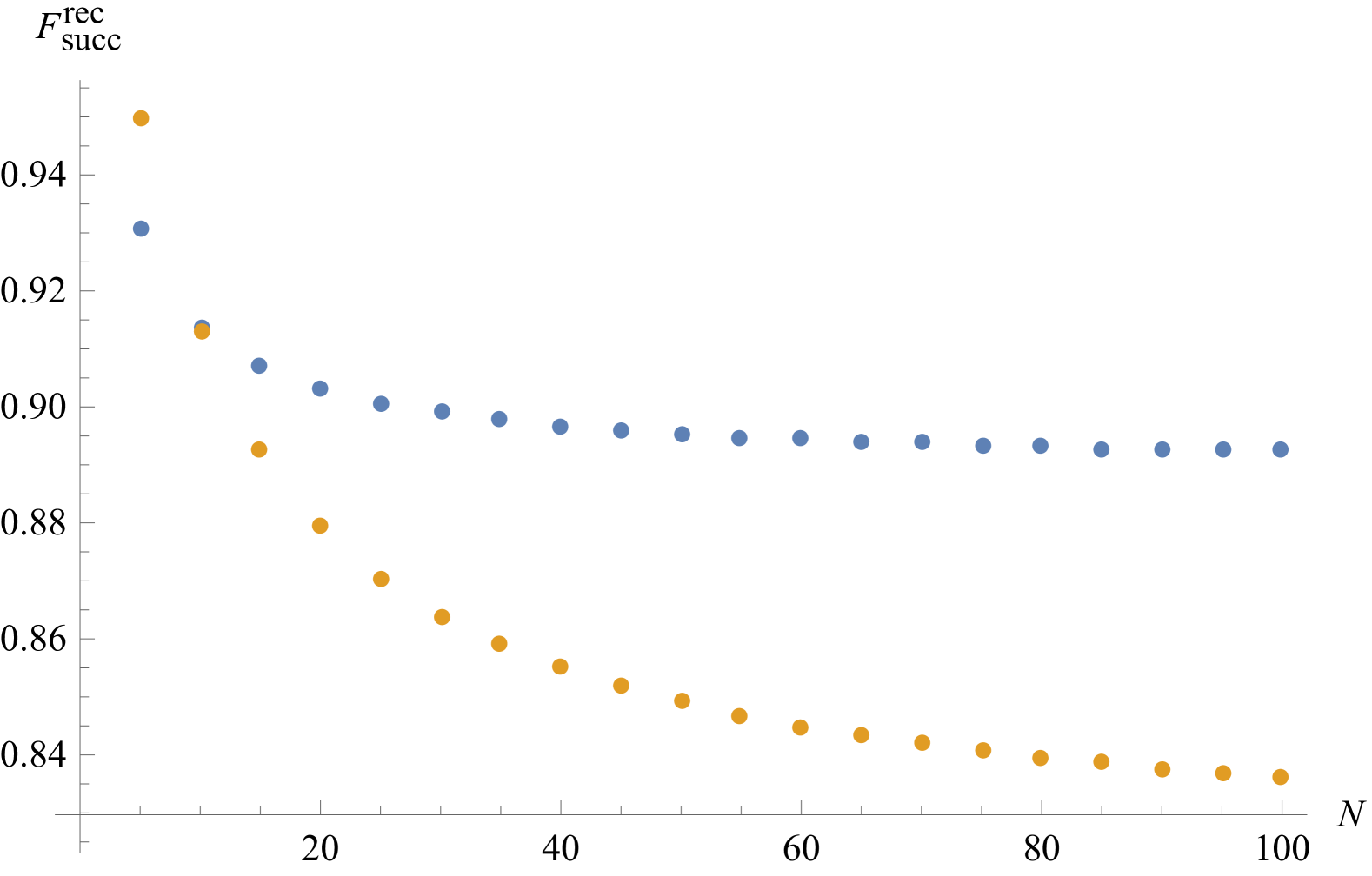
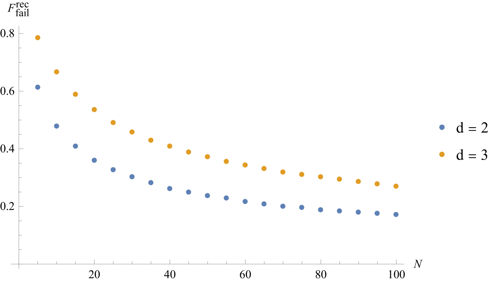
Figure 3. Conditional recycling fidelity for success (left) and failure (right) in optimal pPBT scheme, for $d=2$ (blue dots) and $d=3$ (orange dots).

The resulting values do not determine whether the outcome states in any of the cases (success or failure) allow for effective application of the successive round of pPBT.

5. Entanglement fidelity of two-step pPBT

Since no definite answer could be provided by the analysis of the degradation of the resource state after one execution of optimal pPBT protocol, the problem can be rephrased. The succeeding performance of successful executions of the protocol (i.e. such that neither the first, nor the second measurement outcome indicates failure) can be viewed as a protocol that teleports two quantum states. Thus, the examination of the quantities describing its performance give information about potential usefulness of the resource state that was employed to succesfully teleport one quantum state, to teleport another one.

Recall that $A=\{A_{1},\ldots,A_{N}\}$ are the registers on Alice’s side which store a part of the resource state, and $B=\{B_{1},\ldots,B_{N}\}$ are the registers on Bob’s side, while registers $\bar{A}=\{\bar{A}_{1},\bar{A}_{2}\}$ correspond to state register which Alice wants to teleport. Alice and Bob share an optimized resource state

$$\lvert{\Psi}\rangle_{AB}\vcentcolon=O_{A}\otimes I_{B}\lvert{\Psi^{+}}\rangle_{AB}$$ (66)

while registers $\bar{A}$ on Alice’s side contain a state $\rho_{\bar{A}}$, consisting of two qudits, that Alice wants to teleport. We denote the density matrix corresponding to the state $\lvert{\Psi}\rangle_{AB}$ by $\Psi_{AB}$.

The first POVM is denoted by $\Pi=\{\Pi_{0},\ldots,\Pi_{N}\}$ and is performed by Alice on registers in $A\cup\bar{A}_{1}$. If Alice measures $i\neq 0$ (success in the first round), the post-measurement state is denoted by

$$\Psi^{(i)}_{\mathrm{out}}\vcentcolon=\frac{\operatorname{Tr}_{A_{i}B_{i}\bar{A}_{1}}[\sqrt{\Pi_{i}}(\Psi_{AB}\otimes\rho_{\bar{A}})\sqrt{\Pi_{i}}]}{\operatorname{Tr}{[\Pi_{i}(\Psi_{AB}\otimes\rho_{\bar{A}})}]}.$$ (67)

Alice might then perform a second POVM, denoted by $\widetilde{\Pi}=\{\widetilde{\Pi}_{0},\ldots,\widetilde{\Pi}_{N-1}\}$, on the registers $(A\setminus A_{i})\cup\bar{A}_{2}$ (see Fig.˜1).

Denote by $\mathcal{N}:\mathcal{H}_{d}^{\otimes 2}\rightarrow\mathcal{H}_{d}^{\otimes 2}$ the conditional quantum channel

$$\begin{split}\mathcal{N}(\rho_{\bar{A}}):=&\sum_{i=1}^{N}\sum_{\begin{subarray}{c}j=1\\ j\neq i\end{subarray}}^{N}\operatorname{Tr}_{A\bar{B}^{c}_{ij}\bar{A}}\left[\sqrt{\widetilde{\Pi}_{j}}{\sqrt{\Pi_{i}}}(\Psi_{AB}\otimes\rho_{\bar{A}}){\sqrt{\Pi_{i}}}\sqrt{\widetilde{\Pi}_{j}}\right]_{B_{i},B_{j}\to\bar{B}_{1},\bar{B}_{2}}\end{split}$$ (68)

where $\bar{B}^{c}_{ij}:=B/\{B_{i},B_{j}\}$, which describes the post-measurement state in case of success ($i,j\neq 0$) in both rounds of the protocol. Notice that channel $\mathcal{N}$ is not trace preserving, as it does not contain elements $\Pi_{0},\widetilde{\Pi}_{0}$.

The probability of success of this channel is defined by

$$p_{\text{succ}}\vcentcolon=\operatorname{Tr}\mathcal{N}(I/d^{2}).$$ (69)

The entanglement fidelity of such a channel can be computed by

$$F_{e}(\mathcal{N})\vcentcolon=\operatorname{Tr}\left[\psi^{+}_{\bar{B}_{1}R_{1}}\otimes\psi^{+}_{\bar{B}_{2}R_{2}}\left\lparen\mathcal{N}_{\bar{A}_{1}\bar{A}_{2}\to\bar{B}_{1}\bar{B}_{2}}\otimes I_{R_{1}R_{2}}\right\rparen\left\lparen\psi^{+}_{\bar{A}_{1}R_{1}}\otimes\psi^{+}_{\bar{A}_{2}R_{2}}\right\rparen\right]$$ (70)

where $R_{1},R_{2}$ are auxiliary registers, and $\psi^{+}_{XY}$ are maximally entangled states shared between $X$ and $Y$ registers.

Since the measurements $\Pi,\widetilde{\Pi}$ are covariant under the action of $\operatorname{S}_{N}$, $\operatorname{S}_{N-1}$ respectively

$$R(\sigma)\Pi_{i}R(\sigma)^{\dagger}=\Pi_{\sigma(i)},\quad\sigma\in\operatorname{S}_{N}$$ (71)

$$R(\sigma^{\prime})\widetilde{\Pi}_{j}R(\sigma^{\prime})^{\dagger}=\widetilde{\Pi}_{\sigma^{\prime}(j)},\quad\sigma^{\prime}\in\operatorname{S}_{N-1}$$ (72)

Calculating $F_{e}(\mathcal{N})$ can be interpreted as contracting a tensor network obtained from the circuit in Fig.˜1. In particular, it is easy to see that by bending wires of Fig.˜1, $F_{e}(\mathcal{N})$ can be transformed into taking trace of the operator as in Fig.˜4. Therefore, the entanglement fidelity of the channel (68) reads

$$F_{e}(\mathcal{N})=\frac{N(N-1)}{d^{N+2}}\operatorname{Tr}\left[O_{A}\sqrt{\Pi_{N}}\widetilde{\Pi}_{N-1}\;\sqrt{\Pi_{N}}\;O_{A}\;\tau_{2}\right]$$ (73)

where $\Pi_{N},\widetilde{\Pi}_{N-1}$ are POVMs elements, $O_{A}$ corresponds to the preparation of the optimal state, and

$$\tau_{2}\vcentcolon=d^{2}(I_{A_{1},\dots,A_{N-2}}\otimes{\psi^{+}}_{A_{N}\bar{A}_{1}}\otimes{\psi^{+}}_{A_{N-1}\bar{A}_{2}})$$ (74)

is an unnormalized projector onto two EPR pairs. In the following, it makes sense to call registers $\bar{A}_{1},\bar{A}_{2}$ as $A_{N+1},A_{N+2}$, see Fig.˜4.

$F_{e}(\mathcal{N})=\frac{N(N-1)}{d^{N+4}}\operatorname{Tr}\left[{4}\leavevmode\hbox{$\vbox{\hbox{\resizebox{}{}{{\leavevmode\hbox{\set@color{}}}}}}$}\right]$

Figure 4. Entanglement fidelity of the channel $\mathcal{N}$ can written as a tensor network contraction by bending and rearranging the wires and tensors from Fig.˜1.

5.1. Entanglement fidelity calculation in the Gelfand–Tsetlin basis

In this section we derive the formula for the entanglement fidelity $F_{e}(\mathcal{N})$ of the channel $\mathcal{N}$ presented in eq.˜73. By the cyclic property of trace, we have

$$F_{e}(\mathcal{N})=\frac{N(N-1)}{d^{N+4}}\operatorname{Tr}_{A}\Big{(}\sqrt{\Pi_{N}}\;\widetilde{\Pi}_{N-1}\;\sqrt{\Pi_{N}}\;O\;\tau_{2}\;O\Big{)}$$ (75)

As all elements are unitary-equivariant, we may express all elements of (73) in the Gelfand-Tsetlin basis. Therefore (75) reads

$$F_{e}(\mathcal{N})=\frac{N(N-1)}{d^{N+4}}\sum_{\Lambda\in\widehat{\mathcal{A}}_{N,2}^{d}}m_{\Lambda}\operatorname{Tr}\left[\sqrt{\Pi_{N}^{\Lambda}}\;\widetilde{\Pi}_{N-1}\;\sqrt{\Pi_{N}^{\Lambda}}\;O^{\Lambda}\;\tau_{2}^{\Lambda}\;O^{\Lambda}\right]$$ (76)

where $m_{\Lambda}$ is the dimension of the corresponding unitary irrep, and $\tau_{2}^{\Lambda}$ is an irrep $\Lambda$ of $\tau_{2}$ from eq.˜74. Notice that, since $\Pi_{N}^{\Lambda},\;\widetilde{\Pi}_{N-1}^{\Lambda}$ are supported only on irreps $\Lambda=(\nu,\varnothing)$, the only contributions to the formula (76) are from those irreps. Therefore (76) reads:

$$F_{e}(\mathcal{N}) =\frac{N(N-1)}{d^{N+4}}\sum_{\nu\mathbin{\vdash}_{d}N-2}m_{\nu}\operatorname{Tr}\left[\widetilde{\Pi}_{N-1}^{(\nu,\varnothing)}\;\sqrt{\Pi_{N}^{(\nu,\varnothing)}}\;O^{(\nu,\varnothing)}\;\tau_{2}^{(\nu,\varnothing)}\;O^{(\nu,\varnothing)}\;\sqrt{\Pi_{N}^{(\nu,\varnothing)}}\right]$$ (77)

We shall derive formulas for each element in (77).

Firstly, notice that

$$(\sqrt{\Pi_{N}})^{(\nu,\varnothing)}=\sum_{a\in\mathrm{AC}_{d}(\nu)}\sum_{r\in\mathrm{RC}(\nu\cup a)}\sum_{S\in\mathrm{Paths}(\nu\cup a/r)}\frac{\lvert{w^{\nu}_{S,r,a}}\rangle\langle{{w^{\nu}_{S,r,a}}}\rvert}{||\lvert{w^{\nu}_{S,r,a}}\rangle||}$$ (78)

where

$$\lvert{w^{\nu}_{S,r,a}}\rangle=\sum_{b\in\mathrm{AC}_{d}(\nu\cup a)}\sqrt{\frac{d_{\nu\cup a\cup b}}{Nd_{\nu\cup a}}}\lvert{S\to\nu\cup a\to\nu\cup a\cup b\to(\nu\cup a,\varnothing)\to(\nu,\varnothing)}\rangle$$ (79)

Secondly, we express $\widetilde{\Pi}_{N-1}$ using formula (31), namely we have

$$\widetilde{\Pi}_{N-1}^{\Lambda}=\sum_{\nu\mathbin{\vdash}_{d}N-2}\sum_{S\in\mathrm{Paths}(\nu)}G_{\nu,S}\,(U^{\Lambda}\,\sigma_{N}^{\Lambda}\,U^{\Lambda})\,G_{\nu,S}$$ (80)

where $U^{\Lambda}=\sigma_{N-1}^{\Lambda}\sigma_{N+1}^{\Lambda}$ and hence $U=U^{\dagger}$ and $(U^{\Lambda}\sigma_{N}^{\Lambda}U^{\Lambda})$ is a contraction between $N-1$ and $N+2$, and

$$G_{\nu,S}=\sum_{a\in\mathrm{AC}_{d}(\nu)}\frac{1}{\sqrt{d+\mathrm{cont}{(a)}}}\lvert{S\to\nu\cup a}\rangle\langle{{S\to\nu\cup a}}\rvert\otimes I^{\otimes 3}$$ (81)

Notice that element $\sigma_{N}^{\Lambda}$ for $\Lambda=(\nu,\varnothing)$ has the following form

$$\sigma_{N}^{(\nu,\varnothing)}=\sum_{a\in\mathrm{AC}_{d}(\nu)}\sum_{r\in\mathrm{RC}(\nu\cup a)}\sum_{S\in\mathrm{Paths}(\nu\cup a/r)}\frac{\lvert{\widetilde{v^{\nu}_{S,r,a}}}\rangle\langle{\widetilde{v^{\nu}_{S,r,a}}}\rvert}{||\lvert{\widetilde{v^{\nu}_{S,r,a}}}\rangle||}(\sigma_{N-1}\sigma_{N+1})^{(\nu,\varnothing)}$$ (82)

where

$$\lvert{\widetilde{v^{\nu}_{S,r,a}}}\rangle=\sum_{b\in\mathrm{AC}_{\nu\cup a}}\sqrt{\frac{m_{\nu\cup a\cup b}}{m_{\nu\cup a}}}\lvert{S\to\nu\cup a\to\nu\cup a\cup b\to(\nu\cup a,\varnothing)\to(\nu,\varnothing)}\rangle$$ (83)

Thirdly, we compute

$$O^{(\nu,\varnothing)}\;\tau_{2}^{(\nu,\varnothing)}\;O^{(\nu,\varnothing)}=\sum_{S\in\mathrm{Paths}_{N-2}(\nu)}\lvert{v^{\nu}_{S}}\rangle\langle{v^{\nu}_{S}}\rvert$$ (84)

where

$$\lvert{v^{\nu}_{S}}\rangle=\sum_{a\neq b\in\mathrm{AC}_{d}(\nu)}\sqrt{c_{\nu\cup a\cup b}}\sqrt{\frac{m_{\nu\cup a\cup b}}{m_{\nu}}}\lvert{S\to\nu\cup a\to\nu\cup a\cup b\to(\nu\cup a,\varnothing)\to(\nu,\varnothing)}\rangle.$$ (85)

Lastly, we denote by

$$\lvert{\widetilde{w_{S,a,a}^{\nu}}}\rangle:=G_{\nu,S}\lvert{w_{S,a,a}^{\nu}}\rangle=\sum_{b\in\mathrm{AC}_{d}(\nu\cup a)}\sqrt{\frac{d_{\nu\cup a\cup b}}{Nd_{\nu\cup a}(d+\mathrm{cont}(a))}}\lvert{S\to\nu\cup a\to\nu\cup a\cup b\to(\nu\cup a,\varnothing)\to(\nu,\varnothing)}\rangle.$$ (86)

Combining formulas in eqs.˜78, 79, 80, 81, 82, 83, 84, 85 and 86, (77) become

$$F_{e}(\mathcal{N})=\frac{N(N-1)}{d^{N+4}}\sum_{\nu\mathbin{\vdash}_{d}N-2}d_{\nu}m_{\nu}\cdot\\ \sum_{\begin{subarray}{c}a,a^{\prime},a^{\prime\prime}\\ \in\mathrm{AC}_{d}(\nu)\end{subarray}}\sum_{\begin{subarray}{c}r\in\mathrm{RC}(\nu\cup a)\\ r^{\prime}\in\mathrm{RC}(\nu\cup a^{\prime})\\ r^{\prime\prime}\in\mathrm{RC}(\nu\cup a^{\prime\prime})\end{subarray}}\frac{\langle{v_{S}^{\nu}}|{w_{S,a,r}^{\nu}}\rangle}{||w_{S,a,r}^{\nu}||}\langle{\widetilde{w_{S,a,r}^{\nu}}}|{U^{(\nu,\varnothing)}|\widetilde{v_{S,a^{\prime},r^{\prime}}^{\nu}}}\rangle\langle{\widetilde{v_{S,a^{\prime},r^{\prime}}^{\nu}}}|{U^{(\nu,\varnothing)}|\widetilde{w_{S,a^{\prime\prime},r^{\prime\prime}}^{\nu}}}\rangle\frac{\langle{w_{S,a^{\prime\prime},r^{\prime\prime}}^{\nu}}|{v_{S}^{\nu}}\rangle}{||w_{S,a^{\prime\prime},r^{\prime\prime}}^{\nu}||}$$ (87)

Notice that $\langle{w_{S,a,r}^{\nu}}|{v_{S}^{\nu}}\rangle=0$ for $a\neq r$, hence (87) become

$$F_{e}(\mathcal{N})=\frac{N(N-1)}{d^{N+4}}\sum_{\nu\mathbin{\vdash}_{d}N-2}d_{\nu}m_{\nu}\sum_{\begin{subarray}{c}a,a^{\prime},a^{\prime\prime}\\ \in\mathrm{AC}_{d}(\nu)\end{subarray}}\frac{\langle{v_{S}^{\nu}}|{w_{S,a,a}^{\nu}}\rangle}{||w_{S,a,a}^{\nu}||}\langle{\widetilde{w_{S,a,a}^{\nu}}}|{U^{(\nu,\varnothing)}|\widetilde{v_{S,a^{\prime},a^{\prime}}^{\nu}}}\rangle\langle{\widetilde{v_{S,a^{\prime},a^{\prime}}^{\nu}}}|{U^{(\nu,\varnothing)}|\widetilde{w_{S,a^{\prime\prime},a^{\prime\prime}}^{\nu}}}\rangle\frac{\langle{w_{S,a^{\prime\prime},a^{\prime\prime}}^{\nu}}|{v_{S}^{\nu}}\rangle}{||w_{S,a^{\prime\prime},a^{\prime\prime}}^{\nu}||}$$ (88)

Now we compute overlaps in (88). Firstly notice that from (79) and (81)

$$\langle{v_{S}^{\nu}}|{w_{S,a,a}^{\nu}}\rangle=\sum_{b\in\mathrm{AC}_{d}(\nu\cup a)}\sqrt{\frac{d_{\nu\cup a\cup b}}{Nd_{\nu\cup a}}}\sqrt{c_{\nu\cup a\cup b}}\sqrt{\frac{m_{\nu\cup a\cup b}}{m_{\nu}}}$$ (89)

And further using the definition of $c_{\nu\cup a\cup b}$, see eq.˜20, we arrive at

$$\langle{v_{S}^{\nu}}|{w_{S,a,a}^{\nu}}\rangle=\sqrt{\frac{d^{N}}{Nd_{\nu\cup a}m_{\nu}}}\Big{\lparen}\sum_{b\in\mathrm{AC}_{d}(\nu\cup a)}\sqrt{f_{\nu\cup a\cup b}}\Big{\rparen}$$ (90)

For optimal pPBT state we have, using eq.˜20, we have

$$\langle{v_{S}^{\nu}}|{w_{S,a,a}^{\nu}}\rangle=\Big{\lparen}\sum_{b\in\mathrm{AC}_{d}(\nu\cup a)}m_{\nu\cup a\cup b}\Big{\rparen}\sqrt{\frac{d^{N}g(N)}{Nd_{\nu\cup a}m_{\nu}}}=d\,m_{\nu\cup a}\sqrt{\frac{d^{N}g(N)}{Nd_{\nu\cup a}m_{\nu}}}.$$ (91)

Secondly, we have that

$$\langle{\widetilde{w_{S,a,a}^{\nu}}}|{U^{(\nu,\varnothing)}|\widetilde{v_{S,a^{\prime},a^{\prime}}^{\nu}}}\rangle=\sum_{\begin{subarray}{c}b\in\mathrm{AC}(\nu\cup a)\\ b^{\prime}\in\mathrm{AC}(\nu\cup a^{\prime})\end{subarray}}\frac{1}{\sqrt{d+\mathrm{cont}{(a)}}}\sqrt{\frac{d_{\nu\cup a\cup b}m_{\nu\cup a^{\prime}\cup b^{\prime}}}{d_{\nu\cup a}m_{\nu\cup a^{\prime}}}}\langle{\begin{subarray}{c}S\to\nu\cup a\to\nu\cup a\cup b\to\\ \to(\nu\cup a,\varnothing)\to(\nu,\varnothing)\end{subarray}}\rvert U\lvert{\begin{subarray}{c}S\to\nu\cup a^{\prime}\to\nu\cup a^{\prime}\cup b^{\prime}\to\\ \to(\nu\cup a^{\prime},\varnothing)\to(\nu,\varnothing)\end{subarray}}\rangle.$$ (92)

Notice that non-vanishing contributions to such expressions are if and only if $\{a,b\}=\{a^{\prime},b^{\prime}\}$, hence we can distinguish two cases: either $a=a^{\prime}$ and $b=b^{\prime}$, or $b=a^{\prime}\neq a=b^{\prime}$. Utilizing Young–Yamanouchi basis formulas for $U=\sigma_{N-1}^{\Lambda}\sigma_{N+1}^{\Lambda}$, we arrive at:

$$\langle{\widetilde{w_{S,a,a}^{\nu}}}|{U^{(\nu,\varnothing)}|\widetilde{v_{S,a^{\prime},a^{\prime}}^{\nu}}}\rangle=\begin{cases}\sum_{b\in\mathrm{AC}_{d}(\nu\cup a)}\frac{m_{\nu\cup a\cup b}}{m_{\nu\cup a}}\frac{1}{\sqrt{(d+\mathrm{cont}{(a)})(d+\mathrm{cont}{(b)})}}\frac{1}{(\mathrm{cont}{(a)-\mathrm{cont}{(b)}})^{2}}&\text{if $a=a^{\prime}\in\mathrm{AC}_{d}(\nu)$},\\ \frac{m_{\nu\cup a\cup a^{\prime}}}{\sqrt{m_{\nu\cup a}m_{\nu\cup a^{\prime}}}}\frac{1}{\sqrt{(d+\mathrm{cont}{(a)})(d+\mathrm{cont}{(a^{\prime})})}}\Big{(}1-\frac{1}{(\mathrm{cont}{(a)-\mathrm{cont}{(a^{\prime})}})^{2}}\Big{)}&\text{if $a\neq a^{\prime}\in\mathrm{AC}_{d}(\nu)$}.\end{cases}$$ (93)

After rewriting of eq.˜87, we get the expression:

$$F_{e}(\mathcal{N}) =\frac{1}{d^{4}}\sum_{\nu\mathbin{\vdash}_{d}N-2}\sum_{\begin{subarray}{c}a,a^{\prime},a^{\prime\prime}\in\mathrm{AC}_{d}(\nu)\end{subarray}}\sum_{\mu,\mu^{\prime\prime}\mathbin{\vdash}_{d}N}v_{\mu}S^{\nu}_{a,\mu}H^{\nu}_{a,a^{\prime}}H^{\nu}_{a^{\prime},a^{\prime\prime}}S^{\nu}_{a^{\prime\prime},\mu^{\prime\prime}}v_{\mu^{\prime\prime}}=v^{\mathsf{T}}Mv,$$ (94)

where the vector $v$ has components labelled every partition $\mu\mathbin{\vdash}_{d}N$:

$$v_{\mu} \vcentcolon=\sqrt{f_{\mu}},$$ (95)

and the matrices $H^{\nu},S^{\nu}$ and $M$ are defined as

$$H^{\nu}_{a,a^{\prime}} \vcentcolon=\begin{dcases}\sum_{b\in\mathrm{AC}_{d}(\nu\cup a)}\sqrt{\frac{d+\mathrm{cont}(b)}{d+\mathrm{cont}(a)}}\frac{q(b|\nu\cup a)}{(\mathrm{cont}(a)-\mathrm{cont}(b))^{2}}&\text{if $a=a^{\prime}\in\mathrm{AC}_{d}(\nu)$},\\ \sqrt{q(a|\nu\cup a^{\prime})q(a^{\prime}|\nu\cup a)}\left\lparen 1-\frac{1}{(\mathrm{cont}(a)-\mathrm{cont}(a^{\prime}))^{2}}\right\rparen&\text{if $a\neq a^{\prime}\in\mathrm{AC}_{d}(\nu)$},\end{dcases}$$ (96)

$$S^{\nu}_{a,\mu} \vcentcolon=\delta_{\mu,\mathrm{AC}_{d}(\nu\cup a)}\sqrt{\frac{1}{q(a|\nu)}}\sqrt{\frac{1}{\sum_{b\in\mathrm{AC}_{d}(\nu\cup a)}q(b|\nu\cup a)}},$$ (97)

$$M \vcentcolon=\sum_{\nu\mathbin{\vdash}_{d}N-2}M^{\nu},\quad M^{\nu}\vcentcolon=X^{\nu}{{}^{\mathsf{T}}}X^{\nu},\quad X^{\nu}\vcentcolon=\frac{1}{d^{2}}H^{\nu}S^{\nu},$$ (98)

$$q(a|\lambda) \vcentcolon=\frac{d_{\lambda\cup a}}{N\,d_{\lambda}},$$ (99)

where the delta function is defined as $\delta_{\mu,\mathrm{AC}_{d}(\nu\cup a)}\vcentcolon=1$ iff there exists $b\in\mathrm{AC}_{d}(\nu\cup a)$ such that $\mu=\nu\cup a\cup b$, and $\delta_{\mu,\mathrm{AC}_{d}(\nu\cup a)}\vcentcolon=0$ otherwise. Note that for every $\lambda$ $q(a|\lambda)$ is a measure over all addable cells $\mathrm{AC}(\lambda)$, i.e. $\sum_{a\in\mathrm{AC}(\lambda)}q(a|\lambda)=1$.

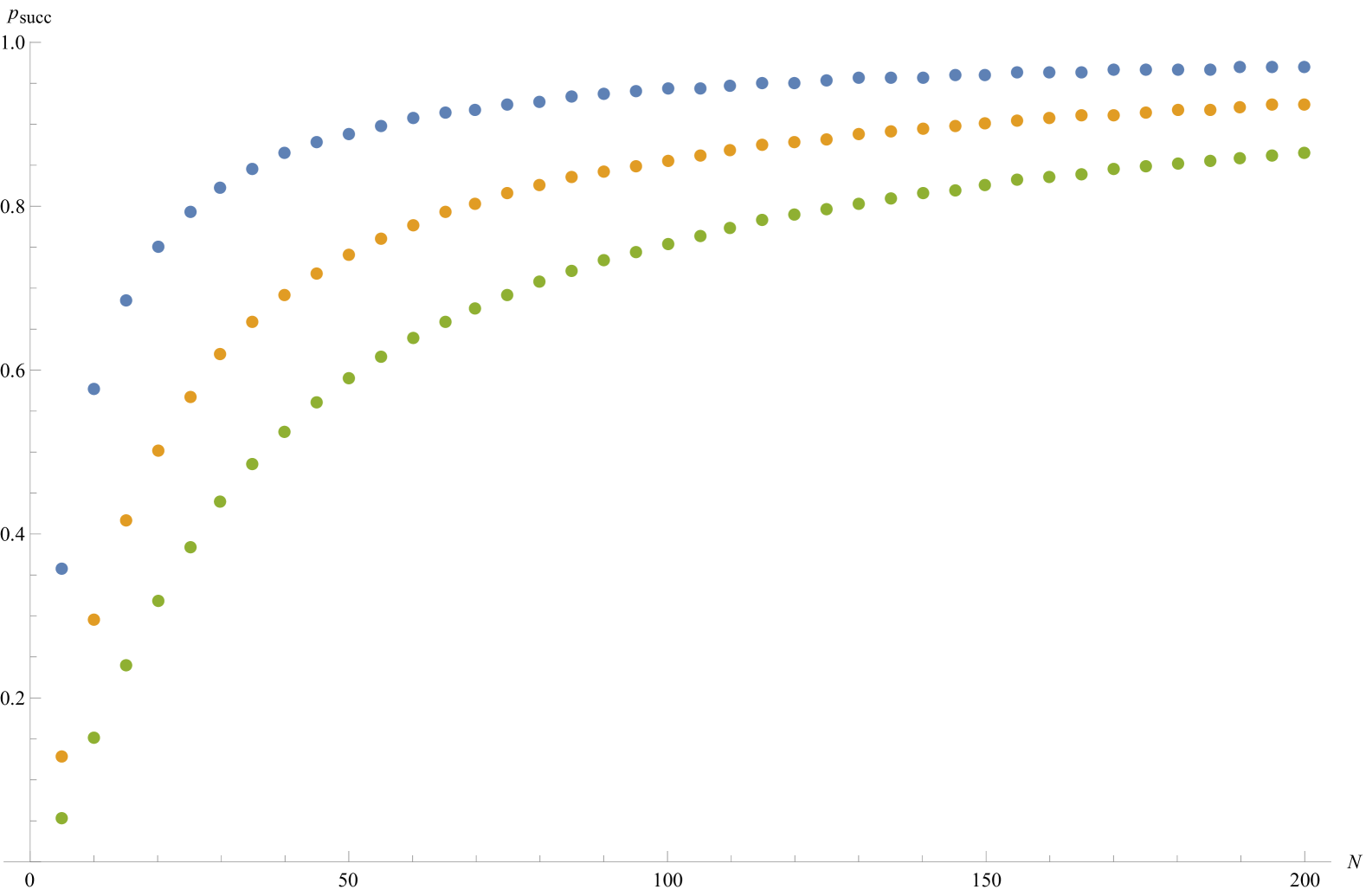
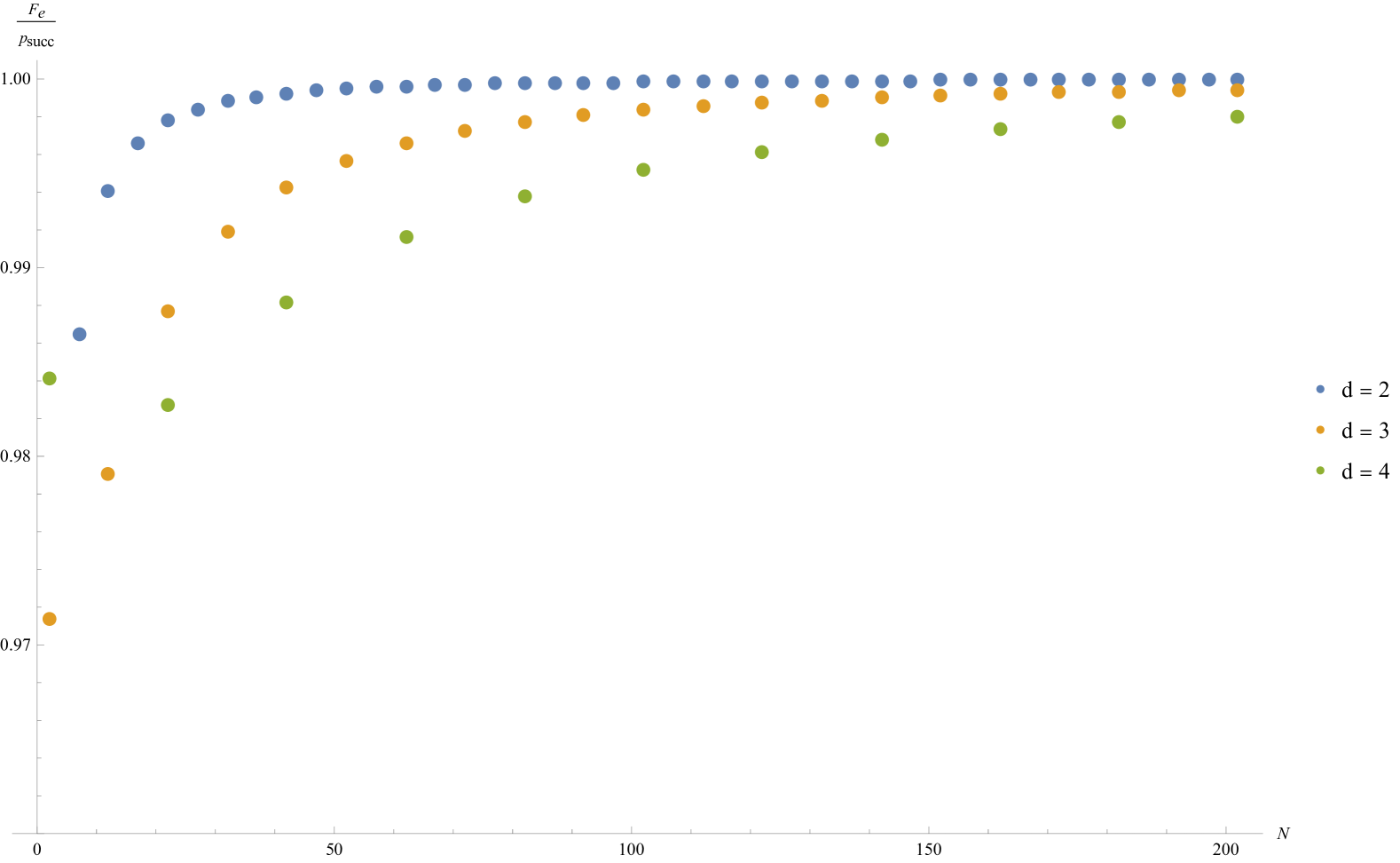
Figure 5. Numerical values of $p_{\mathrm{succ}}$ of two consecutive successful pPBT teleportations employing a recycled resource, as well as the conditional entanglement fidelity $F_{e}(\mathcal{N})/p_{\mathrm{succ}}$ of the corresponding teleportation channel $\mathcal{N}$ for $d\in\{2,3,4\}$

5.2. Probability of success

Recall, that for our two-step pPBT protocol we have:

$$\Pi_{0}^{\Lambda}=\begin{cases}I&\text{if $\Lambda=(\mu,\square)$},\\ 0&\text{if $\Lambda=(\lambda,\varnothing)$},\end{cases}\quad\quad\quad\sum_{k=1}^{N}\Pi_{k}^{\Lambda}=\begin{cases}0&\text{if $\Lambda=(\mu,\square)$},\\ I&\text{if $\Lambda=(\lambda,\varnothing)$},\end{cases}$$ (100)

and for the second round we have:

$$\widetilde{\Pi}_{0}^{\Lambda}=\begin{cases}I&\text{if $\Lambda=(\mu,\square)$},\\ 0&\text{if $\Lambda=(\lambda,\varnothing)$},\end{cases}\quad\quad\quad\sum_{k=1}^{N-1}\widetilde{\Pi}_{k}^{\Lambda}=\begin{cases}0&\text{if $\Lambda=(\mu,\square)$},\\ I&\text{if $\Lambda=(\lambda,\varnothing)$},\end{cases}$$ (101)

Computing $p_{\text{succ}}$ gives the following general formula, which depends on the amplitudes $f_{\lambda\cup a}$ of the resource state:

$$p_{\text{succ}}=\frac{1}{d^{2}}\sum_{\lambda\mathbin{\vdash}_{d}N-1}\left\lparen\sum_{a\in\mathrm{AC}_{d}(\lambda)}\frac{f_{\lambda\cup a}}{m_{\lambda\cup a}}\right\rparen\left\lparen\sum_{r\in\mathrm{RC}(\lambda)}m_{\lambda\setminus r}\right\rparen$$ (102)

In particular, for our two-step pPBT protocol this gives the following nice expression

$$p_{\text{succ}}=\frac{N(N-1)}{(N+d^{2}-1)(N+d^{2}-2)}$$ (103)

Notice that $p_{\text{succ}}$ coincides with probability of the success for the probabilistic multi-PBT.

6. Comparison with deterministic multi-PBT scheme

We can observe that the entanglement fidelity formula in eq.˜94 could also be used to get the performance of deterministic two-step recycling protocol. In particular, the matrix $M$ depends only on the choice of measurements in a two-step PBT scheme. Its highest eigenvalue gives the entanglement fidelity of the deterministic protocol, where the measurement effects $\Pi_{0}$ and $\widetilde{\Pi}_{0}$ are evenly distributed among the nonfailure effects $\Pi_{i}$ and $\widetilde{\Pi}_{i}$. The matrix $M$ can be viewed as an analogue of the teleportation matrix of the multi-dPBT teleportation from [MSK21]. Obtaining the exact formula for this eigenvalue as well as for the eigenvector seems beyond reach, so we provide numerical results in Fig.˜6 along with the performance of the corresponding multiport-based scheme.

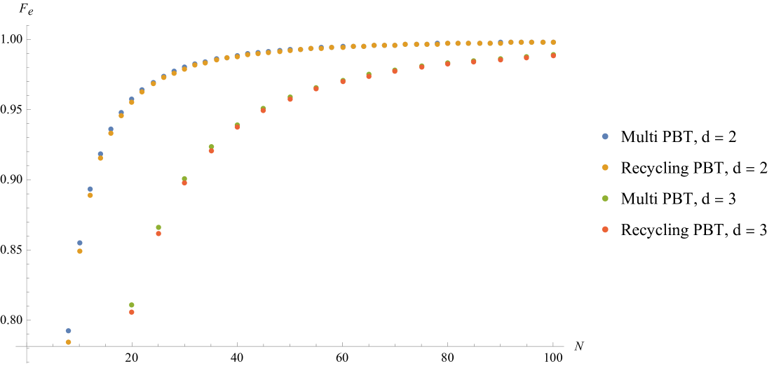
Figure 6. Comparison of deterministic two-step recycling PBT scheme with optimal deterministic multi PBT for two systems for $d\in\{2,3\}$.

7. Conclusions and open questions

Two main results are presented in this work. Firstly, the analysis of resource degradation is performed in the pPBT scheme. It is shown that in case of EPR resource, the degradation vanishes as the number of ports goes to infinity. This means that such a resource can be reused for further application of the pPBT protocol, meaning that it is an economical way to use a quantum resource, the preparation of which can be costly.

Moreover, a detailed analysis of the case of two subsequent successful applications of optimal pPBT protocols is compared to the teleportation of two quantum states at once, via a multiport-based scheme. This result shows that although such an approach provides smaller entanglement fidelity, the numerics show that for large $N$ the difference vanishes. Thus not only can two states be teleported with the repetitive use of a simpler measurement than a bigger joint measurement employed in the MPBT scheme, but it also means that two teleportations can be performed with a time delay.

The same reasoning is applied to the deterministic scheme. What is striking is that in this case, the two-step deterministic teleportation is close in terms of entanglement fidelity to the MPBT scheme even for small $N$, suggesting that the deterministic scheme is more suitable for recycling than the probabilistic one.

An open problem that arises from this work is developing an adapted measurement suited to the new distorted resource. This requires a reformulation of the problem in the form of a semidefinite program and is addressed by the ongoing research.

References

- [BCDFP10] Alessandro Bisio et al. “Optimal quantum learning of a unitary transformation” In Physical Review A 81.3 APS, 2010, pp. 032324 DOI: 10.1103/PhysRevA.81.032324
- [Ben+93] Charles H. Bennett et al. “Teleporting an unknown quantum state via dual classical and Einstein-Podolsky-Rosen channels” In Physical Review Letters 70.13, 1993, pp. 1895–1899 DOI: 10.1103/PhysRevLett.70.1895
- [BK11] Salman Beigi and Robert König “Simplified instantaneous non-local quantum computation with applications to position-based cryptography” In New Journal of Physics 13.9, 2011, pp. 093036 DOI: 10.1088/1367-2630/13/9/093036
- [Buh+16] Harry Buhrman et al. “Quantum communication complexity advantage implies violation of a Bell inequality” In Proceedings of the National Academy of Sciences 113.12, 2016, pp. 3191–3196 DOI: 10.1073/pnas.1507647113
- [Chr+20] Matthias Christandl et al. “Asymptotic Performance of Port-Based Teleportation” In Communications in Mathematical Physics, 2020 DOI: 10.1007/s00220-020-03884-0
- [DJR04] Thomas Decker, Dominik Janzing and Martin Rötteler “Implementation of group-covariant positive operator valued measures by orthogonal measurements” In Journal of Mathematical Physics 46.1 AIP Publishing, 2004 DOI: 10.1063/1.1827924
- [FTH23] Jiani Fei, Sydney Timmerman and Patrick Hayden “Efficient Quantum Algorithm for Port-based Teleportation”, 2023 arXiv: https://arxiv.org/abs/2310.01637
- [GBO23] Dmitry Grinko, Adam Burchardt and Maris Ozols “Gelfand-Tsetlin basis for partially transposed permutations, with applications to quantum information”, 2023 arXiv: https://arxiv.org/abs/2310.02252
- [GBO24] Dmitry Grinko, Adam Burchardt and Maris Ozols “Efficient quantum circuits for port-based teleportation”, 2024 arXiv: https://arxiv.org/abs/2312.03188
- [Gro+24] Frédéric Grosshans et al. “Multicopy quantum state teleportation with application to storage and retrieval of quantum programs”, 2024 arXiv: https://arxiv.org/abs/2409.10393
- [IH08] Satoshi Ishizaka and Tohya Hiroshima “Asymptotic Teleportation Scheme as a Universal Programmable Quantum Processor” In Physical Review Letters 101.24, 2008, pp. 240501 DOI: 10.1103/PhysRevLett.101.240501
- [IH09] Satoshi Ishizaka and Tohya Hiroshima “Quantum teleportation scheme by selecting one of multiple output ports” In Physical Review A 79.4, 2009, pp. 042306 DOI: 10.1103/PhysRevA.79.042306
- [Led22] Felix Leditzky “Optimality of the pretty good measurement for port-based teleportation” In Letters in Mathematical Physics 112.5, 2022, pp. 98 DOI: 10.1007/s11005-022-01592-5
- [May22] Alex May “Complexity and entanglement in non-local computation and holography” In Quantum 6 Verein zur Förderung des Open Access Publizierens in den Quantenwissenschaften, 2022, pp. 864
- [MHS14] Marek Mozrzymas, Michał Horodecki and Michał Studziński “Structure and properties of the algebra of partially transposed permutation operators” In Journal of Mathematical Physics 55.3, 2014, pp. 032202 DOI: 10.1063/1.4869027
- [MSH18] Marek Mozrzymas, Michał Studziński and Michał Horodecki “A simplified formalism of the algebra of partially transposed permutation operators with applications” In Journal of Physics A Mathematical General 51.12, 2018, pp. 125202 DOI: 10.1088/1751-8121/aaad15
- [MSK21] Marek Mozrzymas, Michał Studziński and Piotr Kopszak “Optimal Multi-port-based Teleportation Schemes” In Quantum 5 Verein zur Förderung des Open Access Publizierens in den Quantenwissenschaften, 2021, pp. 477 DOI: 10.22331/q-2021-06-17-477
- [MSSH18] Marek Mozrzymas, Michał Studziński, Sergii Strelchuk and Michał Horodecki “Optimal port-based teleportation” In New Journal of Physics 20.5, 2018, pp. 053006 DOI: 10.1088/1367-2630/aab8e7
- [NC97] M.. Nielsen and Isaac L. Chuang “Programmable Quantum Gate Arrays” In Phys. Rev. Lett. 79 American Physical Society, 1997, pp. 321–324 DOI: 10.1103/PhysRevLett.79.321
- [PBP21] Jason Pereira, Leonardo Banchi and Stefano Pirandola “Characterising port-based teleportation as universal simulator of qubit channels” In Journal of Physics A: Mathematical and Theoretical 54.20 IOP Publishing, 2021, pp. 205301
- [PLLP19] Stefano Pirandola, Riccardo Laurenza, Cosmo Lupo and Jason L Pereira “Fundamental limits to quantum channel discrimination” In npj Quantum Information 5.1 Nature Publishing Group UK London, 2019, pp. 50
- [QDSSM19] Marco Túlio Quintino et al. “Probabilistic exact universal quantum circuits for transforming unitary operations” In Phys. Rev. A 100.6 APS, 2019, pp. 062339 DOI: 10.1103/PhysRevA.100.062339
- [QDSSM19a] Marco Túlio Quintino et al. “Reversing Unknown Quantum Transformations: Universal Quantum Circuit for Inverting General Unitary Operations” In Phys. Rev. Lett. 123 American Physical Society, 2019, pp. 210502 DOI: 10.1103/PhysRevLett.123.210502
- [QE22] Marco Túlio Quintino and Daniel Ebler “Deterministic transformations between unitary operations: Exponential advantage with adaptive quantum circuits and the power of indefinite causality” In Quantum 6 Verein zur Förderung des Open Access Publizierens in den Quantenwissenschaften, 2022, pp. 679 DOI: 10.22331/q-2022-03-31-679
- [Qui21] Marco Túlio Quintino “Quantum teleportation beyond its standard form: Multi-Port-Based Teleportation” In Quantum Views 5 Verein zur Förderung des Open Access Publizierens in den Quantenwissenschaften, 2021, pp. 56
- [SBZ19] Michal Sedlák, Alessandro Bisio and Mário Ziman “Optimal Probabilistic Storage and Retrieval of Unitary Channels” In Phys. Rev. Lett. 122 American Physical Society, 2019, pp. 170502 DOI: 10.1103/PhysRevLett.122.170502
- [SHM13] Michał Studziński, Michał Horodecki and Marek Mozrzymas “Commutant structuture of Ux…xUxU* transformations” arXiv: 1305.6183 In J. Phys. A: Math. Theor. 46 (2013) 395303, 2013 URL: http://arxiv.org/abs/1305.6183
- [SHO13] Sergii Strelchuk, Michał Horodecki and Jonathan Oppenheim “Generalized Teleportation and Entanglement Recycling” In Physical Review Letters 110.1, 2013, pp. 010505 DOI: 10.1103/PhysRevLett.110.010505
- [SMK22] Michał Studziński, Marek Mozrzymas and Piotr Kopszak “Square-root measurements and degradation of the resource state in port-based teleportation scheme” In Journal of Physics A: Mathematical and Theoretical 55.37 IOP Publishing, 2022, pp. 375302 DOI: 10.1088/1751-8121/ac8530
- [SSMH17] Michał Studziński, Sergii Strelchuk, Marek Mozrzymas and Michał Horodecki “Port-based teleportation in arbitrary dimension” In Scientific Reports 7, 2017, pp. 10871 DOI: 10.1038/s41598-017-10051-4
- [Ste87] John R Stembridge “Rational tableaux and the tensor algebra of ” In Journal of Combinatorial Theory, Series A 46.1 Elsevier, 1987, pp. 79–120
- [WB16] Zhi-Wei Wang and Samuel L. Braunstein “Higher-dimensional performance of port-based teleportation” In Scientific Reports 6, 2016, pp. 33004 DOI: 10.1038/srep33004
- [WHS24] Adam Wills, Min-Hsiu Hsieh and Sergii Strelchuk “Efficient Algorithms for All Port-Based Teleportation Protocols” In PRX Quantum 5 American Physical Society, 2024, pp. 030354 DOI: 10.1103/PRXQuantum.5.030354
- [YKSQM24] Satoshi Yoshida et al. “One-to-one Correspondence between Deterministic Port-Based Teleportation and Unitary Estimation”, 2024 arXiv: https://arxiv.org/abs/2408.11902
- [YRC20] Yuxiang Yang, Renato Renner and Giulio Chiribella “Optimal Universal Programming of Unitary Gates” In Phys. Rev. Lett. 125 American Physical Society, 2020, pp. 210501 DOI: 10.1103/PhysRevLett.125.210501
- [YSM23] Satoshi Yoshida, Akihito Soeda and Mio Murao “Universal construction of decoders from encoding black boxes” In Quantum 7 Verein zur Förderung des Open Access Publizierens in den Quantenwissenschaften, 2023, pp. 957 DOI: 10.22331/q-2023-03-20-957